Pierre-Philippe Combes, Gilles Duranton, Laurent Gobillon ...

THE PRODUCTION FUNCTION FOR HOUSING: EVIDENCE FROM FRANCE

Pierre-Philippe Combes, Gilles Duranton, Laurent Gobillon

IEB Working Paper 2017/07

Cities


THE PRODUCTION FUNCTION FOR HOUSING:

EVIDENCE FROM FRANCE


The Barcelona Institute of Economics (IEB) is a research centre at the University of

Barcelona (UB) which specializes in the field of applied economics. The IEB is a

foundation funded by the following institutions: Applus, Abertis, Ajuntament de

Barcelona, Diputació de Barcelona, Gas Natural, La Caixa and Universitat de

Barcelona.

The Cities Research Program has as its primary goal the study of the role of cities as

engines of prosperity. The different lines of research currently being developed address

such critical questions as the determinants of city growth and the social relations

established in them, agglomeration economies as a key element for explaining the

productivity of cities and their expectations of growth, the functioning of local labour

markets and the design of public policies to give appropriate responses to the current

problems cities face. The Research Program has been made possible thanks to support

from the IEB Foundation and the UB Chair in Smart Cities (established in 2015 by

the University of Barcelona).

Postal Address:

Institut d’Economia de Barcelona

Facultat d’Economia i Empresa

Universitat de Barcelona

C/ John M. Keynes, 1-11

(08034) Barcelona, Spain

Tel.: + 34 93 403 46 46

[email protected]

http://www.ieb.ub.edu

The IEB working papers represent ongoing research that is circulated to encourage

discussion and has not undergone a peer review process. Any opinions expressed here

are those of the author(s) and not those of IEB.

mailto:[email protected]

http://www.ieb.ub.edu/


THE PRODUCTION FUNCTION FOR HOUSING:

EVIDENCE FROM FRANCE *


ABSTRACT: We propose a new nonparametric approach to estimate the production

function for housing. Our estimation treats output as a latent variable and relies on the

firstorder condition for profit maximisation with respect to nonland inputs by competitive

house builders. For parcels of a given size, we compute housing by summing across the

marginal products of nonland inputs. Differences in nonland inputs are caused by

differences in land prices that reflect differences in the demand for housing across

locations. We implement our methodology on newlybuilt singlefamily homes in France.

We find that the production function for housing is reasonably well, though not perfectly,

approximated by a CobbDouglas function and close to constant returns after correcting for

differences in user costs between land and nonland inputs and taking care of some

estimation concerns. We estimate an elasticity of housing production with respect to

nonland inputs of about 0.80..

JEL Codes: R14, R31, R32

Keywords: Housing, production function

* We thank seminar and conference participants and in particular David Albouy, Nate BaumSnow, Marcus Berliant,

Felipe Carozzi, Tom Davidoff, Uli Doraszelski, Gabe Ehrlich, JeanFrançois Houde, Stuart Rosenthal, Holger Sieg,

Matt Turner, Tony Yezer, and Oren Ziv for their comments and suggestions. We are also grateful to the Service de

l’Observation et des Statistiques (SOeS) Ministère de l’Écologie, du Développement durable et de l’Énergie for

giving us onsite access to the data and to Julian Gille and Benjamin Vignolles for their help with the data.

Pierre-Philippe Combes

Univ Lyon & CNRS & GATE-LSE UMR 5824

& Sciences Po & Centre for Economic Policy

Research

93 Chemin des Mouilles

69131 Ecully, France

E-mail: [email protected]

Gilles Duranton

Wharton School, University of Pennsylvania &

Center for Economic Policy Research, the

Spatial Economic Centre at the LSE, and the

Rimini Centre for Economic Analysis.

3620 Locust Walk

Philadelphia, PA 19104, USA


Laurent Gobillon

PSE-CNRS & Centre for Economic Policy

Research & Institute for the Study of Labor (IZA).

48 Boulevard Jourdan

75014 Paris, France





1. Introduction

We propose a new non-parametric approach to estimate the production function for housing.

Our estimation treats output as a latent variable and relies on the first-order condition for profit

maximisation with respect to non-land inputs by competitive house builders. For parcels of a

given size, we compute housing by summing across the marginal products of non-land inputs.

Differences in non-land inputs are caused by differences in land prices that reflect differences

in the demand for housing across locations. We implement our methodology on newly-built

single-family homes in France. We find that the production function for housing is reasonably well,

though not perfectly, approximated by a Cobb-Douglas function and close to constant returns after

correcting for differences in user costs between land and non-land inputs and taking care of some

estimation concerns. We estimate an elasticity of housing production with respect to non-land

inputs of about 0.80.

A good understanding of the supply of housing is important for a number of reasons. First,

housing is an unusually important good. It arguably provides an essential service to households

and represents more than 30% of their expenditure in both the us and France.1 It is also an

important asset. The value of the us residential stock owned by households was around 20 trillion

dollar in 2007 (Gyourko, 2009). French households owned about 4.6 trillion dollar worth of housing

in 2011 (Mauro, 2013). For both countries, this represents about 180% of their gross domestic

product.

Housing and the construction industry also matter to the broader economy. The construction

industry is arguably an important driver of the business cycle (e.g., Davis and Heathcote, 2005).

The role of housing in the great recession has been studied by, among others, Chatterjee and

Eyigungor (2015) and Kiyotaki, Michaelides, and Nikolov (2011). The broader effects of housing

are not limited to the business cycle. Housing has also been argued to affect a variety of aggre-

gate variables such as unemployment (Head and Lloyd-Ellis, 2012, Rupert and Wasmer, 2012) or

economic growth (Davis, Fisher, and Whited, 2014, Hsieh and Moretti, 2015).

Finally, and most importantly, housing is also central to our understanding of cities. Different

locations within a city offer different levels of employment and shopping accessibility and bun-

dles of amenities. Housing production is central in transforming the demand for locations from

households into patterns of land use and housing consumption. Unsurprisingly, housing is at the

heart of land use models in the spirit of Alonso (1964), Muth (1969), and Mills (1967) that form the

1See Combes, Duranton, and Gobillon (2016) for sources and further discussion of the evidence.

1

core of modern urban economics. Related to this, the welfare consequences of land use regulations

depend on the shape of the housing production function (Larson and Yezer, 2015). For instance,

the consequences of minimum lot size requirements will depend on how easily substitutable land

is in the production of housing.

Following Muth’s (1969, 1975) pioneering efforts, there is a long tradition of work that estimates

a production function for housing. Some of this work mirrors standard practice in productivity

studies and regresses a measure of housing output on land and other inputs. When we observe

the price of a transaction for a house, it is hard to separate between the price of housing per unit

and the quality-adjusted amount of housing that this house offers. Then, a regression of “housing”

on land and non-land inputs is likely to contain the unit price of housing in its error term. Since we

expect this price to determine non-land inputs, the regression will not appropriately identify the

production function for housing. This is a version of the unobserved price / unobserved quality

problem that usually plagues the estimation of production functions.2

A popular alternative is to estimate the elasticity of substitution between land and other inputs

directly by regressing the ratio of land to non-land inputs on the unit price of land. Because the

price of land is usually inferred from the value of a house minus the replacement cost of non-land

inputs, this regression suffers from reverse causation. With these caveats in mind, extant results

are generally supportive of constant returns to scale in the production of housing and estimates

for the elasticity of substitution between land and other inputs typically range between 0.50 and

0.75.3

To summarise, housing is highly heterogeneous and land, an immobile factor whose price is

often hard to observe, plays a particularly important role in its production. These features call for

specific estimation techniques, impose strong data constraints, and require careful attention to the

sources of variation used for identification.

To meet our first challenge and separate the quantity of housing from its price per unit, we

develop a novel estimation approach that relies on three main assumptions. First we assume a

production function for housing, which uses land and non-land inputs as primary factors.4 Since it

2See Ackerberg, Benkard, Berry, and Pakes (2007) and Syverson (2011) for discussion of the issues associated withthe estimation of production functions.

3Thorsnes (1997) is an interesting exception. He estimates an elasticity of substitution between land and other inputsstatistically undistinguishable from one using high-quality data for which he observes both the price of land prior toconstruction and the price of the house when it is sold.

4The notion of a production for housing services can be traced back to Muth (1960) and Olsen (1969).

2

cannot be directly observed, the quantity of housing is best thought of as a latent variable. Second,

house builders maximise profit. They choose how much non-land inputs to use in order to build

a house on a particular parcel of land given the price that households are willing to pay for each

unit of housing on this parcel. Third, we assume free entry among builders.

The first-order condition for profit maximisation by house builders implies that the marginal

value product of non-land inputs should be equal to their user cost. Then, under free entry, the

difference between the price of a house and the cost of the non-land inputs used to produce it

should be equal to the price of the land parcel. We can use this condition to eliminate the price

of housing from the first-order condition and obtain a partial differential equation where the

marginal product of non-land inputs depends on the quantity of housing produced and the cost

and quantity of both factors.5,6 Given parcel size, this partial differential equation can be solved

to obtain a non-parametric estimate of the amount of housing as a function of non-land inputs.

Because our estimation is conditional on parcel size, the production function for housing is only

partially identified.

The second challenge is to find appropriate data. Our methodology requires information about

the price of parcels, their size, and the cost of construction. The unique data we use satisfy these

requirements. They consist of several large annual cross-sections of land parcels sold in France

with a building permit for a single-family home and the cost of building this home.

Given our approach and the data at hand, the third challenge is to use an appropriate source

of variation. Although our estimation technique is non-standard, it remains that the supply of

housing can only be identified from variation in the demand for housing across parcels, not from

unobserved differences in supply conditions. We develop a procedure inspired by instrumental

variable approaches, which relies on systematic determinants of the demand for housing, namely

the urban area of a parcel and its location within this urban area. Housing located closer to the

5To estimate production functions, Gandhi, Navarro, and Rivers (2013) jointly use the first-order condition for profitmaximisation and the production function to eliminate unobserved persistent firm heterogeneity in productivity. Thisleads them to derive a partial differential equation similar to ours. For partial identification of the production functionof housing, we only rely on the integration of this differential equation. For full identification, we make further as-sumptions about returns to scale in production. By contrast, Gandhi et al. (2013) make assumptions about the dynamicsof productivity, insert the related equation into the production function and estimate the resulting specification thatincludes both the current and lagged values of inputs.

6Our approach consists in eliminating the unobserved price of output and rely about information on input pricesand quantities. An alternative solution to this problem is to impose further assumptions about the structure of demandas in Klette and Griliches (1996) or De Loecker (2011). The production function can then be recovered from an extendedproductivity regression. Because we do not observe revenue and industry structure and because standard assumptionsabout demand made for manufacturing goods are questionable in our context, this type of approach is not the mostappropriate here.

3

centre of Paris is more expensive than housing located further away in the suburbs. This is more

plausibly caused by differences in demand rather than by systematic differences in the ease of

construction, especially because we condition out many geographical characteristics that may be

correlated with supply factors.7

We obtain three main results. First, we find that the elasticity of housing production with respect

to non-land inputs is roughly constant at 0.80. As a first-order approximation, housing is produced

under constant returns to scale and is Cobb-Douglas in land and non-land inputs. This said, we

can nonetheless formally reject that the housing production function is Cobb-Douglas and constant

returns. We can also reject more general functional forms such as the ces. We find evidence of a

slight complementarity between land and capital and of small decreasing returns.

In the recent literature, we note the work of Yoshida (2016). He develops a new approach to

account for capital depreciation in housing and shows that standard estimates of the elasticity

of substitution between land and other inputs can be sensitive to how depreciation is accounted

for. Albouy and Ehrlich (2012) estimate a cost function for the production of housing at the city

level. Their objective is to explore the determinants and implications of differences in housing

productivity across cities. While our focus is to obtain a better measure of the amount of housing,

Albouy and Ehrlich (2012) measure it simply using standard hedonics in an intermediate step.

Our work is most closely related to Epple, Gordon, and Sieg (2010) and subsequent work by

Ahlfeldt and McMillen (2013) who also treat housing as a latent variable.8 We provide a detailed

comparison between our approach and Epple et al. (2010) below. For now, we note that, like us,

they develop a non-parametric estimation of the housing production function using restrictions

from theory. We nonetheless differ from their approach in several key respects. First, unlike us,

they assume constant returns to scale. For each unit of land, this assumption allows them to express

the first-order condition for profit maximisation with respect to capital in terms of the unit price

of housing. The latter is not observed but they show that it can be constructed as a monotonic

7When pointing at the similarity between our procedure and an instrumental variable approach, we mean thefollowing. We face a simultaneity problem where observed or unobserved confounding factors determine our variablesof interest, both the housing quantity to be estimated and the variables used to estimate it. This may obviously bias ourresults. We attempt to solve this problem by using the variation of appropriate surrogate variables instead of directlyusing the possibly contaminated variation of the variables used to estimate the housing quantity. This is consistent withthe spirit of extant instrumental variable approaches, even though we do not face the narrow issue of an endogenousexplanatory variable in a regression.

8In a different vein, Murphy (2015) structurally estimates a dynamic model of housing supply. He seeks to explainhow, where, and when housing is produced. His approach relies on a parametric first-order condition for profitmaximisation which allows him to recover the marginal cost of construction after having estimated its marginal benefit.The housing supply literature is surveyed in Gyourko (2009).

4

function of the value of housing per unit of land. Our approach shows that imposing constant

returns to scale is unwarranted. Second, they rely on different observables, namely housing values

per unit of land and land rent per unit instead of land rent and capital for each quantile of parcel

size. Third, we implement our approach on very different data: newly constructed houses for an

entire country instead of assessed land values for all houses for a single city, Pittsburgh. Finally,

we take steps towards disentangling demand and supply factors in land prices, an issue ignored

by Epple et al. (2010).9

2. Housing: treating output as a latent variable

House builders competitively produce housing services H using land T and non-land inputs K,

which we refer to as capital for convenience.10 House builders face a production technology

H(K,T) strictly increasing and concave in K. For now, land is exogenously partitioned into parcels

of area T where T is distributed over [T,T]. Section 7 considers the endogenous choice of parcel

size T by builders.

At a given location x, each unit of housing fetches a price P(x). This price reflects the willingness

to pay of residents to live at this location. In turn, the demand for locations is assumed to be driven

by factors such as employment and shopping accessibility or local amenities as in standard urban

models.11 For a parcel of size T located at x, the builder’s profit is π = P(x)H(K,T) − rK − R,

where r is the common user cost of capital and R is the endogenously determined (rental) price

of the parcel. Builders are competitive, take the price of housing and of parcels of size T at each

location as given, and are left to choose K.

9These differences notwithstanding, our results are broadly consistent with theirs and supportive of unitary elasticityof substitution between land and non-land inputs. When we implement their approach on our data, we find an elasticityof housing with respect to non-land inputs of 0.83.

10Non-land inputs are essentially labour and materials, which both get frozen into housing through the constructionprocess. This is consistent with the usual definition of capital.

11Monocentric urban models in the tradition of Alonso (1964), Muth (1969), and Mills (1967) define x as the distanceto the central business district (cbd) to which residents commute to work at a cost that increases with distance. Bothhousing services and a composite good enter utility. At the spatial equilibrium, residents at each location choose howmuch housing and composite good to consume given the local price of housing. Prior to this, they chose their locationoptimally to maximise utility. At the spatial equilibrium, utility is equalised across locations. The model is often solvedusing the ‘bid-rent approach’ by deriving the maximum price that residents are willing to pay subject to achievinga given level of (equilibrium) utility (Fujita, 1989, Duranton and Puga, 2015). Then, given the price of housing at alocation, competitive builders choose how much housing to build at this location. Our approach is fully consistent withthis standard modelling of land use and urban development but it is more general because we do not need to imposeany specific geography. We only use the geography of cities as part of our identification strategy below.

5

The first-order condition for profit maximisation with respect to capital is,

P(x)∂H(K,T)

∂K= r . (1)

The optimal amount of capital inputs that satisfies this condition is given implicitly by K∗ =

K∗(P(x),T). Because the production function for housing H(.,.) is concave in K, K∗ is unique given

T. Applying the implicit function theorem to the profit maximisation programme, the concavity of

H(.,.) also implies that ∂K∗/∂P > 0. Hence, there is a bijection between the price of housing and

the profit-maximising level of capital for any T and we can write P(x) = P(K∗,T).

Free entry implies that the profits from building are dissipated into the price of land so that,

R = P(K∗,T)H(K∗,T)− rK∗ ≡ R(K∗,T) . (2)

Note that the price of land in equilibrium is uniquely defined for any K∗ and T.

We can insert equation (1) into (2) to eliminate the unit price of housing, which is not observed

in the data, to obtain the following partial differential equation:

∂H(K∗,T)∂K∗

=r H(K∗,T)

rK∗ + R(K∗,T). (3)

For consistency with our empirical work below, this expression may be more intuitively rewritten

by transforming its left-hand side into an elasticity:

∂ log H(K∗,T)∂ log K∗

=rK∗

rK∗ + R(K∗,T), (4)

where log denotes a natural logarithm. In words, the elasticity of housing with respect to (profit-

maximising) capital is equal to the share of capital in the cost of building a house.

Consider that for a given parcel of size T, the desirability of locations varies so that the price

of housing is distributed over the interval[P,P]. The optimal level of capital in housing K∗ then

covers the interval[K,K

]where K = K∗(P,T) and K = K∗(P,T). The solution to the differential

equation (4) for a given value of the optimal amount of capital inputs K∗ in this interval is obtained

by integration and can be written as:

log H(K∗,T) =∫ K∗

K

rKrK + R(K,T)

d log K + log Z (T) . (5)

where Z(T) is a positive function equal to H(K,T). Equation (5) enables the computation of the

number of units of housing on parcels of size T knowing the prices of those parcels and the

amounts of capital invested to build on these parcels.

6

The intuition behind this result is relatively straightforward. Locations differ in desirability and

thus in their unit price for housing. This price is not observed but it appears in both the optimal

capital investment rule described by the first-order condition (1) and in the zero-profit condition

(2). We can use the latter equation to substitute for the price of housing in the former and derive

differential equation (3), or its log equivalent (4). We then readily obtain log H by integration over

log K in equation (5).

To illustrate the workings of equation (5) and check the consistency of our approach, consider

first a Cobb-Douglas production function. In this case, the price of land R and the cost of capital

used to build a house r K are proportional. This implies that the term within the integral is

constant.12 As a result, log H is proportional to log K. That is, we retrieve a Cobb-Douglas form.

To take another example, assume now that the production function enjoys a constant elasticity

of substitution between land and capital equal to two. In this case, profit maximisation implies

that capital inputs should increase with the square of the price of parcel of size T. Integrating

the share of capital as in equation (5) implies that the production of housing is proportional to

(√

K + b)2 where b is a constant. This functional form is indeed the generic functional form for a

ces production function with an elasticity of substitution equal to two when a factor (land) is held

constant.

An important assumption of our model is that the price of land for a parcel is affected by its

location x only through the price that residents are willing to pay to live at this location. That

is, the price of land is determined entirely by the demand side. Put differently, our approach so

far does not allow for a parcel characteristic y to affect the production technology directly. To

understand the implications of supply differences across parcels, let us consider first a simple

example where all parcels are of unit size, the demand for housing is the same at all locations,

P(x) = P = 1, and the price of capital inputs is normalised to unity, r = 1. Assume that housing

is produced according to H(K,y) = 1a Ka y1−a where the unobserved characteristic y measures the

ease of construction. Then, in equilibrium, capital is given by K(y) = y and parcel prices capitalise

the ease of construction, R(y) = 1−aa y = 1−a

a K. Using equation (5) to estimate the value of housing,

we would obtain that the production of housing is proportional to K instead of being proportional

to Ka.13

12This property was already noted by Klein (1953) and Solow (1957).13Note that this problem of missing variable is worse than in standard cases because it creates a bias even when the

missing characteristic y is uncorrelated with P as illustrated by our example.

7

More generally, assume that parcels are now characterised by two location characteristics, x

and y. The characteristic x still affects the price that residents are willing to pay, P(x), while y

affects the production of housing directly, which is now given by H(K,T,y). The analogue to the

first-order condition (1) is P(x)∂H(K,T,y)/∂K = r. The zero-profit condition also implies that

y affects the price of land directly: R(K∗,T,y) = P(x)H(K∗,T,y) − rK∗. The partial differential

equation analogous to (4) is:

∂ log H(K∗,T,y)∂ log K∗

=rK∗

rK∗ + R(K∗,T,y). (6)

It can be solved only for a given y. Integrating as we do in equation (5) ignoring y will be

problematic since y will be correlated with both the quantity of housing H and the price of land

R. Locations with a particularly good y will both be able to generate more housing for a given

amount of capital and face a higher price for land. Below, we develop a procedure inspired by

instrumental variable approaches to circumvent this problem.

Some of our other assumptions must be discussed further. First, we assume non-increasing

marginal returns to capital. This is arguably an appropriate assumption for newly constructed

single-family homes. Second, because of the ease of entry in this industry and the absence of fine

product differentiation, our assumption of competitive builders also strikes us as reasonable.14

Third, at every location, the unit price of housing is taken as given by competitive builders. We

thus implicitly assume an integrated housing market and (fairly) homogenous preferences. This

is defensible in our empirical application below since we ignore outliers and in robustness checks,

we consider the construction cost of houses at early stages of completion and conduct separate

estimations for different socio-economic groups of buyers. Finally, parcels are exogenously deter-

mined. Treating land as a fixed input is reasonable in France where zoning rules usually prevent

the subdivision of existing parcels in residential areas. We discuss further identification issues

below with our empirical strategy.

We can now compare our approach to that of Epple et al. (2010). Appendix A provides formal

derivations. The first difference is that our approach relies on using capital K, parcel prices R,

and land areas T, whereas Epple et al. (2010) use house values P H instead of capital together

14A search on the French yellow pages (http://www.pagesjaunes.fr/) yields 1783 single-family house builders forParis (largest urban area with population above 12 million), 111 for Rennes (10th largest urban area with population654,000), and still 38 for Troyes (50th largest urban area with population 188,000). (Search conducted on 21st May 2013

looking for ‘constructeurs de maisons individuelles’ – builders of single family homes – typing ‘Ile-de-France’ to capturethe urban area of Paris, ‘Rennes et son agglomération’, and ‘Troyes et son agglomération’ for the other two cities.)

8

http://www.pagesjaunes.fr/

with parcel prices and land areas. This difference is nonetheless mostly cosmetic because both

our approach and that of Epple et al. (2010) rely on the same zero-profit condition P H = r K + R.

Hence, land values can be immediately recovered from capital investments and parcel prices just

like capital can be recovered from house values and parcel prices. The second difference is that

we do not impose constant returns to scale in the production of housing. This difference is again

superficial. We show that the approach of Epple et al. (2010) can readily be modified to lead to the

same partial identification results when dispensing with constant returns.

The main substantive difference is that our approach is more direct and uses the first-order

condition for profit maximisation after eliminating the unobserved unit price of housing. The

approach of Epple et al. (2010) relies instead on duality theory and Hotelling’s lemma to recover

the supply function of housing before its production function. This is a less direct route that relies

on a more intricate differential equation for which there is no closed-form solution. As explained

above, we also expand our approach to account for the possible simultaneity between capital and

parcel prices.

3. Estimation of the housing production function

There are four main steps to our empirical approach. We first predict the price of parcels R for

pairs of capital K and parcel size T on a grid using kernel smoothing. Next, we estimate non-

parametrically the amount of housing H(K,T) for a given T using equation (5) and quantities

computed at values of K on the grid. We then describe the shape of H(K,T) by means of simple

regressions. The same approach is implemented with and without conditioning out supply factors

that may affect R, K, and T prior to smoothing.

3.1 Empirical strategy

We use equation (5) to compute housing by integrating a cost share over values of K for a given T.

In the data, the price of parcels of a given size is observed only for some values of capital, not for

the entire continuum. As a consequence, for a given level of capital K and parcel size T on the grid,

we estimate the price of land from slightly larger and slightly lower values of K and/or T using a

kernel non-parametric regression. The price of land and capital at points on the grid are then used

to compute the integral that defines the production function of housing.

9

The kernel we use in non-parametric regressions is the product of two independent normals and

the bandwidth is computed using a standard rule of thumb for the bivariate case (see Silverman,

1986).15 For a given value of (K,T) on the grid, the estimated price of land is given by the following

formula:

R (K,T) = ∑i

ωiR (Ki,Ti) with ωi =LhK (K− Ki) LhT (T − Ti)

∑i LhK (K− Ki) LhT (T − Ti), (7)

where N is the number of observations, Lh (x) = 1h f( x

h

)with f (·) the density of the normal

distribution, and hX = N−1/6σ (X) with σ (X) the empirical standard deviation for variable X

computed from the data. This kernel estimator has the property of making R(K,T) unique, which

is requested by our model.16

The lower bound of the integral entering equation (5) is the lowest value of the profit-

maximising capital. In practice, we can potentially use any value of capital as lower bound, K,

but there is a trade-off. A small value for the lower bound will allow us to study the variations

of the housing production function over a wide range of values for capital inputs but this may

come at the cost of being in a region where there are few observations. In our work below, we

restrict attention to observations above the first decile (and below the ninth decile) to estimate the

production of housing.

The integral entering (5) is computed using a trapezoidal approximation such that an estimator

of the production function at a given grid node(Kg

i ,T)

is:

log H(Kgi ,T) =

i

∑j=2

(cj−1 + cj

2

)(log Kg

j − log Kgj−1

), (8)

where Kgj , j = 1,...,J are the grid values of capital and:

cj =rKg

j

rKgj + R(Kg

j ,T). (9)

After smoothing the data and estimating the production of housing, we regress the non-

parametrically estimated housing production on capital inputs. We estimate these regressions

to describe how housing production varies with capital. For instance, under Cobb-Douglas, for

any fixed T, there should be a linear relationship between the log of the amount of housing

15Alternatively, we could consider that the integrand rKrK+R(K,T) is computable only at the observed values of capital

and recover that integrand for other value of capital using a kernel non-parametric regression of the integrand.16Even if the whole sample of land transactions is involved in the estimation, only transactions with values of (K,T)

‘close enough’ to points on the grid significantly contribute to the estimation of land prices since we use a kernel thatputs more weight on these transactions in the computations.

10

produced and log capital. In section 6, we further assess a variety of alternative functional forms by

comparing our non-parametric estimates of housing production to estimates for which we impose

a functional form in the first place (instead of kernel-smoothing the data).17

3.2 Dealing with supply-side unobserved heterogeneity

As already mentioned, our approach relies on the fact that the price of a parcel should only

reflect the price that housing can fetch on this parcel. However, the price of a parcel may also

reflect the ease of construction. For instance, a parcel may be more costly to develop because of a

steep slope or because it is harder to excavate. For a given price of housing at this location, this

parcel will be worth less in equilibrium. More generally, consider a location characteristic y that

affects the optimal investment in capital and thus the price of a parcel. By equation (6), we can

only appropriately estimate the production function for housing for a given y (which may not be

observed).

To deal with that problem, our empirical strategy is to purge our variables of interest, R and

K, from the effects of supply characteristics by relying only on the variations in the demand for

housing across locations. In practice consider the following regression:

log Ri = Xi aR + Yi bR + f R(Ti) + εRi , (10)

where X is a vector of location characteristics that (are assumed to) affect the demand for housing,

Y is a vector of location characteristics that (are assumed to) affect the supply of housing, εRi

is an error term, and f R(T) is a potentially non-parametric function of T. The vector X is the

empirical counterpart of the location effect x in our framework above while Y is the empirical

counterpart to y. To estimate f R(T), we use indicator variables for every size centile. Then, under

the assumption that the residual follows a normal law, we can compute an unbiased predicted

land price Ri which depends only on demand characteristics and not on supply characteristics:

Ri = exp(Xi aR + Y bR + f R(Ti) + (σR)2/2) where Y bR is the mean effect of supply characteristics

and σR is the estimator of the standard deviation of the error term of the regression described by

equation (10).

The location characteristics Y that affect the price of parcels through the supply of housing will

also affect the optimal use of capital and, in turn, bias our estimates. Hence, we also want to

17We prefer this approach to more standard specification tests that tradeoff a measure of goodness of fit against thenumber of explanatory variables using arbitrary weights.

11

estimate the following regression analogous to equation (10) for capital:

log Ki = Xi aK + Yi bK + f K(Ti) + εKi . (11)

Like with parcel prices, we can then compute a predicted value for capital K which depends

only on demand characteristics: Ki = exp(Xi aK + Y bK + f K(Ti) + (σK)2/2) where Y bK is the

mean effect of supply characteristics and σK is the estimator of the standard deviation of the

error term in equation (11). We can then use predicted instead of actual capital when estimating

non-parametrically prices of land from equation (7).

As sources of exogenous demand variation, we use the urban area to which a parcel belongs

and the distance to its centre. This is consistent with monocentric urban models in the tradition of

Alonso (1964), Muth (1969), and Mills (1967) where the price of housing, land prices, and capital

investment at each location are fully explained by the distance to the centre and city population.

We also use local measures of income which also play a role in more elaborate models of urban

structure with heterogeneous residents (Duranton and Puga, 2015).

This said, we worry that the urban area of a parcel or its distance to the centre may be corre-

lated with the ease of building. For instance, construction labour may be cheaper in some cities

(Gyourko and Saiz, 2006) or terrains characteristics may vary systematically with distance to the

centre. This is why we also include a number of geographic municipal characteristics as part of

our vector of supply characteristics Y to be conditioned out. In addition, we can condition out the

local wage of blue-collar workers in the construction industry from urban area fixed effects since

construction costs may vary across cities.18

More specifically, to estimate equations (10) and (11), we include urban area fixed effects,

distance to the centre (allowing the effect to vary across urban areas), three municipal socioeco-

nomic characteristics (log mean income, its standard deviation, and the share of population with

university degree), and seven geological variables (ruggedness, and three classes of soil erodability,

soil hydrogeological class, and soil dominant parent material). In our demand vector, we include

urban area fixed effects (after conditioning out local wages for construction workers), distance to

the centre, and municipal socioeconomic characteristics. We verify that our results are robust to

18Wages in the construction industry in an urban area cannot be directly included in the regression because theywould be collinear with urban area fixed effects but we can regress urban area fixed effects on wages in the constructionindustry and retain the estimated residual.

12

using more restrictive or more inclusive definitions of the demand determinants.19

Finally, recall that our model takes parcel size T as given. The location characteristics that affect

the cost of construction may also affect parcel size. For instance, parcels may be larger where

construction is more costly. This suggests applying the same approach as in equation (10) to parcel

size and estimate:

log Ti = Xi aT + Yi bT + εTi . (12)

The resulting predicted values Ti = exp(Xi aT + Y bT + (σT)2/2)) can then be used instead of the

actual parcel sizes to estimate parcel values non-parametrically in equation (7). When we also

allow for T to depend on a supply factor, we need to amend equations (10) and (11) above and

consider instead the following two equations

log Ri = Xi aR + Yi bR + εRi , (13)

log Ki = Xi aK + Yi bK + εKi . (14)

where we no longer include T as determinant of R and K.

Our identification strategy relies on the same kind of principles as standard instrumental

variables approaches because it uses the (conditional) variation of surrogate variables, such as

the urban area of a parcel in our case, rather than the entire variation of the variable of interest.

While the principle is the same, our implementation differs considerably from standard two-stage

least-squares procedures. Our objective is to provide a non-parametric estimate of housing, H, as

a function of capital, K, for a given parcel size, T. Given that observed and unobserved supply

characteristics of parcels are expected to affect capital, land values, and parcel size, our ‘first stage’

generates predicted values for three variables, capital K, land values R, and parcel size T. We then

estimate housing production as when we use gross values of K, R and T.20

To address more directly the issue of differences in labour costs and other possible forms

of supply heterogeneity across cities, we would like to estimate a separate housing production

function for each urban area separately. Except for the largest French cities, the number of parcel

19We retain the same rich specification throughout but vary the composition of X. We also experimented withspecifications with fewer control variables and obtained similar results. We do not report these results here.

20Although we may use as little as one demand-related characteristic (such as the location relative to the centre) topredict three variables in the first step, the effect of capital on housing production is nonetheless identified with ourprocedure. We are not in a situation where we attempt to estimate the effect of three endogenous explanatory variableswith one instrumental variable. Instead, we use surrogate variables to predict a triplet (K,R,T) (or only the pair (K,R)).In effect, we use predicted values of K and R to estimate log H (given actual or predicted T).

13

transactions in a typical urban area is unfortunately too small to do this. We nonetheless divide

urban areas into size classes and perform a separate estimation for each size class.

Measurement error on capital inputs K or land prices R may also affect our estimation. Mea-

surement error is dealt with in two different ways in our approach. First, as mentioned above, we

kernel-smooth parcel price data. Second, our approach based on predicted values for R, K, and T

is less prone to measurement error than the use of observed values.

As already highlighted, our model assumes an integrated market for housing. This is what

allows us to think in terms of units of housing that can be measured and compared across houses.

A full relaxation of the integrated market assumption would involve considering each house as

a uniquely differentiated variety over which residents have idiosyncratic preferences. When all

residents value all houses differently, the notion of a common unit of housing is no longer well

defined. While our approach is unable to deal with such extreme cases, in a robustness check, we

consider housing markets segmented across socio-economic groups using information about the

characteristics of the buyers.

To address product differentiation in housing, we can also use the fact that the reported con-

struction costs are for one of three levels of completion (‘fully finished’, ‘ready to decorate’, and

‘structure completed’). Should idiosyncratic preferences affect building costs, we expect they will

matter more for houses at a more advanced state of completion. We can thus assess the importance

of demand heterogeneity indirectly by comparing results across the different stages of completion.

We need to keep in mind that housing construction is tightly regulated in France as in many

other countries. The three main regulatory instruments are (i) the zoning designation, (ii) the

maximum intensity of development, and (iii) severe restrictions on parcel division.21 The zon-

ing designation indicates whether a parcel can be developed and, if yes, whether this can be

for residential purpose. Given that we only observe parcels with a development permit for a

single-family home, this creates no further issue beyond the fact that we estimate the production

function for single-family homes in parcels designated for that purpose. Turning to the maximum

intensity of development that applies to a parcel, this information is not centrally collected by the

French government. Although we emphasise that the quantity of housing is not solely determined

21The maximum intensity of development is essentially a maximum floor-to-area ratio (far) regulation. In France, itis referred to as the ‘coefficient d’occupation des sols’ (cos). This regulation is subject to national guidelines but can beadjusted locally by the municipality. Other regulations such as minimum parcel size or an obligation to follow a localstyle with more or less stringency also often apply.

14

by the square-footage of a house, we nonetheless acknowledge that we estimate the production

function for housing under prevailing restrictions on residential development. Absent regulations,

single family homes would perhaps be different from what they are under the current regulatory

regime.22 However, we are interested in estimating how land and capital inputs are transformed

into housing under the current regulatory constraints. While knowing how regulations affect the

production of housing is certainly a question of interest, this is not one that we can answer here.

Finally, we acknowledge further limitations of our framework. First, as already noted, the price

of housing on a parcel is only determined by its location, not by the intensity of development on

this parcel.23 The second issue is that single-family homes are indivisible (by definition) and the

price per unit of housing may decline with the quantity of housing offered by a house, at least

beyond a certain quantity. Second, our model is static and ignores that housing development is,

to a large extent, an irreversible decision. In turn, this implies that the price of vacant land may

include the option value to develop it.24 Note also that we estimate the production function for

one house not for builders who may build several houses. In particular, there might be sizeable

economies of scale arising from being able to build many houses at the same location at the same

time.

3.3 Implementation

To implement our approach, for each of the nine deciles of parcel size, we consider 900 values

of capital uniformly distributed over the interval defined by the first and last deciles of capital

within the parcel size decile at hand. This generates a fine grid of 8,100 (K,T) points. We first

estimate parcel prices at any point of the grid using equation (7) with up to 386,181 observations

for the entire country in our data set. Then, for each of the nine deciles of parcel size, the housing

production function is estimated using equation (5) by summing over the values of capital within

the parcel size decile at hand, using trapezoids to approximate the integral. By construction, for

any parcel size decile, the lower bound of integration K corresponds to the bottom decile and the

maximum upper bound K to the top decile of capital values. This avoids having our estimations

influenced by potential outliers or by observations that belong to a different market segment such

22To be concrete, consider that two technologies with very different production functions are available to buildhousing. If one technology is banned through regulations, we can only learn about the second.

23Demand for housing on a parcel might decline with the intensity of development on this parcel. This is certainly anissue for multi-family buildings. It should be less problematic with single-family homes.

24See Capozza and Helsley (1990) and subsequent literature or Duranton and Puga (2015) for a review.

15

as luxury homes. We obtain 8,100 values of housing production, corresponding to 900 values of

capital for each of the nine parcel size deciles.

Before turning to our results, several implementation issues must be discussed. Our model

relies on the rental value of land and the rental value of capital inputs. The data we use only report

the price of land and the cost of construction. Using stocks (transaction values) instead of flows

(rental values) makes no difference to our approach when the user cost of land is the same as the

user cost of capital. This is not the case when the user costs differ across factors.25 Following

Combes et al. (2016), we take the annual user cost of capital to be 6%. This reflects a long term

interest rate of 5% and a 1% annual depreciation.26 For the user cost of land, we take a value of 3%

per year.27 To make parcel prices and capital investments comparable over time, we also correct

for year effects which we obtain from regressions of log parcel prices and log capital on year fixed

effects.

Finally, confidence intervals are estimated by bootstrap. At each iteration, a random sample is

drawn with replacement from the universe of all transacted land parcels. Parcel prices are recom-

puted at each point of our (K,T) grid using kernel non-parametric regressions before re-estimating

housing production. The distribution of values for housing production at each point of the grid is

then recovered and confidence intervals can be deduced.

4. Data

The observations in our data are transacted land parcels with a building permit that are extracted

from the French Survey of Developable Land Price (Enquête prix des terrains à bâtir, EPTB). This

survey is conducted every year in France since 2006 by the French Ministry of Ecology, Sustainable

Development, and Energy. The sampling frame is drawn from Sitadel, the official land registry,

which covers the universe of all building permits for detached houses. The survey selects building

permits for owner-occupied, single-family homes. Permits for extensions to existing houses are

25This is very much in the spirit of the user-cost correction first proposed by Poterba (1984).26In the French national accounts, housing depreciation can be computed as the difference between investment in

housing and the increase in housing stocks. According to Commissariat Général au Développement Durable (2012),this difference in 2009 was about 15 bn Euros, which corresponds to slightly less than 1% of gdp or just below 0.6% ofthe value of the stock. This is arguably a lower bound as much housing maintenance falls under home production andis not accounted for in national accounts.

27As estimated by Combes et al. (2016), the elasticity of land prices with respect to local income is slightly above onewhile the elasticity of the price of land with respect to population is slightly below one. A 1% annual increase in incomeand a 1% annual increase in population (the mean urban population growth in France in the recent past) thus imply anabout 2% annual appreciation of land prices to be deducted from the long run interest rate of 5%.

16

excluded. A small fraction of parcels (less than 3% in 2006) also has a demolition permit. Our

study period is from 2006 to 2012.28 Originally, about two thirds of the transactions with permits

were sampled. The survey became exhaustive in 2010. This survey is mandatory and the response

rate, after one follow-up, is above 75%. Annually, the number of observations ranges from 48,991

in 2009 to 127,479 in 2012.

While it is possible to get new houses built in many ways in France, the arrangement we study

covers a large fraction of new constructions for single-family homes.29 Households typically first

buy constructible land, obtain a building permit, and get a house built by themselves, through

a general contractor, or an architect. Only about 20% of new houses are ‘self-built’ as French

law requires the use of a general contractor or an architect for constructions above 100,000 Euros.

Getting a new house by first buying land subsequently signing a contract with a builder is fiscally

advantageous as it avoids paying stamp duties on the structure.30 This arrangement also greatly

reduces financing constraints for house builders and lowers their risks.

For each transaction, we know the price of the parcel, its size, whether it is ‘serviced’ (i.e.,

has access to water, sewerage, and electricity), its municipality, how it was acquired (purchase,

donation, inheritance, other), some information about its buyer, whether the parcel was acquired

through an intermediary (a broker, a builder, another type of intermediary, or none), and some

information about the house built, including its cost (but with no breakdown between material

and labour). The notion of building costs may be ambiguous but we know whether the reported

cost reflects the cost of a fully decorated house, the cost of a serviced house prior to decoration

(i.e., excluding interior paints, light fixtures, faucets, kitchen cabinets, etc), or only the cost of the

bare-bone structure. Ready-to-decorate houses represent the large majority of our observations

(72%). We only retain parcels that were purchased and ignore inheritances and donations. We also

appended a range of municipal and urban area characteristics described in Appendix B.

Table 1 provides descriptive statistics for all our main variables. The first interesting fact is the

considerable variation in parcel size, total construction costs, and parcel price per square meter. A

28It is important to keep in mind that, unlike in the us, there was no housing burst in France during this period andthat the heterogeneity of housing price fluctuations across cities was far from being as extreme as in the us.

29The consultancy Développement-Construction reports between 120,000 and 160,000 new single-family homes peryear during the period (http://www.developpement-construction.com/). These magnitudes closely coincide with thenumber of observations in later years after accounting for the response rate.

30This tax avoidance is only partially offset by a vat abetment for construction costs. Stamp duties in France currentlyrepresent about 5.8% of the value of the transaction exclusive of notary and various ancillary fees.

17

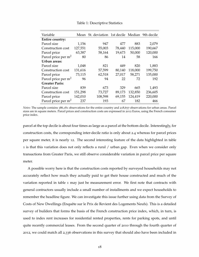
http://www.developpement-construction.com/

Table 1: Descriptive Statistics

Variable Mean St. deviation 1st decile Median 9th decileEntire country:Parcel size 1,156 947 477 883 2,079Construction cost 127,551 55,003 78,440 115,000 190,667Parcel price 63,387 58,164 19,673 50,000 120,000Parcel price per m2 80 86 14 58 166Urban areas:Parcel size 1,048 821 449 820 1,883Construction cost 131,616 57,599 80,140 118,000 199,750Parcel price 73,115 62,518 27,017 58,271 135,000Parcel price per m2 96 94 22 72 192Greater Paris:Parcel size 839 673 329 665 1,493Construction cost 151,298 73,727 89,173 132,850 236,605Parcel price 142,010 108,598 69,155 124,419 220,000Parcel price per m2 237 193 67 182 466

Notes: The sample contains 386,181 observations for the entire country and 218,657 observations for urban areas. Parcelsizes are in square meters. Parcel prices and construction costs are expressed in 2012 Euros, using the French consumerprice index.

parcel at the top decile is about four times as large as a parcel at the bottom decile. Interestingly, for

construction costs, the corresponding inter-decile ratio is only about 2.4 whereas for parcel prices

per square meter, it is nearly 12. The second interesting feature of the data highlighted in table

1 is that this variation does not only reflects a rural / urban gap. Even when we consider only

transactions from Greater Paris, we still observe considerable variation in parcel price per square

meter.

A possible worry here is that the construction costs reported by surveyed households may not

accurately reflect how much they actually paid to get their house constructed and much of the

variation reported in table 1 may just be measurement error. We first note that contracts with

general contractors usually include a small number of installments and we expect households to

remember the headline figure. We can investigate this issue further using data from the Survey of

Costs of New Dwellings (Enquête sur le Prix de Revient des Logements Neufs). This is a detailed

survey of builders that forms the basis of the French construction price index, which, in turn, is

used to index rent increases for residential rented properties, rents for parking spots, and until

quite recently commercial leases. From the second quarter of 2010 through the fourth quarter of

2012, we could match all 2,336 observations in this survey that should also have been included in

18

Figure 1: Probability distribution function of the relative distance for new constructions, Frenchurban areas 2006-2012

0

0.2

0.4

0.6

0.8

1

1.2

1.4

1.6

1.8

0 0.1 0.2 0.3 0.4 0.5 0.6 0.7 0.8 0.9 1

Relative distance

Density

Notes: All years of data used. 218,657 observations. For each new construction, we compute the distance between thecentroid of its municipality and the centroid of its urban area and divide by the greatest observed distance for any newconstruction in this urban area.

our main data using the building permit identifier. Reassuringly, the correlation between the two

measures of housing costs is 0.83 both in levels and in logs.

Rather than reflecting mis-measurement, the variation in prices within cities is to a large extent

driven by the fact that new constructions in French urban areas are, in their large majority, in-fills

that occur everywhere in their urban area, from more expensive central locations to cheaper

peripheral ones. To illustrate this, figure 1 represents the probability distribution function of the

relative distance to the center of their urban area for new constructions. Less than 2% of the obser-

vations are beyond 95% of the maximum distance to the centre and the modal distance for these

constructions is at about 40% of the maximum distance to the centre of the urban area. Consistent

with the preponderance of in-fills, another data source, the Survey of Commercialisation of New

Dwellings (Enquête sur la Commercialisation des Logements Neufs) indicates that about 10% or

less of building permits for single-family homes are for groups of five or more.31

To compute non-parametric estimates of the production of housing, we use predicted parcel

prices estimated with equation (7) using a kernel non-parametric regression. This allows us to

31This additional exhaustive survey mentions 7,915 single-family homes in developments of five or more put on themarket over a 12 months period from mid-2014 to mid-2015 (http://www.developpement-durable.gouv.fr/IMG/pdf/CS667-2.pdf). We have 95,381 single-family homes in the eptb sampling frame for 2014. While these two sources arenot directly comparable given the slight differences in timing, they are nonetheless supportive of fact that most newsingle-family homes are built as part of small-scale developments.

19

http://www.developpement-durable.gouv.fr/IMG/pdf/CS667-2.pdf

http://www.developpement-durable.gouv.fr/IMG/pdf/CS667-2.pdf

obtain quasi-continuous series for land prices and capital while reducing the noise for particular

transactions. To measure how well these predicted parcel prices capture actual prices, we compute

the following measure of goodness of fit: R2 = 1− ∑i(Ri−Ri)2

∑i(Ri−R)2 where R is the mean parcel price

and Ri is the parcel price predicted non parametrically at the observed values of capital and parcel

size (Ki,Ti) using the same kernel as in equation (7). We also compute the correlation between

actual and predicted parcel prices. For the rule-of-thumb bandwidth that we use in most of our

estimation the (pseudo)R2 is 0.20 and the correlation between actual and predicted parcel prices is

0.45. Using instead bandwidths that are half, a quarter, and a tenth of the rule-of-thumb bandwidth

leads to R2 of 0.25, 0.32, and 0.43, respectively. For these alternative bandwidths, the correlations

between actual and predicted parcel prices are 0.50, 0.57, and 0.66, respectively.32 We verify below

that our choice of bandwidth does not affect our results.

5. Results

5.1 Main results using the raw data

Before looking at formal estimation results, it is useful to visualise our non-parametric estimations.

Each panel of figure 2 plots the estimated log production of housing, log H, as a function of capital

investment, log K, for every decile of parcel size, T.33 This is the empirical counterpart to equation

(5). Panel (a) represents the production function for housing for the entire country while panels (b),

(c), and (d) do the same for all urban areas, small urban areas with population between 50,000 and

100,000 and large urban areas with population above 500,000 (bar Paris), respectively. We obtain

similar patterns for other city size classes, as confirmed by the regression reported below.

Although we must remain cautious when visualising these results, several remarkable features

emerge from figure 2. First, as might be expected, housing production always increases with

capital. More specifically, log housing is apparently a linear function of log capital with a slope

of about 0.80. This is of course consistent with a Cobb-Douglas function with a constant elasticity

of housing production with respect to capital of about 0.80. Second, the relationship between

log H and log K appears very similar across all deciles of parcel size. Although we can identify the

32While smaller bandwidths lead to a better fit at the observed values of capital and parcel size, they are potentiallyproblematic for some points of our grid since they may not allow the use of enough observations around these pointsto obtain accurate predicted parcel prices. This is why we smooth in the first place.

33Epple et al. (2010) end their analysis with a similar figure.

20

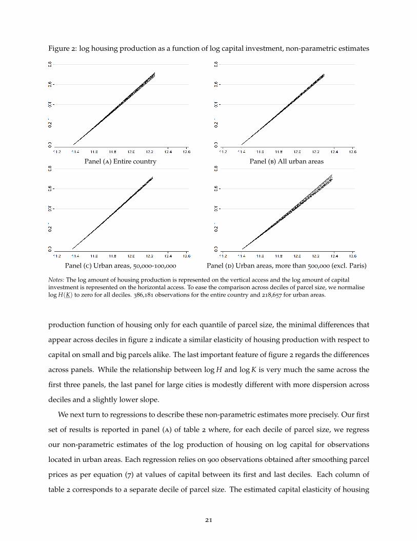
Figure 2: log housing production as a function of log capital investment, non-parametric estimates

Panel (a) Entire country Panel (b) All urban areas

Panel (c) Urban areas, 50,000-100,000 Panel (d) Urban areas, more than 500,000 (excl. Paris)

Notes: The log amount of housing production is represented on the vertical access and the log amount of capitalinvestment is represented on the horizontal access. To ease the comparison across deciles of parcel size, we normaliselog H(K) to zero for all deciles. 386,181 observations for the entire country and 218,657 for urban areas.

production function of housing only for each quantile of parcel size, the minimal differences that

appear across deciles in figure 2 indicate a similar elasticity of housing production with respect to

capital on small and big parcels alike. The last important feature of figure 2 regards the differences

across panels. While the relationship between log H and log K is very much the same across the

first three panels, the last panel for large cities is modestly different with more dispersion across

deciles and a slightly lower slope.

We next turn to regressions to describe these non-parametric estimates more precisely. Our first

set of results is reported in panel (a) of table 2 where, for each decile of parcel size, we regress

our non-parametric estimates of the log production of housing on log capital for observations

located in urban areas. Each regression relies on 900 observations obtained after smoothing parcel

prices as per equation (7) at values of capital between its first and last deciles. Each column of

table 2 corresponds to a separate decile of parcel size. The estimated capital elasticity of housing

21

Table 2: log housing production in urban areas, OLS by parcel size decile

Decile 1 2 3 4 5 6 7 8 9

Panel (A)log (K) 0.768a 0.779a 0.780a 0.779a 0.782a 0.788a 0.790a 0.794a 0.796a

(0.00064) (0.00053) (0.00064) (0.00066) (0.00081) (0.0011) (0.0012) (0.0016) (0.0020)[0.00071] [0.00059] [0.00063] [0.00073] [0.00085] [0.0011] [0.0012] [0.0016] [0.0019]

R2 1.00 1.00 1.00 1.00 1.00 1.00 1.00 1.00 1.00Observations 900 900 900 900 900 900 900 900 900

Panel (B)log (K) 0.379a 0.282a 0.217a 0.274a 0.288a 0.367a 0.502a 0.480a 0.498a

(0.028) (0.022) (0.026) (0.031) (0.040) (0.052) (0.070) (0.084) (0.087)[0.030] [0.021] [0.024] [0.031] [0.040] [0.051] [0.065] [0.082] [0.090]

[log (K)]2 0.016a 0.021a 0.024a 0.021a 0.021a 0.018a 0.012a 0.013a 0.013a

(0.0012) (0.00092) (0.0011) (0.0013) (0.0017) (0.0022) (0.0030) (0.0034) (0.0037)[0.00125] [0.00088] [0.00100] [0.0013] [0.0017] [0.0021] [0.0028] [0.0035] [0.0038]

R2 1.00 1.00 1.00 1.00 1.00 1.00 1.00 1.00 1.00Observations 900 900 900 900 900 900 900 900 900

Notes: OLS regressions with a constant in all columns. Bootstrapped standard errors with 100 bootstraps inparentheses and with 1,000 bootstraps in squared parentheses. a, b, c: significant at 1%, 5%, 10%.Non-parametric estimates of housing production rely on 218,657 observations.

for the first decile is 0.77. It is 0.78 for the second to the fifth decile, 0.79 for the seventh and

eighth, and finally 0.80 for the last decile. While these elasticities are not exactly constant across

deciles, the differences remain small. Interestingly, the capital elasticity of housing is estimated

to be larger in larger parcels. This is consistent with the production function of housing being

log super-modular. For a constant-elasticity of substitution production function, this implies land

and capital being (weakly) complement and an elasticity of substitution between land and capital

just below one. Because these estimates are subject to a number of identification worries, we

refrain from further conclusions for now but note that the differences in the production function

across parcels of different sizes are economically small. Importantly, we also note that our linear

regressions provide a near perfect fit as the R2 is always above 0.999.34

Panel (b) of table 2 replicates the regressions of panel (a) adding the square of log capital as

explanatory variable. We note that the estimated coefficient of the quadratic term is significant

in all regressions with a coefficient between 0.012 and 0.024. Hence, the production function for

34Recall that we work with smoothed data, which condition out idiosyncratic variation. To be clear, this R2 does notmeasure how well our regression fits the raw data but how well the functional form imposed by the regression fits thenon-parametric estimate of the housing production function.

22

Table 3: log housing production, OLS by class of urban area population

City size class Country Urban 0-50 50-100 100-200 200-500 500+ Parisareas

Panel (A)log (K) 0.805a 0.784a 0.832a 0.822a 0.814a 0.785a 0.730a 0.700a

(0.00060) (0.00063) (0.0014) (0.0012) (0.0011) (0.0011) (0.0014) (0.0025)

Panel (B)log (K) 0.315a 0.365a -0.075a 0.038a 0.230a 0.068a -0.091a -0.002

(0.028) (0.025) (0.062) (0.052) (0.039) (0.038) (0.050) (0.070)

[log (K)]2 0.021a 0.018a 0.038a 0.033a 0.025a 0.030a 0.034a 0.029a

(0.0018) (0.0011) (0.0026) (0.0022) (0.0017) (0.0016) (0.0021) (0.0028)

Notes: OLS regressions with decile fixed effects in all columns. 8,100 observations for each regression. TheR2 is 1.00 in all specifications. Bootstrapped standard errors in parentheses. a, b, c: significant at 1%, 5%,10%.

housing is not strictly log linear in capital but log convex. Because log capital typically varies

between about 11.4 at the bottom decile and, 12.2 at the top decile, this log convexity implies that

the capital elasticity of housing is only about 0.02 larger for houses built at the top decile of capital

relative to houses built at the bottom decile. While the housing production function is log convex,

this log convexity is minimal and the differences in the capital elasticity between the largest and

smallest houses are tiny.

All the coefficients reported in table 2 are highly significant. This table reports two series

of standard errors with 100 and 1,000 bootstraps, respectively. Because taking 1,000 bootstraps

does not make any substantive difference and because these bootstraps are computationally very

intensive, we only report standard errors computed from 100 bootstraps in what follows.

Panel (a) of table 3 regresses again the log of estimated housing production on log capital but

this time considers different samples of new constructions corresponding to different geographies.

In each regression, all the parcel size deciles are lumped together and decile fixed effects are

included. The first column considers the entire population of transactions. The estimated capital

elasticity of housing is 0.80. Column 2 considers only observations from urban areas and estimates

a marginally lower elasticity of 0.78. The following six columns consider urban areas of increasing

sizes. For the smallest urban areas with population below 50,000 the estimated capital elasticity

is 0.83. This elasticity is 0.73 for large urban areas with population above 500,000 and 0.70 for

Paris. Because land is more expensive in larger cities, these results are again consistent with a

23

modest complementarity between land and capital in the production of housing. Panel (b) of table

3 repeats the same exercise as panel (a) adding a quadratic term for log capital. Just like panel (b)

of table 2 it provides evidence of a modest log convexity.

Before turning to our results based on predicted land prices and capital, we assess the robust-

ness of the results we have obtained so far through four different checks. First, recall that houses

are built for specific buyers who may have idiosyncratic preferences that affect construction costs.

Because the information about construction costs is for one of three levels of completion, we can

compare results across these levels of completion (fully finished units, ready-to-decorate units,

and units with only a completed structure). Any unobserved heterogeneity associated with the

customisation of houses should have a greater effect on fully finished units than on bare-bone

structures. Table 11 in Appendix C duplicates panel (a) of table 2 but splits observations by level

of completion. Unsurprisingly, we find a slightly higher capital elasticity for more finished houses

that reflects their greater capital intensity. For the median parcel, the capital elasticity is 0.793 for

fully finished units, 0.779 for ready-to-decorate units, and 0.755 for units with only a completed

structure. The corresponding elasticity in table 2 is 0.782. Importantly, for all levels of completion,

we find again a modestly increasing capital elasticity as we consider higher parcel size deciles as

in table 2.

The segmentation of housing markets may imply another form of unobserved heterogeneity.

While we cannot track the heterogeneity of houses directly, it may be reflected in the heterogeneity

of buyers. We can use information regarding the buyer’s occupation and split the sample of trans-

actions by buyers’ occupation: executives, intermediate occupations, and clerical and blue-collar

workers. We report results for these three groups in table 12 in Appendix C. The differences

between occupational categories are small. For the median parcel, the capital elasticity is 0.771

for executives, 0.781 for intermediate occupations, and 0.791 for clerical and blue-collar workers

with the same general pattern of modestly increasing elasticities as we consider larger parcels.

As noted above, the details of our smoothing procedure affects the quality of our predictions

for land prices. To verify that our results are not affected by our choice of bandwidth, table 13

in Appendix C repeats the estimations of table 2 for bandwidths equal to a half, a quarter, and

a tenth of the rule-of-thumb bandwidth, respectively. When regressing log housing production

on log capital, the results are virtually identical for all bandwidths. When we also include the

square of log capital as explanatory variable, the results are again the same except, perhaps, for

24

the smallest bandwidth at the top decile of parcel sizes.35 Reassuringly, these results show that we

need to consider extreme forms of under-smoothing before running into these problems. The main

conclusion is that our results are not affected by our choice of bandwidth.

Finally, table 14 in Appendix C duplicates again table 2 but does not apply our user cost

correction of 6% for structure and 3% for land. Because we no longer account for the depreciation

of capital and the appreciation of land, we estimate a lower coefficient on capital to 0.642 for the

median parcel. This elasticity should now be interpreted as the elasticity of the housing stock

instead of the elasticity of housing services. The lack of user cost correction does not affect our

results beyond this re-scaling and a slight difference in interpretation.

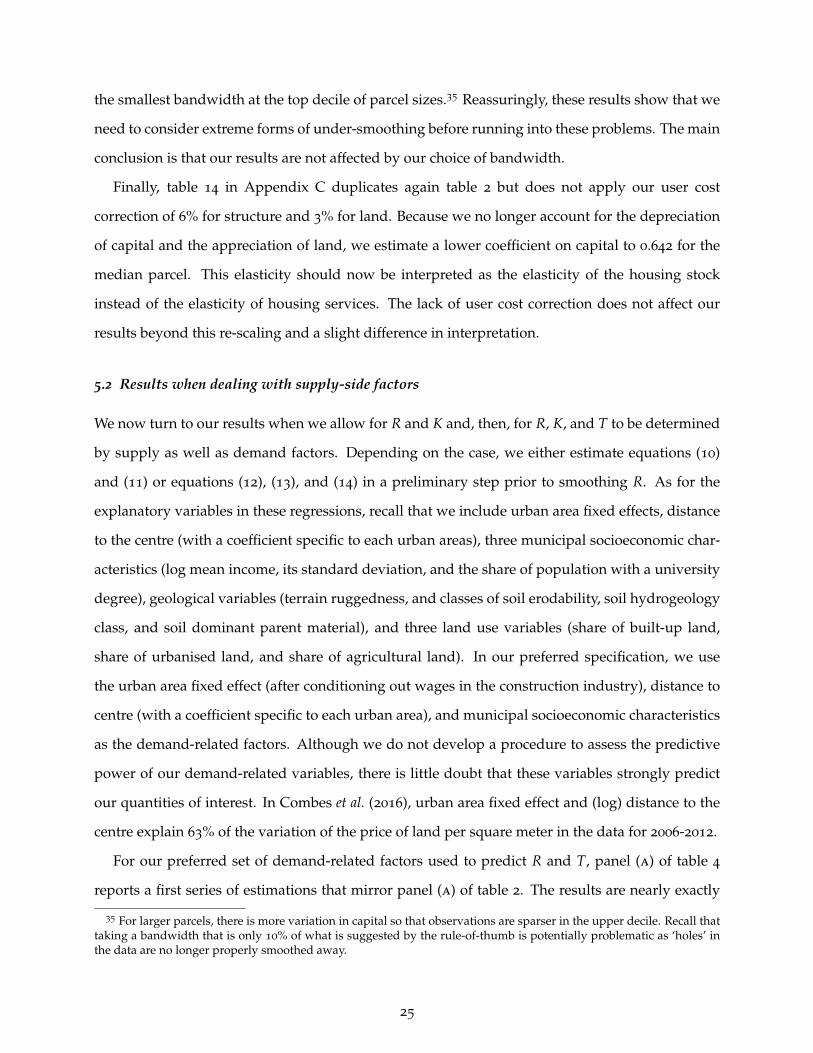
5.2 Results when dealing with supply-side factors

We now turn to our results when we allow for R and K and, then, for R, K, and T to be determined

by supply as well as demand factors. Depending on the case, we either estimate equations (10)

and (11) or equations (12), (13), and (14) in a preliminary step prior to smoothing R. As for the

explanatory variables in these regressions, recall that we include urban area fixed effects, distance

to the centre (with a coefficient specific to each urban areas), three municipal socioeconomic char-

acteristics (log mean income, its standard deviation, and the share of population with a university

degree), geological variables (terrain ruggedness, and classes of soil erodability, soil hydrogeology

class, and soil dominant parent material), and three land use variables (share of built-up land,

share of urbanised land, and share of agricultural land). In our preferred specification, we use

the urban area fixed effect (after conditioning out wages in the construction industry), distance to

centre (with a coefficient specific to each urban area), and municipal socioeconomic characteristics

as the demand-related factors. Although we do not develop a procedure to assess the predictive

power of our demand-related variables, there is little doubt that these variables strongly predict

our quantities of interest. In Combes et al. (2016), urban area fixed effect and (log) distance to the

centre explain 63% of the variation of the price of land per square meter in the data for 2006-2012.

For our preferred set of demand-related factors used to predict R and T, panel (a) of table 4

reports a first series of estimations that mirror panel (a) of table 2. The results are nearly exactly

35 For larger parcels, there is more variation in capital so that observations are sparser in the upper decile. Recall thattaking a bandwidth that is only 10% of what is suggested by the rule-of-thumb is potentially problematic as ‘holes’ inthe data are no longer properly smoothed away.

25

Table 4: log housing production in urban areas obtained from predicted values of variables, OLS

by parcel size decile

Decile 1 2 3 4 5 6 7 8 9

Panel (A): Predicted R and Klog (K) 0.784a 0.786a 0.787a 0.789a 0.793a 0.799a 0.803a 0.807a 0.812a

(0.00082) (0.00049) (0.00039) (0.00051) (0.00065) (0.00085) (0.0011) (0.0012) (0.0014)

Panel (B): Predicted R and Klog (K) 0.383a 1.008a 1.510a 1.851a 1.967a 1.929a 1.602a 1.507a 1.664a

(0.101) (0.064) (0.054) (0.059) (0.072) (0.098) (0.126) (0.145) (0.160)

[log (K)]2 0.017a -0.009a -0.031a -0.045a -0.050a -0.048a -0.034a -0.030a -0.036a

(0.0043) (0.0027) (0.0023) (0.0025) (0.0030) (0.0041) (0.0053) (0.0061) (0.0068)

Panel (C): Predicted R, K, and Tlog (K) 0.789a 0.798a 0.791a 0.790a 0.788a 0.784a 0.786a 0.798a 0.807a

(0.0017) (0.0012) (0.0017) (0.0016) (0.0019) (0.0020) (0.0025) (0.0021) (0.0026)

Panel (D): Predicted R, K, and Tlog (K) 0.311 0.849a 1.080a 2.007a 2.796a 2.536a 2.791a 2.098a 1.938a

(0.260) (0.179) (0.282) (0.252) (0.362) (0.327) (0.367) (0.297) (0.350)

[log (K)]2 0.020c -0.002 -0.012 -0.051a -0.085a -0.074a -0.085a -0.055a -0.048a

(0.011) (0.0076) (0.012) (0.011) (0.015) (0.014) (0.016) (0.013) (0.015)

Notes: OLS regressions with a constant in all columns. 900 observations for each regression. The R2 is 1.00in all specifications. Capital and parcel price are constructed using urban area fixed effects (afterconditioning out construction wages), distance to the centre (urban-area specific), and income variables(log mean municipal income, log standard error of income, and share of population with a universitydegree). For parcel size, observed values are used in panels (A) and (B), and values predicted from thesame variables as capital and parcel price are used in panels (C) and (D). Bootstrapped standard errors inparentheses. a, b, c: significant at 1%, 5%, 10%. Non-parametric estimates of housing production rely on213,788 observations (instead of 218,657 when we do not use predicted values of land prices and capital).

the same with a similar pattern of increasing elasticity of housing production with respect to

capital as higher deciles of parcel size are considered. The only difference is that the elasticities are

marginally higher than those in table 2. Even though the estimated differences in elasticity across

the two tables for the same decile of parcel area in panel (a) are significant in a statistical sense,

they are economically tiny since the difference is always less than 0.013 for elasticities around 0.8.

Panel (b) of table 4 adds a quadratic term for log K and duplicates the specifications of the

corresponding panel of table 2. The results now indicate the presence of a mild log concavity for

all deciles of parcel size except the first one. This is in contrast with table 2 where the results point

towards modest log convexity. While there is some variation in the estimated coefficient on the

quadratic term in log K across deciles of parcel size, the largest one in absolute value is 0.05 for the

26

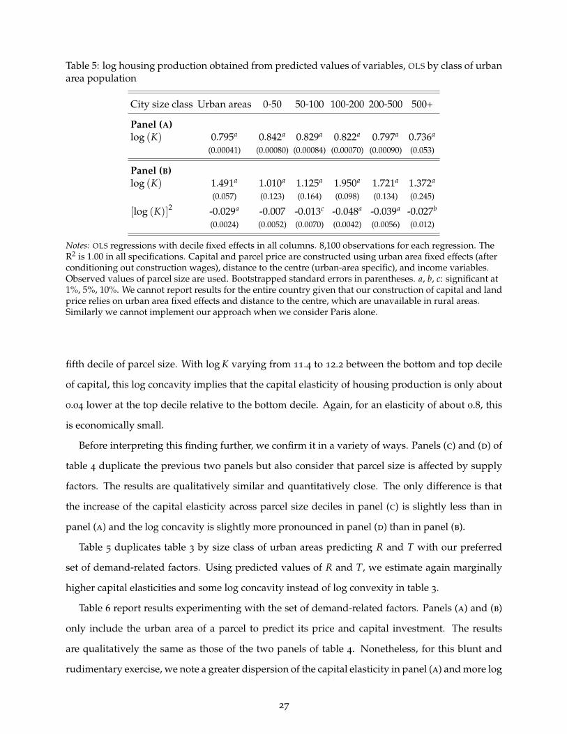
Table 5: log housing production obtained from predicted values of variables, OLS by class of urbanarea population

City size class Urban areas 0-50 50-100 100-200 200-500 500+

Panel (A)log (K) 0.795a 0.842a 0.829a 0.822a 0.797a 0.736a

(0.00041) (0.00080) (0.00084) (0.00070) (0.00090) (0.053)

Panel (B)log (K) 1.491a 1.010a 1.125a 1.950a 1.721a 1.372a

(0.057) (0.123) (0.164) (0.098) (0.134) (0.245)

[log (K)]2 -0.029a -0.007 -0.013c -0.048a -0.039a -0.027b

(0.0024) (0.0052) (0.0070) (0.0042) (0.0056) (0.012)

Notes: OLS regressions with decile fixed effects in all columns. 8,100 observations for each regression. TheR2 is 1.00 in all specifications. Capital and parcel price are constructed using urban area fixed effects (afterconditioning out construction wages), distance to the centre (urban-area specific), and income variables.Observed values of parcel size are used. Bootstrapped standard errors in parentheses. a, b, c: significant at1%, 5%, 10%. We cannot report results for the entire country given that our construction of capital and landprice relies on urban area fixed effects and distance to the centre, which are unavailable in rural areas.Similarly we cannot implement our approach when we consider Paris alone.

fifth decile of parcel size. With log K varying from 11.4 to 12.2 between the bottom and top decile

of capital, this log concavity implies that the capital elasticity of housing production is only about

0.04 lower at the top decile relative to the bottom decile. Again, for an elasticity of about 0.8, this

is economically small.

Before interpreting this finding further, we confirm it in a variety of ways. Panels (c) and (d) of

table 4 duplicate the previous two panels but also consider that parcel size is affected by supply

factors. The results are qualitatively similar and quantitatively close. The only difference is that

the increase of the capital elasticity across parcel size deciles in panel (c) is slightly less than in

panel (a) and the log concavity is slightly more pronounced in panel (d) than in panel (b).

Table 5 duplicates table 3 by size class of urban areas predicting R and T with our preferred

set of demand-related factors. Using predicted values of R and T, we estimate again marginally

higher capital elasticities and some log concavity instead of log convexity in table 3.

Table 6 report results experimenting with the set of demand-related factors. Panels (a) and (b)

only include the urban area of a parcel to predict its price and capital investment. The results

are qualitatively the same as those of the two panels of table 4. Nonetheless, for this blunt and

rudimentary exercise, we note a greater dispersion of the capital elasticity in panel (a) and more log

27

concavity, especially for the lower deciles of parcel size in panel (b). Panels (c) and (d) rely again on

the urban area of a parcel to predict its price and capital investment but condition out local wages

in the construction industry from the estimated urban area fixed effects. With this specification, the

differences in capital elasticity across parcel size deciles are minimal. Depending on the deciles,

the production function of housing is either mildly log concave or mildly log convex. Panels (e)

and (f) include urban area fixed effects, distance to the centre (with an effect specific to each urban

area), income, and land-use variables among the demand determinants but do not condition out

construction wages. Finally, panels (g) and (h) additionally condition out construction wages from

urban area fixed effects and predict parcel size with demand-related factors. Although one may

(rightfully) object that land use patterns may reflect more than just local demand conditions (even

after conditioning out geological characteristics), the similarity with the results of table 4 shows

that our results when using predicted quantities are not sensitive to the exact details of what we

include in our set of demand-related factors.

Overall our results when using predicted quantities suggest a marginally higher elasticity of

housing production with respect to capital. The difference is nonetheless too small to be econom-

ically meaningful. More importantly, our results when using predicted quantities indicate that

the production function for housing is mildly log concave rather than log convex when using raw

quantities. This change makes intuitive sense in relation to the possible biases described above. For

parcels of the same area, we expect parcels that are more difficult to build to require more capital.

The price of these parcels will also be lower due to this. With lower prices for parcels receiving a

greater capital investment, the share of capital will thus increase with the amount of capital used

to build the house (all else equal). This can bias our results and generate an apparent log convexity

of the production of housing when we do not control for supply factors.

28

Table 6: log housing production in urban areas obtained from predicted values of variables, OLS


Decile 1 2 3 4 5 6 7 8 9

Panel (A): Urban area fixed effects onlylog (K) 0.755a 0.775a 0.788a 0.796a 0.802a 0.810a 0.816a 0.820a 0.824a

(0.0017) (0.0017) (0.0011) (0.00088) (0.0011) (0.0013) (0.0015) (0.0015) (0.0019)

Panel (B): Urban area fixed effects onlylog (K) 4.760a 4.437a 2.934a 2.271a 2.410a 2.422a 2.395a 2.387a 2.580a

(0.294) (0.187) (0.200) (0.134) (0.174) (0.207) (0.224) (0.254) (0.308)

[log (K)]2 -0.169a -0.155a -0.091a -0.062a -0.068a -0.068a -0.067a -0.066a -0.074a

(0.012) (0.0080) (0.0085) (0.0056) (0.0074) (0.0088) (0.0095) (0.011) (0.013)

Panel (C): Urban area fixed effects net of construction wageslog (K) 0.789a 0.780a 0.776a 0.775a 0.776a 0.778a 0.779a 0.781a 0.787a

(0.0026) (0.00080)(0.00065)(0.00074)(0.00093) (0.0015) (0.0022) (0.0028) (0.0045)

Panel (D): Urban area fixed effects net of construction wageslog (K) -0.523 -0.126 0.824a 1.244a 1.385a 1.061a 0.194 -0.174 0.661

(0.441) (0.150) (0.138) (0.115) (0.172) (0.324) (0.480) (0.645) (0.948)

[log (K)]2 0.055a 0.038a -0.002a -0.020a -0.026a -0.012 0.025 0.040 0.005(0.019) (0.0063) (0.0058) (0.0049) (0.0073) (0.014) (0.020) (0.027) (0.040)

Panel (E): Urban area fixed effects, distance effects, income, and land uselog (K) 0.761a 0.775a 0.782a 0.788a 0.795a 0.803a 0.808a 0.814a 0.821a

(0.00096)(0.00064)(0.00051)(0.00056)(0.00081) (0.0010) (0.0011) (0.0014) (0.0017)

Panel (F): Urban area fixed effects, distance effects, income, and land uselog (K) 3.209a 2.958a 2.919a 3.045a 3.194a 3.270a 3.332a 3.258a 3.175a

(0.066) (0.059) (0.054) (0.057) (0.060) (0.069) (0.076) (0.106) (0.123)

[log (K)]2 -0.103a -0.092a -0.090a -0.095a -0.101a -0.104a -0.107a -0.103a -0.099a

(0.0028) (0.0025) (0.0023 (0.0024) (0.0026) (0.0029) (0.0032) (0.0045) (0.0053)

Panel (G): ——– net of construction wages with predicted Tlog (K) 0.779a 0.786a 0.790a 0.787a 0.790a 0.793a 0.792a 0.805a 0.813a

(0.0014) (0.0012) (0.0014) (0.0016) (0.0011) (0.0016) (0.0021) (0.0022) (0.0024)

Panel (H): ——– net of construction wages with predicted Tlog (K) -0.270 1.192a 2.409a 2.741a 2.668a 2.152a 2.418a 1.930a 1.426a

(0.240) (0.202) (0.229) (0.222) (0.195) (0.167) (0.230) (0.276) (0.290)

[log (K)]2 0.044a -0.017b -0.068a -0.082a -0.079a -0.057a -0.069a -0.047a -0.026b

(0.010) (0.0085) (0.0097) (0.0094) (0.0083) (0.0071) (0.0098) (0.012) (0.012)

Notes: OLS regressions with a constant in all columns. In all panels (E)-(H), distance to the centre isurban-area specific; income variables are log mean municipal income, log standard error of income, andshare of population with a university degree; geology variables are ruggedness, soil erodability, soilhydrogeological class, dominant parent material for two main classes of (lighter) soils; land use variablesare three land use variables share of built-up land , share of urbanised land, and share of agricultural land.900 observations for each regression. The R2 is 1.00 in all specifications. Robust standard errors inparentheses. a, b, c: significant at 1%, 5%, 10%.

29

6. Recovering a functional form

So far, we have non-parametrically estimated the production of housing as a function of capital,

given parcel size. We then estimated simple regressions to assess the shape of this non-parametric

function. As a first approximation, the production function of housing is log linear with a share of

capital of about 0.80. However, a more detailed look suggests mild log convexity when using the

raw data and, perhaps more reasonably, modest log concavity with predicted values of land prices

and capital.

In this section, we asses a variety of functional forms for the production function of housing.

Given our results, measuring the goodness of fit of different specifications is unlikely to be in-

formative since the simplest log linear specifications always have an R2 close to unity. Instead,

we duplicate our estimation of the capital elasticity of housing production for each decile of

parcel size, having imposed specific functional forms for the production of housing instead of

doing it non-parametrically. We can then compare the results we obtain using these (pre-imposed)

functional forms to our earlier, non-parametric estimations results.

For the exposition to remain concrete, consider a ces production function. The production

of housing is given by H = A(

αK(σ−1)/σ + (1− α)T(σ−1)/σ)σ/(σ−1)

where σ is the elasticity of

substitution between land and capital and A is a productivity shifter. Using equation (4) and the

partial derivative of the ces production function with respect to K, we obtain the following cost

share:rK∗

rK∗ + R(K∗,T)=

α(K∗)1−1/σ

α(K∗)1−1/σ + (1− α)T1−1/σ. (15)

From values on a 300 × 300 grid, we can estimate α and σ using equation (15) by minimising

the sum of the squared distances between estimated costs shares and those predicted by a ces

production function.36 We then compute “ces productions” of housing at the points of our grid

using the estimated parameters and perform the same regression as in table 2. We also repeat the

same exercise using predicted by demand-related factors as in table 4. Aside from the ces, we also

make an assessment for the Cobb-Douglas and for the second- and third-order translog production

functions.36We weigh observations with the kernel weights used for determining the land price on the grid to take into account

the distribution of observations in the data.

30

Table 7: log housing production fitting specific functional forms, OLS by parcel size decile

Decile 1 2 3 4 5 6 7 8 9

Panel (A): Cobb-Douglaslog (K) 0.776a 0.776a 0.776a 0.776a 0.776a 0.776a 0.776a 0.776a 0.776a

(0.00054) (0.00054) (0.00054) (0.00054) (0.00054) (0.00054) (0.00054) (0.00054) (0.00054)

Panel (B): Cobb-Douglaslog (K) 0.776a 0.776a 0.776a 0.776a 0.776a 0.776a 0.776a 0.776a 0.776a

(0.00054) (0.00054) (0.00054) (0.00054) (0.00054) (0.00054) (0.00054) (0.00054) (0.00054)

[log (K)]2 2.17e-7 -1.45e-7 -1e-7 -1.56e-7 -1.62e-7 -1.08e-7 -2.02e-7 -0.99e-7 -1.25e-7(1.7e-7) (1.5e-7) (1.5e-7) (1.3e-7) (1.5e-7) (1.4e-7) (1.5e-7) (1.5e-7) (1.6e-7)

Panel (C): CESlog (K) 0.762a 0.767a 0.770a 0.773a 0.776a 0.778a 0.780a 0.781a 0.783a

(0.00057) (0.00057) (0.00057) (0.00057) (0.00056) (0.00056) (0.00056) (0.00056) (0.00056)

Panel (D): CESlog (K) 0.928a 0.935a 0.939a 0.943a 0.946a 0.948a 0.951a 0.952a 0.954a

(0.00084) (0.00085) (0.00085) (0.00086) (0.00086) (0.00086) (0.00086) (0.00087) (0.00087)

[log (K)]2 -0.0070a -0.0070a -0.0071a -0.0071a -0.0072a -0.0072a -0.0072a -0.0072a -0.0072a

(0.00003) (0.00003) (0.00003) (0.00003) (0.00003) (0.00003) (0.00003) (0.00003) (0.00003)

Panel (E): Second-order transloglog (K) 0.771a 0.775a 0.778a 0.781a 0.783a 0.785a 0.786a 0.788a 0.789a

(0.00072) (0.00057) (0.00053) (0.00054) (0.00059) (0.00065) (0.00071) (0.00077) (0.00083)

Panel (F): Second-order transloglog (K) 0.184a 0.188a 0.191a 0.193a 0.195a 0.197a 0.199a 0.200a 0.201a

(0.015) (0.015) (0.015) (0.015) (0.015) (0.016) (0.016) (0.016) (0.016)

[log (K)]2 0.0247a 0.0247a 0.0247a 0.0247a 0.0247a 0.0247a 0.0247a 0.0247a 0.0247a

(0.00065) (0.00065) (0.00065) (0.00065) (0.00065) (0.00065) (0.00065) (0.00065) (0.00065)

Panel (G): Third-order transloglog (K) 0.775a 0.777a 0.779a 0.781a 0.784a 0.787a 0.789a 0.792a 0.794a

(0.00084) (0.00060) (0.00063) (0.00060) (0.00058) (0.00067) (0.00087) (0.0011) (0.0014)

Panel (H): Third-order transloglog (K) 0.257a 0.272a 0.284a 0.295a 0.304a 0.312a 0.320a 0.327a 0.333a

(0.026) (0.018) (0.016) (0.017) (0.022) (0.026) (0.030) (0.034) (0.037)

[log (K)]2 0.0218a 0.0212a 0.0208a 0.0205a 0.0202a 0.0200a 0.0198a 0.0196a 0.0194a

(0.0011) (0.00076) (0.00069) (0.00078) (0.00094) (0.0011) (0.0013) (0.0014) (0.0016)

Notes: OLS regressions with a constant in all columns. 900 observations for each regression. The R2 is 1.00in all specifications. Bootstrapped standard errors in parentheses. a, b, c: significant at 1%, 5%, 10%. For thesecond-order translog, there is a single coefficient for all deciles of parcel size for the term in log K squaredby definition.

31

Table 7 reports a first series of results using raw data. In panel (a) of table 7, we can see

that imposing Cobb-Douglas to the data leads to about the same capital elasticities of housing

production as in table 2 but, by construction, this fails to replicate the higher elasticity for larger

parcels. By construction again, the capital elasticity of 0.776 that we recover is the same as the one

estimated from factor shares. Panel (b) also includes a quadratic term for log K and estimates, as

expected, the same coefficient of 0.776 for log K and a coefficient of 0 (or extremely close to) for its

square.

For the ces case, we note that the estimated parameter values for the production function are

α = 0.794 and σ = 0.902. This value of σ close to one implies a situation close to the Cobb-Douglas

case. In panel (c), the coefficients on log K are, unsurprisingly, very close to those estimated in the

Cobb-Douglas case except that this panel also replicates the tendency of the capital elasticity to

increase with parcel size. In panel (d), we estimate minimal log concavity in capital instead of the

log convexity reported in panel (b) of table 2. In panel (e), the second-order translog is also able

to replicate the upward trend in the capital elasticity. These elasticities are about equal to those

reported in table 2. In panel (f), the coefficients on the quadratic term in log capital reproduce,

albeit more strongly, the log convexity in capital estimated in table 2. Panels (g) and (h) report

results for a third-order translog function instead of a second-order translog. The results match

those obtained in table 2 marginally better than those of the second-order translog.

Table 8 repeats the same exercise for values of K and R predicted from demand-related factors

instead of the observed values used in table 7. The results should now be compared with those of

table 4. Again, the Cobb-Douglas specification delivers capital elasticities of the right magnitude

but is obviously unable to generate the log concavity estimated in panel (b) of table 4. The ces

specification is able to reproduce both the tendency of the capital elasticity to be higher in higher

deciles of parcel size in panel (c) and the estimated log concavity of H in K when adding a

quadratic term in panel (d). The elasticity of substitution between land and capital estimated from

the data is 0.795, which is somewhat different from the elasticity of 0.902 estimated above when

using observed values. The amount of concavity obtained from the ces specification is tiny and

slightly less than what is estimated in table 4. The two translog specifications in panels (e)-(h) can

match closely the capital elasticities estimated in table 4 and replicate the log concavity of H in K.

For the specification that includes squared log capital, the third-order translog of panel (h) offers

32

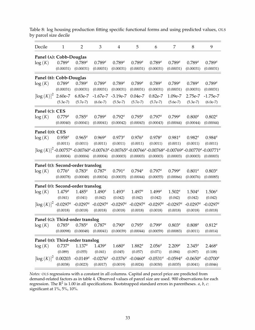
Table 8: log housing production fitting specific functional forms and using predicted values, OLS


Decile 1 2 3 4 5 6 7 8 9

Panel (A): Cobb-Douglaslog (K) 0.789a 0.789a 0.789a 0.789a 0.789a 0.789a 0.789a 0.789a 0.789a

(0.00031) (0.00031) (0.00031) (0.00031) (0.00031) (0.00031) (0.00031) (0.00031) (0.00031)

Panel (B): Cobb-Douglaslog (K) 0.789a 0.789a 0.789a 0.789a 0.789a 0.789a 0.789a 0.789a 0.789a

(0.00031) (0.00031) (0.00031) (0.00031) (0.00031) (0.00031) (0.00031) (0.00031) (0.00031)

[log (K)]2 2.60e-7 6.83e-7 -1.67e-7 -3.19e-7 0.04e-7 0.82e-7 1.09e-7 2.75e-7 -1.75e-7(5.3e-7) (5.7e-7) (6.0e-7) (5.5e-7) (5.7e-7) (5.7e-7) (5.6e-7) (5.3e-7) (6.0e-7)

Panel (C): CESlog (K) 0.779a 0.785a 0.789a 0.792a 0.795a 0.797a 0.799a 0.800a 0.802a

(0.00040) (0.00041) (0.00041) (0.00042) (0.00043) (0.00043) (0.00044) (0.00044) (0.00044)

Panel (D): CESlog (K) 0.958a 0.965a 0.969a 0.973a 0.976a 0.978a 0.981a 0.982a 0.984a

(0.0011) (0.0011) (0.0011) (0.0011) (0.0011) (0.0011) (0.0011) (0.0011) (0.0011)

[log (K)]2 -0.00757a -0.00760a -0.00763a -0.00765a -0.00766a -0.00768a -0.00769a -0.00770a -0.00771a

(0.00004) (0.00004) (0.00004) (0.00003) (0.00003) (0.00003) (0.00003) (0.00003) (0.00003)

Panel (E): Second-order transloglog (K) 0.776a 0.783a 0.787a 0.791a 0.794a 0.797a 0.799a 0.801a 0.803a

(0.00078) (0.00048) (0.00034) (0.00035) (0.00044) (0.00055) (0.00066) (0.00076) (0.00085)

Panel (F): Second-order transloglog (K) 1.479a 1.485a 1.490a 1.493a 1.497a 1.499a 1.502a 1.504a 1.506a

(0.041) (0.041) (0.042) (0.042) (0.042) (0.042) (0.042) (0.042) (0.042)

[log (K)]2 -0.0297a -0.0297a -0.0297a -0.0297a -0.0297a -0.0297a -0.0297a -0.0297a -0.0297a

(0.0018) (0.0018) (0.0018) (0.0018) (0.0018) (0.0018) (0.0018) (0.0018) (0.0018)

Panel (G): Third-order transloglog (K) 0.785a 0.785a 0.787a 0.790a 0.795a 0.799a 0.803a 0.808a 0.812a

(0.00098) (0.00048) (0.00041) (0.00039) (0.00044) (0.00059) (0.00083) (0.0011) (0.0014)

Panel (H): Third-order transloglog (K) 0.737a 1.137a 1.439a 1.680a 1.882a 2.056a 2.209a 2.345a 2.468a

(0.089) (0.055) (0.041) (0.045) (0.057) (0.071) (0.084) (0.097) (0.108)

[log (K)]2 0.00203 -0.0149a -0.0276a -0.0376a -0.0460a -0.0531a -0.0594a -0.0650a -0.0700a

(0.0038) (0.0023) (0.0017) (0.0019) (0.0024) (0.0030) (0.0035) (0.0041) (0.0046)

Notes: OLS regressions with a constant in all columns. Capital and parcel price are predicted fromdemand-related factors as in table 4. Observed values of parcel size are used. 900 observations for eachregression. The R2 is 1.00 in all specifications. Bootstrapped standard errors in parentheses. a, b, c:significant at 1%, 5%, 10%.

33

the best match with the results of table 4 obtained with predicted values.

We draw three conclusions from this section. First, we confirm that a Cobb-Douglas specifi-

cation provides a good first-order description of the data. Second, and consistent with this, we

find that the estimation of a ces production function for housing has an elasticity of substitution

between land and capital inputs of 0.8 to 0.9 depending on whether or not we predict quantities

with demand-related factors. The ces provides a better description of the predicted data but the

gain relative to a Cobb-Douglas specification is small. Overall, the third-order translog offers the

closest approximation to our non-parametric results but the gain from this more flexible functional

form is again small. Third, none of the functional form we consider is able to match exactly the

results of our non-parametric estimation. Put differently, these results suggest that it is better to

use a non-parametric approach and then provide an functional form approximation than impose

a functional form directly into the estimation.

7. Full identification?

In our approach so far, we have assumed that parcels were taken as given by house builders. We

think that taking parcels as exogenous is reasonable in the French institutional context. Recall that

our data pertain to single-family homes built mostly individually (or in small numbers) as in-fills.

This said, it is easy to expand the model-based approach developed in section 2 and allow for

house builders to maximise their profits with respect to both capital and parcel size. This extension

is fully developed in Appendix D.

We assume that land rent is linear in land area R = R(x)× T, in which case the unit price of

land is constant at a given location regardless of parcel size. This assumption is natural in a context

of divisible land and competitive land-owners. It prevents any arbitrage gain from re-selling part

of parcels that would have been bought at lower unit prices. A second argument in the profit

function of house builders introduces a second first-order condition. Importantly, for the two first-

order conditions of the builder’s problem to be consistent with zero profit, the housing production

function is necessarily constant returns to scale.

Substituting both first-order conditions into the zero profit condition allows us to fully identify

the production function of housing. This is in contrast with our partially identified approach so

far. To assess whether imposing constant returns to scale is warranted, we perform two checks.

34

Table 9: Explaining the price of land per square metre

(1) (2) (3) (4) (5) (6) (7) (8)Dependent variable Raw data Smoothed data

Log parcel size -0.991a -0.971a -0.759a -0.644a -0.656a 0.922a -1.084a -0.254a

(0.002) ( 0.003) (0.002) (0.002) (0.002) (0.024) (0.001) (0.063)

Log parcel size squared -0.114a -0.060a

(0.002) (0.005)

Parcel controls No Yes Yes Yes Yes Yes No NoUrban area indicator No No Yes Yes Yes Yes No NoDistance to the centre No No No Yes Yes Yes No NoMunicipal controls No No No No Yes Yes No No

Observations 213,788 213,788 213,788 213,788 213,788 213,788 90,000 90,000R2 0.43 0.45 0.74 0.79 0.80 0.81 0.81 0.81

Note OLS regressions with year effects in all columns. a: significant at 1% level; b: significant at 5% level; a: significant at 10% level. Parcelcontrols include indicator variables for whether the parcel is serviced and three types of intermediaries through whom the parcel may havebeen bought. Municipal controls include log area, log mean income of the year, log standard error of income of the year, share of municipalland that is urbanised (covered) in 2006, share of municipal land for agriculture, ruggedness, soil erodability, soil hydrogeological class,dominant parent material for two main classes of (lighter) soils.

First, we regress the log of the price of parcels per unit of land R(x) on log parcel size and

other parcel characteristics. The results are reported table 9. Column 1 regresses the log price of

parcels per square metre on the log of their size. Strikingly, the coefficient is about minus one.

Adding parcel controls, urban area indicators, distance to the centre (with a coefficient specific

to each urban area), and many municipal controls in columns 2 to 5 lowers the magnitude of

the coefficient on log parcel size. Nonetheless, even with a full set of controls, the coefficient on

parcel size remains large in magnitude at about -0.66.37 Adding a quadratic term on log parcel size

in column 6 provides evidence of some log concavity indicating that the marginal price of land

declines faster for larger parcels. Columns 7 and 8 use kernel-smoothed land price data instead

of the actual transaction price data used in columns 1 to 6. The results in these last two columns

essentially confirm the result that unit land prices strongly decline with parcel size. When builders

are able to maximise profits with respect to parcel size, the unit price of land should be equalised

across parcels of different sizes. Our results clearly reject this prediction.

For our second exercise, we proceed in the spirit of what we do in section 6 and re-estimate

housing production under the added restriction of constant returns to scale. We can then regress

the constant-return values of log H on log K. If imposing constant returns to scale was innocuous,

37For a very similar specification using us land price data, Albouy and Ehrlich (2013) estimate a coefficient of -0.61.

35

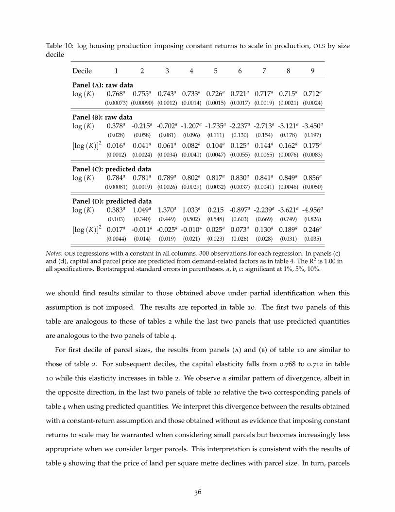
Table 10: log housing production imposing constant returns to scale in production, OLS by sizedecile

Decile 1 2 3 4 5 6 7 8 9

Panel (A): raw datalog (K) 0.768a 0.755a 0.743a 0.733a 0.726a 0.721a 0.717a 0.715a 0.712a

(0.00073) (0.00090) (0.0012) (0.0014) (0.0015) (0.0017) (0.0019) (0.0021) (0.0024)

Panel (B): raw datalog (K) 0.378a -0.215a -0.702a -1.207a -1.735a -2.237a -2.713a -3.121a -3.450a

(0.028) (0.058) (0.081) (0.096) (0.111) (0.130) (0.154) (0.178) (0.197)

[log (K)]2 0.016a 0.041a 0.061a 0.082a 0.104a 0.125a 0.144a 0.162a 0.175a

(0.0012) (0.0024) (0.0034) (0.0041) (0.0047) (0.0055) (0.0065) (0.0076) (0.0083)

Panel (C): predicted datalog (K) 0.784a 0.781a 0.789a 0.802a 0.817a 0.830a 0.841a 0.849a 0.856a

(0.00081) (0.0019) (0.0026) (0.0029) (0.0032) (0.0037) (0.0041) (0.0046) (0.0050)

Panel (D): predicted datalog (K) 0.383a 1.049a 1.370a 1.033a 0.215 -0.897a -2.239a -3.621a -4.956a

(0.103) (0.340) (0.449) (0.502) (0.548) (0.603) (0.669) (0.749) (0.826)

[log (K)]2 0.017a -0.011a -0.025a -0.010* 0.025a 0.073a 0.130a 0.189a 0.246a

(0.0044) (0.014) (0.019) (0.021) (0.023) (0.026) (0.028) (0.031) (0.035)

Notes: OLS regressions with a constant in all columns. 300 observations for each regression. In panels (c)and (d), capital and parcel price are predicted from demand-related factors as in table 4. The R2 is 1.00 inall specifications. Bootstrapped standard errors in parentheses. a, b, c: significant at 1%, 5%, 10%.

we should find results similar to those obtained above under partial identification when this

assumption is not imposed. The results are reported in table 10. The first two panels of this

table are analogous to those of tables 2 while the last two panels that use predicted quantities

are analogous to the two panels of table 4.

For first decile of parcel sizes, the results from panels (a) and (b) of table 10 are similar to

those of table 2. For subsequent deciles, the capital elasticity falls from 0.768 to 0.712 in table

10 while this elasticity increases in table 2. We observe a similar pattern of divergence, albeit in

the opposite direction, in the last two panels of table 10 relative the two corresponding panels of

table 4 when using predicted quantities. We interpret this divergence between the results obtained

with a constant-return assumption and those obtained without as evidence that imposing constant

returns to scale may be warranted when considering small parcels but becomes increasingly less

appropriate when we consider larger parcels. This interpretation is consistent with the results of

table 9 showing that the price of land per square metre declines with parcel size. In turn, parcels

36

are probably best viewed as exogenous because of their indivisibility rather than the product of a

maximising choice by house builders. This said, our rejection of constant returns to scale is like

our rejection of the Cobb-Douglas functional form. Although, we can formally reject that houses

are produced under constant returns, this remains a reasonable first-order approximation.

8. Conclusions

We develop a novel approach to estimate the production function of housing. Our approach

relies on the notion that, although heterogeneous in many dimensions, houses all provide housing

services. The price of a house is then the product of the price of housing per unit (which varies

across locations) and the number of housing units provided by this house. To separate these two

quantities, we assume that housing is competitively provided. Then, the first-order condition for

house builders determines the marginal value product of capital. Using the zero-profit condition, we

can eliminate the price of housing per unit from the first-order condition and isolate the marginal

product of capital investment when building a house. For parcels of a given size, we essentially sum

this marginal product across houses in different locations that have optimally received different

levels of capital and recover the production of housing associated with each level of capital.

Although our approach could potentially be applied to other production function estimations,

we believe that using it for housing is particularly appropriate because we can rely on the large

spatial variations of land prices, a fundamentally important input in our context.

Our main results are that the production function of housing is reasonably well approximated

by a Cobb-Douglas production function under constant returns. This said, we can nonetheless

show that this is not exactly true. Our preferred results indicate a mild amount of log concavity in

the production function of housing and an elasticity of housing production with respect to capital

increasing with parcel size, which is consistent with a log super-modular function.

There are three challenges that future work will need to deal with. First, the production

function of housing we estimate is arguably affected by land use regulations and the building

code. Obtaining information about the regulations that apply to each parcel and changes in the

building code together with plausible sources of exogenous variation for these will be necessary to

assess the effects of land use regulations and of the building code on the efficiency of construction.

Second, we implicitly assume that housing is perfectly divisible (unlike parcels). We do not expect

households who purchase a new house to get exactly the quantity of housing they wanted. In turn,

37

the willingness to pay of a household for a unit of housing may decline as the house they consider

deviates from their preferred choice. Exploring the implications of the indivisibility of housing in

our framework is a natural next step. Finally, we assume an integrated housing market. While

this may be a reasonable assumption for new houses in a given city or for buyers that belong to

the same occupational group, it will be important to consider richer forms of heterogeneity in the

demand for housing.

38

References

Ackerberg, Daniel, C. Lanier Benkard, Steven Berry, and Ariel Pakes. 2007. Econometric tools foranalyzing market outcomes. In James J. Heckman and Edward E. Leamer (eds.) Handbook ofEconometrics, volume 6A. Amsterdam: North-Holland, 4271–4276.

Ahlfeldt, Gabriel M. and Daniel P. McMillen. 2013. New estimates of the elasticity of substitutionof land for capital. Processed, London School of Economics.

Albouy, David and Gabriel Ehrlich. 2012. Metropolitan land values and housing productivity.Working Paper 18110, National Bureau of Economic Research.

Albouy, David and Gabriel Ehrlich. 2013. The distribution of urban land values: Evidence frommarket transactions. Processed, University of Illinois.

Alonso, William. 1964. Location and Land Use; Toward a General Theory of Land Rent. Cambridge, ma:Harvard University Press.

Capozza, Dennis R. and Robert W. Helsley. 1990. The stochastic city. Journal of Urban Economics28(2):187–203.

Chatterjee, Satyajit and Burcu Eyigungor. 2015. Quantitative analysis of the US housing andmortgage markets and the foreclosure crisis. Review of Economic Dynamics 18(2):165–184.

Combes, Pierre-Philippe, Gilles Duranton, and Laurent Gobillon. 2016. The costs of agglomeration:House and land prices in French cities. Processed, Wharton School, University of Pennsylvania.

Combes, Pierre-Philippe, Gilles Duranton, Laurent Gobillon, and Sébastien Roux. 2010. Estimatingagglomeration economies with history, geology, and worker effects. In Edward L. Glaeser (ed.)The Economics of Agglomeration. Cambridge (ma): National Bureau of Economic Research, 15–65.

Commissariat Général au Développement Durable. 2012. RéférenceS: Economie du Logement. Paris:Ministère de l’Ecologie, du Développement Durable, des Transports et du Logement.

Davis, Morris, Jonas D.M. Fisher, and Toni M. Whited. 2014. Macroeconomic implications ofagglomeration. Econometrica 82(2):731–764.

Davis, Morris A. and Jonathan Heathcote. 2005. Housing and the business cycle. InternationalEconomic Review 46(3):751–784.

De Loecker, Jan. 2011. Product differentiation, multiproduct firms, and estimating the impact oftrade liberalization on productivity. Econometrica 79(5):1407–1451.

Duranton, Gilles and Diego Puga. 2015. Urban land use. In Gilles Duranton, J. Vernon Henderson,and William C. Strange (eds.) Handbook of Regional and Urban Economics, volume 5A. Amsterdam:North-Holland, 467–560.

Epple, Dennis, Brett Gordon, and Holger Sieg. 2010. A new approach to estimating the productionfunction for housing. American Economic Review 100(3):905–925.

Fujita, Masahisa. 1989. Urban Economic Theory: Land Use and City Size. Cambridge: CambridgeUniversity Press.

Gandhi, Amit, Salvador Navarro, and David Rivers. 2013. On the identification of productionfunctions: How heterogeneous is productivity? Processed, University of Wisconsin-Madison.

39

Gyourko, Joseph. 2009. Housing supply. Annual Review of Economics 1(1):295–318.

Gyourko, Joseph and Albert Saiz. 2006. Construction costs and the supply of housing structure.Journal of Regional Science 46(4):661–680.

Head, Allen and Huw Lloyd-Ellis. 2012. Housing liquidity, mobility, and the labour market. Reviewof Economic Studies 79(4):1559–1589.

Hsieh, Chang-Tai and Enrico Moretti. 2015. Why do cities matter? Local growth and aggregategrowth. Processed, University of California, Berkeley.

Kiyotaki, Nobuhiro, Alexander Michaelides, and Kalin Nikolov. 2011. Winners and losers inhousing markets. Journal of Money, Credit and Banking 43(2-3):255–296.

Klein, Lawrence R. 1953. A Textbook of Econometrics. Evanston (il): Row, Peterson and Co.

Klette, Tor Jakob and Zvi Griliches. 1996. The inconsistency of common scale estimators whenoutput prices are unobserved and endogenous. Journal of Applied Econometrics 11(4):343–361.

Larson, William and Anthony Yezer. 2015. The energy implications of city size and density. Journalof Urban Economics 90(1):35–49.

Mauro, Léa. 2013. Le patrimoine économique national en 2011. INSEE Première 0(1431):1–4.

Mills, Edwin S. 1967. An aggregative model of resource allocation in a metropolitan area. AmericanEconomic Review (Papers and Proceedings) 57(2):197–210.

Murphy, Alvin. 2015. A dynamic model of housing supply. Processed, Arizona State University.

Muth, Richard F. 1960. The demand for non-farm housing. In Arnold C. Harberger (ed.) TheDemand for Durable Goods. Chicago: University of Chicago Press, 29–96.

Muth, Richard F. 1969. Cities and Housing. Chicago: University of Chicago Press.

Muth, Richard F. 1975. Numerical solution of urban residential land-use models. Journal of UrbanEconomics 4(2):307–332.

Olsen, Edgar O. 1969. A competitive theory of the housing market. American Economic Review59(4):612–622.

Poterba, James M. 1984. Tax subsidies to owner-occupied housing: An asset-market approach.Quarterly Journal of Economics :729–752.

Rupert, Peter and Etienne Wasmer. 2012. Housing and the labor market: Time to move andaggregate unemployment. Journal of Monetary Economics 59(1):24–36.

Silverman, Bernard W. 1986. Density Estimation for Statistics and Data Analysis. New York: Chapmanand Hall.

Solow, Robert M. 1957. Technical change and the aggregate production function. Review ofEconomics and Statistics 39(3):312–320.

Syverson, Chad. 2011. What determines productivity? Journal of Economic Literature 49(2):326–365.

Thorsnes, Paul. 1997. Consistent estimates of the elasticity of substitution between land and non-land inputs in the production of housing. Journal of Urban Economics 42(1):98–108.

Yoshida, Jiro. 2016. Structure depreciation and the production of real estate services. Processed,Smeal College of Business, Penn State University.

40

Appendix A. Comparison with Epple et al. (2010)

In this appendix, we provide a detailed comparison between our approach and that of Epple et al.

(2010) (hereafter, egs).

A. Application of our approach with the data of EGS

The main apparent difference between our approach and that of egs concerns the variables that

are observed and used in the estimation. egs observe the value of the house whereas we observe

the investment made to build the house. More specifically, egs have information on (V,R,T) where

V ≡ PH is the housing value, instead of (K,R,T) in our case.

However, it is possible to implement our approach with the data of egs. To do this, note that

the first-order condition for profit maximisation (1) used in the main text can be rewritten as:

1H(K,T)

∂H(K,T)∂K

=rV

, (a1)

after dividing both sides by V = P H and omitting the argument x for brevity. Because the value

of capital, K, is not observed with the data of egs, we can use the zero-profit condition π ≡ V −

rK− R = 0 to obtain the optimal value K∗ = (V − R) /r. From equation (1), we have P = P(K∗,T).

Inserting this into the expression for house values, we get V = P(K∗,T)H(K∗,T) ≡ V(K∗,T) and

we end up with the first-order differential equation:

1H(K∗,T)

∂H(K∗,T)∂K

=r

V(K∗,T). (a2)

This differential equation can be integrated over optimal values of structure to recover the housing

production function (up to a multiplicative function of T).

B. The approach of EGS in our setting

egs use another approach to estimate the housing production function. Since, they impose the

same zero-profit condition π ≡ V − rK − R = 0 as we do, we can thus readily obtain V = rK +

R and implement their approach with our data. To compare the two approaches further, it is

nonetheless insightful to re-derive the approach of egs in the spirit of our paper.

Note first that egs make two additional assumptions relative to our approach. First, they

assume that the housing production function is constant returns to scale. Second, the value of

parcels is linear in land area. We show below that these assumptions are not fundamental to their

41

approach and it is possible to obtain partial identification of the housing production function as in

our case without these assumptions.

The crux of the approach of egs is to make the unobserved value of optimal structure K∗

disappear from the first-order condition by substituting its expression as a function of the house

price V and land area T to recover a differential equation for the supply function of housing

S (P,T), which links housing production to house prices for a given land area. The differential

equation contains a function that can be estimated using the data at hand. Once the supply of

housing is recovered, house prices, P = P (K∗,T), can be computed as a function of the optimal

structure and land area from the zero-profit condition. Finally, inserting this expression for house

prices into the supply function for housing yields the housing production function.

More formally, note first that we have K∗ = K∗ (V,T) from (a1). The zero-profit condition

then implies that R = V − rK∗ (V,T) ≡ R (V,T). It is possible to recover non-parametrically the

function R (V,T) since (R,V,T) is observed.

The first-order condition for profit maximisation implies that we have K∗ = K∗ (P,T). Using

this equation, the first-order condition can be rewritten to obtain a differential equation for the

supply function of housing:

P∂H(K,T)

∂K= r ⇐⇒ P

(∂K∗(P,T)

∂P

)−1 ∂H (K∗(P,T),T)∂P

= r , (a3)

⇐⇒ P∂S(P,T)

∂P= r

∂K∗(P,T)∂P

, (a4)

⇐⇒ P∂S(P,T)

∂P=

∂ (V − R(V,T))∂P

. (a5)

As V = PS (P,T), we have:∂V∂P

= S (P,T) + P∂S(P,T)

∂P(a6)

Substituting this expression into equation (a5) yields:

S(P,T) =∂R (PS(P,T),T)

∂P. (a7)

This is the equation used by egs to estimate the supply function for housing for a given land area.

Note that this expression could alternatively be obtained directly from Hotelling’s lemma applied

to the short-run profit given by PH − rK (= R).

Using the fact that ∂R∂P = ∂V

∂P∂R∂V , equation (a7) can be developed to obtain the following differen-

tial equation (using expression (a6) and dropping the arguments of S for readability):

S =∂R∂V

(PS,T)(

S + P∂S∂P

)(a8)

42

Since the function R can be recovered from the data through the zero-profit condition, so can

its partial derivative with respect to V. The resulting differential equation can then be solved to

recover S as a function of P for a given land area T. Note that the differential equation (a8) is

made intricate by the presence of S in the function R, which makes it implicit only, contrary to our

approach.

Once the supply of housing is recovered, the optimal amount of capital corresponding to price

P can be obtained using the zero-profit condition:

K∗ (P,T) = [PS(P,T)− R(PS(P,T),T)] /r . (a9)

This function can be inverted to obtain P = P (K∗,T) and the variations of the production function

of housing with respect to K (holding T fixed) can be recovered using the fact that S (P (K∗,T) ,T) =

H (K∗,T). Note that, as in our case, the differential equation can be solved up to a function of T and

the production function of housing is only partially identified. Under the constant return-to-scale

assumption made by egs, there is full identification since there is only one differential equation to

solve regardless of the value of T. This single differential equation is simply equation (a8) where

T is fixed to one.

Appendix B. Other data

Urban areas. We use the 1999 delineation of urban areas from the French statistical institute (insee).

Wages. We construct measures of wages for blue collar workers in the construction industry for

all French urban areas from the French labour force administrative records (dads - Déclarations

Annuelles des Données Sociales).

Education. We construct measures of the share of population with a college or university degree

for all French municipalities from the French census for 2006. We consider all higher education

degrees that sanction two years of study or more after high school.

Income. Mean household income and its standard deviation by municipality can be constructed

using information from each cadastral section (about 100 housing units on average) contained in

the filocom repository. This repository is managed by the Direction Générale des Finances Publiques

of the French Ministry of Finance. It contains a record of all housing units and their occupants

which they match to income tax records.

43

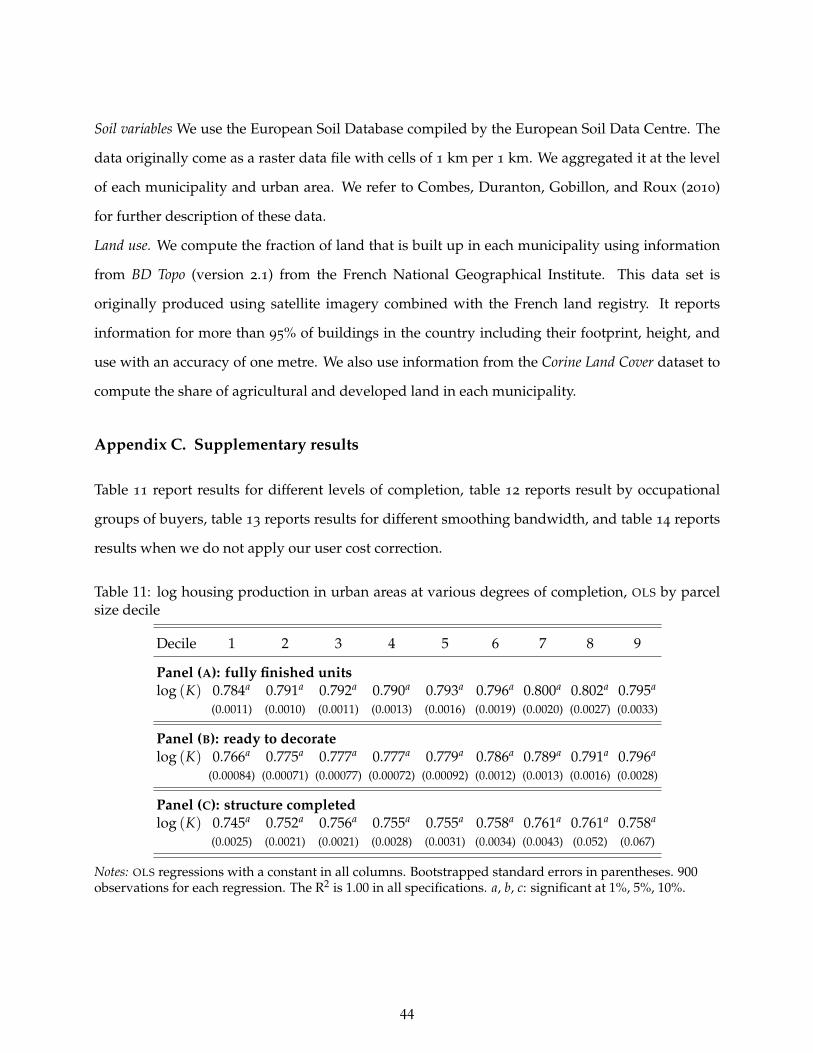
Soil variables We use the European Soil Database compiled by the European Soil Data Centre. The

data originally come as a raster data file with cells of 1 km per 1 km. We aggregated it at the level

of each municipality and urban area. We refer to Combes, Duranton, Gobillon, and Roux (2010)

for further description of these data.

Land use. We compute the fraction of land that is built up in each municipality using information

from BD Topo (version 2.1) from the French National Geographical Institute. This data set is

originally produced using satellite imagery combined with the French land registry. It reports

information for more than 95% of buildings in the country including their footprint, height, and

use with an accuracy of one metre. We also use information from the Corine Land Cover dataset to

compute the share of agricultural and developed land in each municipality.

Appendix C. Supplementary results

Table 11 report results for different levels of completion, table 12 reports result by occupational

groups of buyers, table 13 reports results for different smoothing bandwidth, and table 14 reports

results when we do not apply our user cost correction.

Table 11: log housing production in urban areas at various degrees of completion, OLS by parcelsize decile

Decile 1 2 3 4 5 6 7 8 9

Panel (A): fully finished unitslog (K) 0.784a 0.791a 0.792a 0.790a 0.793a 0.796a 0.800a 0.802a 0.795a

(0.0011) (0.0010) (0.0011) (0.0013) (0.0016) (0.0019) (0.0020) (0.0027) (0.0033)

Panel (B): ready to decoratelog (K) 0.766a 0.775a 0.777a 0.777a 0.779a 0.786a 0.789a 0.791a 0.796a

(0.00084) (0.00071) (0.00077) (0.00072) (0.00092) (0.0012) (0.0013) (0.0016) (0.0028)

Panel (C): structure completedlog (K) 0.745a 0.752a 0.756a 0.755a 0.755a 0.758a 0.761a 0.761a 0.758a

(0.0025) (0.0021) (0.0021) (0.0028) (0.0031) (0.0034) (0.0043) (0.052) (0.067)

Notes: OLS regressions with a constant in all columns. Bootstrapped standard errors in parentheses. 900observations for each regression. The R2 is 1.00 in all specifications. a, b, c: significant at 1%, 5%, 10%.

44

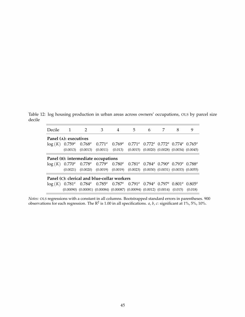
Table 12: log housing production in urban areas across owners’ occupations, OLS by parcel sizedecile

Decile 1 2 3 4 5 6 7 8 9

Panel (A): executiveslog (K) 0.759a 0.768a 0.771a 0.769a 0.771a 0.772a 0.772a 0.774a 0.765a

(0.0013) (0.0013) (0.0011) (0.013) (0.0015) (0.0020) (0.0028) (0.0034) (0.0045)

Panel (B): intermediate occupationslog (K) 0.770a 0.778a 0.779a 0.780a 0.781a 0.784a 0.790a 0.793a 0.788a

(0.0021) (0.0020) (0.0019) (0.0019) (0.0023) (0.0030) (0.0031) (0.0033) (0.0055)

Panel (C): clerical and blue-collar workerslog (K) 0.781a 0.784a 0.785a 0.787a 0.791a 0.794a 0.797a 0.801a 0.805a

(0.00090) (0.00081) (0.00084) (0.00087) (0.00094) (0.0012) (0.0014) (0.015) (0.018)


45

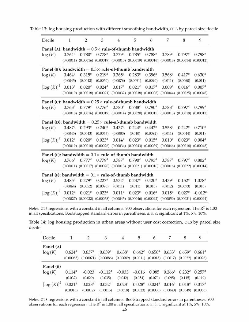
Table 13: log housing production with different smoothing bandwidth, OLS by parcel size decile

Decile 1 2 3 4 5 6 7 8 9

Panel (A): bandwidth = 0.5× rule-of-thumb bandwidthlog (K) 0.764a 0.780a 0.778a 0.779a 0.785a 0.788a 0.789a 0.797a 0.798a

(0.00011) (0.00016) (0.00019) (0.00015) (0.00019) (0.00016) (0.00013) (0.00014) (0.00012)

Panel (B): bandwidth = 0.5× rule-of-thumb bandwidthlog (K) 0.464a 0.315a 0.219a 0.365a 0.283a 0.396a 0.568a 0.417a 0.630a

(0.0045) (0.0042) (0.0050) (0.0076) (0.0091) (0.0090) (0.011) (0.0060) (0.011)

[log (K)]2 0.013a 0.020a 0.024a 0.017a 0.021a 0.017a 0.009a 0.016a 0.007a

(0.00019) (0.00018) (0.00021) (0.00032) (0.00038) (0.00038) (0.00044) (0.00025) (0.00048)

Panel (C): bandwidth = 0.25× rule-of-thumb bandwidthlog (K) 0.763a 0.779a 0.776a 0.780a 0.788a 0.790a 0.788a 0.797a 0.799a

(0.00010) (0.00016) (0.00019) (0.00014) (0.00020) (0.00015) (0.00013) (0.00019) (0.00012)

Panel (D): bandwidth = 0.25× rule-of-thumb bandwidthlog (K) 0.487a 0.293a 0.240a 0.437a 0.244a 0.442a 0.558a 0.242a 0.710a

(0.0045) (0.0043) (0.0063) (0.0080) (0.010) (0.0092) (0.011) (0.0044) (0.011)

[log (K)]2 0.012a 0.020a 0.023a 0.014a 0.023a 0.015a 0.010a 0.023a 0.004a

(0.00019) (0.00018) (0.00026) (0.00034) (0.00043) (0.00039) (0.00046) (0.00018) (0.00048)

Panel (E): bandwidth = 0.1× rule-of-thumb bandwidthlog (K) 0.766a 0.777a 0.779a 0.787a 0.790a 0.793a 0.787a 0.797a 0.802a

(0.00011) (0.00017) (0.00020) (0.00013) (0.00021) (0.00016) (0.00016) (0.00022) (0.00014)

Panel (F): bandwidth = 0.1× rule-of-thumb bandwidthlog (K) 0.485a 0.279a 0.227a 0.532a 0.237a 0.420a 0.439a 0.152a 1.078a

(0.0064) (0.0052) (0.0090) (0.011) (0.011) (0.010) (0.012) (0.0073) (0.010)

[log (K)]2 0.012a 0.021a 0.023a 0.011a 0.023a 0.016a 0.015a 0.027a -0.012a

(0.00027) (0.00022) (0.00038) (0.00045) (0.00046) (0.00042) (0.00050) (0.00031) (0.00044)

Notes: OLS regressions with a constant in all columns. 900 observations for each regression. The R2 is 1.00in all specifications. Bootstrapped standard errors in parentheses. a, b, c: significant at 1%, 5%, 10%.

Table 14: log housing production in urban areas without user cost correction, OLS by parcel sizedecile

Decile 1 2 3 4 5 6 7 8 9

Panel (A)log (K) 0.624a 0.637a 0.639a 0.638a 0.642a 0.650a 0.653a 0.659a 0.661a

(0.00085) (0.00071) (0.00086) (0.00089) (0.0011) (0.0015) (0.0017) (0.0022) (0.0028)

Panel (B)log (K) 0.114a -0.023 -0.112a -0.033 -0.016 0.085 0.266a 0.232a 0.257a

(0.037) (0.029) (0.035) (0.042) (0.054) (0.070) (0.095) (0.115) (0.119)

[log (K)]2 0.021a 0.028a 0.032a 0.028a 0.028a 0.024a 0.016a 0.018a 0.017a

(0.0016) (0.0012) (0.0015) (0.0018) (0.0023) (0.0030) (0.0040) (0.0049) (0.0050)


46

Appendix D. Full identification: constant returns to scales

We now turn to the full identification of the housing production function (up to a constant). Note

first that since builders develop a parcel of a given size at a given location, the land cost entering

their profit maximization program depends only on the location x and parcel area T. We make

the assumption that price of parcels is linear in their size: R = R (x) T, where R is the unit land

price. This is consistent with the intuition that, if parcels are divisible, there should be no arbitrage

possibility between parcels of different sizes.

Builders’ profit at location x is π = P(x)H(K,T)− rK− R (x) T, which is now maximised over

both K and T. Aside from the first-order condition for profit maximisation with respect to capital

(1), there is also one for land:

P (x)∂H (K,T)

∂T= R (x) . (d1)

Plugging the two first-order conditions into the zero-profit condition and simplifying by P(x) leads

to:

H(K,T) = K∂H (K,T)

∂K+ T

∂H (K,T)∂T

. (d2)

This is Euler’s condition that characterises homogeneous functions of degree 1. It implies that

H(K,T) exhibits constant returns to scale.

The first-order condition with respect to K, equation (1), still shows that the housing price can

be rewritten as a function of K and T only, and, as before, the free-entry condition then implies

that it is also the case for the total land price, R (K,T). We can substitute away P (x) from the

free-entry condition by using now the first-order condition for T given by equation (d1). Recalling

that R (x) = R (K,T) /T, this leads to:

∂H (K,T)∂T

=R(x)P(x)

=H (K,T)

rK + R (K,T)R (K,T)

T, (d3)

which is equivalent to:∂ log H (K,T)

∂ log T=

R (K,T)rK + R (K,T)

. (d4)

We obtain an expression that mirrors equation (4) for the elasticity of housing production with

respect to structure. To derive the production function, we substitute expression (5) into (d4) and

obtain:R (K,T)

rK + R (K,T)=

∂ log Z (T)∂ log T

−∫K

r ∂R(K,T)∂T

[rK + R (K,T)]2d log K . (d5)

47

Integrating this equation with respect to log T yields:

log Z (T) = C +∫T

R (K,T)rK + R (K,T)

d log T +∫T

∫K

r ∂R(K,T)∂T

[rK + R (K,T)]2d log Kd log T , (d6)

where C is a constant. Substituting equation (d6) into (5), we get:

log H (K,T) = C +∫T

R (K,T)rK + R (K,T)

d log T +∫K

rKrK + R (K,T)

d log K

+∫T

∫K

r ∂R(K,T)∂T

[rK + R (K,T)]2d log Kd log T (d7)

Note that this expression is consistent with a Cobb-Douglas production function since, for that

function, the two first right-hand side terms are integrals of constant cost shares and collapse into

log T and log K. Moreover, we have R (K,T) = 1−αα r K (where α is the share of capital), which

implies that ∂R(K,T)∂T = 0 and the third right-hand side term of (d7) is then zero.

48

IEB Working Papers

2013

2013/1, Sánchez-Vidal, M.; González-Val, R.; Viladecans-Marsal, E.: "Sequential city growth in the US: does age

matter?"

2013/2, Hortas Rico, M.: "Sprawl, blight and the role of urban containment policies. Evidence from US cities"

2013/3, Lampón, J.F.; Cabanelas-Lorenzo, P-; Lago-Peñas, S.: "Why firms relocate their production overseas?

The answer lies inside: corporate, logistic and technological determinants"

2013/4, Montolio, D.; Planells, S.: "Does tourism boost criminal activity? Evidence from a top touristic country"

2013/5, Garcia-López, M.A.; Holl, A.; Viladecans-Marsal, E.: "Suburbanization and highways: when the Romans,

the Bourbons and the first cars still shape Spanish cities"

2013/6, Bosch, N.; Espasa, M.; Montolio, D.: "Should large Spanish municipalities be financially compensated?

Costs and benefits of being a capital/central municipality"

2013/7, Escardíbul, J.O.; Mora, T.: "Teacher gender and student performance in mathematics. Evidence from

Catalonia"

2013/8, Arqué-Castells, P.; Viladecans-Marsal, E.: "Banking towards development: evidence from the Spanish

banking expansion plan"

2013/9, Asensio, J.; Gómez-Lobo, A.; Matas, A.: "How effective are policies to reduce gasoline consumption?

Evaluating a quasi-natural experiment in Spain"

2013/10, Jofre-Monseny, J.: "The effects of unemployment benefits on migration in lagging regions"

2013/11, Segarra, A.; García-Quevedo, J.; Teruel, M.: "Financial constraints and the failure of innovation

projects"

2013/12, Jerrim, J.; Choi, A.: "The mathematics skills of school children: How does England compare to the high

performing East Asian jurisdictions?"

2013/13, González-Val, R.; Tirado-Fabregat, D.A.; Viladecans-Marsal, E.: "Market potential and city growth:

Spain 1860-1960"

2013/14, Lundqvist, H.: "Is it worth it? On the returns to holding political office"

2013/15, Ahlfeldt, G.M.; Maennig, W.: "Homevoters vs. leasevoters: a spatial analysis of airport effects"

2013/16, Lampón, J.F.; Lago-Peñas, S.: "Factors behind international relocation and changes in production

geography in the European automobile components industry"

2013/17, Guío, J.M.; Choi, A.: "Evolution of the school failure risk during the 2000 decade in Spain: analysis of

Pisa results with a two-level logistic mode"

2013/18, Dahlby, B.; Rodden, J.: "A political economy model of the vertical fiscal gap and vertical fiscal

imbalances in a federation"

2013/19, Acacia, F.; Cubel, M.: "Strategic voting and happiness"

2013/20, Hellerstein, J.K.; Kutzbach, M.J.; Neumark, D.: "Do labor market networks have an important spatial

dimension?"

2013/21, Pellegrino, G.; Savona, M.: "Is money all? Financing versus knowledge and demand constraints to

innovation"

2013/22, Lin, J.: "Regional resilience"

2013/23, Costa-Campi, M.T.; Duch-Brown, N.; García-Quevedo, J.: "R&D drivers and obstacles to innovation in

the energy industry"

2013/24, Huisman, R.; Stradnic, V.; Westgaard, S.: "Renewable energy and electricity prices: indirect empirical

evidence from hydro power"

2013/25, Dargaud, E.; Mantovani, A.; Reggiani, C.: "The fight against cartels: a transatlantic perspective"

2013/26, Lambertini, L.; Mantovani, A.: "Feedback equilibria in a dynamic renewable resource oligopoly: pre-

emption, voracity and exhaustion"

2013/27, Feld, L.P.; Kalb, A.; Moessinger, M.D.; Osterloh, S.: "Sovereign bond market reactions to fiscal rules

and no-bailout clauses – the Swiss experience"

2013/28, Hilber, C.A.L.; Vermeulen, W.: "The impact of supply constraints on house prices in England"

2013/29, Revelli, F.: "Tax limits and local democracy"

2013/30, Wang, R.; Wang, W.: "Dress-up contest: a dark side of fiscal decentralization"

2013/31, Dargaud, E.; Mantovani, A.; Reggiani, C.: "The fight against cartels: a transatlantic perspective"

2013/32, Saarimaa, T.; Tukiainen, J.: "Local representation and strategic voting: evidence from electoral boundary

reforms"

2013/33, Agasisti, T.; Murtinu, S.: "Are we wasting public money? No! The effects of grants on Italian university

students’ performances"

2013/34, Flacher, D.; Harari-Kermadec, H.; Moulin, L.: "Financing higher education: a contributory scheme"

2013/35, Carozzi, F.; Repetto, L.: "Sending the pork home: birth town bias in transfers to Italian municipalities"

2013/36, Coad, A.; Frankish, J.S.; Roberts, R.G.; Storey, D.J.: "New venture survival and growth: Does the fog

lift?"

2013/37, Giulietti, M.; Grossi, L.; Waterson, M.: "Revenues from storage in a competitive electricity market:

Empirical evidence from Great Britain"

IEB Working Papers

2014

2014/1, Montolio, D.; Planells-Struse, S.: "When police patrols matter. The effect of police proximity on citizens’

crime risk perception"

2014/2, Garcia-López, M.A.; Solé-Ollé, A.; Viladecans-Marsal, E.: "Do land use policies follow road

construction?"

2014/3, Piolatto, A.; Rablen, M.D.: "Prospect theory and tax evasion: a reconsideration of the Yitzhaki puzzle"

2014/4, Cuberes, D.; González-Val, R.: "The effect of the Spanish Reconquest on Iberian Cities"

2014/5, Durán-Cabré, J.M.; Esteller-Moré, E.: "Tax professionals' view of the Spanish tax system: efficiency,

equity and tax planning"

2014/6, Cubel, M.; Sanchez-Pages, S.: "Difference-form group contests"

2014/7, Del Rey, E.; Racionero, M.: "Choosing the type of income-contingent loan: risk-sharing versus risk-

pooling"

2014/8, Torregrosa Hetland, S.: "A fiscal revolution? Progressivity in the Spanish tax system, 1960-1990"

2014/9, Piolatto, A.: "Itemised deductions: a device to reduce tax evasion"

2014/10, Costa, M.T.; García-Quevedo, J.; Segarra, A.: "Energy efficiency determinants: an empirical analysis of

Spanish innovative firms"

2014/11, García-Quevedo, J.; Pellegrino, G.; Savona, M.: "Reviving demand-pull perspectives: the effect of

demand uncertainty and stagnancy on R&D strategy"

2014/12, Calero, J.; Escardíbul, J.O.: "Barriers to non-formal professional training in Spain in periods of economic

growth and crisis. An analysis with special attention to the effect of the previous human capital of workers"

2014/13, Cubel, M.; Sanchez-Pages, S.: "Gender differences and stereotypes in the beauty"

2014/14, Piolatto, A.; Schuett, F.: "Media competition and electoral politics"

2014/15, Montolio, D.; Trillas, F.; Trujillo-Baute, E.: "Regulatory environment and firm performance in EU

telecommunications services"

2014/16, Lopez-Rodriguez, J.; Martinez, D.: "Beyond the R&D effects on innovation: the contribution of non-

R&D activities to TFP growth in the EU"

2014/17, González-Val, R.: "Cross-sectional growth in US cities from 1990 to 2000"

2014/18, Vona, F.; Nicolli, F.: "Energy market liberalization and renewable energy policies in OECD countries"

2014/19, Curto-Grau, M.: "Voters’ responsiveness to public employment policies"

2014/20, Duro, J.A.; Teixidó-Figueras, J.; Padilla, E.: "The causal factors of international inequality in co2

emissions per capita: a regression-based inequality decomposition analysis"

2014/21, Fleten, S.E.; Huisman, R.; Kilic, M.; Pennings, E.; Westgaard, S.: "Electricity futures prices: time

varying sensitivity to fundamentals"

2014/22, Afcha, S.; García-Quevedo, J,: "The impact of R&D subsidies on R&D employment composition"

2014/23, Mir-Artigues, P.; del Río, P.: "Combining tariffs, investment subsidies and soft loans in a renewable

electricity deployment policy"

2014/24, Romero-Jordán, D.; del Río, P.; Peñasco, C.: "Household electricity demand in Spanish regions. Public

policy implications"

2014/25, Salinas, P.: "The effect of decentralization on educational outcomes: real autonomy matters!"

2014/26, Solé-Ollé, A.; Sorribas-Navarro, P.: "Does corruption erode trust in government? Evidence from a recent

surge of local scandals in Spain"

2014/27, Costas-Pérez, E.: "Political corruption and voter turnout: mobilization or disaffection?"

2014/28, Cubel, M.; Nuevo-Chiquero, A.; Sanchez-Pages, S.; Vidal-Fernandez, M.: "Do personality traits affect

productivity? Evidence from the LAB"

2014/29, Teresa Costa, M.T.; Trujillo-Baute, E.: "Retail price effects of feed-in tariff regulation"

2014/30, Kilic, M.; Trujillo-Baute, E.: "The stabilizing effect of hydro reservoir levels on intraday power prices

under wind forecast errors"

2014/31, Costa-Campi, M.T.; Duch-Brown, N.: "The diffusion of patented oil and gas technology with

environmental uses: a forward patent citation analysis"

2014/32, Ramos, R.; Sanromá, E.; Simón, H.: "Public-private sector wage differentials by type of contract:

evidence from Spain"

2014/33, Backus, P.; Esteller-Moré, A.: "Is income redistribution a form of insurance, a public good or both?"

2014/34, Huisman, R.; Trujillo-Baute, E.: "Costs of power supply flexibility: the indirect impact of a Spanish

policy change"

2014/35, Jerrim, J.; Choi, A.; Simancas Rodríguez, R.: "Two-sample two-stage least squares (TSTSLS) estimates

of earnings mobility: how consistent are they?"

2014/36, Mantovani, A.; Tarola, O.; Vergari, C.: "Hedonic quality, social norms, and environmental campaigns"

2014/37, Ferraresi, M.; Galmarini, U.; Rizzo, L.: "Local infrastructures and externalities: Does the size matter?"

2014/38, Ferraresi, M.; Rizzo, L.; Zanardi, A.: "Policy outcomes of single and double-ballot elections"

IEB Working Papers

2015

2015/1, Foremny, D.; Freier, R.; Moessinger, M-D.; Yeter, M.: "Overlapping political budget cycles in the

legislative and the executive"

2015/2, Colombo, L.; Galmarini, U.: "Optimality and distortionary lobbying: regulating tobacco consumption"

2015/3, Pellegrino, G.: "Barriers to innovation: Can firm age help lower them?"

2015/4, Hémet, C.: "Diversity and employment prospects: neighbors matter!"

2015/5, Cubel, M.; Sanchez-Pages, S.: "An axiomatization of difference-form contest success functions"

2015/6, Choi, A.; Jerrim, J.: "The use (and misuse) of Pisa in guiding policy reform: the case of Spain"

2015/7, Durán-Cabré, J.M.; Esteller-Moré, A.; Salvadori, L.: "Empirical evidence on tax cooperation between

sub-central administrations"

2015/8, Batalla-Bejerano, J.; Trujillo-Baute, E.: "Analysing the sensitivity of electricity system operational costs

to deviations in supply and demand"

2015/9, Salvadori, L.: "Does tax enforcement counteract the negative effects of terrorism? A case study of the

Basque Country"

2015/10, Montolio, D.; Planells-Struse, S.: "How time shapes crime: the temporal impacts of football matches on

crime"

2015/11, Piolatto, A.: "Online booking and information: competition and welfare consequences of review

aggregators"

2015/12, Boffa, F.; Pingali, V.; Sala, F.: "Strategic investment in merchant transmission: the impact of capacity

utilization rules"

2015/13, Slemrod, J.: "Tax administration and tax systems"

2015/14, Arqué-Castells, P.; Cartaxo, R.M.; García-Quevedo, J.; Mira Godinho, M.: "How inventor royalty

shares affect patenting and income in Portugal and Spain"

2015/15, Montolio, D.; Planells-Struse, S.: "Measuring the negative externalities of a private leisure activity:

hooligans and pickpockets around the stadium"

2015/16, Batalla-Bejerano, J.; Costa-Campi, M.T.; Trujillo-Baute, E.: "Unexpected consequences of

liberalisation: metering, losses, load profiles and cost settlement in Spain’s electricity system"

2015/17, Batalla-Bejerano, J.; Trujillo-Baute, E.: "Impacts of intermittent renewable generation on electricity

system costs"

2015/18, Costa-Campi, M.T.; Paniagua, J.; Trujillo-Baute, E.: "Are energy market integrations a green light for

FDI?"

2015/19, Jofre-Monseny, J.; Sánchez-Vidal, M.; Viladecans-Marsal, E.: "Big plant closures and agglomeration

economies"

2015/20, Garcia-López, M.A.; Hémet, C.; Viladecans-Marsal, E.: "How does transportation shape

intrametropolitan growth? An answer from the regional express rail"

2015/21, Esteller-Moré, A.; Galmarini, U.; Rizzo, L.: "Fiscal equalization under political pressures"

2015/22, Escardíbul, J.O.; Afcha, S.: "Determinants of doctorate holders’ job satisfaction. An analysis by

employment sector and type of satisfaction in Spain"

2015/23, Aidt, T.; Asatryan, Z.; Badalyan, L.; Heinemann, F.: "Vote buying or (political) business (cycles) as

usual?"

2015/24, Albæk, K.: "A test of the ‘lose it or use it’ hypothesis in labour markets around the world"

2015/25, Angelucci, C.; Russo, A.: "Petty corruption and citizen feedback"

2015/26, Moriconi, S.; Picard, P.M.; Zanaj, S.: "Commodity taxation and regulatory competition"

2015/27, Brekke, K.R.; Garcia Pires, A.J.; Schindler, D.; Schjelderup, G.: "Capital taxation and imperfect

competition: ACE vs. CBIT"

2015/28, Redonda, A.: "Market structure, the functional form of demand and the sensitivity of the vertical reaction

function"

2015/29, Ramos, R.; Sanromá, E.; Simón, H.: "An analysis of wage differentials between full-and part-time

workers in Spain"

2015/30, Garcia-López, M.A.; Pasidis, I.; Viladecans-Marsal, E.: "Express delivery to the suburbs the effects of

transportation in Europe’s heterogeneous cities"

2015/31, Torregrosa, S.: "Bypassing progressive taxation: fraud and base erosion in the Spanish income tax (1970-

2001)"

2015/32, Choi, H.; Choi, A.: "When one door closes: the impact of the hagwon curfew on the consumption of

private tutoring in the republic of Korea"

2015/33, Escardíbul, J.O.; Helmy, N.: "Decentralisation and school autonomy impact on the quality of education:

the case of two MENA countries"

2015/34, González-Val, R.; Marcén, M.: "Divorce and the business cycle: a cross-country analysis"

IEB Working Papers

2015/35, Calero, J.; Choi, A.: "The distribution of skills among the European adult population and unemployment: a

comparative approach"

2015/36, Mediavilla, M.; Zancajo, A.: "Is there real freedom of school choice? An analysis from Chile"

2015/37, Daniele, G.: "Strike one to educate one hundred: organized crime, political selection and politicians’

ability"

2015/38, González-Val, R.; Marcén, M.: "Regional unemployment, marriage, and divorce"

2015/39, Foremny, D.; Jofre-Monseny, J.; Solé-Ollé, A.: "‘Hold that ghost’: using notches to identify manipulation

of population-based grants"

2015/40, Mancebón, M.J.; Ximénez-de-Embún, D.P.; Mediavilla, M.; Gómez-Sancho, J.M.: "Does educational

management model matter? New evidence for Spain by a quasiexperimental approach"

2015/41, Daniele, G.; Geys, B.: "Exposing politicians’ ties to criminal organizations: the effects of local government

dissolutions on electoral outcomes in Southern Italian municipalities"

2015/42, Ooghe, E.: "Wage policies, employment, and redistributive efficiency"

2016

2016/1, Galletta, S.: "Law enforcement, municipal budgets and spillover effects: evidence from a quasi-experiment

in Italy"

2016/2, Flatley, L.; Giulietti, M.; Grossi, L.; Trujillo-Baute, E.; Waterson, M.: "Analysing the potential

economic value of energy storage"

2016/3, Calero, J.; Murillo Huertas, I.P.; Raymond Bara, J.L.: "Education, age and skills: an analysis using the

PIAAC survey"

2016/4, Costa-Campi, M.T.; Daví-Arderius, D.; Trujillo-Baute, E.: "The economic impact of electricity losses"

2016/5, Falck, O.; Heimisch, A.; Wiederhold, S.: "Returns to ICT skills"

2016/6, Halmenschlager, C.; Mantovani, A.: "On the private and social desirability of mixed bundling in

complementary markets with cost savings"

2016/7, Choi, A.; Gil, M.; Mediavilla, M.; Valbuena, J.: "Double toil and trouble: grade retention and academic

performance"

2016/8, González-Val, R.: "Historical urban growth in Europe (1300–1800)"

2016/9, Guio, J.; Choi, A.; Escardíbul, J.O.: "Labor markets, academic performance and the risk of school dropout:

evidence for Spain"

2016/10, Bianchini, S.; Pellegrino, G.; Tamagni, F.: "Innovation strategies and firm growth"

2016/11, Jofre-Monseny, J.; Silva, J.I.; Vázquez-Grenno, J.: "Local labor market effects of public employment"

2016/12, Sanchez-Vidal, M.: "Small shops for sale! The effects of big-box openings on grocery stores"

2016/13, Costa-Campi, M.T.; García-Quevedo, J.; Martínez-Ros, E.: "What are the determinants of investment

in environmental R&D?"

2016/14, García-López, M.A; Hémet, C.; Viladecans-Marsal, E.: "Next train to the polycentric city: The effect of

railroads on subcenter formation"

2016/15, Matas, A.; Raymond, J.L.; Dominguez, A.: "Changes in fuel economy: An analysis of the Spanish car

market"

2016/16, Leme, A.; Escardíbul, J.O.: "The effect of a specialized versus a general upper secondary school

curriculum on students’ performance and inequality. A difference-in-differences cross country comparison"

2016/17, Scandurra, R.I.; Calero, J.: “Modelling adult skills in OECD countries”

2016/18, Fernández-Gutiérrez, M.; Calero, J.: “Leisure and education: insights from a time-use analysis”

2016/19, Del Rio, P.; Mir-Artigues, P.; Trujillo-Baute, E.: “Analysing the impact of renewable energy regulation

on retail electricity prices”

2016/20, Taltavull de la Paz, P.; Juárez, F.; Monllor, P.: “Fuel Poverty: Evidence from housing perspective”

2016/21, Ferraresi, M.; Galmarini, U.; Rizzo, L.; Zanardi, A.: “Switch towards tax centralization in Italy: A wake

up for the local political budget cycle”

2016/22, Ferraresi, M.; Migali, G.; Nordi, F.; Rizzo, L.: “Spatial interaction in local expenditures among Italian

municipalities: evidence from Italy 2001-2011”

2016/23, Daví-Arderius, D.; Sanin, M.E.; Trujillo-Baute, E.: “CO2 content of electricity losses”

2016/24, Arqué-Castells, P.; Viladecans-Marsal, E.: “Banking the unbanked: Evidence from the Spanish banking

expansion plan“

2016/25 Choi, Á.; Gil, M.; Mediavilla, M.; Valbuena, J.: “The evolution of educational inequalities in Spain:

Dynamic evidence from repeated cross-sections”

2016/26, Brutti, Z.: “Cities drifting apart: Heterogeneous outcomes of decentralizing public education”

2016/27, Backus, P.; Cubel, M.; Guid, M.; Sánchez-Pages, S.; Lopez Manas, E.: “Gender, competition and

performance: evidence from real tournaments”

2016/28, Costa-Campi, M.T.; Duch-Brown, N.; García-Quevedo, J.: “Innovation strategies of energy firms”

2016/29, Daniele, G.; Dipoppa, G.: “Mafia, elections and violence against politicians”

IEB Working Papers

2016/30, Di Cosmo, V.; Malaguzzi Valeri, L.: “Wind, storage, interconnection and the cost of electricity”

2017

2017/1, González Pampillón, N.; Jofre-Monseny, J.; Viladecans-Marsal, E.: "Can urban renewal policies reverse

neighborhood ethnic dynamics?”

2017/2, Gómez San Román, T.: "Integration of DERs on power systems: challenges and opportunities”

2017/3, Bianchini, S.; Pellegrino, G.: "Innovation persistence and employment dynamics”

2017/4, Curto‐Grau, M.; Solé‐Ollé, A.; Sorribas‐Navarro, P.: "Does electoral competition curb party favoritism?”

2017/5, Solé‐Ollé, A.; Viladecans-Marsal, E.: "Housing booms and busts and local fiscal policy”

2017/6, Esteller, A.; Piolatto, A.; Rablen, M.D.: "Taxing high-income earners: Tax avoidance and mobility”

Cities

[email protected]

www.ieb.edu


Pierre-Philippe Combes, Gilles Duranton, Laurent Gobillon ...

Documents