Piecewise closed-loop equilibria in differential games with ...

HAL Id: hal-01449990https://hal.archives-ouvertes.fr/hal-01449990

Submitted on 30 Jan 2017

HAL is a multi-disciplinary open accessarchive for the deposit and dissemination of sci-entific research documents, whether they are pub-lished or not. The documents may come fromteaching and research institutions in France orabroad, or from public or private research centers.

L’archive ouverte pluridisciplinaire HAL, estdestinée au dépôt et à la diffusion de documentsscientifiques de niveau recherche, publiés ou non,émanant des établissements d’enseignement et derecherche français ou étrangers, des laboratoirespublics ou privés.

Piecewise closed-loop equilibria in differential gameswith regime switching strategies

Ngo Van Long, Fabien Prieur, Mabel Tidball, Klarizze Puzon

To cite this version:Ngo Van Long, Fabien Prieur, Mabel Tidball, Klarizze Puzon. Piecewise closed-loop equilibria indifferential games with regime switching strategies. Journal of Economic Dynamics and Control,Elsevier, 2017, 76, pp.264-284. 10.1016/j.jedc.2017.01.008. hal-01449990

https://hal.archives-ouvertes.fr/hal-01449990

https://hal.archives-ouvertes.fr

Ver

sion

pos

tprin

t

Comment citer ce document :Long, N. V., Prieur, F., Tidball, M., Puzon, K. (2017). Piecewise closed-loop equilibria in

differential games with regime switching strategies. Journal of Economic Dynamics and Control, àparaître, à paraître. DOI : 10.1016/j.jedc.2017.01.008

Accepted Manuscript

Piecewise closed-loop equilibria in differential games with regimeswitching strategies

Ngo Van Long, Fabien Prieur, Mabel Tidball, Klarizze Puzon

PII: S0165-1889(17)30016-7DOI: 10.1016/j.jedc.2017.01.008Reference: DYNCON 3391

To appear in: Journal of Economic Dynamics and Control

Received date: 17 September 2015Revised date: 11 January 2017Accepted date: 14 January 2017

Please cite this article as: Ngo Van Long, Fabien Prieur, Mabel Tidball, Klarizze Puzon, Piecewiseclosed-loop equilibria in differential games with regime switching strategies, Journal of Economic Dy-namics and Control (2017), doi: 10.1016/j.jedc.2017.01.008

This is a PDF file of an unedited manuscript that has been accepted for publication. As a serviceto our customers we are providing this early version of the manuscript. The manuscript will undergocopyediting, typesetting, and review of the resulting proof before it is published in its final form. Pleasenote that during the production process errors may be discovered which could affect the content, andall legal disclaimers that apply to the journal pertain.

http://dx.doi.org/10.1016/j.jedc.2017.01.008

http://dx.doi.org/10.1016/j.jedc.2017.01.008

Ver

sion

pos

tprin

t



ACCEPTED MANUSCRIPT

ACCEPTED MANUSCRIP

T

Piecewise closed-loop equilibria indifferential games with regime switchingstrategies∗

Ngo Van Long†, Fabien Prieur‡, Mabel Tidball,§ and Klarizze Puzon¶

Abstract

We propose a new methodology exploring piecewise closed-loop equilibrium strategies in dif-ferential games with regime switching actions. We develop a general game with two players.Players choose an action that influences the evolution of a state variable, and decide on theswitching time from one regime to another. Compared to the optimal control problem withregime switching, necessary optimality conditions are modified for the first player to switch.When choosing her optimal switching strategy, this player considers the impact of her choiceon the other player’s actions and consequently on her own payoffs. In order to determinethe equilibrium timing of regime changes, we derive conditions that help eliminate candidateequilibrium strategies that do not survive deviations in switching strategies. We then applythis new methodology to an exhaustible resource extraction game.

Key words: differential games; regime switching strategies; technology adoption; non-renewableresources

JEL classification: C61, C73, Q32.

∗We thank Raouf Boucekkine, Larry Karp, Santanu Roy, Amos Zemel and participants in confer-ences and seminars in Annecy, Baton Rouge, Lisbon, Los Angeles and Toulouse. We are also gratefulto the Editor, Herbert Dawid, and three anonymous referees for their valuables comments.†Department of Economics, McGill University, 855 Sherbrooke Street West, Montreal, QC H3A

2T7, Canada. E-mail: [email protected]‡UMR EconomiX, University Paris Nanterre, 94000 Nanterre, France. E-mail:

[email protected]§INRA-LAMETA, 2 place Viala 34060 Montpellier, France E-mail: [email protected]¶LAMETA, University of Montpellier. E-mail: [email protected]

1

Ver

sion

pos

tprin

t



ACCEPTED MANUSCRIPT

ACCEPTED MANUSCRIP

T

1 Introduction 2

1 Introduction

Several decision making problems in economics concern the timing of switching betweenalternative and consecutive regimes. Regimes may refer to technological and/or insti-tutional states of the world. For instance, a firm with an initial level of technology mayfind it optimal to either adopt a new technology or to stick with the old one (Boucekkineet al. 2004). Another example is the decision to phase out existing capital controls ina given economy (Makris, 2001). In all non-trivial problems, switching regime is a de-cision that involves a trade-off, since adopting a new regime brings with it immediatecosts as well as potential future benefits.

There exists a rich literature that deals with endogenous regime shifts modeled asrandom, for instance poisson-type, processes (see van der Ploeg and de Zeeuw, 2014,and Zemel, 2015, for recent applications to climate change economics). The maindifference with this literature is that inducing a regime change is an additional choicevariable in the hands of the decision maker; not a risky event one has to cope with.Another distinction is worth doing between two cases: the one where a regime shiftis caused by one’s rival (e.g., the rival makes a lumpy investment, such as adoptinga new harvesting technology), and the one where it is induced by nature itself (e.g.,when the carbon stock exceeds a critical threshold level). The focus of our paper ison the former case. The latter case (a natural threshold level) has been investigatedby Tahvonen and Withagen (1996), in deterministic setting, and Lemoine and Traeger(2014), in a stochastic environment where the policy maker learns about the thresholdlevel by observing the system response in each period.

In this article, we depart from this literature as we consider regime switching strate-gies in differential games. The game theoretic literature involving regime switchingchoice is sparse. Early papers on dynamic games of regime change do not involve astock variable. In these models, the only relevant state of the system is the identity ofthe players who have adopted the new technology. An example is Reinganum (1981)’smodel of technological adoption decisions of two ex ante identical firms. She assumedthat firms adopt pre-commitment (open-loop) strategies. That is, it is as if a firm entersa binding commitment on its date of technology switch, knowing the adoption date ofthe other firm. Reinganum’s primary finding is that, with two ex-ante identical firmsusing open-loop strategies, the equilibrium features diffusion: One firm will innovatefirst and the other will innovate at a later date. The first player to switch earns higherprofits. Fudenberg and Tirole (1985) revisited Reinganum’s study by using the concept

Ver

sion

pos

tprin

t



ACCEPTED MANUSCRIPT

ACCEPTED MANUSCRIP

T

1 Introduction 3

of pre-emption equilibrium. Focusing on Markov perfect equilibrium (MPE) as thesolution concept, they noted that the second player to switch may try to preempt itsrival and become the first to adopt. At the preemption equilibrium, the first player toswitch advantage vanishes (see Long, 2010, for a survey of this literature).

A second strand of literature pertains to the strategic interaction of agents in relationto the dynamics of a given stock. For instance, Tornell (1997) presented a model thatexplores the relationship between economic growth and institutional change. Infinitely-lived agents solve a differential game that drives the changes in property-rights regimesfor the economy’s capital stock, e.g. common property versus private property. It wasshown that a potential equilibrium of the game involves multiple switching betweenregimes. However, only the symmetric equilibrium was considered, such that the play-ers always choose to switch at the same instant. Consequently, the question of thetiming between switching times was not addressed. In addition, even though Tornellexplicitly defined the MPE for the class of differential games with regime switching,he does not provide a general modeling of switching strategies. One can also mentionthe related analysis by Boucekkine et al. (2011). They analyzed the trade-off betweenenvironmental quality and economic performance using a simple two-player differentialgame where players may switch to a cleaner but less productive technology. But theypaid attention to the open-loop Nash equilibrium only while our view is that commit-ment requirements are simply too strong to model switching strategies as open-loopstrategies.

Undoubtedly, accounting for the existence of some sort of feedback effect in players’switching strategies operating through the state of the system is a challenging task.In particular, it does not seem straightforward at first glance to extend the standarddefinition of markovian rules (whereby strategies precisely depend on the state of thesystem) to this specific class of discrete decisions. To our knowledge, there seems to beno existing study which formally adresses this issue. This is where the first theoreticalcontribution of this paper lies. We develop a general differential game with two playershaving two kinds of strategies. First, players have to choose at each point in time anaction that influences the evolution of a state variable. Second, they may decide onthe timing of switching between alternative and consecutive regimes that differ both interms of the payoff function and the state equation. Ìn this setting, we define a newequilibrium concept, referred to as the piecewise closed-loop Nash equilibrium (PCNEhereafter), which is the natural adaptation of the MPE when timing decisions are part

Ver

sion

pos

tprin

t



ACCEPTED MANUSCRIPT

ACCEPTED MANUSCRIP

T

1 Introduction 4

of the players’ strategy profile. Formally, this boils down to expressing a player’s timingstrategy as a function of the state of the system, which is described by the regime thatis in current operation, and the level of the stock variable at which the player’s regimeswitching problem starts.

For any possible timing, we characterize the necessary optimality conditions forswitching times, both for interior and corner solutions. One interesting finding is that,compared to the necessary conditions characterizing optimal switching in the standard(one-player) optimal control problem or in game with open-loop information structure,we find that the necessary optimal switching conditions are substantially modified forthe player who finds it optimal to move first. Indeed, when choosing the optimal dateand level of the state variable for switching, this player must take into account that(i) her decision will influence the other player’s equilibrium switching strategy in thesubgame that follows, and (ii) the other player’s switching time will impact on herown welfare. Depending on the particular economic problem at hand, the interactionthrough switching times may provide an incentive to either postpone or expedite regimeswitching. Another important issue is how to determine the equilibrium switchingsequence in the PCNE. We resolve this issue by providing conditions that help eliminatecandidate switching sequences that do not survive deviations in switching strategies.

The second contribution of the paper is the application of this new game theoreticmaterial to study a model of management of an exhaustible resource. To date, thereare only a few papers that have studied the relationship between natural resourceexploitation and the timing of technology adoption. Using a finite horizon two-stageoptimal control problem, Amit (1986) explored the case of a petroleum producer whoconsiders switching from a primary to a secondary recovery process. He observed that atechnological switch occurs if the desired extraction rate is greater than the one that canbe obtained by the natural drive, or when the desired final output is more than whatcan be obtained using the primary process. In a recent paper, Valente (2011) analyzeda two-phase endogenous growth model which concerns a switch from an exhaustibleresource input into a backstop technology. He showed that adoption of new technologyimplies a sudden fall in consumption, but an increase in the growth rate.1

We extend this literature by developing a simple differential game of resource ex-traction with technology adoption. In our setting, two players extract an exhaustible

1 In the same vein, Boucekkine et al. (2013) explored a general control problem with both technolog-ical and ecological regime switches. They applied it to address the issue of optimal resource extractionunder ecological irreversibility, and with the possibility to adopt a backstop technology.

Ver

sion

pos

tprin

t



ACCEPTED MANUSCRIPT

ACCEPTED MANUSCRIP

T

2 The general problem 5

resource for consumption purposes. By incurring a lumpy cost, they can adopt a moreefficient extraction technology. So not only do players choose their extractions rates,they also decide whether to adopt the new technology and when. In the application,we first explicitly characterize strategies at the PCNE where both players switch to thenew technology in finite time. We especially focus on the specific economic trade-offsrelated to the new type of regime switching strategies. Then, we investigate the impactof these strategies on both the extraction rates and the timing of adoption of new tech-nologies. Particular emphasis is on the effect of closed-loop strategic interaction on thefirst player to switch’s strategy (as compared to the single-agent case). We show thatsince adoption of the second player to switch is costly for the first player, the latterstrategically chooses his date of adoption so that he induces the former to postpone heradoption. Finally, we deal with the issue of what timing should ultimately arise at theequilibrium by putting forward some conditions under which none of the players havean incentive to deviate from a specified timing.

The paper is organized as follows. Section 2 presents the details of the generalsetup. Section 3 deals with the theory and characterizes optimality conditions specificto regime switching strategies. In Section 4, we study the resource extraction game toillustrate how our methodology works in a simple application. Section 5 is devoted toa discussion of a numerical example and also reviews other potentially interesting andmore involved economic applications of our theory. Finally Section 6 concludes.

2 The general problem

We consider a two-player differential game in which the instantaneous payoff of eachplayer and the differential equation describing the stock dynamics depend on whatregime the system is in. There are a finite number of regimes, indexed by s, and weassume that under certain conditions, the players are able to take action (at some cost)to affect a change of regime. Let S be the set of regimes. For simplicity, we assume thateach player can make a regime switch only once.2 This implies that regime changesare irreversible, i.e., switching back is not allowed. In this case, there are four possibleregimes and the set S is simply: S ≡ 11, 12, 21, 22.

We assume that the system is initially in regime 11. Player 1 can take a “regime2 The assumption is made for convenience. It would be easy to generalize the analysis to situations

where the players can choose any (finite) number of switching dates by emulating Makris (2001)’sapproach (who considers control problems with many switching times) and combining it with ours.

Ver

sion

pos

tprin

t



ACCEPTED MANUSCRIPT

ACCEPTED MANUSCRIP

T


switching action” to switch the system from regime 11 to regime 21, if the other playerhas not made a switch. The first number in any regime index indicates player 1’s moves.The second refers to player 2. Once the system is in regime 21, only player 2 can take aregime switching action, and this leads the system to regime 22. From regime 11, player2 can switch to regime 12 (if player 1 has not made a switch). From regime 12, onlyplayer 1 can make a regime change, and this switches the system to regime 22. If thesystem is in regime 11 and both players take regime change action simultaneously, theregime will be switched to 22. Finally, the system may remain in 11 forever if neitheragent takes a regime change action. Let Si be the subset of S in which player i canmake a regime change. Then S1 = 11, 12 and S2 = 11, 21.

The state variable x is a continuous function for all t and could be in any spaceRm

+ , 1 ≤ m ≤ M . At each instant, each player chooses an action ui, with ui ∈ Rni ,1 ≤ ni ≤ Ni < ∞, that affects the evolution of x. To simplify the exposition, we setm = 1 and ni = n for i = 1, 2. The instantaneous payoff to player i at time t when thesystem is in regime s is

F si (ui(t), u−i(t), x(t)).

If player i takes a regime change action at time ti ∈ R+, a lumpy cost Ωi(ti, x(ti)) isincurred. Then, if for example 0 < t1 < t2 <∞, player 1’s total payoff is

ˆ t1

0

F 111 (u1, u2, x)e−ρtdt+

ˆ t2

t1

F 211 (u1, u2, x)e−ρtdt

+

ˆ ∞

t2

F 221 (u1, u2, x)e−ρtdt− Ω1(t1, x(t1)),

with ρ the discount rate. The differential equation describing the evolution of the statevariable x in regime s is

x = f s(u1, u2, x).

Let us now explain what is meant by the expression “strategy profile” in this settingin which each player has two types of controls. The set of controls is given by Ci =

ui, ti. A strategy consists of an action policy, describing the actions undertaken byeach player at every possible state of the system, (x, s) ∈ R+ × S, and a switching rulethat represents the decision to switch for some relevant level of the state variable. Again,for the sake of exposure, we restrict attention to those strategies that are not time-dependent. This requires that the function Ωi(ti, x(ti)) takes the form e−ρtiωi(x(ti)).

Player i’s action policy is a mapping Φi from the state space R+ ×S to the set Rn.

Ver

sion

pos

tprin

t



ACCEPTED MANUSCRIPT

ACCEPTED MANUSCRIP

T


This is the standard definition of feedback rules for continuous controls. This definitionis not directly transposable to switching strategies, which correspond to a specific typeof discrete controls. However, if one wants to introduce a link between these strategiesand the state of the system, then it is possible to proceed as follows.

Suppose player 1 thinks that if player 2 finds herself in regime 21 at date t, withx(t) (which implies that he switched at an earlier date t1 ≤ t), she will make a switchat a date t2 ≥ t. Then player 1 should think that the interval of time between hisown switching date t1 and the switching date t2 is a function not of any level of thestock, but of the value of the stock at which player 1’s regime change takes place, i.e.,at x(t1) = x1. More generally, we can define the timing strategy of player i, giventhat s ∈ Si, as a mapping θi from R+ × S to R+ ∪ ∞. For instance, from the state(x1, 21), θ2(x1, 21) is the length of time that must elapse before player 2 takes her regimeswitching action, i.e, the duration of regime 21. If θ2(x1, 21) = ∞, then it means thatshe does not want to switch at all from regime 21.

One may note that the θis are not markovian in the usual sense as they are notdefined over any possible level of the stock variable. Indeed, modeling timing decisionsas standard feedback strategies is problematic. It implies that the time to go beforethe next switch of player i is a function of the stock x(t): θi(x(t), s), for all t ≥ t−i = 0

(t−i is either the initial time or the switching time of the other player). Assume thatthe regime switch finally occurs at ti and for a level xi. In order to determine θi, oneneeds to know the evolution of x on the interval [t, ti]. But this depends on the actionpolicies, Φi, of both players, and in particular on that of player −i, which is obviouslynot controlled by player i. This in turn means that x cannot be part of player i’sswitching strategy as otherwise it wouldn’t be robust to deviations. Put differently, wewould then face the problem that the rule itself, i.e., the function θi, changes as a resultof a deviation in Φ−i during some interval of time in between t and ti.3

Switching strategies nevertheless feature a dependence on a specific value of thestock, the one at which each player’s switching problem begins, and for this reason, theycan be labelled as piecewise closed-loop strategies. The corresponding new equilibriumconcept we then introduce is referred to as the piecewise closed-loop (Nash) equilibrium(see e.g., Davis, 1993, and Haurie and Moresino, 2001, for related works). The keypoint is that such a formulation allows us to account for a new kind of feedback effect inplayers’ switching strategies channeling through the state of the system. Our approach

3 This is not the same thing as saying that the decision can be revised in response to changes in thestock variable, induced by a deviation.

Ver

sion

pos

tprin

t



ACCEPTED MANUSCRIPT

ACCEPTED MANUSCRIP

T


obviously differs from what one would obtain with an open-loop information structurewhereby each player chooses her switching time taking the one of the other as given.This leads to the following definition.

Definition 1. • A strategy vector of player i (as guessed by player −i) is a pairψi ≡ (Φi, θi), i = 1, 2.

• A strategy profile is a pair of strategy vectors, (ψ1, ψ2).

• A strategy profile (ψ∗1, ψ∗2) is called a piecewise closed-loop (Nash) equilib-

rium (PCNE), if given that player i uses the strategy vector ψ∗i , the payoff ofplayer j, starting from any state (x, s) ∈ R+ × S, is maximized by using thestrategy vector ψ∗j , where i, j = 1, 2.

In order to determine a PCNE of this game, a natural way to proceed, for anyparticular timing, is to solve (i) the problem corresponding to each subgame in theaction policies, taking as given the switching times (t1, t2),4 and (ii) the switchingproblem of each player in the switching rules, for a particular profile of action strategies(Φ1,Φ2). For that purpose, we shall extend the methodology originally developed byTomiyama (1985) and Amit (1986) to solve finite horizon two-stage optimal controlproblems (for infinite horizon problems, see Makris, 2001). In order to apply thismethodology, we need to impose:

Assumption 1. The functions F si (.) and f s(.), for any s ∈ S, belong to the class C1.

Moreover, the sub-game obtained by restricting the general problem to any regime ssatisfies the Arrow-Kurz sufficiency conditions.

This assumption ensures that our problem is well-behaved and we manipulate smoothenough functions.

Before going to the theoretical analysis, we would like to emphasize that the topicof the paper is all about regime switching strategies in differential games. This meansthat the core of the analysis is entirely devoted to a presentation of the optimalityconditions associated with these strategies and a discussion on the impact of this newsource of interaction on players’ behaviors. We thus abstract from other issues thattypically arise in differential games, like existence and uniqueness of the equilibrium

4 As illustrated by the decomposition above, if the equilibrium timing is such that 0 5 t1 5 t2 5∞,then there are three sub-games to be considered, each being associated with a particular regime.Indeed, for the timing considered, the sequence of regimes is: 11, 21 and 22.

Ver

sion

pos

tprin

t



ACCEPTED MANUSCRIPT

ACCEPTED MANUSCRIP

T

3 Optimality conditions for switching strategies 9

by assuming that a solution exists and focusing on the novel part of the problem.5

The next section presents the set of necessary optimality conditions that characterizea PCNE of the differential game with regime switching strategies.

3 Optimality conditions for switching strategies

The analysis is conducted for a particular timing: 0 5 t1 5 t2 5 ∞. Necessaryoptimality conditions for the other general timing, 0 5 t2 5 t1 5 ∞, can easily bederived by symmetry. First, we state and interpret optimality conditions for an interiorsolution (a solution with ti positive and finite and t1 6= t2), which allows us to highlightthe impact of the interaction through switching strategies on the solution. Next, wewant to know whether a player has an incentive to deviate from the timing considered.For that purpose, corner solutions are carefully studied.

3.1 Interior solution

Assume that there exists a solution (u∗1(t), u∗2(t), x∗(t)) to the differential game definedabove and for given (t1, t2). In any regime s, Player i’s present value Hamiltonian, Hs

i =

F si (ui,Φ−i(x, s), x)e−ρt + λsif

s(ui,Φ−i(x, s), x) with λsi the co-state variable, evaluatedat this solution is denoted by Hs∗

i and we refer to θ′2 as the derivative w.r.t the statevariable x. Our first theorem states the necessary optimality conditions related to theswitching strategies at the interior solution, if it exists. All the proofs are displayed inthe Appendix A.1.

Theorem 1. The necessary optimality conditions for the existence of a PCNE featuringthe timing 0 < t1 < t2 <∞ are:• For player 2:

H21∗2 (t2)− ∂Ω2(t2, x

∗(t2))

∂t2= H22∗

2 (t2) (1a)

λ212 (t2) +

∂Ω2(t2, x∗(t2))

∂x2

= λ222 (t2). (1b)

5 In the literature on differential games, general theorems on existence are not available, except forlinear quadratic games (e.g., Haurie et al., 2012), or some specific class of stochastic capital accumu-lation games (e.g. Dutta and Sundaram, 1993, and Amir, 1996). Even for linear quadratic games,uniqueness cannot be guaranteed. See Dockner et al. (1996) for examples of non-uniqueness.

Ver

sion

pos

tprin

t



ACCEPTED MANUSCRIPT

ACCEPTED MANUSCRIP

T


• For player 1:

H11∗1 (t1)− ∂Ω1(t1, x

∗(t1))

∂t1= H21∗

1 (t1)− [H21∗1 (t2)−H22∗

1 (t2)], (2a)

λ111 (t1) +

∂Ω1(t1, x∗(t1))

∂x1

= λ211 (t1) + θ′2(x∗(t1), 21)[H21∗

1 (t2)−H22∗1 (t2)], . (2b)

To understand these switching conditions for an interior solution, let us focus onthe difference between the optimality conditions of the first player to switch (player 1)and the second (player 2) for the particular timing considered. Player 2’s conditions(1) are similar to the ones derived in multi-stage optimal control literature. Condition(1a) states that it is optimal to switch from the penultimate to the final regime whenthe marginal gain of delaying the switch, given by the difference H21∗

2 (.) − H22∗2 (.),

is equal to the marginal cost of switching, ∂Ω2(t2,x∗(t2))∂t2

. Condition (1b) equalizes themarginal benefit from an extra unit of the state variable x(t2) with the correspondingmarginal cost. It basically says that the value of the co-state, when approached fromthe intermediate regime, plus the incremental switching cost must just equal the valueof the co-state, approached from the final regime. Hence, as long as a player finds itoptimal to be the second player to switch, her optimality conditions are similar to thestandard switching conditions of an optimal control problem.

The novel part of Theorem 1 stems from the problem faced by the player who optsto switch first. Indeed, player 1’s optimality conditions are modified (compared to thesingle agent framework). The first condition (2a) implies that player 1 cares aboutchanges in his situation induced by the switch of player 2. Player 1 decides on hisoptimal switching time by equalizing the marginal gain of delaying the switch, which isgiven by the difference H11∗

1 (.)−H21∗1 (.) to the marginal switching cost, ∂Ω1(t1,x∗(t1))

∂t1−

[H21∗1 (t2) − H22∗

1 (t2)]. The extra-term [H21∗1 (t2) − H22∗

1 (t2)] is the marginal impact ofplayer 2’s switch on player 1. So, player 1 anticipates the impact of player 2’s switch onhis payoff. Depending on the nature of the problem, the additional term can either bepositive or negative. The second optimality condition (2b) is also modified. The costof a marginal increase in x at t1 now includes an extra-term: θ′2(x∗(t1), 21)[H21∗

1 (t2) −H22∗

1 (t2)]. This term reflects the fact that player 1 takes into account his influence onplayer 2’s timing strategy, through the level of the state variable at the switching timex∗(t1). Put differently, player 1 knows that modifying x∗(t1) is a means to delay oraccelerate player 2’s regime switching. In sum, the modified switching conditions ofplayer 1 illustrate the existence of a two-way interaction through switching strategies.

Ver

sion

pos

tprin

t



ACCEPTED MANUSCRIPT

ACCEPTED MANUSCRIP

T


A couple of comments are in order here. First, in (2), the term θ′2(x∗(t1), 21) maylook like a kind of Stackelberg-leadership consideration: Player 1 knows the functionθ∗′2 (x∗(t1), 21), and hence he knows that when he chooses t1 and the level x∗(t1) he isindirectly influencing t2. But this is not really Stackelberg leadership in a global sense.The situation is just like any standard game tree with sequential moves. If a playermoves first, he knows how the second player to switch will move at each subgame thatfollows, and therefore he will take that into account in choosing which subgame he isgoing to induce.

Second, the methodology used here relies extensively on the tools developed bythe multi-stage control theory. Beyond the difference in terms of optimality conditionsdiscussed above, there is another crucial difference between a three-stage optimal controlproblem and our three-stage differential game. Indeed in the former problem, the tworegime switches are triggered by a single agent and each is associated with optimalityconditions similar to (1). Put differently, a single agent would choose two differentswitching instants t1, t2 ∈ (0,∞) and the corresponding optimal values for the statevariable x∗(t1) and x∗(t2). In the game version and for the timing considered here,player 1 – who is supposed to switch first – has no such optimality conditions at player2’ switching time t2. He’s neither the one that has to choose the switching time. Nor,can he optimally adjust the level of the state variable at this instant. Similarly, thereare no optimality conditions for player 2 at t1, the instant when player 1 solves his ownswitching problem (see, for more details, pages 33-36 of the Appendix A.1). However,as mentioned just above, for this particular sequence of moves, player 1 can indirectlyinfluence player 2’s switching decision whereas player 2 cannot.

3.2 Corner solutions

Still for the same timing, we now examine the conditions for one player to choose acorner strategy.

Theorem 2. 1. Suppose player 1 switches at some instant t1 ∈ (0,∞).

• Necessary conditions for player 2 to choose a corner solution with immediateswitching, i.e., t2 = t1 (instead of t2 > t1) are (1b), and

H21∗2 (t2)− ∂Ω2(t2, x

∗(t2))

∂t2≤ H22∗

2 (t2) if t1 = t2 (3)

Ver

sion

pos

tprin

t



ACCEPTED MANUSCRIPT

ACCEPTED MANUSCRIP

T


2. Suppose player 2’s switching problem has an interior solution t2.

• Necessary conditions for player 1 to choose a corner solution with immediateswitching 0 = t1 are (2b), and

H11∗1 (t1)− ∂Ω1(t1, x

∗(t1))

∂t1≤ H21∗

1 (t1)− [H21∗1 (t2)−H22∗

1 (t2)] if 0 = t1 < t2 (4)

• Necessary conditions for player 1 to choose a corner solution of the never switch-ing type t1 = t2 are (2b), and

H11∗1 (t1)− ∂Ω1(t1, x

∗(t1))

∂t1≥ H21∗

1 (t1)− [H21∗1 (t2)−H22∗

1 (t2)] if t1 = t2 (5)

The corner solution t1 = 0 and corresponding necessary conditions have alreadybeen discussed in literature. For t1 = 0, it must be the case that player 1 wants toescape from regime 11 as soon as possible. According to condition (4), this happenswhen a delay in switching yields a marginal gain that is not greater than the marginalloss of foregoing for an instant the benefit of the new regime. Of further interest is theinterpretation of players’ “corner solutions” t1 = t2. Quotes are needed because thosesolutions actually correspond to artificial situations where the timing is (pre)specified(here t1 5 t2). The conditions for them to occur deserve much attention since theyprovide a clear way to check if a candidate equilibrium in switching strategies is robustto deviations. As an illustration, consider player 1’s problem. Conditional on player1 being the first to make a switch and on player 2 being the second, we can derive anecessary condition for t1 to be at the corner t1 = t2. If this condition (5) is satisfied,which means that at t2 a delay in switching yields a marginal gain that is at least ashigh as the marginal loss of foregoing for an instant the benefit of the new regime, thenwe suspect that, when we remove the artificial requirement that t1 5 t2, there will bean incentive for player 1 to choose to make a regime switch in second place. In sucha case, a candidate solution with t1 5 t2 does not survive the incentive for player 1to deviate from it. In other words, condition (5) is necessary for the timing not to berobust to deviations in player 1’s switching strategy. The same reasoning applies toplayer 2’s corner solution t2 = t1.

Of course, the timing is not fixed in our differential game with regime switchingstrategies and the most important task is precisely to determine what will be the timingat the equilibrium, or under which conditions a particular timing will occur. The

Ver

sion

pos

tprin

t



ACCEPTED MANUSCRIPT

ACCEPTED MANUSCRIP

T

4 A resource extraction game with technology adoption 13

analysis of situations where one player may have an incentive to deviate is of crucialimportance to address this non-trivial issue. Indeed, it should allow us to understandwhich timing, between 0 5 t1 < t2 5 ∞ and 0 5 t2 < t1 5 ∞, is consistent with thePCNE requirement.

Let us conclude this section with a brief overview of the other possible combinationsbetween t1 and t2. First, note that there is no counterpart to the necessary conditions(3)-(5) for the corner solution t2 =∞ (see the discussion in Makris, 2001, page 1941).However, the inequality

H21∗2 (t2)− ∂Ω2(t2, x

∗(t2))

∂t2> H22∗

2 (t2) for all t1 ≤ t2 <∞ (6)

is sufficient to establish that player 2 will never find it optimal to switch regime. Next,it is highly unlikely that heterogeneous players decide on the same switching time. So,generically, we do not expect the timing 0 < t1 = t2 <∞ to be a PCNE candidate whenplayers have different costs or preferences. But, it is quite easy to derive the optimalityconditions if that timing is an equilibrium outcome for some non-generic cases.6

The next section is devoted to an application of the theory to an exhaustible resourceproblem. Our purpose is to illustrate how the reasoning above works in a simple examplefrom which we can extract analytical results.

4 A resource extraction game with technology adoption

We consider a differential game of extraction of a non-renewable resource. In the relatedliterature (for extensive surveys on dynamic games in resource economics, refer to Long,2010, 2011), it is generally argued that the presence of rivalry among multiple agentstends to result in inefficient outcomes, e.g. overextraction of natural resources. Anothercommon feature of the frameworks developed in this literature is the assumption thatplayers cannot adopt new technology that will improve their extraction efficiency. It

6 Suppose that it is optimal for the two players to switch at the same date t1 = t2 ∈ (0,∞), for thesame level of the state x∗(t) = x∗(t1) = x∗(t2), then the following conditions must hold, for i = 1, 2:

H11∗i (t)− ∂Ωi(t,x

∗(t))∂ti

= H22∗i (t)

λ11i (t) + ∂Ωi(t,x

∗(t))∂xi

= λ22i (t).

(7)

Finally, conditions corresponding to the cases t1 = t2 = 0 and t1 = t2 =∞ can easily be derived fromthe material presented above.

Ver

sion

pos

tprin

t



ACCEPTED MANUSCRIPT

ACCEPTED MANUSCRIP

T


is usually assumed that consumption is a fixed fraction of the extraction level. In thissection, we relax this assumption and consider the possibility of technological adoptionamong players. That is, players not only choose their consumption, but they also decidewhen to adopt the more efficient extraction technology. This consideration representsanother contribution of this paper.

Our resource extraction game comprises I = 2 players. Let ui(t) denote the con-sumption rate of player i, i = 1, 2, at time t ≥ 0. Meanwhile, let ei(t) be player i’sextraction rate from the resource at time t ≥ 0. Extraction is converted into con-sumption according to the following technology: γiui(t) = ei(t), where γ−1

i is a positivenumber that reflects a player’s degree of efficiency in transforming the extracted naturalresource into a consumption good.

Two production technologies, described only by the parameter γi, are available toplayer i from t = 0. Because players’ technological menus may differ, one needs tointroduce a specific index for the player’s actual technology. It is assumed that player1 starts with technology l = 1 and has to decide: (i) whether he switches to technologyl = 2, and (ii) when. The state of technology of the other player, 2, is labelled as k anda technological regime is represented by s = lk, with l, k = 1, 2. For each player i, theranking between the parameters satisfies: γ1

i > γ2i , which means that the second new

technology is more efficient than the old one. A possible indicator of technological gainfor player i from adoption is the ratio γ2i

γ1i∈ (0, 1), such that the smaller is the ratio, the

higher is the gain.Let x(t) be the stock of the exhaustible resource, with the initial stock x0 given. As

in section 2, t1 and t2 are the switching times. Suppose 0 < t1 < t2, then the evolutionof the stock is given by the following differential equation:

x =

−γ11u1 − γ1

2u2 if t ∈ [0, t1)

−γ21u1 − γ1

2u2 if t ∈ [t1, t2)

−γ21u1 − γ2

2u2 if t ∈ [t2,∞)

At the switching time, if any, player i incurs a cost that is defined in terms of thelevel of the state variable at which the adoption occurs, x(ti) = xi. Let ωi(x(ti)) be thiscost, with ω′i(.) ≥ 0. It takes the form: ωi(xi) = χi + βixi, where χi ≥ 0, βi ≥ 0, andχi is the fixed cost related to technology investment. These may include initial outlayfor machinery, etc. On the other hand, βi represents the sensitivity of adoption cost tothe level of the exhaustible resource at the instant of switch. Our assumption implies

Ver

sion

pos

tprin

t



ACCEPTED MANUSCRIPT

ACCEPTED MANUSCRIP

T


that the cost of adopting new technology is increasing in xi. This assumption conveysthe idea that the lower the level of the (remaining) stock of resource, the lower thecost of adopting the new technology. It could reflect the fact that scientific progress oninstallation of resource-saving technology is continually made as the scarcity becomesmore acute. The direct switching cost is discounted at rate ρ. As seen from the initialperiod, if a switch occurs at ti, the discounted cost amounts to e−ρtiωi(xi) (this is ourΩi(ti, x(ti)) of Section 2). Finally, each player’s gross utility function depends on herconsumption only and takes the logarithmic form: F (ui, u−i, x) = ln(ui).

Hereafter, our aim is to apply the methodology developed in Section 3 to this simpleproblem. We start by explicitly characterizing both extraction and switching strategiesat the PCNE with 0 < t1 < t2 < ∞. Then, in the wake of the discussion followingTheorem 1, we illustrate the impact of strategic interaction on the decision to adopt thenew technology. Finally, we present the conditions under which neither the players wantto deviate from the timing considered, nor they have an incentive to adopt a cornerstrategy. Note that in the subsequent analysis, we pay attention only to the class oflinear feedback strategies for extraction rates.7 Moreover, we shall denote x∗(ti) = x∗i ,the level of the stock of resource at which player i decides to switch at the PCNE andcall it the switching point. All the proofs are relegated in Appendix B.

4.1 PCNE with 0 < t1 < t2 <∞The general game – defined as a sequence of three subgames 11, then 21, and finally22 – is solved backward. Let us put aside the issue of the existence of the PCNE forthe moment (this analysis is postponed to the very end of Section 4.3), and focus onits characteristics assuming that it exists. In the remainder of the analysis, we need todefine the function ζ(x1;x∗2) as follows

ζ(x1;x∗2) = 1− e−ρθ2(x1,21)

2ln(1− ρβ2x

∗2)− β1(Γ(x∗2) + ρx1). (8)

For the problem to be well-defined, hereafter we assume that ζ(x0;x∗2) > 0. In or-der to avoid unnecessary discussion on technical grounds, we also require that x0 <

7 To echo footnote 6, it is well-known that there may exist other feedback, non-linear, equilibriain linear-quadratic games (see Dutta and Sundaram, 1993). If we are aware that different types ofextraction strategies may lead to a different timing at the PCNE, assessing the issue of uniqueness isbeyond the scope of the paper.

Ver

sion

pos

tprin

t



ACCEPTED MANUSCRIPT

ACCEPTED MANUSCRIP

T


min (ρβ1)−1, (ρβ2)−1.8 Then we can establish that:

Proposition 1. The PCNE with 0 < t1 < t2 <∞ has the following features:

• In regime 22: extraction rates are given by

γ21Φ1(x, 22) = γ2

2Φ2(x, 22) = ρx. (9)

• In regime 21: extraction rates are defined by

γ21Φ1(x, 21) = γ1

2Φ2(x, 21) = Γ(x∗2) + ρx with Γ(x∗2) =ρ2β2(x∗2)2

1− β2ρx∗2. (10)

There exists a unique switching point, x∗2, for player 2, that solves

ρω2(x∗2) = ln(1− β2ρx∗2)− ln

(γ2

2

γ12

). (11)

The time-to-go (before switching) strategy is t2 − t1 = θ2(x∗1, 21), with

θ2(x∗1, 21) =1

2ρln

[(1− ρβ2x

∗2)x∗1x∗2

+ ρβ2x∗2

]=

1

2ρln

[Φi(x

∗1, 21)

Φi(x∗2, 21)

]. (12)

• In regime 11: extraction strategies satisfy

γ11Φ1(x, 11) = γ1

2Φ2(x, 11) = Λ(x∗1, x∗2) + ρx,

with Λ(x∗1, x∗2) =

Γ(x∗2)+ρx∗1[1−ζ(x∗1;x∗2)]

ζ(x∗1;x∗2),

The level of the stock for switching x∗1 is uniquely defined by

ρω1(x∗1) = e−ρθ2(x∗1,21) ln (1− ρβ2x∗2) + ln[ζ(x∗1;x∗2)]− ln

(γ2

1

γ11

). (13)

With (x∗1, x∗2) being determined above, the switching time t1 = θ1(x0, 11) is

θ1(x0, 11) =1

2ρln

(Λ(x∗1, x

∗2) + ρx0

Λ(x∗1, x∗2) + ρx∗1

)=

1

2ρln

[Φi(x0, 11)

Φi(x∗1, 11)

].

Let us start with the analysis of extraction strategies. One immediately observesthat, in each regime, the two players have the same extraction rates, but generally

8 These technical conditions are not central in the upcoming economic analysis.

Ver

sion

pos

tprin

t



ACCEPTED MANUSCRIPT

ACCEPTED MANUSCRIP

T


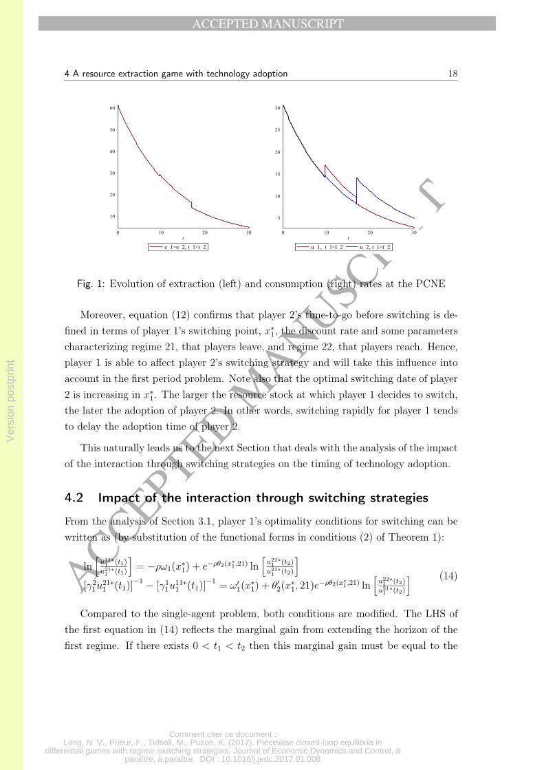
not the same consumption rates. This feature is due to the logarithmic utility. Fromequations (9) and (10), we see that if β2 > 0, then the adoption of the new technology byplayer 2 translates into a downward jump in the extraction rate at time t2. Intuitively,with the new technology, one needs less resource to produce a given amount of theconsumption good. The impact of player 2’s adoption on her own consumption fromtime t2 onward must be positive (for otherwise, she would not make the switch).

Even more interesting is the fact that it is unsure whether the downward adjustmentin extraction also occurs at player 1’s switching date. Indeed, the movement of theextraction rate at t1 depends on whether ζ(x∗1;x∗2) ≶ 1,9 which is unclear in general.This emphasizes the impact of the interaction via switching strategies on extractionstrategies. Player 1 knows that he will be worse off after player 2’s adoption becausehe will bear the decrease in extraction rates while being unable to compensate it bychanging his own technology, as it is fixed after time t1. This may induce him tocompensate this future anticipated costly event by increasing the extraction rate at t1.

As an illustration, we can take a numerical example,10 for which the extraction rateactually increases at the date of adoption of player 1. As depicted in Figure 1, theupward jump in the extraction rate allows player 1 to substantially increase the rate ofconsumption at t1 in the anticipation of future bad times.

As to the switching strategies, the combination of the optimality conditions dis-played in Theorem 1 ((1) for player 2, and (2) for player 1) yields conditions (11) and(13) in the application. According to (11), for instance, player 2 chooses the switch-ing point x∗2 that equalizes the net marginal gain of adoption (RHS) to the (constantvalue) direct marginal switching cost, ρω2(x∗2) (LHS). The gain from adoption is mea-sured in terms of increased consumption rates; it is given by the difference between thedirect marginal gain from adoption, − ln

(γ22γ12

), and the downward adjustment of the

extraction rate, represented by ln(1− ρβ2x∗2) < 0.11

9 This expression provides information on the magnitude and direction of the adjustment of extrac-tion – and player 2’s consumption since she keeps using the same technology – occurring at the instantof the transition from regime 11 to regime 21.

10 We use the following set of parameters: x0 = 1500, β1 = 0.001, β2 = 0.01, χ1 = 1, χ2 = 10,γ1

1 = 2, γ21 = 1.715, γ1

2 = 2, γ22 = 1, ρ = 0.04. For these parameter values, technological gain from

adoption is larger for player 2 than for player 1; but adoption costs are much higher for the former.There exists a unique PCNE, in linear feedback rules for extraction, at which player 1 switches first,then followed by player 2, switching times and points being given by: (t1, x

∗1) = (9.548, 678.332) and

(t2, x∗2) = (16.847, 352.686).

11 This is evaluated in utility terms. The same logic is at work for player 1 except that the adjustmentof the extraction rate at his switching time is given by ln[ζ(x∗1;x

∗2)] and he also has to take into account

the change in extraction at player 2’s adoption time, once discounted appropriately.

Ver

sion

pos

tprin

t



ACCEPTED MANUSCRIPT

ACCEPTED MANUSCRIP

T


Fig. 1: Evolution of extraction (left) and consumption (right) rates at the PCNE

Moreover, equation (12) confirms that player 2’s time-to-go before switching is de-fined in terms of player 1’s switching point, x∗1, the discount rate and some parameterscharacterizing regime 21, that players leave, and regime 22, that players reach. Hence,player 1 is able to affect player 2’s switching strategy and will take this influence intoaccount in the first period problem. Note also that the optimal switching date of player2 is increasing in x∗1. The larger the resource stock at which player 1 decides to switch,the later the adoption of player 2. In other words, switching rapidly for player 1 tendsto delay the adoption time of player 2.

This naturally leads us to the next Section that deals with the analysis of the impactof the interaction through switching strategies on the timing of technology adoption.

4.2 Impact of the interaction through switching strategies

From the analysis of Section 3.1, player 1’s optimality conditions for switching can bewritten as (by substitution of the functional forms in conditions (2) of Theorem 1):

ln[u11∗1 (t1)

u21∗1 (t1)

]= −ρω1(x∗1) + e−ρθ2(x∗1,21) ln

[u22∗1 (t2)

u21∗1 (t2)

]

[γ21u

21∗1 (t1)]

−1 − [γ11u

11∗1 (t1)]

−1= ω′1(x∗1) + θ′2(x∗1, 21)e−ρθ2(x∗1,21) ln

[u22∗1 (t2)

u21∗1 (t2)

] (14)

Compared to the single-agent problem, both conditions are modified. The LHS ofthe first equation in (14) reflects the marginal gain from extending the horizon of thefirst regime. If there exists 0 < t1 < t2 then this marginal gain must be equal to the

Ver

sion

pos

tprin

t



ACCEPTED MANUSCRIPT

ACCEPTED MANUSCRIP

T


marginal cost of switching at t1. Now, the marginal switching cost (RHS) is augmented(in absolute magnitude) by the extra-term e−ρθ2(x∗1,21) ln[

u22∗1 (t2)

u21∗1 (t2)]. Player 1 anticipates

that his switching decision will be followed by the switch (in finite time too) of thesecond player and that player 2’s switch will be costly to him. So, it means that player1’s marginal cost of switching at time t1 is higher than it would be in the absence ofplayer 2. Other things equal (x1 constant), this would imply that the switch shouldoccur at a later date, i.e., player 1, when interacting with player 2, has an incentive topostpone adoption.

The second equation in (14) equalizes the marginal benefit from an extra unit ofthe state variable x1 (LHS) with the corresponding marginal cost (RHS). This cost islower in the game than in the control problem because, from (12), θ′2(x∗1, 21) > 0 and weknow that ln[

u22∗1 (t2)

u21∗1 (t2)] < 0. Indeed, changing x1 marginally yields an additional benefit

here. Other things equal (t1 constant), it allows player 1 to induce player 2 to delaythe instant of her switch. The impact of player 2’s switch will then be felt less acutelybecause of discounting. This in turn implies that player 1’s adoption should occur at ahigher x∗1. This second effect tends to make it worthwhile for player 1 to adopt at anearlier date (because the trajectory of x is monotone non-increasing).

In summary, as a result of the interaction with player 2, player 1 has an incentive todelay the adoption of the new technology (first-order effect corresponding to the firstcondition in (14)). It does not mean, however, that he will not adopt before player2. According to the second condition in (14), the sooner the adoption of player 1, thelower the negative impact of player 2’s adoption on his welfare (second-order effect).

To conclude this analysis, a striking result can be obtained by focusing on thespecial case where ω1(.) ≡ 0: Player 1’s switching cost is identically zero, so that itis independent of the stock of resource. In this case, if there were no game-theoreticconsiderations, we know that the solution of the optimal control problem would bet1 = 0: Player 1 would adopt the new technology instantaneously because it is moreefficient than the old one. Conclusions are very different in our game setting. Itis optimal for player 1 to switch at a strictly positive date t1 because, by delayingadoption, player 1 affects player 2’s decision in such a way that the cost imposed by heradoption is dampened. In the same vein, from the numerical example, we obtain thatif player 1 was the only one allowed to switch technology, then he would adopt at anearlier date than when he has to adapt to player 2’s adoption (t′1 = 0.805 < t1 = 9.548).

Let us now turn to the last part of the application, whose purpose is to examine

Ver

sion

pos

tprin

t



ACCEPTED MANUSCRIPT

ACCEPTED MANUSCRIP

T


the conditions under which the timing under scrutiny is robust to deviations in players’switching strategies, and players do not opt for corner strategies.

4.3 Incentives to deviate from the specified timing

As outlined in Section 3.2, a player may find the timing 0 5 t1 < t2 5∞ non-optimal.For instance, guessing that player 1 will switch at t1(<∞), player 2 may prefer switchingat a date no later than t1, i.e., deviate from the specified timing. As far as non-optimaltiming are concerned, it can be shown that

Proposition 2. Suppose player 1 adopts the new technology at t1. If player 2 wants todeviate from the timing 0 5 t1 < t2 5∞, then it must hold that

ρω2(x∗1) ≤ ln(1− ρβ2x∗1)− ln

(γ2

2

γ12

). (15)

Given that player 2’s adoption takes place at t2, player 1 has an incentive to deviateonly if:

ρω1(x∗2) ≥ ln[ζ(x∗2;x∗2)] + ln(1− ρβ2x∗2)− ln

(γ2

1

γ11

). (16)

For an interpretation, it is enough to consider player 2’s necessary condition, givenby equation (15) and to draw a parallel with the corresponding condition for a interiorsolution (11). The question is when would player 2 find it optimal to skip regime 21and directly go to regime 22, given that player 1 has adopted at date 0 < t1 < ∞?It turns out that what matters to player 2, when she contemplates the opportunity toadopt right after player 1’s adoption, is still the balance between the marginal gain andcost of adoption, now evaluated at player 1’s switching point. So according to (15),player 2 wants to deviate from the timing t1 5 t2 when the net marginal benefit fromswitching (RHS) outweighs the direct marginal switching cost (LHS), as soon as player1 has adopted and for a switching point x∗1.

As mentioned in the discussion following Theorem 2, necessary conditions for thetiming not to be robust to deviations are derived from the analysis of hypothetical cor-ner solutions where the switching time of one player is assumed to be given.12 Butswitching times are not given in the game setting since they are part of players’ strate-gies. In particular, when looking at player 2’s problem, condition (15), whose standard

12 For instance, condition (15) is obtained when considering t2 → t1, for t1 given; this is the limit ofthe optimality condition (11) for x∗2 → x∗1, when one replaces the equality with inequality “≤”.

Ver

sion

pos

tprin

t



ACCEPTED MANUSCRIPT

ACCEPTED MANUSCRIP

T


interpretation in a single-agent framework would be that player 2 is willing to adoptimmediately at t1, actually characterizes the situation where she has an incentive to de-viate from the considered timing, i.e., to adopt before player 1. A symmetric reasoningapplies to player 1.

As the whole analysis has been conducted for the timing 0 5 t1 < t2 5 ∞, onelogically expects that we can set out conditions under which the timing is indeed robustto deviations. This is done by imposing, for i = 1, 2:

ρω2(x∗i ) + ln

(γ2

2

γ12

)> ρω1(x∗i ) + ln

(γ2

1

γ11

), (17a)

ζ(x∗i ;x∗i ) > 1, (17b)

which are sufficient for the opposite of condition (15) and (16) hold. Condition (17a) isespecially intuitive as it requires the first player to adopt be also the one who faces thelowest net adoption cost, ρωi(x∗i )+ln

(γ2iγ1i

), regardless of the switching point considered.

Before ending the analysis, it is worth considering the other situations where thePCNE associated with timing 0 5 t1 < t2 5 ∞ may exhibit a true corner structurewith, for example, player 1 adopting immediately at t1 = 0, or player 2 never adopting(t2 =∞). Our results, that are obtained by applying the conditions (3)-(5) of Theorem2 and (6) to the resource game, can be summarized in the following proposition.

Proposition 3. • Assume that player 1’s switching problem has an interior solu-tion t1. A sufficient condition for player 2 to choose the “never switching strategy,”so that 0 < t1 < t2 =∞, is that

ρω2(0) + ln

(γ2

2

γ12

)≥ 0. (18)

• Assume that player 2’s switching problem has an interior solution t2. A necessarycondition for player 1 to switch immediately at the beginning, so that 0 = t1 <

t2 <∞ is

ρω1(x0) + ln

(γ2

1

γ11

)≤ e−ρθ2(x0,21) ln(1− β2ρx

∗2) + ln[ζ(x0;x∗2)]. (19)

• A combination of immediate and never switching 0 = t1 < t2 =∞ may arise only

Ver

sion

pos

tprin

t



ACCEPTED MANUSCRIPT

ACCEPTED MANUSCRIP

T

5 Discussion 22

if (18) and

ρω1(x0) + ln

(γ2

1

γ11

)≤ 0, (20)

hold.

Conditions for a corner solution also have very simple interpretations. For instance,according to condition (18), player 2 never finds it worthwhile to adopt the new tech-nology if the fixed cost of adoption ρω2(0), weighted by the rate of time preference, islarger than the direct gain from switching even when the resource gets close to exhaus-tion (in our setting, the stock of resource is asymptotically exhausted). In the samevein, for a player to be willing to adopt the new technology immediately it must holdthat the switching cost at the initial resource level is lower than the gain from adoption.In the latter case, the particular tradeoff is influenced by the other player’s switchingdecision to switch in finite time (19) or to keep the old technology forever (20).13

Since we have been interested so far in the analysis of the interior solution, we finallyhave to impose conditions that allow us to disregard corner solutions. This we can doby assuming that

ρω2(0) + ln(γ22γ12

)< 0,

ρω1(x0) + ln(γ21γ11

)> max

0, e−ρθ2(x0,21) ln(1− β2ρx

∗2) + ln[ζ(x0;x∗2)]

.

(21)

The last important thing to note is that conditions (17) and (21) are also sufficient toconclude that the PCNE with 0 < t1 < t2 <∞, discussed in Section 4.1, indeed exists.

5 Discussion

5.1 Further insights from numerical analysis

It is worth assessing the impact of technology adoption in the resource game. Forthat purpose, we can compare the PCNE with 0 < t1 < t2 < ∞ with the benchmarksituation in which none of the players can take a regime change decision. In this case,there also exists a unique PCNE, which mimics the corner solution with t1 = t2 = ∞.

13 There are three cases left: (i) Players might wish to adopt their new technology at the same dateand for the same stock of resource. Or, (ii) they might both prefer switching instantaneously; or (iii)on the contrary they might prefer sticking to the first technology forever. If there is heterogeneity inswitching costs, case (i) cannot be an equilibrium outcome. The conditions for having the two otherpossibilities can easily be derived from Proposition 3 (see the Appendix B.4).

Ver

sion

pos

tprin

t



ACCEPTED MANUSCRIPT

ACCEPTED MANUSCRIP

T

5 Discussion 23

But one should keep in mind that, for the parameter values chosen (see footnote 12),this benchmark cannot arise as an equilibrium outcome in the game with two playershaving a switching decision.

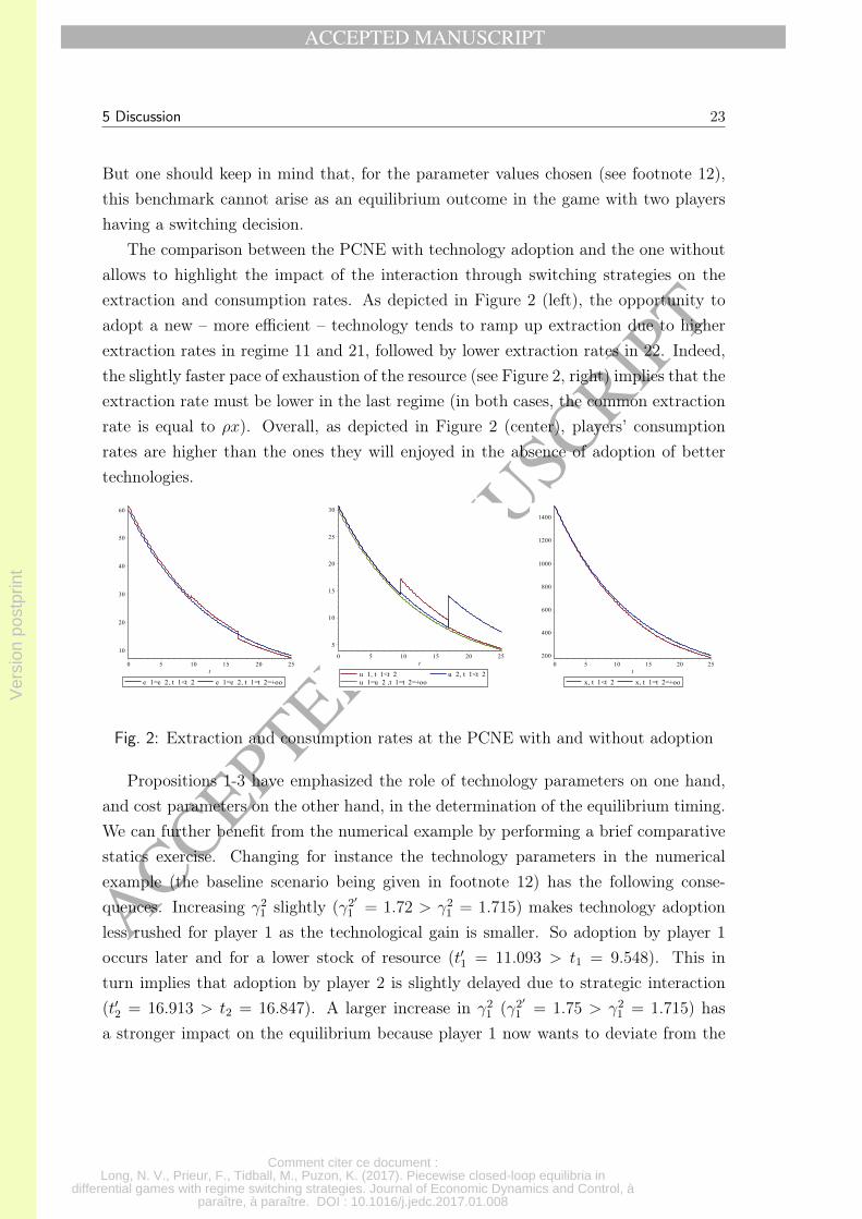
The comparison between the PCNE with technology adoption and the one withoutallows to highlight the impact of the interaction through switching strategies on theextraction and consumption rates. As depicted in Figure 2 (left), the opportunity toadopt a new – more efficient – technology tends to ramp up extraction due to higherextraction rates in regime 11 and 21, followed by lower extraction rates in 22. Indeed,the slightly faster pace of exhaustion of the resource (see Figure 2, right) implies that theextraction rate must be lower in the last regime (in both cases, the common extractionrate is equal to ρx). Overall, as depicted in Figure 2 (center), players’ consumptionrates are higher than the ones they will enjoyed in the absence of adoption of bettertechnologies.

Fig. 2: Extraction and consumption rates at the PCNE with and without adoption

Propositions 1-3 have emphasized the role of technology parameters on one hand,and cost parameters on the other hand, in the determination of the equilibrium timing.We can further benefit from the numerical example by performing a brief comparativestatics exercise. Changing for instance the technology parameters in the numericalexample (the baseline scenario being given in footnote 12) has the following conse-quences. Increasing γ2

1 slightly (γ2′1 = 1.72 > γ2

1 = 1.715) makes technology adoptionless rushed for player 1 as the technological gain is smaller. So adoption by player 1occurs later and for a lower stock of resource (t′1 = 11.093 > t1 = 9.548). This inturn implies that adoption by player 2 is slightly delayed due to strategic interaction(t′2 = 16.913 > t2 = 16.847). A larger increase in γ2

1 (γ2′1 = 1.75 > γ2

1 = 1.715) hasa stronger impact on the equilibrium because player 1 now wants to deviate from the

Ver

sion

pos

tprin

t



ACCEPTED MANUSCRIPT

ACCEPTED MANUSCRIP

T

5 Discussion 24

timing t1 < t2 by switching in second position. On the contrary, a sufficient decrease inγ2

1 (γ2′1 = 1.6 < γ2

1 = 1.715) means that technology adoption is even more worthwhileand gives player 1 the incentive to adopt a corner strategy by choosing t′1 = 0. In thesame vein, a rise in γ2

2 (γ2′2 = 1.2 > γ2

2 = 1), which means that switching technology isless beneficial to player 2, tends to postpone her adoption (t′2 = 29.241 > t2 = 16.847).At the same time, and in accordance with player 2’s adjustment, player 1’s adoptionoccurs earlier and for a higher stock of the resource (t′1 = 1.811 > t1 = 9.548). Anotherinteresting feature is that as player 2’s adoption is now less harmful to player 1 (thedownward jump in extraction is smaller and t2 larger), he no longer has to compensatethis future costly event by increasing the extraction rate at his own date of adoption(see the discussion in Section 4.1). Thus, extraction rates jump down at both switchingtimes. Finally, if player 2’ gain from adoption becomes higher because of a smaller γ2

2

(γ2′2 = 0.8 < γ2

2 = 1), then we obtain that none of the players find the timing optimalanymore. Both want to switch positions and allow player 2 to move first.

5.2 Other potential applications of the methodology

In the present analysis, we have chosen the simplest economic problem on purpose aswe wanted to illustrate how the methodology works in an application. However, ourcontribution can be useful for researchers working in various fields of the economicanalysis. It provides economists with a powerful tool to assess any situation where thedecision maker can take some “discrete” decisions, as opposed to standard continuouscontrols, that affect his/her situation and, since we do not live in an isolated world, thesituation of other decision makers surrounding him/her. This may include much moreinvolved economic problems such as the following ones.14

Our methodology can first be applied to extended versions of recent papers in re-source economics, like Jaakola (2012) (or Gerlagh and Liski, 2011). Jaakola considersthe dynamic and strategic interaction between an oil exporter, who owns an exhaustiblepolluting resource, and an oil importer who invests in R&D to make a backstop technol-ogy cheaper. In this paper, one of the players, the oil importer, has a regime switchingor timing decision as he/she chooses the instant when to switch to the backstop (sothe date of economic exhaustion of the resource).15 In order for this general problem

14 A richer list of relevant applications and more institution-oriented examples can be found inBoucekkine et al. (2013).

15 Note that Jaakola mostly focuses on the open-loop Nash equilibrium while we believe that com-mitment requirements are simply too strong to model switching strategies as open-loop strategies.

Ver

sion

pos

tprin

t



ACCEPTED MANUSCRIPT

ACCEPTED MANUSCRIP

T

5 Discussion 25

to provide an interesting application of our theory, we would have to assign a regimeswitching decision to the other player. It is well-known that a major weakness of oilexporting economies is the lack of economic diversification, which notably makes themvulnerable to the volatilities of prices (Arezki et al., 2011). One option would thenbe to assume that the oil-exporter can also decide, given the threat of a switch to thebackstop by the other player, when to engage in a process of diversification. Still onnatural resources management by oligopolies, another interesting analysis is the oneof the impact of oil discovery on the oligopoly equilibrium (Benchekroun and Long,2006). The problem would consist in defining oil discovery as a timing strategy, playersbeing able to increase theirs stocks at some date ti by paying a lumpy exploration costdefined over the actual stocks of resources of all players. This would also contributeto the literature on the trade-offs between exploration and extraction, which usuallydisentangles those issues by assuming that an oil producer chooses its exploration effortat the initial date and then its extraction path (the problem being solved backward,see Gaudet and Lasserre, 1988, and more recently, Daubanes and Lasserre, 2015).

The second class of applications of our theory has to do with the dynamics ofinstitutions in resource-rich economies. For instance, Boucekkine et al. (2016) analyzethe dynamic and strategic interaction between an autocratic elite and the citizens. Intheir setting, there is an initial regime during which the elite control all the resourcesand take all the decisions. The citizens can only take a regime change decision bychoosing the date of a costly revolution against the elite, which leads the system to amore democratic regime. A natural extension of this work may consist in allowing theelite to have a switching strategy too. In line with this paper, the elite may be ableto revise their redistribution and/or repression policy at some point in time, when thethreat of revolution becomes serious. A related but different topic is the one dealingwith conflicts related to natural resources. Van der Ploeg (2016) develops a differentialgame in which a resource extraction problem is coupled with a contest for the controlof the resource by rival groups. He adopts the traditional way of modeling conflict byusing a contest success function (see Tullock, 1980). His approach basically boils downto disentangling the problem of choosing the fighting efforts – which becomes staticand whose resolution gives the symmetric equilibrium in these efforts at each date –from the problem of choosing extraction rates – which is in essence a dynamic one. Analternative approach would be to assume that rival groups can decide the date when totrigger (at some cost) a conflict against the others to expropriate them or increase theshare of the stock of resource it controls. This is actually very much in line with Tornell

Ver

sion

pos

tprin

t



ACCEPTED MANUSCRIPT

ACCEPTED MANUSCRIP

T

6 Conclusion 26

(1997)’s game in which players can change the system of property rights defined over aresource.

One last particularly interesting application is related to climate change. Followingthe climate negotiations in Paris (COP21, Dec. 2015), one may consider the situationof different countries, or groups of countries (North versus South typically) that maybe initially out of a binding international agreement (like the Kyoto Protocol) butmay decide to join it, or remain out forever, by balancing the costs and benefits ofeach alternative. And it goes without saying that the timing decision of each group(when to reach the agreement) has strong repercussions on the other groups throughthe impact on the concentration of GHG, or the penalties (trade barriers) that mightbe imposed to groups that prefer to remain out and then run the risk of being accusedof environmental dumping.

6 Conclusion

This paper develops a general two-player differential game with regime switching strate-gies. The interaction between players is assumed to be governed by two kinds of strate-gies. At each point in time, they have to choose an action that influences the evolutionof a state variable. In addition, they may decide on the switching time between alter-native and consecutive regimes. We pay attention to the piecewise closed-loop Nashequilibrium: the switching strategy is defined as a function of the state of the system.Compared to the standard optimal control problem with regime switching, necessaryoptimality conditions are modified only for the first player to switch. When choosingthe switching strategy, this player must take into account that (i) his decision willinfluence the other player’s strategy, and (ii) the other player’s switch will affect hiswelfare. Furthermore, we have exhibited and interpreted the conditions characterizingthe timing at the piecewise closed-loop equilibrium, i.e., the timing that is robust todeviations in switching strategies.

In the second part of this paper, we applied this new theoretical framework tosolve a game of exhaustible resource extraction with technological regime switching. Itwas assumed that, at a given cost, players have the option to adopt a more efficientextraction technology. We then obtained sufficient conditions guaranteeing that bothplayers switch in finite time. Moreover, we investigated the impact of this new source ofinteraction on the adoption strategy of the first-player-to-switch. There is an interplaybetween two conflicting effects. On the one hand, adoption by the second-player-to-

Ver

sion

pos

tprin

t



ACCEPTED MANUSCRIPT

ACCEPTED MANUSCRIP

T

6 Conclusion 27

switch imposes a cost to the one who switches first because it implies a drop in hisfuture consumption that starts from her adoption time. Thus, the first-player-to-switchmay have an incentive to delay adoption. On the other hand, because of discounting,delaying the switch of the other player will allow the first-player-to-switch to incur alower indirect cost, in present-value terms. This cost-saving effect of delaying is smaller,the higher is the discount rate. This tends to mitigate the incentive to delay adoption.

Overall, the methodology presented in this paper may pave the way to handle awider class of problems in economics. Potential extensions include the analysis of tech-nology adoption in a climate change game, the consideration of the interaction betweenthe elites and the citizens in a game of institutional regime changes (Acemoglu andRobinson, 2006), and the analysis of conflict between rival groups for the managementof natural resources (van der Ploeg and Rohner, 2012). These issues will be addressedin future research endeavors.

Ver

sion

pos

tprin

t



ACCEPTED MANUSCRIPT

ACCEPTED MANUSCRIP

T

6 Conclusion 28

References

[1] Acemoglu, D. and Robinson, J.: Economic Origins of Dictatorship and Democracy,Cambridge Books, Cambridge University Press (2006).

[2] Amir, R.: Continuous Stochastic Games of Capital Accumulation with ConvexTransitions. Games and Economic Behavior 15, 111-131 (1996).

[3] Amit, R.: Petroleum reservoir exploitation: Switching from primary to secondaryrecovery. Operations Research 34, 534-549 (1986).

[4] Arezki, R., Gylfason, T., and Sy, A.: Beyond the Curse: Policies to Harness thePower of Natural Resources. International Monetary Fund (2011).

[5] Benchekroun, H. and Long, N.V.: The curse of windfall gains in a non-renewableresource oligopoly. Australian Economic Papers 45, 99-105 (2006).

[6] Boucekkine, R., Saglam, C. and Vallée, T.: Technology adoption under embodi-ment: a two-stage optimal control approach. Macroeconomic Dynamics 8, 250-271(2004).

[7] Boucekkine, R., Pommeret, A. and Prieur, F.: Optimal regime switching andthreshold effects. Journal of Economic Dynamics and Control 37, 2979-2997 (2013).

[8] Boucekkine, R., Prieur, F. and Puzon, K.: On the timing of political regimechanges in resource-dependent economies. European Economic Review 85, 188-207 (2016).

[9] Boucekkine, R., Krawczyk, J. and Vallée T.: Environmental quality versus eco-nomic performance: A dynamic game approach. Optimal Control Applicationsand Methods 32, 29-46 (2011).

[10] Daubanes, J., and Lasserre, P.: Optimum Commodity Taxation with a Non-Renewable Resource. CESIfo working paper #5270 (2015).

[11] Davis, M.: Markov Models & Optimization. In Chapman and Hall/CRC; 1st edi-tion (August 1, 1993).

[12] Dockner, E., Long, N. V., and Sorger, G.: Analysis of Nash Equilibria in a Classof Capital Accumulation Games. Journal of Economic Dynamics and Control 20,1209-1235 (1996).

Ver

sion

pos

tprin

t



ACCEPTED MANUSCRIPT

ACCEPTED MANUSCRIP

T

6 Conclusion 29

[13] Dutta, P. K. and Sundaram, R.: The Tragedies of the Commons. Economic Theory3, 413-426 (1993).

[14] Fudenberg, D Tirole, J.: Preemption and rent equalization in the adoption of newtechnology. Review of Economic Studies, 52(3), 383-401 (1985).

[15] Gaudet, G., and Lasserre, P.: On Comparing Monopoly and Competition in Ex-haustible Resource Exploitation. Journal of Environmental Economics and Man-agement 15, 412-418 (1988).

[16] Gerlagh, R. and Liski, M.: Strategic Resource Dependence. Journal of EconomicTheory 146, 699-727 (2011).

[17] Haurie, A., Krawczyk, J. and Zaccour, G.: Games and Dynamic Games, NOWPublisher (2012).

[18] Haurie, A. and Moresino, F.: Computation of S-adapted equilibria in piecewisedeterministic games via stochastic programming methods. In : Altman, Eitan Ed.Advances in Dynamic Games and Applications. Boston : Birkhäuser, p. 225-252.Annals of the International Society of Dynamic Games; vol. 6 (2001).

[19] Jaakola, N.: Green Technologies and the Protracted End to the Age of Oil: Astrategic analysis. OxCarre research paper #99 (2012).

[20] Lemoine, D. and Traeger, C. (2014). Watch Your Step: Optimal Policy in a TippingClimate. American Economic Journal: Economic Policy 6, 137-166

[21] Long, NV.: A Survey Of Dynamic Games In Economics. World Scientific Publish-ing Co. Pte. Ltd. (2010).

[22] Long, NV.: Dynamic Games in the Economics of Natural Resources: A Survey.Dynamic Games and Applications 1(1), 115-148 (2011).

[23] Makris, M.: Necessary conditions for infinite horizon discounted two-stage opti-mal control problems. Journal of Economic Dynamics and Control 25, 1935-1950(2001).

[24] Reinganum, JF.: On the diffusion of new technology: A game theoretic approach.Review of Economic Studies 48, 395-405 (1981).

Ver

sion

pos

tprin

t



ACCEPTED MANUSCRIPT

ACCEPTED MANUSCRIP

T

6 Conclusion 30

[25] Tahvonen, O and Withagen, C.: Optimality of irreversible pollution accumulation.Journal of Economic Dynamics and Control 20, 1775-1795 (1996).

[26] Tomiyama, K.: Two-stage optimal control problems and optimality conditions.Journal of Economic Dynamics and Control 9, 317-337 (1985).

[27] Tornell, A.: Economic growth and decline with endogenous property rights. Journalof Economic Growth, 2(3), 219-50, (1997).

[28] Tullock, G.: Efficient rent-seeking. In J. M. Buchanan, R. D. Tollison, & G. Tullock(Eds.), Toward a theory of the rent-seeking society (pp. 97-112). College Station:Texas A. & M. University Press (1980).

[29] Valente, S.: Endogenous growth, backstop technology adoption, and optimaljumps. Macroeconomic Dynamics 15, 293-325 (2011).

[30] Van der Ploeg, F.: Political economy of dynamic resource wars. Oxcarre workingpaper #97, revised (2016).

[31] van der Ploeg, F. and Rohner, D.: War and natural resource exploitation, EuropeanEconomic Review, 56(8), 1714-1729 (2012).

[32] van der Ploeg, F. and de Zeeuw, A.: Non-Cooperative and Cooperative Responsesto Climate Catastrophes in the Global Economy: A North-South Perspective.OxCarre research paper #149 (2014).

[33] Zemel, A.: Adaptation,mitigation and risk: An analytic approach. Journal of Eco-nomic Dynamics and Control 51, 133-147 (2015).

Ver

sion

pos

tprin

t



ACCEPTED MANUSCRIPT

ACCEPTED MANUSCRIP

T

A Theory 31

Appendix

A Theory

A.1 Proof of Theorems 1&2

Let the triplet (u∗1(t), u∗2(t), x∗(t)) be the path followed by each player’s strategy and thestock variable when players adopt markovian rules for the action strategies, for everyt ∈ [0,+∞). A restriction of this path to [tj−1, tj], which corresponds to a particularregime say s, j = 1, 2, 3 with t0 = 0 and t3 =∞, continues to characterize the solutionof the subgame with x∗(tj − 1) = xj−1, tj−1 and tj given and with the maximization of´ tjtj−1

F si (u1, u2, x)e−ρtdt as player i’s objective, i = 1, 2.

The proof proceeds in two steps. We start by constructing the first order variationof the value function resulting from one player’s small deviation from the equilibriumpath. Hereafter, we shall go through the main steps of the proof because our approachextensively relies on Amit (1986) and we refer the reader to this paper for more details.We focus on the timing 0 5 t1 5 t2 5∞, i.e., on the case where player 1 is the first toswitch, followed by player 2. Second, since Amit considers an optimal control problem,we put forward the specificity of the game setting and provide the corresponding newnecessary conditions for switching. Necessary optimality conditions for the other timing0 5 t2 5 t1 5∞ can be obtained by symmetry. For notational convenience, we do notmake the dependence of decision rules on the regime explicit. If t1 is player 1 switchingtime then from the definition of the switching rule, we have t2 = t1 + θ2(x∗1(t)). Thestrategy θ2(x∗1(t1)) is not a feedback rule in the usual sense as it does not depend onany value of the stock x(t) but only on the level x∗(t1) at which player 2’s switchingproblem starts. That is why we introduce the new concept of piecewise deterministicNash equilibrium (PCNE), which conveys the idea that there nevertheless exists somesort of feedback effect in the switching rules that operates through the specific level ofthe stock variable, x∗(t1).

Player 1’s payoffs evaluated along the PCNE, the strategies of player 2 being given,can be written as:

V ∗1 =

´ t10F 11

1 (u∗1,Φ2(x∗), x∗)e−ρtdt+´ t1+θ2(x∗(t1))

t1F 21

1 (u∗1,Φ2(x∗), x∗)e−ρtdt

+´∞t1+θ2(x∗(t1))

F 221 (u∗1,Φ2(x∗), x∗)e−ρtdt− Ω1(t1, x

∗(t1))

Assume that player 1 considers the opportunity to change his switching time by a small

Ver

sion

pos

tprin

t



ACCEPTED MANUSCRIPT

ACCEPTED MANUSCRIP

T

A Theory 32

amount δt1. Let (u1(t), u2(t), x(t)) be the vector of feasible controls and state associatedwith this change. Player 1’s switching time becomes t1 + δt1 whereas the one of player2 (as anticipated by player 1) is now given by t+ δt1 + θ2(x(t)) for t ≥ t1 + δt1. Then,player 1’s payoffs become:

V1 =

´ t1+δt10

F 111 (u1,Φ2(x), x)e−ρtdt+

´ t1+δt1+θ2(x(t1+δt1))

t1+δt1F 21

1 (u1,Φ2(x), x)e−ρtdt

+´∞t1+δt1+θ2(x(t1+δt1))

F 221 (u1,Φ2(x), x)e−ρtdt− Ω1(t1 + δt1, x(t1 + δt1))

In order to compute the variation, we consider the following decompositions:

ˆ t1+δt1

0

F 111 (u1,Φ2(x), x)e−ρtdt =

ˆ t1

0

F 111 (u1,Φ2(x), x)e−ρtdt+

ˆ t1+δt1

t1

F 111 (u1,Φ2(x), x)e−ρtdt,

ˆ t1+δt1+θ2(x(t1+δt1))

t1+δt1

F 211 (u1,Φ2(x), x)e−ρtdt =

ˆ t1+θ2(x∗(t1)

t1

F 211 (u1,Φ2(x), x)e−ρtdt

−ˆ t1+δt1

t1

F 211 (u1,Φ2(x), x)e−ρtdt+


t1+θ2(x∗(t1)

F 211 (u1,Φ2(x), x)e−ρtdt,

andˆ ∞

t1+δt1+θ2(x(t1+δt1))

F 221 (u1,Φ2(x), x)e−ρtdt =

ˆ ∞

t1+θ2(x∗(t1)

F 221 (u1,Φ2(x), x)e−ρtdt−


t1+θ2(x∗(t1)

F 221 (u1,Φ2(x), x)e−ρtdt.

Rearranging the terms and introducing the notations F s1 (u1,Φ2(x), x) = Gs

1(u1, x),Gs∗

1 = Gs1(u∗1, x

∗), f s(u1,Φ2(x), x) = gs(u1, x), and gs∗ = gs(u∗1, x∗), the variation of

player 1’s payoffs δV1 = V1 − V ∗1 is equal to:

´ t10

[G11

1 (u1, x)e−ρt + λ111 g

11(u1, x)]− [G111 (u∗1, x

∗)e−ρt + λ111 g

11(u∗1, x∗)]− λ11

1 h11dt

+´ t1+θ2(x∗(t1))

t1

[G21

1 (u1, x)e−ρt + λ211 g

21(u1, x)]− [G211 (u∗1, x

∗)e−ρt + λ211 g

21(u∗1, x∗)]− λ21

1 h21dt

+´∞t1+θ2(x∗(t1))

[G22

1 (u1, x)e−ρt + λ221 g

22(u1, x)]− [G221 (u∗1, x

∗)e−ρt + λ221 g

22(u∗1, x∗)]− λ22

1 h22dt

+´ t1+δt1t1

[G111 (u1, x)−G21

1 (u1, x)] e−ρtdt+´ t1+δt1+θ2(x(t1+δt1))

t1+θ2(x∗(t1))[G21

1 (u1, x)−G221 (u1, x)] e−ρtdt

−Ω1(t1 + δt1, x(t1 + δt1)) + Ω1(t1, x∗(t1))

Ver

sion

pos

tprin

t



ACCEPTED MANUSCRIPT

ACCEPTED MANUSCRIP

T

A Theory 33

where we have added to the integrand of the first three lines the term λs1(gs(u1, x) −x)− λs1(gs(u∗1, x

∗)− x∗), for any differentiable functions λs1, s = 11, 21, 22, and defined,in any regime s, the deviation hs as hs = x− x∗.

Integrating by parts the terms´

−λs1hsdt and using appropriate boundary – includ-ing the initial and the transversality – conditions yield: δV1 =

´ t10

[H11

1 (t, u1, x)−H11∗1 (t)] + λ11

1 h11dt+

´ t1+θ2(x∗(t1))

t1

[H21

1 (t, u1, x)−H21∗1 (t)] + λ21

1 h21dt

+´∞t1+θ2(x∗(t1))

[H22

1 (t, u1, x)−H22∗1 (t)] + λ11

1 h11dt+

´ t1+δt1t1

[G111 (u1, x)−G21

1 (u1, x)] e−ρtdt

+´ t1+δt1+θ2(x(t1+δt1))

t1+θ2(x∗(t1))[G21

1 (u1, x)−G221 (u1, x)] e−ρtdt− Ω1(t1 + δt1, x(t1 + δt1)) + Ω1(t1, x

∗(t1))

−λ111 (t1)h11(t1) + λ21

1 (t1)h21(t1)− λ211 (t2)h21(t2) + λ22

1 (t2)h22(t2)

(22)where t2 = t1 + θ2(x∗(t1)), Hs

1(t, u1, x) = Gs1(u1, x)e−ρt +λs1g

11(u1, x) is regime s Hamil-tonian and Hs∗

1 (t) is the same Hamiltonian evaluated along the equilibrium trajectory.Now we want to obtain a linear approximation of δV1. For δt1 close to zero and hs,

δu1 = u1 − u∗1 small, we first compute the following first order Taylor series:

Hs1(t, u1, x) ' Hs∗

1 (t) +∂Hs∗

1 (t)

∂u1

δu1 +∂Hs∗

1 (t)

∂xhs

and,´ t1+δt1t1

[G111 (u1, x)−G21

1 (u1, x)] e−ρtdt ' [G11∗1 −G21∗

1 ] e−ρt1δt1´ t1+δt1+θ2(x(t1+δt1))

t1+θ2(x∗(t1))[G21

1 (u1, x)−G221 (u1, x)] e−ρtdt '

[G21∗1 −G22∗

1 ] e−ρ(t1+θ2(x∗(t1)))(δt1 + θ2(x(t1 + δt1))− θ2(x∗(t1)))

Making use of these approximations, (22) can be rewritten as:

´ t10

∂H11∗

1 (t)

∂u1δu1 +

[∂H11∗

1 (t)

∂x+ λ11

1

]h11dt+

´ t1+θ2(x∗(t1))

t1

∂H21∗

1 (t)

∂u1δu1 +

[∂H21∗

1 (t)

∂x+ λ21

1

]h21dt

+´∞t1+θ2(x∗(t1))

∂H22∗

1 (t)

∂u1δu1 +

[∂H22∗

1 (t)

∂x+ λ22

1

]h22dt+ [G11∗

1 −G21∗1 ] e−ρt1δt1

+ [G21∗1 −G22∗

1 ] e−ρ(t1+θ2(x∗(t1))(δt1 + θ2(x(t1 + δt1))− θ2(x∗(t1)))

−Ω1(t1 + δt1, x(t1 + δt1)) + Ω1(t1, x∗(t1))

−λ111 (t1)h11(t1) + λ21

1 (t1)h21(t1)− λ211 (t2)h21(t2) + λ22

1 (t2)h22(t2)

(23)Next we take the linear parts of the following Taylor expansions:

θ2(x(t1 + δt1)) ' θ2(x∗(t1)) + θ′2(x∗(t1))δx1

Ω1(t1 + δt1, x(t1 + δt1)) ' Ω1(t1, x∗(t1)) + ∂Ω1(t1,x∗(t1))

∂t1δt1 + ∂Ω1(t1,x∗(t1))

∂x1δx1

Ver

sion

pos

tprin

t



ACCEPTED MANUSCRIPT

ACCEPTED MANUSCRIP

T

A Theory 34

with δx1 = x(t1 + δt1) − x∗(t1) the difference between the value taken by the statevariable at the new switching time t1 + δt1 and the equilibrium value x∗(t1). Again,let’s consider the following approximation:

x(t1 + δt1) ' x(t1) + x∗(t1)δt1

where x(t1) has been replaced with x∗(t1), which is possible if x(t1) is close enough tox∗(t1), i.e., if our functional forms are smooth enough (see Assumption 1). We alsoneed to use the same difference of state values at player 2’s switching times, δx2 =

x(t1 + δt1 + θ2(x(t1 + δt1))− x∗(t1 + θ2(x∗(t1)), together with:

x(t1 + δt1 + θ2(x(t1 + δt1)) ' x(t1 + θ2(x∗(t1)) + x∗(t1 + θ2(x∗(t1))(δt1 + θ′2(x∗(t1))δx1)

Observing that x∗ in any regime s is equal to gs∗, the deviation hs can be expressedin terms of the variations δt1, δx1 and δx2:

hs(t1) = δx1 − gs∗δt1 for s = 11, 21,

hs(t2) = δx2 − gs∗(δt1 + θ′2(x∗(t1))δx1) for s = 21, 22.

Putting all these elements together allows us to get the expression of δV1. Assumingthat Pontryagin conditions

∂Hs∗1 (t)

∂u1= 0

λs1 = −∂Hs∗1 (t)

∂x

(24)

are met in every regime s = 11, 21, 22, we obtain:

δV1 =

[H11∗

1 (t1)−H21∗1 (t1) +H21∗

1 (t2)−H22∗1 (t2)− ∂Ω1(t1,x∗(t1))

∂t1

]δt1

+[λ21

1 (t1)− λ111 (t1) + θ′2(x∗(t1))(H21∗

1 (t2)−H22∗1 (t2))− ∂Ω1(t1,x∗(t1))

∂x1

]δx1

+ [λ221 (t2)− λ21

1 (t2)] δx2

(25)

For the trajectory (u∗1(t), u∗2(t), x∗(t)), with switching times t1 and t2, to be optimalfor player 1 we must have δV1 ≤ 0. Then, from (25), we can move a step forward in thecharacterization of the necessary optimality conditions by observing that:

If δt1, δx1 and δx2 are completely free and independent variables, then it must hold

Ver

sion

pos

tprin

t



ACCEPTED MANUSCRIPT

ACCEPTED MANUSCRIP

T

A Theory 35

that:H11∗

1 (t1)− ∂Ω1(t1,x∗(t1))∂t1

= H21∗1 (t1)− [H21∗

1 (t2)−H22∗1 (t2)]

λ111 (t1) + ∂Ω1(t1,x∗(t1))

∂x1= λ21

1 (t1) + θ′2(x∗(t1))[H21∗1 (t2)−H22∗

1 (t2)]

λ211 (t2) = λ22

1 (t2)

(26)

The same methodology can be displayed to analyze player 2’s switching problem.The analysis is actually simpler when we solve her problem because by definition ofthe switching rule, any small deviation δt2 by player 2 from the switching time t2 hasno impact on player 1’s switching strategy when the timing is 0 5 t1 5 t2 5 ∞. Thismeans that the first subgame still runs from the initial time t0 = 0 to the switchingtime t1 = θ1(x0) after a deviation. Player 2 switching problem is very much the sameas an optimal control problem. So we can skip all the technical details and directlypresent the expression of the variation δV2 = V2 − V ∗2 :

δV2 =[H21∗

2 (t2)−H22∗2 (t2)− ∂Ω2(t2,x∗(t2))

∂t2

]δt2

+[λ22

2 (t2)− λ212 (t2)− ∂Ω2(t2,x∗(t2))

∂x2

]δx2 + [λ21

2 (t1)− λ112 (t1)] δx1.

(27)

The equivalent of conditions (26), for player 2, are then given by:

H21∗2 (t2)− ∂Ω2(t2,x∗(t2))

∂t2= H22∗

2 (t2)

λ212 (t2) + ∂Ω2(t2,x∗(t2))

∂x2= λ22

2 (t2)

λ112 (t1) = λ21

2 (t1)

(28)

This might seem to be the end of the proof of Theorem 1, (26) and (28) characterizingthe interior solution 0 < t1 < t2. But it is not since we have now to account for thespecificity of the game structure. In particular, we need to understand whether δxjis a completely free and independent variable for player i, i, j = 1, 2, i 6= j, whenshe/he contemplates the impact of a deviation from her/his switching strategy. To showthat δx2 is in fact necessarily equal to 0 from player 1’s perspective, we focus on theoptimization program faced by each player in regime 21 and we work by contradiction(the same reasoning applies to show that δx1 = 0 for player 2). Assume that wehave solved the subgame corresponding to regime 22 and obtained the value functionVi(t2, x(t2)), i = 1, 2. Then, working backward, we have the following considerations.

Player 1, guessing that player 2’s strategy is u2 = Φ2(x) (here we do not make theguess in the switching strategy explicit since it plays no role in the subsequent analysis),

Ver

sion

pos

tprin

t



ACCEPTED MANUSCRIPT

ACCEPTED MANUSCRIP

T

A Theory 36

solves

maxu1

ˆ t2

t1

F 211 (u1,Φ2(x), x)e−ρtdt+ V1(t2, x(t2))

s.t.x = f 21(u1,Φ2(x), x)

x(t1) = x1 given and x(t2) = x2 free.

Player 2 also decides when to switch to regime 22 and thus solves:

maxu2,t2

ˆ t2

t1

F 212 (Φ1(x), u2, x)e−ρtdt+ V2(t2, x(t2))− Ω(t2, x(t2))

s.t.x = f 21(Φ1(x), u2, x)

x(t1) = x1 given and x(t2) = x2 free.

The critical point, in the formulation above, is the assumption that even if it isplayer 2 that has to take her regime change decision, x(t2) is considered free by bothplayers. If it is the case, then from the third condition in (26) and the second in (28),we must have:

λ211 (t2) = λ22

1 (t2)

λ212 (t2) + ∂Ω2(t2,x∗(t2))

∂x2= λ22

2 (t2).(29)

Now assume that there is a (unique) pair of markovian strategies (Φ1(x),Φ2(x)),that solves the Pontryagin conditions in any regime. Then, in particular, we have fori = 1, 2 and s = 21, 22:

∂F si (Φ1(x),Φ2(x), x)

∂ui+∂f s(Φ1(x),Φ2(x), x)

∂uiλsi = 0 (30)

As long as the problem is well behaved (functional forms are twice continuously differ-entiable, i.e., Assumption 1 holds), strategies Φi(x) are continuous functions of x, and(30) simply defines the costate variable as a continuous function of the state (of course,the denominator below must be different from 0):

λsi = −∂F s

i (Φ1(x),Φ2(x),x)

∂ui∂fs(Φ1(x),Φ2(x),x)

∂ui

≡ Ψsi (x) (31)

For simplicity assume that functions Ψi(x) are also monotonic (the proof easilyextends to the non-monotonic case), then they are invertible and we obtain a continuous

Ver

sion

pos

tprin

t



ACCEPTED MANUSCRIPT

ACCEPTED MANUSCRIP

T

A Theory 37

relationship linking the two costate variables:

λs2 = Ψs2((Ψs

1)−1(λs1)) ≡ Πs(λs1) (32)

that holds for s = 21, 22. This implies that

λ212 (t2) = Π21(λ21

1 (t2)) and λ222 (t2) = Π22(λ22

1 (t2)), (33)

which cannot hold together with switching conditions (29) as long as Π21(.) 6= Π22(.);this is where the contradiction arises.

In sum, the analysis above shows that in most well-behaved (tractable) differentialgames, there exists a (continuous) relationship between players’ co-state variables atthe PCNE and at any instant, including the switching times . Thus, the conditionsinvolving the co-states in (26) and (28) cannot hold all together because they implythat one co-state is continuous whereas the other jumps at each switching time. Thismeans that the variation δx2 in (25) and δx1 in (27) must be set equal to zero, i.e.,player i deviation δti has no impact of level of the state variable at player j’ switchingtime x(tj). Therefore, the necessary conditions for an interior solution 0 < t1 < t2 <∞reduce to

H11∗1 (t1)− ∂Ω1(t1,x∗(t1))

∂t1= H21∗

1 (t1)− [H21∗1 (t2)−H22∗

1 (t2)]

λ111 (t1) + ∂Ω1(t1,x∗(t1))

∂x1= λ21

1 (t1) + θ′2(x∗(t1))[H21∗1 (t2)−H22∗

1 (t2)](34)

and,H21∗

2 (t2)− ∂Ω2(t2,x∗(t2))∂t2

= H22∗2 (t2)

λ212 (t2) + ∂Ω2(t2,x∗(t2))

∂x2= λ22

2 (t2)(35)

Now we move to the necessary optimality conditions for corner solutions.Let us start with player 1’s conditions assuming that player 2 switches at t2 ∈ (0,∞).

If feasible variations are only of the type δt1 ≥ 0, which corresponds to the solutiont1 = 0, then the first necessary condition in (34) is replaced with (the second still holds):

H11∗1 (t1)− ∂Ω1(t1, x

∗(t1))

∂t1≤ H21∗

1 (t1)− [H21∗1 (t2)−H22∗

1 (t2)] if 0 = t1 < t2. (36)

If we rather consider deviations δt1 ≤ 0, which means that we focus on the corner

Ver

sion

pos

tprin

t



ACCEPTED MANUSCRIPT

ACCEPTED MANUSCRIP

T

B Application 38

solution t1 = t2, then the inequality in (37) has to be reversed, which gives:

H11∗1 (t1)− ∂Ω1(t1, x

∗(t1))

∂t1≥ H21∗

1 (t1)− [H21∗1 (t2)−H22∗

1 (t2)] if t1 = t2. (37)

As for player 2, looking at the corner solution t1 = t2, with the switching time ofplayer 1 positive and finite t1 ∈ (0,∞), boils down to considering only variations of thetype δt2 ≥ 0. Then, the first condition in (35) becomes (the second one is still valid):

H21∗2 (t2)− ∂Ω2(t2, x

∗(t2))

∂t2≤ H22∗

2 (t2) if t1 = t2. (38)

Finally, there is no necessary condition for the corner solution t2 =∞ (see Makris,2001). However, a sufficient condition for this case is

H21∗2 (t2)− ∂Ω2(t2, x

∗(t2))

∂t2> H22∗

2 (t2) (for any t1 ≤ t2 <∞). (39)

This completes the proof of Theorems 1&2.

B Application

We restrict attention to linear feedback strategies: Φj(x, s) = asj + bsjx. In any regimes, player i’s present value Hamiltonian is given by:

Hsi = ln(usi )e

−ρt − λsi (γliusi + γkj (asj + bsjx))

The FOCs are:(usi )

−1e−ρt = γliλsi

λsi = γkj bsjλ

si

x = −γliusi − γkj (asj + bsjx)

(40)

and have to be combined with the appropriate transversality condition, which dependson whether the regime is terminal, or not. Solving (40), it can easily be checked thatplayers’ extraction strategies are the same, whatever the regime:

γliΦi(x, s) = γkj Φj(x, s), (41)

and, when regime s is terminal, we obtain: γl1Φ1(x, s) = γk2 Φ2(x, s) = ρx. This propertymeans that players’ co-state variables are identical. Moreover, (40)-(41) imply that

Ver

sion

pos

tprin

t



ACCEPTED MANUSCRIPT

ACCEPTED MANUSCRIP

T

B Application 39

regime s Hamiltonian reduces to Hsi = (ln(usi )− 2)e−ρt.

B.1 Player 2’s switching problem

B.1.1 Interior solution (proof of Proposition 1, first item)

Switching conditions: Assume player 1 has switched at some t1 ∈ (0,∞), for aswitching point x1. Using (40), (41) and noticing that s = 22 is the terminal regime,conditions (1a) and (1b) of Theorem 1 for an interior solution (t2, x2), are given by

ln(u212 (t2)) + ρω2(x2) = ln

(ρx2

γ22

)(42a)

u212 (t2) =

ρx2

γ12(1− β2ρx2)

. (42b)

In addition, the consumption strategies in regime 21 are:

γ21Φ1(x, 21) = γ1

2Φ2(x, 21) =ρ2β2(x2)2

1− β2ρx2

+ ρx = Γ(x2) + ρx. (43)

From (40)-(42b) and (43), (42a) can be rewritten as

ρω2(x2) + ln

(γ2

2

γ12

)= ln(1− β2ρx2). (44)

This equation defines the optimal level for switching, x∗2, which is indeed independenton the switching time of player 1.

Characterization of the solution: The RHS of (44) is defined for all x2 ∈ [0, (ρβ2)−1),decreasing in x2 and varying from zero to −∞ as x goes from zero to (ρβ2)−1. TheLHS is strictly negative at x2 = 0 iff ln

(γ12γ22

)> ρω2(0) and, since β2 > 0, it is strictly

increasing in x2. Let’s for simplicity assume that x0 < min(ρβ1)−1, (ρβ2)−1. Then,there exists a unique solution x∗2 in [0, x∗1] iff:

ρω2(0) + ln(γ22γ12

)< 0

ρω2(x∗1) + ln(γ22γ12

)> ln(1− ρβ2x

∗1).

(45)

Replacing consumptions with the expressions given by (43) in the state equation,and solving the resulting differential equation (with the boundary condition x(t∗1) = x∗1)

Ver

sion

pos

tprin

t



ACCEPTED MANUSCRIPT

ACCEPTED MANUSCRIP

T

B Application 40

yield the expression of the state variable for any t ∈ [t1, t2]:

x21∗(t) =

[x∗1 +

ρβ2(x∗2)2

1− β2ρx∗2

]e−2ρ(t−t1) − ρβ2(x∗2)2

1− β2ρx∗2.

Evaluating this equation at t2 and solving for θ2 = t2 − t1, one obtains

θ2(x∗1, 21) =1

2ρln

[(1− ρβ2x

∗2)x∗1x∗2

+ ρβ2x∗2

]=

1

2ρln

[Φi(x

∗1, 21)

Φi(x∗2, 21)

], (46)

which gives the time-to-go (before switching) strategy of player 2 as a function of theequilibrium switching point of player 1, x∗1.

B.1.2 Never switching condition (proof of Proposition 3, first item)

Still assuming that there exists t1 ∈ (0,∞), the sufficient condition (6) for a neverswitching solution (t2 =∞) is:

ln[u212 (t2)] + ρω2(x2) > ln[u22

2 (t2)] for all t1 ≤ t2 <∞. (47)

From (43) and γ22u

222 (t) = ρx, this is equivalent to:

ρω2(x2) + ln

(γ2

2

γ12

)> ln(1− β2ρx2).

for all admissible x2 > 0. Now take the limit of both the LHS and the RHS of thisequation when t2 → ∞. Observing that x2 = x(t2) → 0 (the stock of resource isexhausted asymptotically), we obtain that the condition

ρω2(0) + ln

(γ2

2

γ12

)≥ 0 (48)

is sufficient to conclude that player 2 will never adopt. This condition is exactly theopposite of the first condition in (45).

The analysis of the last artificial corner case (t1 = t2) is postponed to Appendix B.3because it requires player 1’s switching problem be examined first.

Ver

sion

pos

tprin

t



ACCEPTED MANUSCRIPT

ACCEPTED MANUSCRIP

T

B Application 41

B.2 Player 1’s switching problem

B.2.1 Interior solution (proof of Proposition 1, second item)

Switching conditions: Suppose that player 2’s regime switching takes place at somet2 ∈ (0,∞), with x(t∗2) = x∗2. Direct manipulations of (40), (41), (43), (46) yields theexpression of conditions (2a) and (2b) of Theorem 1:

ln(u111 (t1)) + ρω1(x1) = ln

(Γ(x∗2) + ρx1

γ21

)+ e−ρθ2(x1,21) ln(1− ρβ2x

∗2), (49a)

γ11u

111 (t1) =

Γ(x∗2) + ρx1

ζ(x1;x∗2). (49b)

with Γ(.) defined in (43) and

ζ(x1;x∗2) = 1− e−ρθ2(x1,21)

2ln(1− ρβ2x

∗2)− β1(Γ(x∗2) + ρx1). (50)

Solving for the markovian consumption strategies in regime 11, one finds

γ11Φ1(x, 11) = γ1

2Φ2(x, 11) = Λ(x1;x∗2)+ρx with Λ(x1;x∗2) =Γ(x∗2) + ρx1[1− ζ(x1;x∗2)]

ζ(x1;x∗2).

Substituting u111 (t1) with the expression in (49b), using (44) and γ2

1u211 (t1) = Γ(x∗2)+ρx1,

the optimality condition (49a) can be rewritten as:

ρω1(x1) + ln

(γ2

1

γ11

)= e−ρθ2(x1,21) ln (1− ρβ2x

∗2) + ln[ζ(x1;x∗2)]. (51)

Equation (51) defines player 1’s switching point x∗1, which is independent of t2. At thePCNE, it has to be evaluated for x2, θ2(.) defined by (44) and (46).

Note that there is no reason for player 1’s switching point to be the same whent2 < ∞ than when t2 = ∞. Indeed, when t2 = ∞, it can be shown that x∗1 solves:ln(γ21γ11

)+ ρω1(x∗1) = ln(1− β1ρx

∗1).

Characterization of the solution: ζ(x1;x∗2) is defined over (x∗2, x0) with ζ ′(x1;x∗2) <

0. Let’s assume that ζ(x0;x∗2) > 0, so that the logarithm of ζ(x1;x∗2) is defined forall admissible x1. The LHS of (51) is always positive and increases with x1 on therelevant domain whereas the RHS is non monotone because θ2(.) is increasing in x1.Therefore, a necessary existence condition is ζ(x∗2;x∗2) > 1 (otherwise the RHS is always

Ver

sion

pos

tprin

t



ACCEPTED MANUSCRIPT

ACCEPTED MANUSCRIP

T

B Application 42

negative). Assuming that β2 > 2β1, it is easy to check that ∃!x∗2 ∈ (0, (ρβ2)−1) suchthat ζ(x∗2;x∗2) > 1 for all x∗2 < x∗2. From now on, we will assume that this technicalcondition holds. Then necessary and sufficient boundary conditions for the existence ofx∗1 ∈ (x∗2, x0) solving (51) are:

ρω1(x0) + ln(γ21γ11

)> e−ρθ2(x0,21) ln (1− ρβ2x

∗2) + ln[ζ(x0;x∗2)],

ρω1(x∗2) + ln(γ21γ11

)< ln(1− ρβ2x

∗2) + ln[ζ(x∗2;x∗2)].

(52)

Using all the material above, we get the expression of the resource stock for allt ∈ [0, t1]: x11(t) =

(x0 + Λ

ρ

)e−2ρt − Λ

ρ. Evaluating this expression at t1 we finally

obtain:

t1 = θ1(x0, 11) =1

2ρln

(x0 + Λ

ρ

x∗1 + Λρ

).

B.2.2 Immediate switching (proof of Proposition 3, second item)

Still assuming that player 2’s switching problem has a solution t2 (with x∗2 that solves44), if player 1 finds it optimal to switch instantaneously then, according to Theorem2, conditions (4) must hold. In our application, it is given by:

ln[u111 (t1)] + ρω1(x1) ≤ ln[u21

1 (t1)] + e−ρθ∗2(x1,21) ln(1− β2ρx

∗2) (53)

Making use of condition (49b), (53) reduces to:

ρω1(x0) + ln

(γ2

1

γ11

)≤ e−ρθ2(x0,21) ln(1− β2ρx

∗2) + ln[ζ(x0;x∗2)], (54)

which is exactly the opposite of the first condition in (52).

B.3 Robustness to deviations (proof of Proposition 2)

B.3.1 For player 2

Consider the situation where player 2 has an incentive to deviate from the timingt1 5 t2, given that player 1’s switching problem has an interior solution. Condition (3)of Theorem 2 simplifies to:

ln[u212 (t2)] + ρω2(x∗2) ≤ ln[u22

2 (t2)] if t1 = t2 (55)

Ver

sion

pos

tprin

t



ACCEPTED MANUSCRIPT

ACCEPTED MANUSCRIP

T

B Application 43

with γ22u

222 (t2) = ρx∗2. Together with (42b) and given that x∗2 = x∗1 in this limit case,

(55) simplifies to:

ρω2(x∗1) + ln

(γ2

2

γ12

)≤ ln(1− β2ρx

∗1), (56)

which is the exact opposite of the second condition in (45). Moreover, in this hypothet-ical scenario, equation (51), that defines x∗1, reduces to

ρω1(x∗1) + ln

(γ2

1

γ11

)= ln(1− ρβ2x

∗1) + ln [ζ(x∗1;x∗1)] . (57)

So (56) can finally be rewritten as:

ln [ζ(x∗1;x∗1)] ≤ρω1(x∗1) + ln

(γ2

1

γ11

)−ρω2(x∗1) + ln

(γ2

2

γ12

). (58)

B.3.2 For player 1

Assume that player 2’s switching problem has an interior solution with t2 and x∗2 given.Applying conditions (2b) and (5), the timing is not robust to deviations in player 1’sstrategy only if:

ln[u111 (t1)] + ρω1(x∗1) ≥ ln[u21

1 (t1)] + e−ρθ2(x∗1,21) ln(1− β2ρx∗2) if t1 = t2,

γ11u

111 (t1) = Γ+ρx1

ζ(x1;x∗2)

(59)

Making use of x∗1 = x∗2, θ∗2(x∗2, 21) = 0, and γ21u

211 (t∗2) = γ1

2u212 (t∗2) = Γ + ρx∗2, the first

condition in (59) is equivalent to:

ρω1(x∗2) + ln

(γ2

1

γ11

)≥ ln(1− β2ρx

∗2) + ln[ζ(x∗2;x∗2)], (60)

and note that this condition is the opposite of the second boundary condition for aninterior solution in (52). Now, from (44), it can also be written as:

ln [ζ(x∗2;x∗2)] ≤ρω1(x∗2) + ln

(γ2

1

γ11

)−ρω2(x∗2) + ln

(γ2

2

γ12

). (61)

It has the same general expression as (58), except that the reference point is x∗2 ratherthan x∗1.

Ver

sion

pos

tprin

t



ACCEPTED MANUSCRIPT

ACCEPTED MANUSCRIP

T

B Application 44

B.4 Remaining cases

• Immediate and never switching: 0 = t1 < t2 = ∞. From Appendix B.1.2,we know that (48) is sufficient to have t2 = ∞. In this case, player 1 compares the(marginal) gain from staying forever in regime 11 to the gain from switching directlyto 21. Given that γl1u1(0) = ρx0 for l = 1, 2, the condition for an immediate switchingis: ρω1(x0) + ln

(γ21γ11

)≤ 0.

• Simultaneous interior switches: 0 < t1 = t2 = t < ∞. From (40) and (41),we have λs1 = λs2 in any regime s. It is clear that the last switching condition in (7)cannot be simultaneously satisfied for the two players whenever ω′1(x) 6= ω′2(x) for all x(recall that ω′i(x)e−ρt = ∂Ωi(x,t)

∂xfor i = 1, 2).

• Simultaneous instantaneous switches: t1 = t2 = 0: In this case, it must betrue that ρωi(x0) + ln

(γ2iγ1i

)≤ 0 for i = 1, 2.

• Never switching for both players: t1 = t2 = ∞. This case occurs whencondition (48) holds for the two players.

Piecewise closed-loop equilibria in differential games with ...

Documents