Physics of Higgs Bosons Marco Aurelio D´ ıaz Departamento de F´ ısica, Pontificia Universidad Cat´ olica de Chile, Santiago 690441, Chile. (Dated: March 8, 2012) We briefly review the theory and phenomenology of Higgs boson physics, and include a presentation of the latest experimental results, concentrating with preference on the results from the ATLAS Experiment.

Welcome message from author
This document is posted to help you gain knowledge. Please leave a comment to let me know what you think about it! Share it to your friends and learn new things together.
Transcript
Physics of Higgs Bosons
Marco Aurelio Dıaz
Departamento de Fısica, Pontificia Universidad Catolica de Chile, Santiago 690441, Chile.
(Dated: March 8, 2012)
We briefly review the theory and phenomenology of Higgs boson physics,and include a
presentation of the latest experimental results, concentrating with preference on the results
from the ATLAS Experiment.

2
I. HIGGS MECHANISM IN A U(1)U(1)U(1) GAUGE THEORY
From the Higgs field point of view, theU(1) gauge symmetry implies that the transformation
over theΦ field is,
Φ −→ Φ′ = e−iqθ(x)Φ (1)
whereΦ is a complex Higgs field,q is theU(1) charge of the Higgs field,θ(x) is the space-time
dependent transformation parameter, and the objectsexp[−iqθ(x)] form a representation of the
U(1) group.
The lagrangian is taken as,
L =[(∂µ − iqAµ) Φ†] [(∂µ + iqAµ) Φ] − 1
4FµνF
µν − V(Φ†Φ
)(2)
whereAµ is the gauge field, withFµν = ∂µAν − ∂νAµ and
Aµ −→ A′µ = Aµ + ∂µθ (3)
is theU(1) transformation of the gauge field. For the Higgs potential wetake,
V(Φ†Φ
)= µ2 Φ†Φ + λ
(Φ†Φ
)2(4)
whereµ2 has units of mass squared andλ is a dimensionless parameter that accounts for the
quartic Higgs self interaction. The Higgs potential is shown in Fig. 1 for two different values of
the sign ofµ2.
It is understood that the vacuum is the state with minimum energy, otherwise the extra en-
ergy could be used to create a particle, and the state would cease to be vacuum. The vacuum
expectation value of the Higgs field〈Φ〉 = v is the crucial quantity that gives mass to the gauge
bosonAµ, as we will see. Therefore, the situationµ2 > 0 at the left of Fig. 1 is not useful, and
we need a non zero value forv, thus
µ2 < 0 (5)
In fact, the Higgs field is complex, thus the minimum of the Higgs potential is a circle in this
complex plane, as indicated in Fig. 2. This vev though can always be chosen as real because
gauge invariance allow us to choose a gauge whereΦ′ = exp(−iqθ)Φ is real. Since the vev is
not gauge invariant, it is said that the gauge symmetry has been spontaneously broken.

3
FIG. 1: Higgs potential for two different signs ofµ2.
FIG. 2: Higgs potential in the complex plane of the Higgs field.
If we replace the Higgs field in eq. (4) by its vev, the potential becomesV = µ2v2 + λv4,
and looking for the minimum we find the following minimization condition,
∂V
∂v≡ t = 2µ2v + 4λv3 = 0 (6)
or tadpole equation. From here we confirm thatµ2 = −2λv2 is negative. The Higgs mass can
be directly obtained from the second derivative of the potential,
1
2
∂2V
∂v2≡ m2
H = µ2 + 6λv2 = 4λv2 (7)
as we will confirm below.

4
If in the gauge where the Higgs field is real we redefine the Higgs field as
Φ′(x) = v +1√2H(x) (8)
we find a lagrangian,
L =[(∂µ − iqAµ)
(v + H/
√2)] [
(∂µ + iqAµ)(v + H/
√2)]
− 1
4FµνF
µν
−µ2(v + H/
√2)2
− λ(v + H/
√2)4
(9)
We drop the constant, which is irrelevant in this context, and divide the lagrangian into two
pieces,
L = Lfree + Lint (10)
The free lagrangian contains the terms,
Lfree =1
2∂µH∂µH − m2
HH2 − 1
4FµνF
µν + q2v2AµAµ (11)
while the lagrangian that includes the interactions is,
Lint = q2AµAµ
(√2vH +
1
2H2
)− λ
(√2vH3 +
1
4H4
)(12)
From the free lagrangian in eq. (11) we see that the Higgs boson H has a mass proportional
to the quartic self couplingλ. In addition, a mass has been generated for the gauge boson
mA = 2q2v2, which is proportional to the Higgs vev. Notice that this mass cannot be included
by hand in the lagrangian since it is not gauge invariant.
Schematically, the interactions in eq. (12) are represented by the following Feynman rules,
A
A
H
A
A
H
H
H
H
H
H
H
H
H
of which only the first one is relevant for the present Higgs boson search.

5
II. HIGGS MECHANISM IN A SU(2) × U(1)SU(2) × U(1)SU(2) × U(1) GAUGE THEORY
Here we study the Higgs mechanism in the Standard Model. In addition to the (electroweak)
gauge groupSU(2) × U(1), it is assumed there is a unique Higgs doublet,
Φ =
φ1 + iφ2
φ3 + iφ4
(13)
with hyperchargeYΦ = 1. The relevant part of the lagrangian is,
L = (DµΦ)† (DµΦ) − V (Φ†Φ) (14)
with
DµΦ =
(∂µ +
i
2g′Bµ +
i
2gW k
µσk
)Φ (15)
The lagrangian is invariant under the gauge transformation,
Φ → Φ′ = e−iθUΦ (16)
whereU is aSU(2) 2 × 2 matrix. The Higgs potential is the same as in eq. (4), with theonly
difference that now the Higgs field is a complex doublet. Since Q = I3 + Y/2, the lower
(I3 = −1/2) Higgs field is electrically neutral. A gauge transformation can take us to the
unitary gauge whereφ1 = φ2 = φ4 = 0. In this gauge, the Higgs vev is
〈Φ〉 =
0
v/√
2
(17)
(note the change in normalization of the Higgs vev). If we do the analogous field redefinition
as in eq. (8)
Φ =
0
(v + H)/√
2
(18)
we find gauge boson masses,
m2γ = 0 , m2
Z =1
4(g2 + g′2)v2 , m2
W =1
4g2v2 (19)

6
and the measurement of the gauge boson masses and other couplings implies the valuev = 246
GeV. The Higgs kinetic terms leads to,
(DµΦ)† (DµΦ) =1
2∂µH∂µH + m2
W W+µ W−µ +
1
2g2W+
µ W−µ(vH + H2/2)
+1
2m2
ZZµZµ +
1
4(g2 + g′2)ZµZ
µ(vH + H2/2) (20)
generating the following Feynman rules,
W
W
H = igmW gµν
Z
Z
H = igmZ
cWgµν
which are very important for the production and decay of the Higgs particle. If the Higgs boson
had only couplings to gauge bosons, we would find the following set of branching ratios,
FIG. 3: Branching ratios of a fermiophobic Higgs boson.

7
As we will see in the next section, the SM Higgs boson also couples to fermions. But exten-
sions of the Higgs sector of the SM can contain Higgs bosons that do not couple to fermions:
fermiophobic Higgs bosons.

8
III. FERMION MASSES
The Higgs mechanism can be used also to give mass to the fermions. In this analysis we
exclude the neutrinos. Consider first the charged leptons. They can acquire a mass via the vev
of the Higgs doublet. We define the following lepton doublet and singlet,
L =
νeL
eL
, eR (21)
which transform as a doublet underSU(2). In addition, it transform underU(1) with an hy-
perchargeYeL= −1. The right handed electron is a singlet underSU(2) and transform under
U(1) with an hyperchargeYeR= −2. With this we can write the following Yukawa term,
LY uk = −fe
[(L†Φ
)eR + e†R
(Φ†L
)](22)
In the unitary gauge we find,
LY uk = −fe
(e†LeR + e†ReL
)(v + H) /
√2 (23)
Thus, a Dirac mass is generated for the charged lepton,
me =1√2fev (24)
which is proportional to the Higgs vev and the Yukawa coupling. In addition, a Yukawa inter-
action between the Higgs boson and the lepton is formed,
e+
e−
H = i√2he = i gme
2mW
As we can see, the Higgs boson interacts with the lepton with astrength given by the Yukawa
coupling: the heavier the lepton, the stronger the interaction. Analogous masses and interactions
are obtained for the heavier generations.
In the case of quarks, we define anSU(2) left doublet and two right singlets,
Q =
uL
dL
, uR , dR (25)

9
with hyperchargesYQ = 1/3, YuR= 4/3, andYdR
= −2/3. The relevant Yukawa term for
down-type quarks in the lagrangian has the form,
LY uk = −fd
[(Q†Φ
)dR + d†
R
(Φ†Q
)](26)
With the same mechanism as before, the down-type quark receives a mass,
md =1√2fdv (27)
and a Yukawa interaction,
d
d
H = i√2hd = i gmd
2mW
which is also proportional to the mass of the quark. The case for the up-type quark is less
obvious. The previous terms are based on the fact that(Q†Φ) is anSU(2) invariant with com-
bined hypercharge2/3 that can be cancelled bydR. For the up-type quarks we use the fact that
(ΦT iσ2Q) is also anSU(2) invariant with combined hypercharge4/3 that can be cancelled by
u†R,
LY uk = fu
[(Q†iσ2Φ
∗) uR − u†R
(ΦT iσ2Q
)](28)
which leads to the mass,
mu =1√2fuv (29)
and a Yukawa interaction,
u
u
H = i√2hu = i gmu
2mW

10
FIG. 4: Branching ratios of a SM Higgs boson.
Notice that in the three cases, when including three generations, the Yukawa couplings can be
promoted to3 × 3 Yukawa matrices, which may or may not be diagonal.
The Branching Ratios of a SM Higgs boson, including decays into leptons, are shown in
Fig. 4. At low Higgs masses the decays intobb, cc, andτ+τ− dominates over theγγ decay. In
addition, thett decay apprears at the top quark threshold.
FIG. 5: Total width of the SM Higgs boson.

11
In Fig. 5 we can see the total width of the SM Higgs boson. It grows very fast with the mass
mH , from a few MeV at low masses to more than 100 GeV at large masses. For comparison we
have also supersymmetric Higgs bosons, which will be introduced later.

12
IV. UNITARITY OF WWW -WWW SCATTERING
The high energy behaviour of theW -W scattering allow us to show the role of the Higgs
boson. Consider the scattering,
W+(p1) + W−(p2) → W+(k1) + W−(k2) (30)
The relevant diagrams in the Standard Model involving only gauge bosons are,
Z, γ+ Z, γ +
and the ones involving the SM Higgs boson,
H+ H
The best strategy is to work in the Centre of Mass frame of reference, with the incomingW
bosons in thez axis. In this case, the incoming four momenta are,
p1 = (E, 0, 0, p) p2 = (E, 0, 0,−p) (31)
with E2 = p2 + m2W . We have the freedom to choose the orientation of thex andy axis, we
choose it such that the outgoingW bosons lie in theyz plane. In this case the outgoingW four
momenta are,
k1 = (E, 0, p sin θ, p cos θ) k2 = (E, 0,−p sin θ,−p cos θ) (32)

13
whereθ is the scattering angle. We are interested in the high energybehaviour of this scattering.
The longitudinal polarization of theW bosons are responsible for the high energy terms, and
the transverse polarizations can be neglected. The longitudinal polarizations are,
εL(p1,2) = (p, 0, 0,±E)/mW εL(k1,2) = (p, 0,±E sin θ,±E cos θ)/mW (33)
which are normalizedε2 = −1 and satisfy the Lorentz conditionε(q) · q = 0. The amplitude
for the graphs involving three gauge boson vertices is,
M3gb = g2 p4
m4W
(3 − 6 cos θ − cos2 θ
)+
g2
2
p2
m2W
(9 − 11 cos θ − 4 cos2 θ
)+ ... (34)
where we have neglected terms that do not grow with the momentump. Similarly, the diagram
with four gauge bosons gives the following amplitude,
M4gb = −g2 p4
m4W
(3 − 6 cos θ − cos2 θ
)+
g2
2
p2
m2W
(−8 + 12 cos θ + 4 cos2 θ
)+ ... (35)
Interestingly, the terms proportional top4 cancel among the gauge boson graphs, but not thep2
terms. Notice that these terms are unwanted because whenp is arbitrarily increased we do not
want the amplitude to arbitrarily increase also, since perturbation theory breaks down.
The graphs involving a Higgs boson contribute with,
MH = −g2
2
p2
m2W
(1 + cos θ) +g2
4
m2H
m2W
(s
s − m2H
+t
t − m2H
)+ ... (36)
with t = −2p2(1−cos θ). From here we see that the Higgs boson graphs are necessary tocancel
thep2 terms, otherwise the cross section could grow unacceptablylarge. The total amplitude
includes the also important terms proportional to the Higgsmass,
M =g2
4
m2H
m2W
(s
s − m2H
+t
t − m2H
)+ ... (37)
This term does not diverge at large momentump, but could be too large for a large Higgs boson
mass. The differential cross section is in terms of the amplitude,
dσ
dΩ=
1
64π2s|M|2 (38)
To study the effect of a large Higgs mass on this cross section, we do the partial wave decom-
position of the amplitude,
M = 8π∑
j
(2j + 1)AjPj(cos θ) (39)

14
where thePj(x) are the Legendre polynomials. Since these polynomials are orthogonal and
have a definite normalization,∫ 1
−1
dxPi(x)Pj(x) =2
2j + 1δij (40)
the total cross section becomes very simple,
σ =4π
s
∑
j
(2j + 1)|Aj|2 (41)
The optical theorem states that,
σ =1
2sImM(θ = 0) (42)
with each of these partial waves satisfying a ”unitarity bound” that in our language is expressed
as,
|Aj|2 = Im Aj =⇒ Aj = eiδj sin δj (43)
which means that any of the partial wave amplitudes cannot exceed unity. From eq. (37) we
find,
A0 = − m2H
64πm2W
[2 +
m2H
s − m2H
− m2H
sln
(1 +
s
m2H
)](44)
and if we take the limits ≫ m2H we get,
A0 −→ − m2H
32πm2W
(45)
Since this partial wave amplitude must have a magnitude smaller than unity we obtain the
following limit for the Higgs mass,
mH <√
32πmW ≈ 800 GeV (46)
with more precise calculations reaching the 1 TeV limit. So,the lesson is, unitarity needs a
Higgs boson, with a mass not larger than 1 TeV. The alternative is that perturbation theory
breaks down at these energies, thus, some strong interaction betweenW gauge bosons should
appear.

15
V. HIGGS BOSONS IN THE MSSM
In the Minimal Supersymmetric Standard Model we need two Higgs doubletsHd andHu
with hyperchargesYHd= −1 andYHu
= 1. The Higgs potential is,
V =1
8(g2 + g′2)
(|Hu|2 − |Hd|2
)2+
1
2g2|H†
dHu|2
+m21H |Hd|2 + m2
2H |Hu|2 − m212
(HT
d iσ2Hu + h.c)
(47)
where in the first line we have the supersymmetric quartic Higgs self interactions, in the second
line we havem21H andm2
2H mass terms that receive contributions from the supersymmetric
higgsino mass and soft supersymmetry breaking mass terms, and m212 which is a purely soft
mass term.
Notice that the quartic couplingλ in the SM is replaced by gauge couplings in the MSSM.
The fixed value of these couplings is the reason why the lightest Higgs boson in the MSSM
cannot be as heavy as the SM Higgs.
Under certain reasonable conditions on the soft masses, theelectroweak symmetry is sponta-
neously broken when the two Higgs doublets acquire a non trivial vev. We do the replacement,
Hd =
1√2(vd + χd + iφd)
H−d
, Hu =
H+u
1√2(vu + χu + iφu)
(48)
Gauge boson masses are generated in a similar way as in the SM,obtaining
m2W =
1
4g2(v2
u + v2d) , m2
Z =1
4(g2 + g′2)(v2
u + v2d) (49)
These masses come from the Higgs kinetic terms, and there is acontribution from both Higgs
bosons. Thus, electroweak measurements implyv2u + v2
d = 246 GeV. The relative size of the
two vevs is undetermined, and we define,
tan β =vu
vd
(50)
The tadpole equations in the MSSM are equal to,
∂V
∂vu
≡ tu = m22Hvu − m2
12vd +1
4g2v2
dvu +1
8(g2 + g′2)(v2
u − v2d)vu = 0
∂V
∂vd
≡ td = m21Hvd − m2
12vu +1
4g2v2
uvd −1
8(g2 + g′2)(v2
u − v2d)vd = 0 (51)

16
and are usually used to determinem21H andm2
2H for a given pair of vevs.
The mass terms are grouped in the lagrangian with the following matrices,
Vquadratic =1
2(χd, χu)MMM
2χ
χd
χu
+1
2(φd, φu)MMM
2φ
φd
φu
+ (H−d , H−
u )MMM2±
H+d
H+u
(52)
The simplest mass matrix is the one for the CP-odd Higgs bosons,
MMM2φ =
m212tβ + td/vd m2
12
m212 m2
12/tβ + tu/vu
(53)
After the tadpoles are set to zero, this mass matrix is diagonalized with a rotation by an angle
β. One of the eigenvalues is zero and corresponds to the unphysical massless neutral Goldstone
boson. The second eigenvalue is the physical CP-odd HiggsA with a mass,
m2A =
m212
sβcβ
(54)
Following in simplicity is the mass matrix for the charged Higgs bosons,
MMM2± = MMM2
φ + m2W
s2β sβcβ
sβcβ c2β
(55)
This mass matrix is also diagonalized with a rotation by an angle β. One of the eigenvalues is
also zero, and corresponds to the unphysical charged Goldstone boson. The second eigenvalue
is the mass of the charged Higgs bosonH±,
m2H± = m2
A + m2W (56)
The last mass matrix corresponds to the CP-even neutral Higgsbosons,
MMM2χ =
m2As2
β + m2Zc2
β −(m2A + m2
Z)sβcβ
−(m2A + m2
Z)sβcβ m2Ac2
β + m2Zs2
β
(57)
where we have already set the tadpole to zero. This matrix is diagonalized with a rotation by an
angleα which satisfy,
sin 2α = −m2H + m2
h
m2H − m2
h
sin 2β (58)
and the two eigenvalues are the light and heavy CP-even Higgs masses,
m2H,h =
1
2
[m2
A + m2Z ±
√(m2
A + m2Z)2 − 4m2
Zm2A cos2 2β
](59)
Notice the following,

17
• The minimum value for the light Higgs mass at tree-level ismh = 0, and it is obtained
for tan β = 1.
• The maximum value for the light tree-level Higgs mass ismh = mZ , and it is obtained
for tan β → ∞.
• In the decoupling limitmA → ∞ we obtainmh → mZc2β.
The feature that the light Higgs mass cannot be arbitrarily large is related to the fact that the
quartic couplings are given by the gauge couplings instead of an arbitrary parameterλ as in the
SM.
FIG. 6: The radiatively corrected light CP-even Higgs mass is plotted as a function of tan β, for the
maximal mixing [upper band] and minimal mixing [lower band] benchmark cases.The central value of
the shaded bands corresponds toMt = 175 GeV, while the upper [lower] edge of the bands correspond
to increasing [decreasing]Mt by 5 GeV. Also,mA = 1 TeV and the diagonal soft squark squared-masses
are assumed to be degenerate:MSUSY ≡ MQ = MU = MD = 1 TeV. [Carena, Haber, 2002]
The Higgs bosons kinetic terms leads to Higgs interactions with gauge bosons analogous to
the ones in the SM. Among these Feynman rules we find,

18
W
W
h = igmW sβ−αgµν
Z
Z
h = igmZ
cWsβ−αgµν
This has implications on the production and decay of the Higgs boson, since in the MSSM these
couplings are smaller than in the SM.
The fermion mass terms and Yukawa interactions come from theYukawa terms in the super-
potential,
WY = he
(HT
d iσ2L)
eR + hd
(HT
d iσ2Q)
dR + hu
(QT iσ2Hu
)uR (60)
This leads to the following fermion masses,
me =1√2hevd , md =
1√2hdvd , mu =
1√2huvu (61)
Notice that the smaller the vev the larger the correspondingYukawa coupling. This means that
astan β grows,he andhd grow andhu decreases.
e+, d
e−, d
h = i√2he,dsα
= igme,dsα
2mW cβ
u
u
h = i√2hucα
= gmucα
2mW sβ
These interactions look the same as in the SM. The differenceis in the numerical value of the
Yukawa couplings, which introduce a strong dependency on the parametertan β.

19
FIG. 7: Branching ratios of MSSM Higgs bosonsh andH.
In Fig. 7-top we see the neutral CP-even Higgs boson branchingratios as a function of the
corresponding Higgs boson mass fortan β = 30. The range shown forH is 90 < mA < 130
GeV, while forh the range shown is128 < mA < 1000 GeV.
In Fig. 7-bottom we have the same plot but now fortan β = 3. At these smaller values of
tan β theB(h → cc) grows up to∼ 10−2, depending onmh. In addition, since the couplings
of the Higgs bosons to charged leptons and down type quarks decrease with smallertan β, the

20
decays into gauge bosons acquire more importance. Depending onmH , the decayH → hh can
be also large.
FIG. 8: Total width of MSSM Higgs bosons.

21
VI. TWO HIGGS DOUBLET MODELS
There are several different realizations of a two Higgs doublet model. The MSSM is one,
where a different Higgs doublet gives mass to the up and down type of quarks, called 2HDM
type II. Here as an example a 2HDM type I is introduced.
Consider two Higgs doubletsH1 andH2 both with hyperchargeYH = 1. The most general
potential is,
V = m21|H1|2 + m2
2|H2|2 −(m2
12H†1H2 + h.c.
)
+1
2λ1|H1|4 +
1
2λ2|H2|4 + λ3|H1|2|H2|2 + λ4
(H†
1H2
) (H†
2H1
)(62)
+
1
2λ5
(H†
1H2
)2
+[λ6|H1|2 + λ7|H2|2
] (H†
1H2
)+ h.c.
This potential spontaneously breaks the electroweak symmetry when the two Higgs fields ac-
quire a vev,
H1 =1√2
0
v1
, H2 =1√2
0
v2
(63)
with v =√
v21 + v2
2 = 246 GeV andtan β = v2/v1. The CP-odd mass matrix is
M2A =
m212tβ − λ5v
2s2β −m2
12 + λ5v2sβcβ
−m212 + λ5v
2sβcβ m212/tβ − λ5v
2c2β
(64)
and it has a null eigenvalue which corresponds to the neutralGoldstone boason, and a physical
CP-odd Higgs boson with mass,
m2A =
m212
sβcβ
− λ5v2 (65)
The charged Higgs mass matrix is given by
M2H± =
m212tβ − 1
2(λ4 + λ5)v
2s2β −m2
12 + 12(λ4 + λ5)v
2sβcβ
−m212 + 1
2(λ4 + λ5)v
2sβcβ m212/tβ − 1
2(λ4 + λ5)v
2c2β
(66)
which has a zero eigenvalue: the charged Goldstone boson, and a physical Higgs with mass,
m2H± = m2
A +1
2(λ5 − λ4)v
2 . (67)

22
The neutral CP-even Higgs mass matrix is more complicated:
M2H0 =
m2As2
β + λ1v2c2
β + λ5v2s2
β −m2Asβcβ + (λ3 + λ4)v
2sβcβ
−m2Asβcβ + (λ3 + λ4)v
2sβcβ m2Ac2
β + λ2v2s2
β + λ5v2c2
β
(68)
and the two eigenvalues are the masses of the neutral CP-even Higgs bosonsh0 andH0. It is
diagonalized by an angleα defined by
sin 2α =[−m2
A + (λ3 + λ4)v2] s2β√[
(m2A + λ5v2)c2β − λ1v2c2
β + λ2v2s2β
]2+ [m2
A − (λ3 + λ4)v2]2s22β
. (69)
The fermion masses are obtained in a similar way as in the SM, but with the Higgs fieldΦ
replaced byH2 for example. Thus, the fermion masses are
me =1√2hev2 , md =
1√2hdv2 , mu =
1√2huv2 (70)
and the Higgs couplings to fermions are proportional tocos β.
e+, d
e−, d
h = i√2he,dsα
= igme,dsα
2mW cβ
u
u
h = i√2husα
= gmusα
2mW cβ

23
VII. SM HIGGS MASS AND PRECISION DATA
The Gfitter Group has performed a global fit of the Standard Model to electroweak precision
data, in particular to the Higgs boson mass, demonstrating an impressive predictive power of
quantum loop corrections. The observables used are
• Z resonance parameters:Z massmZ and widthΓZ ; hadron production cross section in
e+e− collisionsσhad.
• PartialZ cross sections: Ratios of hadronic to leptonicRℓ, and heavy-flavour hadronic to
total hadronicRc, Rb cross sections.
• Neutral current couplings: Effective weak mixing anglesin2 θℓeff ; left-right and forward-
backward asymmetries for universal leptons and heavy quarks Aℓ, Ac, Ab, AℓFB, Ac
FB,
AbFB.
• W boson parameters:W massmW and widthΓW .
• Other parameters: running quark massesmc, mb, and top quark massmt; hadronic con-
tribution to electromagnetic coupling∆α(5)had(m
2Z).
with numerical values shown in Table I.

24
TABLE I: Experimental input values for the fit.
Parameter Input value
mZ (GeV) 91.1875 ± 0.0021
ΓZ (GeV) 2.4952 ± 0.0023
σhad (nb) 41.540 ± 0.037
Rℓ 20.767 ± 0.025
Rc 0.1721 ± 0.0030
Rb 0.21629 ± 0.00066
sin2 θℓeff 0.2324 ± 0.0012
Aℓ 0.1499 ± 0.0018
Ac 0.670 ± 0.027
Ab 0.923 ± 0.020
AℓFB 0.0171 ± 0.0010
AcFB 0.0707 ± 0.0035
AbFB 0.0992 ± 0.0016
mW (GeV) 80.399 ± 0.025
ΓW (GeV) 2.098 ± 0.048
mc (GeV) 1.25 ± 0.09
mb (GeV) 4.20 ± 0.07
mt (GeV) 172.4 ± 1.2
∆α(5)had(m
2Z) × 10−5 2768 ± 22
.

25
TABLE II: Main Gfitter output.
Parameter Input value
mH (GeV) 116.4+18.3−1.3
αs(m2Z) 0.1192+0.0028
−0.0027
The main output is in table II.
Our concern here is with the Higgs boson mass: precision electroweak data and its fit to the
SM including radiative corrections predicts a light Higgs boson!
[GeV]HM
50 100 150 200 250
2 χ∆
0
1
2
3
4
5
6
7
8
9
10
LE
P e
xclu
sio
n a
t 95
% C
L
σ1
σ2
σ3
Theory uncertaintyFit including theory errorsFit excluding theory errors
[GeV]HM
50 100 150 200 250
2 χ∆
0
1
2
3
4
5
6
7
8
9
10
[GeV]HM
80 100 120 140 160 180 200 220 240 260 280
2 χ∆
0
2
4
6
8
10
12
LE
P e
xclu
sio
n a
t 95
% C
L
σ1
σ2
σ3
Theory uncertaintyFit including theory errorsFit excluding theory errors
[GeV]HM
80 100 120 140 160 180 200 220 240 260 280
2 χ∆
0
2
4
6
8
10
12
FIG. 9: ∆χ2 as a function ofmH with (bottom) and without (top) direct Higgs boson searches.

26
In Fig. 9-top we see the∆χ2 profile as a function of the Higgs boson mass. A similar plot is
shown in Fig. 9-bottom but this time including the results from direct searches for Higgs bosons
at LEP and Fermilab. We clearly see the preference for a lightHiggs boson. The LEP exclusion
is seen as a step rise of the∆χ2 at a valuemh = 114 GeV, while the data from Fermilab
decreases∆χ2 between that value andmh ∼ 140 GeV.
[GeV]HM
50 100 150 200 250 300 350
[G
eV]
top
m
150
155
160
165
170
175
180
185
190
WAtop band for mσ1
WAtop
68%, 95%, 99% CL fit contours excl. m
LE
P 9
5% C
L
WAtop
68%, 95%, 99% CL fit contours incl. m
68%, 95%, 99% CL fit contours incl. measurement and direct Higgs searchestopm
[GeV]HM
50 100 150 200 250 300 350
[G
eV]
top
m
150
155
160
165
170
175
180
185
190
[GeV]HM
50 100 150 200 250 300 350
)2 Z
(M(5
)h
adα
∆
0.025
0.026
0.027
0.028
0.029
0.03
0.031
0.032
0.033
)2
Z(M
(5)
hadα∆ band for σ1
)2
Z(M
(5)
hadα∆68%, 95%, 99% CL fit contours excl.
LE
P 9
5% C
L
)2
Z(M
(5)
hadα∆68%, 95%, 99% CL fit contours incl.
68%, 95%, 99% CL fit contours incl.) and direct Higgs searches2
Z(M(5)
hadα∆
[GeV]HM
50 100 150 200 250 300 350
)2 Z
(M(5
)h
adα
∆
0.025
0.026
0.027
0.028
0.029
0.03
0.031
0.032
0.033
FIG. 10: Contours of 68%, 95% and 99% CL obtained from scans of fits with fixed variable pairsmt vs.
MH (top) and∆α(5)had(m
2Z) vs. MH (bottom).
In Fig. 10-top we find the 68%, 95% and 99% CL contours in the plane mt vs. mH . The
large blue contours exclude the information on the measurement of the top quark mass, while
the smaller purple contours do include it. Similarly, the small green contours include the in-
formation on the direct non-observation of the Higgs boson by LEP. The horizontal band is the

27
1σ world average of the top quark mass. A clear preference for a low Higgs boson mass is
observed, specially in the 99% CL contour.
A similar plot is found in Fig. 10-bottom, this time in the plane∆α(5)had(m
2Z) vs. mH , where
∆α(5)had(m
2Z) is the hadronic contribution of the five light quarks to the electromagnetic coupling
constant at the scalemZ . This parameter is used instead ofαs(m2Z) because it concentrates
most of the theoretical uncertainties.

28
VIII. SM HIGGS PRODUCTION AND DECAY
The main production mechanisms of Higgs bosons at a hadron collider can be seen in Fig. 11,
and they are based on couplings already studied: a Higgs boson with a pair of heavy fermions
and a Higgs boson with a pair of gauge bosons. In order of importance these production mech-
FIG. 11: Higgs production modes at a hadron collider.
anisms are: (a) Gluon fusion, where the Higgs boson is produced off a heavy quark in a loop,
(b) Vector Boson fusion, where two quark-emitted vector bosons annihilate into a Higgs, (c)
Higgs-strahlung, where a Higgs boson is emitted off a vectorboson (either aZ or aW ), (d) tt
emission, where a Higgs boson is emitted off a t-quark in the t-channel.
The cross sections at the LHC with a centre of mass energy√
s = 7 TeV are shown in
Fig. 12 as a function of the Higgs mass. Gluons are easily produced at high energy hadron
colliders, such that the dominant production mechanism is gluon fusion by at least an order of
magnitude over most of the Higgs mass range. Theoretical uncertainty can be large, of the order
of 20 − 30%.
Vector boson fusionpp → qqH is the second largest Higgs production cross section at
the LHC, and it approaches gluon fusion atmH ∼ 1 TeV. The Higgs-strahlung mechanism is
comparable with VBF only at low Higgs masses, but rapidly becomes an order of magnitude
smaller for Higgs masses near 300 GeV. Even smaller is thepp → ttH cross section [See
Carena-Haber 2002 for example].

29
FIG. 12: Higgs production cross section at the Large Hadron Collider.
FIG. 13: Main Higgs decay Branching Ratios times production cross section.
In Fig. 13 we see the product of cross section times branchingratio of the main SM Higgs
decay modes. It can be seen the dominance of the Higgs decay into a pair of gauge bosons at

30
Higgs masses larger than about 160 GeV. Also seen is the importance of the one-loop generated
decay modeH → γγ at low Higgs masses.

31
IX. HIGGS DECAY INTO TWO PHOTONS
Since the neutral Higgs boson does not have electric charge,it does not couple directly to
photons. The decayH → γγ is possible thanks to quantum corrections,
f
γ
γ
H
W
γ
γ
H+...
H+
γ
γ
H+...
The loops associated to gauge and scalar bosons include a second graph that involves a quartic
coupling. In the case of a fermiophobic Higgs, the first graphis absent. If Higgs triplets are
present, a loop involving a doubly charged Higgs boson maybenecessary.
The fermiophobic benchmark scenario does not include the fermion loop, and the Higgs
couplings to bosons are kept at SM values. This means there isno charged Higgs loop, and the
Higgs coupling toWW has a magnitude given bygmW .

32
X. EXPERIMENTAL HIGGS SEARCHES: INTRODUCTION
FIG. 14: Explanation of the typical plot for Higgs boson mass exclusion limit. No real data is shown.
Atlas, CMS and other Collaborations use plots like the one in Fig. 14 to seek hints of the
Higgs boson and to exclude regions of mass where it is very unlikely to be found. The example
in this figure is not real.
The vertical axis shows, as a function of the Higgs mass, the Higgs boson production cross-
section that is excluded, divided by the expected cross section for Higgs production in the
Standard Model at that mass. This is indicated by the solid black line. This is shown at95%
confidence level, which in effect means the certainty that a Higgs particle with the given mass
does not exist.

33
The dotted black line shows the median (average) expected limit in the absence of a Higgs.
The green and yellow bands indicate the corresponding68% and95% certainty of those values.
If the solid black line dips below the value of 1.0 as indicated by the red line, then we see
from the data that the Higgs boson is not produced with the expected cross section for that mass.
This means that those values of a possible Higgs mass are excluded with a95% certainty. In
this example, two regions would be ruled out at95% certainty: approximately 135-225 GeV
and 290-490 GeV.
If the solid black line is above 1.0 and also somewhat above the dotted black line (an excess),
then there might be a hint that the Higgs exists with a mass at that value. If the solid black line
is at the upper edge of the yellow band, then there may be95% certainty that this is above
the expectations. It could be a hint for a Higgs boson of that mass, or it could be a sign of
background processes or of systematic errors that are not well understood. In this example,
there is an excess and the solid black line is above 1.0 between about 225 and 290 GeV, but the
excess has not reached a statistically significant level.
The red-gray shaded regions show what is excluded. The ”bump” near a mass of 250 GeV
could be a slight hint of a Higgs boson in this fictional example.

34
XI. FERMIOPHOBIC HIGGS BOSONS
A search for a fermiophobic Higgs boson with diphoton eventsproduced in proton-proton
collisions at a centre-of-mass energy of√
s = 7 TeV was performed using data corresponding
to an integrated luminosity of 4.9fb−1 collected by the ATLAS experiment.
A specific benchmark model is considered where all the fermion couplings to the Higgs
boson are set to zero and the bosonic couplings are kept at theStandard Model values.
The production is not via gluon fusion, but via Vector Boson Fusion and Higgs-strahlung.
The Higgs is searched via the decayhf → γγ with only theW loop and with SM coupling.
Previous searches:
• LEP:mhf< 109 GeV.
• Tevatron:mhf< 119 GeV.
To enhance the sensitivity of the analysis, the data sample is split into nine categories, each
with different expected signal mass resolutions, signal yields, and signal over background ratios
(S/B). The component of the diphoton transverse momentum orthogonal to the diphoton thrust
axis in the transverse plane is calledpTt, with the following sketchy definition:
thrust axis
pT
ggp
Tt
pTl
pT
g1pT
g2
FIG. 15: Sketch of the pTt definition.

35
In Fig. 16 we have the diphoton invariant mass for two of thesecategories.
100 110 120 130 140 150 160
Eve
nts
/ GeV
0
100
200
300
400
500
600
700
800
Data 2011
Background model
= 120 GeV (MC)HmFermiophobic Higgs boson
categories + Converted transitionTtLow P
-1 Ldt = 4.9 fb∫ = 7 TeV, s
ATLAS Preliminary
[GeV]γγm
100 110 120 130 140 150 160
Dat
a -
Bkg
-100
-50
0
50
100 100 110 120 130 140 150 160
Eve
nts
/ GeV
0
20
40
60
80
100
120
Data 2011
Background model
= 120 GeV (MC)HmFermiophobic Higgs boson
categoriesTt
High P
-1 Ldt = 4.9 fb∫ = 7 TeV, s
ATLAS Preliminary
[GeV]γγm
100 110 120 130 140 150 160
Dat
a -
Bkg
-40
-20
0
20
40
FIG. 16: Diphoton invariant mass spectra for the low (high)pTt categories, overlaid with the sum of the
background-only fits from the individual categories. The bottom plot shows the residual of the data with
respect to the fitted background. The signal expectation for a Higgs boson with a mass of 120 GeV is
shown on top of the background fit.

36
In Fig. 17 we see the largest excess with respect to the background-only hypothesis at around
125.5 GeV, with a significance of 3.0, which diminishes to 1.6when the “look elsewhere effect”
is included.
[GeV]Hm
110 115 120 125 130 135 140 145 150
fσ/σ95
% C
L lim
it on
-110
1
10
limitsObserved CL limit
sExpected CL
σ 1±σ 2±
ATLAS Preliminary
γγ →Fermiophobic H
= 7 TeVsData 2011, -1
Ldt = 4.9 fb∫
FIG. 17: Observed (black line) and expected (red line)95% confidence level limits for a fermiophobic
Higgs boson normalized to the fermiophobic cross section times branching ratioexpectation as a function
of the Higgs boson mass hypothesis (mH).
A CMS analysis is in preparation.

37
XII. CHARGED HIGGS BOSONS
A search of a charged Higgs boson was made with the ATLAS detector with 4.6 fb−1 of
pp collisions at√
s = 7 TeV. The search is made amongtt events,i.e., the charged Higgs is
produced from the decay
t −→ H+b (71)
which contains the assumption that the charged Higgs mass issmaller than the top quark mass,
soH+ can be produced on-shell. An example of a production and decay shown in Fig. 18.
f
f′g
g
g
ντ
τ+H+
W-
t
t
b
b
FIG. 18: Example of a leading-order Feynman diagram for the productionof tt events arising from gluon
fusion, where one top quark decays to a charged Higgs boson, followed byH+ → τν.
With the assumption thatB(H+ → τν) = 1 (reasonable fortan β >∼ 3), no excess over
background was observed, as shown in Fig. 19. This leads to upper limits ofB(t → H+b)
between5% and1% for charged Higgs masses between 90 and 160 GeV respectivelly.

38
[GeV]+Hm
90 100 110 120 130 140 150 160
+ b
H→
t B
-210
-110
1Observed CLsExpected
σ 1±σ 2±
ATLAS Preliminary
Data 2011
= 7 TeVs
-1Ldt = 4.6 fb∫
combined
[GeV]+Hm
90 100 110 120 130 140 150 160
βta
n
0
10
20
30
40
50
60
Observed CLsExpected
σ 1±σ 2±
σ 1 ±Observed, theor. uncertainties
-1Ldt = 4.6 fb∫
Data 2011
=7 TeVs maxhm
combinedATLAS Preliminary
FIG. 19: Expected and observed95% CL exclusion limits onB(t → H+b) for charged Higgs boson
production from top quark decays as a function ofmH+ , assumingB(H+ → τν) = 100% (left frame).
Also 95% CL exclusion limits ontan β as a function ofmH+ . Results are shown in the context of the
MSSM scenariommaxh for the combination. The blue dashed lines indicate the theoretical uncertainties
onB(t → bH+).
Previous results from LEP and Tevatron are shown in Fig. 20. There are talks by CMS on
their analysis on charged Higgs bosons.
1
10
0 100 200 300 400 500
1
10
LEP 88-209 GeV Preliminary
mA° (GeV/c2)
tanβ
Excludedby LEP
mh°-max
MSUSY=1 TeVM2=200 GeVµ=-200 GeVmgluino=800 GeVStop mix: Xt=2MSUSY
]2) [GeV/c+M(H60 80 100 120 140 160
) =
1.0
s c
→ + b
) w
ith
B(H
+ H
→B
(t
0
0.1
0.2
0.3
0.4
0.5
0.6 Observed @ 95% C.L.Expected @ 95% C.L.
68% of SM @ 95% C.L.
95% of SM @ 95% C.L.
[GeV]+HM80 100 120 140 160
b)
+ H
→B
(t
0
0.2
0.4
0.6
0.8
1
)=1ν +τ → +B(H
Expected 95% CL limit
Observed 95% CL limit
-1DØ, L=1.0 fb
FIG. 20: Charged Higgs related limits from LEP, CDF, and D0 respectively.

39
XIII. SM HIGGS SEARCHES AT THE TEVATRON
The CDF and D0 Collaborations have combined their results on SMHiggs boson searches
at the Tevatron. Withpp collisions at√
s = 1.96 TeV, CDF analyzed8.2 fb−1 and D08.6 fb−1,
obtaining the exclusion plot in Fig. 21. We see the LEP exclusion limit of 114.4 GeV, and the
Tevatron exclusion limit at95% c.l. given by156 < mH < 177 GeV.
1
10
100 110 120 130 140 150 160 170 180 190 200
1
10
mH(GeV/c2)
95%
CL
Lim
it/S
M
Tevatron Run II Preliminary, L ≤ 8.6 fb-1
ExpectedObserved±1σ Expected±2σ Expected
LEP Exclusion TevatronExclusion
SM=1
Tevatron Exclusion July 17, 2011
FIG. 21: Observed and expected (median, for the background-only hypothesis) 95% C.L. upper limits
on the ratios to the SM cross section, as functions of the Higgs boson mass for the combined CDF and
D0 analyses.
They see a small1σ “excess” of data with respect to background in the mass range125 <
mH < 155 GeV. The production mechanisms considered are Higgs-strahlung qq → W/ZH,
gluon-gluon fusiongg → H, and vector boson fusionqq → q′q′H. The decay modes studied
areH → bb, H → W+W−, H → ZZ, H → τ+τ−, andH → γγ.

40
XIV. HIGGS SEARCHES WITH ATLAS AND CMS AT THE LHC
FIG. 22: ATLAS Detector.
FIG. 23: CMS Detector.

41
A. H → WW ∗ → ℓ+νℓ−νH → WW ∗ → ℓ+νℓ−νH → WW ∗ → ℓ+νℓ−ν channel.
A search for the SM Higgs boson was done with the ATLAS detector in the channelH →WW ∗ → ℓ+νℓ−ν where the lepton can be electron or muon. This is done inpp collisions
at√
s = 7 TeV, with an integrated luminosity of2.05 fb−1. The decay modeH → WW ∗ is
dominant formH<∼ 135 GeV, as we can see in Fig. 4.
Electron candidates are selected from clustered energy deposits in the electromagnetic
calorimeter, with an associated track reconstructed in theinner detector. They are identified
with an efficiency of71% for electrons with transverse energyET > 20 GeV and|η| < 2.47.
Muons are reconstructed by combining tracks from the inner detector and muon spectrometer,
with an efficiency of92% for pT > 20 GeV and|η| < 2.4. Electrons and muons should be
produced at the primary vertex, which should have more than 3tracks. Both leptons should be
isolated within a cone
∆R =√
∆φ2 + ∆η2 < 0.2 (72)
One important parameter is the invariant mass of the pair of leptonsmℓℓ, defined as,
m2ℓℓ = (pℓ1 + pℓ2)
2 (73)
If the two leptons have different flavours their invariant mass is required to bemℓℓ > 10 GeV,
otherwisemℓℓ > 15. This is to suppress the background fromΥ. In addition, to suppress the
background fromZ production it is required|mℓℓ − mZ | > 15 GeV.
A second important variable is the azimuthal angle between the two leptons∆φℓℓ, calculated
simply with the product of the two 3-vectors,
~p1T · ~p2T = |~p1T ||~p2T | cos ∆φℓℓ (74)
This angle is used to exploit differences in spin correlations between signal and background:
∆φℓℓ < 1.3 for mH < 170 GeV, and∆φℓℓ < 1.8 for mH < 120 GeV.

42
FIG. 24: mT distribution shown after all cuts formH = 150 GeV, except for themT cut itself. The
top graph shows the selection for theH + (0 jet) channel and the bottom for theH + (1 jet) channel.
The background distributions are stacked, so that the top of the diboson background coincides with the
Standard Model (SM) line which includes the statistical and systematic uncertainties on the expectation
in the absence of a signal. The expected signal formH = 150 GeV is shown as a separate thicker line,
and the final bin includes the overflow.
For the transverse massmT we require0.75mH < mT < mH if mH < 220 GeV, and
0.6mH < mT < mH otherwise. These requirements reduce theWW and top backgrounds.

43
TABLE III: The expected numbers of signal (mH = 150 GeV) and background events after the require-
ments listed in the first column, as well as the observed numbers of events in data. All numbers are
summed over lepton flavor.
H + 0-jet Channel Signal WW W + jets Z/γ∗ + jets tt tW/tb/tqb WZ/ZZ/Wγ Total Bkg. Observed
Jet Veto 99±21 524±52 84±41 174±169 42±14 32±8 15±4 872±182 920
pℓℓT > 30 GeV 95±20 467±45 69±34 30±12 39±14 29±8 13±4 648±60 700
mℓℓ < 50 GeV 68±15 118±15 21±8 13±8 7±4 5.8±1.8 1.9±0.6 166±19 199
∆φℓℓ < 1.3 58±13 91±12 12±5 9±6 6±3 5.8±1.8 1.7±0.6 125±15 149
0.75 mH < mT < mH 40±9 52±7 5±2 2±4 2.4±1.6 1.5±1.0 1.1±0.5 63±9 81
H + 1-jet Channel Signal WW W + jets Z/γ∗ + jets tt tW/tb/tqb WZ/ZZ/Wγ Total Bkg. Observed
1 jet 50±9 193±20 38±21 74±65 473±124 174±26 14±2 967±145 952
b-jet veto 48±9 188±19 35±19 73±61 174±49 66±11 14±2 549±83 564
|ptotT | < 30 GeV 39±7 154±16 18±9 38±32 106±30 50±9 9.7±1.5 376±48 405
Z → ττ veto 39±7 150±17 18±8 34±23 102±23 48±8 9±2 361±38 388
mℓℓ < 50 GeV 26±6 33±5 3.3±1.4 8±7 20±7 11±3 1.8±0.5 77±12 90
∆φℓℓ < 1.3 23±5 25±4 2.1±1.0 4±6 17±6 9±3 1.5±0.4 60±10 72
0.75 mH < mT < mH 14±3 12±3 0.9±0.4 1.3±1.9 8±2 4.0±1.6 0.7±0.3 28±4 29
Control Regions Signal WW W + jets Z/γ∗ + jets tt tW/tb/tqb WZ/ZZ/Wγ Total Bkg. Observed
WW 0-jet (mH < 220 GeV) 1.7±0.4 223±30 20±15 6±8 25±10 15±4 8±3 296±36 296
WW 0-jet (mH ≥ 220 GeV) 10±2 173±23 24±12 13±19 15±6 8±3 3.3±0.6 236±33 258
WW 1-jet (mH < 220 GeV) 1.0±0.3 76±13 5±3 5±5 56±14 23±5 5.3±1.4 171±21 184
WW 1-jet (mH ≥ 220 GeV) 5.8±1.5 51±9 3.9±1.8 10±10 35±9 18±4 2.8±0.6 120±17 129
tt 1-jet 0.9±0.3 3.9±1.0 - 1±17 184±64 80±19 0.2±0.9 270±69 249
In Table III we show the cutflow for these cuts for the two casesH + 0-jet andH + 1-jet.
The expectations for background and signal compatible witha Higgs boson withmH = 150
GeV are compared to the data after successive applications of cuts.

44
FIG. 25: Detail on themT distribution.
In Fig. 25 we see a detail on themT distribution. To the total background a signal corre-
sponding to a SM Higgs with massmH = 130 GeV has been added.
45
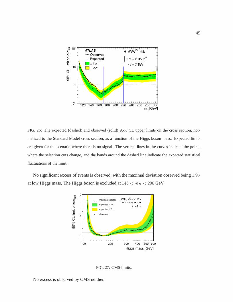
FIG. 26: The expected (dashed) and observed (solid) 95% CL upperlimits on the cross section, nor-
malized to the Standard Model cross section, as a function of the Higgs boson mass. Expected limits
are given for the scenario where there is no signal. The vertical lines in the curves indicate the points
where the selection cuts change, and the bands around the dashed line indicate the expected statistical
fluctuations of the limit.
No significant excess of events is observed, with the maximaldeviation observed being1.9σ
at low Higgs mass. The Higgs boson is excluded at145 < mH < 206 GeV.
FIG. 27: CMS limits.
No excess is observed by CMS neither.

46
B. H → ZZ∗ → 4ℓH → ZZ∗ → 4ℓH → ZZ∗ → 4ℓ channel.
A search for the SM Higgs boson has been done with the ATLAS detector in the channel
H → ZZ∗ → ℓ+ℓ−ℓ′+ℓ′− with ℓ, ℓ′ = e, µ. The analysis was performed with4.8 fb−1 of
luminosity inpp collisions at√
s = 7 TeV. The decay modeH → ZZ is the second dominant
for massesmH > 160 GeV, and with a BR larger than10−2 for mH > 120 GeV, as seen in
Fig. 4. In addition, in Fig 13 we see that the decay modeH → ZZ∗ → ℓ+ℓ−ℓ′+ℓ′− has aσBR
value between10−3 and10−2 pb in a very large range of Higgs masses, including the low mass
region. This makes the decay mode very important.
[GeV]4lm100 150 200 250
Eve
nts/
5 G
eV
0
2
4
6
8
10
-1Ldt = 4.8 fb∫ = 7 TeVs
4l→(*)ZZ→H
DATABackground
=125 GeV)H
Signal (m=150 GeV)
HSignal (m
=190 GeV)H
Signal (m
PreliminaryATLAS
[GeV]4lm200 400 600
Eve
nts/
10 G
eV
0
2
4
6
8
10
12
-1Ldt = 4.8 fb∫ = 7 TeVs
4l→(*)ZZ→H
DATABackground
=150 GeV)H
Signal (m=190 GeV)
HSignal (m
=360 GeV)H
Signal (m
PreliminaryATLAS
FIG. 28:m4l distribution of the selected candidates, compared to the background expectation. Error bars
represent 68.3% central confidence intervals. The signal expectation for severalmH hypotheses is also
shown.
Them4ℓ distribution for the total background and several signal hypotheses is compared to
the date in Fig. 28.

47
[GeV]Hm110 120 130 140 150 160 170 180
SM
σ/σ95
% C
L lim
it on
1
10
210
sObserved CL
sExpected CL
σ 1 ±σ 2 ±
PreliminaryATLAS 4l→(*)
ZZ→H-1Ldt = 4.8 fb∫
=7 TeVs
sObserved CL
sExpected CL
σ 1 ±σ 2 ±
[GeV]Hm200 250 300 350 400 450 500 550 600
SM
σ/σ95
% C
L lim
it on
1
10
210
sObserved CL
sExpected CL
σ 1 ±σ 2 ±
PreliminaryATLAS 4l→(*)
ZZ→H-1Ldt = 4.8 fb∫
=7 TeVs
sObserved CL
sExpected CL
σ 1 ±σ 2 ±
FIG. 29: The expected (dashed) and observed (full line)95% CL upper limits on the Higgs boson produc-
tion cross section as a function of the Higgs boson mass, divided by the expected SM Higgs boson cross
section. The green and yellow bands indicate the expected sensitivity with±1σ and±2σ fluctuations,
respectively.
Fig. 29 shows the expected and observed95% c.l. cross sections upper limits as a function
of mH . The SM Higgs boson is excluded at95% c.l. in the mass ranges135 < mH < 156 GeV,
181 < mH < 234 GeV, and255 < mH < 415 GeV.
The most significant deviations from the background-only hypothesis are observed formH =
125 GeV with2.1σ, mH = 244 GeV with2.3σ, andmH = 500 GeV with2.2σ.

48
FIG. 30: Event display of a4µ candidate event withm4l = 124.6 GeV. The masses of the lepton pairs
are 89.7 GeV and 24.6 GeV.
In Fig. 30 we show an ATLAS4µ event. The pair of muons coming from the on-shellZ has
an invariant mass of89.7 GeV, while the off-shellZ has an invariant mass of24.6 GeV. One of
the muons is detected by a Thin Gap Chamber.
49
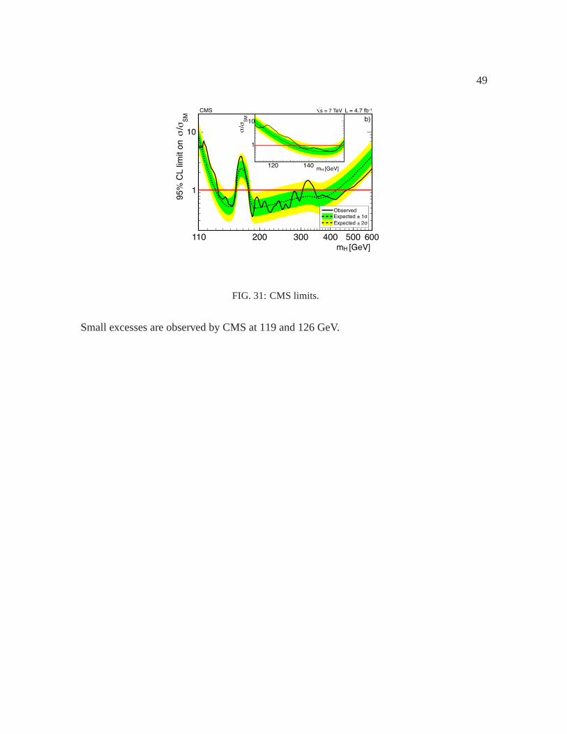
FIG. 31: CMS limits.
Small excesses are observed by CMS at 119 and 126 GeV.

50
C. H → γγH → γγH → γγ channel.
A search for the SM Higgs boson was done with the ATLAS Detector in the channelH →γγ, with 4.9 fb−1 of integrated luminosity withpp collisions at
√s = 7 TeV. In Fig. 4 we see
that the branching ratioB(H → γγ) is of the order10−3, with aσ × BR value between10−2
and10−1 pb, as seen in Fig 13. It is one of the most important decay modes in the low mass
region.
Events are required to contain a primary vertex with at leastthree tracks withpT > 0.4
GeV. TheET of the leading and sub-leading photon is required to be larger than 40 and 25
GeV respectively. The photon identification efficiency ranges typically from65% to 95% for
ET between 25 to 80 GeV.
[GeV]γγm
100 110 120 130 140 150 160
Dat
a -
Bkg
mod
el
-100-50
050
100100 110 120 130 140 150 160
Eve
nts
/ 1 G
eV
0
100
200
300
400
500
600
700
800
Data 2011Background model
= 120 GeV (MC)H
SM Higgs boson m
Inclusive diphoton sample
-1 Ldt = 4.9 fb∫ = 7 TeV, s
ATLAS Preliminary
FIG. 32: Invariant mass distribution for the inclusive data sample, overlaidwith the sum of the
background-only fit and the signal expectation for a mass hypothesis of120 GeV corresponding to the
SM cross section. The figure below displays the residual of the data with respect to the background-only
fit sum.
In Fig. 32 we plot the di-photon mass distributionmγγ for the about 22500 events passing

51
the selection in the range100 < mγγ < 160 GeV. The red solid line indicates the background
only scenario. Also shown is the signal expectation for a SM Higgs boson with mass 120 GeV.
Notice the excess of events near 125 GeV.
[GeV]Hm
110 115 120 125 130 135 140 145 150
S
Mσ/σ
95%
CL
limit
on
1
2
3
4
5
6
7
8 limitsObserved CL limit
sExpected CL
σ 1±σ 2±
ATLAS Preliminaryγγ →H
= 7 TeVsData 2011,
-1Ldt = 4.9 fb∫
FIG. 33: The observed and expected95% confidence level limits, normalised to the SM Higgs boson
cross sections, as a function of the hypothesized Higgs boson mass.
In Fig. 33 we see the95% c.l. limits on the ratio of the inclusive production cross section of
a SM-like Higgs boson relative to the SM model cross section.Very small Higgs mass regions
are ruled out:114 < mH < 115 GeV and135 < mH < 136 GeV. Over the di-photon mass
range110 < mγγ < 150 GeV the maximum deviation from the background-only expectation is
observed at 126 GeV, with a local significance of2.8 standard deviations.

52
FIG. 34: CMS limits.
CMS sees an excess at 124 GeV.

53
D. ATLAS and CMS: all channels combined
A preliminary combination of SM Higgs searches with the ATLAS Experiment has been
made, with a dataset corresponding to an integrated luminosity of up to4.9 fb−1 of pp collisions
collected at√
s = 7 TeV at the LHC.
[GeV]HM100 200 300 400 500 600
SM
σ/σ95
% C
L Li
mit
on
-110
1
10
ObservedExpected
σ1 ±σ2 ± = 7 TeVs
-1 Ldt = 1.0-4.9 fb∫ATLAS Preliminary 2011 Data
CLs Limits
[GeV]HM110 115 120 125 130 135 140 145 150
SM
σ/σ95
% C
L Li
mit
on
1
10ObservedExpected
σ1 ±σ2 ± = 7 TeVs
-1 Ldt = 1.0-4.9 fb∫ATLAS Preliminary 2011 Data
CLs Limits
FIG. 35: The combined upper limit on the Standard Model Higgs boson production cross section divided
by the Standard Model expectation as a function ofmH is indicated by the solid line. This is a95% CL
limit using the CLs method in the entire mass range. The dotted line shows the median expected limit in
the absence of a signal and the green and yellow bands reflect the corresponding68% and95% expected
regions.

54
The combination, in terms of the observed and expected upperlimits at the95% c.l. on the
Higgs boson production cross section, normalized to the SM value, of all channels is shown in
Fig. 35. The observed95% c.l. exclusion regions are112.7 < mH < 115.5 GeV,131 < mH <
237 GeV, and251 < mH < 468 GeV.
An excess of events is observed atmH = 126 GeV with a local significance of3.6σ, di-
minishing to2.2σ with the look elsewhere effect in the interval110 − 600 GeV. This excess is
observed by ATLAS in the three channels:H → γγ with 2.8σ, H → ZZ∗ → ℓ+ℓ−ℓ′+ℓ′− with
2.1σ, andH → WW ∗ → ℓ+νℓ′−ν with 1.4σ.
CMS Collaboration has also reported a smaller excess compatible with a SM Higgs boson
with mass in the vicinity of 124 GeV and below, with a local significance of3.1σ, diminishing
to 2.1σ if the mass interval is110 − 145 GeV, or to1.5σ for the full interval110 − 600 GeV.
FIG. 36: CMS limit.

55
XV. FINAL REMARKS
FIG. 37: ATLAS Collaboration.
• More data is needed to study this excess.
• 2012 is the year when the Higgs boson most likely will either be discovered or ruled out.
• If the excess at 125 GeV is confirmed as a new particle consistent with the Higgs boson,
we would have given the first step to understand the mechanismby which gauge bosons
and elementary fermions acquire mass.
Related Documents