Physics of Conductive Conjugated Polymers∗

GENERAL ARTICLE

Physics of Conductive Conjugated Polymers∗

A Primer

Hemanth K Bilihalli

Hemanth K Bilihalli obtained

his PhD in Chemical

Engineering from Indian

Institute of Technology

Madras in 2013. The PhD

work at IIT Madras exposed

the author to simple ab initio

‘jellium’ and

‘pseudopotential’ models of

metals. The present work was

completed during a tenure of

Assistant Professorship at

R.V College of Engineering,

Bengaluru.

In this expository article, the importance of electron-phonon

coupling to charge transport in conductive polymers—as a

result of a vanishing dynamic bandgap—is outlined. The au-

thor’s interpretation of physical models for this process: mod-

els are presented for predicting the conduction modes acti-

vated during charge transport.

1. Foreword

The well-known Huckel rule of physical chemistry states that or-

ganic rings with (4n + 2) electrons in Π-bonded orbitals exhibit

‘resonance’ or ‘delocalization’ of electrons. A similar condi-

tion holds in linear conjugated oligomers with half this number

of Π-bonded electrons, with facility for charge transport, in the

presence of ‘dopant’. Thus, it came as a surprise in 1977 that

long conjugated organic polymers were found to conduct elec-

tricity when polyacetylene was prepared by accidental addition

of ≈1000 times the required amount of the polymerization cat-

alyst (acting as a dopant). The practical applications of conduc-

tive polymers are—to quote the public announcement of the 2000

Chemistry Nobel Prize [1],

“...in low-cost manufacturing using solution-processing

of film-forming polymers. Light displays and inte-

grated circuits, for example, could theoretically be

manufactured using simple inkjet printer techniques.” Keywords

Phonon-electron interactions, lo-

calization effects, hopping trans-

port, Le polymers.Some examples of commercially employed conductive polymers

∗Vol.25, No.7, DOI: https://doi.org/10.1007/s12045-020-1011-1

RESONANCE | July 2020 947

GENERAL ARTICLE

are: polyaniline, poly(ethylenedioxythiophene), poly(phenylene

vinylidene), poly(dialkylfluorene), poly(thiophene), poly(pyrrole),

etc. These are primarily employed in anti-static coatings for elec-

tronic circuits, and sometimes in transistors and capacitors. More

recently, electroluminescent polymers have been discovered [poly(p-

phenylene vinylene) in 1990] that can form the active layers in

light emitting diodes (LEDs).

Apart from their technological impact, research on these materi-

als has proven to be fertile ground for testing novel theories on

conduction-insulation transition.

A cursory overview of conducting polymer structure via Raman

spectrum analysis reveals a small (but electrically significant) al-

ternation in bond length along the polymer chain (≈0.08Å in the

case of polyacetylene) [2], contrary to the “resonance school of

thought” about such conjugated systems.

One of the themes of this article, is the physics of coupling be-

tween the electron and the crystal lattice, in addition to the peda-

gogical aim of explaining charge conduction in terms of ‘a band-

gap eliminating midgap state’. This refers to an electronic state

forming in the middle of the forbidden region between the con-

duction and the valence bands of the semiconductor structure of

a polymer obtained by standard band structure calculation (see

Figure 8, also cf. Figure 3).

Although the theory of Su, Schrieffer, and Heeger [2] was worked

out soon (1980) after the discovery (1977) of these uncharacter-

istic materials, full justice with further treatment than provided

here demands a foray into the quantum mechanics of two-electron

interactions, suitably wrapped in the language of ‘second quanti-

zation’, for which advanced material, e.g. Altland and Simons’

book Condensed Matter Field Theory [3], must be consulted.

Instead, this article will verbalize the physical arguments that

signal the chemical changes occurring in conjugated polymers

and eventually facilitate the curious phenomenon of charge con-

duction. Section 2 is a first look at the electronic structure of

electron-rich periodic lattices, and the only mathematical proof

948 RESONANCE | July 2020

GENERAL ARTICLE

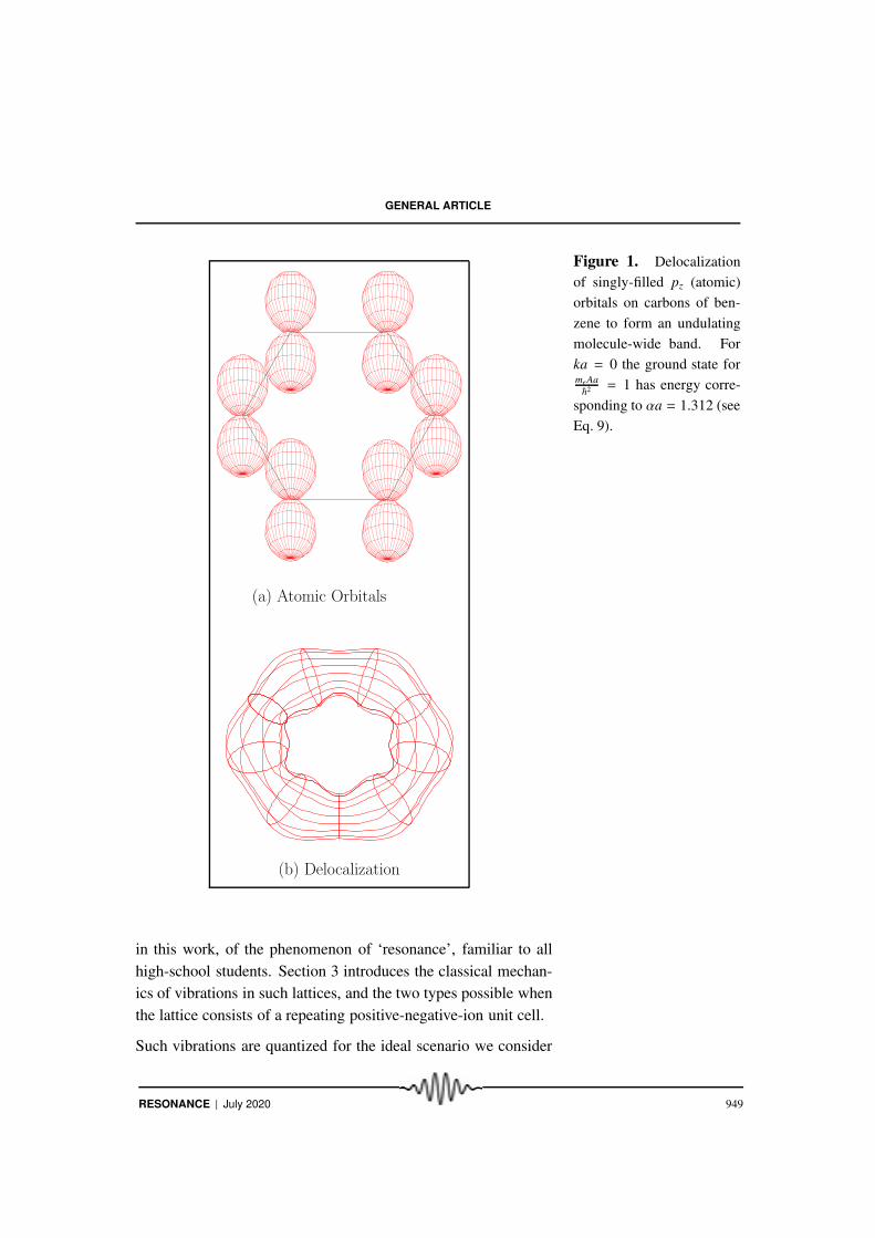
Figure 1. Delocalization

of singly-filled pz (atomic)

orbitals on carbons of ben-

zene to form an undulating

molecule-wide band. For

ka = 0 the ground state formeAa

~2 = 1 has energy corre-

sponding to αa = 1.312 (see

Eq. 9).

(a) Atomic Orbitals

(b) Delocalization

in this work, of the phenomenon of ‘resonance’, familiar to all

high-school students. Section 3 introduces the classical mechan-

ics of vibrations in such lattices, and the two types possible when

the lattice consists of a repeating positive-negative-ion unit cell.

Such vibrations are quantized for the ideal scenario we consider


GENERAL ARTICLE

Figure 2. trans-

polyacetylene in insulating

(top) and nearly-conducting

(bottom) forms. A neutral

‘soliton’ (‘kink’ in center,

S in Figure 8) forms in the

latter case, due to a ‘Peierls

instability’ [3].

a-d

d

here—even the smallest degree of vibration has a ‘zero-point en-

ergy’ [4]— and are then known by the quantum mechanical term

‘phonons’. Section 4 is a syncretism of Sections 2 and 3 and

specifies the‘rules’ that these quantized vibrations must follow,

including the ‘common-sensical rule’ of energy conservation. In

Section 5, we introduce the first signatures of a current-producing

non-equilibrium state: ‘localization’ and ‘soliton’. In analogy

with ‘semiclassical dynamical theories’ [5] of solid-state (e.g.

silicon-based) semiconductors, any realization of a finite current

generating non-equilibrium state is possible when quantum me-

chanical dynamics is also included in the governing model(s).

Such topics are deemed too advanced for our overview, so we

draw analogies for these concepts from classical counterparts. Fi-

nally, Section 6 hints at the soliton pair (‘polaron’) production

process induced by the addition of an external charge/application

of external potential. Here we sketch an argument due to Sethna

[6], supported by figures, for the charge transport mechanism of

pairwise electron hopping.

2. Periodicity, Tunneling/Resonance [7]

WeΠ-electrons in a

conjugated (i.e.

alternating double-single

bond) molecule such as

benzene undergoes

‘hybridization’ and

subsequently, resonance.

start with a familiar high school principle which teaches us

that theΠ-electrons in a conjugated (i.e. alternating double-single

bond) molecule such as benzene undergoes ‘hybridization’ and

subsequently, resonance. The pz orbital on each carbon atom

has a free electron which chooses to delocalize over the entire


GENERAL ARTICLE

Figure 3. Band structure

of a lattice ring of point (δ-

potential) ions.

0 5

10αa 0

5 10

15

meA/α-h2

0 0.5

1 1.5

2 2.5

3 3.5

ka

molecule and form, along with the other five pz electrons, a tubu-

lar orbital (‘energy band’), spread over the entire benzene ring.

The root cause of this is the quantum mechanical process of ‘tun-

neling’. In this section, we present an elementary discussion of

the process of energy band formation, starting from the Schrodinger

equation.

At a first level of approximation, the benzene molecule is a lattice

ring of point (δ potential) ions.

Being periodic, one may expand the wave function on this lattice

in a fourier series

ψk(x) =∑

K

uk(K)ei(k+K)x, (1)

where K is restricted to integer multiples of 2πa

, a being the ‘lattice

constant’ (or ion-ion separation).

The Schrodinger equation for the wave function of the electron

Hψk = Ekψk, (2)

thus reduces to

−~

2

2me

d2ψk

dx2+ V(x)ψk(x) = Ekψk (3)

⇒

[

~2(k + K)2

2me

− Ek

]

uk(K) +∑

K′

V(K − K′)uk(K′) = 0.


GENERAL ARTICLE

Substituting the fourier transform of V(x) = A∑∞

n=−∞ δ(x − na),

V(K) =1

a

∫ a/2

−a/2

dxV(x)e−iKx =A

a, (4)

into the above yields

[

~2(k + K)2

2me

− Ek

]

uk(K) +A

a

∑

K′

uk(K′) = 0. (5)

Solving for uk(K)

uk(K)∑

K′ uk(K′)=

2πA/(a~2)

2πmeEk/~2 − (k + K)2

, (6)

and summing over K yields an identity (LHS=1) and a relation

between Ek and k (‘band structure’). Defining α2 ≡ 2meEk/~2

and replacing the sum over K to one over index n, the above iden-

tity simplifies to

~2a

2meA=

∞∑

n=−∞

1

α2 −(

k + 2πna

)2

= −a

4α

∞∑

n=−∞

1

πn + ka2− αa

2

−1

πn + ka2+ αa

2

. (7)

Here we use a mathematical trick

cot x =

∞∑

n=−∞

1

nπ + x, (8)

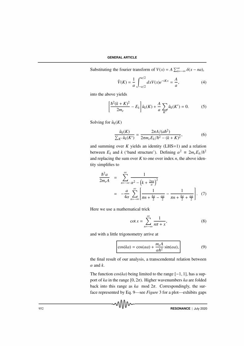
and with a little trigonometry arrive at

cos(ka) = cos(αa) +meA

α~2sin(αa), (9)

the final result of our analysis, a transcendental relation between

α and k.

The function cos(ka) being limited to the range [−1, 1], has a sup-

port of ka in the range [0, 2π). Higher wavenumbers ka are folded

back into this range as ka mod 2π. Correspondingly, the sur-

face represented by Eq. 9—see Figure 3 for a plot—exhibits gaps


GENERAL ARTICLE

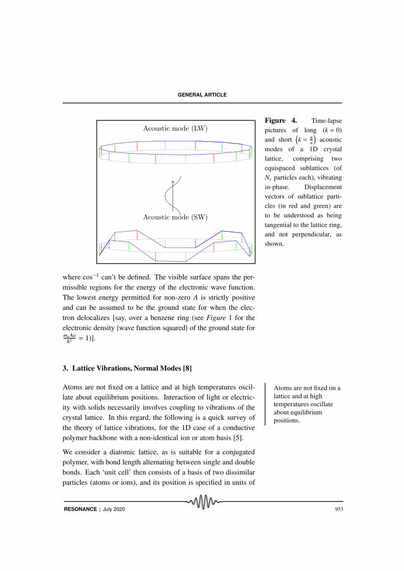
Figure 4. Time-lapse

pictures of long (k = 0)

and short(

k = π

a

)

acoustic

modes of a 1D crystal

lattice, comprising two

equispaced sublattices (of

Nc particles each), vibrating

in-phase. Displacement

vectors of sublattice parti-

cles (in red and green) are

to be understood as being

tangential to the lattice ring,

and not perpendicular, as

shown.

Acoustic mode (LW)

Acoustic mode (SW)

where cos−1 can’t be defined. The visible surface spans the per-

missible regions for the energy of the electronic wave function.

The lowest energy permitted for non-zero A is strictly positive

and can be assumed to be the ground state for when the elec-

tron delocalizes [say, over a benzene ring (see Figure 1 for the

electronic density {wave function squared} of the ground state formeAa

~2 = 1)].

3. Lattice Vibrations, Normal Modes [8]

Atoms Atoms are not fixed on a

lattice and at high

temperatures oscillate

about equilibrium

positions.

are not fixed on a lattice and at high temperatures oscil-

late about equilibrium positions. Interaction of light or electric-

ity with solids necessarily involves coupling to vibrations of the

crystal lattice. In this regard, the following is a quick survey of

the theory of lattice vibrations, for the 1D case of a conductive

polymer backbone with a non-identical ion or atom basis [5].

We consider a diatomic lattice, as is suitable for a conjugated

polymer, with bond length alternating between single and double

bonds. Each ‘unit cell’ then consists of a basis of two dissimilar

particles (atoms or ions), and its position is specified in units of


GENERAL ARTICLE

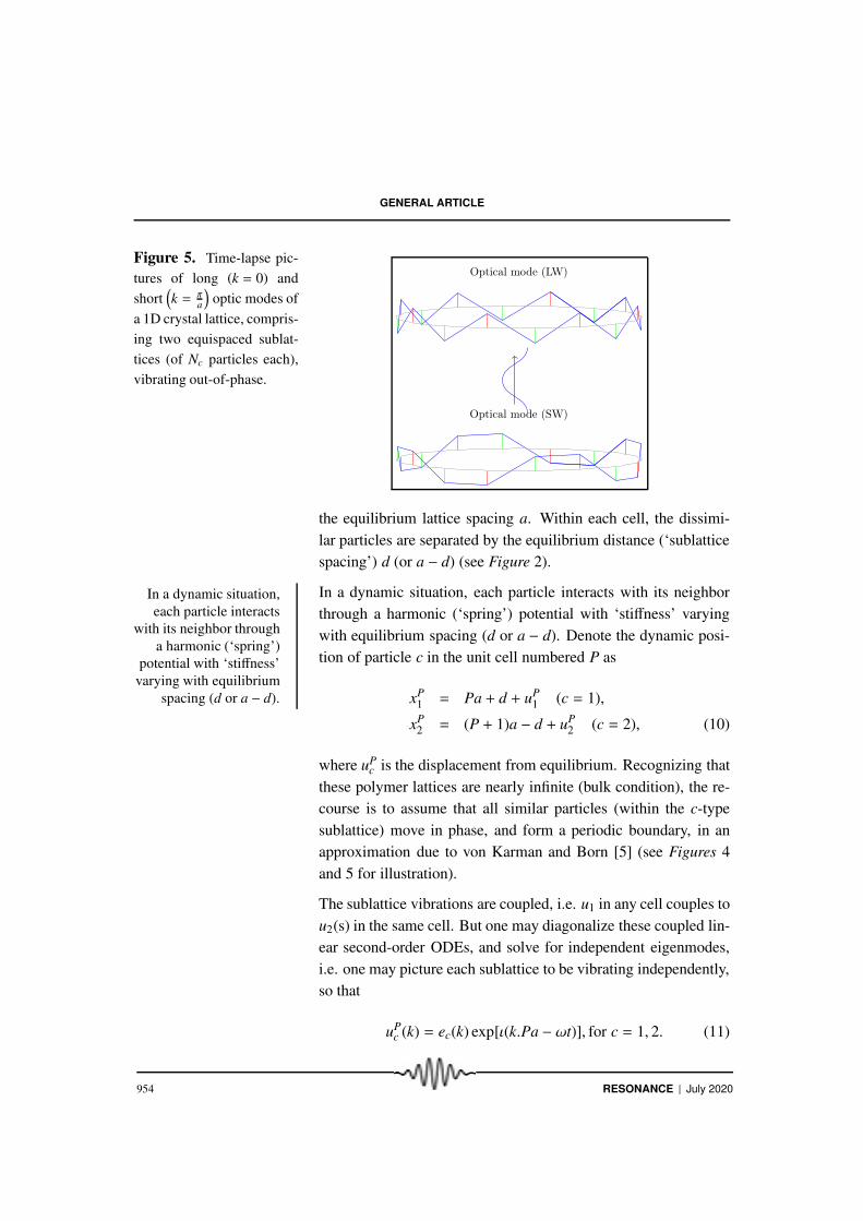
Figure 5. Time-lapse pic-

tures of long (k = 0) and

short(

k = π

a

)

optic modes of

a 1D crystal lattice, compris-

ing two equispaced sublat-

tices (of Nc particles each),

vibrating out-of-phase.

Optical mode (LW)

Optical mode (SW)

the equilibrium lattice spacing a. Within each cell, the dissimi-

lar particles are separated by the equilibrium distance (‘sublattice

spacing’) d (or a − d) (see Figure 2).

InIn a dynamic situation,

each particle interacts

with its neighbor through

a harmonic (‘spring’)

potential with ‘stiffness’

varying with equilibrium

spacing (d or a − d).

a dynamic situation, each particle interacts with its neighbor

through a harmonic (‘spring’) potential with ‘stiffness’ varying

with equilibrium spacing (d or a − d). Denote the dynamic posi-

tion of particle c in the unit cell numbered P as

xP1 = Pa + d + uP

1 (c = 1),

xP2 = (P + 1)a − d + uP

2 (c = 2), (10)

where uPc is the displacement from equilibrium. Recognizing that

these polymer lattices are nearly infinite (bulk condition), the re-

course is to assume that all similar particles (within the c-type

sublattice) move in phase, and form a periodic boundary, in an

approximation due to von Karman and Born [5] (see Figures 4

and 5 for illustration).

The sublattice vibrations are coupled, i.e. u1 in any cell couples to

u2(s) in the same cell. But one may diagonalize these coupled lin-

ear second-order ODEs, and solve for independent eigenmodes,

i.e. one may picture each sublattice to be vibrating independently,

so that

uPc (k) = ec(k) exp[ι(k.Pa − ωt)], for c = 1, 2. (11)


GENERAL ARTICLE

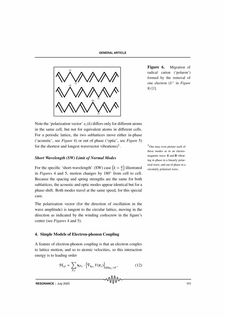
Figure 6. Migration of

radical cation (‘polaron’)

formed by the removal of

one electron (S + in Figure

8) [1].

+

◦+

◦+

◦

Note the ‘polarization vector’ ec(k) differs only for different atoms

in the same cell, but not for equivalent atoms in different cells.

For a periodic lattice, the two sublattices move either in-phase

(‘acoustic’, see Figure 4) or out of phase (‘optic’, see Figure 5)

for the shortest and longest wavevector vibrations)1 1One may even picture each of

these modes as in an electro-

magnetic wave: E and B vibrat-

ing in phase in a linearly polar-

ized wave, and out of phase in a

circularly polarized wave.

.

Short Wavelength (SW) Limit of Normal Modes

For the specific ‘short-wavelength’ (SW) case(

k = πa

)

illustrated

in Figures 4 and 5, motion changes by 180◦ from cell to cell.

Because the spacing and spring strengths are the same for both

sublattices, the acoustic and optic modes appear identical but for a

phase-shift. Both modes travel at the same speed, for this special

case.

The polarization vector (for the direction of oscillation in the

wave amplitude) is tangent to the circular lattice, moving in the

direction as indicated by the winding corkscrew in the figure’s

center (see Figures 4 and 5).

4. Simple Models of Electron-phonon Coupling

A feature of electron-phonon coupling is that an electron couples

to lattice motion, and so to atomic velocities, so this interaction

energy is to leading order

Hep =∑

P,c

xP,c ·[

∇xP,cV(re)

]

allxP,c=0, (12)


GENERAL ARTICLE

where re are electronic coordinates, V(re) is the electron-ion in-

teraction referred to in Section 2. Now, as the lattice is peri-

odic, and only nearest neighbor atoms/ions interact, an electron

of wavevector k is transformed into wavevector k′ subject to con-

servation of wavevector addition or subtraction to a wavevector b

in the ‘reciprocal lattice’,

k′ − k − q = b. (13)

With the additional assumption that the electrons respond instan-

taneously to ionic movement, one may also derive the condition

that optic phonons do not affect electrons while acoustic phonons

do (see Appendix N of [5] or [9] for proof). Patterson and Bailey

[9] offer the qualitative explanation:

“...in optic modes the adjacent atoms tend to vibrate

in opposite directions, and so the net effect of the

vibrations tends to be very small due to cancellation

[cf. with Figure 5]”.

Finally, in all cases, the energy conservation rule

Ek′ = Ek + ~ω(q) (14)

must be satisfied [9].

5. Non-equilibrium States and Solitons

In the non-equilibrium state, the picture of particle dynamics pre-

sented in Figures 4 and 5 deviates from the actual dynamics pre-

sented in Figure 6 primarily due to quantum mechanical reasons

of ‘localization’ [10]. This means that the soliton shape of parti-

cle motion is an attenuated beat pattern—quite like the emblem

of Resonance!—best characterized as classical shuttling of a par-

ticle between two wells separated by a metastable barrier. The

classical ‘sine-Gordon soliton’ is the continuum representation

of coupled pendula (refer to Figure 7) in a vertical gravitational

field with (cone-shaped) neighboring bobs strung together with


GENERAL ARTICLE

Figure 7. A topological

soliton in classical mechan-

ics. The conical pendulum

bobs are in dynamic equilib-

rium as the locus of inexten-

sible cords stringing them

together winds over the sus-

pension rod and swings be-

tween positions of lowest

overall energy in a gravita-

tional field.

Top view

Front view

Isometric view

Side view

inextensible cords. However, sine-Gordon dynamics fluctuate

between angular positions (180◦ apart) of energy minima in the

gravitational field, whereas a soliton fluctuates between minima

of the classical ‘action’—the equivalent of the energy to be mini-

mized in (position, momentum)—space.

This does not mean that Figure 4 is completely irrelevant. Soli-

tons of somewhat smaller sizes [L ≈ 6 bond lengths for poly-

acetylene [2] ψ ∼ sech(

xL

)

cos(

πxa

)

] form the backbone of elec-

tronic structure studies of conductive polymers [11]. These are

modulated at the band edges k = πa

to preserve the periodic sym-

metry of the excitation. Furthermore these may be of the ‘topo-

logical type’, exhibiting a ‘winding around’—just like the cou-

pled pendula in Figure 7—in state space, of an ‘action angle’

parametrizing the tunneling process.

6. Charge Transport

We stop at the penultimate topic in the process of formulation of

the successful model of Su–Schrieffer–Heeger and reiterate that

this is outside our purview. Instead, a layman’s description of the


GENERAL ARTICLE

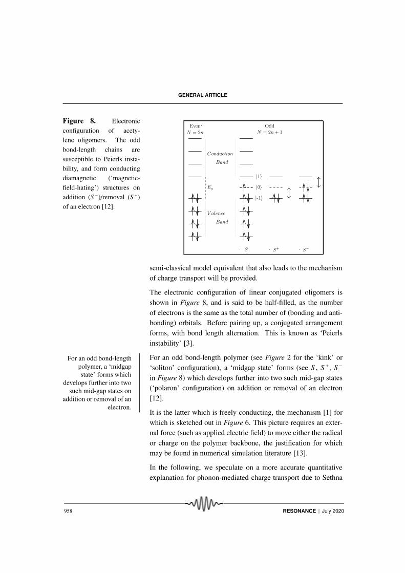
Figure 8. Electronic

configuration of acety-

lene oligomers. The odd

bond-length chains are

susceptible to Peierls insta-

bility, and form conducting

diamagnetic (‘magnetic-

field-hating’) structures on

addition (S −)/removal (S +)

of an electron [12].

Even

N = 2n

Eg

Conduction

Band

V alence

Band

S

|-1〉

|0〉

|1〉

Odd

N = 2n + 1

S+ S−

semi-classical model equivalent that also leads to the mechanism

of charge transport will be provided.

The electronic configuration of linear conjugated oligomers is

shown in Figure 8, and is said to be half-filled, as the number

of electrons is the same as the total number of (bonding and anti-

bonding) orbitals. Before pairing up, a conjugated arrangement

forms, with bond length alternation. This is known as ‘Peierls

instability’ [3].

ForFor an odd bond-length

polymer, a ‘midgap

state’ forms which

develops further into two

such mid-gap states on

addition or removal of an

electron.

an odd bond-length polymer (see Figure 2 for the ‘kink’ or

‘soliton’ configuration), a ‘midgap state’ forms (see S , S +, S −

in Figure 8) which develops further into two such mid-gap states

(‘polaron’ configuration) on addition or removal of an electron

[12].

It is the latter which is freely conducting, the mechanism [1] for

which is sketched out in Figure 6. This picture requires an exter-

nal force (such as applied electric field) to move either the radical

or charge on the polymer backbone, the justification for which

may be found in numerical simulation literature [13].

In the following, we speculate on a more accurate quantitative

explanation for phonon-mediated charge transport due to Sethna


GENERAL ARTICLE

Figure 9. Polymer lattice

relaxation as habiting elec-

tron pair transitions between

neighboring potential wells.

t = −∞

t = 0

t = ∞

[6]. Without delving into the physics of this model, we present

the reader with a (lay) description and a picture (Figure 9). The

actual mode of charge transport is considerably complex as re-

cently worked out computationally by Lin et al. [11].

Electrons Electrons under the

influence of the

phonon-coupling tend to

‘pair up’ and move

together in concert.

under the influence of the phonon-coupling tend to ‘pair

up’ and move together in concert. Sethna offers a vivid ‘rubber-

sheet analogy’ for the description of ‘self-trapping’ [6]:

“...the second electron see[s] the potential hole sunk

by the first, and together [makes] an even deeper hole.”

Further, as the electron pair attempts to ‘hop’ from one (nearly

quadratic) potential well to another, the polymer lattice adapts

to yield a joint (nearly quartic) potential with a broader well at

the middle of the transport process, so that the phonon relaxation

facilitates initially but traps finally (Figure 9). The reader may

wonder why the two electrons do not repel in their pair-like con-

figuration; one possible solution to this riddle is:

“The paired states are energetically favored, and elec-

trons go in and out of those states preferentially.”

quoting the Wikipedia entry [14] on similarly-paired electrons in

superconductivity.


GENERAL ARTICLE

7. Afterword

This article does not address the necessity of doping to induce

charge transport through soliton propagation. Nor does it explain

how midgap states induce the spontaneous formation of electron-

hole pairs (excitons) that can tunnel through for current transport.

As long as the conducting localized units (solitons or polarons

or bipolaron pairs) remain small compared to the polymer chain

length, the physics doesn’t change much, and models may be re-

tained by adjusting parameters [15] to fit experimental data and/or

simulation results.

The interested reader thrown off by jargon used here is encour-

aged to follow, with a little effort in matrix algebra and calculus,

the online exposition of Zhu [16], complete with illuminating fig-

ures, for details on second quantization, Peierls instability, and

topological solitons.

Acknowledgements

This study/review was completed under the COE Macroelectron-

ics initiative of a TEQIP-1.2 grant award for R.V College of En-

gineering, Bangalore. The author acknowledges encouragement

over the duration of the project from Sri. K.N. Raja Rao, TEQIP

coordinator, and Dr M. Uttara Kumari, Head, COE Macroelec-

tronics. The author also thanks Dr T. Gupta from the Department

of Physics for valuable comments on this work. Much rewriting

to mould this work to the pedagogical spirit of the journal was

initiated by the comments of the two reviewers, for which the au-

thor is grateful. Finally the author unflinchingly admits this work

would not have seen the light of day if not for the personal de-

liberations with Dr M.S. Ananth of IIT Madras on the process of

science communication.

Suggested Reading

[1] B Norden and E Krutmeijer, The Nobel Prize in Chemistry, 2000: Conductive

Polymers, www.nobelprize.org


www.nobelprize.org

GENERAL ARTICLE

[2] W P Su, J R Schrieffer, and A J Heeger. Soliton excitations in polyacetylene,

Phys. Rev. B, Vol.22, p.2099, 1980.

[3] A Altland and B Simons, Condensed Matter Field Theory, Cambridge, 2010.

[4] Wikipedia contributors, Zero-point energy, Wikipedia: The Free Encyclopedia,

https://en.wikipedia.org/wiki/Zero-point_energy

[5] N W Ashcroft and N D Mermin, Solid State Physics, Brooks-Cole, 1976.

[6] J P Sethna, Phonon coupling in tunneling systems at zero temperature: An

instanton approach, Phys. Rev. B, Vol.24, p.698, 1981.

[7] Wikipedia contributors,

Particle in a one-dimensional lattice—Wikipedia, The Free Encyclopedia,

http://en.wikipedia.org/wiki/Particle_in_a_one-dimensional_lattice

[8] L D Landau and E M Lifshitz, Statistical Physics Part 1, Volume 5: Course of

Theoretical Physics, Elsevier, 1980.

[9] J D Patterson and B C Bailey, Solid-State Physics: Introduction to the Theory,

Springer, 2010.

[10] P W Anderson. The size of localized states near the mobility edge, Proc. Natl.

Acad. Sci. USA, Vol.69, p.1097, 1972.

[11] X Lin, J Li, C J Forst and S Yip, Multiple self-localized electronic states in

trans-polyacetylene, Proc. Natl. Acad. Sci. USA, Vol.103, p.8943, 2006.

[12] Z Soos and L R Ducasse, Electronic correlations and midgap absorption in

polyacetylene, J. Phys. (Paris), Vol.44, C3-467, 1983.

Address for Correspondence

Hemanth K Bilihalli

56, 8th Cross

R.K. Layout, 1st Stage

Padmanabhanagar

Bengaluru 560 070

Email:

[email protected]

[13] C Kuhn, Solitons, polarons, and excitons in polyacetylene: Step-potential

model for electron-phonon coupling in pi-electron systems, Phys. Rev. B, Vol.40,

p.7776, 1989.

[14] Wikipedia contributors, Cooper pair, Wikipedia: The Free Encyclopedia,

https://en.wikipedia.org/wiki/Cooper_pair

[15] P W Anderson, Model for the electronic structure of amorphous semiconduc-

tors, Phys. Rev. Lett., Vol.34, p.953, 1975.

[16] B C Zhu, Lecture 1: 1-d SSH model— Physics 0.1 Documentation,

phyx.readthedocs.io/en/latest/TI/Lecture%20notes/1.html 2014.


https://en.wikipedia.org/wiki/Zero-point_energy

http://en.wikipedia.org/wiki/Particle_in_a_one-dimensional_lattice

https://en.wikipedia.org/wiki/Cooper_pair

phyx.readthedocs.io/en/latest/TI/Lecture%20notes/1.html

Physics of Conductive Conjugated Polymers∗

Documents