Physics of Classical Electromagnetism · The Maxwell theory of electromagnetism was well established in the latter nine-teenth century, when H. R. Hertz demonstrated the electromagnetic

Physics of Classical Electromagnetism

Minoru Fujimoto

Physics of ClassicalElectromagnetism

Minoru FujimotoDepartment of PhysicsUniversity of GuelphGuelph, OntarioCanada, N1G 2W1

Library of Congress Control Number: 2007921094

ISBN: 978-0-387-68015-6 e-ISBN: 978-0-387-68018-7

Printed on acid-free paper.

C© 2007 Springer Science+Business Media, LLCAll rights reserved. This work may not be translated or copied in whole or in part without the writtenpermission of the publisher (Springer Science+Business Media, LLC, 233 Spring Street, New York,NY 10013, USA), except for brief excerpts in connection with reviews or scholarly analysis. Usein connection with any form of information storage and retrieval, electronic adaptation, computersoftware, or by similar or dissimilar methodology now known or hereafter developed is forbidden.The use in this publication of trade names, trademarks, service marks, and similar terms, even if theyare not identified as such, is not to be taken as an expression of opinion as to whether or not they aresubject to proprietary rights.

9 8 7 6 5 4 3 2 1

springer.com

Contents

Preface.................................................................................... xi

1. Steady Electric Currents ......................................................... 11.1. Introduction .................................................................. 11.2. Standards for Electric Voltages and Current ........................... 21.3. Ohm Law’s and Heat Energy ............................................. 41.4. The Kirchhoff Theorem.................................................... 8

PART 1. ELECTROSTATICS 13

2. Electrostatic Fields................................................................ 152.1. Static Charges and Their Interactions ................................... 152.2. A Transient Current and Static Charges ................................ 162.3. Uniform Electric Field in a Parallel-Plate Condenser ................ 19

2.3.1. The Electric Field Vector ......................................... 192.3.2. The Flux Density Vector .......................................... 21

2.4. Parallel and Series Connections of Capacitors ........................ 252.5. Insulating Materials ........................................................ 26

3. The Gauss Theorem .............................................................. 303.1. A Spherical Capacitor...................................................... 303.2. A Cylindrical Capacitor ................................................... 333.3. The Gauss Theorem ........................................................ 343.4. Boundary Conditions....................................................... 39

3.4.1. A Conducting Boundary .......................................... 393.4.2. A Dielectric Boundary ............................................ 40

4. The Laplace–Poisson Equations................................................ 434.1. The Electrostatic Potential ................................................ 434.2. The Gauss Theorem in Differential Form .............................. 444.3. Curvilinear Coordinates (1) ............................................... 46

v

vi Contents

4.4. The Laplace–Poisson Equations ......................................... 494.4.1. Boundary Conditions .............................................. 494.4.2. Uniqueness Theorem .............................................. 504.4.3. Green’s Function Method......................................... 51

4.5. Simple Examples............................................................ 534.6. The Coulomb Potential .................................................... 554.7. Point Charges and the Superposition Principle........................ 58

4.7.1. An Electric Image .................................................. 584.7.2. Electric Dipole Moment........................................... 604.7.3. The Dipole-Dipole Interaction................................... 63

5. The Legendre Expansion of Potentials ........................................ 645.1. The Laplace Equation in Spherical Coordinates ...................... 645.2. Series Expansion of the Coulomb Potential............................ 665.3. Legendre’s Polynomials ................................................... 685.4. A Conducting Sphere in a Uniform Field .............................. 695.5. A Dielectric Sphere in a Uniform Field................................. 715.6. A Point Charge Near a Grounded Conducting Sphere ............... 725.7. A Simple Quadrupole ...................................................... 755.8. Associated Legendre Polynomials ....................................... 765.9. Multipole Potentials ........................................................ 79

PART 2. ELECTROMAGNETISM 83

6. The Ampere Law.................................................................. 856.1. Introduction .................................................................. 856.2. The Ampere Law............................................................ 866.3. A Long Solenoid ............................................................ 896.4. Stokes’ Theorem ............................................................ 916.5. Curvilinear Coordinates (2) ............................................... 946.6. The Ampere Law in Differential Form.................................. 966.7. The Rowland Experiment ................................................. 98

7. Magnetic Induction ............................................................... 1017.1. Laws of Magnetic Induction .............................................. 101

7.1.1. The Faraday Law................................................... 1017.1.2. The Lenz Law....................................................... 1037.1.3. Magnetic Field Vectors............................................ 103

7.2. Differential Law of Induction and the Dynamic Electric Field..... 1047.3. Magnetic Moments ......................................................... 108

8. Scalar and Vector Potentials..................................................... 1128.1. Magnets....................................................................... 1128.2. Pohl’s Magnetic Potentiometer........................................... 114

Contents vii

8.3. Scalar Potentials of Magnets ............................................ 1168.3.1. A Laboratory Magnet........................................... 1168.3.2. A Uniformly Magnetized Sphere............................. 118

8.4. Vector Potentials........................................................... 1198.5. Examples of Steady Magnetic Fields .................................. 1218.6. Vector and Scalar Potentials of a Magnetic Moment ............... 1268.7. Magnetism of a Bohr’s Atom ........................................... 128

9. Inductances and Magnetic Energies ........................................... 1329.1. Inductances ................................................................. 1329.2. Self- and Mutual Inductances ........................................... 1359.3. Mutual Interaction Force Between Currents.......................... 1389.4. Examples of Mutual Induction.......................................... 139

9.4.1. Parallel Currents................................................. 1399.4.2. Two Ring Currents .............................................. 140

10. Time-Dependent Currents ...................................................... 14210.1. Continuity of Charge and Current...................................... 14210.2. Alternating Currents ...................................................... 14310.3. Impedances ................................................................. 14510.4. Complex Vector Diagrams............................................... 14710.5. Resonances ................................................................. 149

10.5.1. A Free LC Oscillation .......................................... 14910.5.2. Series Resonance ............................................... 15010.5.3. Parallel Resonance .............................................. 151

10.6. Four-Terminal Networks ................................................. 15210.6.1. RC Network ...................................................... 15310.6.2. Loaded Transformer ............................................ 15510.6.3. An Input-Output Relation in a Series RCL Circuit........ 15610.6.4. Free Oscillation in an RCL Circuit .......................... 157

PART 3. ELECTROMAGNETIC WAVES 159

11. Transmission Lines ............................................................... 16111.1. Self-Sustained Oscillators ............................................... 16111.2. Transmission Lines........................................................ 16311.3. Fourier Transforms........................................................ 16511.4. Reflection and Standing Waves ......................................... 16711.5. The Smith Chart ........................................................... 170

12. The Maxwell Equations ......................................................... 17212.1. The Maxwell Equations .................................................. 17212.2. Electromagnetic Energy and the Poynting Theorem................ 17512.3. Vector and Scalar Potentials............................................. 176

viii Contents

12.4. Retarded Potentials........................................................ 17712.5. Multipole Expansion...................................................... 180

13. Electromagnetic Radiation ...................................................... 18413.1. Dipole Antenna ............................................................ 18413.2. Electric Dipole Radiation ................................................ 18413.3. The Hertz Vector .......................................................... 18813.4. A Half-Wave Antenna .................................................... 19213.5. A Loop Antenna ........................................................... 19313.6. Plane Waves in Free Space .............................................. 195

14. The Special Theory of Relativity............................................... 19914.1. Newton’s Laws of Mechanics........................................... 19914.2. The Michelson–Morley Experiment ................................... 20014.3. The Lorentz Transformation ............................................ 20214.4. Velocity and Acceleration in Four-Dimensional Space ............ 20414.5. Relativistic Equation of Motion ........................................ 20614.6. The Electromagnetic Field in Four-Dimensional Space............ 208

15. Waves and Boundary Problems................................................. 21415.1. Skin Depths................................................................. 21415.2. Plane Electromagnetic Waves in a Conducting Medium........... 21615.3. Boundary Conditions for Propagating Waves........................ 21815.4. Reflection from a Conducting Boundary.............................. 21915.5. Dielectric Boundaries..................................................... 22115.6. The Fresnel Formula...................................................... 223

16. Guided Waves...................................................................... 22616.1. Propagation Between Parallel Conducting Plates ................... 22616.2. Uniform Waveguides ..................................................... 229

16.2.1. Transversal Modes of Propagation(TE and TM Modes)............................................ 229

16.2.2. Transversal Electric-Magnetic Modes (TEM) ............. 23216.3. Examples of Waveguides ................................................ 233

PART 4. COHERENT WAVES AND RADIATION QUANTA 241

17. Waveguide Transmission ........................................................ 24317.1. Orthogonality Relations of Waveguide Modes....................... 24317.2. Impedances ................................................................. 24517.3. Power Transmission Through a Waveguide .......................... 24917.4. Multiple Reflections in a Waveguide .................................. 250

18. Resonant Cavities ................................................................. 25318.1. Slater’s Theory of Normal Modes...................................... 25318.2. The Maxwell Equations in a Cavity.................................... 256

Contents ix

18.3. Free and Damped Oscillations .......................................... 25818.4. Input Impedance of a Cavity ............................................ 26018.5. Example of a Resonant Cavity.......................................... 26318.6. Measurements of a Cavity Resonance................................. 265

19. Electronic Excitation of Cavity Oscillations ................................. 26819.1. Electronic Admittance.................................................... 26819.2. A Klystron Cavity ......................................................... 27019.3. Velocity Modulation ...................................................... 27419.4. A Reflex Oscillator........................................................ 276

20. Dielectric and Magnetic Responses in Resonant Electromagnetic Fields 28020.1. Introduction................................................................. 28020.2. The Kramers–Kronig Formula.......................................... 28120.3. Dielectric Relaxation ..................................................... 28320.4. Magnetic Resonance ..................................................... 28820.5. The Bloch Theory ......................................................... 29020.6. Magnetic Susceptibility Measured by Resonance Experiments .. 292

21. Laser Oscillations, Phase Coherence, and Photons ......................... 29421.1. Optical Resonators ........................................................ 29421.2. Quantum Transitions...................................................... 29621.3. Inverted Population and the Negative Temperature ................. 29921.4. Ammonium Maser ........................................................ 30021.5. Coherent Light Emission from a Gas Laser .......................... 30121.6. Phase Coherence and Radiation Quanta .............................. 302

APPENDIX 305

Mathematical Notes .................................................................... 307A.1. Orthogonal Vector Space....................................................... 307A.2. Orthogonality of Legendre’s Polynomials .................................. 308A.3. Associated Legendre Polynomials............................................ 310A.4. Fourier Expansion and Wave Equations..................................... 312A.5. Bessel’s Functions ............................................................... 314

REFERENCES 317

Index ...................................................................................... 319

Preface

The Maxwell theory of electromagnetism was well established in the latter nine-teenth century, when H. R. Hertz demonstrated the electromagnetic wave. Thetheory laid the foundation for physical optics, from which the quantum conceptemerged for microscopic physics. Einstein realized that the speed of electromag-netic propagation is a universal constant, and thereby recognized the Maxwellequations to compose a fundamental law in all inertial systems of reference. Onthe other hand, the pressing demand for efficient radar systems during WWIIaccelerated studies on guided waves, resulting in today’s advanced telecommuni-cation technology, in addition to a new radio- and microwave spectroscopy. Thestudies were further extended to optical frequencies, and laser electronics and so-phisticated semi-conducting devices are now familiar in daily life. Owing to theseadvances, our knowledge of electromagnetic radiation has been significantly up-graded beyond plane waves in free space. Nevertheless, in the learning processthe basic theory remains founded upon early empirical rules, and the traditionalteaching should therefore be modernized according to priorities in the modern era.

In spite of the fact that there are many books available on this well-establishedtheme, I was motivated to write this book, reviewing the laws in terms of contem-porary knowledge in order to deal with modern applications. Here I followed twobasic guidelines. First, I considered electronic charge and spin as empirical in thedescription of electromagnetism. This is unlike the view of early physicists, whoconsidered these ideas hypothetical. Today we know they are factual, althoughstill unexplained from first principle. Second, the concept of “fields” should be inthe forefront of discussion, as introduced by Faraday. In these regards I benefitedfrom Professor Pohl’s textbook, Elektrizitatslehre, where I found a very stimu-lating approach. Owing a great deal to him, I was able to write my introductorychapters in a rather untraditional way, an approach I have found very useful inmy classes. In addition, in this book I discussed microwave and laser electronicsin some depth, areas where coherent radiation plays a significant role for moderntelecommunication.

I wrote this book primarily for students at upper undergraduate levels, hopingit would serve as a useful reference as well. I emphasized the physics of elec-tromagnetism, leaving mathematical details to writers of books on “mathematical

xi

xii Preface

physics.” Thus, I did not include sections for “mathematical exercise,” but I hopethat readers will go through the mathematical details in the text to enhance theirunderstanding of the physical content.

In Chapter 21 quantum transitions are discussed to an extent that aims to makeit understandable intuitively, although here I deviated from classical theories.Although this topic is necessary for a reader to deal with optical transitions, myintent was to discuss the limits of Maxwell’s classical theory that arise from phasecoherency in electromagnetic radiation.

It is a great pleasure to thank my students and colleagues, who assisted me bytaking part in numerous discussions and criticisms. I have benefited especially bycomments from S. Jerzak of York University, who took time to read the first draft.I am also grateful to J. Nauheimer who helped me find literature in the Germanlanguage. My appreciation goes also to Springer-Verlag for permission to use somefigures from R. W. Pohl’s book Elektrizitatslehre.

Finally, I thank my wife Haruko for her encouragement during my writing,without which this book could not have been completed.

M. FujimotoSeptember 2006

1Steady Electric Currents

1.1. Introduction

The macroscopic electric charge on a body is determined from the quantity ofelectricity carried by particles constituting the material. Although some electricphenomena were familiar before discoveries of these particles, such an origin ofelectricity came to our knowledge after numerous investigations of the structureof matter. Unlike the mass that represents mechanical properties, two kinds ofelectric charges different in sign were discovered in nature, signified by attractiveand repulsive interactions between charged bodies. While electric charges can becombined as in algebraic addition, carrier particles tend to form neutral species inequilibrium states of matter, corresponding to zero of the charge in macroscopicscale.

Frictional electricity, for example, represents properties of rubbed bodies arisingfrom a structural change on the surfaces, which is unrelated to their masses. Also,after Oersted’s discovery it was known that the magnetic field is related to movingcharges. It is well established that electricity and magnetism are not independentphenomena, although they were believed to be so in early physics. Today, suchparticles as electrons and atomic nuclei are known as basic elements composedof masses and charges of materials, as substantiated in modern chemistry. Theelectromagnetic nature of matter can therefore be attributed to these particleswithin accuracies of modern measurements. In this context we can express the lawof electromagnetism more appropriately than following in the footsteps in earlyphysics.

Today, we are familiar with various sources of electricity besides by friction.Batteries, for example, a modern version of Volta’s pile1, are widely used in dailylife as sources of steady electric currents. Also familiar is alternating current (AC)that can be produced when a mechanical work is converted to an induction currentin a magnetic field. Supported by contemporary chemistry, in all processes where

1 Volta’s pile was constructed in multi-layers of Zn and Cu plates sandwiched alternatelywith wet rags. Using such a battery, he was able to produce a relatively high emf for a weakcurrent by today’s standard.

1

2 1. Steady Electric Currents

electricity is generated, we note that positive and negative charges are separatedfrom neutral matter at the expense of internal and external energies. Positive andnegative charges ±Q are thus produced simultaneously in equal quantities, wherethe rate dQ/dt , called the electric current, is a significant quantity for electricalenergies to be used for external work. Traditionally, the current source is charac-terized by an electromotive force, or “emf,” to signify the driving force, which isnow expressed by the potential energy of the source.

Historically, Volta’s invention of an electric pile (ca. 1799) played an importantrole in producing steady currents, which led Oersted and Ampere to discoveries ofthe fundamental relation between current and magnetic fields (1820). In such earlyexperiments with primitive batteries, these pioneers found the law of the magneticfield by using small compass needles placed near the current. Today, the magneticfield can be measured with an “ammeter” that indicates an induced current. Inaddition to the electron spin discovered much later, it is now well established thatcharges in motion are responsible for magnetic fields, and all electrical quantitiescan be expressed in practical units of emf and current. As they are derived fromprecision measurements, these units are most suitable for formulating the laws ofelectromagnetism.

On the other hand, energy is a universal concept in physics, and the unit “joule,”expressed by J in the MKS system2, is conveniently related to practical electricalunits. In contrast, traditional CGS units basically contradict the modern view ofelectricity, namely, that it is independent from mechanical properties of matter.

In classical physics, the electrical charge is a macroscopic quantity. Needlessto say, it is essential that such basic quantities be measurable with practical in-struments such as the aforementioned ammeter and the voltmeter; although thedetailed construction of meters is not our primary concern in formulating the laws,these instruments allow us to set the standard for currents and emf’s.

1.2. Standards for Electric Voltages and Current

Electric phenomena normally observed in the laboratory scale originate from thegross behavior of electrons and ions in metallic conductors and electrolytic solu-tions. It is important to realize that the electronic charge is the minimum quantityof electricity in nature under normal circumstances3. The charge on an electronhas been measured to great accuracy: e = −(1.6021892 ± 0.000029) × 10−19 C,where C is the practical MKS unit “coul.”

2 MKS stands for meter-kilogram-second, representing basic units of length, mass, andtime, respectively. Electric units can be defined in any system in terms of these units formechanical quantities, however, in the MKSA system, the unit ampere for an electric currentis added as independent of mass and space-time. CGS units are centimeter, gram, and second,representing mass and space-time similar to MKS system.3 According to high-energy physics, charged particles bearing a fraction of the electroniccharge, such as e/2 and e/3, called “quarks” have been identified. However, these particlesare short-lived, and hence considered as insignificant for classical physics.

Standards for Electric Voltages and Current 3

In a battery, charges +Q and −Q are produced by internal chemical reactionsand accumulate at positive and negative electrodes separately. Placed between andin contact with these electrodes, certain materials exhibit a variety of conductingbehaviors. Many materials can be classified into two categories: conductors andinsulators, although some exhibit a character between these two categories. Metals,e.g., copper and silver, are typical conductors, whereas mica and various ceramicsare good insulators. Microscopically, these categories can be characterized bythe presence or absence of mobile electrons in materials, where mobile particlesare considered to be moved by charges ±Q on the electrodes. As mentioned,traditionally, such a driving force for mobile charges was called an electromotiveforce and described as a force F proportional to Q, although differentiated froma voltage difference defined for a battery. Mobile electrons in metals are by nomeans “free,” but moved by F , drifting against an internal frictional force Fd. Fordrift motion at a steady rate, the condition F + Fd = 0 should be met, giving riseto what is called a steady current.

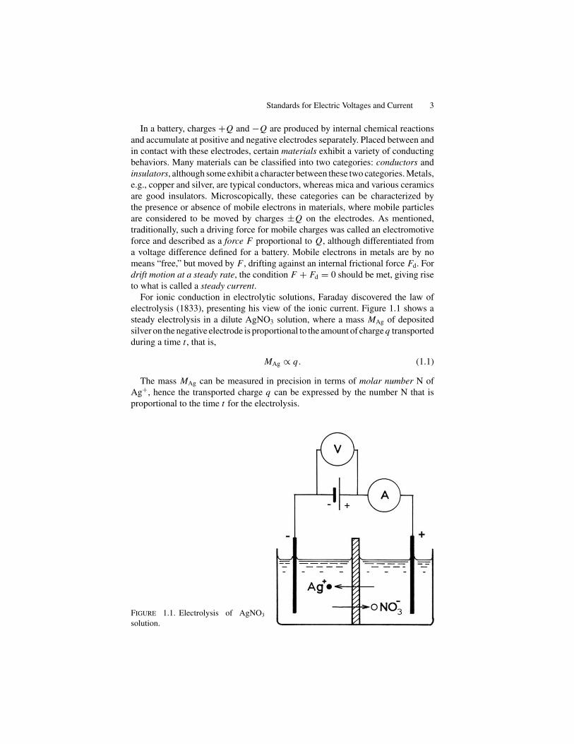
For ionic conduction in electrolytic solutions, Faraday discovered the law ofelectrolysis (1833), presenting his view of the ionic current. Figure 1.1 shows asteady electrolysis in a dilute AgNO3 solution, where a mass MAg of depositedsilver on the negative electrode is proportional to the amount of charge q transportedduring a time t , that is,

MAg ∝ q. (1.1)

The mass MAg can be measured in precision in terms of molar number N ofAg+, hence the transported charge q can be expressed by the number N that isproportional to the time t for the electrolysis.

FIGURE 1.1. Electrolysis of AgNO3

solution.


With accurately measured MAg and t , the current I = q/t can be determinedin great precision. Using an electrolytic cell, a current that deposits 1.1180 mg ofsilver per second is defined as one ampere (1A). Referring to the current of 1A,the unit for a charge is called 1 coulomb, i.e., 1C = 1A-sec.

To move a charge q through a connecting wire, the battery must supply an energyW that should be proportional to q, and therefore we define the quantity V = W/q,called the potential or electric potential. The MKS unit for W is J, so that the unitof V can be specified by J-C−1, which is called a “volt” and abbreviated as V.

In the MKS unit system the ampere (A) for a current is a fundamental unit,whereas “volt” is a derived unit from ampere. Including A as an additional basicunit, the unit system is referred to as the “MKSA system.” Nevertheless, a cadmiumcell, for example, provides an excellent voltage standard: Vemf = 1.9186 × 0.0010V with excellent stability 1�V/yr under ambient conditions.

A practical passage of a current is called a circuit, connecting a battery andanother device with conducting wires. For a steady current that is time-independent,we consider that each point along a circuit can be uniquely specified by an electricpotential, and a potential difference between two points is called voltage. Thepotential V is a function of a point x along the circuit, and the potential differenceV (+) − V (−) between terminals + and − of a battery is equal to the emf voltage,Vemf. If batteries are removed from a circuit, there is, naturally, no current; thepotentials are equal at all points in the circuit—that is, V (x) = const in the absenceof currents.

1.3. Ohm Law’s and Heat Energy

Electric conduction takes place through conducting materials, constituting a majorsubject for discussion in solid state physics. In the classical description we consideronly idealized conductors, either metallic or electrolytic. In the former electrons arecharge carriers, whereas in the latter both positive and negative ions are mobile,contributing to the electrolytic current. These carriers can drift in two oppositedirections; however, the current is defined for expressing the amount of charges|Q| transported per unit time, which is basically a scalar quantity, as will beexplained in the following discussion. In this context how to specify the currentdirection is a matter of convenience. Normally, the current is considered to flowin the direction for decreasing voltage, namely from a higher to a lower voltage.

Because it is invisible the current is “seen” by three major effects, of whichmagnetic and chemical effects have already been discussed. The third effect is heatproduced by currents in a conducting passage, for which Ohm (1826) discoveredthe basic law of electrical resistance. Joule (ca. 1845) showed later that heatproduced by a current is nothing but dissipated energy in a conductor.

Consider a long conducting wire of a uniform cross-sectional area S. Figure 1.2illustrates a steady flow of electrons through a cylindrical passage, where weconsider a short cylindrical volume S�x between x − �x and x along the wire.

Ohm Law’s and Heat Energy 5

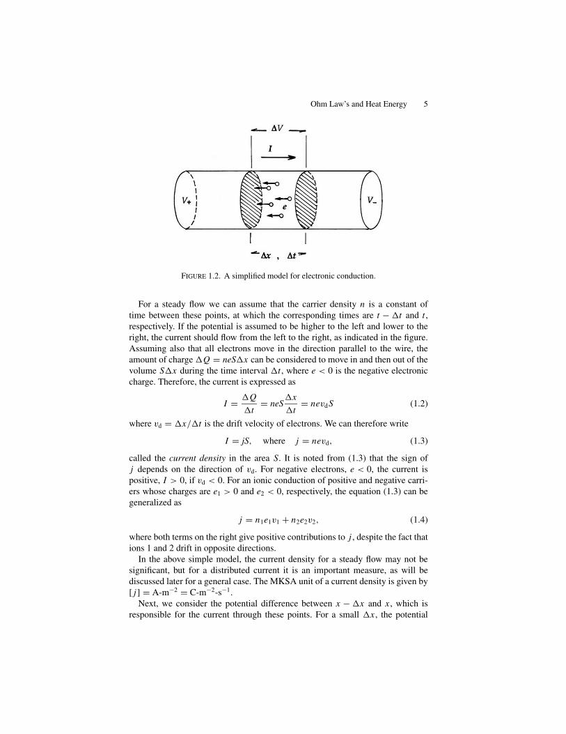
FIGURE 1.2. A simplified model for electronic conduction.

For a steady flow we can assume that the carrier density n is a constant oftime between these points, at which the corresponding times are t − �t and t ,respectively. If the potential is assumed to be higher to the left and lower to theright, the current should flow from the left to the right, as indicated in the figure.Assuming also that all electrons move in the direction parallel to the wire, theamount of charge �Q = neS�x can be considered to move in and then out of thevolume S�x during the time interval �t , where e < 0 is the negative electroniccharge. Therefore, the current is expressed as

I = �Q

�t= neS

�x

�t= nevdS (1.2)

where vd = �x/�t is the drift velocity of electrons. We can therefore write

I = jS, where j = nevd, (1.3)

called the current density in the area S. It is noted from (1.3) that the sign ofj depends on the direction of vd. For negative electrons, e < 0, the current ispositive, I > 0, if vd < 0. For an ionic conduction of positive and negative carri-ers whose charges are e1 > 0 and e2 < 0, respectively, the equation (1.3) can begeneralized as

j = n1e1v1 + n2e2v2, (1.4)

where both terms on the right give positive contributions to j , despite the fact thations 1 and 2 drift in opposite directions.

In the above simple model, the current density for a steady flow may not besignificant, but for a distributed current it is an important measure, as will bediscussed later for a general case. The MKSA unit of a current density is given by[ j] = A-m−2 = C-m−2-s−1.

Next, we consider the potential difference between x − �x and x , which isresponsible for the current through these points. For a small �x , the potential


difference �V can be calculated as

�V = V (x − �x) − V (x) = −F�x,

where the quantity F = −�V/�x represents the driving force for a hypotheticalunit charge 1C. Nevertheless, there is inevitably a frictional force in the conductingmaterial, as can be described by Hooke’s law in mechanics, expressed by Fd =−kvd, where k is an elastic constant.

For a steady current, we have F = −Fd, and therefore we can write

�V = Fd�x = kv d�x .

Eliminating vd from this expression and (1.2), we obtain

�V = �RI, where �R =(

k

neS

)�x,

the electrical resistance between x − �x and x . For a uniform wire, this resultcan be integrated to obtain the total resistance from the relation, that is,

−∫ B

A

dV = V (A) − V (B) = Vemf = I k

neS

∫ L

0

dx = RI ,

where

R = kL

neS= �

L

S(1.5)

is the resistance formula for a uniform conductor that can be calculated as the

length L and cross-sectional area S are specified. The constant � = k

neis called the

resistivity, and its reciprocal 1/� = � is the conductivity of the material. Writinga potential difference and resistance between two arbitrary points as �V and R,Ohm’s law can be expressed as

�V = RI . (1.6)

Obviously, the current occurs if there is a potential difference in a circuit. Thatis, if no current is present the conductor is static and characterized by a constantpotential at all points. Values of � listed in Tables 1.1 and 1.2 are for representativeindustrial materials useful for calculating resistances.

The current loses its energy when flowing through a conducting material, asevidenced by the produced heat. Therefore, to maintain a steady current, the con-nected battery should keep producing charges at the expense of stored energy inthe battery. Although obvious by what we know today, the energy relation for heatgeneration was first verified by Joule (ca. 1845), who demonstrated equivalenceof heat and energy.

Figure 1.3 shows Joule’s experimental setup. To flow a current I through theresistor R, a battery of Vemf performs work. The work to drive a charge �Q outof the battery is expressed by �W = Vemf�Q, and hence we can write �W =(RI)�Q, using Ohm’s law.

Ohm Law’s and Heat Energy 7

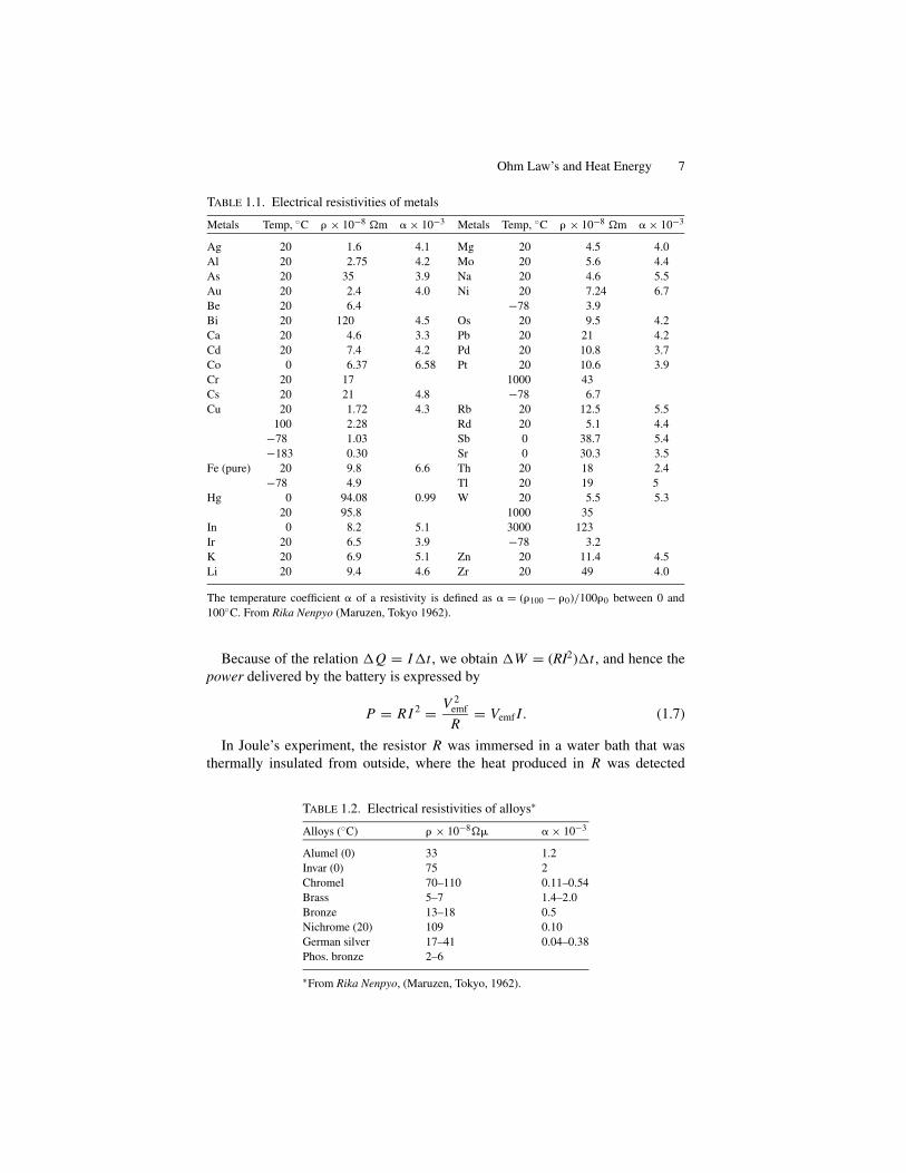
TABLE 1.1. Electrical resistivities of metals

Metals Temp, ◦C � × 10−8 �m � × 10−3 Metals Temp, ◦C � × 10−8 �m � × 10−3

Ag 20 1.6 4.1 Mg 20 4.5 4.0

Al 20 2.75 4.2 Mo 20 5.6 4.4

As 20 35 3.9 Na 20 4.6 5.5

Au 20 2.4 4.0 Ni 20 7.24 6.7

Be 20 6.4 −78 3.9

Bi 20 120 4.5 Os 20 9.5 4.2

Ca 20 4.6 3.3 Pb 20 21 4.2

Cd 20 7.4 4.2 Pd 20 10.8 3.7

Co 0 6.37 6.58 Pt 20 10.6 3.9

Cr 20 17 1000 43

Cs 20 21 4.8 −78 6.7

Cu 20 1.72 4.3 Rb 20 12.5 5.5

100 2.28 Rd 20 5.1 4.4

−78 1.03 Sb 0 38.7 5.4

−183 0.30 Sr 0 30.3 3.5

Fe (pure) 20 9.8 6.6 Th 20 18 2.4

−78 4.9 Tl 20 19 5

Hg 0 94.08 0.99 W 20 5.5 5.3

20 95.8 1000 35

In 0 8.2 5.1 3000 123

Ir 20 6.5 3.9 −78 3.2

K 20 6.9 5.1 Zn 20 11.4 4.5

Li 20 9.4 4.6 Zr 20 49 4.0

The temperature coefficient � of a resistivity is defined as � = (�100 − �0)/100�0 between 0 and

100◦C. From Rika Nenpyo (Maruzen, Tokyo 1962).

Because of the relation �Q = I�t , we obtain �W = (RI2)�t , and hence thepower delivered by the battery is expressed by

P = RI 2 = V 2emf

R= Vemf I. (1.7)

In Joule’s experiment, the resistor R was immersed in a water bath that wasthermally insulated from outside, where the heat produced in R was detected

TABLE 1.2. Electrical resistivities of alloys∗

Alloys (◦C) � × 10−8�� × 10−3

Alumel (0) 33 1.2

Invar (0) 75 2

Chromel 70–110 0.11–0.54

Brass 5–7 1.4–2.0

Bronze 13–18 0.5

Nichrome (20) 109 0.10

German silver 17–41 0.04–0.38

Phos. bronze 2–6

∗From Rika Nenpyo, (Maruzen, Tokyo, 1962).


FIGURE 1.3. A set-up for Joule’s experiment.

by the thermometer immersed in the water. Joule showed that the energy deliv-ered by the battery, i.e., �W = P�t , was equal to the product C��, where Cis the heat capacity of water bath, and ��. the observed temperature rise. From(1.7), the unit of power—the watt (W)—is given by the electrical units of volt× ampere, making the MKSA system more practical than the traditional CGSsystem.

Owing to Joule’s experiment, a traditional unit for heat—“calorie” (cal)—is nolonger necessary, replaced by “joule”(J) although “calorie” and “kilocalorie” arestill familiar units in biological and chemical sciences. The conversion between Jand cal can be made by the relation 1 cal = 4.184 J. With the Ohm law, the MKSAunit of a resistance R is V-A−1, which is called “ohm”, and expressed as �

1.4. The Kirchhoff Theorem

In an electric circuit, a battery is a current source in conducting resistors, providingdistributed potentials V (x) along the circuit. In a simple circuit where a battery ofVemf is connected with one resistor R, the Ohm law Vemf = RI can be interpreted

The Kirchhoff Theorem 9

to mean that the current I circulates in the direction from the positive terminal tothe negative terminal along a closed loop circuit of Vemf and R. In this descriptionthe current direction inside the battery is opposite to the current direction in theresistance; however such a contradiction can be disregarded if we consider thatthe mechanism inside the battery is not our primary concern. Kirchhoff (1849)extended such an interpretation to more general circuits consisting of many emf’sand resistors, and formulated the general theorem to deal with currents throughthese resistors.

In a steady-current condition, we consider that the potential V (x) is signified bya unique value at any point x along the current passage, whereas at specific pointsxi where batteries are installed, we consider discontinuous voltages Vemf(xi). Asteady current Ij can flow through each resistor Rj that are indexed j = 1, 2, . . . ,

but the current direction and the potential difference across Rj can be left asprimarily unknown. Also in a circuit are junctions in the current passage, indexedby k = 1, 2, . . . , where more than two currents are mixed.

For a general circuit, we can consider several closed loops, �, �, . . . , which canbe either part of the circuit or can make up the whole circuit. It is significant thatV (x) takes a unique value at any given point x , so that the potential value shouldbe the same, no matter how the current circulates along a closed loop in eitherdirection. Mathematically, this can be expressed by

∮C dV = 0 along any of these

loops C of a given circuit, for which we can write∑i

Vemf (xi) =∑

j

Rj Ij. (1.8)

Known as the Kirchhoff theorem, (1.8) can be applied to any closed loop inthe circuit. Next, at any junction k of steady currents, we note that total incomingcurrents must be equal to total outgoing currents, namely, there is no accumulatedcharge at the point k; that is the law of current continuity. Assuming all directionsof currents exist arbitrarily at the junction, we must have the relation∑

k

Ik = 0 (1.9)

at all junctions, which is known as Kirchhoff’s junction theorem. As these currentsare primarily unknown, we can usually assume their directions for solving equa-tions (1.8) and (1.9); the assumed current directions are then corrected by signs ofthe solutions.

We solve (1.8) and (1.9) as a set of algebraic equations for unknown currentsIj, j = 1, 2, . . . . However, all of these equations are not required, and hence wecan select equations to solve sufficiently for the given number j of Rj, as shown bythe following examples.

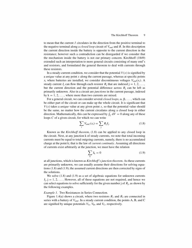
Example 1. Two Resistances in Series Connection.Figure 1.4(a) shows a circuit, where two resistors R1 and R2 are connected in

series with a battery of Vemf. In a steady current condition, the points A, B, and Care signified by unique potentials VA, VB, and VC, respectively.


FIGURE 1.4. (a) Resistances R1 and R2

in series, and (b) in parallel.

Referring to the junction theorem (1.9), we see that for these currents in thefigure we have I1 = I2 = I , representing the “total” current. Accordingly, usingthe Ohm law, we can write

VA − VB = R1 I and VB − VC = R2 I,

hence

VA − VC = (VA − VB) + (VB − VC) = (R1 + R2)I = Vemf,

which expresses Ohm’s law for total resistance R = R1 + R2.

Example 2. Two Resistances in Parallel Connection.Figure 1.4b shows a parallel connection of two resistances R1 and R2. The

junctions A and B are characterized by potentials VA and VB under a steady currentcondition. In this case, I1 and I2 are generally different, but related to the currentI from the battery by the junction theorem (1.9). That is,

I = I1 + I2

at both A and B.For loops �. and �. that include (Vemf, R1) and (Vemf, R2), respectively, we obtain

from (1.8) that

VA − VB = Vemf = R1 I1 = R2 I2.

The Kirchhoff Theorem 11

FIGURE 1.5. Kirchhoff’s theorems. Junctions A and B, loops ABC, ADB, and CDB are

named �, �, and � , respectively.

Solving these equations for I1 and I2, we obtain

I =(

1

R1

+ 1

R2

)Vemf,

and the total resistance R in parallel connections can be determined from

1

R= 1

R1

+ 1

R2

.

Example 3. Calculation of currents in a circuit shown in Figure 1.5. In this cir-cuit, three loops �, �, and � and two junctions A and B can be consideredfor Kirchhoff’s theorem, as shown in the figure; however, we only need threeequations to solve (1.8) and (1.9) for I1, I2, and I3. Also, to set up three equa-tions, the directions of currents can be assumed arbitrarily, as indicated in thefigure.

Here, we apply (1.8) to the loops �, and �, and (1.9) to the junction A. Referringto assigned current directions, we can write three equations, respectively, for �, �,and A, which are

I1 R1 + (−I2)R2 + Va = 0,

(−I1)R1 + (−I3)R3 + (−Vb) = 0,


and

I1 + I2 + (−I3) = 0.

Solving these equations, we obtain

I1 = − Vb R2 − Va R3

R1 R2 + R2 R3 + R3 R1

,

I2 = − (Va − Vb) R1 + Vb R3

R1 R2 + R2 R3 + R3 R1

and

I3 = − (Va − Vb) R1 + Vb R2

R1 R2 + R2 R3 + R3 R1

.

Part 1Electrostatics

13

2Electrostatic Fields

2.1. Static Charges and Their Interactions

In early physics, static electricity was studied as a subject independent from mag-netism; it was after Oersted’s experiment that the relation between an electriccurrent and the magnetic field was recognized. Today, static and dynamic electric-ity are viewed as clearly exclusive phenomena; however, many early findings onstatic phenomena significantly contributed to establishing present day knowledgeof electromagnetism.

First recognized as frictional electricity, static charges were also observed to beproduced chemically from batteries, although static effects were only primitivelymeasured in early experiments. Also recognized early were mobile charges inconducting materials, which were noticed as distributed on surfaces of a pairof metal plates separated by a narrow air gap, in particular, when the plates wereconnected with battery terminals. In early physics, such a device, called a capacitor,was used for studying the nature of static charges. On these plates, charges +Qand −Q appeared to condense from the battery, and hence such a device was oftenreferred to as a condenser. Empirically, it was found that these opposite chargesattract each other across the narrow gap, whereas charges of the same kind on eachplate repel each other, so that such a “condensation” process ceases eventually atfinite ±Q. Such static interactions between charges constitute the empirical rulefor electric quantities, although the origin is still not properly explained by the firstprinciple. In this context, we simply accept the empirical rule as a fact in natureon which the present electromagnetic theory is founded.

It is notable that static charges reside at stationary sites on conducting surfaces inequilibrium with their surroundings. In the static condition, the absence of movingcharges signifies the state of a conductor that is characterized by a constant electricpotential, namely V (x) = const at all points x .

The amount of charge Q that accumulates on condenser plates is proportionalto the voltage Vemf of the battery, depending on the geometrical structure of thedevice. Therefore, we write the relation

Q = CVemf, (2.1)

15

16 2. Electrostatic Fields

FIGURE 2.1. A capacitor Cand a battery Vemf (a) beforeconnection, (b) connected, (c)disconnected after charged.

where the constant C , referred to as capacity, is determined by the device geometry.In equation (2.1), Q represents the maximum charge that is transferred to thecapacitor. The MKSA unit for the capacity is C-V−1, which is called farad (F).

Figure 2.1 illustrates a capacitor of two parallel metal plates facing across anarrow gap, which is connected with a battery as shown. Such a capacitor is astandard device for electrostatics and discussed as a theoretical model as well.Figures 2.1(a) and (b) show a parallel-plate capacitor and a battery before andafter connection, respectively. The empty capacitor (Figure 2.1(a)) can be chargedby the battery (Figure 2.1(b)). Figure 2.1(c) shows the charged capacitor discon-nected from the battery. Figures 2.1(b) and (c) show the space between the platesis signified by an electric field E that is related to charges on the plates. It is sig-nificant that the charges and field remain in the capacitor even after the batteryis removed, as seen in the attractive force that exists between the plates acrossthe gap.

Interactions among carrier particles are responsible for a charge distributionin the capacitor, resulting in a significant attraction between plates of oppositecharge, whereas like charges are distributed at uniform densities on surface areasthat face each other. Hence, the charged capacitor should be characterized by apotential energy due to an attractive force between the plates on which the batteryperformed work to transport ±Q.

2.2. A Transient Current and Static Charges

When a capacitor is connected with a battery, charges are transported in the circuituntil the circuit reaches a steady state. Accordingly, the charging rate dQ/dt , calleda transient current, flows during the charging process. Such a current depends onthe resistance R of wire connecting the capacitor with the battery, as shown inFigure 2.2.

A Transient Current and Static Charges 17

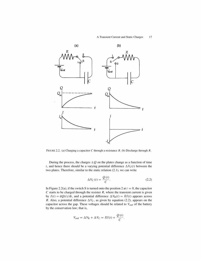
FIGURE 2.2. (a) Charging a capacitor C through a resistance R. (b) Discharge through R.

During the process, the charges ±Q on the plates change as a function of timet , and hence there should be a varying potential difference �VC(t) between thetwo plates. Therefore, similar to the static relation (2.1), we can write

�VC (t) = Q (t)

C. (2.2)

In Figure 2.2(a), if the switch S is turned onto the position 2 at t = 0, the capacitorC starts to be charged through the resister R, where the transient current is givenby I (t) = dQ(t)/dt , and a potential difference �VR(t) = RI (t) appears acrossR. Also, a potential difference �VC , as given by equation (2.2), appears on thecapacitor across the gap. These voltages should be related to Vemf of the batteryby the conservation law; that is,

Vemf = �VR + �VC = RI (t) + Q (t)

C.


Multiplying both sides by I (t), the power delivered by the battery can be calculatedas

P(t) = Vemf I (t) = RI (t)2 + Q (t)

C

dQ (t)

dt.

Hence, we can obtain the energy W (t) spent by the battery between t = 0 and alater time t by integrating P(t); i.e.,

W (t) = R∫ t

0I (t)2 dt + 1

2CQ (t)2 .

The first term on the right represents heat dissipated in R, and the second one isthe energy stored in the capacitor during the time t .

To obtain the transient current, we solve the following differential equation,assuming that Vemf is a constant of time. Namely,

RdQ (t)

dt+ Q (t)

C= const, (2.2a)

or

RdI (t)

dt+ I (t)

C= 0 (2.2b)

with a given initial condition. In the circuit shown in Figure 2.2(a), when the switchS is turned to position 1, a steady current Io determined by Vemf = RI o is flowinginitially through R. In this case, when S is turned on to 2 at t = 0, charging beginsto take place in the capacitor C . On the other hand, equation 2.2(b) shows a casewhere a charged capacitor C starts discharging at t = 0, after the switch S is turnedto the position 2.

In the latter case, equation (2.2b) can be integrated with the initial conditionI = Io at t = 0, resulting in the transient current expressed by

I (t) = Io exp(− t

RC), (2.3a)

showing an exponential decay. In this case, the charge Q(t) on the capacitor platecan be expressed by

Q(t) =∫ t

0I (t) dt = I0 RC exp

(− t

RC

)∣∣∣∣t

0

= Qmax

[1 − exp

(− t

RC

)], (2.3b)

where Qmax = Io RC is the maximum amount of charge reached as t → ∞. We canalso solve equation (2.2b) with the initial condition Q = Qmax at t = 0 to obtainsimilar expressions to discharging the capacitor C . In Figure 2.3, the transientcharge and current given by equations (2.3a) and (2.3b) and similar transients fordischarging are shown below circuit diagrams. For these transient currents, it isnoted that the parameter defined by � = 1/RC represents a characteristic time ofthe transient current, and hence is called the time constant. For R = 100 k� andC = 0.1 �F, for example, the time constant is � = 10−2s, giving the “timescale”of the transient phenomena in the RC circuit. Figure 2.3 illustrates a modernized

Uniform Electric Field in a Parallel-Plate Condenser 19

FIGURE 2.3. Transient voltages �VR and �VC observed by a cathode-ray oscilloscope(CRO).

circuit using a cathode-ray oscilloscope (CRO) for demonstrating such transientson the screen.

In the above argument, when a capacitor is charged to ±Q, a potential difference�V appears across the plates, between which an energy Q2/2C = 1

2 C(�V )2

should be stored. A capacity signified by the variables Q and �V indicates thatthere is an electric field in the space between the plates.

2.3. Uniform Electric Field in a Parallel-Plate Condenser

In a charged condenser, the plates attract each other across the gap, originatingfrom electrostatic forces between +Q and −Q, as implied by the Coulomb law(1785) for point charges. It was postulated in early physics that such a force prop-agates through the empty space, called the field; this idea was, however, not easilyaccepted unless it was duly verified. Nevertheless, Faraday (ca. 1850) describedsuch a field with line drawings, which led Maxwell (1873) to establish his math-ematical theory of electromagnetic fields. Today, supported by much evidence,the electromagnetic field is a well-established concept, one that represents a realphysical object. Therefore, we can define a static electric field as implemented byFaraday and Maxwell.

2.3.1. The Electric Field Vector

In a charged parallel-plate capacitor signified by the potential difference �V acrossthe empty gap, we can consider a potential function V (z) for the field in the emptyspace, where z is a position on a straight line perpendicular to the plates. Theconducting plate surfaces of a large area are signified by constant voltages VA andVB, so that the potential in the uniform field can be expressed as

V (r, z) = −Ez + const, (2.4a)


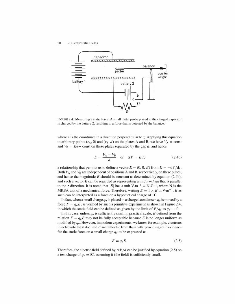
FIGURE 2.4. Measuring a static force. A small metal probe placed in the charged capacitoris charged by the battery 2, resulting in a force that is detected by the balance.

where r is the coordinate in a direction perpendicular to z. Applying this equationto arbitrary points (rA, 0) and (rB, d) on the plates A and B, we have VA = constand VB = Ed+ const on these plates separated by the gap d, and hence

E = VA − VB

dor �V = Ed, (2.4b)

a relationship that permits us to define a vector E = (0, 0, E) from E = −dV/dz.Both VA and VB are independent of positions A and B, respectively, on these plates,and hence the magnitude E should be constant as determined by equation (2.4b),and such a vector E can be regarded as representing a uniform field that is parallelto the z direction. It is noted that |E| has a unit V-m−1 = N-C−1, where N is theMKSA unit of a mechanical force. Therefore, writing E = 1 × E in V-m−1, E assuch can be interpreted as a force on a hypothetical charge of 1C.

In fact, when a small charge qo is placed in a charged condenser, qo is moved by aforce F = qo E , as verified by such a primitive experiment as shown in Figure 2.4,in which the static field can be defined as given by the limit of F/qo as qo → 0.

In this case, unless qo is sufficiently small in practical scale, E defined from therelation F = qo E may not be fully acceptable because E is no longer uniform asmodified by qo. However, in modern experiments, we know, for example, electronsinjected into the static field E are deflected from their path, providing solid evidencefor the static force on a small charge qo to be expressed as

F = qo E . (2.5)

Therefore, the electric field defined by �V/d can be justified by equation (2.5) ona test charge of qo =1C, assuming it (the field) is sufficiently small.

Uniform Electric Field in a Parallel-Plate Condenser 21

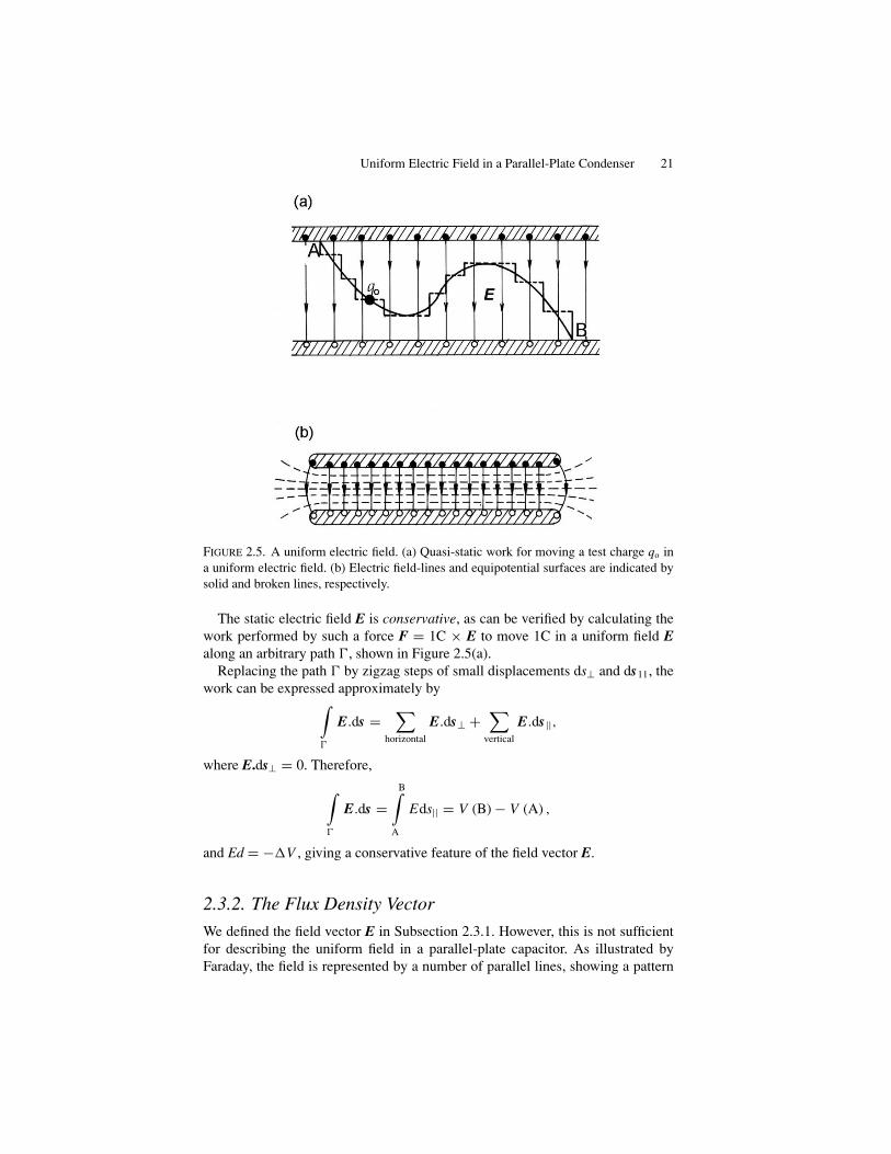
FIGURE 2.5. A uniform electric field. (a) Quasi-static work for moving a test charge qo ina uniform electric field. (b) Electric field-lines and equipotential surfaces are indicated bysolid and broken lines, respectively.

The static electric field E is conservative, as can be verified by calculating thework performed by such a force F = 1C × E to move 1C in a uniform field Ealong an arbitrary path �, shown in Figure 2.5(a).

Replacing the path � by zigzag steps of small displacements ds⊥ and ds11, thework can be expressed approximately by∫

�

E.ds =∑

horizontal

E.ds⊥ +∑

vertical

E.ds||,

where E.ds⊥ = 0. Therefore,

∫�

E.ds =B∫

A

Eds|| = V (B) − V (A) ,

and Ed = −�V , giving a conservative feature of the field vector E.

2.3.2. The Flux Density Vector

We defined the field vector E in Subsection 2.3.1. However, this is not sufficientfor describing the uniform field in a parallel-plate capacitor. As illustrated byFaraday, the field is represented by a number of parallel lines, showing a pattern

Physics of Classical Electromagnetism · The Maxwell theory of electromagnetism was well established in the latter nine-teenth century, when H. R. Hertz demonstrated the electromagnetic

Documents