UMM AL-QURA UNIVERSITY - College of Applied Science- Department of Physics 1 / 34 Physics Laboratory Manual Prepared by Committee of Laboratories General Physics Lab. (102)

Welcome message from author
This document is posted to help you gain knowledge. Please leave a comment to let me know what you think about it! Share it to your friends and learn new things together.
Transcript
UMM AL-QURA UNIVERSITY - College of Applied Science- Department of Physics
1 / 34
Physics
Laboratory Manual Preparedby
CommitteeofLaboratories
General Physics Lab. (102)
UMM AL-QURA UNIVERSITY - College of Applied Science- Department of Physics
2 / 34
Introduction (1): Safety and importance of laboratory work
Objective: By the end of this lesson, the student should know the followings:
I- Safety and Security in the Laboratory.
1. The Name of the supervisor of the Lab.
2. The telephone No.s of the emergency within the faculty and the University and Kingdom of Saudi Arabia.
3. The place of the first aid bag and how to use it
4. The place of Fire-extinguisher and how to use it
5. How to exit the Lab and the building in an emergency
6. How to give the first aid to the others
7. How to protect your eyes
8. How to protect your skin
9. The general instruction of the safety and security
II- Introduction to the Laboratory.
1. Aim of the Experiments
2. The importance of the experimental work
3. General Instructions for Performing Experiments
4. How to Record an Experiment in the Practical File
Aim of the experiments
In Physics, an experiment is an empirical procedure that arbitrates between competing
models or hypotheses. Researchers also use experimentation to test existing theories or
new hypotheses to support or disprove them. Experiments form the foundation of the
growth and development of science. The chief aim of experimentation in science is:
UMM AL-QURA UNIVERSITY - College of Applied Science- Department of Physics
3 / 34
1- Discovering the law which governs a certain phenomenon,
2- Verifying a given law which has been derived from a theory
3- Determination of physical constants
4- Determination of the physical properties
A general scheme of scientific investigation known as the Scientific Method involves
the following steps:
1- Observations: Qualitative information about a phenomenon collected by unaided senses.
2- Experimentation: Quantitative measurements (with the help of instruments) of certain physical quantities which have some bearing on the phenomenon.
3- Formulation of hypothesis: Analysis of the data to determine how various measured quantities affect the phenomenon and to establish a relationship between them, graphically or otherwise.
4- Verification: The hypothesis is verified by applying it to other allied phenomena.
5- Predictions of new phenomena.
6- New experiments to test the predictions.
7- Modification of the law if necessary
The above discussion shows that experimentation is vital to the development of any
kind of science and more so to that of Physics.
Importance of Laboratory work
Physics is an experimental science and the history of science reveals the fact that most
of the notable discoveries in science have been made in the laboratory. Seeing
experiments being performed, i.e., demonstration experiments are important for
understanding the principles of science. However, performing experiments by one’s
own hands is far more important because it involves learning by doing. It is needless to
emphasize that for a systematic and scientific training of a young mind; a genuine
laboratory practice is a must.
General Instructions for performing experiments

UMM AL-QURA UNIVERSITY - College of Applied Science- Department of Physics
4 / 34
1. Before performing an experiment, the student should first thoroughly understand the
theory of the experiment. The objectives of the experiment, the type of apparatus
needed and the procedure to be followed should be clear before actually performing
the experiment. The difficulties and doubts if any, should be discussed with the
supervisor.
2. The student should check up whether the right type of apparatus for the experiment
to be performed is given to him or not.
3. All the apparatus should be arranged on the table in proper order. Every apparatus
should be handled carefully and cautiously to avoid any damage. Any damage or
breaking done to the apparatus accidentally, should be immediately brought to the
notice.
4. Precautions meant for the experiment should not only be read and written in the
practical file, but they are to be actually observed while doing the experiment.
5. All observations should be taken systematically, intelligently and should be honestly
recorded on the fair record book. In no case an attempt should be made to cook or
change the observations in order to get good results.
6. Repeat every observation, number of times even though their values each time may
be exactly the same. The student must bear in mind the proper plan for recording the
observations.
7. Calculations should be neatly shown using log tables. The degree of accuracy of the
measurement of each quantity should always be kept in mind so that the final result
does not show any fictitious accuracy. So the result obtained should be suitably
rounded off.
8. Wherever possible, the observations should be represented with the help of graph.
9. Always mention the proper unit with the result.
UMM AL-QURA UNIVERSITY - College of Applied Science- Department of Physics
5 / 34
Introduction (2): General Instruction
Objective: This lesson is an introduction to the experimental work. By the end of this
lesson, the student should know the followings :
1. Error and Observations
2. Accuracy of Observations
3. Accuracy of the Result
4. Permissible Error in the Result
5. How to Estimate the Permissible Error in the Result
6. Estimating Maximum Permissible Error
7. Percentage Error
8. Significant Figures (Precision of Measurement (
9. Logarithms
10. Graph
11. Calculations of Slope of a Straight Line
12. Rules for Measurements in the Laboratory
13. How to write a Lab report.
1- Errors and Observations
We come across following errors during the course of an experiment:
Personal or chance error: Two observers using the same experimental set up,
do not obtain exactly the same result. Even the observations of a single
experimenter differ when it is repeated several times by him or her. Such errors
always occur inspite of the best and honest efforts on the part of the
experimenter and are known as personal errors. These errors are also called
chance errors as they depend upon chance. The effect of the chance error on the
result can be considerably reduced by taking a large number of observations
and then taking their mean.
UMM AL-QURA UNIVERSITY - College of Applied Science- Department of Physics
6 / 34
Error due to external causes: These are the errors which arise due to reasons
beyond the control of the experimenter, e.g., change in room temperature,
atmospheric pressure etc. A suitable correction can however, be applied for
these errors if the factors affecting the result are also recorded.
Instrumental errors: Every instrument, however cautiously designed or
manufactured, possesses imperfection to some extent. As a result of this
imperfection, the measurements with the instrument cannot be free from errors.
Errors, however small, do occur owing to the inherent manufacturing defects in
the measuring instruments. Such errors which arise owing to inherent
manufacturing defects in the measuring instruments are called instrumental errors. These errors are of constant magnitude and suitable corrections can be
applied for these errors.
2- Accuracy of Observations
The manner, in which an observation is recorded, indicates how accurately the physical
quantity has been measured. For example, if a measured quantity is recorded as 50 cm,
it implies that it has been measured correct ‘to the nearest cm’. It means that the
measuring instrument employed for the purpose has the least count (L.C.) = 1 cm .
Since the error in the measured quantity is half of the L.C. of the measuring
instrument, therefore, here the error is 0.5 cm in 50 cm. In other words we can say, the
error is 1 part in 100.
If the observation is recorded in another way, i.e., 50.0 cm, it implies that it is correct
‘to the nearest mm. As explained above, the error now becomes 0.5 mm or 0.05 cm in
50 cm. So the error is 1 part in 1000.
If the same observation is recorded as 50.00 cm. It implies that reading has been taken
with an instrument whose L.C. is 0.01 cm. Hence the error here becomes 0.005 cm in
50 cm, i.e., 1 part in 10,000.
It may be noted that with the decrease in the L.C. of the measuring instrument, the
error in measurement decreases, in other word accuracy of measurement increases.
When we say the error in the measurement of a quantity is 1 part in 1000, we can also
say that the accuracy of the measurement is 1 part in 1000. Both the statements mean
the same thing. Thus, from the above discussion it follows that:
UMM AL-QURA UNIVERSITY - College of Applied Science- Department of Physics
7 / 34
a) The accuracy of measurement increases with the decrease in the least count of the
measuring instrument; and
b) The manner of recording an observation indicates the accuracy of its measurement
3- Accuracy of the Result
The accuracy of the final result is always governed by the accuracy of the least
accurate observation involved in the experiment. So after making a calculation, the
result should be expressed in such a manner that it does not show any superfluous
accuracy. Actually the result should be expressed up to that decimal place (after
rounding off) which indicates the same accuracy of measurement as that of the least
accurate observation made.
4- Permissible error in the Result Even under ideal conditions in which personal errors, instrumental errors and errors
due to external causes are some how absent, there is another type of error which creeps
into the Introductory observations because of the limitation put on the accuracy of the
measuring instruments by their least counts. This error is known as the permissible
error.
5- How to estimate the permissible error in the result
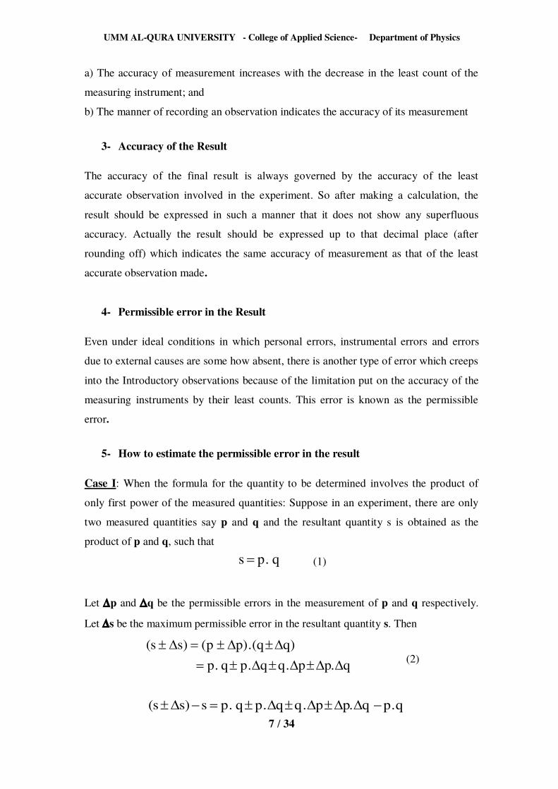
Case I: When the formula for the quantity to be determined involves the product of
only first power of the measured quantities: Suppose in an experiment, there are only
two measured quantities say p and q and the resultant quantity s is obtained as the
product of p and q, such that q.ps (1)
Let p and q be the permissible errors in the measurement of p and q respectively.
Let s be the maximum permissible error in the resultant quantity s. Then
q.pp.qq.pq.p)qq(.)pp()ss(
(2)
q.pq.pp.qq.pq.ps)ss(
UMM AL-QURA UNIVERSITY - College of Applied Science- Department of Physics
8 / 34
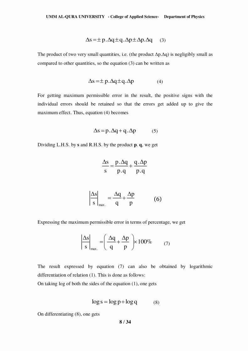
q.pp.qq.ps (3)
The product of two very small quantities, i.e. (the product p.q) is negligibly small as
compared to other quantities, so the equation (3) can be written as
p.qq.ps (4)
For getting maximum permissible error in the result, the positive signs with the
individual errors should be retained so that the errors get added up to give the
maximum effect. Thus, equation (4) becomes
p.qq.ps (5)
Dividing L.H.S. by s and R.H.S. by the product p. q, we get
q.pp.q
q.pq.p
ss
pp
ss
.max
(6)
Expressing the maximum permissible error in terms of percentage, we get
%100pp
ss
.max
(7)
The result expressed by equation (7) can also be obtained by logarithmic
differentiation of relation (1). This is done as follows:
On taking log of both the sides of the equation (1), one gets
qlogplogslog (8)
On differentiating (8), one gets
UMM AL-QURA UNIVERSITY - College of Applied Science- Department of Physics
9 / 34
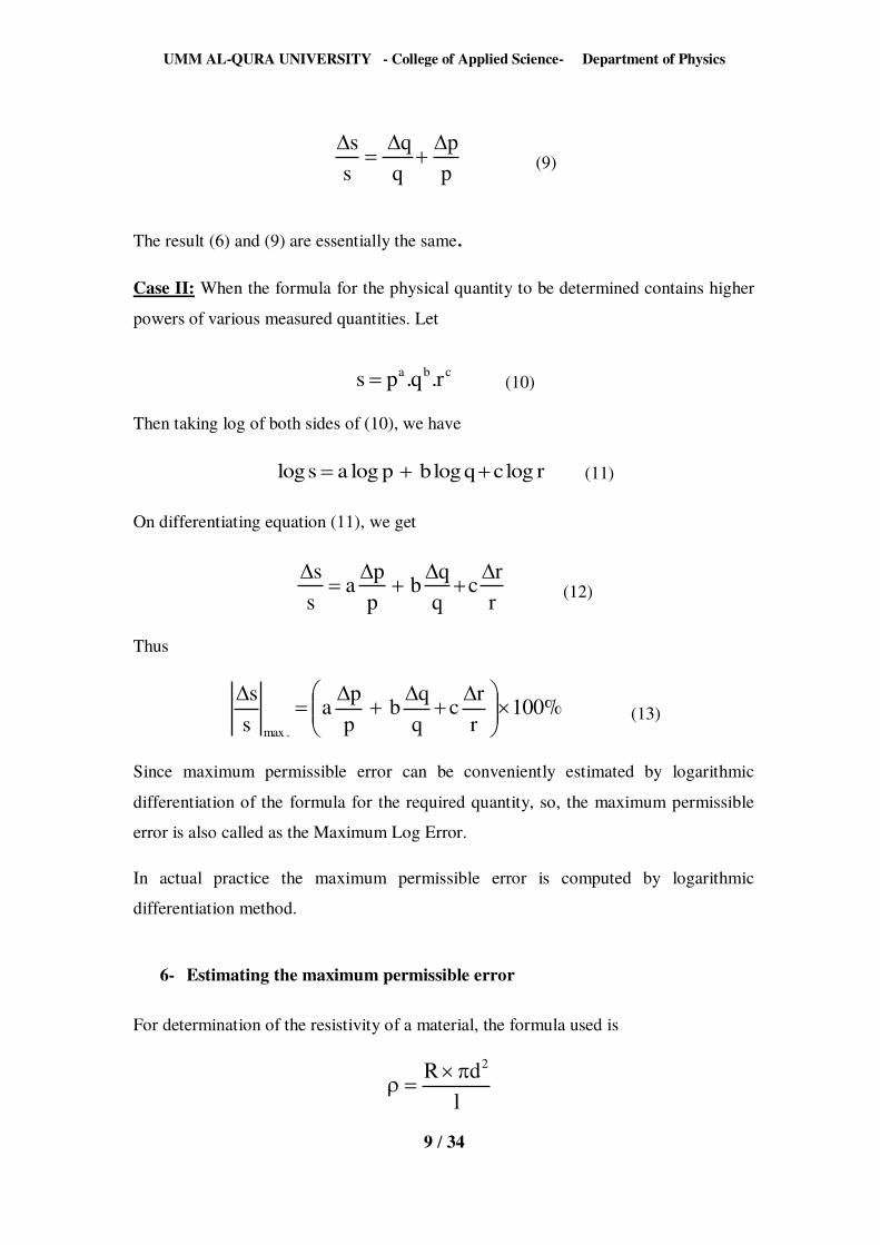
pp
ss
(9)
The result (6) and (9) are essentially the same.
Case II: When the formula for the physical quantity to be determined contains higher
powers of various measured quantities. Let
cba r.q.ps (10)
Then taking log of both sides of (10), we have
rlogcqlogbplogaslog (11)
On differentiating equation (11), we get
rrc
qqb
ppa
ss
(12)
Thus
%100rrc
qqb
ppa
ss
.max
(13)
Since maximum permissible error can be conveniently estimated by logarithmic
differentiation of the formula for the required quantity, so, the maximum permissible
error is also called as the Maximum Log Error.
In actual practice the maximum permissible error is computed by logarithmic
differentiation method.
6- Estimating the maximum permissible error
For determination of the resistivity of a material, the formula used is
ldR 2
UMM AL-QURA UNIVERSITY - College of Applied Science- Department of Physics
10 / 34
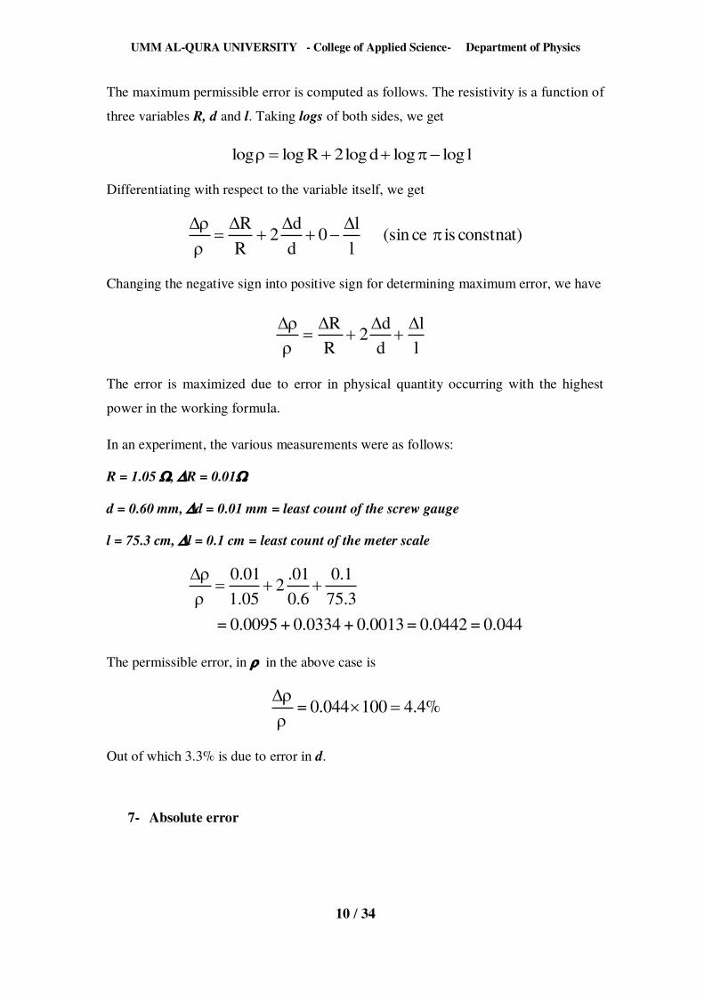
The maximum permissible error is computed as follows. The resistivity is a function of
three variables R, d and l. Taking logs of both sides, we get
lloglogdlog2Rloglog
Differentiating with respect to the variable itself, we get
)constnatisce(sinll0
dd2
RR
Changing the negative sign into positive sign for determining maximum error, we have
ll
dd2
RR
The error is maximized due to error in physical quantity occurring with the highest
power in the working formula.
In an experiment, the various measurements were as follows:
R = 1.05 , R = 0.01
d = 0.60 mm, d = 0.01 mm = least count of the screw gauge
l = 75.3 cm, l = 0.1 cm = least count of the meter scale
0.044 = 0.0442 = 0.0013 + 0.0334 + 0.0095 =3.751.0
6.001.2
05.101.0
The permissible error, in in the above case is
4.4%1000.044 =
Out of which 3.3% is due to error in d.
7- Absolute error
UMM AL-QURA UNIVERSITY - College of Applied Science- Department of Physics
11 / 34
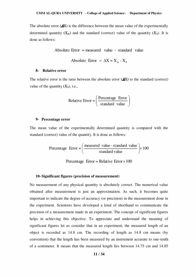
The absolute error (X) is the difference between the mean value of the experimentally
determined quantity (Xm) and the standard (correct) value of the quantity (XS). It is
done as follows:
value standard - valuemeasured=Error Absolute
Sm X - X=XErrorAbsolute
8- Relative error
The relative error is the ratio between the absolute error (X) to the standard (correct)
value of the quantity (XS), i.e.,
valuestandard
Error Percentage=Error Relative
9- Percentage error
The mean value of the experimentally determined quantity is compared with the
standard (correct) value of the quantity. It is done as follows:
100 valuestandard
valuestandard - valuemeasured=Error Percentage
100ErrorRelative=Error Percentage
10- Significant figures (precision of measurement)
No measurement of any physical quantity is absolutely correct. The numerical value
obtained after measurement is just an approximation. As such, it becomes quite
important to indicate the degree of accuracy (or precision) in the measurement done in
the experiment. Scientists have developed a kind of shorthand to communicate the
precision of a measurement made in an experiment. The concept of significant figures
helps in achieving this objective. To appreciate and understand the meaning of
significant figures let us consider that in an experiment, the measured length of an
object is recorded as 14.8 cm. The recording of length as 14.8 cm means (by
convention) that the length has been measured by an instrument accurate to one-tenth
of a centimeter. It means that the measured length lies between 14.75 cm and 14.85
UMM AL-QURA UNIVERSITY - College of Applied Science- Department of Physics
12 / 34
cm. It also indicates that in this way recording of lengths as 14.8 cm, the figures 1 and
4 are absolutely correct whereas the figures ‘8’ is reasonably correct. So in this way of
recording a reading of a measurement, there are three significant figures. Let us now
consider another way of recording a reading. Let the measured length be written as
14.83 cm. This way of writing the value of a length, means that the measurement is
done with an instrument which is accurate up to one-hundredth of a centimeter. It
means that the length lies between 14.835 cm and 14.825 cm, which shows that in
14.83 cm, the figures 1, 4 and 8 are absolutely correct and the fourth figure ‘3’ is only
reasonably correct. Thus, this way of recording length as 14.83 cm contains four
significant figures. Thus, this significant figure is a measured quantity to indicate the
number of digits in which we have confidence. In the above measurement of length,
the first measurement (14.8 cm) is good to three significant figures, whereas the second
one (14.83 cm) is good to four significant figures. From the above discussion, we
should clearly understand that the two ways of recording an observation such as 15.8
cm and 15.80 cm represent two different degrees of precision of measurements.
ROUNDING OFF
When the quantities with different degrees of precision are to be added or subtracted,
then the quantities should be rounded off in such a way that all of them are accurate up
to the same place of decimal. For rounding off the numerical values of various
quantities, the following points are noted.
1. When the digit to be dropped is more than 5, then the next digit to be retained should
be increased by 1.
2. When the digit to be dropped is less than 5, then the next digit should be retained as
it is, without changing it.
3. When the digit to be dropped happens to be the digit 5 itself, then (a) the next digit
to be retained is increased by 1, if the digit is an odd number. (b) the next digit is
retained as it is, if the digit is an even number.
After carrying out the operations of multiplication and division, the final result should
be rounded off in such a manner that its accuracy is the same as that of the least
accurate quantity involved in the operation.
UMM AL-QURA UNIVERSITY - College of Applied Science- Department of Physics
13 / 34
11- Graph
A graph is a pictorial way to show how two physical quantities are related. It is a
numerical device dealing not in cm, ohm, time, temperature, etc. but with the
numerical magnitude of these quantities. Two varying quantities called, the variables
are the essential features of a graph.
Purpose: To show how one quantity varies with the change in the other. The quantity
which is made to change at will, is known as the independent variable and the other
quantity which varies as a result of this change is known as the dependent variable.
The essential features of the experimental observations can be easily seen at a glance if
they are represented by a suitable graph. The graph may be a straight line or a curved
line.
The advantage of Graph: The most important advantage of a graph is that, the average
value of a physical quantity under investigation can be obtained very conveniently
from it without resorting to lengthy numerical computations. Another important
advantage of the graph is that some salient features of a given experimental data can be
seen visually. For example, the points of maxima or minima or inflecion can be easily
known by simply having a careful look at the graph representing the experimental data.
These points cannot so easily be concluded by merely looking at the data. Whenever
possible, the results of an experiment should be presented in a graphical form. As far as
possible, a straight line graph should be used because a straight line is more
conveniently drawn and the deduction from such a graph are more reliable than from a
curved line graph.
Each point on a graph is an actual observation. So it should either be encircled or be
made as an intersection (i.e. cross) of two small lines. The departure of the point from
the graph is a measure of the experimental error in that observation.
How to Plot a Graph? The following points will be found useful for drawing a proper
graph:
1. Examine carefully the experimental data and note the range of variations of the two
variables to be plotted. Also examine the number of divisions available on the two axes
drawn on the graph paper. After doing so, make a suitable choice of scales for the two
UMM AL-QURA UNIVERSITY - College of Applied Science- Department of Physics
14 / 34
axes keeping in mind that the resulting graph should practically cover almost the entire
portion of the graph paper.
2. Write properly chosen scales for the two axes on the top of the graph paper or at
some suitable place. Draw an arrow head along each axis and write the symbol used
for the corresponding variable along with its unit as headings of observations in the
table, namely, d/mm, R/W, l/cm, T/S, I/A etc. Also write the values of the respective
variables on the divisions marked by dark lines along the axes.
3. After plotting the points encircle them. When the points plotted happen to lie almost
on a straight line, the straight line should be drawn using a sharp pencil and a straight
edged ruler and care should be taken to ensure that the straight line passes through the
maximum number of points and the remaining points are almost evenly distributed on
both sides of the line.
4. If the plotted points do not lie on a straight line, draw freehand smooth curve passing
through the maximum number of points. Owing to errors occurring in the observations,
some of the points may not fall exactly on the free hand curve. So while drawing a
smooth curve, care should be exercised to see that such points are more or less evenly
distributed on both sides of the curve.
5. When the plotted points do not appear to lie on a straight line, a smooth curve is
drawn with the help of a device known as French curve. If French curve is not
available, a thin flexible spoke of a broom can also be used for drawing a smooth
curve. To make the spoke uniformly thin throughout its length, it is peeled off suitably
with a knife. This flexible spoke is then held between the two fingers of left hand and
placed on the graph paper bending it suitably with the pressure of the fingers is such a
manner that the spoke in the curved position passes through the maximum number of
points. The remaining points should be more or less evenly distributed on both sides of
the curved spoke. In this bent position of the spoke, a smooth line along the length of
the spoke is drawn using a sharp pencil.
6. A proper title should be given to the graph thus plotted.
7. Preferably a millimeter graph paper should be used to obtain greater accuracy in the
result.
UMM AL-QURA UNIVERSITY - College of Applied Science- Department of Physics
15 / 34
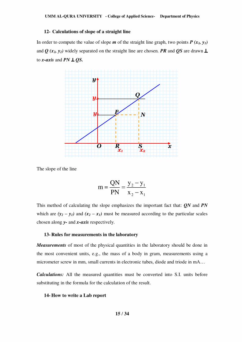
12- Calculations of slope of a straight line
In order to compute the value of slope m of the straight line graph, two points P (x1, y1)
and Q (x2, y2) widely separated on the straight line are chosen. PR and QS are drawn
to x-axis and PN QS.
The slope of the line
12
12
xxyy
PNQN= m
This method of calculating the slope emphasizes the important fact that: QN and PN
which are (y2 – y1) and (x2 – x1) must be measured according to the particular scales
chosen along y- and x-axis respectively.
13- Rules for measurements in the laboratory
Measurements of most of the physical quantities in the laboratory should be done in
the most convenient units, e.g., the mass of a body in gram, measurements using a
micrometer screw in mm, small currents in electronic tubes, diode and triode in mA…
Calculations: All the measured quantities must be converted into S.I. units before
substituting in the formula for the calculation of the result.
14- How to write a Lab report
y
xO R
N
S
P
Q
y1
y2
x1 x2
UMM AL-QURA UNIVERSITY - College of Applied Science- Department of Physics
16 / 34
A neat and systematic recording of the experiment in the practical file is very
important in achieving the success of the experimental investigations. The students
may write the experiment under the following heads in their fair practical notebooks.
Date: ............. , Experiment Name: ..............
Experiment No.: ……………….. , Page No.: ..............
1. Object/Aim: The object of the experiment to be performed should be clearly and
precisely stated.
2. Apparatus used: The main apparatus needed for the experiment are to be given
under this head. If any special assembly of apparatus is needed for the experiment, its
description should also be given in brief and its diagram should be drawn.
Diagram: A circuit diagram for electricity experiments and a ray diagram for light
experiment is a must. Simply principle diagram wherever needed, should be drawn
neatly.
3. Theory: The principle underlying the experiment should be mentioned.
4. The Formula used: The formula used should also be written explaining clearly the
symbols involved. Derivation of the formula may not be required.
5. Procedure/Method: The various steps to be followed in setting the apparatus and
taking the measurements should be written in the right order as per the requirement of
the experiment.
6. Observation: The observations and their recording, is the heart of the experiment.
As far as possible, the observations should be recorded in the tabular form neatly and
without any over-writing. In case of wrong entry, the wrong reading should be scored
by drawing a horizontal line over it and the correct reading should be written by its
side. On the top of the observation table the least counts and ranges of various
measuring instruments used should be clearly given. If the result of the experiment
depends upon certain environmental conditions like temperature; pressure, place, etc.,
then the values of these factors should also be mentioned.
UMM AL-QURA UNIVERSITY - College of Applied Science- Department of Physics
17 / 34
7. Calculations: The observed values of various quantities should be substituted in the
formula and the computations should be done systematically and neatly. Wherever
possible, graphical method for obtaining results should be employed.
8. The Results: The conclusion drawn from the experimental observations has to be
stated under this heading. If the result is in the form of a numerical value of a physical
quantity, it should be expressed in its proper unit. Also mention the physical conditions
like temperature, pressure, etc., if the result happens to depend upon them.
9. Error: Percentage error may also be calculated if the standard value of the result is
known.
10. Sources of error and precaution: The possible errors which are beyond the control
of the experimenter and which affect the result should be mentioned here. The
precautions which are actually observed during the course of the experiment should be
mentioned under this heading.
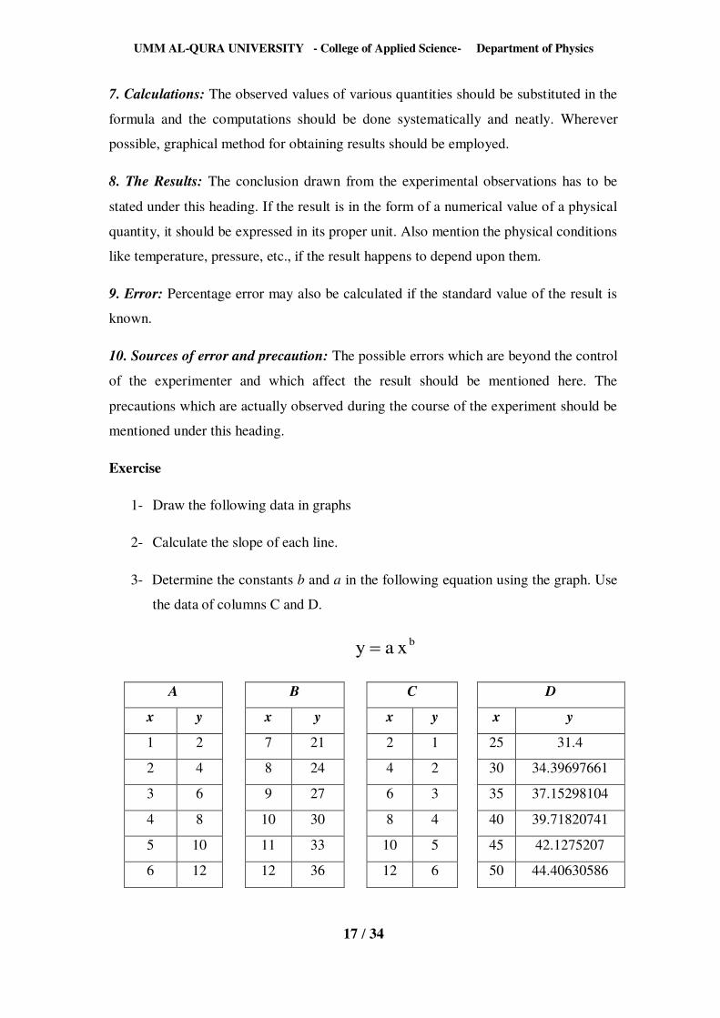
Exercise
1- Draw the following data in graphs
2- Calculate the slope of each line.
3- Determine the constants b and a in the following equation using the graph. Use
the data of columns C and D.
bxay
A B C D
x y x y x y x y
1 2 7 21 2 1 25 31.4
2 4 8 24 4 2 30 34.39697661
3 6 9 27 6 3 35 37.15298104
4 8 10 30 8 4 40 39.71820741
5 10 11 33 10 5 45 42.1275207
6 12 12 36 12 6 50 44.40630586
UMM AL-QURA UNIVERSITY - College of Applied Science- Department of Physics
18 / 34
Experiment: THE SIMPLE PENDULUM
Objective: The study of the physical properties of the basic simple pendulum
Apparatus: String, pendulum bob, meter stick and Stop watch
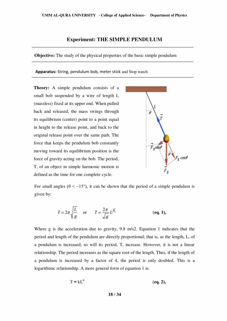
Theory: A simple pendulum consists of a
small bob suspended by a wire of length L
(massless) fixed at its upper end. When pulled
back and released, the mass swings through
its equilibrium (center) point to a point equal
in height to the release point, and back to the
original release point over the same path. The
force that keeps the pendulum bob constantly
moving toward its equilibrium position is the
force of gravity acting on the bob. The period,
T, of an object in simple harmonic motion is
defined as the time for one complete cycle.
For small angles (θ < ~15°), it can be shown that the period of a simple pendulum is
given by:
Where g is the acceleration due to gravity, 9.8 m/s2. Equation 1 indicates that the
period and length of the pendulum are directly proportional; that is, as the length, L, of
a pendulum is increased, so will its period, T, increase. However, it is not a linear
relationship. The period increases as the square root of the length. Thus, if the length of
a pendulum is increased by a factor of 4, the period is only doubled. This is a
logarithmic relationship. A more general form of equation 1 is:
UMM AL-QURA UNIVERSITY - College of Applied Science- Department of Physics
19 / 34
Whereg
2k and the exponent n is ½. Rearranging this expression for k yields:
Taking the log10 of both sides of equation 2 yields:
Comparing this to y = mx + b (the equation of a straight line), we can see that if the
period vs. the length of the pendulum were plotted on a graph with logarithmic axes,
then the slope of the line would equal n and the y-intercept would be equal to the value
of log10 k. Also from equation 2, it can be seen that for a pendulum whose length were
1 m (L = 1), then Ln = 1. Therefore,
Procedure:
1. part I : Dependence of Period on Mass
A mass is attached to the other end of the string and pulled back and let go, so that it
executes (approximately) simple harmonic motion. The time required to complete 50
cycles (t) is measured with a stopwatch and recorded. To improve accuracy, three trials
are completed for each measurement. The average of the recorded values of t for the
three trials is then divided by 50 to obtain the period (T) of the motion. In the first part
of the experiment, the length L of the string is kept constant at 30 cm and different masses are attached to its end to determine the dependence of the period on mass. All
times are measured in seconds. The mass is measured in grams, and then converted to
kilograms.
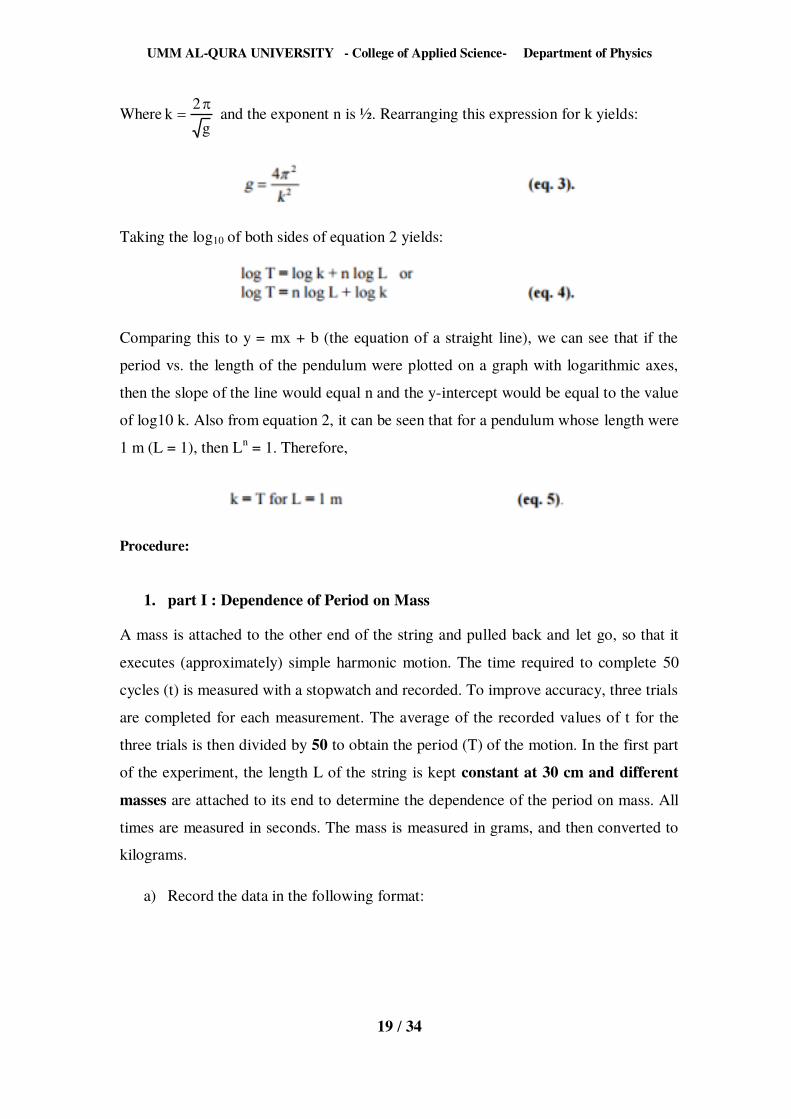
a) Record the data in the following format:
UMM AL-QURA UNIVERSITY - College of Applied Science- Department of Physics
20 / 34
m(g) m(Kg) t1(s) t2(s) t3(s) tavg (s) T= tavg/50
Table 1: Period T vs. Mass m for Simple Pendulum. ( L= 30 cm)
b) Plot T vs. m. (fig.1)
c) From the graph (question b), the period of a simple pendulum is dependent of
mass?
2. part II : Dependence of Period on Length
The mass (m) is held constant at 100 g and the length (L) is varied from 30 cm to 100 cm, in 10 cm increments. Times are measured and period calculated as in part I.
As before, all times are in seconds. Lengths are measured in centimeters, then
converted to m.
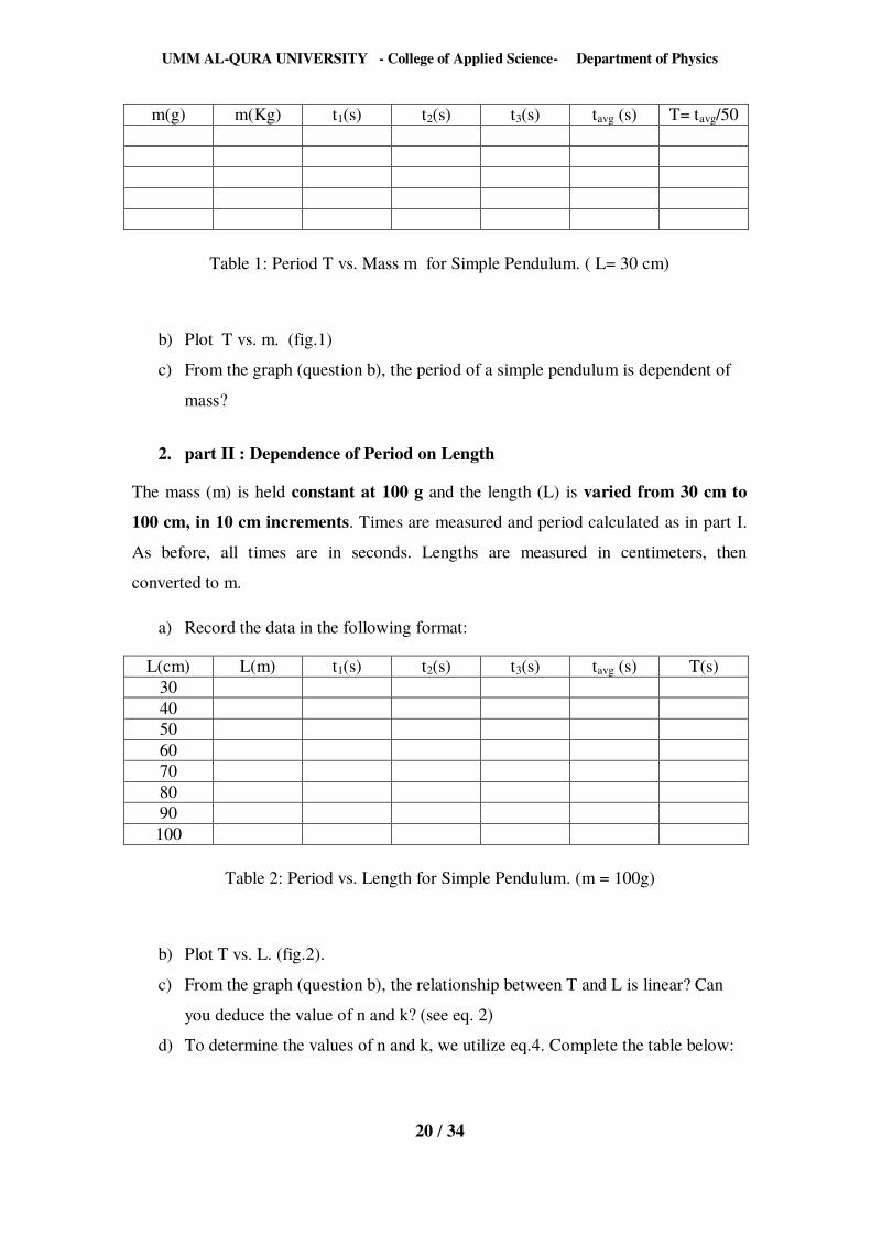
a) Record the data in the following format:
L(cm) L(m) t1(s) t2(s) t3(s) tavg (s) T(s) 30 40 50 60 70 80 90 100
Table 2: Period vs. Length for Simple Pendulum. (m = 100g)
b) Plot T vs. L. (fig.2).
c) From the graph (question b), the relationship between T and L is linear? Can
you deduce the value of n and k? (see eq. 2)
d) To determine the values of n and k, we utilize eq.4. Complete the table below:
UMM AL-QURA UNIVERSITY - College of Applied Science- Department of Physics
21 / 34
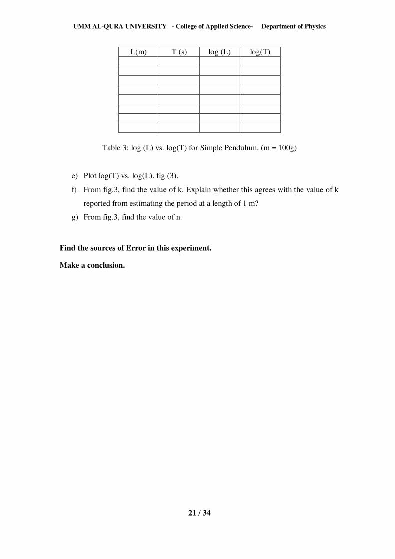
L(m) T (s) log (L) log(T)
Table 3: log (L) vs. log(T) for Simple Pendulum. (m = 100g)
e) Plot log(T) vs. log(L). fig (3).
f) From fig.3, find the value of k. Explain whether this agrees with the value of k
reported from estimating the period at a length of 1 m?
g) From fig.3, find the value of n.
Find the sources of Error in this experiment.
Make a conclusion.
UMM AL-QURA UNIVERSITY - College of Applied Science- Department of Physics
22 / 34
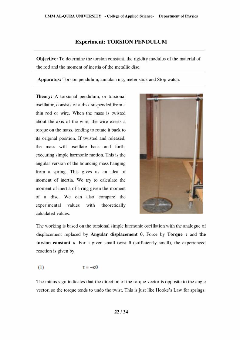
Experiment: TORSION PENDULUM
Objective: To determine the torsion constant, the rigidity modulus of the material of
the rod and the moment of inertia of the metallic disc.
Apparatus: Torsion pendulum, annular ring, meter stick and Stop watch.
Theory: A torsional pendulum, or torsional
oscillator, consists of a disk suspended from a
thin rod or wire. When the mass is twisted
about the axis of the wire, the wire exerts a
torque on the mass, tending to rotate it back to
its original position. If twisted and released,
the mass will oscillate back and forth,
executing simple harmonic motion. This is the
angular version of the bouncing mass hanging
from a spring. This gives us an idea of
moment of inertia. We try to calculate the
moment of inertia of a ring given the moment
of a disc. We can also compare the
experimental values with theoretically
calculated values.
The working is based on the torsional simple harmonic oscillation with the analogue of
displacement replaced by Angular displacement θ, Force by Torque τ and the torsion constant κ. For a given small twist θ (sufficiently small), the experienced
reaction is given by
The minus sign indicates that the direction of the torque vector is opposite to the angle
vector, so the torque tends to undo the twist. This is just like Hooke’s Law for springs.
UMM AL-QURA UNIVERSITY - College of Applied Science- Department of Physics
23 / 34
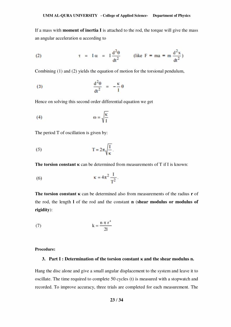
If a mass with moment of inertia I is attached to the rod, the torque will give the mass
an angular acceleration α according to
Combining (1) and (2) yields the equation of motion for the torsional pendulum,
Hence on solving this second order differential equation we get
The period T of oscillation is given by:
The torsion constant κ can be determined from measurements of T if I is known:
The torsion constant κ can be determined also from measurements of the radius r of
the rod, the length l of the rod and the constant n (shear modulus or modulus of rigidity):
l2rnk)7(
4
Procedure:
3. Part I : Determination of the torsion constant κ and the shear modulus n.
Hang the disc alone and give a small angular displacement to the system and leave it to
oscillate. The time required to complete 50 cycles (t) is measured with a stopwatch and
recorded. To improve accuracy, three trials are completed for each measurement. The
UMM AL-QURA UNIVERSITY - College of Applied Science- Department of Physics
24 / 34
average of the recorded values of t for the three trials is then divided by 50 to obtain
the period (T) of the motion.
d) Record the data in the following format:
t1(s) t2(s) t3(s) tavg (s) T= tavg/50
Table 1: Period of oscillation for Torsion Pendulum (disk only).
e) Measure the theoretical values of the moment of inertia of the disk. Record
below.
Mdisk = …………………….Kg
Rdisk = …………………….m
2diskdiskdisk RM
21.)theo(I = ………………………….
f) Calculate the torsion constant κ (From eq. 6)
The torsion constant κ = …………………………….
g) Calculate the modulus of rigidity n :
rrod = …………………….m
lrod = …………………….m
The modulus of rigidity n (From eq.7) = …………………………….
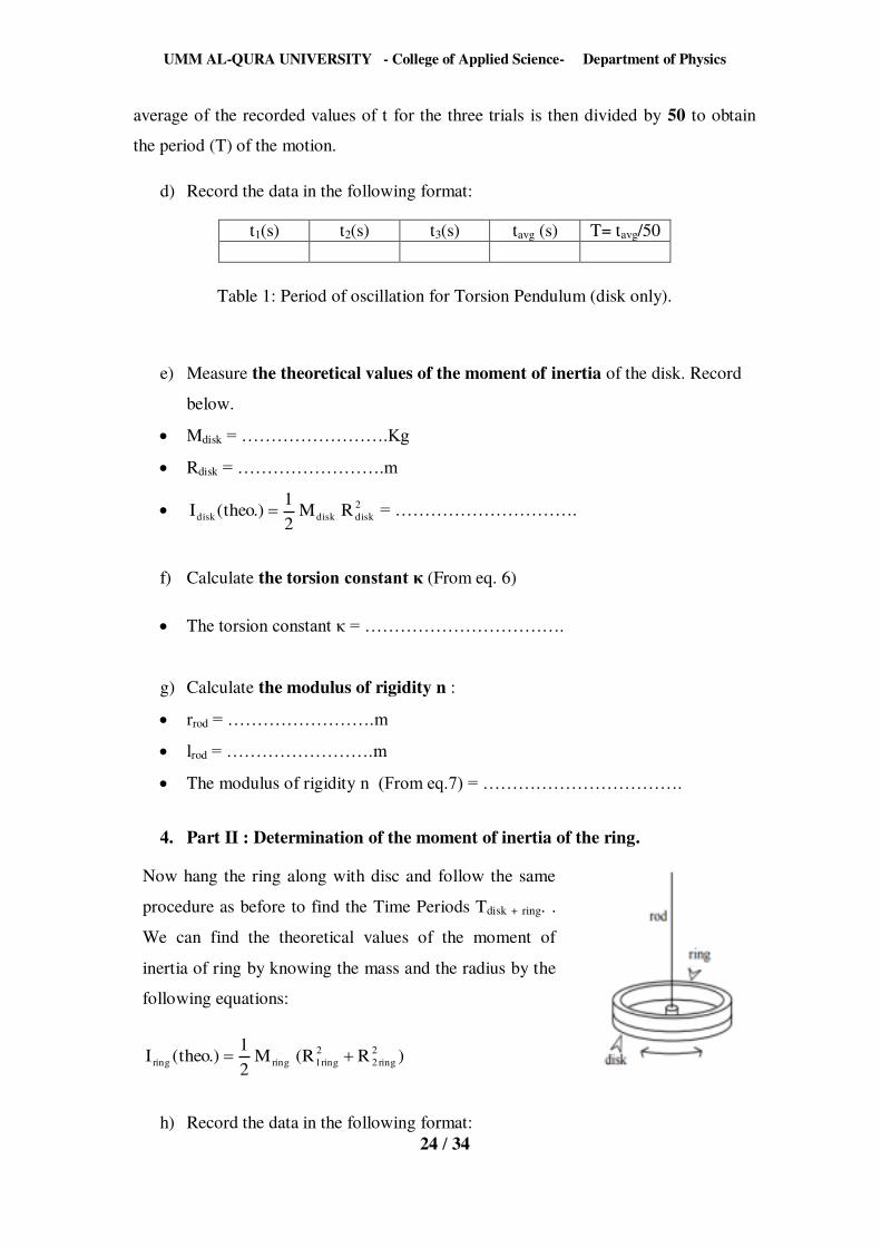
4. Part II : Determination of the moment of inertia of the ring.
Now hang the ring along with disc and follow the same
procedure as before to find the Time Periods Tdisk + ring. .
We can find the theoretical values of the moment of
inertia of ring by knowing the mass and the radius by the
following equations:
)RR(M21.)theo(I 2
ring22ring1ringring
h) Record the data in the following format:
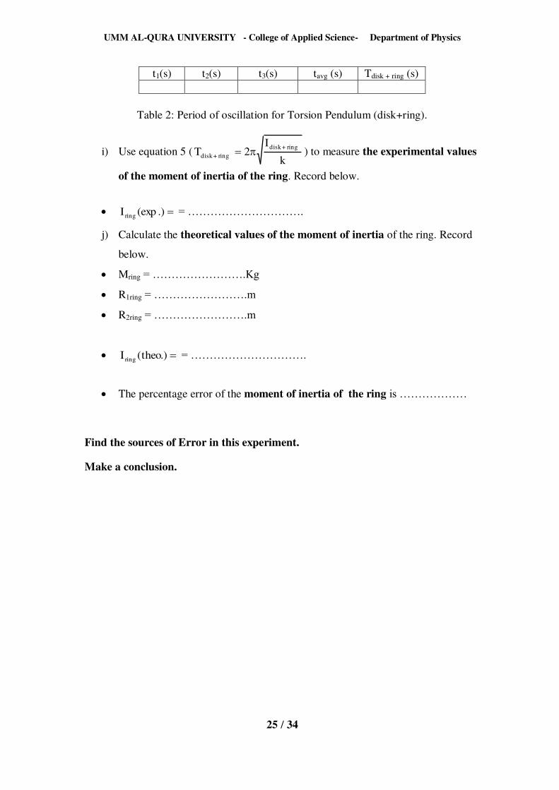
UMM AL-QURA UNIVERSITY - College of Applied Science- Department of Physics
25 / 34
t1(s) t2(s) t3(s) tavg (s) Tdisk + ring (s)
Table 2: Period of oscillation for Torsion Pendulum (disk+ring).
i) Use equation 5 (k
I2T ring +disk
ring +disk ) to measure the experimental values
of the moment of inertia of the ring. Record below.
.)(expIring = ………………………….
j) Calculate the theoretical values of the moment of inertia of the ring. Record
below.
Mring = …………………….Kg
R1ring = …………………….m
R2ring = …………………….m
.)theo(Iring = ………………………….
The percentage error of the moment of inertia of the ring is ………………
Find the sources of Error in this experiment.
Make a conclusion.
UMM AL-QURA UNIVERSITY - College of Applied Science- Department of Physics
26 / 34
Experiment: MOMENT OF INERTIA
Objective: To measure the moments of inertia of several objects
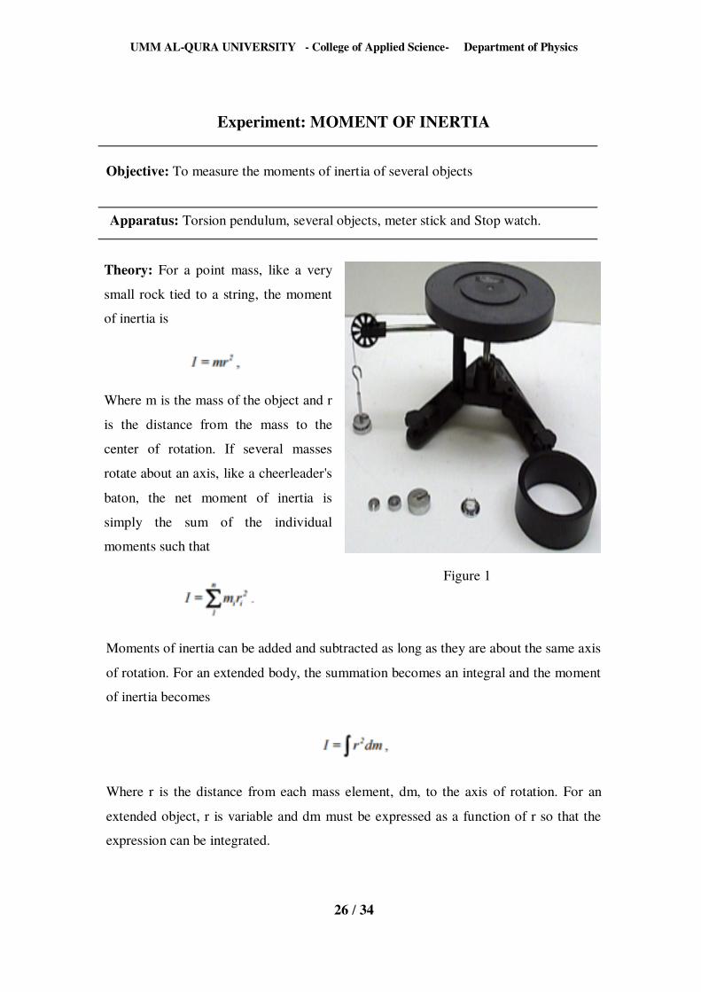
Apparatus: Torsion pendulum, several objects, meter stick and Stop watch.
Theory: For a point mass, like a very
small rock tied to a string, the moment
of inertia is
Where m is the mass of the object and r
is the distance from the mass to the
center of rotation. If several masses
rotate about an axis, like a cheerleader's
baton, the net moment of inertia is
simply the sum of the individual
moments such that
Figure 1
Moments of inertia can be added and subtracted as long as they are about the same axis
of rotation. For an extended body, the summation becomes an integral and the moment
of inertia becomes
Where r is the distance from each mass element, dm, to the axis of rotation. For an
extended object, r is variable and dm must be expressed as a function of r so that the
expression can be integrated.
UMM AL-QURA UNIVERSITY - College of Applied Science- Department of Physics
27 / 34
A torque will be applied to the base by putting weight on a string that winds around the
axe. Applying Newton’s Second Law to the masses allows us to show that the total
tension in the string is related to the acceleration of the masses by: T = mg – ma. The
moment of inertia of each system can be experimentally found using the formula:
)1ag(RmI 2
Procedure:
The setup for the experiment is depicted in Figure 1. A string is tied around one hub of
the pulley, and the other end is tied to a weight hanger, where we suspend (including
the hanger) masses of roughly 10 g, 25 g and 50 g. The mass is allowed to fall a
distance h.
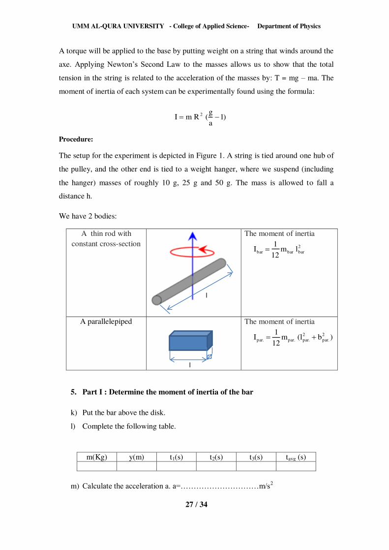
We have 2 bodies:
A thin rod with constant cross-section
The moment of inertia 2barbarbar lm
121I
A parallelepiped The moment of inertia
)bl(m121I 2
.par2
.par.par.par
5. Part I : Determine the moment of inertia of the bar
k) Put the bar above the disk.
l) Complete the following table.
m(Kg) y(m) t1(s) t2(s) t3(s) tavg (s)
m) Calculate the acceleration a. a=…………………………m/s2
l
l
UMM AL-QURA UNIVERSITY - College of Applied Science- Department of Physics
28 / 34
n) From equation: )1ag(RmI 2
diskbardisk , bardiskI =…………………Kg m2
o) 2disk
2diskbardiskbar mKg.................Rm
21II
p) Calculate the absolute and the percentage error.
q) Remove the bar from the rotating assembly. Replace it with the parallelepiped.
r) Repeat the previous steps to determine the moment of inertia of the parallelepiped.
Find the sources of Error in this experiment.
Make a conclusion
UMM AL-QURA UNIVERSITY - College of Applied Science- Department of Physics
29 / 34
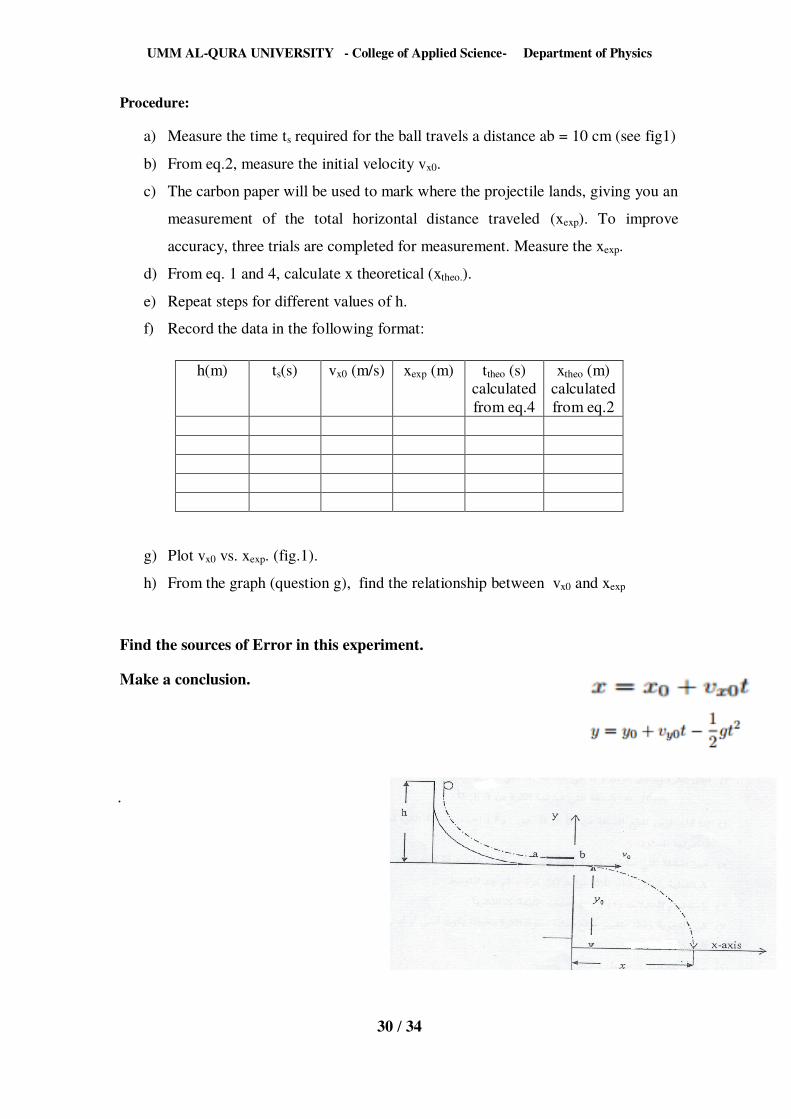
Experiment: PROJECTILES MOTION
Objective: Study two dimensional projectile motion of an object in free fall
Apparatus: Projectile launcher, plastic ball, carbon paper and meter stick
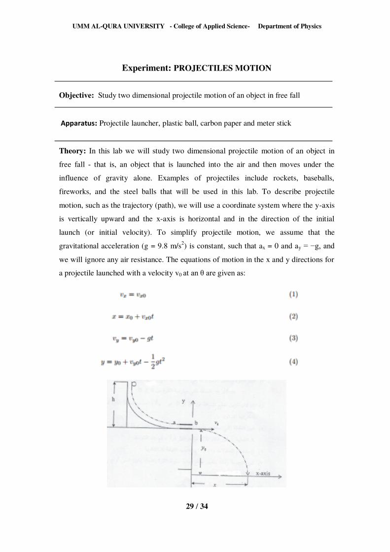
Theory: In this lab we will study two dimensional projectile motion of an object in
free fall - that is, an object that is launched into the air and then moves under the
influence of gravity alone. Examples of projectiles include rockets, baseballs,
fireworks, and the steel balls that will be used in this lab. To describe projectile
motion, such as the trajectory (path), we will use a coordinate system where the y-axis
is vertically upward and the x-axis is horizontal and in the direction of the initial
launch (or initial velocity). To simplify projectile motion, we assume that the
gravitational acceleration (g = 9.8 m/s2) is constant, such that ax = 0 and ay = −g, and
we will ignore any air resistance. The equations of motion in the x and y directions for
a projectile launched with a velocity v0 at an θ are given as:
UMM AL-QURA UNIVERSITY - College of Applied Science- Department of Physics
30 / 34
Procedure:
a) Measure the time ts required for the ball travels a distance ab = 10 cm (see fig1)
b) From eq.2, measure the initial velocity vx0.
c) The carbon paper will be used to mark where the projectile lands, giving you an
measurement of the total horizontal distance traveled (xexp). To improve
accuracy, three trials are completed for measurement. Measure the xexp.
d) From eq. 1 and 4, calculate x theoretical (xtheo.).
e) Repeat steps for different values of h.
f) Record the data in the following format:
h(m) ts(s) vx0 (m/s) xexp (m) ttheo (s) calculated from eq.4
xtheo (m) calculated from eq.2
g) Plot vx0 vs. xexp. (fig.1).
h) From the graph (question g), find the relationship between vx0 and xexp
Find the sources of Error in this experiment.
Make a conclusion.
UMM AL-QURA UNIVERSITY - College of Applied Science- Department of Physics
31 / 34
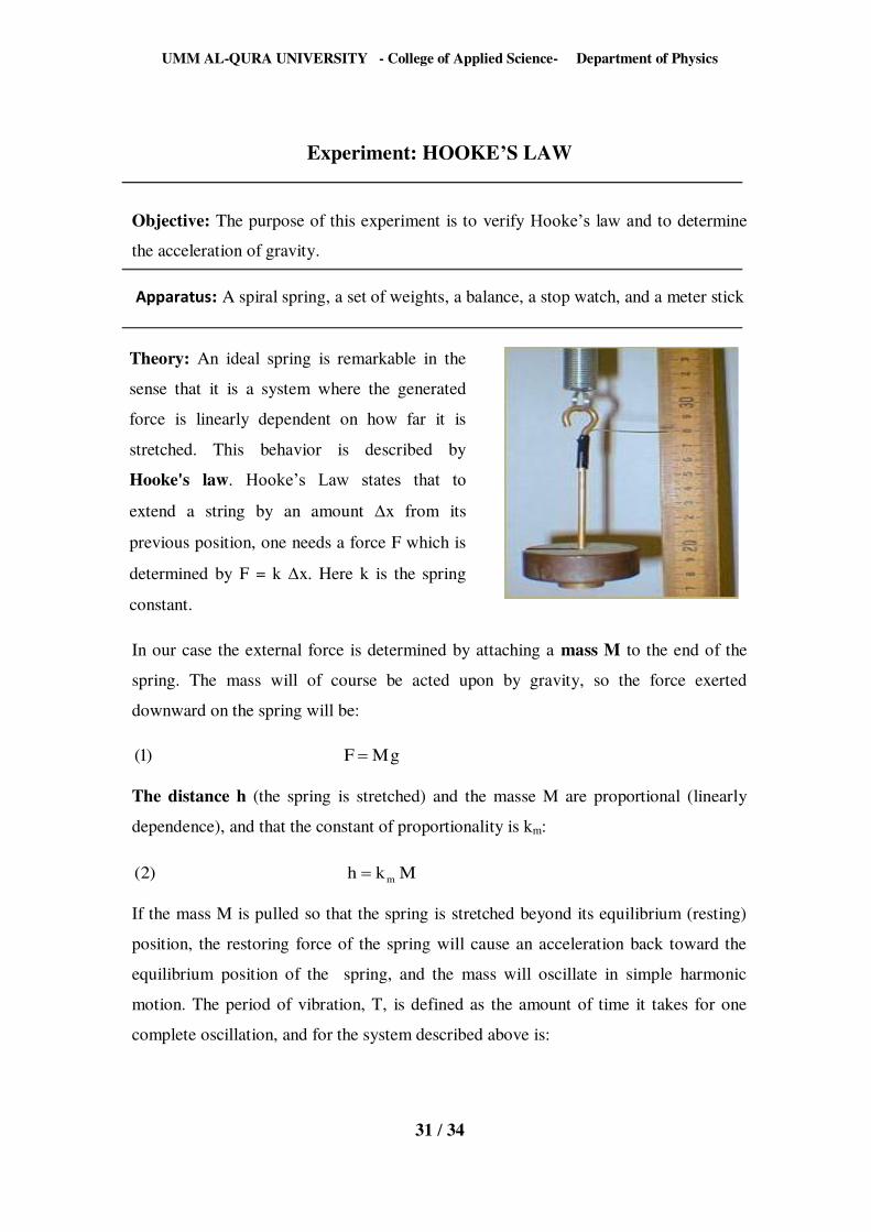
Experiment: HOOKE’S LAW
Objective: The purpose of this experiment is to verify Hooke’s law and to determine
the acceleration of gravity.
Apparatus: A spiral spring, a set of weights, a balance, a stop watch, and a meter stick
Theory: An ideal spring is remarkable in the
sense that it is a system where the generated
force is linearly dependent on how far it is
stretched. This behavior is described by
Hooke's law. Hooke’s Law states that to
extend a string by an amount x from its
previous position, one needs a force F which is
determined by F = k x. Here k is the spring
constant.
In our case the external force is determined by attaching a mass M to the end of the
spring. The mass will of course be acted upon by gravity, so the force exerted
downward on the spring will be:
gMF)1(
The distance h (the spring is stretched) and the masse M are proportional (linearly
dependence), and that the constant of proportionality is km:
Mkh)2( m
If the mass M is pulled so that the spring is stretched beyond its equilibrium (resting)
position, the restoring force of the spring will cause an acceleration back toward the
equilibrium position of the spring, and the mass will oscillate in simple harmonic
motion. The period of vibration, T, is defined as the amount of time it takes for one
complete oscillation, and for the system described above is:
UMM AL-QURA UNIVERSITY - College of Applied Science- Department of Physics
32 / 34
g)mM(k2T)3( m
Where (M+m) is the equivalent mass of the system, that is, the sum of the mass, M,
which hangs from the spring and the spring's equivalent mass, m.
Squaring both sides of the equation 3 yields:
g)mM(k4T)4( m22
Expanding the equation 4:
mg
k4Mg
k4T)5( m2m22
Therefore, if we perform an experiment in which the mass hanging at the end of the
spring (the independent variable) is varied and measure the period squared (T2 ; the
dependent variable), we can plot the data and fit it linearly. Comparing equation 5 to
the equation for a straight line (y = ax + b), we see that the slope and y-intercept,
respectively, of the linear fit is:
Slope = g
k4 m2 and y- intercept = mg
k4 m2
Procedure:
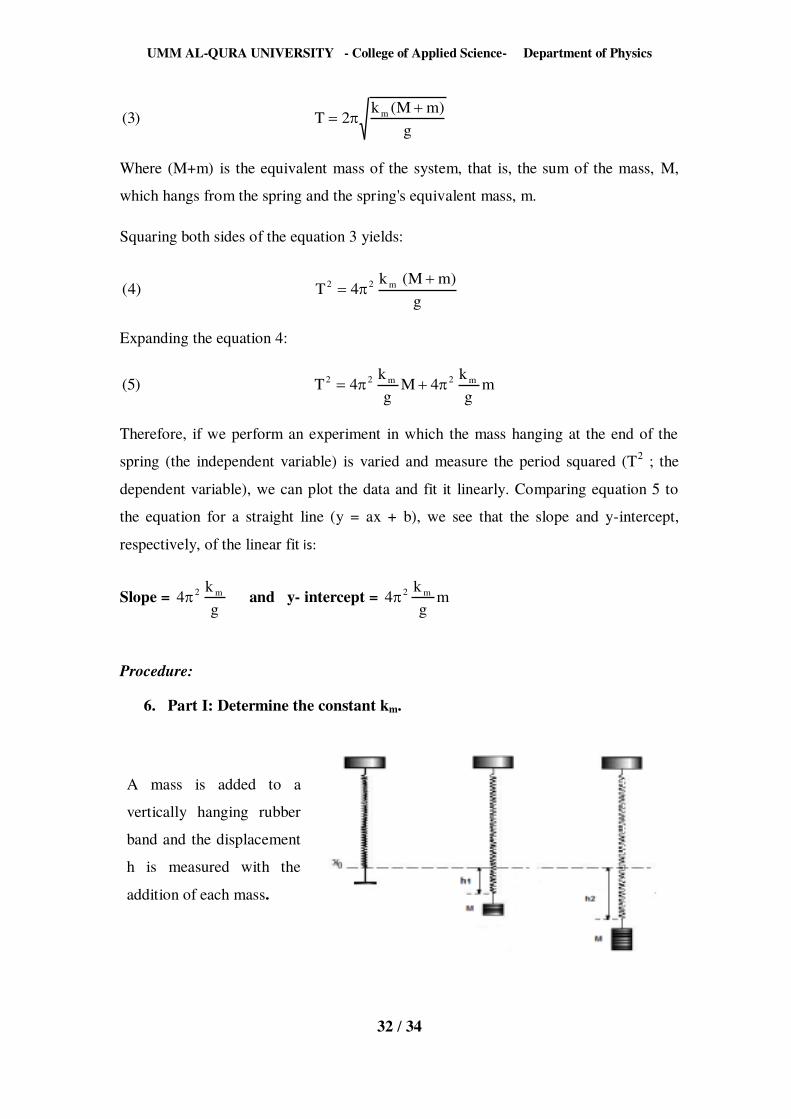
6. Part I: Determine the constant km.
A mass is added to a
vertically hanging rubber
band and the displacement
h is measured with the
addition of each mass.
UMM AL-QURA UNIVERSITY - College of Applied Science- Department of Physics
33 / 34
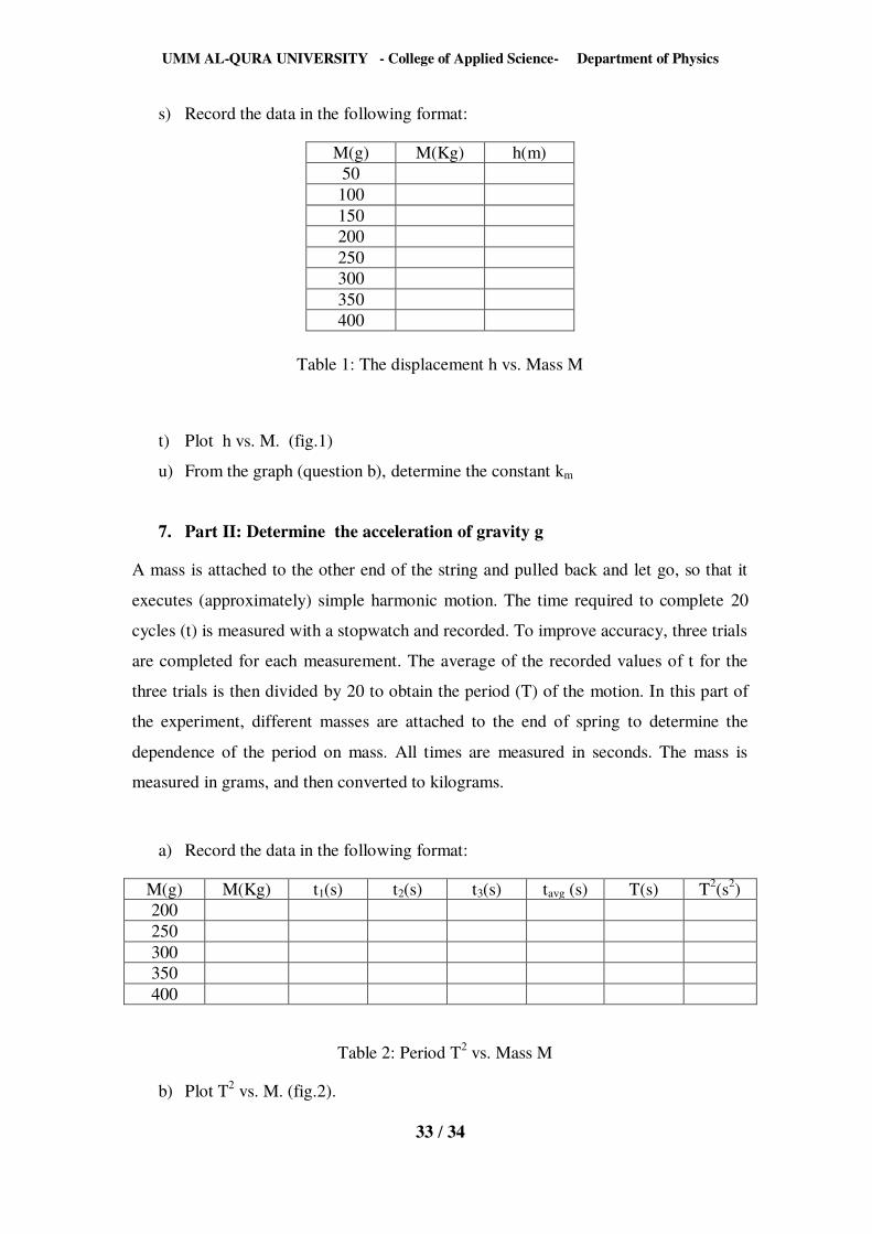
s) Record the data in the following format:
M(g) M(Kg) h(m) 50 100 150 200 250 300 350 400
Table 1: The displacement h vs. Mass M
t) Plot h vs. M. (fig.1)
u) From the graph (question b), determine the constant km
7. Part II: Determine the acceleration of gravity g
A mass is attached to the other end of the string and pulled back and let go, so that it
executes (approximately) simple harmonic motion. The time required to complete 20
cycles (t) is measured with a stopwatch and recorded. To improve accuracy, three trials
are completed for each measurement. The average of the recorded values of t for the
three trials is then divided by 20 to obtain the period (T) of the motion. In this part of
the experiment, different masses are attached to the end of spring to determine the
dependence of the period on mass. All times are measured in seconds. The mass is
measured in grams, and then converted to kilograms.
a) Record the data in the following format:
M(g) M(Kg) t1(s) t2(s) t3(s) tavg (s) T(s) T2(s2) 200 250 300 350 400
Table 2: Period T2 vs. Mass M
b) Plot T2 vs. M. (fig.2).

UMM AL-QURA UNIVERSITY - College of Applied Science- Department of Physics
34 / 34
c) From the graph (question b), the relationship between T2 and M is linear.
Deduce from the slop the value of the acceleration of gravity g and from the
y- intercept the value of the mass m. km is determined in part I.
d) Given that greal= 9.8 m.s2, calculate the absolute and the percentage error.
Find the sources of Error in this experiment.
Make a conclusion.
Related Documents