Physics 566: Quantum Optics Quantization of the ...

Page 1

Physics 566: Quantum OpticsQuantization of the Electromagnetic Field

Maxwell's Equations and Gauge invariance

In lecture we learned how to quantize a one dimensional scalar field corresponding tovibrations on an elastic rod. The procedure involved decomposing the field into its normalmodes of oscillation and then quantizing each mode as a simple harmonic oscillator. Wenow want to apply this procedure to the electromagnetic field. One might think of this aquantization of the vibrational modes of the "ether" in the pre-relativity description ofelectrodynamics. The dynamics of this field are determined by Maxwell's equations, which in the absenceof charges (and in CGS units) read

— ⋅ E = 0 , — ¥ E = -1c

∂B∂t

, — ⋅ B = 0 , — ¥ B =1c

∂E∂t

.

In contrast to our discussion of the quantization of the scalar field, this problem iscomplicated by two factors. First we are dealing with a three dimensional field, and secondit is a vector field. A vector field in three dimensions should be describable in terms of threescalar fields. However, at this point we have described our field in terms of six fields{Ex , Ey , Ez , Bx ,By , Bz}. We can get a description of the dynamics with fewer fields by

using the vector a scalar potentials, which transforms like the four vector in Minkowskispace, Am = (f, A) . The physical fields which exert forces on the charges are the electric anmagnetic fields which are defined in terms of the four-potential as

E = -—f -1c

∂A∂t

, B = — ¥ A .

The equation of motion for f and A follow from Maxwell's equations

—2f = -1c

∂

∂t— ⋅ A

—2A -1c

∂2

∂t2 A = -— — ⋅ A +1c

∂f∂t

Ê Ë

ˆ ¯

At this point the four components of Am describe our field. This set is actually overcomplete. One of the fundamental properties of Maxwell's equation is gauge invariance.

Page 2

That is, the physical fields E and B are unchanged if we redefine our four potential bymaking the transformation Am Æ Am + ∂m c , or in terms of the components

f Æ f +1c

∂c∂t

, A Æ A + —c

where c is an arbitrary scalar field.

Maxwell's Equations in the Coloumb Gauge

The choice of gauge is completely arbitrary. For quantization of the field the convenientchoice is the Coulomb gauge (a name we will understand soon) which is defined bychoosing the vector potential such that

— ⋅ A = 0 .

This is known as the "transversality" condition. If the vector potential we start with does notsatisfy this condition it is always possible to make a gauge transformation so that A istransverse by choosing a gauge function that satisfies —2c = 0 . The equation for the scalarpotential is the Laplace's equation,

—2f = 0 .

Thus, f is no longer a dynamical variable. It is just depends on the geometry of theproblem, and is constant in time. The equation of motion for A^ (where ^ indicates that Asatisfies the transversality condition) is the wave equation,

—2A^ -1c

∂2

∂t2 A^ = 0 .

The only remaining dynamical field which we must quantize is A^. The dynamical

physical fields are E^ = -1c

∂A ^

∂t and B^ = — ¥ A^ .

The name Coulomb gauge becomes clear when we include the sources: charge density r,and current density J. In the Coulomb gauge, the equations are

Page 3

—2f = 4pr

—2A^ -1c

∂2

∂t2 A^ = -4pc

J^

The first equation is Poisson's equation, now defined for the instantaneous charge density(which may be time varying), whose solution is

f (x, t) = d3 ¢ x r( ¢ x ,t)x - ¢ x Ú .

This is just the instantaneous Coulomb potential, and hence the name of the gauge. Notethere is no retarded time in this integral. That is, the potential at time t and a point x isinstantaneously related to the charge density at a distant point x' the same time. One mightworry if the causal laws of special relativity are violated by this fact. Of course this is notthe case for the original Maxwell equation were Lorentz invariant, and thus satisfy all thecausal laws we know and love. Remember that the physical fields are E and B. Thesealways satisfy causal equations of motion, no matter what gauge we choose. The Coulombgauge is a bit bizarre in that f seems to be related to the instantaneous values of the source.However, this effect is canceled by the fact that the vector potential is not driven by thephysical current, but only by the "transverse" part of J, which itself has an instantaneouspart. In fact the transversality condition is itself dependent on the choice of reference frame(i.e. it is not manifestly covariant). However, we again emphasize that no laws of relativityare violated.

Normal Modes in the Coulomb Gauge

In order to quantize the field by the procedure we developed in lecture notes on"quantum field theory", we must introduce a normal mode expansion for the field. Ourdynamical variable is the transverse delta function A^, which satisfies the wave equation.To arrive at a discrete set of modes, we will introduce an artificial "quantization volume" inthe same way that we took a finite length of rod in our study of the vibrational modes for ascalar field. We will take periodic boundary conditions for complete generality to allow forpropagating solutions. The normal modes are then plane waves with a given polarization

uk ,l (x) =

r e k ,l

eik⋅x

V,

Page 4

where k =nx2p

Lex +

ny 2p

Ley +

nz 2pL

ez , for periodic boundary conditions in a volume

V=L3, for some integers {nx , ny ,nz}. The vectors

r e k ,l are the unit polarization vectors

perpendicular to wave vector k, k ⋅

r e k,l = 0 . This insures the transversality condition. The

parameter l (not to be confused with the wave length) is an index with value 1 or 2representing any two basis vectors in the plane perpendicular to k:

k

The polarization vectors,

r e k ,l , may be complex if they represent a general elliptic

polarization (for example right and left circularly polarized fields). The normal modes are orthogonal

d3x uk,l* (x) ⋅ u ¢ k , ¢ l (x)

VÚ = dk , ¢ k dl , ¢ l .

The completeness relation is a bit more complicated than for our scalar field. Consider thesum over all modes of the tensor uk,l

( i)*( ¢ x ) ⋅ uk,l

( j) (x) ,

uk,l(i)*

( ¢ x ) ⋅uk,l( j) (x)

k ,l =

eik ⋅( ¢ x -x)

Vk ek,l

(i )*

l e k,l

( j) .

The polarization vectors

r e k ,l span the plane perpendicular to k. Therefore

ek ,l(i)*

l ek,l

( j ) = di j - ˆ k i ˆ k j .

That is, d i j - ˆ k i ˆ k j is the tensor that projects any vector into the plane perpendicular to k.

The completeness relation reads,

Page 5

uk,l(i)*

( ¢ x ) ⋅uk,l( j) (x)

k ,l =

1V

di j - ˆ k i ˆ k j( )k eik⋅( ¢ x -x) = d^

i j(x - ¢ x ) .

The tensor, d^i j(x - ¢ x ) , is known as the "transverse" delta function, defined by the property

that it projects any vector field V(x) into the transverse component V^(x),

d3 ¢ x V i ( ¢ x )Ú d^i j(x - ¢ x ) = V^

j (x) , with zero divergence, — ⋅ V^ = 0 . Since the vector potential in the Coulomb gauge is transverse, it can be expanded in thecomplete set of normal mode functions uk ,l ,

A^ (x, t) =

2phc2

wka k,l (t)uk ,l (x) + ak,l

* (t) uk,l* (x)( )

k,l .

Here we have used the normal mode expansion for periodic boundary conditions, given onpage 12 of lecture "Intro. to Quantum Field Theory" in terms of the dimensionless complexamplitudes

ak ,l (t) = ak ,l (0)e-iw kt , where wk = c|k|.

The normalization constant,

2phc2

wk, is the appropriate scale factor q0,k. Substituting in

for the normal modes we obtain,

A^ (x, t) =

2phc2

w kVa k,l (0)

r e k,lei(k⋅x-w k t) + a k,l

* (0)r e k,l

* e-i( k⋅x -wkt )( )k,l .

The transverse component of the electric and magnetic fields can be written using thedefinition at the bottom of page 2

E^(x, t) = i 2phwk

Va k,l (0)

r e k,l ei( k⋅x -wk t) - a k,l

* (0)r e k,l

* e-i(k ⋅x- wkt)( )k,lÂ

B^ (x, t) = i 2phc2

Vwkak ,l (0)k ¥

r e k,l ei( k⋅x -wkt ) - a k,l

* (0)k ¥r e k,l

* e-i( k⋅x- wkt )( )k ,lÂ

Page 6

The Quantized Electromagnetic Field

Now that we've expanded the field in terms of its normal modes, we can immediatelyquantize it according the procedure in lecture. Thus, we associate the complex amplitudeswith creation and annihilation operators

ak ,l* (0) Æ ˆ a k,l

† , ak ,l (0) Æ ˆ a k,l ,

are instate canonical commutation relations

[ ˆ a k,l , ˆ a ¢ k , ¢ l † ] = dk, ¢ k dl , ¢ l .

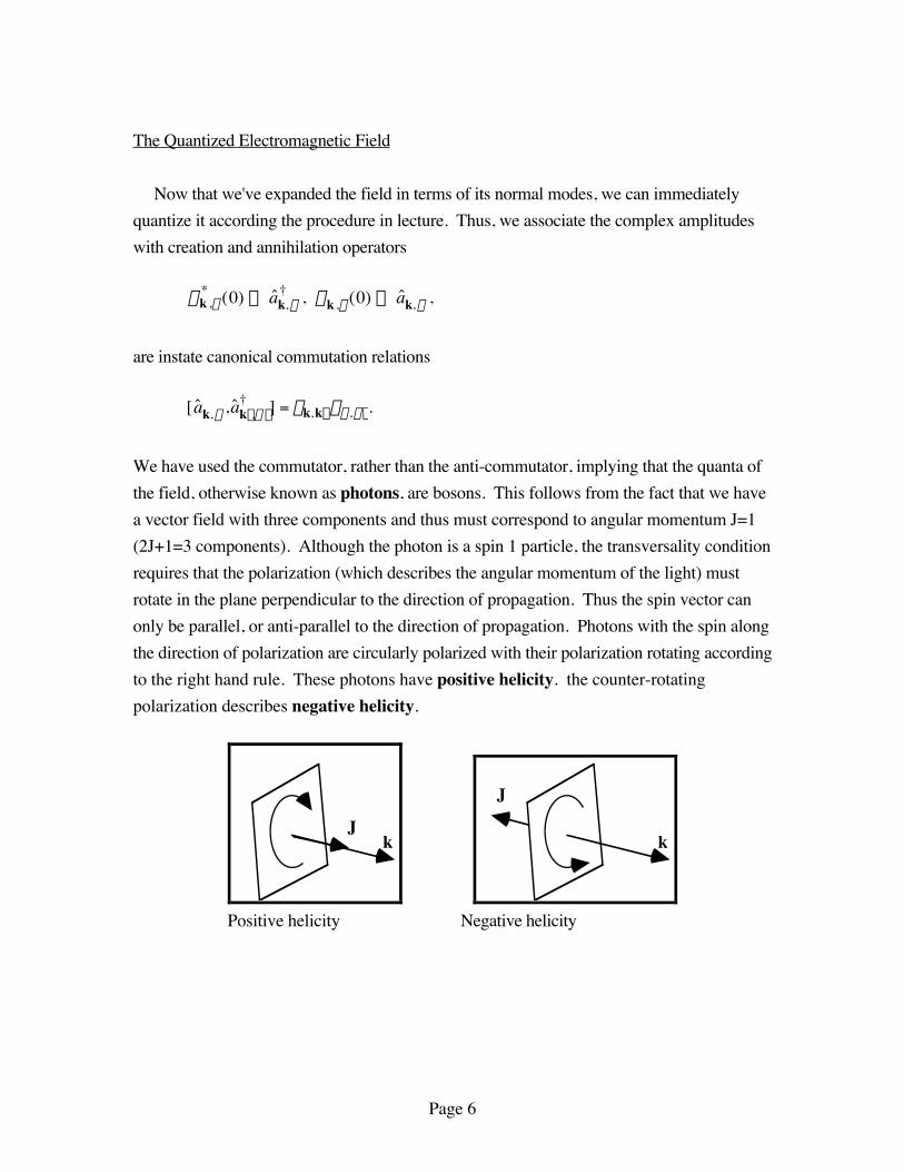
We have used the commutator, rather than the anti-commutator, implying that the quanta ofthe field, otherwise known as photons, are bosons. This follows from the fact that we havea vector field with three components and thus must correspond to angular momentum J=1(2J+1=3 components). Although the photon is a spin 1 particle, the transversality conditionrequires that the polarization (which describes the angular momentum of the light) mustrotate in the plane perpendicular to the direction of propagation. Thus the spin vector canonly be parallel, or anti-parallel to the direction of propagation. Photons with the spin alongthe direction of polarization are circularly polarized with their polarization rotating accordingto the right hand rule. These photons have positive helicity. the counter-rotatingpolarization describes negative helicity.

kJ

k

J

Positive helicity Negative helicity

Page 7

The classical fields now become vector operators,

ˆ A ̂ (x, t) =2phc2

Vwkˆ a k,l (0)

r e k,l ei( k⋅x -wkt ) + ˆ a k,l

† (0)r e k,l

* e- i(k⋅x-w kt)( )k,l ,

ˆ E ̂ (x, t) = i 2phwkV

ˆ a k ,l (0)r e k,lei(k ⋅x- wkt ) - ˆ a k,l

† (0)r e k,l

* e-i( k⋅x -wk t)( )k,l ,

) B ̂ (x, t) = i 2phc2

Vwkˆ a k,l (0)k ¥

r e k,lei(k ⋅x- wkt ) - ˆ a k,l

† (0)k ¥r e k,l

* e- i(k⋅x-w k t)( )k ,l .

The Hilbert space describing the quantized field is a Fock space. A state with n photons inthe mode with wave vector k and polarization l is given by acting with the creation operatorˆ a k,l

†n times on the vacuum state, and normalizing.

nk,l =( ˆ a k,l

† )n

n!0 .

Any state will be a superposition of such states for all modes. At times one will see the field operator decomposed as

ˆ E ̂ (x, t) = ˆ E ̂(+ )(x, t) + ˆ E ̂(-) (x, t)

where

ˆ E ̂(+ )(x, t) = i 2phw kV

ˆ a k,l (0)r e k,lei(k⋅x-w kt)

k ,l is known as the positive

frequency component of the electric field, and ˆ E ̂(- )(x, t) = ˆ E ̂(+) (x, t)( )† is known as the

negative frequency component. The positive frequency component contains onlyannihilation operators, and is thus responsible for absorption, while the negative frequencycomponents are responsible for emission of photons. From this picture, the "rotating wave"approximation, introduced in lecture for classical fields becomes clear. The dipoleinteraction Hamiltonian then has then form

ˆ H int = - ˆ d ⋅ ˆ E ̂(+ )(x, t) + ˆ E ̂(-) (x, t)( ) = - e ˆ d g e g + g e( ) ⋅ ˆ E ̂(+) (x, t) + ˆ E ̂(- )(x, t)( ) ª - e ˆ d g e g ˆ E ̂(+) (x, t) + g e ˆ E ̂(- )(x, t )( ) .

Page 8

That is, the annihilation of the photon is always accompanied by the transition of the atomfrom the ground to excited state, and the creation of a photon is accompanied by thetransition from the excited to ground state. The Hamiltonian of the field is given by the integral of the energy density over thequantization volume

ˆ H = 18p

d3x ˆ E ̂2

+ ˆ B ̂2Ê

Ë ˆ ¯ V

Ú .

If we write the field operators in terms of their normal mode expansions,

ˆ E ̂ (x, t) = i 2phw l ˆ a le- iw l tul (x) - ˆ a l†eiw lt ul

*(x)( )l ,

ˆ B ̂ (x, t) = i 2phc2

w lˆ a le

-iw ltkl ¥ ul (x) - ˆ a l†eiw l tkl ¥ ul

* (x)( )l ,

where l is a composite index for the mode (k,l), and ul (x) is the normal mode vectorfunction, then,

d3x ˆ E ̂VÚ

2= 2ph w lwm (- ˆ a l ˆ a me-i( w lt +wmt)

l,m d3xul (x)Ú ⋅ um (x)

+ ˆ a l† ˆ a me- i(w lt -wmt ) d3x ul

*(x)Ú ⋅ um (x) + H.c)

where H.c. stands for the Hermitian conjugate of the terms in parentheses. Using thecompleteness relations on the normal mode functions we have

d3x ul*(x)Ú ⋅ um(x) = dlm, d3xul (x)Ú ⋅ um(x) = d-lm

so that,

d3x ˆ E ̂

VÚ

2= 2phw l ( ˆ a l

† ˆ a l + ˆ a l ˆ a l† - ˆ a l ˆ a -le

-2iw l t

l - ˆ a l

† ˆ a - l† e2iw lt ) .

Similarly for the magnetic field we have,

Page 9

d3x ˆ B ̂VÚ

2=

2phc2

w lwm(- ˆ a l ˆ a me-i(w lt+ wmt)

l,m d3x(kl ¥ ulÚ ) ⋅ (km ¥ um )

+ ˆ a l† ˆ a me- i(w lt -wmt ) d3x(kl ¥ ul

* )Ú ⋅ (km ¥ u m) + H.c)

Using vector identities, and the fact that k ⋅ul = 0

(kl ¥ ul ) ⋅ (km ¥ um ) = (kl ⋅ km )(ul ⋅ um ) .

Therefore, the orthogonality relation yields,

d3x (kl ¥ ulÚ ) ⋅ (km ¥ u m) = -kl2 d- l,m ,

d3x (kl ¥ ul* )Ú ⋅ (km ¥ um ) = kl

2 d l,m .

The integral of the norm of the magnetic field operator is thus,

d3x ˆ B ̂

VÚ

2= 2phw l ( ˆ a l

† ˆ a l + ˆ a l ˆ a l† + ˆ a l ˆ a - le

-2iw lt

l + ˆ a l

† ˆ a - l† e2iw lt )

Finally we arrive at the expression for the Hamiltonian in terms of the creation andannihilation operators,

ˆ H = 12

hw k( ˆ a k,l†

ˆ a k ,l +k,l ˆ a k,l ˆ a k,l

†) = hwk ( ˆ a k,l

†ˆ a k,l +

k,lÂ

12

) ,

where we have reinstated the full indexing of the modes, and used the commutator to moveall the creation operators to the right. We recognize this Hamiltonian as the sum of simpleharmonic oscillator Hamiltonians for the modes.

Vacuum Fluctuations

In lecture we discussed that even in a state with no quanta, i.e. the vacuum 0 , thequantum uncertainties lead to fluctuations in the field. The average value of the electric fieldoperator vanishes in the vacuum,

Page 10

ˆ E

vac= 0

) E 0 = 0

) E (+ ) 0 + 0

) E (-) 0 = 0 ,

since

) E (+ ) 0 = i 2phwk

k,l uk,l (x)e-iw kt ˆ a k,l 0 = 0 , and

0

) E (-) =

) E (+) 0( )†

= 0.

However, the fluctuation of the field, given by the statistical variance, does not vanish

D ˆ E 2vac

= 0) E 2 0 - 0

) E 0 2

01 2 4 3 4

= 0) E (+ ) ⋅

) E (+ ) 0 + 0

) E (-) ⋅

) E (-) 0 + 0

) E (- ) ⋅

) E (+ ) 0 + 0

) E (+) ⋅

) E (-) 0

.

From the relation above 0) E (+ ) ⋅

) E (+) 0 = 0

) E (- ) ⋅

) E (- ) 0 = 0

) E (-) ⋅

) E (+) 0 = 0. Thus,

D ˆ E 2

vac= 0

) E (+ ) ⋅

) E (- ) 0 = 2ph w lwm

l,m ul

*(x) ⋅ um(x)e- i(w l -wm )t 0 ˆ a m ˆ a l† 0 ,

0 ˆ a m ˆ a l† 0 = 0 ˆ a l

† ˆ a m 00

1 2 4 3 4 + 0 [ ˆ a m, ˆ a l

†] 0d lm

1 2 4 4 3 4 4 = dlm

D ˆ E 2

vac= 0

) E (+ ) ⋅

) E (- ) 0 = 2phw k

k,l |uk,l (x)|2 =

2phwkVk,l

 .

Therefore, the vacuum fluctuation of the electric field is on the order of hwk / V per mode. The expectation value of the Hamiltonian in the vacuum is,

ˆ H vac

= 0 ˆ H 0 = hw k( 0 ˆ a k,l†

ˆ a k,l 0 +k,lÂ

12

) =hwk

2k ,l = • !

That is, each mode possesses a zero point energy

hwk2

, and for an infinite number of

modes in the vacuum the total vacuum energy goes to infinity! Such divergences plague themathematics of quantum field theory. A proper treatment requires the sophisticated theoryof renormalization. For our purposes we will use the physical argument that the true energyof the system must be measured with respect to the ground state energy, i.e. the energy ofthe vacuum. In other words, we will set the vacuum energy to zero. This is not to say the vacuum energy has no observable effects. In the next lecture wewill show that the vacuum fluctuations in the electromagnetic field are responsible for thedecay of an atom initially in the excited state to its ground sate. If we were able in someway to experimentally effect the environment of modes which interact with the atom, then we

Page 11

may be able to manipulate the vacuum fluctuations which interact with the atom and therebymodify the spontaneous emission rate with respect to the free space value. This may bedone by placing the atom in a highly reflecting cavity which alters the spectrum of modesthat can be supported inside. Such experiments have been performed. This a research fieldknown as "cavity QED", which again and again demonstrates the power of quantummechanics to describe the interactions of electromagnetic fields and atoms.