1 Lecture 4 Physics 1502: Lecture 25 Today’s Agenda • Announcements: • Midterm 2: NOT Nov. 6 – Following week … • Homework 07: due Friday next week • AC current – Resonances • Electromagnetic Waves – Maxwell’s Equations - Revised – Energy and Momentum in Waves L C ∼ ε R ω

Welcome message from author
This document is posted to help you gain knowledge. Please leave a comment to let me know what you think about it! Share it to your friends and learn new things together.
Transcript

1
Lecture 4
Physics 1502: Lecture 25Today’s Agenda
• Announcements:
• Midterm 2: NOT Nov. 6– Following week …
• Homework 07: due Friday next week• AC current
– Resonances
• Electromagnetic Waves– Maxwell’s Equations - Revised– Energy and Momentum in Waves
LC
∼ε
R
ω

2
Lecture 4
Phasors:LCR
⇒
⇓
Phasors:Tips• This phasor diagram was drawn as asnapshot of time t=0 with the voltagesbeing given as the projections along they-axis.
y
x
φimR
imXL
imXC
εm
“Full Phasor Diagram”
From this diagram, we can also create atriangle which allows us to calculate theimpedance Z:
• Sometimes, in working problems, it iseasier to draw the diagram at a time whenthe current is along the x-axis (when i=0).
“ Impedance Triangle”
Z
| φ |
R
| XL-XC |

3
Lecture 4
ResonanceThe current in an LCR circuit depends on the valuesof the elements and on the driving frequency throughthe relation
Suppose you plot the currentversus ω, the source voltagefrequency, you would get:
“ Impedance Triangle”
Z
| φ |
R
| XL-XC |
1 2x
im
00
2ωoω
R=Ro
εm / R0
R=2Ro
Power and Resonance in RLC
• Power, as well as current, peaks at ω = ω 0. Thesharpness of the resonance depends on the values of thecomponents.
• Recall:
• Therefore,
We can write this in the following manner (which we won’t try toprove):
…introducing the curious factors Q and x
Z
| φ |
R
| XL-XC |

4
Lecture 4
The Q factorQ also determines the sharpness of the resonance peaks ina graph of Power delivered by the source versus frequency.
ωo
ΔωLow Q
High QPav
ω
Lecture 25, ACT 1• Consider the two circuits shown
where CII = 2 CI.– What is the relation between the
quality factors, QI and QII , of thetwo circuits?
(a) QII < QI (b) QII = QI (c) QII > QI
I II
5
Lecture 4
Lecture 25, ACT 2• Consider the two circuits shown where
CII = 2 CI and LII = ½ LI.– Which circuit has the narrowest width
of the resonance peak?
(a) I (b) II (c) Both the same
I II
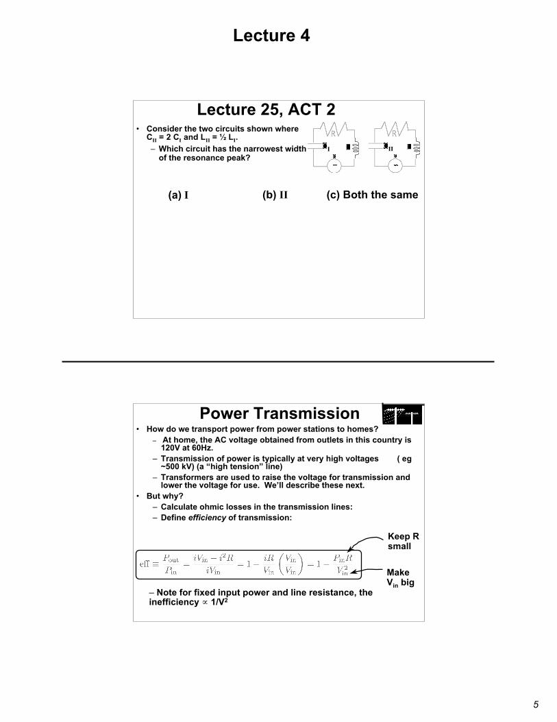
Power Transmission• How do we transport power from power stations to homes?
– At home, the AC voltage obtained from outlets in this country is120V at 60Hz.
– Transmission of power is typically at very high voltages ( eg~500 kV) (a “high tension” line)
– Transformers are used to raise the voltage for transmission andlower the voltage for use. We’ll describe these next.
• But why?– Calculate ohmic losses in the transmission lines:– Define efficiency of transmission:
– Note for fixed input power and line resistance, theinefficiency ∝ 1/V2
Keep Rsmall
MakeVin big

6
Lecture 4
Transformers
∼ε
(primary) (secondary)
• AC voltages can be stepped upor stepped down by the use oftransformers.
iron
• The AC current in the primarycircuit creates a time-varyingmagnetic field in the iron
• The iron is used to maximize the mutual inductance. Weassume that the entire flux produced by each turn of theprimary is trapped in the iron.
V2V1
• This induces an emf on thesecondary windings due to themutual inductance of the two setsof coils.
Ideal Transformers (no load)
• The primary circuit is just an AC voltagesource in series with an inductor. The changein flux produced in each turn is given by:
• The change in flux per turn in the secondary coil is thesame as the change in flux per turn in the primary coil(ideal case). The induced voltage appearing across thesecondary coil is given by:
• Therefore,• N2 > N1 ⇒ secondary V2 is larger than primary V1 (step-up)• N1 > N2 ⇒ secondary V2 is smaller than primary V1 (step-down)
• Note: “no load” means no current in secondary. The primary current,termed “the magnetizing current” is small!
No resistance losses All flux contained in iron Nothing connected on secondary

7
Lecture 4
Ideal Transformers• What happens when we connect a
resistive load to the secondary coil?– Flux produced by primary coil induces
an emf in secondaryR
with a Load
– This changing flux appears in theprimary circuit as well; the sense of itis to reduce the emf in the primary...
– However, V1 is a voltage source.– Therefore, there must be an increased
current i1 (supplied by the voltagesource) in the primary which producesa flux ∝ N1i1 which exactly cancels theflux produced by i2.
– emf in secondary produces current i2
– This current produces a flux in thesecondary coil ∝ N2i2, which opposesthe original flux -- Lenz’s law
Transformers with a Load• With a resistive load in the secondary,
the primary current is given by:R
It’s time..

8
Lecture 4
Lecture 25, ACT 3• The primary coil of an ideal transformer is
connected to a battery (V1 = 12V) as shown.The secondary winding has a load of 2 Ω.There are 50 turns in the primary and 200turns in the secondary.
R
– What is the current in the secondcary ?
ε
N2N1(primary) (secondary)
iron
V2V1
(a) 24 A (b) 1.5 A (c) 6 A (d) 0 A
Lecture 25, ACT 4• The primary coil of an ideal transformer is
connected to the wall (V1 = 120V) as shown.There are 50 turns in the primary and 200turns in the secondary.
R
– If 960 W are dissipated in the resistorR, what is the current in the primary ?
(a) 8 A (b) 16 A (c) 32 A

9
Lecture 4
Fields from Circuits?• We have been focusing on what happens within the circuits we have
been studying (eg currents, voltages, etc.)
• What’s happening outside the circuits??– We know that:
» charges create electric fields and» moving charges (currents) create magnetic fields.
– Can we detect these fields?– Demos:
» We saw a bulb connected to a loop glow when the loop camenear a solenoidal magnet.
» Light spreads out and makes interference patterns.Do we understand this?
f( )x
x
f( x
x
z
y

10
Lecture 4
Maxwell’s Equations• These equations describe all of Electricity and
Magnetism.
• They are consistent with modern ideas such asrelativity.
• They describe light !
Maxwell’s Equations - Revised• In free space, outside the wires of a circuit, Maxwell’s equations
reduce to the following.
• These can be solved (see notes) to give the followingdifferential equations for E and B.
• These are wave equations. Just like for waves on astring. But here the field is changing instead of thedisplacement of the string.

11
Lecture 4
Step 1 Assume we have a plane wave propagating in z (ie E, Bnot functions of x or y)
Plane Wave Derivation
x
z
y
z1 z2
Ex Ex
ΔZ
Δx
By
Step 2 Apply Faraday’s Law to infinitesimal loop in x-z plane
Example: does this
Plane Wave Derivation
x
z
y
z1 z2
By
ΔZ
ΔyBy
Ex
Step 3 Apply Ampere’s Law to an infinitesimal loop in the y-zplane:
Step 4 Combine results from steps 2 and 3 to eliminate By
!!

12
Lecture 4
Plane Wave Derivation• We derived the wave eqn for Ex:
• By is in phase with Ex• B0 = E0 / c
• How are Ex and By related in phase and magnitude?
(Result from step 2)
• We could have also derived for By:
– Consider the harmonic solution: where
Review of Waves from last semester• The one-dimensional wave equation:
• A specific solution for harmonic waves traveling in the +xdirection is:
has a general solution of the form:
where h1 represents a wave traveling in the +x direction and h2represents a wave traveling in the -x direction.
h
x
λA
A = amplitudeλ = wavelengthf = frequencyv = speedk = wave number

13
Lecture 4
E & B in Electromagnetic Wave• Plane Harmonic Wave:
where:
y
x
z
Nothing special about (Ey,Bz); eg could have (Ey,-Bx)
Note: the direction of propagation is given by the cross product
where are the unit vectors in the (E,B) directions.
Note cyclical relation:
Lecture 25, ACT 5• Suppose the electric field in an e-m wave is given by:
– In what direction is this wave traveling ?5A
(a) + z direction (b) -z direction(c) +y direction (d) -y direction

14
Lecture 4
Lecture 25, ACT 5• Suppose the electric field in an e-m wave is given
by:
• Which of the following expressions describesthe magnetic field associated with this wave?(a) Bx = -(Eo/c)cos(kz + ωt) (b) Bx = +(Eo/c)cos(kz - ωt) (c) Bx = +(Eo/c)sin(kz - ωt)
5B
Velocity of Electromagnetic Waves• The wave equation for Ex: (derived from Maxwell’s Eqn)
• Therefore, we now know the velocity ofelectromagnetic waves in free space:
• Putting in the measured values for µ0 & ε0, we get:
• This value is identical to the measured speed of light!– We identify light as an electromagnetic wave.

15
Lecture 4
The EM Spectrum
• These EM waves can take on any wavelength fromangstroms to miles (and beyond).
• We give these waves different names depending on thewavelength.
Wavelength [m]10-14 10-10 10-6 10-2 1 102 106 1010
Gam
ma
Ray
s
Infr
ared
Mic
row
aves
Shor
t Wav
e R
adio
TV a
nd F
M R
adio
AM
Rad
io
Long
Rad
io W
aves
Ultr
avio
let
Visi
ble
Ligh
t
X R
ays
Energy in EM Waves / review• Electromagnetic waves contain energy which is stored in E
and B fields:
• The Intensity of a wave is defined as the average powertransmitted per unit area = average energy density times wavevelocity:
• Therefore, the total energy density in an e-m wave = u, where
=
Related Documents