PHYSICAL REVIEW D 044036 (2011) Reconstructing the …pubman.mpdl.mpg.de/pubman/item/escidoc:1313725/component/esci… · Reconstructing the massive black hole cosmic history through

Reconstructing the massive black hole cosmic history through gravitational waves

Alberto Sesana,1,* Jonathan Gair,2,† Emanuele Berti,3,4,‡ and Marta Volonteri5,x1Albert Einstein Institute, Am Muhlenberg 1 D-14476 Golm, Germany

2Institute of Astronomy, University of Cambridge, Cambridge, CB3 0HA, UK3Department of Physics and Astronomy, The University of Mississippi, University, Mississippi 38677-1848, USA

4California Institute of Technology, Pasadena, California 91109, USA5Department of Astronomy, University of Michigan, Ann Arbor, Michigan, USA

(Received 17 November 2010; published 22 February 2011)

The massive black holes we observe in galaxies today are the natural end-product of a complex

evolutionary path, in which black holes seeded in proto-galaxies at high redshift grow through cosmic

history via a sequence of mergers and accretion episodes. Electromagnetic observations probe a small

subset of the population of massive black holes (namely, those that are active or those that are very close to

us), but planned space-based gravitational wave observatories such as the Laser Interferometer Space

Antenna (LISA) can measure the parameters of ‘‘electromagnetically invisible’’ massive black holes out

to high redshift. In this paper we introduce a Bayesian framework to analyze the information that can be

gathered from a set of such measurements. Our goal is to connect a set of massive black hole binary

merger observations to the underlying model of massive black hole formation. In other words, given a set

of observed massive black hole coalescences, we assess what information can be extracted about the

underlying massive black hole population model. For concreteness we consider ten specific models of

massive black hole formation, chosen to probe four important (and largely unconstrained) aspects of the

input physics used in structure formation simulations: seed formation, metallicity ‘‘feedback’’, accretion

efficiency and accretion geometry. For the first time we allow for the possibility of ‘‘model mixing’’, by

drawing the observed population from some combination of the ‘‘pure’’ models that have been simulated.

A Bayesian analysis allows us to recover a posterior probability distribution for the ‘‘mixing parameters’’

that characterize the fractions of each model represented in the observed distribution. Our work shows that

LISA has enormous potential to probe the underlying physics of structure formation.

DOI: 10.1103/PhysRevD.83.044036 PACS numbers: 04.30.Tv, 04.30.w, 04.70.s, 97.60.Lf

I. INTRODUCTION

In CDM cosmologies, structure formation proceeds ina hierarchical fashion [1], in which massive galaxies arethe result of several merging events involving smallerbuilding blocks. In this framework, the massive black holes(MBHs) we see in today’s galaxies are expected to be thenatural end-product of a complex evolutionary path, inwhich black holes seeded in proto-galaxies at high redshiftgrow through cosmic history via a sequence of MBH-MBHmergers and accretion episodes [2,3]. Hierarchical modelsfor MBH evolution, associating quasar activity to gas-fueled accretion following galaxy mergers, have been suc-cessful in reproducing several properties of the observedUniverse, such as the present-day mass density of nuclearMBHs and the optical and X-ray luminosity functions ofquasars [3–9].

However, only a few percent of galaxies host a quasaror an active galactic nucleus (AGN), while most galaxiesharbor MBHs in their centers, as exemplified by

stellar- and gas-dynamical measurements that led to thediscovery of quiescent MBHs in almost all bright nearbygalaxies [10], including the Milky Way [11]. Our currentknowledge of the MBH population is therefore limitedto a small fraction of MBHs: either those that are active,or those in our neighborhood, where stellar- and gas-dynamical measurements are possible. Gravitationalwave (GW) observatories can reveal the population ofelectromagnetically ‘‘black’’ MBHs.LISA will be capable of accurately measuring the pa-

rameters of individual massive black hole binaries(MBHBs), such as their masses and luminosity distance,allowing us to track the merger history of the MBH popu-lation out to large redshifts. MBHB mergers have been oneof the main targets of the LISA mission since its concep-tion (see e.g. [12]). Several authors have explored howspins, higher harmonics in the GW signal and eccentricityaffect parameter estimation and, in particular, source lo-calization, which is fundamental to search for electro-magnetic counterparts (see, for example, the work by theLISA parameter estimation task force [13] and referencestherein). Most work on parameter estimation has focusedon inspiral waveforms, but ringdown observations can alsoprovide precise measurements of the parameters of rem-nant MBHs resulting from a merger, and even test the Kerr

*[email protected]†[email protected]‡[email protected]@umich.edu

PHYSICAL REVIEW D 83, 044036 (2011)

1550-7998=2011=83(4)=044036(26) 044036-1 2011 American Physical Society

http://dx.doi.org/10.1103/PhysRevD.83.044036

nature of astrophysical MBHs [14]. Initial studies usingnumerical relativity waveforms suggest that mergers willimprove the signal-to-noise ratio of individual events andthe localization accuracy of LISA [15].

While highly precise measurements for individual sys-tems are interesting and potentially very useful for makingstrong-field tests of general relativity, it is the properties ofthe set of MBHB mergers that are observed which willcarry the most information for astrophysics. To date, mostof the body of work considering observations of more thanone MBHB system has focused on the use of MBHBs as‘‘standard sirens’’ [16] to probe the expansion history ofthe Universe. For a subset of the observed binaries, LISAmay have sufficient angular resolution to make follow-upelectromagnetic observations feasible. If the host galaxy orgalaxy cluster can be identified, this will allow LISA tomeasure the dark energy equation of state to levels com-parable to those expected from other dark energy missions[17]. The effectiveness of LISA as a dark energy probe islimited by weak-lensing [18], but this can be mitigated tosome extent [19], and a combination of several GW detec-tions may still provide useful constraints on the darkenergy equation of state [20].

GWobservations of multiple MBHB mergers could alsobe combined to extract useful astrophysical informationabout their formation and evolution through cosmic his-tory. As already mentioned, our access to the MBH popu-lation in the Universe is limited to AGNs or to quiescentMBHs in nearby galaxies. In this sense we are probing onlythe tip of the iceberg. Theoretical astrophysicists havedeveloped a large variety of MBH formation models[3,21–24] that are compatible with observational con-straints. However, the natural lack of observations of faintobjects at high redshifts and the difficulties in measuringMBH spins leave a lot of freedom in modeling MBH seedformation and mass accretion. In the last decade, severalauthors have employed different MBH formation and evo-lution models to make predictions for future GW observa-tions, focusing, in particular, on LISA [25–30]. This efforthas been very valuable, and established the detection of alarge population of MBH binaries as one of the corner-stones of the LISA mission.

In this paper we tackle the inverse problem: we do notask what astrophysics can do for LISA, but what LISA cando for astrophysics. In particular, we ask the followingquestion: can we discriminate among different MBH for-mation and evolution scenarios on the basis of GW obser-vations only? More ambitiously, given a set of observedMBHB coalescences, what information can be extractedabout the underlying MBH population model? For ex-ample, will GW observations tell us something about themass spectrum of the seed black holes at high redshift thatare inaccessible to conventional electromagnetic observa-tions, or about the poorly understood physics of accretion?Such information cannot be gleaned from a single GW

observation, but it is encoded in the collective properties ofthe whole detected sample of coalescing binaries. In thispaper we describe a method to extract this information inorder to make meaningful astrophysical statements. Themethod is based on a Bayesian framework, using a para-metric model for the probability distribution of observedevents.The paper is organized as follows. Section II presents the

general framework of our analysis. There we review theMBH formation models considered in this paper andexplain how these models translate into a theoreticallyobservable distribution via a ‘‘transfer function’’ that de-pends (for a given source) on the detector characteristicsand on the assumed model for the gravitational wave-form. We describe how to sample MBH distributions viaMonte Carlo methods, and how to interpret the observa-tions in a Bayesian framework. In Sec. III we apply thesestatistical methods to the problem of deciding, given a setof LISA observations, whether we can correctly tell thetrue model from an alternative, for each pair in our familyof MBH formation models. We focus, in particular, onspecific comparisons that would allow us to set constraintson the main uncertainties in the input physics; namely, theseed formation mechanism, the redshift distribution of thefirst seeds, the efficiency of accretion during each mergerand the geometry of accretion. In Sec. IV we describe howto go beyond a simple catalog of pure models, either byintroducing phenomenological mixing parameters (de-signed to gauge the relative importance of different physi-cal mechanisms in the birth and growth of MBHs) betweenthe pure models, or by consistently implementing a mix-ture of different physical assumptions in a merger treesimulation. In Sec. V we explore how well a ‘‘consistentlymixed’’ model can be recovered as a superposition ofpure models with the phenomenological mixing parame-ters. In the conclusions we point out possible extensions ofour work. Appendix A provides details of our treatment oferrors (due to instrumental noise, uncertainties in cosmo-logical parameters and weak-lensing) in the MBHB obser-vations. Appendix B compares parameter estimationcalculations that do, or do not, take into account the orbitalmotion of LISA. The results suggest that angle-averagedcodes that do not take into account the orbital motion mayreduce computational requirements in Monte Carlo simu-lations, while still providing reasonable estimates of atleast some binary parameters. Finally, Appendix C givesdetails on the assumptions underlying the black hole for-mation models used in this paper, and, in particular, onmetallicity evolution, seeding and accretion.

II. MASSIVE BLACK HOLES: FORMATIONMODELS, GRAVITATIONALWAVE

OBSERVATIONS AND THEIR INTERPRETATION

Our goal is to assess the effectiveness of GW observa-tions in extracting useful information about the evolution

SESANA et al. PHYSICAL REVIEW D 83, 044036 (2011)

044036-2

of the MBH population in the Universe. Recent work byPlowman et al. [31,32] attempted to address the samequestion. Here we use different techniques, which improveon their analysis in several ways. Plowman et al. used thenonparametric Kolmogorov-Smirnov (KS) test to comparedistributions of model parameters between models. Thislimited their comparisons to two parameters at a time, ashigher-dimensional KS tests are not known. We instead usea parametric model by considering the number of events inany given part of parameter space to be drawn from aPoisson probability distribution. This allows us to use aBayesian framework for the analysis. Such a frameworkwill be important for the analysis of the actual LISAobservations once these have been made, and it can beapplied to a parameter space of any dimension.

In Ref. [33] we used similar techniques to compare thesame four models that were considered by Plowman et al.,which were the models used for LISA parameter estima-tion accuracy studies in Ref. [13]. In this paper we goconsiderably further by considering six additional models,chosen to probe four key aspects of the input physics usedin structure formation simulations: seed formation, metal-licity ‘‘feedback’’, accretion efficiency and accretiongeometry. In addition, we consider for the first time‘‘model mixing’’. The idea is to assume that the observedpopulation is drawn from some combination of the ‘‘pure’’models that have been simulated. The Bayesian frameworkallows us to recover a posterior probability distribution forthe ‘‘mixing parameters’’ that characterize the fraction ofeach model represented in the observed distribution. Suchan analysis is not possible in the KS framework. The modelmixing analysis is very important, as the real Universe ismost certainly not drawn from any of the idealized modelsthat currently exist. The mixing parameters will reflect therelative contributions in the true Universe of the differentinput physics in the pure models.

For our analysis, we adopt the following strategy:(i) We consider a set of MBH formation and evolution

models predicting different coalescing MBHB theo-retical distributions (Sec. II A);

(ii) To account for detection incompleteness, we filterthe distribution predicted by each model using adetector ‘‘transfer function’’ that produces the ob-served theoretical distributions under some specificassumptions about the GW detector (Sec. II B). Thisis basically the distribution one would observe as-suming an infinite number of detections;

(iii) We generate Monte Carlo realizations of the co-alescing MBHB population from one of the models(Sec. II C) or from a mixture of models (Sec. IV),and simulate GW observations of the inspiralingbinaries, including errors in the source parameterestimation;

(iv) We then compare (in a statistical sense) the catalogof observed events—including measurement

errors—with the observed theoretical distributions,to assess at what level of confidence we can recoverthe parent model. The statistical methods we useare detailed in Sec. II D.

In this paper we will consider the Laser InterferometerSpace Antenna (LISA) as an illustrative case, but thestrategy outlined above can easily be generalized to otherproposed space-borne GW observatories, such as ALIA,DECIGO or BBO [34–36].An important caveat is that, for a source at redshift z,

GW observations do not measure the binary parameters inthe source frame, but rather the corresponding redshiftedquantities in the detector frame. For this reason, throughoutthe paper we shall characterize MBHBs via their redshiftedparameters. Given a MBHB with rest-frame massesM1;r > M2;r, the masses in the detector frame are given

byM1 ¼ ð1þ zÞM1;r,M2 ¼ ð1þ zÞM2;r. In terms of these

masses we can also define (as is the custom in GW physics)the total massM ¼ M1 þM2, the mass ratio q ¼ M2=M1,the symmetric mass ratio ¼ M1M2=M

2 and the chirp

mass M ¼ 3=5M. In our calculations we assume aconcordance CDM cosmology characterized by H0 ¼70 km s1 Mpc1, M ¼ 0:27 and ¼ 0:73.For simplicity we will focus on the inspiral of circular,

nonspinning binaries; therefore, each coalescing MBHB inour populations will be characterized by only three intrin-sic parameters (z, M and q). In terms of gravitationalwaveform modelling, the results presented here can beconsidered conservative. Different accretion models mayresult in different MBH spin distributions. Including spinin the analysis will provide additional information that willhelp to further constrain the physical mechanisms at workin shaping the MBH population model [32,37]. The inclu-sion of the merger/ringdown portion of the signal willincrease the signal-to-noise ratio (SNR) of observed bi-naries and allow measurements of the parameters of themerger remnants, providing additional information on themechanisms responsible for MBH growth.In the following subsections we will introduce all the

elements and methodologies relevant to our analysis.

A. Cosmological massive black hole populations

The assembly of MBHs is reconstructed through dedi-cated Monte Carlo merger tree simulations [3] which areframed in the hierarchical structure formation paradigm.Each model is constructed by tracing the merger hierarchyof200 dark matter halos in the mass range 1011–1015Mbackwards to z ¼ 20, using an extended Press & Schechter(EPS) algorithm (see [3] for details). The halos are thenseeded with black holes and their evolution is trackedforward to the present time. Following a major merger(defined as a merger between two halos with mass ratioMh2=Mh1 > 0:1, whereMh2 is the mass of the lighter halo),

MBHs accrete efficiently an amount of mass that scales

RECONSTRUCTING THE MASSIVE BLACK HOLE COSMIC . . . PHYSICAL REVIEW D 83, 044036 (2011)

044036-3

with the fifth power of the host halo circular velocity and

that is normalized to reproduce the observed local corre-

lation between MBH mass and the bulge stellar velocity

dispersion (the M relation, see [38] and references

therein). For each of the simulated halos, all of the binary

coalescences that occur are stored in a catalog. The results

for each halo are then weighted using the EPS halo mass

function and are numerically integrated over the observ-

able volume shell at every redshift to obtain the coales-

cence rate of MBHBs as a function of black hole masses

and redshift (see, e.g., Fig. 1 in [28]). We then find the

theoretical distribution of (potentially) observable coales-

cing binaries by multiplying the rate by the LISA mission

lifetime (here assumed to be three years) to obtain the

distribution N i d3Ni=dzdMdq, where the index ilabels the MBH formation model.

In the general picture of MBH cosmic evolution, the

MBH population is shaped by the details of the seeding

process and the accretion history. Both issues are poorly

understood, and largely unconstrained by present observa-

tions. We identify four key factors that have a direct impact

on specific observable properties of the merging MBHB

population:(1) the seed formation mechanism shapes the initial

seed mass function;(2) the impact of metallicity on MBH formation deter-

mines the redshift distribution of the seeds;(3) the accretion efficiency determines the growth rate

of MBHs over cosmic history;(4) the accretion geometry is crucial in the evolution of

the MBH spins.

We explore different formation scenarios by considering

two different prescriptions for each of the elements in

the above list. Details of the implementation are described

in Appendix C, here we summarize the most impor-

tant assumptions, and differences between models, as fol-

lows:(1) The seed formation mechanism. Two distinct fami-

lies of models have become popular in the lastdecade, usually referred to as ‘‘light’’ and ‘‘heavy’’seed models. Here we consider two different scenar-ios representative of the two possibilities. (i) The‘‘VHM’’ model; developed by Volonteri, Haardt &Madau [3], this model is characterized by light seeds(M 100M), which are thought to be the remnantsof Population III (POPIII) stars, the first generationof stars in the Universe [39]. (ii) The ‘‘BVR’’model;proposed by Begelman, Volonteri & Rees [23], thismodel belongs to the family of ‘‘heavy seed’’ mod-els. Bar within bar instabilities [40] occurring inmassive protogalactic disks trigger gas inflow to-ward the center, where a ‘‘quasistar’’ forms. Thecore of the quasistar collapses into a seed black holethat efficiently accretes from the quasistar envelope,

resulting in a final seed black hole with massM few 104M.

(2) Metallicity ‘‘feedback’’. Both of the black hole for-mation models described above require that a largeamount of gas is efficiently transported to the halocenter. The gas inflow has to occur on a time scalethat is shorter than that of star formation, to avoidcompetition in gas consumption and disruption ofthe inflow process by supernovae explosions. It hasbeen suggested that metal-free conditions are con-ducive to efficient gas inflow, as fragmentation isinhibited [41]. If fragmentation is suppressed, andcooling proceeds gradually, the gaseous componentcan cool and contract before many stars form. Thegas metallicity Z is therefore an important environ-mental factor to take into account, and we considertwo cases. (i) ‘‘noZ’’ models; black hole seeding isassumed to be efficient at zero-metallicity only, witha sharp threshold in cosmic time. In these models,seeds form at very high redshift (20> z > 15).(ii) ‘‘Z’’ models; efficient seed formation occursalso at later times. Here we treat POPIII star andquasistar black hole formation differently. We stillassume that POPIII stars can form only out of metal-free gas, but we track the probability that a halo atlate times is still metal-free by adopting the metalenrichment models developed in [42]. For the caseof quasistars, instead, we drop the assumption ofzero-metallicity. This choice is motivated by recenthigh-resolution numerical simulations of gas-richgalaxies at solar metallicities (e.g. [43]), whichshow that bar within bar instabilities can drive asignificant amount of gas to the central nucleusbefore star formation quenches the inflow. Thesemodels are characterized by seed formation also atlater times, in metal enriched halos. See [24] for fulldetails on the model and its implementation.

(3) The accretion efficiency. MBHs powering AGNsexhibit a broad phenomenology; they accrete atdifferent rates, with different efficiencies and lumi-nosities (see [44] and references therein). In theabsence of a solid coherent theory for describingthe accretion process, several toy models are viable,and we consider two of these models. (i) ‘‘Edd’’accretion model; the easiest possible recipe is toassume that accretion occurs at the Eddington rate,parametrized through the Eddington ratio fe (wetake fe ¼ 0:3 in our models). (ii) ‘‘MH’’ accretionmodel; we also use a more sophisticated schemecombining low and high accretion rates, as de-scribed by Merloni & Heinz [44].

(4) The geometry of accretion. Standard accretion disksare unstable to self-gravity beyond a few thousandsof Schwarzschild radii [45]. It is therefore not guar-anteed that the supply of gas to the central black


044036-4

hole will be continuous, smooth and planar. Weconsider two different scenarios. (i) Coherent accre-tion (‘‘co’’ models); the flow of material that feedsthe black hole is assumed to be continuous, smoothand planar. Accretion is a single steady episodelasting about a Salpeter time. (ii) Chaotic accretion(‘‘ch’’models); in this scenario, proposed by King &Pringle [46], a single accretion event is made of acollection of short-lived accretion episodes, and theangular momentum of each accreted matter clump israndomly oriented. These accretion models primar-ily lead to different expectations for the black holespins: intermediate-high, a 0:6–0:9, in the coher-ent case; low, a < 0:2, in the chaotic case [37]. Inthis work we ignore black hole spin in the modelingof gravitational waveforms, and therefore we do notassess the impact of spin measurements in resolvingdifferent MBH formation scenarios. However, theaccretion prescription also leaves an imprint onthe component masses. The models assume thatthe mass-to-energy conversion efficiency, , de-pends on black hole spin only, so the two modelspredict different average efficiencies of 20% and10%, respectively. The mass-to-energy conver-sion directly affects mass growth, with high effi-ciency implying slow growth, since for a black holeaccreting at the Eddington rate the black hole massincreases with time as

MðtÞ ¼ Mð0Þ exp1

t

tEdd

; (1)

where tEdd ¼ 0:45 Gyr. The ‘‘coherent’’ versus‘‘chaotic’’ models thus allow us to study how differ-ent growth rates affect LISA observations.

By choosing two different prescriptions for each of thefour pieces of input physics listed above we built tendifferent MBH population models, which are summarizedin Table I. We shall refer to these models as ‘‘pure’’, in thesense that we do not mix different recipes for seed

formation and accretion history (e.g., accretion is eithercoherent or chaotic, etc.). We will consider ‘‘mixed’’ mod-els in Sec. IV. It is worth emphasizing that all of thesemodels successfully reproduce various properties of theobserved Universe, such as the present-day mass densityof nuclear MBHs and the optical and X-ray luminosityfunctions of quasars. GW observations may therefore pro-vide an invaluable tool to constrain the birth and growth ofMBHs, particularly at high redshift.

B. Theoretically observable distributions:the transfer function

In order to compare a set of observed events to a givenMBH population model, we must map the coalescencedistribution predicted by the model to a theoretically ob-servable distribution which takes into account the ‘‘incom-pleteness’’ of the observations resulting from the limitedsensitivity of any given GW detector. This information canbe encoded in a transfer function Tðz;M; qÞ, that dependsonly on the detector characteristics and on the gravitationalwaveform model.We model the detector and the gravitational waveform

following Refs. [47,48]. The detector response is modeledfollowing Cutler [49]: the three-arm LISA constellation isthought of as a superposition of a pair of linearly indepen-dent two-arm right-angle interferometers, and we can es-timate the effect of ‘‘descoping options’’ or a failure on onesatellite by assuming that only one of the two detectors isoperational. The MBHB inspiral signal is modeled usingthe restricted post-Newtonian approximation, truncatingthe GW phasing at second post-Newtonian order—i.e., atorder ðv=cÞ4, where v is the binary orbital velocity. We alsolimit our analysis to circular inspirals of nonspinningMBHs and neglect contributions to the observable signalthat come from higher harmonics in the inspiral signal andfrom the (gravitationally loud) merger/ringdown phase.The latter assumption significantly underestimates the en-ergy carried in the GWs [50], the SNR of the signal [51]and the accuracy in estimating the source parameters [15].

TABLE I. The ten ‘‘pure’’ MBH population models considered in this paper. For convenience,in the following we will identify models by the integer, i, listed in the second column. In the lastcolumn, Ni denotes the predicted coalescence rate.

Name i Seeding Metallicity Accretion model Accretion geometry Ni [yr1]

VHM-noZ-Edd-co 1 POPIII Z ¼ 0 Eddington coherent 86

VHM-noZ-Edd-ch 2 POPIII Z ¼ 0 Eddington chaotic 81

VHM-Z-Edd-co 3 POPIII all Z Eddington coherent 108

VHM-Z-Edd-ch 4 POPIII all Z Eddington chaotic 113

BVR-noZ-Edd-co 5 Quasistar Z ¼ 0 Eddington coherent 26

BVR-noZ-Edd-ch 6 Quasistar Z ¼ 0 Eddington chaotic 24

BVR-Z-Edd-co 7 Quasistar all Z Eddington coherent 22

BVR-Z-Edd-ch 8 Quasistar all Z Eddington chaotic 29

BVR-noZ-MH-co 9 Quasistar Z ¼ 0 Merloni & Heinz coherent 33

BVR-noZ-MH-ch 10 Quasistar Z ¼ 0 Merloni & Heinz chaotic 33


044036-5

From the point of view of studying MBH populations, italso means that we discard all information on the mass andspin distribution of MBHs formed as a result of eachmerger [14]. In this sense, our assessment of the potentialof LISA to constrain MBH formation models should beconsidered conservative.

An important advantage of working in the frequencydomain and of adopting a simplified waveform model isthat we can sample the three-dimensional space ðz;M; qÞby fast Monte Carlo simulations using an adaptation of theFORTRAN code described in [47]. Typically, we can esti-

mate SNRs and parameter estimation errors of 106 bi-naries in 1 d on a single processor. This would not bepossible with a more complex time-domain code includingspin dynamics, such as that used in [32]. We consider a21 21 21 three-dimensional grid spaced logarithmi-cally in the intervals q 2 ½103; 1, M 2 ½103; 108, andapproximately linearly in z (namely, we consider z ¼ 0:5and then all values of z ¼ 1; . . . ; 20 in steps ofz ¼ 1), fora total of 9261 points. At each point, we generate 1000binaries assuming random position in the sky and orienta-tion, random phase at coalescence, and coalescence time tcin the range [0, 3 yr] (i.e., we consider only events thatcoalesce during the LISA mission). The GW signal iscalculated in the Fourier domain in the stationary phaseapproximation. Our statistical analysis, which will be dis-cussed in Sec. II D, includes parameter measurement er-rors, which are modeled as described in Appendix A. Themodeling of errors due to instrumental noise relies on thecomputation of the so-called Fisher information matrix[52]. For each system we compute the Fisher matrix andits inverse by means of the LU decomposition, as describedin [47]. The accuracy of the inversion is usually worse forcertain values of the intrinsic parameters and of the angularposition/orientation of the binary. We discard ‘‘bad’’ Fishermatrix inversions by monitoring a quantity inv, defined as

inv ¼ maxi;j

jInumij ijj; (2)

where Inumij is the ‘‘numerical’’ identity matrix obtained by

multiplying the inverse matrix by the original, and ij is

the standard Kronecker delta symbol [47]. We set a maxi-mum tolerance of inv ¼ 103 to accept the inversion. Forthe accepted events, we compute the SNR and then wedefine the transfer function as

Tðz;M; qÞ ¼ Nð > thrÞN

; (3)

where N ¼ 1000 is the number of successful matrix inver-sions at any given grid point and Nð > thrÞ is the numberof binaries fulfilling the condition > thr, where thr is aprespecified SNR threshold.

We consider four transfer functions Tjðz;M; qÞ (j ¼ 1,

2, 3, 4) according to the following prescriptions: (1) oneinterferometer, thr ¼ 8; (2) one interferometer, thr ¼ 20;(3) two interferometers, thr ¼ 8; (4) two interferometers,

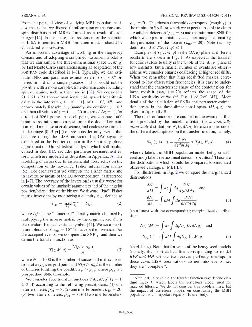
thr ¼ 20. The chosen thresholds correspond (roughly) tothe minimum SNR for which we expect to be able to claima confident detection (thr ¼ 8) and the minimum SNR forwhich we expect to obtain a decent accuracy in estimatingthe parameters of the source (thr ¼ 20). Note that, bydefinition, 0 Tðz;M; qÞ 1.Examples of T3ðz;M; qÞ in the ðM;qÞ plane at different

redshifts are shown in Fig. 1. As expected, the transferfunction is close to unity in the whole of the ðM;qÞ plane atlow redshifts, but a smaller number of events are observ-able as we consider binaries coalescing at higher redshifts.When we remember that high redshifted masses corre-spond to low observation frequencies, it is easy to under-stand that the characteristic shape of the contour plots forlarge redshift (say, z ¼ 20) reflects the shape of theLISA sensitivity curve (cf. Fig. 1 of Ref. [47]). Moredetails of the calculation of SNRs and parameter estima-tion errors in the three-dimensional space ðM;q; zÞ aregiven in Appendix B.The transfer functions are coupled to the event distribu-

tions predicted by the models to obtain the theoreticallyobservable distributions NTðz;M; qÞ for each model underthe different assumptions on the transfer function; namely,

NTi;jðz;M; qÞ ¼ d3Ni

dzdMdq Tjðz;M; qÞ; (4)

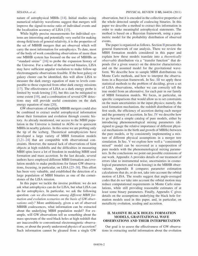
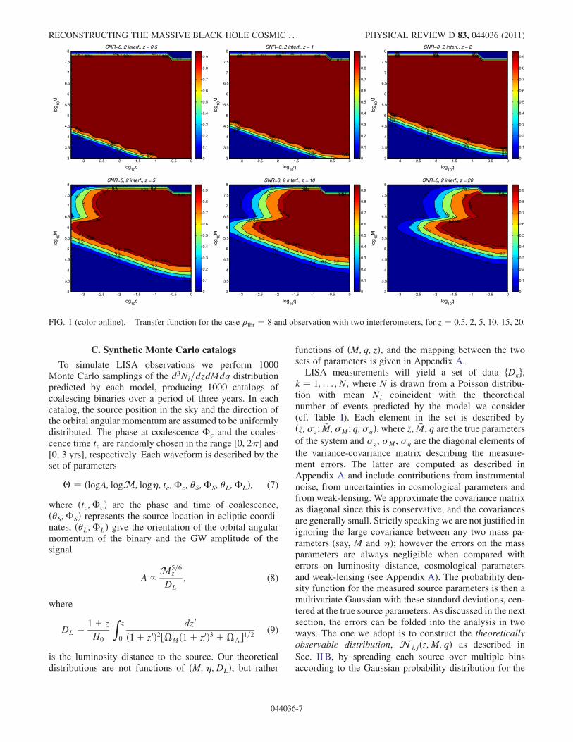
where i labels the MBH population model being consid-ered and j labels the assumed detector specifics.1 These arethe distributions which should be compared to simulatedobserved catalogs of MBHBs.For illustration, in Fig. 2 we compare the marginalized

distributions

dNi

dM¼

Zdz

Zdq

d3Ni

dzdMdqand

dNi

dz¼

ZdM

Zdq

d3Ni

dzdMdq(5)

(thin lines) with the corresponding marginalized distribu-tions

NTi;3ðMÞ ¼

Zdz

ZdqNTi;3

ðz;M; qÞ and

NTi;3ðzÞ ¼

ZdM

ZdqNTi;3

ðz;M; qÞ (6)

(thick lines). Note that for some of the heavy seed models(namely, the short-dashed line corresponding to modelBVR-noZ-MH-co) the two curves perfectly overlap: inthese cases LISA observations do not miss events, i.e.they are ‘‘complete’’.

1Note that, in principle, the transfer function may depend on athird index k, which labels the waveform model used formatched filtering. We do not consider this problem here, butthe impact of waveform models on constraining the MBHpopulation is an important topic for future study.


044036-6

C. Synthetic Monte Carlo catalogs

To simulate LISA observations we perform 1000Monte Carlo samplings of the d3Ni=dzdMdq distributionpredicted by each model, producing 1000 catalogs ofcoalescing binaries over a period of three years. In eachcatalog, the source position in the sky and the direction ofthe orbital angular momentum are assumed to be uniformlydistributed. The phase at coalescence c and the coales-cence time tc are randomly chosen in the range [0, 2] and[0, 3 yrs], respectively. Each waveform is described by theset of parameters

¼ ðlogA; logM; log; tc;c; S;S; L;LÞ; (7)

where ðtc;cÞ are the phase and time of coalescence,ðS;SÞ represents the source location in ecliptic coordi-nates, ðL;LÞ give the orientation of the orbital angularmomentum of the binary and the GW amplitude of thesignal

A / M5=6z

DL

; (8)

where

DL ¼ 1þ z

H0

Z z

0

dz0

ð1þ z0Þ2½Mð1þ z0Þ3 þ1=2(9)

is the luminosity distance to the source. Our theoreticaldistributions are not functions of ðM;;DLÞ, but rather

functions of ðM;q; zÞ, and the mapping between the twosets of parameters is given in Appendix A.LISA measurements will yield a set of data fDkg,

k ¼ 1; . . . ; N, where N is drawn from a Poisson distribu-tion with mean Ni coincident with the theoreticalnumber of events predicted by the model we consider(cf. Table I). Each element in the set is described byðz; z; M;M; q;qÞ, where z, M, q are the true parameters

of the system and z, M, q are the diagonal elements of

the variance-covariance matrix describing the measure-ment errors. The latter are computed as described inAppendix A and include contributions from instrumentalnoise, from uncertainties in cosmological parameters andfrom weak-lensing. We approximate the covariance matrixas diagonal since this is conservative, and the covariancesare generally small. Strictly speaking we are not justified inignoring the large covariance between any two mass pa-rameters (say, M and ); however the errors on the massparameters are always negligible when compared witherrors on luminosity distance, cosmological parametersand weak-lensing (see Appendix A). The probability den-sity function for the measured source parameters is then amultivariate Gaussian with these standard deviations, cen-tered at the true source parameters. As discussed in the nextsection, the errors can be folded into the analysis in twoways. The one we adopt is to construct the theoreticallyobservable distribution, N i;jðz;M; qÞ as described in

Sec. II B, by spreading each source over multiple binsaccording to the Gaussian probability distribution for the

1.01.00.1

0.1

0.1

0.3 0.30.3

0.3

0.3

0.5 5.05.0

0.5

0.7 0.7 0.7

0.7

0.7

0.7

9.09.09.0

0.9

0.9

0.9

0.95 0.95 0.95

0.95

0.95

0.95

log10

q

log 10

M

SNR=8, 2 interf., z = 0.5

−3 −2.5 −2 −1.5 −1 −0.5 03

3.5

4

4.5

5

5.5

6

6.5

7

7.5

8

0

0.1

0.2

0.3

0.4

0.5

0.6

0.7

0.8

0.90.1 0.1 0.1

0.1

0.1

0.1

3.03.03.0

0.3

0.3

0.3

5.05.0 0.5

0.5

0.5

0.5

0.7 0.70.7

0.7

0.7

0.7

9.09.0 0.9

0.9

0.9

0.9

0.9

59.059.059.0

0.95

0.95

0.95

0.95

log10

q

log 10

M

SNR=8, 2 interf., z = 1

−3 −2.5 −2 −1.5 −1 −0.5 03

3.5

4

4.5

5

5.5

6

6.5

7

7.5

8

0

0.1

0.2

0.3

0.4

0.5

0.6

0.7

0.8

0.91.01.01.0

0.1

0.1

0.1

0.1

3.03.03.0

0.3

0.3

0.3

0.3

5.05.05.0

0.5

0.5

0.5

0.5

7.07.0 0.7

0.7

0.7

0.7

0.7

9.09.09.0

0.9

0.9

0.9

0.9

59.059.0 0.95

0.95

0.95

0.95

0.95

log10

q

log 10

M


−3 −2.5 −2 −1.5 −1 −0.5 03

3.5

4

4.5

5

5.5

6

6.5

7

7.5

8

0

0.1

0.2

0.3

0.4

0.5

0.6

0.7

0.8

0.9

0.1 1.01.0

0.1

0.1

0.1

0.1

0.3 0.3 0.3

0.3

0.3

0.3

0.5

0.5 0.5

0.5

0.5

0.5

0.7

0.7 0.7

0.7

0.7

0.7

0.9

0.9 0.9

0.9

0.9

0.9

0.95

0.95

0.95

0.95

0.95 0.950.95

log10

q

log 10

M


−3 −2.5 −2 −1.5 −1 −0.5 03

3.5

4

4.5

5

5.5

6

6.5

7

7.5

8

0

0.1

0.2

0.3

0.4

0.5

0.6

0.7

0.8

0.9

0.1

0.1 0.1

0.1

0.1

0.1

0.3

0.3 0.3

0.3

0.3

0.3

0.5

0.5

0.5

0.5

0.50.5

0.5

0.7

0.7

0.7

0.7

0.7

0.70.7

0.9

0.9

0.9

0.9

0.90.9

0.95

0.95

0.95

0.95

0.950.95

log10

q

log 10

M


−3 −2.5 −2 −1.5 −1 −0.5 03

3.5

4

4.5

5

5.5

6

6.5

7

7.5

8

0

0.1

0.2

0.3

0.4

0.5

0.6

0.7

0.8

0.9

0.1

0.1

0.1

0.1

0.1

0.10.1

0.3

0.3

0.3

0.3

0.30.3

0.5

0.5

0.5

0.5

0.50.5

0.7

0.7

0.7

0.7

0.7

0.9

0.9

0.9

0.9 0.9

0.95

0.95

0.95

0.95

0.95

log10

q

log 10

M


−3 −2.5 −2 −1.5 −1 −0.5 03

3.5

4

4.5

5

5.5

6

6.5

7

7.5

8

0

0.1

0.2

0.3

0.4

0.5

0.6

0.7

0.8

0.9

FIG. 1 (color online). Transfer function for the case thr ¼ 8 and observation with two interferometers, for z ¼ 0:5, 2, 5, 10, 15, 20.


044036-7

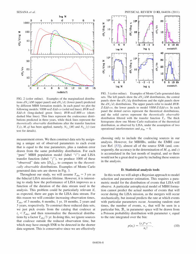
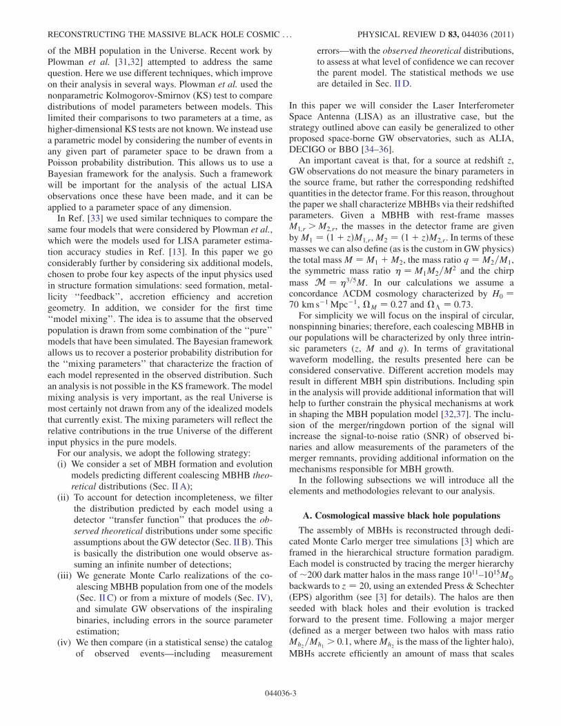
measurement errors. We then construct data sets by assign-ing a unique set of observed parameters to each eventthat is equal to the true parameters, plus a random errordrawn from the same probability distribution. For each‘‘pure’’ MBH population model (label ‘‘i’’) and LISAtransfer function (label ‘‘j’’), we produce 1000 of these‘‘observed’’ data sets fDkgi;j, to compare to the theoreti-

cally observable distributions. Examples of Monte Carlogenerated data sets are shown in Fig. 3.

Throughout our study, we will assume Tobs ¼ 3 yrs asthe fiducial LISA mission lifetime. However, it is interest-ing to study how the performance of LISA improves as afunction of the duration of the data stream used in theanalysis. This problem could be particularly relevant if,as expected, there are gaps in the LISA data stream. Forthis reason we will consider increasing observation times,Tobs, of 3 months, 6 months, 1 yr, 18 months, 2 years and3 years, respectively. To construct these reduced data sets,we just pick events from the catalog that coalesce attc < Tobs, and then renormalize the theoretical distribu-tions by a factor Tobs=3 yr. In doing this, we ignore sourcesthat coalesce outside the reduced observation time, butwhich may have enough SNR to be detected in the shorterdata segment. This is conservative since we are effectively

choosing only to include the coalescing sources in ouranalysis. However, for MBHBs, unlike the EMRI case(see Ref. [53]), almost all of the source SNR (and, con-sequently, the accuracy in the determination ofM, q, and z)is accumulated in the last month of inspiral, and so therewould not be a great deal to gain by including these sourcesin the analysis.

D. Statistical analysis tools

In this work we will adopt a Bayesian approach to modelselection and parameter estimation. This requires a para-metric model for the distribution of events that LISA willobserve. A particular astrophysical model of MBH forma-tion cannot predict the actual number of events that willoccur during the LISA mission, as the mergers will occurstochastically, but instead predicts the rate at which eventswith particular parameters occur. Assuming random starttimes, the number of events, ni, that will be seen in aparticular bin, Bi, in parameter space will be drawn froma Poisson probability distribution with parameter ri equalto the rate integrated over the bin:

pðniÞ ¼ ðriÞnieri

ni!: (10)

FIG. 3 (color online). Examples of Monte Carlo generated datasets. The left panels show the dNi=dM distributions, the centralpanels show the dNi=dq distributions and the right panels showthe dNi=dz distributions. The upper panels refer to model BVR-Z-Edd-co, the lower panels to model VHM-Z-Edd-co. In eachpanel the dotted curves represent the theoretical distributions,and the solid curves represent the theoretically observabledistribution filtered with the transfer function T3. The thickhistograms show one Monte Carlo realization of the theoreticaldistribution, as observed by LISA, under the assumption of twooperational interferometers and thr ¼ 8.

FIG. 2 (color online). Examples of the marginalized distribu-tions dNi=dM (upper panel) and dNi=dz (lower panel) predictedby different MBH formation models. In each panel we plot thefollowing models: VHM-noZ-Edd-co (solid red lines); BVR-noZ-Edd-ch (long-dashed green lines); BVR-noZ-MH-co (short-dashed blue lines). Thin lines represent the coalescence distri-butions predicted in three years, while thick lines represent thetheoretically observable distributions after the transfer functionT3ðz;M; qÞ has been applied, namely, NTi;3

ðMÞ and NTi;3ðzÞ (see

text for details).


044036-8

If we divide the parameter space up into a certain numberof bins, K say, then the information that comes from LISA(the data D) is the number of events in each bin. The

overall likelihood, pðDj ~; XÞ of seeing this data under

the model X with parameters ~ is the product of thePoisson probabilities for each bin

pðDj ~; XÞ ¼ YKi¼1

ðrið ~ÞÞnierið ~Þ

ni!: (11)

The rates that enter this expression are the rates for ob-served events, i.e., the product of the intrinsic rate pre-dicted by the model with the LISA transfer function, asdiscussed in the previous section. It is straightforward totake the limit of this expression as the bin sizes tend to zeroto derive a continuum version of this equation [53].

LISA will not be able to measure the parameters ofeach system perfectly due to instrumental noise. In addi-tion, weak-lensing will introduce errors in the measure-ments of luminosity distance. Since we wish to use redshiftrather than distance as a parameter, further errors will beintroduced from imperfect knowledge of the luminositydistance-redshift relation. The modeling of these errorswas mentioned earlier, and is described in detail inAppendix A. There are two ways in which the errors canbe folded into the statistical analysis. Once LISA observa-tions have been made, we will obtain posterior probabilitydistributions for the source parameters which account forthe error-induced uncertainties. The likelihood will then becomputed by integrating the continuum version of Eq. (11)over the posterior, as described in [53]. The second ap-proach, which we adopt here as it is more appropriate for apriori studies of this type, is to fold the expected errors intothe computation of the observed rates, ri. In practice, wecompute these rates directly from the Monte Carlo realiza-tions described in the preceding section. For each source inthe catalog we can assign fractional rates to every bin inparameter space, computed by integrating the error proba-bility distribution for the source over that particular bin.In other words, we spread each source out into multiplebins, as predicted by the error model described earlier.When generating realizations of the LISA data set, weassign each source to one bin only, according to some‘‘observed parameters’’ (which could represent, for in-stance, the maximum a posteriori parameters of thesource). We take these observed parameters to be equalto the true parameters plus an error drawn from the sameerror distribution.

Given the likelihood described above, Bayes theorem

allows us to assign a posterior probability, pð ~jD;XÞ, to theparameters, ~, of a model, X, given the observed data, D,

and a prior, ð ~Þ, for the parameters ~:

pð ~jD;XÞ¼pðDj ~;XÞð ~ÞZ

; Z¼ZpðDj ~;XÞð ~ÞdN:

(12)

When comparing two models, A and B, that could eachdescribe the data, we can compute the odds ratio (see, forexample, [54])

OAB ¼ ZAPðAÞZBPðBÞ ; (13)

in which PðXÞ denotes the prior probability assigned tomodel X. If OAB 1ðOAB 1Þ, model A (model B)provides a much better description of the data.In this paper, we will consider two types of model

comparison. In Sec. IV, we will consider mixed modelsin which the observed distribution is drawn from a super-position of two or more of the underlying ‘‘pure’’ models.In those cases, the models depend on one or more free‘‘mixing’’ parameters for which we will obtain posteriordistributions using Eq. (12). First, however, in Sec. III, wewill make direct comparisons between the pure models. Inthat case, the models do not have any free parameters. Theodds ratio, (13), then reduces to the product of the like-lihood ratio with the prior ratio

OAB ¼ pðDjAÞPðAÞpðDjBÞPðBÞ : (14)

The models we consider have all been tuned to matchexisting constraints, and so at present we have no goodreason to prefer one model over the others. We thereforeassign equal prior probability to each pure model, PðAÞ ¼PðBÞ ¼ 0:5, and the odds ratio becomes the likelihoodratio. We assign probability pA ¼ pðDjAÞ=ðpðDjAÞ þpðDjBÞÞ to model A, and pB ¼ 1 pA to model B.Once LISA data is available, each model comparison

will yield this single number, pA, which is our confidencethat model A is correct. Since the LISA data is not currentlyavailable, we want to work out how likely it is that we willachieve a certain confidence with LISA. So, we generate1000 realizations of the LISA data stream and look at thedistribution of the likelihood ratio and confidence overthese realizations. We can represent the results of thisanalysis in two alternative ways. These are illustrated inFig. 4, and we will refer to the two panels of this figureextensively in the following. The left panel shows a re-ceiver operator characteristic (ROC) curve. This is a‘‘frequentist’’ way to represent the data. To generate thisplot, we assume that we have specified a threshold on thestatistic, in this case the likelihood ratio, before the data iscollected. If the value of the statistic computed for theobserved data exceeds the threshold then model A ischosen, otherwise model B is chosen. For a given thresh-old, the frequency with which the threshold is exceeded forrealizations of model B defines the false alarm probability(FAP), while the frequency with which the threshold is


044036-9

exceeded for realizations of model A defines the detectionrate. The ROC curve shows detection rate vertically versusFAP horizontally. In the figure, we indicate how, for anFAP of 10%, we can find the detection rate, which in thiscase is 49%. This is the format we used to present ourprevious results in Ref. [33]. While the ROC is a conve-nient way to represent the data, it is incomplete, in that itdoes not tell us by how much we exceed the threshold: theresult is far more convincing if we obtain a likelihood ratio10 times the threshold, than 1.1 times the threshold.

The right panel of Fig. 4 shows an alternative represen-tation of the same data which contains this additionalinformation. It shows the cumulative distribution function(CDF) for the ‘‘confidence’’ we would have in model A,based on our observation, i.e., the probability, pA, weassign to model A in a Bayesian interpretation of the resultsof an observation. The upper curve is the CDF computedover multiple realizations of model A (i.e., the horizontalaxis then shows our confidence in the true model), whilethe lower curve shows the CDF computed from realizationsof model B (i.e., the horizontal axis then shows our con-fidence in the wrong model). The best way to interpret thisplot is to choose a certain confidence level, e.g., p ¼ 0:95(approximately 2). The value on the upper curve is thefrequency with which this confidence level, or better,would be achieved in a LISA observation when that modelwas correct, while the value on the lower curve at 1 p isthe frequency with which we would not be able to rule outmodel A with that confidence, when it was not true.

The CDF plot encodes the same information as the ROCcurve. If we assign a certain FAP, say 10% as before, wedraw a horizontal line at that value and find where itintersects the lower curve. This tells us the confidence levelcorresponding to that FAP, in this case 0.67. The value on

the upper curve at this confidence level is the detection rateat that FAP, and we find that it is 49%, as expected. In thecurrent paper, we will use this second, Bayesian, represen-tation of the results for all the remaining plots, as it encodesall of the information that can be gleaned from theMonte Carlo simulations. The Bayesian approach assignsrelative probabilities to the models, rather than making abinary statement that model A is ‘‘right’’ or model B is‘‘right’’.The models we consider differ not only in the distribu-

tion of events that they predict, but also in the total numberof events. As the latter could be considered a less robustprediction of the models, we can ask whether it carriesmuch weight for model selection. This can be done byintroducing a free parameter into each model, which is anoverall normalizing factor, and then marginalizing over it,i.e., integrating the posterior probability over this parame-ter. We write ri ¼ N~ri, where ~ri is the rate in bin i for amodel that predicts 1 event in total. The probability margi-nalized over N is

~pðDjXÞ ¼YKi¼1

~rniini!

X1n¼1

nNobsen; (15)

where Nobs ¼P

ni is the total number of events observed.The summation in the second term is dependent only onNobs and, as such, is model-independent. It can thus beseen that

~pðDjXÞ / pðDjXÞeNXNNobs

X ; (16)

where NX is the number of events predicted by the un-normalized model X. We can decouple the contributionfrom the total number of events and the distribution ofevent parameters by replacing the likelihood pðDjXÞ by the

0

0.1

0.2

0.3

0.4

0.5

0.6

0.7

0.8

0.9

1

0 0.2 0.4 0.6 0.8 1

Det

. Rat

e

FAP

0.490.49

0

0.1

0.2

0.3

0.4

0.5

0.6

0.7

0.8

0.9

1

0 0.2 0.4 0.6 0.8 1

P(p

1 >

p)

Confidence (p)

0.67

0.49

True modelAlternative model

FIG. 4 (color online). Two alternative ways to represent our ability to distinguish models. The left panel shows an ROC curve, whilethe right panel shows the CDF of the confidence achieved over multiple realizations of the correct (upper curve) and wrong (lowercurve) model. More details are given in the text. The model comparison used for this figure was VHM-noZ-Edd-co to VHM-noZ-Edd-ch, for a three-month LISA observation and the most pessimistic assumption (T2) on the transfer function.


044036-10

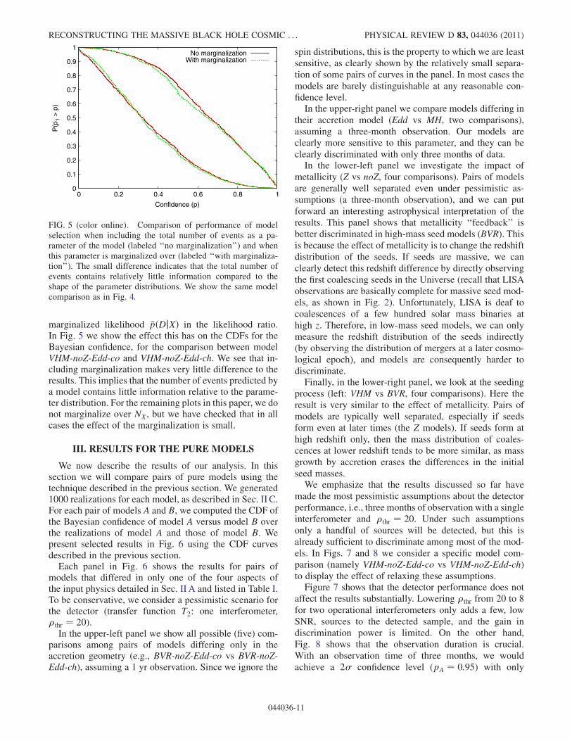
marginalized likelihood ~pðDjXÞ in the likelihood ratio.In Fig. 5 we show the effect this has on the CDFs for theBayesian confidence, for the comparison between modelVHM-noZ-Edd-co and VHM-noZ-Edd-ch. We see that in-cluding marginalization makes very little difference to theresults. This implies that the number of events predicted bya model contains little information relative to the parame-ter distribution. For the remaining plots in this paper, we donot marginalize over NX, but we have checked that in allcases the effect of the marginalization is small.

III. RESULTS FOR THE PURE MODELS

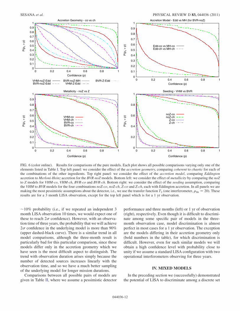
We now describe the results of our analysis. In thissection we will compare pairs of pure models using thetechnique described in the previous section. We generated1000 realizations for each model, as described in Sec. II C.For each pair of models A and B, we computed the CDF ofthe Bayesian confidence of model A versus model B overthe realizations of model A and those of model B. Wepresent selected results in Fig. 6 using the CDF curvesdescribed in the previous section.

Each panel in Fig. 6 shows the results for pairs ofmodels that differed in only one of the four aspects ofthe input physics detailed in Sec. II A and listed in Table I.To be conservative, we consider a pessimistic scenario forthe detector (transfer function T2: one interferometer,thr ¼ 20).

In the upper-left panel we show all possible (five) com-parisons among pairs of models differing only in theaccretion geometry (e.g., BVR-noZ-Edd-co vs BVR-noZ-Edd-ch), assuming a 1 yr observation. Since we ignore the

spin distributions, this is the property to which we are leastsensitive, as clearly shown by the relatively small separa-tion of some pairs of curves in the panel. In most cases themodels are barely distinguishable at any reasonable con-fidence level.In the upper-right panel we compare models differing in

their accretion model (Edd vs MH, two comparisons),assuming a three-month observation. Our models areclearly more sensitive to this parameter, and they can beclearly discriminated with only three months of data.In the lower-left panel we investigate the impact of

metallicity (Z vs noZ, four comparisons). Pairs of modelsare generally well separated even under pessimistic as-sumptions (a three-month observation), and we can putforward an interesting astrophysical interpretation of theresults. This panel shows that metallicity ‘‘feedback’’ isbetter discriminated in high-mass seed models (BVR). Thisis because the effect of metallicity is to change the redshiftdistribution of the seeds. If seeds are massive, we canclearly detect this redshift difference by directly observingthe first coalescing seeds in the Universe (recall that LISAobservations are basically complete for massive seed mod-els, as shown in Fig. 2). Unfortunately, LISA is deaf tocoalescences of a few hundred solar mass binaries athigh z. Therefore, in low-mass seed models, we can onlymeasure the redshift distribution of the seeds indirectly(by observing the distribution of mergers at a later cosmo-logical epoch), and models are consequently harder todiscriminate.Finally, in the lower-right panel, we look at the seeding

process (left: VHM vs BVR, four comparisons). Here theresult is very similar to the effect of metallicity. Pairs ofmodels are typically well separated, especially if seedsform even at later times (the Z models). If seeds form athigh redshift only, then the mass distribution of coales-cences at lower redshift tends to be more similar, as massgrowth by accretion erases the differences in the initialseed masses.We emphasize that the results discussed so far have

made the most pessimistic assumptions about the detectorperformance, i.e., three months of observation with a singleinterferometer and thr ¼ 20. Under such assumptionsonly a handful of sources will be detected, but this isalready sufficient to discriminate among most of the mod-els. In Figs. 7 and 8 we consider a specific model com-parison (namely VHM-noZ-Edd-co vs VHM-noZ-Edd-ch)to display the effect of relaxing these assumptions.Figure 7 shows that the detector performance does not

affect the results substantially. Lowering thr from 20 to 8for two operational interferometers only adds a few, lowSNR, sources to the detected sample, and the gain indiscrimination power is limited. On the other hand,Fig. 8 shows that the observation duration is crucial.With an observation time of three months, we wouldachieve a 2 confidence level (pA ¼ 0:95) with only

0

0.1

0.2

0.3

0.4

0.5

0.6

0.7

0.8

0.9

1

0 0.2 0.4 0.6 0.8 1

P(p

1 >

p)

Confidence (p)

No marginalizationWith marginalization

FIG. 5 (color online). Comparison of performance of modelselection when including the total number of events as a pa-rameter of the model (labeled ‘‘no marginalization’’) and whenthis parameter is marginalized over (labeled ‘‘with marginaliza-tion’’). The small difference indicates that the total number ofevents contains relatively little information compared to theshape of the parameter distributions. We show the same modelcomparison as in Fig. 4.


044036-11

10% probability (i.e., if we repeated an independent 3month LISA observation 10 times, we would expect one ofthese to reach 2 confidence). However, with an observa-tion time of three years, the probability that wewill achieve2 confidence in the underlying model is more than 90%(upper dashed-black curve). There is a similar trend in allmodel comparisons, although the three-month result isparticularly bad for this particular comparison, since thesemodels differ only in the accretion geometry which wehave seen is the most difficult aspect to distinguish. Thetrend with observation duration arises simply because thenumber of detected sources increases linearly with theobservation time, and so we have a much better samplingof the underlying model for longer mission durations.

Comparisons between all possible pairs of models aregiven in Table II, where we assume a pessimistic detector

performance and three months (left) or 1 yr of observation(right), respectively. Even though it is difficult to discrimi-nate among some specific pair of models in the three-month observation case, model discrimination is almostperfect in most cases for a 1 yr observation. The exceptionare the models differing in their accretion geometry only(bold numbers in the table), for which discrimination isdifficult. However, even for such similar models we willobtain a high confidence level with probability close tounity if we assume a standard LISA configuration with twooperational interferometers observing for three years.

IV. MIXED MODELS

In the preceding section we (successfully) demonstratedthe potential of LISA to discriminate among a discrete set

0

0.1

0.2

0.3

0.4

0.5

0.6

0.7

0.8

0.9

1

0 0.2 0.4 0.6 0.8 1

P(p

1 >

p)

Confidence (p)

Accretion Geometry - co vs ch

VHM-noZ-EddBVR-noZ-Edd

BVR-noZ-MHVHM-Z-Edd

BVR-Z-Edd 0

0.1

0.2

0.3

0.4

0.5

0.6

0.7

0.8

0.9

1

0 0.2 0.4 0.6 0.8 1

P(p

1 >

p)

Confidence (p)

Accretion Model - Edd vs MH (for BVR-noZ)

Edd-co vs MH-coEdd-ch vs MH-ch

0

0.1

0.2

0.3

0.4

0.5

0.6

0.7

0.8

0.9

1

0 0.2 0.4 0.6 0.8 1

P(p

1 >

p)

Confidence (p)

Metallicity - noZ vs Z

VHM-coVHM-chBVR-coBVR-ch

0

0.2

0.4

0.6

0.8

1

0 0.2 0.4 0.6 0.8 1

P(p

1 >

p)

Confidence (p)

Seeding - VHM vs BVR

noZ-conoZ-ch

Z-coZ-ch

FIG. 6 (color online). Results for comparisons of the pure models. Each plot shows all possible comparisons varying only one of theelements listed in Table I. Top left panel: we consider the effect of the accretion geometry, comparing coherent to chaotic for each ofthe combinations of the other ingredients. Top right panel: we consider the effect of the accretion model, comparing Eddingtonaccretion toMerloni-Heinz accretion for the BVR-noZ models. Bottom left: we consider the effect of metallicity by comparing the noZto Z models for VHM-co, VHM-ch, BVR-co and BVR-ch. Bottom right: we consider the effect of the seeding assumption, comparingthe VHM to BVR models for the four combinations noZ-co, noZ-ch, Z-co and Z-ch, each with Eddington accretion. In all panels we aremaking the most pessimistic assumptions about the detector, i.e., we use the transfer function T2 (one interferometer, thr ¼ 20). Theseresults are for a 3 month LISA observation, except for the top left panel which is for a 1 yr observation.


044036-12

0

0.1

0.2

0.3

0.4

0.5

0.6

0.7

0.8

0.9

1

0 0.2 0.4 0.6 0.8 1

P(p

1 >

p)

Confidence (p)

one interferometer, SNR=20one interferometer, SNR=8

two interferometers, SNR=20two interferometers, SNR=8

FIG. 7 (color online). Effect of the transfer function on thepure model selection results. We compare VHM-noZ-Edd-co andVHM-noZ-Edd-ch, assuming a fixed LISA mission duration of 3months.

0

0.1

0.2

0.3

0.4

0.5

0.6

0.7

0.8

0.9

1

0 0.2 0.4 0.6 0.8 1

P(p

1 >

p)

Confidence (p)

3 month6 month

1 year18 month

2 year3 year

FIG. 8 (color online). Effect of the LISA observation durationon the pure model selection results. We compare VHM-noZ-Edd-co and VHM-noZ-Edd-ch, under the most pessimistic choice (T2)for the transfer function.

TABLE II. Summary of all possible comparisons of the pure models. The table on the left (right) assumes a LISA observation timeof three months (one-year), respectively. Models are labeled by an integer i, as listed in Table I. We take a fixed confidence level ofp ¼ 0:95. The numbers in the upper-right half of each table show the fraction of realizations in which the row model will be chosen atmore than this confidence level when the row model is true (in the Bayesian figures, this would be the point where a vertical line atx ¼ p intersects the upper curve). The numbers in the lower-left half of each table show the fraction of realizations in which the rowmodel cannot be ruled out at that confidence level when the column model is true (in the Bayesian figures, this would be the pointwhere a vertical line at x ¼ 1 p intersects the lower curve). These results are for the pessimistic transfer function (T2).

Three-month observation

1 2 3 4 5 6 7 8 9 10

1 0.10 0.72 0.68 0.86 0.88 0.19 0.17 0.91 0.92

2 0.93 0.75 0.69 0.91 0.91 0.17 0.22 0.93 0.93

3 0.42 0.32 0.24 0.45 0.42 0.72 0.69 0.88 0.89

4 0.65 0.63 0.83 0.77 0.76 0.48 0.49 0.80 0.81

5 0.13 0.08 0.58 0.19 0.03 0.93 0.92 0.98 0.99

6 0.12 0.07 0.58 0.21 0.97 0.94 0.92 0.98 0.98

7 0.57 0.57 0.16 0.20 0.05 0.04 0.01 0.93 0.94

8 0.58 0.51 0.16 0.19 0.07 0.07 0.98 0.94 0.95

9 0.16 0.12 0.23 0.31 0.03 0.04 0.17 0.15 0.01

10 0.09 0.07 0.15 0.18 0.02 0.03 0.14 0.13 0.95

One-year observation

1 2 3 4 5 6 7 8 9 10

1 0:49 0.99 0.99 1.00 1.00 0.91 0.88 1.00 1.00

2 0:50 0.99 0.99 1.00 1.00 0.92 0.93 1.00 1.00

3 0.00 0.00 0:83 0.97 0.97 1.00 1.00 1.00 1.00

4 0.02 0.02 0:19 0.99 0.99 0.99 0.99 0.99 0.99

5 0.00 0.00 0.03 0.00 0:07 1.00 1.00 1.00 1.00

6 0.00 0.00 0.03 0.00 0:93 1.00 1.00 1.00 1.00

7 0.07 0.06 0.00 0.00 0.00 0.00 0:16 1.00 1.00

8 0.09 0.05 0.00 0.00 0.00 0.00 0:85 1.00 1.00

9 0.00 0.00 0.00 0.01 0.00 0.00 0.00 0.00 0:3110 0.00 0.00 0.00 0.00 0.00 0.00 0.00 0.00 0:61


044036-13

of ‘‘pure’’ models given a priori. However, the true MBHpopulation in the Universe will probably result from amixing of the physical processes described in Sec. II A,or even from a completely unexplored physical mecha-nism. It is therefore important to test whether we will beable to extract useful information when the distribution ofobserved events comes from a mixture of the differentmodels, as an approximation to possible unknowns. Forthis case study, we will concentrate on the details of theseeding mechanism (mass function and redshift distribu-tion), deferring the more complicated details related toaccretion to a future study. Recall in this context thataccretion will leave a trace in the spin distribution ofMBHs, but our simplified analysis neglects the MBH spinsby construction.

We tested two mixing procedures: (i) we generatedartificially mixed models that were a linear combinationof the pure model distributions presented in Sec. II A;(ii) we constructed two consistently mixed models, inwhich seeds were generated according to a mixing of twoprescriptions, and their evolution was followed self-consistently in the halo merger tree realizations. The goalhere is to assess whether artificial models can reproducethe salient features of the consistently mixed models, andto estimate the amount of mixing necessary to ‘‘best fit’’the consistently mixed models. This procedure mimics theanalysis of a ‘‘real’’ LISA datastream, for which the datais unlikely to match exactly any one of the pure modelpredictions.

In this section we describe details of the artificially andconsistently mixed models. In Sec. V that follows we willpresent the results of the ‘‘reconstruction experiment’’.

Artificial mixing simply consists in drawing coales-cences from a linear combination of the theoretical coales-cence distributions predicted by the pure models. Here, forconcreteness, we fix the accretion to be Eddington-limitedand coherent, and we mix different seeding recipes. Wetherefore consider models VHM-noZ-Edd-co, VHM-Z-Edd-co, BVR-noZ-Edd-co, and BVR-Z-Edd-co (i ¼ 1, 3,5 and 7, respectively, in the notation of Table I).

Each model i is characterized by a mean number ofpredicted coalescences Ni and a probability distribution

for the parameters of the coalescing binaries piðM;q; zÞ.The predicted event distribution N i ¼ d3Ni=dzdMdq(see Sec. II A) can therefore be factorized as

N i ¼ Ni piðM;q; zÞ: (17)

The mixing is described by four parameters fi (i ¼ 1, 3, 5,7) which determine the fraction of model i included inthe mixed distribution. These fractions are constrained toadd up to 1.

A. Artificial mixing

We tried two different mixing prescriptions. In the firstcase we ignored the number of coalescences predicted byeach specific model, by mixing the respective piðM;q; zÞdistributions (p mixing) and normalizing the mixed distri-bution to some arbitrary number:

N p ¼ Nmff1p1 þ f3p3 þ f5p5 þ f7p7g; (18)

where Nm was fixed to 200 coalescences in three years. Inthe second case we considered the number of predictedevents to be an intrinsic property of each individual model,and we simply mixed the NiðM;q; zÞ distributions (Nmixing) in the same way:

N N ¼ f1N 1 þ f3N 3 þ f5N 5 þ f7N 7: (19)

The total number of coalescences is now automaticallydetermined by the values of the mixing parameters. Inpractice, in order to enforce the constraint that the fractionsadd up to 1, we actually use a ‘‘nested’’ prescription basedon three parameters , and , which are allowed to takeany value in the range [0, 1]. We then set

N N ¼ N 1 þ ð1 ÞfN 3

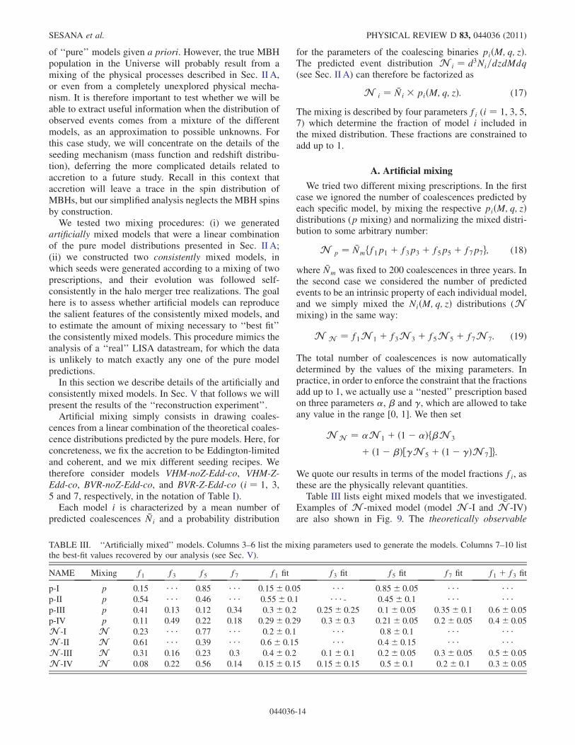
þ ð1 Þ½N 5 þ ð1 ÞN 7g:We quote our results in terms of the model fractions fi, asthese are the physically relevant quantities.Table III lists eight mixed models that we investigated.

Examples of N -mixed model (model N -I and N -IV)are also shown in Fig. 9. The theoretically observable

TABLE III. ‘‘Artificially mixed’’ models. Columns 3–6 list the mixing parameters used to generate the models. Columns 7–10 listthe best-fit values recovered by our analysis (see Sec. V).

NAME Mixing f1 f3 f5 f7 f1 fit f3 fit f5 fit f7 fit f1 þ f3 fit

p-I p 0.15 0.85 0:15 0:05 0:85 0:05 p-II p 0.54 0.46 0:55 0:1 - 0:45 0:1 p-III p 0.41 0.13 0.12 0.34 0:3 0:2 0:25 0:25 0:1 0:05 0:35 0:1 0:6 0:05p-IV p 0.11 0.49 0.22 0.18 0:29 0:29 0:3 0:3 0:21 0:05 0:2 0:05 0:4 0:05N -I N 0.23 0.77 0:2 0:1 0:8 0:1 N -II N 0.61 0.39 0:6 0:15 0:4 0:15 N -III N 0.31 0.16 0.23 0.3 0:4 0:2 0:1 0:1 0:2 0:05 0:3 0:05 0:5 0:05N -IV N 0.08 0.22 0.56 0.14 0:15 0:15 0:15 0:15 0:5 0:1 0:2 0:1 0:3 0:05


044036-14

distributions are generated in the same way as for the puremodels, by multiplying the N distributions by the appro-priate transfer function. Observed data sets Dk are thengenerated from the mixed distribution as outlined inSec. II C. Given a data set Dk, the idea is to parametrizethe distribution as a mixture of the available ‘‘pure’’ dis-tributions according to Eqs. (18) or (19), and obtain aposterior distribution for the mixing parameters given theobserved data. These posterior distributions allow us toassess which models were mixed, and at what mixing level.To make the test ‘‘realistic’’, the theoretical mixing andthe simulated LISA observations were performed byA. Sesana. The observed data sets Dk were then analyzedblindly by J. Gair, who did not know which models weremixed nor the amount of mixing.

B. Consistent mixing

We used the consistently mixed models (hybrid models,henceforth labeled ‘‘HY’’) described in Ref. [24].The seeding process was a mixture of the VHM-Z andBVR-Z mechanisms, and the MBH mass growth assumed

Eddington-limited, coherent accretion. We considered twomodels with fixed POPIII seeding, but different quasistarseeding efficiencies. The quasistar seeding efficiency isrelated to the maximum halo spin parameter, , thatallows efficient transfer of gas to the center to form aquasistar (see Ref. [24] for details). We test an inefficientquasistar seeding model ( ¼ 0:01, HY-I) and an effi-cient quasistar seeding model ( ¼ 0:02, HY-II) that pre-dict MBH population observables (local mass function,quasar luminosity function, and so on) bracketing thecurrent range of allowed values.To check the effectiveness of our analysis tools in ex-

tracting information about the parent MBH population, wetry to recover the hybrid model distributions as a mixing ofthe VHM-Z and BVR-Z ‘‘pure’’ models, of the form givenby either Eq. (18) or (19). The procedure is the same asdetailed in the previous section.Let us stress again that the MBH evolution through

cosmic history is followed self-consistently in the hybridmodels. This means that the predicted theoretical distribu-tion is not, in general, described as a simple mixing of theform given by Eqs. (18) or (19). This is a crucial point: thesuccess of this experiment will tell us that we can extractvaluable information on complex MBH formation scenar-ios by mixing a set of ‘‘pure’’ models based on simplerecipes.

V. RESULTS FOR THE MIXED MODELS

In the context of mixed models, we are no longer com-paring two preassigned models A and B as descriptionsof the observational data. We deal instead with a single,continuous parameter space of models, where the parame-ters are the mixing fractions of some subset of ‘‘pure’’models. For example, if we mix models 1 and 3, we have aone-dimensional parameter space given by the contributionof model 1 (f1) to the total population (the contribution ofmodel 3 is fixed by the constraint f1 þ f3 ¼ 1). Given aparticular observation, we can then compute the posteriorprobability distribution function (PDF) given by Bayestheorem, Eq. (12), for the mixing fractions. The computa-tion of the posterior can be done either over a grid of pointsin the parameter space, or by exploring the parameter spaceby means of Markov Chain Monte Carlo simulations(which become much more practical as the dimension ofthe parameter space increases).For each mixed model, 100 different realizations of the

LISA data were generated and a posterior probabilitydistribution for the mixing fractions was obtained foreach one. The width of the posterior in a single realizationreflects how well that particular data set can constrain themixing fractions. The location of the peak of the posteriorwill change from realization to realization, but we wouldexpect the width to remain approximately the same. Wealso expect that the distribution of the location of the peakof the posterior over many realizations should resemble the

FIG. 9 (color online). Examples of mixed models. In the upperpanels we show marginalized dNi=dM (left) and dNi=dz (right)distributions for the model N -I (thick solid black lines), inwhich we mix models VHM-noZ-Edd-co (thin solid red line) andBVR-noZ-Edd-co (thin long-dashed green line). The relativecontribution of the models is given by Eq. (19) with f1 ¼0:23, f3 ¼ 0:77 (cf. Table II). In the lower panels we show thesame distributions for the model N -IV (thick solid black lines)in which we mix four ‘‘pure’’ models. The thin lines representthe relative contribution of the individual models VHM-noZ-Edd-co (solid red), VHM-Z-Edd-co (short-dashed blue), BVR-noZ-Edd-co (long-dashed green), and BVR-Z-Edd-co (dot-dashed magenta). The relative contribution of the models isgiven again by Eq. (19) with f1 ¼ 0:08, f3 ¼ 0:22, f5 ¼ 0:56and f7 ¼ 0:14 (cf. Table II).


044036-15

posterior for the mixing fractions computed in any singlerealization.

We considered a total of eight different mixed models, aslisted in Table III, mixing either just VHM-noZ-Edd-co andBVR-noZ-Edd-co or these two models plus VHM-Z-Edd-coand BVR-Z-Edd-co. For each case, we assumed that wewere using three years of LISA data, but made pessimisticassumptions (T2) for the transfer function. While this latterassumption is slightly conservative, we checked that therewas not much difference in performance when using themost optimistic assumptions (i.e., the transfer function T3).

The posterior distributions of the mixing fraction foundin one particular realization each of modelsN -I andN -IIare shown in the left panel of Fig. 10. The PDFs peakaround f1 ¼ 0:2 0:05 for model N -I and f1 ¼ 0:550:1 for model N -II, which is consistent with the injectedfractions listed in Table III.

As mentioned above, we expect the peak and width ofthe posterior PDF to fluctuate from realization to realiza-tion. To assess the statistical robustness of this result wetherefore repeat the experiment. In the right panel ofFig. 10, we plot the distribution of the location of thepeak of the posterior PDF found in each of 100 realizations

of the models. As we expect, the widths of these distribu-tions are very similar to the PDFs found in each of theindividual realizations. The distribution peaks around f1 ¼0:2 0:05 for modelN -I and around f1 ¼ 0:55 0:1 formodel N -II, in agreement with the true injected fractionslisted in Table III. This experiment shows that most of thetime we can correctly infer the relative contribution of thetwo models, but there is still the possibility to draw erro-neous conclusions from a single observation. For example,in two realizations of model N -II we would prefer analmost pure VHM model, while the underlying distributionis in fact 45% BVR. However, in these cases the posteriorPDF is also very wide, which would be an indicator that thedata set was not placing particularly good constraints onthe model in that specific case.Figure 11 shows the results for the more complex case of

model N -III, where all four of the pure models weremixed and the mixing parameter space is three-dimensional. Again, both the posterior PDFs given by aspecific realization (left panel) and the distribution of thepeak values of the posterior PDFs in a sample of 100realizations return mixing fractions which are consistentwith the injected values (see Table III). However, in this

0

1

2

3

4

5

6

0 0.2 0.4 0.6 0.8 1

f1

N-IN-II

0

1

2

3

4

5

6

0 0.2 0.4 0.6 0.8 1

f1

N-IN-II

FIG. 10 (color online). Summary of the model mixing results for models N -I and N -II. In both panels, the horizontal axis showsthe mixing fraction for model VHM-noZ-Edd-co. The left panel shows the posterior probability distribution function for this mixingfraction as found in one particular realization of each model. The right panel shows how the peak of the posterior was distributed over100 different realizations of each of the two models. The vertical lines show the true values of the mixing fraction.

0

1

2

3

4

5

0 0.1 0.2 0.3 0.4 0.5 0.6 0.7 0.8 0.9

Fraction

VHMBVR

VHMZBVRZ

0

1

2

3

4

5

0 0.1 0.2 0.3 0.4 0.5 0.6 0.7 0.8 0.9 1

Fraction

BVRBVRZ

VHM+VHMZ

0

1

2

3

4

5

6

7

8

0 0.2 0.4 0.6 0.8 1

Fraction

VHMBVR

VHMZBVRZ

VHM + VHMZ

FIG. 11 (color online). Summary of model mixing results for model N -III. We show the mixing fraction of the given model on thehorizontal axis. The left panel shows the posterior probability distribution of the mixing fraction for each of the four models, VHM,BVR, VHM-Z and BVR-Z, found when analyzing a single realization of modelN -III. The central panel shows the same thing, but nowconsidering the fractions of BVR, BVR-Z and the sum VHM+VHM-Z in the mixed model. The right panel shows the distribution of thepeak of the posterior pdf found over 100 different realizations of the N -III model.


044036-16

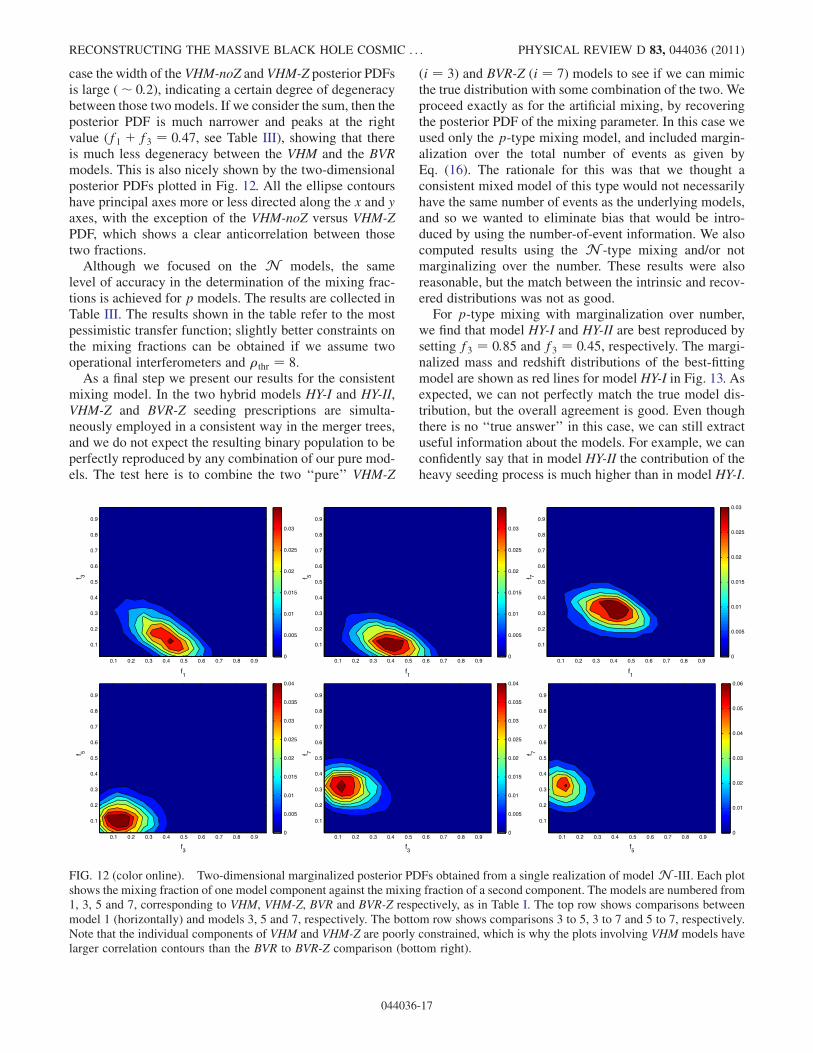
case the width of the VHM-noZ and VHM-Z posterior PDFsis large ( 0:2), indicating a certain degree of degeneracybetween those two models. If we consider the sum, then theposterior PDF is much narrower and peaks at the rightvalue (f1 þ f3 ¼ 0:47, see Table III), showing that thereis much less degeneracy between the VHM and the BVRmodels. This is also nicely shown by the two-dimensionalposterior PDFs plotted in Fig. 12. All the ellipse contourshave principal axes more or less directed along the x and yaxes, with the exception of the VHM-noZ versus VHM-ZPDF, which shows a clear anticorrelation between thosetwo fractions.

Although we focused on the N models, the samelevel of accuracy in the determination of the mixing frac-tions is achieved for p models. The results are collected inTable III. The results shown in the table refer to the mostpessimistic transfer function; slightly better constraints onthe mixing fractions can be obtained if we assume twooperational interferometers and thr ¼ 8.

As a final step we present our results for the consistentmixing model. In the two hybrid models HY-I and HY-II,VHM-Z and BVR-Z seeding prescriptions are simulta-neously employed in a consistent way in the merger trees,and we do not expect the resulting binary population to beperfectly reproduced by any combination of our pure mod-els. The test here is to combine the two ‘‘pure’’ VHM-Z

(i ¼ 3) and BVR-Z (i ¼ 7) models to see if we can mimicthe true distribution with some combination of the two. Weproceed exactly as for the artificial mixing, by recoveringthe posterior PDF of the mixing parameter. In this case weused only the p-type mixing model, and included margin-alization over the total number of events as given byEq. (16). The rationale for this was that we thought aconsistent mixed model of this type would not necessarilyhave the same number of events as the underlying models,and so we wanted to eliminate bias that would be intro-duced by using the number-of-event information. We alsocomputed results using the N -type mixing and/or notmarginalizing over the number. These results were alsoreasonable, but the match between the intrinsic and recov-ered distributions was not as good.For p-type mixing with marginalization over number,

we find that model HY-I and HY-II are best reproduced bysetting f3 ¼ 0:85 and f3 ¼ 0:45, respectively. The margi-nalized mass and redshift distributions of the best-fittingmodel are shown as red lines for model HY-I in Fig. 13. Asexpected, we can not perfectly match the true model dis-tribution, but the overall agreement is good. Even thoughthere is no ‘‘true answer’’ in this case, we can still extractuseful information about the models. For example, we canconfidently say that in model HY-II the contribution of theheavy seeding process is much higher than in model HY-I.

f1

f 3

0.1 0.2 0.3 0.4 0.5 0.6 0.7 0.8 0.9

0.1

0.2

0.3

0.4

0.5

0.6

0.7

0.8

0.9

0

0.005

0.01

0.015

0.02

0.025

0.03

f1

f 5

0.1 0.2 0.3 0.4 0.5 0.6 0.7 0.8 0.9

0.1

0.2

0.3

0.4

0.5

0.6

0.7

0.8

0.9

0

0.005

0.01

0.015

0.02

0.025

0.03

f1

f 7

0.1 0.2 0.3 0.4 0.5 0.6 0.7 0.8 0.9

0.1

0.2

0.3

0.4

0.5

0.6

0.7

0.8

0.9

0

0.005

0.01

0.015

0.02

0.025

0.03

f3

f 5

0.1 0.2 0.3 0.4 0.5 0.6 0.7 0.8 0.9

0.1

0.2

0.3

0.4

0.5

0.6

0.7

0.8

0.9

0

0.005

0.01

0.015

0.02

0.025

0.03

0.035

0.04

f3

f 7

0.1 0.2 0.3 0.4 0.5 0.6 0.7 0.8 0.9

0.1

0.2

0.3

0.4

0.5

0.6

0.7

0.8

0.9

0

0.005

0.01

0.015

0.02

0.025

0.03

0.035

0.04

f5

f 7

0.1 0.2 0.3 0.4 0.5 0.6 0.7 0.8 0.9

0.1

0.2

0.3

0.4

0.5

0.6

0.7

0.8

0.9

0

0.01

0.02

0.03

0.04

0.05

0.06

FIG. 12 (color online). Two-dimensional marginalized posterior PDFs obtained from a single realization of model N -III. Each plotshows the mixing fraction of one model component against the mixing fraction of a second component. The models are numbered from1, 3, 5 and 7, corresponding to VHM, VHM-Z, BVR and BVR-Z respectively, as in Table I. The top row shows comparisons betweenmodel 1 (horizontally) and models 3, 5 and 7, respectively. The bottom row shows comparisons 3 to 5, 3 to 7 and 5 to 7, respectively.Note that the individual components of VHM and VHM-Z are poorly constrained, which is why the plots involving VHM models havelarger correlation contours than the BVR to BVR-Z comparison (bottom right).


044036-17

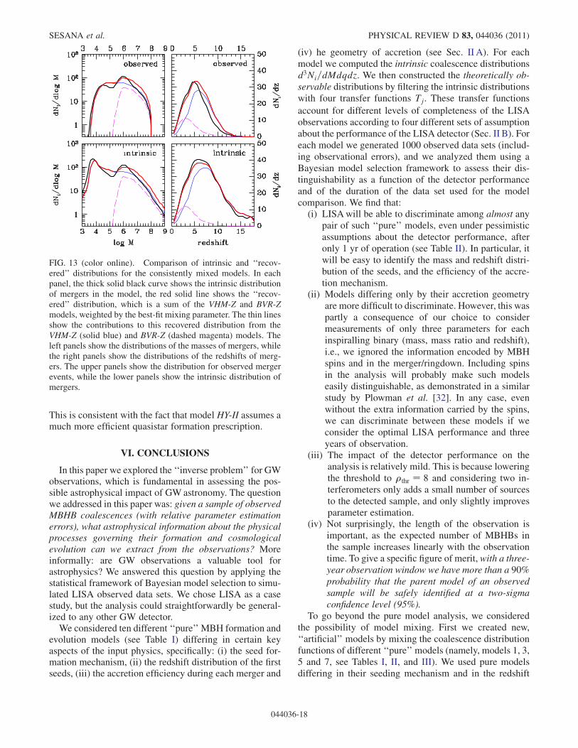
This is consistent with the fact that model HY-II assumes amuch more efficient quasistar formation prescription.

VI. CONCLUSIONS

In this paper we explored the ‘‘inverse problem’’ for GWobservations, which is fundamental in assessing the pos-sible astrophysical impact of GWastronomy. The questionwe addressed in this paper was: given a sample of observedMBHB coalescences (with relative parameter estimationerrors), what astrophysical information about the physicalprocesses governing their formation and cosmologicalevolution can we extract from the observations? Moreinformally: are GW observations a valuable tool forastrophysics? We answered this question by applying thestatistical framework of Bayesian model selection to simu-lated LISA observed data sets. We chose LISA as a casestudy, but the analysis could straightforwardly be general-ized to any other GW detector.

We considered ten different ‘‘pure’’ MBH formation andevolution models (see Table I) differing in certain keyaspects of the input physics, specifically: (i) the seed for-mation mechanism, (ii) the redshift distribution of the firstseeds, (iii) the accretion efficiency during each merger and

(iv) he geometry of accretion (see Sec. II A). For eachmodel we computed the intrinsic coalescence distributionsd3Ni=dMdqdz. We then constructed the theoretically ob-servable distributions by filtering the intrinsic distributionswith four transfer functions Tj. These transfer functions

account for different levels of completeness of the LISAobservations according to four different sets of assumptionabout the performance of the LISA detector (Sec. II B). Foreach model we generated 1000 observed data sets (includ-ing observational errors), and we analyzed them using aBayesian model selection framework to assess their dis-tinguishability as a function of the detector performanceand of the duration of the data set used for the modelcomparison. We find that:(i) LISAwill be able to discriminate among almost any

pair of such ‘‘pure’’ models, even under pessimisticassumptions about the detector performance, afteronly 1 yr of operation (see Table II). In particular, itwill be easy to identify the mass and redshift distri-bution of the seeds, and the efficiency of the accre-tion mechanism.

(ii) Models differing only by their accretion geometryare more difficult to discriminate. However, this waspartly a consequence of our choice to considermeasurements of only three parameters for eachinspiralling binary (mass, mass ratio and redshift),i.e., we ignored the information encoded by MBHspins and in the merger/ringdown. Including spinsin the analysis will probably make such modelseasily distinguishable, as demonstrated in a similarstudy by Plowman et al. [32]. In any case, evenwithout the extra information carried by the spins,we can discriminate between these models if weconsider the optimal LISA performance and threeyears of observation.

(iii) The impact of the detector performance on theanalysis is relatively mild. This is because loweringthe threshold to thr ¼ 8 and considering two in-terferometers only adds a small number of sourcesto the detected sample, and only slightly improvesparameter estimation.

(iv) Not surprisingly, the length of the observation isimportant, as the expected number of MBHBs inthe sample increases linearly with the observationtime. To give a specific figure of merit, with a three-year observation window we have more than a 90%probability that the parent model of an observedsample will be safely identified at a two-sigmaconfidence level (95%).

To go beyond the pure model analysis, we consideredthe possibility of model mixing. First we created new,‘‘artificial’’ models by mixing the coalescence distributionfunctions of different ‘‘pure’’ models (namely, models 1, 3,5 and 7, see Tables I, II, and III). We used pure modelsdiffering in their seeding mechanism and in the redshift

FIG. 13 (color online). Comparison of intrinsic and ‘‘recov-ered’’ distributions for the consistently mixed models. In eachpanel, the thick solid black curve shows the intrinsic distributionof mergers in the model, the red solid line shows the ‘‘recov-ered’’ distribution, which is a sum of the VHM-Z and BVR-Zmodels, weighted by the best-fit mixing parameter. The thin linesshow the contributions to this recovered distribution from theVHM-Z (solid blue) and BVR-Z (dashed magenta) models. Theleft panels show the distributions of the masses of mergers, whilethe right panels show the distributions of the redshifts of merg-ers. The upper panels show the distribution for observed mergerevents, while the lower panels show the intrinsic distribution ofmergers.


044036-18

distribution of the seeds (different metallicity ‘‘feed-back’’). The new models are characterized by the fractionsfi of the ‘‘pure’’ models used in the mixing, with theconstraint

Pifi ¼ 1. Then we considered two hybrid

models, where halos were simultaneously seeded accord-ing to the VHM-Z (i ¼ 3) and the BVR-Z (i ¼ 7) prescrip-tion, and the evolution of the seeds was self-consistentlyfollowed in the halo hierarchy. We produced severalLISA observed data sets for both the artificial and thehybrid models. We then tried to recover the combinationof ‘‘pure’’ models that best reproduces each mixedmodel by maximizing over the posterior probabilitydistribution function of the likelihood (Sec. V). We findthat:

(i) When the ‘‘pure’’ models used in the mixing differonly in their seeding prescription (VHM vs BVR), sothat we have only a single mixing parameter (sinceP

ifi ¼ 1), we can correctly infer this mixing pa-rameter with an accuracy of about 10%.When we mix four different models we can still inferthe mixing fractions with the same accuracy, butthere is a certain degree of degeneracy between thetwo VHM models (i ¼ 1 and i ¼ 5); i.e., the effectof metallicity ‘‘feedback’’, as the detectableMBH population does not differ much between thesetwo models. However, the fraction f1 þ f5 is verywell constrained, and we can clearly distinguish therelative contribution from the different seedingmechanisms.

(ii) Finally, we can also get a fairly good match to thehybrid models by combining ‘‘pure’’ models. Thisis probably the most important result of our analy-sis. The formation and merger history of MBHs is acomplex process, involving several physical ingre-dients which are poorly understood, and it is diffi-cult to imagine that we will have a comprehensivetheoretical understanding of the underlying physicsbefore LISA flies. However, we will certainly beable to construct a set of models based on simplephysical prescriptions that can be tested against theobservations. Our experiment with the hybrid mod-els demonstrates that we can extract valuable infor-mation about more complex MBH formationscenarios by mixing a set of ‘‘pure’’ models basedon simple recipes.

The use of a Bayesian framework is crucial for themodel mixing results, since it allows us to recover aposterior probability distribution for the ‘‘mixing parame-ters’’ that characterizes the fraction of each model contrib-uting to the observed data set. In this respect, our analysisgoes considerably beyond the work recently presented inRef. [32], where only pure models were considered andthe statistical analysis was based on two-dimensionalKolmogorov-Smirnov tests performed on the distributionsof pairs of measured parameters.

Despite this improvement, the building blocks of thepresent work can be improved in many ways. The set ofdistinct ‘‘pure’’ models can not be representative of all thephysical complexity of the problem. A more powerfulapproach to MBH population modeling would be to de-scribe the relevant physics using a set of continuous pa-rameters representing the critical features of the models(seed mass function, accretion efficiency and so on), andthen attempt to measure those parameters by performinga similar Bayesian analysis. We have also adopted severalsimplifying assumptions about the GW observations,which can be refined by developing a more realistic modelfor the GW signal, including spins, higher harmonics,merger and ringdown. We can then attempt a more sophis-ticated analysis and explore the posterior probabilitydistribution function in a larger and more complex parame-ter space, to maximize the recovered information. All theseissues should be explored in the future.Besides the scientific impact of a GW detection in and

by itself, the ambitious goal of doing GW astronomyrequires that we maximize the astrophysical informationthat will be extracted from such detections. In this respect,addressing the ‘‘inverse problem’’ in GW astronomy isextremely important. In this paper we have made a first,small step in this direction. We hope that our work willencourage relativists and GW astronomers to consider ingreater depth the astrophysical impact of GW detections.At the same time, we hope to convince ‘‘ordinary’’ astron-omers that GWs can be an important tool, not only for testsof general relativity and as a laboratory for fundamentalphysics, but also in astrophysics.

ACKNOWLEDGMENTS

J. G’s work is supported by the Royal Society. EB’sresearch was supported by NSF grant PHY-0900735.M.V. was supported by NASA ATP GrantNNX07AH22G and a Rackham faculty grant.

APPENDIX A: ERROR MODELING

We describe here how measurement errors are includedin the analysis. Errors arise due to instrumental noise inthe LISA detector, and from the transformation betweendifferent coordinates. The error propagation expressionsdescribed below are probably not new, and the end result isexpected, but we include the derivation here for complete-ness and to clarify the underlying assumptions.LISA observations will determine the luminosity dis-

tance to a given source, but we want to characterize thesource by the redshift instead. The conversion can be doneusing the concordance cosmology at the time LISA flies,but this introduces additional errors, since the cosmologi-cal parameters will be known imperfectly. Suppose wewant parameters ~x which are given by the measured pa-

rameters, ~y, and a transformation ~xð ~y; ~Þ that depends on


044036-19

some imperfectly known parameters, ~. Suppose further

that the probability distribution for ~ is Lð ~Þ and that for ~yis Yð ~yÞ. The probability distribution for ~x is then

Xð ~xÞ ¼Z

Lð ~ÞYð ~yð ~x; ~ÞÞJð ~x;Þdn; (A1)

in which Jð ~x;Þ is the Jacobian for the transformation

between ~y and ~x and n is the dimensionality of the ~parameter space. We now make two simplifying assump-

tions: (i) the distributions of the errors in ~y and ~ aremultivariate Gaussians with inverse variance-covariancematrices y and , respectively; (ii) the errors are small,so that the distributions are peaked near the true values of~y0 and 0. This latter assumption means that we can use alinear approximation in the interesting region of the dis-tributions

yið ~x; ~Þ yið ~x0;0Þ þ @yi@xj

ðxj x0jÞ þ @yi@j

ðj 0jÞ;(A2)

where the derivatives are evaluated at ~y0, ~0. We can alsoignore the Jacobian in the integrand of Eq. (A1), since itwill be approximately constant across the domain of inte-gration and therefore it plays the role of a normalizationfactor. Using the notation

~x i¼xix0i; i¼i0i; Dxij¼

@yi@xj

; Dij¼

@yi@j

;

(A3)

we see that the integrand is proportional to the expo-nential of

1

2fððDx~xÞT þ TDÞyðDx~xþ ðDÞTÞ

þ Tg; (A4)

where matrix notation is being used. This can be rear-ranged to give

1

2fðDx~xÞTyDx~x aTð þDyðDÞTa

þ ðþ aÞTð þDyðDÞTÞðþ aÞÞg; (A5)

where

a ¼ ð þDyðDÞTÞ1DyDx~x: (A6)

The term on the second line of Eq. (A5) is just a Gaussian,whose center has been shifted to a, and with variance-covariance matrix that is independent of ~x. When we

integrate over the distribution of ~, i.e., over , we findthe probability distribution is proportional to the exponen-tial of

1

2fðDxxÞTyDxx aTð þDyðDÞTag; (A7)

which is a multivariate Gaussian with variance-covariancematrix x equal to

ðDxÞTy yðDÞTð þDyðDÞTÞ1Dy

Dx:

(A8)

Although this expression looks complicated, the inverse ofthis matrix takes the simple form

ðxÞ1 ¼ ðDxÞ1ððyÞ1 þ ðDÞTðÞ1DÞððDxÞTÞ1:

(A9)

As it is this inverse matrix which determines the width ofthe distributions, we see that it takes the form we mightexpect, i.e., the error is the sum of the error contributionsfrom the instrumental noise, y, and that from the uncer-tainty in the cosmological parameters, . The remainingterms just propagate the errors through the transformationin the standard way.In this paper, we estimate the errors in the observed

parameters, y, using the Fisher matrix formalism ofRef. [47]. These errors are given in terms of the chirpmass, M, the amplitude, A, and the symmetric mass ratio,, so we must transform these coordinates to mass, M,luminosity distance, DL, and mass ratio, q. We convertluminosity distance to redshift by inverting the standardcosmological relation of Eq. (9). We assume that thereare errors in H0 and but enforce flatness (i.e.,M þ ¼ 1).The diagonal components of the total error matrix in the

new variables, ðxÞ1, are then

ðxÞ1lnq lnq ¼

1

1 4ðyÞ1

ln ln;

ðxÞ1lnM lnM ¼ ðyÞ1

lnM lnM þ 9

25ðyÞ1

ln ln 6

5ðyÞ1

lnM ln;

ðxÞ1zz ¼

@DL

@z

2D2

L

5

6ðyÞ1

lnM lnM þ ðyÞ1lnA lnA

þ 5

3ðyÞ1

lnM lnA þ H20

H20

þ 2

@DL

@

:

(A10)

where ðyÞ1ij denotes the components of the inverse Fisher

matrix as given in Ref. [47], and H0, are the errorsin the cosmological parameters at the time of the LISAmission, which we take to be H0=H0 ¼ = ¼0:01. The off-diagonal components in the total error matrixcome only from the rotation of the noise error matrix,ðDxÞ1ðyÞ1ððDxÞTÞ1, but in practice we ignore theseand draw errors based on the diagonal variance-covariancematrix with components as above. This is conservative, inthat it approximates the error ellipse by a bounding circle,but we have also checked that our results did not signifi-cantly change when they were recomputed using the fullerror model including correlations.


044036-20

We note that there is a singularity in the transformationbetween and q when q ¼ 1 ( ¼ 0:25, which isindicated by the divergence of ðxÞ1

qq there). The probabil-

ity that two galaxies with exactly the same black hole massmerge is zero, and so this was not a problem in practice.

Additional errors arise from the effects of weak-lensing.This means that the apparent luminosity distance, dA, of asource at the Earth is changed by a factor from the trueluminosity distance, dT , so that dA ¼ dT . If we assumethat the weak-lensing (de-)magnification is drawn from aGaussian distribution (which is a reasonable approxima-tion in the weak-lensing limit, although not for strongerlensing), we can use the preceding arguments in this caseas well. The parameters ~x are the parameters we assign tothe source, which are the same as the measured parameters~y. However, for a fixed value of , the distribution of ~y iscentered at a luminosity distance dT . When we margin-alize over possible values of , we end up with an integralof the form (A1), but the dependence of the integrand onthe unknown parameter is through the center of the distri-bution, ~y0, rather than through the mapping to ~x. We canfollow the same arguments as before, but replace thederivatives in Eq. (A2) by derivatives of ~y ~y0. The endresult then takes the same form. If the distribution of is aGaussian expðð 1Þ2=2Þ, we find the ðxÞ1

dd com-

ponent must be corrected by addition of d2T=. In prac-

tice, we take the weak-lensing error estimate zwl fromRef. [55], and directly modify the zz component asð1Þzz ! ð1Þzz þ ðzwlÞ2.

While we formulated the above in terms of computingthe distribution of errors in the parameters we measurefrom our observation, the same framework can be appliedto the analysis of the real LISA data set. Once we obtain aposterior PDF for the measured waveform parameters,Yð ~yÞ, we can combine this with a posterior on the cosmo-logical parameters and on the lensing magnification distri-bution through Eq. (A1) to derive the posterior on theinferred source parameters ~x. With the assumption thatthese measured posteriors are Gaussians, the final resultwill take the same form.

APPENDIX B: EFFECT OF LISA MOTION ON SNRAND ESTIMATION OF INTRINSIC PARAMETERS

In this paper we tried to provide conservative estimatesof the astrophysical potential of LISA through observingMBH binaries. For this reason we only considered MBHBinspiral waveforms in the restricted post-Newtonian ap-proximation. The choice of simple, frequency domainwaveforms has the advantage that it significantly speedsup parameter estimation calculations: we can easily com-pute the SNR and parameter estimation accuracy of 106

binaries in 1 d on a single processor, something that wouldbe impossible if we used time-domain waveforms includ-ing spin precession. Computational requirements wereindeed a limiting factor in the analysis by Plowman et al.

[32], who used an advanced parameter estimation codedeveloped by the Montana group [13].In Ref. [47], the potential of LISA to estimate binary

parameters was assessed using two independent formalisms.In one case (‘‘non angle-averaged’’) the motion of LISAwastaken into account using the formalism developed by Cutler[49]; in the other case (‘‘angle-averaged’’) the authors aver-aged over the LISA beam-pattern functions. The angle-averaging procedure removes all information related to theDoppler shift due to the motion of LISA around the Sun, soin the angle-averaged formalism it is impossible to estimatethe distance and angular location of the source in the sky.However, it is still possible to obtain an ‘‘angle-averaged’’estimate of the SNR and of the intrinsic parameters of thesource (for our nonspinning binary model there are only twoof them: M and q, or equivalently, M and ).In summary, there are two ways of assessing the parame-

ter estimation capabilities of LISA. In the first method weangle-average over pattern functions, then we estimate theSNR and the accuracy in determining (say) M and . Inthe second method we perform a Monte Carlo sampling ofthe pattern function (by assuming that the source locationand angular orientation in the sky are isotropically distrib-uted). In this way we can estimate the SNR of each source,as well as the accuracy in determining (say) M, , theluminosity distance DL and the angular position of thesource .In this Appendix we address the question: when these

two procedures can be compared at all (i.e., in the case ofM, and the SNR), how are they related? If the angle-average over pattern functions provides a sensible estimateof SNRs and of the intrinsic binary parameters, it couldprovide a significant saving in terms of computational timefor future studies of MBH populations.In Fig. 14 we show contour plots of the SNR in the

ðM;qÞ plane at selected values of the redshift, for both theaveraged and the nonaveraged cases. This plot is encour-aging: it shows that the shape of these contour plots isessentially identical. Indeed, a more careful analysis re-veals that the ratio between the averaged and nonaveragedSNRs is SNRA=SNRNA ’ 1:3 and it is (to a very goodapproximation) independent of ðM;q; zÞ.Fisher matrix calculations are inaccurate when the SNR

is not much larger than unity (see e.g. [52]). Figure 14 canbe used to identify regions where the SNR becomes sosmall that the Fisher matrix approach will fail, and otherparameter estimation techniques (such as Markov ChainMonte Carlo) will become necessary. For example, bylooking at the contour line with SNR ¼ 8 we see thatMarkov Chain Monte Carlo calculations will be necessaryto estimate the parameter estimation errors for mergers oflow-mass black holes at high redshift. In this context, recallthat M ¼ ð1þ zÞMr, so (for large redshifts) the total massin the source frameMr is smaller than the massM appear-ing on the y axis of the contour plots.


044036-21

1

1

8

8

8

20

20

20

50

50

50

50

100

100

100

100

100

250

250

250

250

250

500

500

500

500

500

1000

1000

1000

1000

2000

20002000

3000

3000

2000

4000

40005000

log10

q

log 10

M

Averaged SNR, z = 0.5

−3 −2.5 −2 −1.5 −1 −0.5 03

3.5

4

4.5

5

5.5

6

6.5

7

7.5

8

500

1000

1500

2000

2500

3000

3500

4000

4500

5000

1

1

1

8

8

8

8

8

20

20

20

20

20

50

50

50

50

50

100

100

100

100

250

250

log10

q

log 10

M

Averaged SNR, z = 5

−3 −2.5 −2 −1.5 −1 −0.5 03

3.5

4

4.5

5

5.5

6

6.5

7

7.5

8

50

100

150

200

250

1

1

1

1

8

8

8

8

8

20

20

20

20

50

50

log10

q

log 10

M

Averaged SNR, z = 20

−3 −2.5 −2 −1.5 −1 −0.5 03

3.5

4

4.5

5

5.5

6

6.5

7

7.5

8

5

10

15

20

25

30

35

40

45

50

1

1

8

8

8

20

20

20

20

50 50

50

50

50

50

100 100

100

100

100

250

250 250

250

250

250

500

500

500

500

500

500

1000

1000

1000

1000 1000

2000

2000

2000

2000

3000

3000

3000

4000

4000

5000

5000

log10

q

log 10

M

Cutler Mean SNR, 2 interf., z = 0.5

−3 −2.5 −2 −1.5 −1 −0.5 03

3.5

4

4.5

5

5.5

6

6.5

7

7.5

8

0

500

1000

1500

2000

2500

3000

3500

4000

4500

5000

1

1

1

8

8 8

8

8

8

20

20

20

20

2020

20

50

50

50

50

50 50

100

100

100

100

250

250

log10

q

log 10

M

Cutler Mean SNR, 2 interf., z = 5

−3 −2.5 −2 −1.5 −1 −0.5 03

3.5

4

4.5

5

5.5

6

6.5

7

7.5

8

0

50

100

150

200

250 1 1

1

1

18

8

8

8

88

20

20

20

20

20

50

50

log10

q

log 10

M

Cutler Mean SNR, 2 interf., z = 20

−3 −2.5 −2 −1.5 −1 −0.5 03

3.5

4

4.5

5

5.5

6

6.5

7

7.5

8

0

5

10

15

20

25

30

35

40

45

50

FIG. 14 (color online). SNR contours in the ðM; qÞ plane at different redshifts (from left to right: z ¼ 0:5, 5 and 20). The top rowrefers to the averaged code, the bottom row to the Cutler code with Tobs ¼ 3 yrs and two interferometers.

−7

−6.5

−6.5−6.5

−6.5

−6.5 −6.5

−6.5

−6−6−6

−5.5−5.5

−5.5

−5−5

−5 −4.5−4.5−4.5

−6 −6

−6

−4

−5.5 −5.5−5.5−5 −5

−7

−4 5

log10

q

log 10

M

Averaged log10

(∆ Mchirp

/Mchirp

), z = 0.5

−3 −2.5 −2 −1.5 −1 −0.5 03

3.5

4

4.5

5

5.5

6

6.5

7

7.5

−8

−7.5

−7

−6.5

−6

−5.5

−5

−4.5

−4

−3.5

−5.5

−5.5−5.5

−5.5 −5.5

−5.5

−5−5

−5

−4.5−4.5−4.5

−4−4

−4 −3.5−3.5−3.5

−5

−5 −5

−5

−4.5 −4.5

−4.5−4−4

−3 5

log10

q

log 10

M

Averaged log10

(∆ Mchirp

/Mchirp

), z = 5

−3 −2.5 −2 −1.5 −1 −0.5 03

3.5

4

4.5

5

5.5

6

6.5

7

7.5

−5.5

−5

−4.5

−4

−3.5

−5

−4.5−4.5−4.5

−4−4−4

−3.5−3.5

−3.5

−4.5

−4.5 −4.5

−4.5

−4 −4

−4−3.5 −3.5

−3.5

−5−5

log10

q

log 10

MAveraged log

10(∆ M

chirp/M

chirp), z = 20

−3 −2.5 −2 −1.5 −1 −0.5 03

3.5

4

4.5

5

5.5

6

6.5

7

7.5

−5.5

−5

−4.5

−4

−3.5

−6.5

−6.5−6.5−6.5

−6.5 −6.5

−6.5

−6−6

−6

−5.5−5.5 −5−5

−5

−5

−6 −6

−6

−4.5−4.5

−5.5 −5.5−5.5

−44 −4

−5 −5−4 5

log10

q

log 10

M

Cutler Mean log10

(∆ Mchirp

/Mchirp

), 2 interf., z = 0.5

−3 −2.5 −2 −1.5 −1 −0.5 03

3.5

4

4.5

5

5.5

6

6.5

7

7.5

−6.5

−6

−5.5

−5

−4.5

−4

−3.5

−5

−5−5

−5

−4.5−4.5−4

−4−4

−4

−5 −5 −5

−5

−3.5−3.5

−4.5−4.5

−4.5−4 −4

−5.5−5.5

−5.5

−3 5 −3.5

log10

q

log 10

M

Cutler Mean log10

(∆ Mchirp

/Mchirp

), 2 interf., z = 5

−3 −2.5 −2 −1.5 −1 −0.5 03

3.5

4

4.5

5

5.5

6

6.5

7

7.5

−6

−5.5

−5

−4.5

−4

−3.55

−5

−4.5−4.5

−4−4

−4

−3.5−3.5

−4.5

−4.5 −4.5

−4.5

−4 −4

−4−3.5

−3.5−3.5

−5−5

log10

q

log 10

M

Cutler Mean log10

(∆ Mchirp

/Mchirp

), 2 interf., z = 20

−3 −2.5 −2 −1.5 −1 −0.5 03

3.5

4

4.5

5

5.5

6

6.5

7

7.5

−5.5

−5

−4.5

−4

−3.5

FIG. 15 (color online). Contours of the error on the chirp mass in the ðM;qÞ plane at different redshifts (from left to right: z ¼ 0:5, 5and 20). The top row refers to the averaged code, the bottom row to the Cutler code with Tobs ¼ 3 yrs and two interferometers.


044036-22

Canwe findmore empirical relations between the pattern-averaged formalism and the Cutler approach? Figure 15shows contour plots of the chirp mass determination accu-racy in the two formalisms. Once again, we see that there isindeed an approximate proportionality between mass esti-mation accuracies in the two approaches. The ratios of thechirp mass errors show small random fluctuations consistentwith the Poisson noise in the 103 Monte Carlo realizations ateach point, but it is clear that the angle-averaged approachdoes a good job at predicting the SNR and the intrinsicparameter errors. This is true at any redshift. Indeed, we findthat ratios in the errors onM and are pretty much redshiftindependent, and they show a very mild variation (in therange 1–1:2) in the ðM;qÞ plane. If a similar proportion-ality applies also to estimates of the MBH spins, the pattern-averaging may turn out to be a very useful simplification forfuture MBH population studies.

To finish, we will point out an interesting trend in theexpected accuracy of angular resolution. We are not awareof systematic calculations of the angular resolution in thethree-dimensional ðM;q; zÞ parameter space, so we presentsuch a study in Fig. 16. Angular resolution degrades withredshift, as expected. The plot shows that, for any givenredshift, the angular resolution accuracy has a bimodaldistribution—i.e., there are two islands of good angularresolution accuracy in the ðM;qÞ plane. In hindsight, this isnot too surprising: the ‘‘lower’’ island corresponds to low-mass binaries from which the GW emission is in theoptimal sensitivity bucket of LISA; the ‘‘upper’’ islandcorrespond to higher-mass binaries that merge at lowerfrequency, but have SNR large enough to compensate forthe relatively small number of cycles spent in band. It willbe interesting to verify if such a bimodal distributionpersists when the merger/ringdown signal is also includedin the analysis.

APPENDIX C: BLACK HOLE MODELS

In this paper we investigate the formation and evolutionof black holes via cosmological realizations of the

merger hierarchy of dark matter halos from early timesto the present in a CDM cosmology [56]. The modelsare described in detail in several papers: see e.g.[3,23,24,26–28,37,57–59].

1. Metallicity evolution

We model the evolution of metallicity by the ‘‘highfeedback, best guess’’ model of Scannapieco et al. [60].These authors model metal enrichment via pair-instabilitysupernovae winds, by following the expansion of sphericaloutflows into the Hubble flow. They compute the comovingradius, at a given redshift, of an outflow from a populationof supernovae that exploded at an earlier time. Using amodification of the Press–Schechter technique [61], theythen compute the bivariate mass function of two halos ofarbitrary mass and collapse redshift, initially separated by agiven comoving distance. From this function they calculatethe number density of supernovae host halos at a givencomoving distance from a ‘‘recipient’’ halo of a given massMh that form at a given redshift z. By integrating over thisfunction, one can calculate the probability that a halo ofmassMh forms from metal–free gas at a redshift z. When ahalo forms in our merger tree we calculate the probabilitythat it is metal-free (hence, it can form Pop III stars) anddetermine if this condition is satisfied.

2. Black hole seeding

(i) VHM-noZFollowing Ref. [3], we assume that one seed MBHforms in each of the rare density peaks above ’107M at z ¼ 20. All seed BHs are assigned amass mseed ¼ 150M.

(ii) VHM-ZWe assume that one Pop III star forms in metal-freehalos with Tvir > 2000 K [62]. If a Pop III starforms in a halo, we conservatively assume thatall gas is expelled, leading to a nil gas fraction,fgas ¼ 0. Gas is replenished only via mergers with

−4

−4

−4

−4

−3.5−3.5−3

.−3.5

−3.5

−3.5

−3.5

−3.5

−3.5

−3.5

−3.5

−3.5

−3

−3

−3

−2.5

−2.5

−2

−2−1.5

3 −3

−1

−3

log10

q

log 10

MCutler Mean log

10(∆ Ω), 2 interf., z = 0.5

−3 −2.5 −2 −1.5 −1 −0.5 03

3.5

4

4.5

5

5.5

6

6.5

7

7.5

−4

−3.5

−3

−2.5

−2

−1.5

−1

−0.5 1.5

−1.5

−1.5

−1.5

−1.5

−1

−1

−1

−1

−1

−1

−1

−1

−1

−1

−0.5

−0.5

0

0

−1−1

0.5

11.5

−0.5

2

log10

q

log 10

M

Cutler Mean log10

(∆ Ω), 2 interf., z = 5

−3 −2.5 −2 −1.5 −1 −0.5 03

3.5

4

4.5

5

5.5

6

6.5

7

7.5

−1.5

−1

−0.5

0

0.5

1

1.5

2 0

0

0

0

0

0

0

0

0

0

0

0

0.5

0.5

0.5

1

1

0

0.5

0.5

1.5

1.5

2

2

0.50.5

2.53

1

log10

q

log 10

M

Cutler Mean log10

(∆ Ω), 2 interf., z = 20

−3 −2.5 −2 −1.5 −1 −0.5 03

3.5

4

4.5

5

5.5

6

6.5

7

7.5

0

0.5

1

1.5

2

2.5

3

3.5

FIG. 16 (color online). Contours of the angular resolution error in the ðM; qÞ plane at different redshifts (from left to right and fromtop to bottom: z ¼ 0:5, 2, 20). The calculation uses Cutler’s formalism with Tobs ¼ 3 yrs and two interferometers.


044036-23

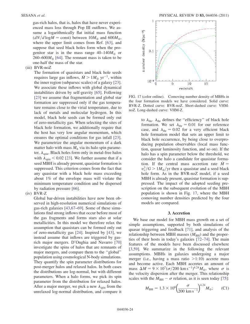
gas-rich halos, that is, halos that have never experi-enced mass loss through Pop III outflows. We as-sume a logarithmically flat initial mass function(dN=d logM ¼ const) between 10M and 600M,where the upper limit comes from Ref. [63], andsuppose that seed black holes form when the pro-genitor star is in the mass range 40–140M or260–600M [64]. The remnant mass is taken to beone-half the mass of the star.

(iii) BVR-noZThe formation of quasistars and black hole seedsrequires large gas inflows, _M> 1M yr1, withinthe inner region (subparsec scales) of a galaxy [23].We associate these inflows with global dynamicalinstabilities driven by self-gravity [65]. Following[23] we assume that fragmentation and global starformation are suppressed only if the gas tempera-ture remains close to the virial temperature, due tolack of metals and molecular hydrogen. In thismodel, black hole seeds can be formed only outof zero-metallicity gas. When selecting the sites ofblack hole formation, we additionally require thatthe host has very low angular momentum, whichensures the optimal conditions for gas infall [23].We parametrize the angular momentum of a darkmatter halo with massMh via its halo spin parame-ter, spin. Black holes form only in metal-free halos

with spin < 0:02 [23]. We further assume that if a

seed MBH is already present, quasistar formation issuppressed. This criterion comes from the fact thatany quasistar with a black hole mass exceedingabout 1% of the envelope mass will violate theminimum temperature condition and be dispersedby radiation pressure [66].

(iv) BVR-ZGlobal bar-driven instabilities have now been ob-served in high-resolution numerical simulations ofgas-rich galaxies [43,67–69]. Some of these simu-lations find strong inflows that occur before most ofthe gas fragments and forms stars also at solarmetallicities. In this model we therefore relax theassumption that quasistars can be formed only outof zero-metallicity gas [24]. Inspired by [43], weinstead assume that inflows are triggered by gas-rich major mergers. D’Onghia and Navarro [70]investigate the spins of halos that are remnants ofmajor mergers, and compare them to the ‘‘global’’population using cosmological N-body simulations.They quantify the spin parameter distributions forpost-merger halos and relaxed halos. In both casesthe distributions are log-normal, but with differentparameters. When a halo forms, we pick its spinparameter from the distribution for relaxed halos.After a major merger, we pick a new spin from the

unrelaxed log-normal distribution, and compare it

to thr. thr defines the ‘‘efficiency’’ of black holeformation. We set thr ¼ 0:01 for our referencecase, and thr ¼ 0:02 for a very efficient blackhole formation model that sets an upper limit toblack hole occurrence, by being close to overpro-ducing population observables (local mass func-tion, quasar luminosity function, and so on). If thehalo has a spin parameter below the threshold, weconsider the halo a candidate for quasistar forma-tion. If the central mass accretion rate _M ¼v3c=G> 1M=yr then a quasistar and a seed black

hole form. As in the BVR-noZ model, if a seedMBH is already present, quasistar formation is sup-pressed. The impact of the adopted seeding pre-scription on the subsequent evolution of the MBHpopulation is shown in Fig. 17, where the MBHcomoving number densities predicted by the fourmodels are compared.

3. Accretion

We base our model for MBH mass growth on a set ofsimple assumptions, supported by both simulations ofquasar triggering and feedback [71], and analysis of therelationship between MBH masses (MBH) and the proper-ties of their hosts in today’s galaxies [72–74]. The mainfeatures of the models have been discussed elsewhere[3,59]. We summarize in the following the relevantassumptions. MBHs in galaxies undergoing a majormerger (i.e., having a mass ratio >1:10) accrete massand become active. Each MBH accretes an amount ofmass M ¼ 9 107ð=200 km s1Þ4:24M, where isthe velocity dispersion after the merger. This relationshipscales with the MBH relation, as it is seen today [75]:

MBH ¼ 1:3 108

200 km s1

4:24

M; (C1)

FIG. 17 (color online). Comoving number density of MBHs inthe four formation models we have considered. Solid curve:BVR-Z. Dotted curve: BVR-noZ. Short-dashed curve: VHM-noZ. Long-dashed curve: VHM-Z.


044036-24

the normalization in M was chosen to take into accountthe contribution of mergers, without exceeding the massgiven by the MBH relation.

We link the central stellar velocity dispersion of the host,i.e. in Eq. (C1), to the asymptotic circular velocity (vc)

as ¼ vc=ffiffiffi3

p, assuming orbital isotropy [74,76,77]. The

asymptotic circular velocity is a measure of the total massof the dark matter halo of the host galaxy. We calculate thecircular velocity from the mass of the host halo and itsredshift [24].

The rate at which mass is accreted scales with theEddington rate for the MBH, and we set either a fixedEddington ratio of fEdd ¼ 1, or an accretion rate derivedfrom the distribution discussed in [44]. Accretion startsafter a dynamical time scale and lasts until the MBH, ofinitial mass Min, has accreted a mass M. The lifetime ofan AGN therefore depends on how much mass it accretesduring each episode:

tAGN ¼ tEddfEdd

1 lnðMfin=MinÞ; (C2)

where is the radiative efficiency ( ’ 0:1),tEdd ¼ 0:45 Gyr and Mfin ¼ min½ðMin þ MÞ; 1:3108ð=200 km s1Þ4:24M.We further assume that, when two galaxies hosting

MBHs merge, the MBHs themselves merge within themerger time scale of the host halos, which is a plausibleassumption for MBH binaries formed after gas-richgalaxy mergers [78]. We adopt the relations suggestedby Ref. [79] for the merger time scale. Black holes areallowed to accrete during the merging process if the timescale for accretion, corresponding to the sum of the dy-namical time scale and tAGN, is longer than the merger timescale.

[1] S. D.M. White and M. J. Rees, Mon. Not. R. Astron. Soc.

183, 341 (1978).[2] G. Kauffmann and M. Haehnelt, Mon. Not. R. Astron.

Soc. 311, 576 (2000).[3] M. Volonteri, F. Haardt, and P. Madau, Astrophys. J. 582,

559 (2003).[4] Z. Haiman and K. Menou, Astrophys. J. 531, 42 (2000).[5] G. Kauffmann and M. Haehnelt, Mon. Not. R. Astron.

Soc. 311, 576 (2000).[6] J. S. B. Wyithe and A. Loeb, Astrophys. J. 595, 614

(2003).[7] D. J. Croton et al., Mon. Not. R. Astron. Soc. 356, 1155

(2005).[8] R. K. Malbon, C.M. Baugh, C. S. Frenk, and C.G. Lacey,

Mon. Not. R. Astron. Soc. 382, 1394 (2007).[9] T. Di Matteo, J. Colberg, V. Springel, L. Hernquist, and D.

Sijacki, Astrophys. J. 676, 33 (2008).[10] J. Magorrian et al., Astron. J. 115, 2285 (1998).[11] S. Gillessen et al., Astrophys. J. Lett. 707, L114 (2009).[12] S. A. Hughes, Mon. Not. R. Astron. Soc. 331, 805 (2002).[13] K. G. Arun et al., Classical Quantum Gravity 26, 094027

(2009).[14] E. Berti, V. Cardoso, and C.M. Will, Phys. Rev. D 73,

064030 (2006).[15] S. T. McWilliams, J. I. Thorpe, J. G. Baker, and B. J. Kelly,

Phys. Rev. D 81, 064014 (2010).[16] D. E. Holz and S.A. Hughes, Astrophys. J. 629, 15

(2005).[17] K. G. Arun, B. R. Iyer, B. S. Sathyaprakash, S. Sinha, and

C.V. D. Broeck, Phys. Rev. D 76, 104016 (2007).[18] C. Van Den Broeck, M. Trias, B. S. Sathyaprakash, and

A.M. Sintes, Phys. Rev. D 81, 124031 (2010).[19] S. Hilbert, J. R. Gair, and L. J. King, arXiv:1007.2468.[20] S. Babak, J. R. Gair, A. Petiteau, and A. Sesana,

arXiv:1011.2062.

[21] S.M. Koushiappas, J. S. Bullock, and A. Dekel, Mon. Not.

R. Astron. Soc. 354, 292 (2004).[22] G. Lodato and P. Natarajan, Mon. Not. R. Astron. Soc.

371, 1813 (2006).[23] M. C. Begelman, M. Volonteri, and M. J. Rees, Mon. Not.

R. Astron. Soc. 370, 289 (2006).[24] M. Volonteri and M.C. Begelman, Mon. Not. R. Astron.

Soc. 409, 1022 (2010).[25] J. S. B. Wyithe and A. Loeb, Astrophys. J. 590, 691

(2003).[26] A. Sesana, F. Haardt, P. Madau, and M. Volonteri,

Astrophys. J. 611, 623 (2004).[27] A. Sesana, F. Haardt, P. Madau, and M. Volonteri,

Astrophys. J. 623, 23 (2005).[28] A. Sesana, M. Volonteri, and F. Haardt, Mon. Not. R.

Astron. Soc. 377, 1711 (2007).[29] M. Enoki, K. T. Inoue, M. Nagashima, and N. Sugiyama,

Astrophys. J. 615, 19 (2004).[30] K. J. Rhook and J. S. B. Wyithe, Mon. Not. R. Astron. Soc.

361, 1145 (2005).[31] J. E. Plowman, D. C. Jacobs, R.W. Hellings, S. L. Larson,

and S. Tsuruta, Mon. Not. R. Astron. Soc. 401, 2706

(2010).[32] J. E. Plowman, R.W. Hellings, and S. Tsuruta,

arXiv:1009.0765.[33] J. R. Gair, A. Sesana, E. Berti, and M. Volonteri,

‘‘Constraining Properties of the Black Hole Population

Using LISA,’’ Classical Quantum Gravity (to be pub-

lished).[34] E. S. Phinney et al., in The Big Bang Observer: Direct

Detection of Gravitational Waves from the Birth of the

Universe to the Present, NASA Mission Concept Study

(2004).[35] J. Crowder and N. J. Cornish, Phys. Rev. D 72, 083005

(2005).


044036-25

http://dx.doi.org/10.1046/j.1365-8711.2000.03077.x

http://dx.doi.org/10.1046/j.1365-8711.2000.03077.x

http://dx.doi.org/10.1086/344675

http://dx.doi.org/10.1086/344675

http://dx.doi.org/10.1086/308468

http://dx.doi.org/10.1046/j.1365-8711.2000.03077.x

http://dx.doi.org/10.1046/j.1365-8711.2000.03077.x

http://dx.doi.org/10.1086/377475

http://dx.doi.org/10.1086/377475

http://dx.doi.org/10.1111/j.1365-2966.2004.08546.x

http://dx.doi.org/10.1111/j.1365-2966.2004.08546.x

http://dx.doi.org/10.1086/524921

http://dx.doi.org/10.1086/300353

http://dx.doi.org/10.1088/0004-637X/707/2/L114

http://dx.doi.org/10.1046/j.1365-8711.2002.05247.x

http://dx.doi.org/10.1088/0264-9381/26/9/094027

http://dx.doi.org/10.1088/0264-9381/26/9/094027




http://dx.doi.org/10.1086/431341

http://dx.doi.org/10.1086/431341



http://arXiv.org/abs/1007.2468


http://dx.doi.org/10.1111/j.1365-2966.2004.08190.x

http://dx.doi.org/10.1111/j.1365-2966.2004.08190.x

http://dx.doi.org/10.1111/j.1365-2966.2006.10801.x

http://dx.doi.org/10.1111/j.1365-2966.2006.10801.x

http://dx.doi.org/10.1111/j.1365-2966.2010.17359.x

http://dx.doi.org/10.1111/j.1365-2966.2010.17359.x

http://dx.doi.org/10.1086/375187

http://dx.doi.org/10.1086/375187

http://dx.doi.org/10.1086/422185

http://dx.doi.org/10.1086/428492

http://dx.doi.org/10.1111/j.1365-2966.2007.11734.x

http://dx.doi.org/10.1111/j.1365-2966.2007.11734.x

http://dx.doi.org/10.1086/424475

http://dx.doi.org/10.1111/j.1365-2966.2005.08987.x

http://dx.doi.org/10.1111/j.1365-2966.2005.08987.x

http://dx.doi.org/10.1111/j.1365-2966.2009.15853.x

http://dx.doi.org/10.1111/j.1365-2966.2009.15853.x




[36] M. Ando et al., Classical Quantum Gravity 27, 084010(2010).

[37] E. Berti and M. Volonteri, Astrophys. J. 684, 822 (2008).[38] S. Tremaine et al., Astrophys. J. 574, 740 (2002).[39] P. Madau and M. J. Rees, Astrophys. J. Lett. 551, L27

(2001).[40] I. Shlosman, J. Frank, and M. C. Begelman, Nature

(London) 338, 45 (1989).[41] V. Bromm and A. Loeb, Astrophys. J. 596, 34 (2003).[42] E. Scannapieco, R. Schneider, and A. Ferrara, Astrophys.

J. 589, 35 (2003).[43] L. Mayer, S. Kazantzidis, A. Escala, and S. Callegari,

Nature (London) 466, 1082 (2010).[44] A. Merloni and S. Heinz, Mon. Not. R. Astron. Soc. 388,

1011 (2008).[45] A. Toomre, Astrophys. J. 139, 1217 (1964).[46] A. R. King and J. E. Pringle, Mon. Not. R. Astron. Soc.

373, L90 (2006).[47] E. Berti, A. Buonanno, and C.M. Will, Phys. Rev. D 71,

084025 (2005).[48] E. Berti, A. Buonanno, and C.M. Will, Classical Quantum

Gravity 22, S943 (2005).[49] C. Cutler, Phys. Rev. D 57, 7089 (1998).[50] E. Berti et al., Phys. Rev. D 76, 064034 (2007).[51] S. T. McWilliams, B. J. Kelly, and J. G. Baker, Phys. Rev.

D 82, 024014 (2010).[52] M. Vallisneri, Phys. Rev. D 77, 042001 (2008).[53] J. R. Gair, C. Tang, and M. Volonteri, Phys. Rev. D 81,

104014 (2010).[54] D. J. C. Mackay, Information Theory, Inference and

Learning Algorithms, (Cambridge University Press,Cambridge, England, 2003).

[55] Y. Wang, D. E. Holz, and D. Munshi, Astrophys. J. Lett.572, L15 (2002).

[56] E. Komatsu et al., Astrophys. J. Suppl. Ser. 180, 330(2009).

[57] M. Volonteri, P. Madau, E. Quataert, and M. J. Rees,Astrophys. J. 620, 69 (2005).

[58] M. Volonteri, J.M. Miller, and M. Dotti, Astrophys. J. 703,86 (2009).

[59] M. Volonteri and P. Natarajan, Mon. Not. R. Astron. Soc.400, 1911 (2009).

[60] E. Scannapieco, R. Schneider, and A. Ferrara, Astrophys.J. 589, 35 (2003).

[61] E. Scannapieco and R. Barkana, Astrophys. J. 571, 585(2002).

[62] N. Yoshida, K. Omukai, L. Hernquist, and T. Abel,Astrophys. J. 652, 6 (2006).

[63] K. Omukai and F. Palla, Astrophys. J. 589, 677 (2003).[64] C. L. Fryer, S. E. Woosley, and A. Heger, Astrophys. J.

550, 372 (2001).[65] I. Shlosman, J. Frank, and M.C. Begelman, Nature

(London) 338, 45 (1989).[66] M. C. Begelman, E.M. Rossi, and P. J. Armitage, Mon.

Not. R. Astron. Soc. 387, 1649 (2008).[67] J. H. Wise, M. J. Turk, and T. Abel, Astrophys. J. 682, 745

(2008).[68] R. Levine, N.Y. Gnedin, A. J. S. Hamilton, and A.V.

Kravtsov, Astrophys. J. 678, 154 (2008).[69] J. A. Regan and M.G. Haehnelt, Mon. Not. R. Astron.

Soc. 396, 343 (2009).[70] E. D’Onghia and J. F. Navarro, Mon. Not. R. Astron. Soc.

380, L58 (2007).[71] V. Springel, T. Di Matteo, and L. Hernquist, Astrophys. J.

620, L79 (2005).[72] K. Gebhardt et al., Astrophys. J. 539, L13 (2000).[73] L. Ferrarese and D. Merritt, Astrophys. J. 539, L9 (2000).[74] L. Ferrarese, Astrophys. J. 578, 90 (2002).[75] K. Gultekin et al., Astrophys. J. 698, 198 (2009).[76] A. Pizzella et al., Astrophys. J. 631, 785 (2005).[77] M. Baes, P. Buyle, G.K. T. Hau, and H. Dejonghe, Mon.

Not. R. Astron. Soc. 341, L44 (2003).[78] M. Dotti, M. Colpi, F. Haardt, and L. Mayer, Mon. Not. R.

Astron. Soc. 379, 956 (2007).[79] G. Taffoni, L. Mayer, M. Colpi, and F. Governato, Mon.

Not. R. Astron. Soc. 341, 434 (2003).


044036-26

http://dx.doi.org/10.1088/0264-9381/27/8/084010

http://dx.doi.org/10.1088/0264-9381/27/8/084010

http://dx.doi.org/10.1086/590379

http://dx.doi.org/10.1086/341002

http://dx.doi.org/10.1086/319848

http://dx.doi.org/10.1086/319848

http://dx.doi.org/10.1038/338045a0

http://dx.doi.org/10.1038/338045a0

http://dx.doi.org/10.1086/377529

http://dx.doi.org/10.1086/374412

http://dx.doi.org/10.1086/374412

http://dx.doi.org/10.1038/nature09294

http://dx.doi.org/10.1086/147861

http://dx.doi.org/10.1111/j.1745-3933.2006.00249.x

http://dx.doi.org/10.1111/j.1745-3933.2006.00249.x



http://dx.doi.org/10.1088/0264-9381/22/18/S08

http://dx.doi.org/10.1088/0264-9381/22/18/S08








http://dx.doi.org/10.1086/341604

http://dx.doi.org/10.1086/341604

http://dx.doi.org/10.1088/0067-0049/180/2/330

http://dx.doi.org/10.1088/0067-0049/180/2/330

http://dx.doi.org/10.1086/426858

http://dx.doi.org/10.1088/0004-637X/703/1/L86

http://dx.doi.org/10.1088/0004-637X/703/1/L86

http://dx.doi.org/10.1111/j.1365-2966.2009.15577.x

http://dx.doi.org/10.1111/j.1365-2966.2009.15577.x

http://dx.doi.org/10.1086/374412

http://dx.doi.org/10.1086/374412

http://dx.doi.org/10.1086/340063

http://dx.doi.org/10.1086/340063

http://dx.doi.org/10.1086/507978

http://dx.doi.org/10.1086/374810

http://dx.doi.org/10.1086/319719

http://dx.doi.org/10.1086/319719

http://dx.doi.org/10.1038/338045a0

http://dx.doi.org/10.1038/338045a0

http://dx.doi.org/10.1111/j.1365-2966.2008.13344.x

http://dx.doi.org/10.1111/j.1365-2966.2008.13344.x

http://dx.doi.org/10.1086/588209

http://dx.doi.org/10.1086/588209

http://dx.doi.org/10.1086/529064

http://dx.doi.org/10.1111/j.1365-2966.2009.14579.x

http://dx.doi.org/10.1111/j.1365-2966.2009.14579.x

http://dx.doi.org/10.1111/j.1745-3933.2007.00348.x

http://dx.doi.org/10.1111/j.1745-3933.2007.00348.x

http://dx.doi.org/10.1086/428772

http://dx.doi.org/10.1086/428772

http://dx.doi.org/10.1086/312840

http://dx.doi.org/10.1086/312838

http://dx.doi.org/10.1086/342308

http://dx.doi.org/10.1088/0004-637X/698/1/198

http://dx.doi.org/10.1086/430513

http://dx.doi.org/10.1046/j.1365-8711.2003.06680.x

http://dx.doi.org/10.1046/j.1365-8711.2003.06680.x

http://dx.doi.org/10.1111/j.1365-2966.2007.12010.x

http://dx.doi.org/10.1111/j.1365-2966.2007.12010.x

http://dx.doi.org/10.1046/j.1365-8711.2003.06395.x

http://dx.doi.org/10.1046/j.1365-8711.2003.06395.x

PHYSICAL REVIEW D 044036 (2011) Reconstructing the …pubman.mpdl.mpg.de/pubman/item/escidoc:1313725/component/esci… · Reconstructing the massive black hole cosmic history through

Documents