Physica D Data-driven approximation of the Koopman generator

Physica D 406 (2020) 132416

Contents lists available at ScienceDirect

Physica D

journal homepage: www.elsevier.com/locate/physd

Data-driven approximation of the Koopman generator:Modelreduction, system identification, and controlStefan Klus a,∗, Feliks Nüske b,c, Sebastian Peitz c, Jan-Hendrik Niemann d,Cecilia Clementi b, Christof Schütte a,d

a Department of Mathematics and Computer Science, Freie Universität Berlin, Germanyb Center for Theoretical Biological Physics and Department of Chemistry, Rice University, USAc Department of Mathematics, Paderborn University, Germanyd Zuse Institute Berlin, Germany

a r t i c l e i n f o

Article history:Received 23 September 2019Received in revised form 7 February 2020Accepted 12 February 2020Available online 15 February 2020

Keywords:Data-driven methodsKoopman operatorInfinitesimal generatorSystem identificationCoarse grainingControl

a b s t r a c t

We derive a data-driven method for the approximation of the Koopman generator called gEDMD, whichcan be regarded as a straightforward extension of EDMD (extended dynamic mode decomposition). Thisapproach is applicable to deterministic and stochastic dynamical systems. It can be used for computingeigenvalues, eigenfunctions, and modes of the generator and for system identification. In additionto learning the governing equations of deterministic systems, which then reduces to SINDy (sparseidentification of nonlinear dynamics), it is possible to identify the drift and diffusion terms of stochasticdifferential equations from data. Moreover, we apply gEDMD to derive coarse-grained models of high-dimensional systems, and also to determine efficient model predictive control strategies. We highlightrelationships with other methods and demonstrate the efficacy of the proposed methods using severalguiding examples and prototypical molecular dynamics problems.

© 2020 Elsevier B.V. All rights reserved.

1. Introduction

Data-driven approaches for the analysis of complex dynamicalsystems – be it methods to approximate transfer operators forcomputing metastable or coherent sets, methods to learn phys-ical laws, or methods for optimization and control – have beensteadily gaining popularity over the last years. Algorithms suchas DMD [1,2], EDMD [3,4], SINDy [5], and their various kernel-[3,6,7], tensor- [8–10], or neural network-based [11–13] exten-sions and generalizations have been successfully applied to aplethora of different problems, including molecular and fluid dy-namics, meteorology, finance, as well as mechanical and electricalengineering. An overview of different applications can be found,e.g., in [14]. Similar methods, developed mainly for reversiblemolecular dynamics problems, have been proposed in [15]. Mostof the aforementioned techniques turn out to be strongly re-lated, with the unifying concept being Koopman operator theory[16–18]. In what follows, we will focus mainly on the generatorof the Koopman operator and its properties and applications.

SINDy [5] constitutes a milestone for data-driven discovery ofdynamical systems. Because of the close relationship between thevector field of a deterministic dynamical system and its Koopman

∗ Corresponding author.E-mail address: [email protected] (S. Klus).

generator, SINDy is a special case of the framework we will intro-duce in this study. In [19,20], an extension of SINDy to determineeigenfunctions of the Koopman generator was presented. Thediscovered eigenfunctions are then used for control, resulting inthe so-called KRONIC framework. Another extension of SINDywas derived in [21], allowing for the identification of parametersof a stochastic system using Kramers–Moyal formulae.

A different avenue towards system identification was takenin [22,23]. Here, the Koopman operator is first approximated withthe aid of EDMD, and then its generator is determined using thematrix logarithm. Subsequently, the right-hand side of the differ-ential equation is extracted from the matrix representation of thegenerator. The relationship between the Koopman operator andits generator was also exploited in [24] for parameter estimationof stochastic differential equations.

A method for computing eigenfunctions of the Koopman gen-erator was proposed in [25], where the diffusion maps algorithmis used to set up a Galerkin-projected eigenvalue problem withorthogonal basis elements. Two efficient methods for computingthe generator of the adjoint Perron–Frobenius operator based onUlam’s method and spectral collocation were presented in [26].Provided that a model of the system dynamics is available, thecomputation of trajectories can be replaced by evaluations of theright-hand side of the system, which is often orders of magnitudefaster.

https://doi.org/10.1016/j.physd.2020.1324160167-2789/© 2020 Elsevier B.V. All rights reserved.

2 S. Klus, F. Nüske, S. Peitz et al. / Physica D 406 (2020) 132416

The purpose of this study is to present a general framework tocompute a matrix approximation of the Koopman generator, bothfor deterministic and stochastic systems, and to explore a rangeof applications. The main contributions of this work are:

1. We reformulate standard EDMD in such a way that it canbe used to approximate the generator of the Koopmanoperator – as well as its eigenvalues, eigenfunctions, andmodes – from data without resorting to trajectory integra-tion. Exploiting duality, this can be extended naturally tothe generator of the Perron–Frobenius operator.

2. We illustrate that the governing equations of deterministicas well as stochastic dynamical systems can be obtainedfrom empirical estimates of the generator. Furthermore, wehighlight relationships with related system identificationtechniques such as the Koopman lifting approach [22],SINDy [5], and KRONIC [19], which focus mainly on identi-fying ordinary differential equations.

3. Lastly, we explore two powerful applications of the approx-imated Koopman generator. We show that gEDMD can beused to identify coarse-grained models based on data of thefull system, which is a highly relevant topic across differentresearch fields, like molecular dynamics simulations forinstance. Moreover, we apply the Koopman generator tocontrol dynamical systems, providing flexible and efficientmodel predictive control strategies.

The efficacy of the resulting methods will be demonstratedwith the aid of guiding examples and illustrative benchmarkproblems.

The remainder of this paper is structured as follows: In Sec-tion 2, we introduce the Koopman operator and its generatorfor different kinds of dynamical systems. We then derive anextension of EDMD for the approximation of the Koopman gen-erator, named gEDMD, in Section 3. Furthermore, relationshipswith other methods are described. Section 4 explores additionalapplications of the proposed methods, namely coarse-grainingand the application to control problems. Open questions andfuture work are discussed in Section 5.

2. The Koopman operator and its generator

In what follows, let X be the state space, e.g., X ⊂ Rd, andf ∈ L∞(X) a real-valued observable of the system.

2.1. Deterministic dynamical systems

Given an ordinary differential equation of the form x = b(x),where b:Rd

→ Rd, the so-called Koopman semigroup of operators{Kt

} is defined as

(Kt f )(x) = f (Φ t (x)),

whereΦ t is the flowmap, see [4,17,18]. That is, if x(t) is a solutionof the initial value problem with initial condition x(0) = x0, thenΦ t (x0) = x(t). The infinitesimal generator L of the semigroup,defined as

Lf = limt→0

1t

(Kt f − f

),

is given by

Lf =ddt

f = b · ∇xf =

d∑i=1

bi∂ f∂xi,

see, e.g., [17]. Thus, if f is continuously differentiable, thenu(t, x) = Kt f (x) satisfies the first-order partial differential equa-tion ∂u

∂t = Lu. The adjoint operator L∗, i.e., the generator of the

Perron–Frobenius operator, is given by

L∗f = −

d∑i=1

∂(bi f )∂xi

.

Example 2.1. Throughout the paper, we will use the simplesystem

x1 = γ x1,

x2 = δ (x2 − x21),

taken from [27], as a guiding example. In addition to the trivialeigenfunction ϕ1(x) = 1 with corresponding generator eigenvalueλ1 = 0, we obtain ϕ2(x) = x1 and ϕ3(x) =

2γ−δ

δx2 + x21

with corresponding generator eigenvalues λ2 = γ and λ3 =

δ, respectively. Moreover, products of eigenfunctions are againeigenfunctions. △

2.2. Non-deterministic dynamical systems

Similarly, the definition of the Koopman operator can be gen-eralized to stochastic differential equations

dXt = b(Xt ) dt + σ (Xt ) dWt (1)

as described, e.g., in [28], resulting in

(Kt f )(x) = E[f (Φ t (x))]. (2)

Here, E[ · ] denotes the expected value, b:Rd→ Rd is the

drift term, σ :Rd→ Rd×s the diffusion term, and Wt an s-

dimensional Wiener process. Given a twice continuously differ-entiable function f , it can be shown using Itô’s lemma that theinfinitesimal generator of the stochastic Koopman operator isthen characterized by

Lf = b · ∇xf +12a : ∇

2x f =

d∑i=1

bi∂ f∂xi

+12

d∑i=1

d∑j=1

aij∂2f∂xi ∂xj

, (3)

where a = σ σ⊤ and ∇2x denotes the Hessian. Properties of

the generator associated with non-deterministic dynamical sys-tems are studied in [29]. The function u(t, x) = Kt f (x) satisfiesthe second-order partial differential equation ∂u

∂t = Lu, whichis called the Kolmogorov backward equation [30]. The adjointoperator in this case is

L∗f = −

d∑i=1

∂(bi f )∂xi

+12

d∑i=1

d∑j=1

∂2(aij f )∂xi ∂xj

so that ∂u∂t = L∗u becomes the Fokker–Planck equation or Kol-

mogorov forward equation [17].If µ is a stationary measure for the process Xt , the Koopman

operator can be extended from L∞µ (X) to the Hilbert space L2µ(X)

with inner product ⟨f , g⟩µ =∫X f (x) g(x) dµ(x) [31]. We will

frequently consider this situation in what follows. An importantclass of stochastic differential equations are those which arereversible with respect to a measure µ, which is necessarily astationary measure in this case. The Koopman operator becomesself-adjoint on L2µ(X) in the reversible setting. Reversible systemscan be characterized by the diffusion σ and a scalar potentialF :Rd

→ R, from which the drift is then obtained by

b = −12a∇F +

12∇ · a,

where the divergence in the second term is applied to each col-umn of a [32]. The generator of a reversible stochastic differentialequation is a self-adjoint and typically unbounded operator on asuitable dense subspace of L2µ(X).

S. Klus, F. Nüske, S. Peitz et al. / Physica D 406 (2020) 132416 3

Remark 2.2. For systems of the form dXt = −∇V (Xt ) dt +√2β−1 dWt , which play an important role in molecular dynamics,

we obtain

Lf = −∇V ·∇f +β−1∆f and L∗f = ∇V ·∇f +∆V f +β−1∆f .

Here, V describes the potential and β is the inverse temperature.The resulting dynamics are reversible with invariant measureµ(x) ∼ exp(−β V (x)). The generator L is self-adjoint on L2µ(X)and it can be shown that, assuming suitable growth conditionson the potential, the spectrum of L is discrete [33].

Example 2.3. We will use the one-dimensional Ornstein–Uhlenbeck process, given by the stochastic differential equation

dXt = −α Xt dt +

√2β−1 dWt ,

which is of the above form with V (x) =12 α x2, as a second

guiding example. The parameter α is the friction coefficient. Thegenerator becomes self-adjoint in the space L2(ρ) weighted by theinvariant density

ρ(x) =1√

2πα−1β−1exp

(−α β

x2

2

)and the eigenvalues λℓ and eigenfunctions ϕℓ are given by

λℓ = −α (ℓ−1), ϕℓ(x) =1

√(ℓ− 1)!

Hℓ−1

(√αβ x

), ℓ = 1, 2, . . . ,

where Hℓ denotes the ℓth probabilists’ Hermite polynomial [32].That these functions are indeed eigenfunctions can be verifiedeasily using recurrence relations for the Hermite polynomials,i.e., Hℓ+1(x) = xHℓ(x) − H ′

ℓ(x). △

2.3. Galerkin approximation

Given a set of basis functions {ψi}ni=1, where ψi:Rd

→ R, aGalerkin approximation L of the generator L can be obtained bycomputing the matrices A,G ∈ Rn×n with

Aij =⟨Lψi, ψj

⟩µ,

Gij =⟨ψi, ψj

⟩µ,

(4)

where µ is a given measure. The matrix representation L ofthe projected operator L is then given by L⊤

= AG−1. Wedefine ψ(x) = [ψ1(x), . . . , ψn(x)]⊤. That is, for a function f (x) =∑n

i=1 ci ψi(x) = c⊤ψ(x), it holds that (Lf )(x) = (L c)⊤ψ(x), wherec = [c1, . . . , cn]⊤ ∈ Rn. It follows that an eigenvector ξℓ of Lcorresponding to the eigenvalue λℓ contains the coefficients forthe eigenfunctions of L since defining ϕℓ(x) = ξ⊤

ℓ ψ(x) yields

(Lϕℓ)(x) = (L ξℓ)⊤ψ(x) = λℓ ξ⊤

ℓ ψ(x) = λℓ ϕℓ(x).

In many applications, the reciprocals of the generator eigenvalues(or their approximations) are also of interest, as they can beinterpreted as decay time scales of dynamical processes in thesystem. We will refer to them as implied time scales

tℓ :=1λℓ.

Example 2.4. For the Ornstein–Uhlenbeck process and a ba-sis comprising monomials of order up to n − 1, i.e., ψ(x) =

[1, x, . . . , xn−1]⊤, we can compute the matrix L analytically. Note

that Lψk is again in the subspace spanned by {ψi}ni=1. In particular,

for k ≥ 3, we have

(Lψk)(x) = −α (k − 1) xk−1+ β−1(k − 1)(k − 2) xk−3

and the matrix L ∈ Rn×n is of the form

⎡⎢⎢⎢⎢⎢⎢⎢⎢⎢⎢⎢⎣

1 x x2 x3 x4 x5 x6 ...

1 0 2β−1

x −α 6β−1

x2 −2α 12β−1

x3 −3α 20β−1

x4 −4α 30β−1

x5 −5α. . .

x6 −6α...

. . .

⎤⎥⎥⎥⎥⎥⎥⎥⎥⎥⎥⎥⎦,

where the row and column labels correspond to the respectivebasis functions. The eigenvalues of the generator are given byλℓ = −α (ℓ−1), for ℓ = 1, . . . , n, and the resulting eigenfunctionswhose coefficients are given by the eigenvectors are the (trans-formed) probabilists’ Hermite polynomials as described above.An approach to compute Hermite polynomials by solving aneigenvalue problem, resulting in a similar matrix representation,is also described in [34]. △

Since we in general cannot compute the required integrals an-alytically, the aim is to estimate them from data using, e.g., MonteCarlo integration. More details regarding different types of Galer-kin approximations and other methods for the approximation oftransfer operators from data can be found in [4,35].

Remark 2.5. Issues pertaining to non-compactness or continuousspectra of Koopman operators associated with systems of highcomplexity are beyond the scope of this paper. Although suchcases can theoretically be handled, the numerical analysis is oftenchallenging and typically requires regularization, which is, forinstance, implicitly given by Galerkin projections [25]. This isdiscussed in detail in the aforecited work by Giannakis. Moreover,the projected generator does in general not result in a rate ma-trix, see [36,37] for details on Galerkin discretizations of transferoperators and their properties.

3. Infinitesimal generator EDMD

EDMD [4,38] was developed for the approximation of theKoopman or Perron–Frobenius operator from data. However, itcan be reformulated to compute also the associated infinitesimalgenerators. We will call the resulting method gEDMD.

3.1. Deterministic dynamical systems

Let us first consider the deterministic case, which – albeitderived in another way and with different applications in mind– has already been studied in [19,20] so that we only brieflysummarize and extend these results and then generalize them tothe non-deterministic setting. Detailed relationships with othermethods can be found in Section 3.3. We now assume that wehavemmeasurements of the states of the system, given by {xl}ml=1,and the corresponding time derivatives, given by {xl}ml=1. Thederivatives might also be estimated from data, cf. [5].

3.1.1. Generator approximationSimilar to the Galerkin projection described above, we then

choose a set of basis functions, also sometimes called dictionary,defined by {ψi}

ni=1, and write this again in vector form as ψ(x) =

[ψ1(x), . . . , ψn(x)]⊤. Additionally, we define

ψk(x) = (Lψk)(x) =

d∑i=1

bi(x)∂ψk

∂xi(x).

4 S. Klus, F. Nüske, S. Peitz et al. / Physica D 406 (2020) 132416

For all data points and basis functions, this can be written inmatrix form as

ΨX =

⎡⎢⎣ψ1(x1) . . . ψ1(xm)...

. . ....

ψn(x1) . . . ψn(xm)

⎤⎥⎦ and

ΨX =

⎡⎢⎣ψ1(x1) . . . ψ1(xm)...

. . ....

ψn(x1) . . . ψn(xm)

⎤⎥⎦ ,where ΨX , ΨX ∈ Rn×m. The partial derivatives of the basis func-tions required for ψk(xl) can be precomputed analytically.1 Notethat we additionally need b(xl) which is simply xl. If the timederivatives cannot be measured directly, they can be approxi-mated using, e.g., finite differences. We now assume there existsa matrix M such that ΨX = MΨX . Since this equation in gen-eral cannot be satisfied exactly, we solve it in the least squaressense – analogously to the derivation of EDMD – by minimizing∥ΨX − MΨX∥F , resulting in

M = ΨXΨ+

X =(ΨXΨ

⊤

X

)(ΨXΨ

⊤

X

)+= A G+,

with

A =1m

m∑l=1

ψ(xl)ψ(xl)⊤ and G =1m

m∑l=1

ψ(xl)ψ(xl)⊤.

We call this approach gEDMD. The advantage is that the generatormight be sparse even when the Koopman operator for the time-tmap is not.

Remark 3.1. The sparsification approach proposed for SINDy,see [5], can be added in the same way to gEDMD in order tominimize the number of spurious nonzero entries caused, forinstance, by the numerical approximation of the time derivativesor by noisy data.

The convergence to the Galerkin approximation in the infinitedata limit will be shown for the non-deterministic case, thedeterministic counterpart follows as a special case. The matrixM is thus an empirical estimate of L⊤ and we write M = L⊤

=

A G+. Accordingly, exploiting duality, the matrix representationof the adjoint operator L∗, the generator of the Perron–Frobeniusoperator, is given by M∗

= (L∗)⊤ = A ⊤G+. A detailed derivationfor standard EDMD, which can be carried over to gEDMD, can befound in [4]. The convergence of the standard EDMD approxima-tion to the Koopman operator as the number of basis functionsgoes to infinity is discussed in [39]. Whether the results can beextended to gEDMD will be studied in future work.

Example 3.2. Let us again consider the system defined in Exam-ple 2.1 using monomials up to order 8. We set γ = −0.8 andδ = −0.7 and generate 1000 uniformly distributed test pointsin [−2, 2] × [−2, 2]. Then gEDMD results in eigenvalues and(rescaled) eigenfunctions

λ1 ≈ 0, ϕ1(x) ≈ 1,λ2 ≈ −0.7 = δ, ϕ2(x) = 1.286 x2 + 1.000 x21 ≈

2γ−δ

δx2 + x21,

λ3 ≈ −0.8 = γ , ϕ3(x) ≈ x1.

The subsequent eigenfunctions are products of the above eigen-functions, we obtain, for instance, λ6 ≈ −1.6 = 2 γ with ϕ6(x) =

1.000 x21 ≈ ϕ3(x)2. Note that the ordering of the eigenvalues,which are typically sorted by decreasing values, and associatedeigenfunctions depends on the values of γ and δ. △

1 Alternatively, automatic differentiation or symbolic computing toolboxescould be utilized.

3.1.2. System identificationWith the aid of the full-state observable g(x) = x, it is possible

to reconstruct the governing equations of the underlying dynam-ical system. Note that X needs to be bounded here – and forthe identification of stochastic differential equations introducedbelow – so that g is (component-wise) contained in L∞(X). Letξℓ be the ℓth eigenvector of L and Ξ = [ξ1, . . . , ξn]. Furthermore,assume that B ∈ Rn×d is the matrix such that g(x) = B⊤ ψ(x). Thiscan be easily accomplished by adding the observables { xi }di=1 tothe dictionary. In order to obtain the Koopman modes for the full-state observable, define ϕ(x) = [ϕ1(x), . . . , ϕn(x)]⊤ = Ξ⊤ψ(x).Then

g(x) = B⊤ ψ(x) = B⊤Ξ−⊤ϕ(x).

The column vectors of the matrix V = B⊤Ξ−⊤ are the Koopmanmodes vℓ. We obtain

(Lg)(x) = b(x) ≈

n∑ℓ=1

λℓ ϕℓ(x)vℓ,

where the generator is applied component-wise. This allows usto decompose a system into different frequencies. The derivationof the modes is equivalent to the standard EDMD case, see [4,38]for more details. Instead of representing the system in terms ofthe eigenvalues, eigenfunctions, and modes of the generator, wecan also express it directly in terms of the basis functions, i.e.,

(Lg)(x) = b(x) ≈ (LB)⊤ ψ(x),

which is then equivalent to SINDy, see Section 3.3.

Example 3.3. Using the eigenvalues λℓ and corresponding eigen-functions ϕℓ(x) as determined in Example 3.2, we can reconstructthe dynamical system from Example 2.1. Only the Koopmanmodes v2 = [0, 0.778]⊤ ≈ [0, δ

2γ−δ]⊤, v3 = [1, 0]⊤, and v6 =

[0, −0.778]⊤ ≈ [0, −δ

2γ−δ]⊤ are required for the reconstruction,

the other modes are numerically zero. That is,

b(x) ≈ λ2 ϕ2(x) v2 + λ3 ϕ3(x) v3 + λ6 ϕ6(x) v6 ≈

[γ x1

δ (x2 − x21)

].

Expressing the system directly in terms of the basis functionsresults in the same representation, the governing equations arehence identified correctly in both cases. △

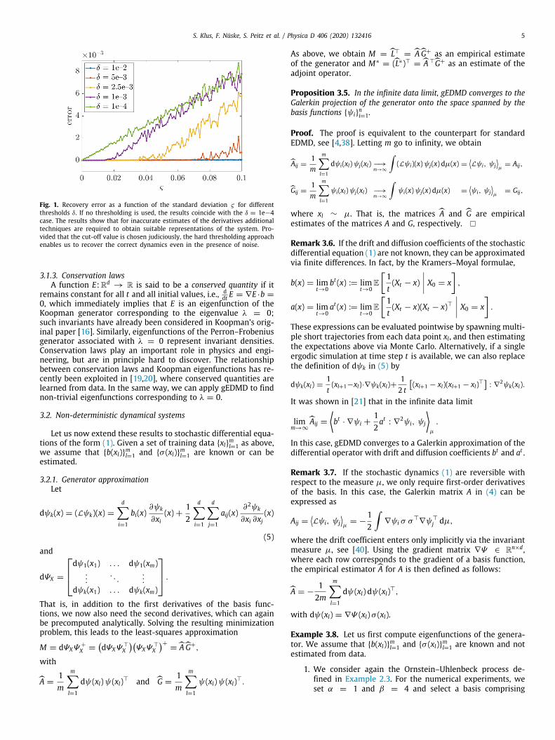
Remark 3.4. In the above example, we assumed that the deriva-tives for the training data are known or can be computed withsufficient accuracy. If the derivatives, however, are noisy or inac-curate, the resulting matrix representations of the operators oftenbecome nonsparse and additional techniques such as denois-ing, total-variation regularization, or iterative hard thresholdingmight be required to eliminate spurious nonzero entries, seealso [5] and references therein. In order to model the presenceof noise, we replace b(xl) by b(xl) + η, where η is sampled froma Gaussian distribution with standard deviation ς . By adding theiterative hard thresholding procedure proposed in [5] to gEDMD,which step by step removes entries larger than a given thresh-old δ and then recomputes the coefficients, we can eliminateunwanted entries. The results, however, depend strongly on thechosen threshold as shown in Fig. 1. The smaller the signal-to-noise ratio, the larger the threshold needs to be to eliminatespurious nonzero entries, but a too large threshold will alsoeliminate the actual coefficients. The error here is defined tobe the average difference between the true and the estimatedcoefficients after 10 iterations of the hard thresholding algorithm.

S. Klus, F. Nüske, S. Peitz et al. / Physica D 406 (2020) 132416 5

Fig. 1. Recovery error as a function of the standard deviation ς for differentthresholds δ. If no thresholding is used, the results coincide with the δ = 1e−4case. The results show that for inaccurate estimates of the derivatives additionaltechniques are required to obtain suitable representations of the system. Pro-vided that the cut-off value is chosen judiciously, the hard thresholding approachenables us to recover the correct dynamics even in the presence of noise.

3.1.3. Conservation lawsA function E:Rd

→ R is said to be a conserved quantity if itremains constant for all t and all initial values, i.e., d

dt E = ∇E ·b =

0, which immediately implies that E is an eigenfunction of theKoopman generator corresponding to the eigenvalue λ = 0;such invariants have already been considered in Koopman’s orig-inal paper [16]. Similarly, eigenfunctions of the Perron–Frobeniusgenerator associated with λ = 0 represent invariant densities.Conservation laws play an important role in physics and engi-neering, but are in principle hard to discover. The relationshipbetween conservation laws and Koopman eigenfunctions has re-cently been exploited in [19,20], where conserved quantities arelearned from data. In the same way, we can apply gEDMD to findnon-trivial eigenfunctions corresponding to λ = 0.

3.2. Non-deterministic dynamical systems

Let us now extend these results to stochastic differential equa-tions of the form (1). Given a set of training data {xl}ml=1 as above,we assume that {b(xl)}ml=1 and {σ (xl)}ml=1 are known or can beestimated.

3.2.1. Generator approximationLet

dψk(x) = (Lψk)(x) =

d∑i=1

bi(x)∂ψk

∂xi(x) +

12

d∑i=1

d∑j=1

aij(x)∂2ψk

∂xi ∂xj(x)

(5)

and

dΨX =

⎡⎢⎣dψ1(x1) . . . dψ1(xm)...

. . ....

dψk(x1) . . . dψk(xm)

⎤⎥⎦ .That is, in addition to the first derivatives of the basis func-tions, we now also need the second derivatives, which can againbe precomputed analytically. Solving the resulting minimizationproblem, this leads to the least-squares approximation

M = dΨXΨ+

X =(dΨXΨ

⊤

X

)(ΨXΨ

⊤

X

)+= A G+,

with

A =1m

m∑l=1

dψ(xl)ψ(xl)⊤ and G =1m

m∑l=1

ψ(xl)ψ(xl)⊤.

As above, we obtain M = L⊤= A G+ as an empirical estimate

of the generator and M∗= (L∗)⊤ = A ⊤G+ as an estimate of the

adjoint operator.

Proposition 3.5. In the infinite data limit, gEDMD converges to theGalerkin projection of the generator onto the space spanned by thebasis functions {ψi}

ni=1.

Proof. The proof is equivalent to the counterpart for standardEDMD, see [4,38]. Letting m go to infinity, we obtain

Aij =1m

m∑l=1

dψi(xl)ψj(xl) −→m→∞

∫(Lψi)(x)ψj(x) dµ(x) =

⟨Lψi, ψj

⟩µ

= Aij,

Gij =1m

m∑l=1

ψi(xl)ψj(xl) −→m→∞

∫ψi(x)ψj(x) dµ(x) =

⟨ψi, ψj

⟩µ

= Gij,

where xl ∼ µ. That is, the matrices A and G are empiricalestimates of the matrices A and G, respectively. □

Remark 3.6. If the drift and diffusion coefficients of the stochasticdifferential equation (1) are not known, they can be approximatedvia finite differences. In fact, by the Kramers–Moyal formulae,

b(x) = limt→0

bt (x) := limt→0

E[1t(Xt − x)

⏐⏐⏐⏐ X0 = x],

a(x) = limt→0

at (x) := limt→0

E[1t(Xt − x)(Xt − x)⊤

⏐⏐⏐⏐ X0 = x].

These expressions can be evaluated pointwise by spawning multi-ple short trajectories from each data point xl, and then estimatingthe expectations above via Monte Carlo. Alternatively, if a singleergodic simulation at time step t is available, we can also replacethe definition of dψk in (5) by

dψk(xl) =1t(xl+1−xl)·∇ψk(xl)+

12 t

[(xl+1 − xl)(xl+1 − xl)⊤

]: ∇

2ψk(xl).

It was shown in [21] that in the infinite data limit

limm→∞

Aij =

⟨bt · ∇ψi +

12at : ∇

2ψi, ψj

⟩µ

.

In this case, gEDMD converges to a Galerkin approximation of thedifferential operator with drift and diffusion coefficients bt and at .

Remark 3.7. If the stochastic dynamics (1) are reversible withrespect to the measure µ, we only require first-order derivativesof the basis. In this case, the Galerkin matrix A in (4) can beexpressed as

Aij =⟨Lψi, ψj

⟩µ

= −12

∫∇ψi σ σ

⊤∇ψ⊤

j dµ,

where the drift coefficient enters only implicitly via the invariantmeasure µ, see [40]. Using the gradient matrix ∇Ψ ∈ Rn×d,where each row corresponds to the gradient of a basis function,the empirical estimator A for A is then defined as follows:

A = −12m

m∑l=1

dψ(xl) dψ(xl)⊤,

with dψ(xl) = ∇Ψ (xl) σ (xl).

Example 3.8. Let us first compute eigenfunctions of the genera-tor. We assume that {b(xl)}ml=1 and {σ (xl)}ml=1 are known and notestimated from data.

1. We consider again the Ornstein–Uhlenbeck process de-fined in Example 2.3. For the numerical experiments, weset α = 1 and β = 4 and select a basis comprising

6 S. Klus, F. Nüske, S. Peitz et al. / Physica D 406 (2020) 132416

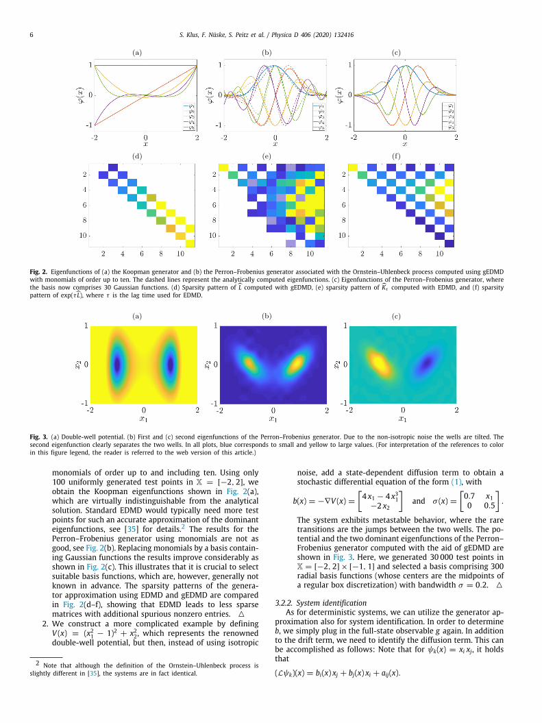
Fig. 2. Eigenfunctions of (a) the Koopman generator and (b) the Perron–Frobenius generator associated with the Ornstein–Uhlenbeck process computed using gEDMDwith monomials of order up to ten. The dashed lines represent the analytically computed eigenfunctions. (c) Eigenfunctions of the Perron–Frobenius generator, wherethe basis now comprises 30 Gaussian functions. (d) Sparsity pattern of L computed with gEDMD, (e) sparsity pattern of Kτ computed with EDMD, and (f) sparsitypattern of exp(τ L), where τ is the lag time used for EDMD.

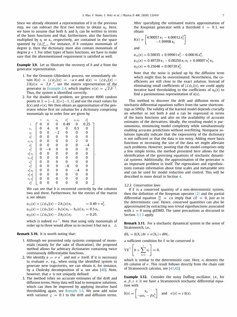
Fig. 3. (a) Double-well potential. (b) First and (c) second eigenfunctions of the Perron–Frobenius generator. Due to the non-isotropic noise the wells are tilted. Thesecond eigenfunction clearly separates the two wells. In all plots, blue corresponds to small and yellow to large values. (For interpretation of the references to colorin this figure legend, the reader is referred to the web version of this article.)

monomials of order up to and including ten. Using only100 uniformly generated test points in X = [−2, 2], weobtain the Koopman eigenfunctions shown in Fig. 2(a),which are virtually indistinguishable from the analyticalsolution. Standard EDMD would typically need more testpoints for such an accurate approximation of the dominanteigenfunctions, see [35] for details.2 The results for thePerron–Frobenius generator using monomials are not asgood, see Fig. 2(b). Replacing monomials by a basis contain-ing Gaussian functions the results improve considerably asshown in Fig. 2(c). This illustrates that it is crucial to selectsuitable basis functions, which are, however, generally notknown in advance. The sparsity patterns of the genera-tor approximation using EDMD and gEDMD are comparedin Fig. 2(d–f), showing that EDMD leads to less sparsematrices with additional spurious nonzero entries. △

2. We construct a more complicated example by definingV (x) = (x21 − 1)2 + x22, which represents the renowneddouble-well potential, but then, instead of using isotropic

2 Note that although the definition of the Ornstein–Uhlenbeck process isslightly different in [35], the systems are in fact identical.

noise, add a state-dependent diffusion term to obtain astochastic differential equation of the form (1), with

b(x) = −∇V (x) =

[4 x1 − 4 x31

−2 x2

]and σ (x) =

[0.7 x10 0.5

].

The system exhibits metastable behavior, where the raretransitions are the jumps between the two wells. The po-tential and the two dominant eigenfunctions of the Perron–Frobenius generator computed with the aid of gEDMD areshown in Fig. 3. Here, we generated 30 000 test points inX = [−2, 2] × [−1, 1] and selected a basis comprising 300radial basis functions (whose centers are the midpoints ofa regular box discretization) with bandwidth σ = 0.2. △

3.2.2. System identificationAs for deterministic systems, we can utilize the generator ap-

proximation also for system identification. In order to determineb, we simply plug in the full-state observable g again. In additionto the drift term, we need to identify the diffusion term. This canbe accomplished as follows: Note that for ψk(x) = xi xj, it holdsthat

(Lψk)(x) = bi(x) xj + bj(x) xi + aij(x).

S. Klus, F. Nüske, S. Peitz et al. / Physica D 406 (2020) 132416 7

Since we already obtained a representation of b in the previousstep, we can subtract the first two terms to obtain aij. Here,we have to assume that both bi and bj can be written in termsof the basis functions and that, furthermore, also the functionsmultiplied by xj or xi, respectively, are contained in the spacespanned by {ψi}

ni=1. For instance, if b contains monomials of

degree p, then the dictionary must also contain monomials ofdegree p+1. For other types of basis functions, we have to makesure that the aforementioned requirement is satisfied as well.

Example 3.9. Let us illustrate the recovery of b and a from thegenerator representation.

1. For the Ornstein–Uhlenbeck process, we immediately ob-tain b(x) = (Lψ2)(x) = −α x and a(x) = (Lψ3)(x) −

2 b(x) x = 2β−1, see the matrix representation of thegenerator in Example 2.4, which implies σ (x) =

√2β−1.

Thus, the system is identified correctly.2. For the double-well problem, we generate 8000 random

points in X = [−2, 2]×[−1, 1] and use the exact values forb(x) and σ (x). We then obtain an approximation of the gen-erator whose first six columns for a dictionary comprisingmonomials up to order four are given by

⎡⎢⎢⎢⎢⎢⎢⎢⎢⎢⎢⎢⎢⎢⎢⎢⎢⎢⎢⎢⎢⎢⎣

1 x1 x2 x21 x1 x2 x221 0 0 0 0.49 0 0.25x1 0 4 0 0 0.5 0x2 0 0 −2 0 0 0x21 0 0 0 9 0 0

x1 x2 0 0 0 0 2 0x22 0 0 0 0 0 −4x31 0 −4 0 0 0 0

x21 x2 0 0 0 0 0 0x1 x22 0 0 0 0 0 0x32 0 0 0 0 0 0x41 0 0 0 −8 0 0

x31 x2 0 0 0 0 −4 0x21 x22 0 0 0 0 0 0x1 x32 0 0 0 0 0 0x42 0 0 0 0 0 0

⎤⎥⎥⎥⎥⎥⎥⎥⎥⎥⎥⎥⎥⎥⎥⎥⎥⎥⎥⎥⎥⎥⎦

.

We can see that b is recovered correctly by the columnstwo and three. Furthermore, for the entries of the matrixa, we obtain

a11(x) = (Lψ4)(x) − 2 b1(x) x1 = 0.49 + x21,a12(x) = (Lψ5)(x) − b1(x) x2 − b2(x) x1 = 0.5 x1,a22(x) = (Lψ6)(x) − 2 b2(x) x2 = 0.25,

which is indeed σσ⊤. Note that using only monomials oforder up to three would allow us to recover b but not a. △

Remark 3.10. It is worth noting that:

1. Although we presented only systems composed of mono-mials (mainly for the sake of illustration), the proposedmethod allows for arbitrary dictionaries containing twicecontinuously differentiable functions.

2. We identify a = σ σ⊤ and not σ itself. If it is necessaryto evaluate σ , e.g., when using the identified system togenerate new trajectories, we can obtain it, for instance,by a Cholesky decomposition of a, see also [40]. Note,however, that σ is not uniquely defined.

3. The method relies on accurate estimates of the drift anddiffusion terms. Noisy data will lead to nonsparse solutions,which can then be improved by applying iterative hardthresholding again, see Remark 3.4. We now add noisewith variance ς = 0.1 to the drift and diffusion terms.

After sparsifying the estimated matrix approximation ofthe Koopman generator with a threshold δ = 0.1, weobtain

b(x) =

[4.00057 x1 − 4.00012 x31

−1.99998 x2

]and

a11(x) = 0.50035 + 0.99901 x21 − 0.00016 x41,

a12(x) = 0.49729 x1 − 0.00250 x1 x2 + 0.00097 x31 x2,

a22(x) = 0.25648 + 0.00720 x22.

Note that the noise is picked up by the diffusion termwhich might thus be overestimated. Nevertheless, the co-efficients are still close to the exact solution. Instead ofeliminating small coefficients of (Lψk)(x), we could applyiterative hard thresholding to the coefficients of aij(x) tofind a parsimonious representation of a(x).

This method to discover the drift and diffusion terms ofstochastic differential equations suffers from the same shortcom-ings as SINDy: The validity of the learned model depends cruciallyon whether or not both b and a can be expressed in termsof the basis functions and also on the availability of accurateestimates of the derivatives. Ideally, the resulting model is par-simonious, minimizing model complexity while simultaneouslyenabling accurate predictions without overfitting. Nonsparse so-lutions typically indicate that the expressivity of the dictionaryis not sufficient or that the data is too noisy. Adding more basisfunctions or increasing the size of the data set might alleviatesuch problems. However, positing that the model comprises onlya few simple terms, the method presented here allows for theidentification of the governing equations of stochastic dynami-cal systems. Additionally, the approximation of the generator isan important problem in itself. The eigenvalues and eigenfunc-tions contain information about time scales and metastable setsand can be used for model reduction and control. This will bedescribed in more detail in Section 4.

3.2.3. Conservation lawsIf E is a conserved quantity of a non-deterministic system,

then the definition of the Koopman operator (2) and the partialdifferential equation ∂u

∂t = Lu imply that LE = 0, just as inthe deterministic case. Hence, conserved quantities can also beapproximated by extracting non-trivial eigenfunctions associatedwith λ = 0 using gEDMD. The same precautions as discussed inSection 3.1.3 apply.

Remark 3.11. For a stochastic dynamical system in the sense ofStratonovich, i.e.,

dXt = b(Xt ) dt + σ (Xt ) ◦ dWt ,

a sufficient condition for E to be conserved is

∇E⊤

[b +

s∑i=1

σi

]= 0,

which is similar to the deterministic case. Here, σi denotes theith column of σ . This result follows directly from the chain ruleof Stratonovich calculus, see [41,42].

Example 3.12. Consider the noisy Duffing oscillator, i.e., forα, β, ε ∈ R we have a Stratonovich stochastic differential equa-tion with

b(x) =

[x2

−αx1 − βx31

]and σ (x) = ε b(x).

8 S. Klus, F. Nüske, S. Peitz et al. / Physica D 406 (2020) 132416

To apply gEDMD, we convert it to an Itô stochastic differen-tial equation using the drift correction formula to correct thenoise-induced drift, which is defined componentwise as

ci(x) =

d∑j=1

s∑k=1

∂σik

∂xj(x) σjk(x), i = 1, . . . , d,

see [43]. We obtain the Itô stochastic differential equation

dXt =(b(Xt ) +

12 c(Xt )

)dt + σ (Xt ) dWt with

c(x) = ε2[

b2(x)(−α − 3βx21

)b1(x)

].

Setting α = −1.1, β = 1.1, ε = 0.05, choosing a dictionary thatcontains monomials, and applying gEDMD, the multiplicity of theeigenvalue λ = 0 is two and we obtain a conserved quantity ofthe form

E(x) ≈α2 x

21 +

β

4 x41 +

12x

22 + c,

where c ∈ R is an arbitrary constant. △

3.3. Relationships with other methods

We will now point out similarities and differences betweenthe methods presented above and other well-known approachesfor systems identification and generator approximation.

3.3.1. SINDySINDy [5] was designed to learn ordinary differential equa-

tions from simulation or measurement data. Just like gEDMD, itrequires a set of states and the corresponding time derivatives.Defining X = [x1, x2, . . . , xm], SINDy minimizes the cost function∥X − MSΨX∥F , i.e., MS = XΨ +

X . Here, we omit the sparsificationconstraints, which can be added in the same way to gEDMDas described above. Recall that we assume that the full-stateobservable is given by g(x) = B⊤ψ(x). SINDy can thus be seenas a special case of gEDMD since

x = B⊤ψ(x) ≈ B⊤Mψ(x) = B⊤ΨX X

Ψ +

X ψ(x) = XΨ +

XMS

ψ(x) = MS ψ(x).

3.3.2. Koopman lifting techniqueThe Koopman lifting technique [22,23] uses the infinitesimal

generator L for system identification. While tailored mainly toordinary differential equations, extensions to stochastic differen-tial equations with isotropic noise are also considered. First, theKoopman operator for a fixed lag time τ is estimated from trajec-tory data with the aid of standard EDMD. Then an approximationof the generator is obtained by taking the matrix logarithm, i.e.,

L =1τlog Kτ ,

where Kτ is the matrix representation of the Koopman operatorwith respect to the chosen basis ψ (and lag time τ ). The laststep is to estimate the governing equations in the same wayas illustrated in Example 3.3 for gEDMD. The Koopman liftingtechnique does not require the time-derivatives of the states orthe partial derivatives of the basis functions, but only pairs oftime-lagged data. However, the non-uniqueness of the matrixlogarithm can cause problems and a sufficiently small samplingtime τ is needed to ensure that the (possibly complex) eigen-values lie in the strip {z ∈ C : |ℑ(z)| < π}, where ℑ denotes theimaginary part. Roughly speaking, only an infinite sampling rateallows us to capture the entire spectrum of frequencies [23]. Ourapproach generalizes to arbitrary systems of the form (1), but theestimation of the diffusion term can be carried over to the liftingtechnique as well. This could be a valuable alternative, e.g., when

only trajectory data is available. If the exact derivatives for thetraining data are known, then gEDMD is in general more accuratethan the lifting approach. If, on the other hand, the derivativesfor gEDMD have to be approximated from trajectory data, thenthe accuracy depends on the order of the finite-difference ap-proximation and the step size, while the accuracy of the liftingapproach depends on the lag time and the matrix logarithmimplementation.

3.3.3. KRONICKRONIC [19,20], which stands for Koopman reduced order non-

linear identification and control, is a data-driven method fordiscovering Koopman eigenfunctions, which are then used forcontrol and the detection of conservation laws. The approachis based on SINDy and assumes that an eigenvalue is known apriori (or simultaneously learns the eigenvalue and correspond-ing eigenfunction). In our notation, the resulting problem can bewritten as(λℓΨ

⊤

X − Ψ ⊤

X

)ξℓ = 0,

which, multiplying from the left by ΨX and assuming that ΨXΨ⊤

Xis regular, becomes the gEDMD eigenvalue problem. This operatorformulation is briefly mentioned in [19] as well. Thus, for deter-ministic systems, despite their different derivations, gEDMD andKRONIC are strongly related.

4. Further applications

In addition to identifying fast and slow modes, governingequations, or conservation laws, the Koopman generator has fur-ther applications that we will briefly demonstrate.

4.1. Coarse-grained dynamics and gEDMD

4.1.1. Galerkin approximationIn what follows, we describe how models of the Koopman

generator can be used to identify reduced order models of a(possibly high-dimensional) stochastic dynamical system. To getstarted, we recapitulate the model reduction formalism intro-duced by [40,44]. Assume the stochastic process given by (1)possesses a unique invariant density µ, and let ξ :Rd

→ Rp be acoarse-graining function which maps Rd to a lower-dimensionalspace Rp. The coarse-graining map induces a reduced probabilitymeasure with density ν on Rp. Consider the space L2ν of square-integrable functions of the reduced variables z. In fact, L2ν is aninfinite-dimensional subspace of L2µ, if each function f ∈ L2ν isidentified with the function f ◦ ξ ∈ L2µ. Let P be the orthogonalprojection onto L2ν . Define a coarse-grained generator as

Lξ = PLP. (6)

Given suitable assumptions on the original process (1), Lξ is againthe infinitesimal generator of a stochastic dynamics on Rp, withinvariant density ν and effective drift and diffusion coefficientbξ , aξ [40,44].

First, we show that for a basis set of functions defined onlyon Rp, gEDMD converges to a Galerkin approximation of thecoarse-grained generator Lξ :

Proposition 4.1. Let V = span{ψk}nk=1 be a subspace of L2ν . Then

gEDMD applied to the functions ψk = ψk ◦ ξ converges to theGalerkin projection of Lξ onto V. Here, (5) needs to be updated by

dψk(x) = b(x)∇x ξ (x)∇zψ⊤

k (ξ (x)) +12(a(x) : Hξ (x))∇zψ

⊤

k (ξ (x))

+12∇

2zψk(ξ (x)) :

[∇ξ (x)⊤a(x)∇ξ (x)

],

S. Klus, F. Nüske, S. Peitz et al. / Physica D 406 (2020) 132416 9

where ∇x ξ ∈ Rd×p is the Jacobian of ξ , and Hξ ∈ Rd×d×p

is the tensor of Hessian matrices for each component of ξ . TheFrobenius inner product between a and Hξ is applied to the first twodimensions of Hξ .

Proof. The expression for dψk(x) follows from the chain rule. Itwas already shown in [40] that⟨

ψi, ψj⟩ν

=⟨ψi ◦ ξ, ψj ◦ ξ

⟩µ,⟨

Lξψi, ψj⟩ν

=⟨L(ψi ◦ ξ ), ψj ◦ ξ

⟩µ.

Thus, Proposition 3.5 implies that

Aij →⟨Lψi, ψj

⟩µ

=⟨Lξψi, ψj

⟩ν,

Gij →⟨ψi, ψj

⟩µ

=⟨ψi, ψj

⟩ν. □

In summary, data of the original process, sampling the dis-tribution µ, can be used to learn a matrix representation ofthe coarse-grained generator (6). This matrix approximation canthen be used to perform system identification, simulation, andcontrol of the coarse-grained system the same way as describedin Section 3.2.

4.1.2. Separate identificationFor a reversible stochastic differential equation (1), we present

an alternative approach to identify the parameters of the corre-sponding coarse-grained system. The method is related to spec-tral matching as introduced in [45]. The authors of [40] haveshown that reversibility of the full process implies the dynamicsgenerated by (6) are also reversible. Recalling that reversibledynamics are characterized by a scalar potential and the diffu-sion field, the basic idea is simply to estimate these two termsseparately. The resulting framework, which we will call sepa-rate identification, consists of four steps, which are only partiallydependent on each other:

Force matching. The scalar potential F ξ of the coarse-graineddynamics can be estimated by an established technique calledforce matching [46,47]. It is based on the fact that the gradientof F ξ solves the following minimization problem [48]:

∇zF ξ = argming∈(L2ν )p

∫Rd

∥g(ξ (x)) − f ξlmf (x)∥2 dµ(x), (7)

f ξlmf = −∇xF · Gξ + ∇x · Gξ , (8)

Gξ = ∇xξ[(∇xξ )T∇xξ

]−1, (9)

where the minimization is over all square-integrable vector fieldsg of the reduced variables z, and the divergence is applied sepa-rately to each column of Gξ in (8). The vector field f ξlmf is calledlocal mean force, while F is the scalar potential of the full process.

Application of gEDMD. The second step consists of applyinggEDMD to estimate a finite-dimensional model of the coarse-grained generator Lξ as described in Section 4.1.1, using a basis offunctions {ψi}

ni=1 defined on the reduced space Rp. In particular,

we obtain an estimate of the Galerkin matrix

Aij =⟨Lξψi, ψj

⟩ν.

Learning the diffusion field. As already discussed in Remark 3.7,matrix elements of the reduced generator are given by⟨Lξψi, ψj

⟩ν

= −12

∫∇zψi aξ ∇zψj dν. (10)

It follows that the effective diffusion can be learned by matchingit to the generator matrix A via (10). Let aξ (θ ) be a paramet-ric model for the effective diffusion. Then the optimal set of

parameters can be found by minimizing the Frobenius norm error

E(θ ) = ∥A − A(θ )∥2F , (11)

A(θ )ij = −12

∫∇zψi aξ (θ )∇zψj dν. (12)

Determination of the drift. Using the relationship between driftand diffusion of a reversible system, inserting estimates for F ξand aξ into (13) completes the definition of the reduced model

bξ = −12aξ ∇F ξ +

12∇ · aξ . (13)

The above formulation seems advantageous compared to thedirect system identification described in Section 3.2.2 for severalreasons:

• Separate basis sets can be used to calculate the Galerkinmatrix, the potential, and the diffusion. Specifically, con-straints on each of these (such as positive definiteness of thediffusion) can be incorporated into each basis individually.Moreover, learning of the potential and the diffusion canalso be accomplished using nonlinear models.

• The coordinate functions zi and zi zj, as well as the productsof the coordinate functions with the effective drift, are nolonger required to be contained in the basis set.

• Both force matching and (11) are regression problems, al-lowing for the use of model validation techniques like cross-validation.

• The dynamics obtained by combining the learned potentialand diffusion via (13) are automatically reversible.

• By diagonalizing the generator matrix corresponding to A(θ )above, the spectrum of the learned dynamics can be calcu-lated directly and compared to the spectrum of the genera-tor matrix corresponding to A, providing a further means ofmodel validation.

On the other hand, the direct system identification is moregeneral since the reconstruction via the local mean force may failto yield good approximations of the effective drift in cases wheresome parts of the dynamics orthogonal to the low-dimensionalmanifold defined by the reaction coordinate are slow.

4.1.3. Example 1: Lemon-slice potentialWe consider overdamped Langevin dynamics (see Remark 2.2)

at inverse temperature β = 1 in the following two-dimensionalpotential V , expressed in polar coordinates:

V (r, ϕ) = cos(kϕ) + sec(0.5ϕ) + 10(r − 1)2 +1r.

For k = 4, a contour of the potential is shown in Fig. 4(a). Becauseof the two singular terms, the system’s state space does notinclude the set {(x1, x2) : x1 ≤ 0, x2 = 0}, enabling us to map thetwo-dimensional state space to polar coordinates unambiguously.

The polar angle ϕ is a suitable reaction coordinate, so wechoose ξ (x1, x2) = ϕ(x1, x2). Due to the simplicity of the system,all relevant quantities can be calculated analytically. Using thefull-state partition function Z and two numerical constants C1, C2,see [49], the invariant distribution, the effective drift and theeffective diffusion along ϕ are given by

ν(ϕ) =C2

Zexp (− [cos(kϕ) + sec(0.5ϕ)]) ,

bϕ(ϕ) =C1

C2[k sin(kϕ) − 0.5 tan(0.5ϕ) sec(0.5ϕ)] ,

aϕ(ϕ) =2 C1

C2.

10 S. Klus, F. Nüske, S. Peitz et al. / Physica D 406 (2020) 132416

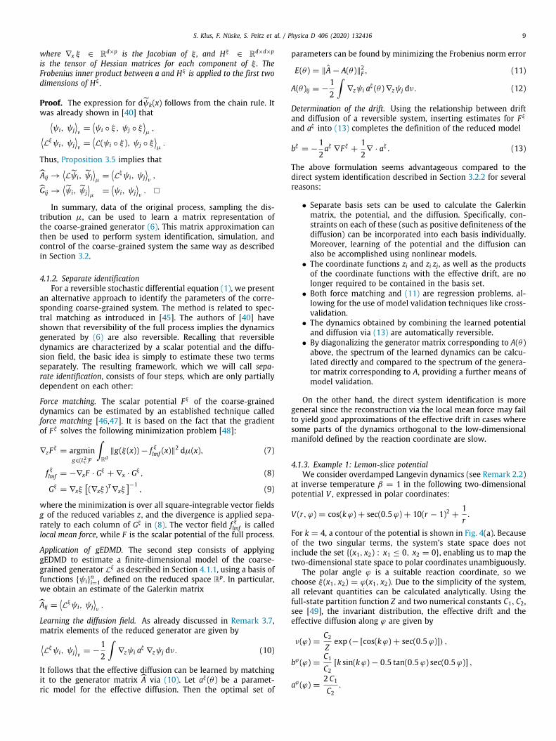
Fig. 4. Application of gEDMD with 21 Legendre polynomials to one-dimensional coarse-graining of the two-dimensional lemon-slice potential. (a) Visualization ofthe potential. (b) Estimates of the effective drift along the polar angle ϕ obtained directly from the generator matrix (blue), and by combining the solutions of(11) and (7) via (13) (red). The analytical reference is shown in yellow. (c) Estimates of the effective diffusion along the polar angle ϕ obtained directly from thegenerator matrix (blue), and by learning the diffusion via (11) using a Gaussian basis set (red), compared to the analytical reference in yellow. (d) Estimates of thethree slowest implied time scales using a Markov state model (yellow), diagonalization of the generator matrix (blue), and diagonalization of the generator matrixcorresponding to the optimal diffusion (red). (For interpretation of the references to color in this figure legend, the reader is referred to the web version of thisarticle.)

We apply coarse-grained gEDMD with a basis set of Legendrepolynomials up to degree 20, scaled to fit the domain [−π, π].In this example and the next, we use exact expressions for thedrift and diffusion coefficient, as the parameters of the full sys-tem are usually known in the context of model reduction. Fromthe generator matrix, we obtain estimates of the effective driftand diffusion as described in Section 3.2.2. Moreover, we alsoapply separate identification to learn the scalar potential and thediffusion. To this end, we use a basis set of periodic Gaussianfunctions centered at equidistant points between ϕ = −2.8 andϕ = 2.8. The bandwidth of these Gaussians is determined bycross-validation, and is found to be 0.1 for force matching and2.0 for the diffusion. We also enforce positivity of the diffusionby applying positivity constraints to the regression problem (11).We see in Fig. 4(b) and (c) that both methods provide accuraterepresentations of the effective parameters. However, the diffu-sion estimated from (11) is virtually indistinguishable from theanalytical solution, while the representation obtained from thepolynomial basis is more oscillatory.

We also verify that gEDMD correctly captures the slow dy-namics in this example. We diagonalize the generator matrixobtained from the polynomial basis, and compute the first threeimplied time scales by taking reciprocals of the first three non-trivial eigenvalues (leaving out the zero eigenvalue). We comparethese time scales to those extracted from a Markov state model(MSM) [50] inferred directly from the data. We find in Fig. 4(d)

that the time scales are in very good agreement. As describedabove, we also use the generator matrix corresponding to theoptimal A(θ ) to estimate the first three implied time scales, andfind them to match almost perfectly as well.

4.1.4. Example 2: Alanine dipeptideAs a more complex example, we derive a coarse-grained

model from molecular dynamics simulations of alanine dipeptide,which has been used as a test case in numerous previous studies.The data set is the same as in reference [51] and comprises onemillion snapshots of Langevin dynamics saved every 1 ps. As iswell-known, the positional component of Langevin dynamics be-haves approximately like an overdamped process, see Remark 2.2,up to a re-scaling of time. Hence, we apply gEDMD assuming theoriginal process is overdamped, and we extract this effective unitof time by comparing the first two implied time scales obtainedfrom gEDMD and from a reference Markov state model.

The slowest dynamics of alanine dipeptide are captured bya single internal molecular coordinate, called φ-dihedral angle,which we choose to be the coarse-graining coordinate. Fig. 5(a)shows the empirical coarse-grained energy Fφ , and an approx-imation obtained by applying force matching. The basis set forforce matching consists of 57 periodic Gaussians of bandwidth1.2, centered at equidistant points between −2.8 and 2.8. Theslowest dynamical process corresponds to the transition acrossthe highest barrier in this energy landscape.

S. Klus, F. Nüske, S. Peitz et al. / Physica D 406 (2020) 132416 11

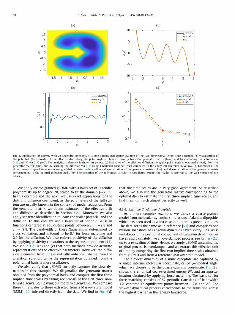
Fig. 5. Coarse-grained gEDMD along the φ-angle coordinate of alanine dipeptide, using a basis set of 26 Legendre polynomials (a) Effective energy Fφ , as estimatedby histogramming the molecular dynamics simulation data (black), and by applying force matching with a Gaussian basis set (blue). (b) Estimates of the effectivedrift obtained directly from the generator matrix (blue), and by combining the solutions of (11) and (7) via (13) (red). (c) Estimates of the effective diffusion obtaineddirectly from the generator matrix (blue), and by learning the diffusion via (11) using a Gaussian basis set (red). (d) Estimates of the two slowest implied timescales using a Markov state model (yellow), diagonalization of the generator matrix (blue), and diagonalization of the generator matrix corresponding to the optimaldiffusion (red). (For interpretation of the references to color in this figure legend, the reader is referred to the web version of this article.)

We apply gEDMD with the first 26 Legendre polynomialsscaled to fit the domain [−2.7, 2.7]. From the generator matrix,we extract the effective drift and diffusion, which are depicted byblue lines in Fig. 5(b) and (c). As a comparison, we also computean estimate of the effective diffusion by minimization of (11),including positivity constraints, with a set of 29 Gaussians ofbandwidth 0.8, where the optimal bandwidth was determined bycross-validation. The resulting estimate of the diffusion is far lessoscillatory than the direct estimate using the generator matrix,while the corresponding drift obtained from (13) is similar to thedirect estimate.

Finally, we verify that gEDMD accurately reproduces the spec-tral properties of the original dynamics. As we can see in Fig. 5(d),after re-scaling the first two time scales provided by gEDMD bythe effective time unit described above, they agree well with theresults of an MSM analysis. The same is true for the time scalescalculated based on the generator matrix corresponding to theoptimal diffusion obtained by solving (11).

4.2. Control

The predictive capabilities of the Koopman operator have alsoraised interest in the control community, where the aim is to de-termine a system input u such that the non-autonomous controlsystem x = b(x, u) behaves in a desired way, which results in the

following control problem:

minu∈L2([t0,te],R)

J(x, u) = minu∈L2([t0,te],R)

∫ te

t0

x(t) − xref(t)22 + α∥u(t)∥2

2 dt

s.t. x(t) = b(x(t), u(t)),

x(t0) = x0.

(14)

In this formulation, the goal is to track a desired state over thecontrol horizon [t0, te], and α ∈ R>0 is a small number penalizingthe control cost. In order to achieve a feedback behavior, problem(14) is embedded into a model predictive control (MPC) [52]scheme, where it has to be solved repeatedly over a relativelyshort horizon while the system (the plant) is running at the sametime. The first part [t0, t0 + h] of the optimal control u is thenapplied to the plant, and (14) has to be solved again on a shiftedhorizon [t0 + h, te + h].

Since the real-time requirements in MPC are often very hard tosatisfy, a promising approach is to replace the system dynamicsby a surrogate model, and one possibility is to use the Koopmanoperator or its generator for prediction. Introducing the variablez = ψ(f (x)), we obtain a linear system via the approximation Lof the generator:

z(t) ≈ Lz(t).

However, as we see above, the Koopman operator is only definedfor autonomous systems. Hence, a transformation has to be used

12 S. Klus, F. Nüske, S. Peitz et al. / Physica D 406 (2020) 132416

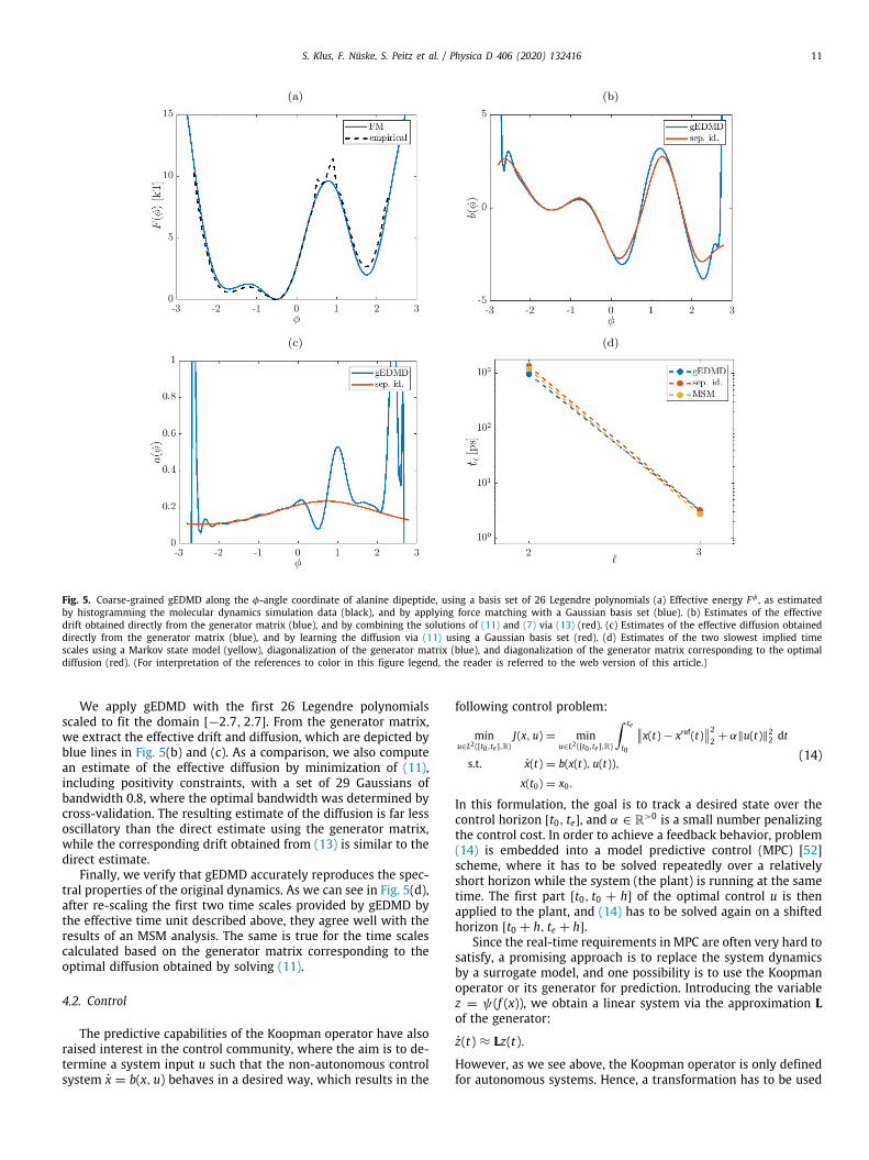
Fig. 6. Control of the Burgers equation using the Koopman generator and switching control. (a) The shape function used for the distributed control term. (b) Theoptimal state (colored) and the reference trajectories (black) for h = 0.05. (c) The optimal switching sequence as a function of the time step h. (d) The tracking erroras a function of the time step h. (For interpretation of the references to color in this figure legend, the reader is referred to the web version of this article.)

(the exception being control-affine systems, where only the au-tonomous part needs to be modeled). In [53], the control systemwas autonomized by introducing an augmented state x = (x, u)⊤,and DMD was performed on the augmented system. The sameapproach was also used in combination with MPC in [54]. Thisstate augmentation significantly increases the data requirements(all combinations of states and control inputs should be covered),such that an alternative transformation was proposed in [55,56]by restricting u(t) to a finite set of inputs {u1, . . . , unc }. This way,the control system can be replaced by a finite set of autonomoussystems bui (x) = b(x, ui) for which the corresponding generators{Lu1 , . . . , Lunc } can be approximated. The control task is thus todetermine the optimal right-hand side in each time step insteadof computing a continuous input u:

minu∈L2([t0,te],{u1,...,unc })

∫ te

t0

z(t) − zref(t)22 + α∥u(t)∥2

2 dt

s.t. z(t) = Lu(t)z(t),z(t0) = ψ(f (x0)).

(15)

Note that the quantization (i.e., the switching control) is encodedin the function space the control u lives in. For a more detaileddescription, the reader is referred to [55].

Regardless of the approach, a drawback of Koopman operatorbased surrogate models is that the control freedom is limited bythe finite lag time. While larger lag times are often beneficial forthe approximation of the dynamics, this is counterproductive forcontrol, as the control frequency is strongly limited. This issue isovercome by the generator approach (15) since we can choosearbitrary time steps here, and results on mixed integer optimalcontrol problems (see, e.g., [57]) suggest that fast switches allowfor solutions of any desired accuracy. Moreover, the continuous-time generator model is much better suited for switching timeoptimization approaches. Therein, the combinatorial problem of

selecting the optimal right-hand side is replaced by a continuousoptimization problem for the time instances τj at which theright-hand side is switched from the input ui to ui+1:

minτ∈Rp

∫ te

t0

z(t) − zref(t)22 + α∥u(t)∥2

2 dt

s.t. z(t) = Luiz(t), for t ∈ [τj−1, τj),t0 = τ0 ≤ τ1 ≤ · · · ≤ τp ≤ te,i = 1 + j mod nc,

z(t0) = ψ(f (x0)).

(16)

By fixing the number p of switches, this reformulation of (15) isnow a continuous, finite-dimensional optimization problem forthe switching times with a given switching sequence (cf. [58] fordetails), and both open and closed-loop control schemes (usingMPC in the latter case) can be constructed.

Problem (16) was also used in combination with the Koopmanoperator in [55], but the discrete-time system prohibits arbitraryswitching points which results in a reduced performance. Usingthe generator solves this problem and additionally, there evenexist efficient second-order methods for this problem class [59].

In what follows, we present examples for the two extensionsfor MPC based on the Koopman generator. For the deterministiccase, we use the 1D viscous Burgers equation with varying lagtimes in an MPC framework (Problem (15)) and for the non-deterministic case, we control the expected value of an Ornstein–Uhlenbeck process using both MPC (Problem (15)) and open loopswitching time control (Problem (16)).

4.2.1. Partial differential equationsConsider the 1D Burgers equation with distributed control

y(t, x) − ν∆y(t, x) + y(t, x)∇y(t, x) = u(t)χ (x).

S. Klus, F. Nüske, S. Peitz et al. / Physica D 406 (2020) 132416 13

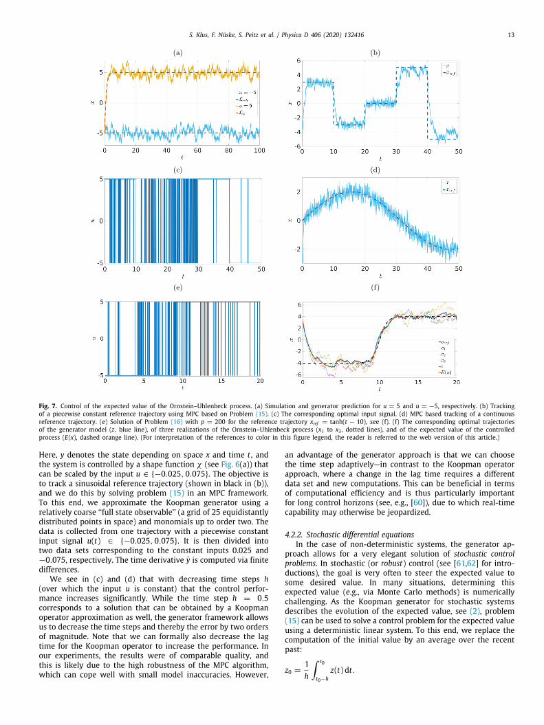
Fig. 7. Control of the expected value of the Ornstein–Uhlenbeck process. (a) Simulation and generator prediction for u = 5 and u = −5, respectively. (b) Trackingof a piecewise constant reference trajectory using MPC based on Problem (15). (c) The corresponding optimal input signal. (d) MPC based tracking of a continuousreference trajectory. (e) Solution of Problem (16) with p = 200 for the reference trajectory xref = tanh(t − 10), see (f). (f) The corresponding optimal trajectoriesof the generator model (z, blue line), of three realizations of the Ornstein–Uhlenbeck process (x1 to x3 , dotted lines), and of the expected value of the controlledprocess (E(x), dashed orange line). (For interpretation of the references to color in this figure legend, the reader is referred to the web version of this article.)

Here, y denotes the state depending on space x and time t , andthe system is controlled by a shape function χ (see Fig. 6(a)) thatcan be scaled by the input u ∈ {−0.025, 0.075}. The objective isto track a sinusoidal reference trajectory (shown in black in (b)),and we do this by solving problem (15) in an MPC framework.To this end, we approximate the Koopman generator using arelatively coarse ‘‘full state observable’’ (a grid of 25 equidistantlydistributed points in space) and monomials up to order two. Thedata is collected from one trajectory with a piecewise constantinput signal u(t) ∈ {−0.025, 0.075}. It is then divided intotwo data sets corresponding to the constant inputs 0.025 and−0.075, respectively. The time derivative y is computed via finitedifferences.

We see in (c) and (d) that with decreasing time steps h(over which the input u is constant) that the control perfor-mance increases significantly. While the time step h = 0.5corresponds to a solution that can be obtained by a Koopmanoperator approximation as well, the generator framework allowsus to decrease the time steps and thereby the error by two ordersof magnitude. Note that we can formally also decrease the lagtime for the Koopman operator to increase the performance. Inour experiments, the results were of comparable quality, andthis is likely due to the high robustness of the MPC algorithm,which can cope well with small model inaccuracies. However,

an advantage of the generator approach is that we can choosethe time step adaptively—in contrast to the Koopman operatorapproach, where a change in the lag time requires a differentdata set and new computations. This can be beneficial in termsof computational efficiency and is thus particularly importantfor long control horizons (see, e.g., [60]), due to which real-timecapability may otherwise be jeopardized.

4.2.2. Stochastic differential equationsIn the case of non-deterministic systems, the generator ap-

proach allows for a very elegant solution of stochastic controlproblems. In stochastic (or robust) control (see [61,62] for intro-ductions), the goal is very often to steer the expected value tosome desired value. In many situations, determining thisexpected value (e.g., via Monte Carlo methods) is numericallychallenging. As the Koopman generator for stochastic systemsdescribes the evolution of the expected value, see (2), problem(15) can be used to solve a control problem for the expected valueusing a deterministic linear system. To this end, we replace thecomputation of the initial value by an average over the recentpast:

z0 =1h

∫ t0

t0−hz(t) dt.

14 S. Klus, F. Nüske, S. Peitz et al. / Physica D 406 (2020) 132416

We again consider the Ornstein–Uhlenbeck process fromExample 2.3, with the only difference that we now add a controlinput:

dXt = −α (Xt − u) dt +

√2β−1 dWt ,

with α = 1 and β = 2. We compute two generator approxima-tions corresponding to u = −5 and u = 5 using monomials upto order 12. Fig. 7(a) shows the trajectories of the two systemsand the predictions using the corresponding generators, and wesee that the expected values are accurately predicted. We seth = 0.05 as a discretization for the control u as well as the lengthof the input that is applied to the plant in each loop. The MPCcontroller based on (15) with the modified initial condition z0yields very good performance, as is shown for a tracking problemwith a piecewise constant reference value in Fig. 7(b). The corre-sponding optimal control is shown in Fig. 7(c), and (d) shows thatcontinuously varying inputs can be approximated equally well.

Finally, we use the switching time reformulation (16) in anopen loop fashion in order to track a tanh profile over 20 s. Theresults are shown in Fig. 7(e) and (f), where the optimal inputwith p = 200 switches is shown in (e) and the corresponding dy-namics are shown in (f). We observe a remarkable performance,as the optimal trajectory of the generator model and the expectedvalue of the controlled Ornstein–Uhlenbeck process (computed asthe mean over 1000 simulations) are almost indistinguishable.

To summarize, the generator approach yields highly efficientcontrol schemes both for open and closed-loop control, as thelinear system for the prediction of the expected value requiresno further sampling of multiple noisy trajectories.

5. Conclusion

We presented an extension of standard EDMD to approximatethe generator of the Koopman or Perron–Frobenius operator fromdata and highlighted several important applications pertainingto model reduction, system identification, and control. We illus-trated that this approach can be used to obtain a decompositioninto eigenvalues, eigenfunctions, and modes and, furthermore,that SINDy emerges as a special case. The proposed methods wereimplemented in Python, the gEDMD code and some of the aboveexamples are available at https://github.com/sklus/d3s/.

Open questions include the convergence of gEDMD if not onlythe number of data points but also the number of basis functionstends to infinity. It is also unclear which part of the spectrum isapproximated if the generator does not possess a pure point spec-trum. Furthermore, is it possible to learn coarse-grained dynamicsby only considering the dominant terms of the decompositionof the system’s equations into eigenvalues, eigenfunctions, andmodes (cf. Example 3.3 and also [45])? Another interesting ap-plication of gEDMD would be to compute committor functionsor hitting times. Extensions to non-autonomous systems will beconsidered in future work.

CRediT authorship contribution statement

Stefan Klus: Conceptualization, Methodology, Software,Investigation. Feliks Nüske: Conceptualization, Methodology,Software, Investigation. Sebastian Peitz: Conceptualization, Me-thodology, Software, Investigation. Jan-Hendrik Niemann:Methodology, Software, Investigation. Cecilia Clementi: Concep-tualization. Christof Schütte: Conceptualization.

Acknowledgments

S. K., J. N., and C. S were funded by Deutsche Forschungsge-meinschaft (DFG), Germany through grant CRC 1114 (Scaling Cas-cades in Complex Systems, project ID: 235221301) and through

Germany’s Excellence Strategy (MATH+: The Berlin MathematicsResearch Center, EXC-2046/1, project ID: 390685689). F. N. waspartially funded by the Rice University Academy of Fellows (USA).F. N. and C. C. were supported by the National Science Foundation,USA (CHE-1265929, CHE-1738990, CHE-1900374, PHY-1427654)and the Welch Foundation, USA (C-1570). C. C. also acknowl-edges funding from the Einstein Foundation Berlin (Germany).S. P. acknowledges support by the DFG Priority Programme 1962(Germany).

References

[1] P.J. Schmid, Dynamic mode decomposition of numerical and experi-mental data, J. Fluid Mech. 656 (2010) 5–28, http://dx.doi.org/10.1017/S0022112010001217.

[2] J.H. Tu, C.W. Rowley, D.M. Luchtenburg, S.L. Brunton, J.N. Kutz, On dynamicmode decomposition: Theory and applications, J. Comput. Dyn. 1 (2) (2014)http://dx.doi.org/10.3934/jcd.2014.1.391.

[3] M.O. Williams, C.W. Rowley, I.G. Kevrekidis, A kernel-based method fordata-driven Koopman spectral analysis, J. Comput. Dyn. 2 (2) (2015)247–265, http://dx.doi.org/10.3934/jcd.2015005.

[4] S. Klus, P. Koltai, C. Schütte, On the numerical approximation of thePerron–Frobenius and Koopman operator, J. Comput. Dyn. 3 (1) (2016)51–79, http://dx.doi.org/10.3934/jcd.2016003.

[5] S.L. Brunton, J.L. Proctor, J.N. Kutz, Discovering governing equations fromdata by sparse identification of nonlinear dynamical systems, Proc. Natl.Acad. Sci. 113 (15) (2016) 3932–3937, http://dx.doi.org/10.1073/pnas.1517384113.

[6] C.R. Schwantes, V.S. Pande, Modeling molecular kinetics with tICA andthe kernel trick, J. Chem. Theory Comput. 11 (2) (2015) 600–608, http://dx.doi.org/10.1021/ct5007357.

[7] S. Klus, I. Schuster, K. Muandet, Eigendecompositions of transfer operatorsin reproducing kernel Hilbert spaces, J. Nonlinear Sci. (2019) http://dx.doi.org/10.1007/s00332-019-09574-z.

[8] S. Klus, P. Gelß, S. Peitz, C. Schütte, Tensor-based dynamic mode de-composition, Nonlinearity 31 (7) (2018) http://dx.doi.org/10.1088/1361-6544/aabc8f.

[9] P. Gelß, S. Klus, J. Eisert, C. Schütte, Multidimensional approximation ofnonlinear dynamical systems, J. Comput. Nonlinear Dyn. 14 (2019) 061006,http://dx.doi.org/10.1115/1.4043148.

[10] C. Chen, A. Surana, A. Bloch, I. Rajapakse, Multilinear time invariantsystems theory, 2019, arXiv e-prints.

[11] Q. Li, F. Dietrich, E.M. Bollt, I.G. Kevrekidis, Extended dynamic modedecomposition with dictionary learning: A data-driven adaptive spectraldecomposition of the Koopman operator, Chaos 27 (10) (2017) 103111,http://dx.doi.org/10.1063/1.4993854.

[12] B. Lusch, J.N. Kutz, S. Brunton, Deep learning for universal linear embed-dings of nonlinear dynamics, Nature Commun. 9 (2017) http://dx.doi.org/10.1038/s41467-018-07210-0.

[13] A. Mardt, L. Pasquali, H. Wu, F. Noé, VAMPnets for deep learning ofmolecular kinetics, Nature Commun. 9 (2018) http://dx.doi.org/10.1038/s41467-017-02388-1.

[14] J.N. Kutz, S.L. Brunton, B.W. Brunton, J.L. Proctor, Dynamic Mode Decom-position: Data-Driven Modeling of Complex Systems, SIAM, Philadelphia,2016.

[15] F. Nüske, B.G. Keller, G. Pérez-Hernández, A.S.J.S. Mey, F. Noé, Variationalapproach to molecular kinetics, J. Chem. Theory Comput. 10 (4) (2014)1739–1752.

[16] B. Koopman, Hamiltonian systems and transformations in Hilbert space,Proc. Natl. Acad. Sci. 17 (5) (1931) 315, http://dx.doi.org/10.1073/pnas.17.5.315.

[17] A. Lasota, M.C. Mackey, Chaos, Fractals, and Noise: Stochastic Aspects ofDynamics, second ed., in: Applied Mathematical Sciences, vol. 97, Springer,New York, 1994.

[18] M. Budišić, R. Mohr, I. Mezić, Applied Koopmanism, Chaos 22 (4) (2012)http://dx.doi.org/10.1063/1.4772195.

[19] E. Kaiser, J.N. Kutz, S.L. Brunton, Data-driven discovery of Koopmaneigenfunctions for control, 2017, ArXiv e-prints.

[20] E. Kaiser, J.N. Kutz, S.L. Brunton, Discovering conservation laws from datafor control, 2018, arXiv e-prints.

[21] L. Boninsegna, F. Nüske, C. Clementi, Sparse learning of stochastic dynam-ical equations, J. Chem. Phys. 148 (24) (2018) 241723, http://dx.doi.org/10.1063/1.5018409.

S. Klus, F. Nüske, S. Peitz et al. / Physica D 406 (2020) 132416 15

[22] A. Mauroy, J. Goncalves, Linear identification of nonlinear systems: Alifting technique based on the Koopman operator, in: 2016 IEEE 55thConference on Decision and Control, CDC, 2016, pp. 6500–6505, http://dx.doi.org/10.1109/CDC.2016.7799269.

[23] A. Mauroy, J. Goncalves, Koopman-based lifting techniques for nonlinearsystems identification, 2017, ArXiv e-prints.

[24] A.N. Riseth, J.P. Taylor-King, Operator fitting for parameter estimation ofstochastic differential equations, 2017, ArXiv e-prints.

[25] D. Giannakis, Data-driven spectral decomposition and forecasting of er-godic dynamical systems, Appl. Comput. Harmon. Anal. 47 (2) (2019)338–396, http://dx.doi.org/10.1016/j.acha.2017.09.001.

[26] G. Froyland, O. Junge, P. Koltai, Estimating long term behavior of flowswithout trajectory integration: The infinitesimal generator approach,SIAM J. Numer. Anal. 51 (1) (2013) 223–247, http://dx.doi.org/10.1137/110819986.

[27] S.L. Brunton, B.W. Brunton, J.L. Proctor, J.N. Kutz, Koopman invariantsubspaces and finite linear representations of nonlinear dynamical systemsfor control, PLoS One 11 (2) (2016) http://dx.doi.org/10.1371/journal.pone.0150171.

[28] B.J. Hollingsworth, Stochastic Differential Equations: A Dynamical SystemsApproach (Ph.D. thesis), Auburn University, 2008.

[29] N. Črnjarić-Žic, S. Maćešić, I. Mezić, Koopman operator spectrum forrandom dynamical systems, 2019, arXiv e-prints.

[30] P. Metzner, Transition Path Theory for Markov Processes: Application toMolecular Dynamics (Ph.D. thesis), Freie Universität Berlin, 2007.

[31] J.R. Baxter, J.S. Rosenthal, Rates of convergence for everywhere-positivemarkov chains, Statist. Probab. Lett. 22 (4) (1995) 333–338, http://dx.doi.org/10.1016/0167-7152(94)00085-M.

[32] G.A. Pavliotis, Stochastic Processes and Applications: Diffusion Pro-cesses, the Fokker–Planck and Langevin Equations, in: Texts in AppliedMathematics, vol. 60, Springer, New York, 2014.

[33] D. Bakry, I. Gentil, M. Ledoux, Analysis and Geometry of Markov DiffusionOperators, Vol. 348, Springer Science & Business Media, 2013.

[34] V. Aboites, Hermite polynomials through linear algebra, Int. J. Pure Appl.Math. 114 (05) (2017) 401–406, http://dx.doi.org/10.12732/ijpam.v114i2.19.

[35] S. Klus, F. Nüske, P. Koltai, H. Wu, I. Kevrekidis, C. Schütte, F. Noé, Data-driven model reduction and transfer operator approximation, J. NonlinearSci. 28 (2018) 985–1010, http://dx.doi.org/10.1007/s00332-017-9437-7.

[36] C. Schütte, M. Sarich, Metastability and Markov State Models in MolecularDynamics: Modeling, Analysis, Algorithmic Approaches, No. 24, in: CourantLecture Notes, American Mathematical Society, 2013.

[37] C. Schütte, M. Sarich, A critical appraisal of Markov state models, Eur.Phys. J. Spec. Top. 224 (12) (2015) 2445–2462, http://dx.doi.org/10.1140/epjst/e2015-02421-0.

[38] M.O. Williams, I.G. Kevrekidis, C.W. Rowley, A data-driven approximationof the Koopman operator: Extending dynamic mode decomposition, J.Nonlinear Sci. 25 (6) (2015) 1307–1346, http://dx.doi.org/10.1007/s00332-015-9258-5.

[39] M. Korda, I. Mezić, On convergence of extended dynamic mode decompo-sition to the Koopman operator, J. Nonlinear Sci. 28 (2) (2018) 687–710,http://dx.doi.org/10.1007/s00332-017-9423-0.

[40] W. Zhang, C. Hartmann, C. Schütte, Effective dynamics along given reac-tion coordinates, and reaction rate theory, Faraday Discuss. 195 (2016)365–394, http://dx.doi.org/10.1039/C6FD00147E.

[41] E. Faou, T. Lelièvre, Conservative stochastic differential equations: Mathe-matical and numerical analysis, Math. Comp. 78 (268) (2009) 2047–2074,http://dx.doi.org/10.1090/S0025-5718-09-02220-0.

[42] W. Zhou, L. Zhang, J. Hong, S. Song, Projection methods for stochasticdifferential equations with conserved quantities, BIT Numer. Math. 56 (4)(2016) 1497–1518, http://dx.doi.org/10.1007/s10543-016-0614-0.

[43] R.L. Stratonovich, A new representation for stochastic integrals and equa-tions, SIAM J. Comput. 4 (2) (1966) 362–371, http://dx.doi.org/10.1137/0304028.

[44] F. Legoll, T. Lelièvre, Effective dynamics using conditional expectations,Nonlinearity 23 (9) (2010) 2131, http://dx.doi.org/10.1088/0951-7715/23/9/006.

[45] F. Nüske, L. Boninsegna, C. Clementi, Coarse-graining molecular systemsby spectral matching, J. Chem. Phys. 151 (4) (2019) 044116.

[46] S. Izvekov, G.A. Voth, A multiscale coarse-graining method for biomolecularsystems, J. Phys. Chem. B 109 (7) (2005) 2469–2473.

[47] W.G. Noid, J.-W. Chu, G.S. Ayton, V. Krishna, S. Izvekov, G.A. Voth, A. Das,H.C. Andersen, The multiscale coarse-graining method. I. A rigorous bridgebetween atomistic and coarse-grained models, J. Chem. Phys. 128 (24)(2008) 244114, http://dx.doi.org/10.1063/1.2938860.

[48] G. Ciccotti, T. Lelievre, E. Vanden-Eijnden, Projection of diffusions onsubmanifolds: Application to mean force computation, Comm. Pure Appl.Math. 61 (3) (2008) 371–408, http://dx.doi.org/10.1002/cpa.20210.

[49] F. Nüske, P. Koltai, L. Boninsegna, C. Clementi, Spectral properties ofeffective dynamics from conditional expectations, 2019, arXiv:1901.01557.

[50] J.-H. Prinz, H. Wu, M. Sarich, B. Keller, M. Senne, M. Held, J.D. Chodera,C. Schütte, F. Noé, Markov models of molecular kinetics: Generation andvalidation, J. Chem. Phys. 134 (17) (2011) 174105, http://dx.doi.org/10.1063/1.3565032.

[51] J. Wang, S. Olsson, C. Wehmeyer, A. Pérez, N.E. Charron, G. De Fabritiis, F.Noé, C. Clementi, Machine learning of coarse-grained molecular dynamicsforce fields, ACS Cent. Sci. (2019) http://dx.doi.org/10.1021/acscentsci.8b00913.

[52] L. Grüne, J. Pannek, Nonlinear Model Predictive Control, second ed.,Springer International Publishing, 2017.

[53] J.L. Proctor, S.L. Brunton, J.N. Kutz, Dynamic mode decomposition withcontrol, SIAM J. Appl. Dyn. Syst. 15 (1) (2015) 142–161, http://dx.doi.org/10.1137/15M1013857.

[54] M. Korda, I. Mezić, Linear predictors for nonlinear dynamical systems:Koopman operator meets model predictive control, Automatica 93 (2018)149–160, http://dx.doi.org/10.1016/j.automatica.2018.03.046.

[55] S. Peitz, S. Klus, Koopman operator-based model reduction for switched-system control of PDEs, Automatica 106 (2019) 184–191, http://dx.doi.org/10.1016/j.automatica.2019.05.016.

[56] S. Peitz, S. Klus, Feedback control of nonlinear PDEs using data-efficientreduced order models based on the Koopman operator, in: A. Mauroy, Y.Suzuki, I. Mezić (Eds.), The Koopman Operator in Systems and Control:Theory, Numerics, and Applications, Springer, 2020.

[57] S. Sager, H.G. Bock, M. Diehl, The integer approximation error in mixed-integer optimal control, Math. Program. 133 (1–2) (2012) 1–23, http://dx.doi.org/10.1007/s10107-010-0405-3.

[58] M. Egerstedt, Y. Wardi, F. Delmotte, Optimal control of switching timesin switched dynamical systems, in: 42nd IEEE International Conference onDecision and Control, CDC, 2003, pp. 2138–2143.

[59] B. Stellato, S. Ober-Blöbaum, P.J. Goulart, Second-order switching timeoptimization for switched dynamical systems, IEEE Trans. Automat. Control62 (10) (2017) 5407–5414.

[60] C. Kirches, L. Wirsching, H.G. Bock, J.P. Schlöder, Efficient direct multipleshooting for nonlinear model predictive control on long horizons, J. ProcessControl 22 (3) (2012) 540–550.

[61] A. Bemporad, M. Morari, Robust model predictive control: A survey, in: A.Garulli, A. Tesi (Eds.), Robustness in Identification and Control, Springer,London, 2007, pp. 207–226.

[62] A. Mesbah, Stochastic model predictive control: An overview and per-spectives for future research, IEEE Control Syst. 36 (6) (2016) 30–44,http://dx.doi.org/10.1109/MCS.2016.2602087.