PHYS-333: Fundamentals of Astrophysics Stan Owocki Department of Physics & Astronomy, University of Delaware, Newark, DE 19716 Version of May 21, 2018 I. STELLAR PROPERTIES Contents 1 Introduction 1.1 1.1 Observational vs. Physical Properties of Stars ................. 1.1 1.2 Scales and Orders of Magnitude ......................... 1.4 1.3 Questions and Exercises ............................. 1.6 2 Inferring Astronomical Distances 2.1 2.1 Angular size .................................... 2.1 2.2 Trignonometric parallax ............................. 2.3 2.3 Determining the astronomical unit ....................... 2.6 2.4 Solid angle ..................................... 2.6 2.5 Questions and Exercises ............................. 2.8 3 Inferring Stellar Luminosity 3.1 3.1 “Standard Candle” methods for distance .................... 3.1 3.2 Intensity or Surface Brightness ......................... 3.2 3.3 Apparent and absolute magnitude and the distance modulus ......... 3.3 3.4 Questions and Exercises ............................. 3.5

Welcome message from author
This document is posted to help you gain knowledge. Please leave a comment to let me know what you think about it! Share it to your friends and learn new things together.
Transcript
PHYS-333: Fundamentals of Astrophysics
Stan Owocki
Department of Physics & Astronomy, University of Delaware, Newark, DE 19716
Version of May 21, 2018
I. STELLAR PROPERTIES
Contents
1 Introduction 1.1
1.1 Observational vs. Physical Properties of Stars . . . . . . . . . . . . . . . . . 1.1
1.2 Scales and Orders of Magnitude . . . . . . . . . . . . . . . . . . . . . . . . . 1.4
1.3 Questions and Exercises . . . . . . . . . . . . . . . . . . . . . . . . . . . . . 1.6
2 Inferring Astronomical Distances 2.1
2.1 Angular size . . . . . . . . . . . . . . . . . . . . . . . . . . . . . . . . . . . . 2.1
2.2 Trignonometric parallax . . . . . . . . . . . . . . . . . . . . . . . . . . . . . 2.3
2.3 Determining the astronomical unit . . . . . . . . . . . . . . . . . . . . . . . 2.6
2.4 Solid angle . . . . . . . . . . . . . . . . . . . . . . . . . . . . . . . . . . . . . 2.6
2.5 Questions and Exercises . . . . . . . . . . . . . . . . . . . . . . . . . . . . . 2.8
3 Inferring Stellar Luminosity 3.1
3.1 “Standard Candle” methods for distance . . . . . . . . . . . . . . . . . . . . 3.1
3.2 Intensity or Surface Brightness . . . . . . . . . . . . . . . . . . . . . . . . . 3.2
3.3 Apparent and absolute magnitude and the distance modulus . . . . . . . . . 3.3
3.4 Questions and Exercises . . . . . . . . . . . . . . . . . . . . . . . . . . . . . 3.5
– 0.2 –
4 Inferring Surface Temperature from a Star’s Color and/or Spectrum 4.1
4.1 The wave nature of light . . . . . . . . . . . . . . . . . . . . . . . . . . . . . 4.1
4.2 Light quanta and the Black-Body emission spectrum . . . . . . . . . . . . . 4.2
4.3 Inverse-temperature dependence of wavelength for peak flux . . . . . . . . . 4.4
4.4 Inferring stellar temperatures from photometric colors . . . . . . . . . . . . . 4.5
4.5 Questions and Exercises . . . . . . . . . . . . . . . . . . . . . . . . . . . . . 4.7
5 Inferring Stellar Radius from Luminosity and Temperature 5.1
5.1 Stefan-Boltzmann law for surface flux from a blackbody . . . . . . . . . . . . 5.1
5.2 Questions and Exercises . . . . . . . . . . . . . . . . . . . . . . . . . . . . . 5.2
6 Absorption Lines in Stellar Spectra 6.1
6.1 Elemental composition of the sun and stars . . . . . . . . . . . . . . . . . . . 6.3
6.2 Stellar spectral type: ionization abundances as temperature diagnostic . . . . 6.4
6.3 Hertzsprung-Russell (H-R) diagram . . . . . . . . . . . . . . . . . . . . . . . 6.5
6.4 Questions and Exercises . . . . . . . . . . . . . . . . . . . . . . . . . . . . . 6.7
7 Surface Gravity and Escape/Orbital Speed 7.1
7.1 Newton’s law of gravitation and stellar surface gravity . . . . . . . . . . . . . 7.1
7.2 Surface escape speed Vesc . . . . . . . . . . . . . . . . . . . . . . . . . . . . . 7.2
7.3 Speed for circular orbit . . . . . . . . . . . . . . . . . . . . . . . . . . . . . . 7.3
7.4 Virial Theorum for bound orbits . . . . . . . . . . . . . . . . . . . . . . . . . 7.4
7.5 Questions and Exercises . . . . . . . . . . . . . . . . . . . . . . . . . . . . . 7.4
8 Stellar Ages and Lifetimes 8.1
8.1 Shortness of chemical burning timescale for sun and stars . . . . . . . . . . . 8.1
8.2 Kelvin-Helmholtz timescale for gravitational contraction . . . . . . . . . . . 8.1
8.3 Nuclear burning timescale . . . . . . . . . . . . . . . . . . . . . . . . . . . . 8.2
– 0.3 –
8.4 Age of stellar clusters from main-sequence turnoff point . . . . . . . . . . . 8.3
8.5 Questions and Exercises . . . . . . . . . . . . . . . . . . . . . . . . . . . . . 8.4
9 Inferring Stellar Space Velocities 9.1
9.1 Transverse speed from proper motion observations . . . . . . . . . . . . . . . 9.1
9.2 Radial velocity from Doppler shift . . . . . . . . . . . . . . . . . . . . . . . . 9.3
9.3 Questions and Exercises . . . . . . . . . . . . . . . . . . . . . . . . . . . . . 9.5
10 Using Binary Systems to Determine Masses and Radii 10.1
10.1 Visual binaries . . . . . . . . . . . . . . . . . . . . . . . . . . . . . . . . . . 10.2
10.2 Spectroscopic binaries . . . . . . . . . . . . . . . . . . . . . . . . . . . . . . 10.3
10.3 Eclipsing binaries . . . . . . . . . . . . . . . . . . . . . . . . . . . . . . . . . 10.5
10.4 Mass-Luminosity scaling from astrometric and eclipsing binaries . . . . . . . 10.7
10.5 Questions and Exercises . . . . . . . . . . . . . . . . . . . . . . . . . . . . . 10.7
11 Inferring Stellar Rotation 11.1
11.1 Rotational broadening of stellar spectral lines . . . . . . . . . . . . . . . . . 11.1
11.2 Rotational Period from starspot modulation of brightness . . . . . . . . . . . 11.3
11.3 Questions and Exercises . . . . . . . . . . . . . . . . . . . . . . . . . . . . . 11.4
12 Light Intensity and Absorption 12.1
12.1 Intensity vs. Flux . . . . . . . . . . . . . . . . . . . . . . . . . . . . . . . . . 12.1
12.2 Absorption mean-free-path and optical depth . . . . . . . . . . . . . . . . . . 12.3
12.3 Inter-stellar extinction and reddening . . . . . . . . . . . . . . . . . . . . . . 12.5
12.4 Questions and Exercises . . . . . . . . . . . . . . . . . . . . . . . . . . . . . 12.7
A Atomic Energy Levels and Transitions A.1
A.1 The Bohr atom . . . . . . . . . . . . . . . . . . . . . . . . . . . . . . . . . . A.1
– 0.4 –
A.2 Emission vs. Absorption line spectra . . . . . . . . . . . . . . . . . . . . . . A.3
A.3 Line wavelengths for term series . . . . . . . . . . . . . . . . . . . . . . . . . A.3
A.4 Questions and Exercises . . . . . . . . . . . . . . . . . . . . . . . . . . . . . A.5
B Equilibrium Excitation and Ionization Balance B.1
B.1 Boltzmann equation . . . . . . . . . . . . . . . . . . . . . . . . . . . . . . . B.1
B.2 Saha equation for ionization equilibrium . . . . . . . . . . . . . . . . . . . . B.2
B.3 Questions and Exercises . . . . . . . . . . . . . . . . . . . . . . . . . . . . . B.3
– 1.1 –
1. Introduction
1.1. Observational vs. Physical Properties of Stars
What are the key physical properties we can aspire to know about a star? When we
look up at the night sky, stars are just little “points of light”, but if we look carefully, we can
tell that some appear brighter than others, and moreover that some have distinctly different
hues or colors than others. Of course, in modern times we now know that stars are really
“Suns”, with properties that are similar – within some spread – to our own Sun. They only
appear much much dimmer because they are much much further away. Indeed they appear
as mere “points” because they are so far away that ordinary telescopes almost never can
actually resolve a distinct visible surface, the way we can resolve, even with our naked eye,
that the Sun has a finite angular size.
Because we can resolve the Sun’s surface and see that it is nearly round, it is perhaps
not too hard to imagine that it is a real, physical object, albeit a very special one, something
we could, in principle “reach out and touch”. (Indeed a small amount of solar matter can
even travel to the vicinity of the Earth through the solar wind, coronal mass ejections, and
energetic particles.) As such, we can more readily imagine trying to assign values of common
physical properties – e.g. distance, size, temperature, mass, age, energy emission rate, etc. –
that we regularly use to characterize objects here on Earth. Of course, when we actually do
so, the values we obtain dwarf anything we have direct experience with, thus stretching our
imagination, and challenging the physical intuition and insights we instinctively draw upon to
function in our own everyday world. But once we learn to grapple with these huge magnitudes
for the Sun, we then have at our disposal that example to provide context and a relative
scale to characterize other stars. And eventually as we move on to still larger scales involving
stellar clusters or even whole galaxies, which might contain thousands, millions, or indeed
billions of individual stars, we can try at each step to develop a relative characterization of
the scales involved in these same physical quantities of size, mass, distance, etc.
So let’s consider here the properties of stars, identifying first what we can directly
observe about a given star. Since, as we noted above, most stars are effectively a “point”
source without any (easily) detectable angular extent, we might summarize what can be
directly observed as three simple properties:
1. Position on the Sky: Once corrected for the apparent movement due to the Earth’s
own motion from rotation and orbiting the Sun, this can be characterized by two
coordinates – analogous to latitude and longitude – on a “celestial sphere”. Before
modern times, measurements of absolute position on the sky had accuracies on order
– 1.2 –
an arcmin; nowadays, it is possible to get down to a few hundreths of an arcsec from
ground-based telescopes, and even to about a milli-arcsec (or less in the future) from
telescopes in space, where the lack of a distorting atmosphere makes images much
sharper. As discussed below, the ability to measure an annual variation in the apparent
position of a star due to the Earth’s motion around the Sun – a phenomena known as
“trignonometric parallax” – provides a key way to infer distance to at least the nearby
stars.
2. Apparent Brightness: The ancient Greeks introduced a system by which the ap-
parent brightness of stars is categorized in 6 bins called “magnitude”, ranging from
m = 1 for the brightest to m = 6 for the dimmest visible to the naked eye. Nowadays
we have instruments that can measure a star’s brightness quantitatively in terms of
the energy per unit area per unit time, a quantity known as the “energy flux” F , with
units erg/cm2/s in CGS or W/m2 in MKS. Because the eye is adapted to distinguish
a large dynamic range of brightness, it turns out its response is logarithmic. And since
the Greeks decided to give dimmer stars a higher magnitude, we find that magnitude
scales with the log of the inverse flux, m ∼ log(1/F ) ∼ − log(F ), with the ∆m = 5
steps between the brightest (m = 1) to dimmest (m = 6) naked-eye star representing
a factor 100 decrease in physical flux F . Using long exposures on large telescopes
with mirrors several meters in diameter, we can nowadays detect individual stars with
magnitudes m > +21, representing fluxes a million times dimmer than the limiting
magnitude m ≈ +6 visible to the naked eye.
3. Color or “Spectrum”: Our perception of light in three primary colors comes from
the different sensitivity of receptors in our eyes to light in distinct wavelength ranges
within the visible spectrum, corresponding to Red, Green, and Blue (RGB). Similarly,
in astronomy, the light from a star is often passed through different sets of filters
designed to transmit only light within some characteristic band of wavelengths, for
example the UBV (Ultraviolet, Blue, Visible) filters that make up the so-called “John-
son photometric system”. But much more information can be gained by using a prism
or (more commonly) a diffraction grating to split the light into its spectrum, defining
the variation in wavelength λ of the flux, Fλ, by measuring its value within narrow
wavelength bins of width ∆λ λ. The “spectral resolution” λ/∆λ available depends
on the instrument (spectrometer) as well as the apparent brightness of the light source,
but for bright stars with modern spectrometers, the resolution can be 10,000 or more,
or indeed, for the Sun, many millions. As discussed below, a key reason for seeking
such high spectral resolution is to detect “spectral lines” that arise from the absorption
and emission of radiation via transitions between discrete energy levels of the atoms
within the star. Such spectral lines can provide an enormous wealth of information

– 1.3 –
about the composition and physical conditions in the source star.
Indeed, a key theme here is that these 3 apparently rather limited observational proper-
ties of point-stars – position, apparent brightness, and color spectrum – can, when combined
with a clear understanding of some basic physical principles, allow us to infer many of the
key physical properties of stars, for example:
1. Distance
2. Luminosity
3. Temperature
4. Size (i.e. Radius)
5. Elemental Composition (denoted as X,Y,Z for mass fraction of H, He, and of heavy
“metals”)
6. Velocity (Both radial (toward/away) and transverse (“proper motion” across the sky)
7. Mass (and surface gravity)
8. Age
9. Rotation (Period P and/or equatorial rotation speed Vrot)
10. Mass loss properties (e.g., rate M and outflow speed V )
11. Magnetic field
These are ranked roughly in order of difficulty for inferring the physical property from
one or more of the three types of observational data. It also roughly describes the order
in which we will examine them below. In fact, except for perhaps the last two, which we
will likely discuss only briefly if at all (though they happen to be two specialities of my
own research), a key goal is to provide a basic understanding of the combination of physical
theories, observational data, and computational methods that make it possible to infer each
of the first 9 physical properties, at least for some stars.
– 1.4 –
1.2. Scales and Orders of Magnitude
Before proceeding, let us make a brief aside to discuss ways to get our head around the
enormous scales we encounter in astrophysics.
One approach is to use a geometric progression through powers of ten1, from the scale
from our own bodies, which in standard metric (MKS) units is of order 1 meter (m), to the
progressively larger scales in our universe.
For example, the Earth has a diameter of about 12,000 km, which is of order 104 km=
107 m; this thus implies a total of seven steps in powers of ten from the scale of us to that of
our Earth. This is the largest scale for which most of us have direct experience, e.g., from
overseas plane travel.
The other, rocky inner planets are somewhat smaller but same order as Earth; among
the outer, gas giant planets Jupiter is the largest, about a factor ten larger than Earth, while
the Sun is about another factor ten larger still, with a diameter D ≈ 1.4 × 10⁶ km, about
a factor hundred bigger than Earth, or of order 109 m.
The Earth-Sun distance, dubbed an “astronomical unit” (AU), is about about a hundred
solar diameters, at 150 million km. This is of order 108 km = 1011 m, or four further powers
of ten beyond the scale of our Earth, and so a total of eleven orders of magnitude bigger in
scale than our own bodies.
An alternative way to characterize this is in terms of the time it takes light, which
propagates at a speed c = 300, 000 km/s, to reach us from the Sun; a simple calculation
gives t = d/c = 1.5e8/3e5 = 500 s, which is about eight minutes; so we can say the Sun is 8
light minutes from Earth.
By contrast, it takes light from the next nearest star, Proxima Centauri, about four
years to reach us, meaning it is at a distance of 4 light years (ly). A simple calculation shows
that one year is 1 yr = 365× 24× 60× 60 ≈ 3× 10⁷ s; so multiplying by the speed of light
c = 3 × 10⁵ km/s gives that 1 ly≈ 9 × 10¹² km, or of order 1016 m. Thus the scale between
the stars is another five order of magnitude greater than that the Earth-Sun distance, or
sixteen orders greater than that of ourselves.
The Sun is only one of about 100 billion (1011) stars in our Milky Way galaxy, a disk
that is about 1000 ly thick, and about 100,000 ly across. Thus our galaxy is another five
1There are many online versions, including a rather dated (1977) but still informative movie titled
“Powers of Ten”, which you can readily find by google; for a modern interactive version, see http:
//scaleofuniverse.com/.
– 1.5 –
orders of magnitude bigger than the scale between individual stars, or about 1021 m, thus
twenty-one orders bigger than us.
The universe itself is about 14 billion years old (14 Gyr), meaning that the most distant
galaxies we can see are of order 1010 ly ≈ 1026 m away. We thus see that twenty-six powers
of ten takes us from our own scale to the scale of the entire observable universe!
To recap, powers of ten steps of 7, then two steps of 2, then three steps of 5 takes us
from us to the Earth; to the size of the Sun; to the Earth-Sun distance; to the distance of
the nearest other star; to the size of our galaxy; and finally to the size of the universe. It
can be helpful to remember this ‘722-555 rule’ as a mnemonic to capture the progression
between key scales that characterize our place in the universe.
Indeed, we can extend this even to small scales, by noting that a factors of 5 smaller
takes us successively to the characteristic size of cell, 10−5 m=10 micron; then to the size of
atoms,10−10) = 0.1 nanometer; and finally to the scale of an atomic nucleus,10 femtometer
(a.k.a. ”fermi” or 1 fm = 10−15 m). The full sequence of steps over this span thus looks
something like a phone number (but with nine instead of ten digits): ‘555-722-555’, repre-
senting the power of ten steps from scales of nuclei to atoms to cells to us to Earth to Sun to
au (distance to Sun) to light-year (∼ distance between stars) to our Galaxy to the Universe.
Finally, the enormous timescales at play in the universe can likewise be difficult to grasp.
We humans live a maximum of about 100 years, or about 3 billion seconds. In comparison,
it is estimated that the Earth is about 4.5 billion years old, almost as old as the Sun and
the rest of the solar system. The Sun is expected to sustain its current energy output for
about another 5 billion years, and so have a full lifetime of about 10 billion years. And as
discussed below (see §8), the lifetimes of other stars can depend strongly on their mass; the
most massive stars (about a hundred solar masses) live only about ten million years, while
those with mass less than the sun are expected to last for up to hundred billion years, much
much longer than the current age of the universe!
The remaining sections below explain how we are able to discover these fundamental
properties of stars, beginning with their distance.
– 1.6 –
1.3. Questions and Exercises
Do the following computations by hand (without a calculator), to obtain results good
to just one or two significant figures, but clearly showing the correct order of magnitude.
Quick Question 1:
a. What speed does a person at the equator move due to Earth’s rotation?
Give your answer in mi/hr, km/hr, and m/s.
b. What is the speed of the Earth in its orbit around the Sun? Give your
answer in AU/yr, km/s, mi/hr, and in terms of the fraction of the speed of light
vorb/c?
c. The Sun is about 25,000 ly from the center of the Milky Way, and takes
about 200 million years to complete one “Galactic year”. What is the speed
of Sun in its orbit around the Milky Way, in km/s. In ly/yr? In terms of the
fraction of the speed of light vorb/c?
Quick Question 2: The Sun has a radius of about 700,000 km.
a. How many solar radii in 1 AU? In 1 ly?
b. How many Earth radii RE in one solar radius R?
c. Solar neutrinos created in the sun’s core travel at very nearly speed of light
but hardly interact with solar matter. How long does it take such core neutrinos
to reach the solar surface? How long to reach us on Earth?
d. What then is the solar radius in light-seconds?
Quick Question 3: The Moon is about 240,000 miles from Earth.
a. What is the Earth-Moon distance in km? In light-seconds? In Earth radii
RE? In solar radii R?
b. How many Earth-Moon distances in 1 AU?
– 2.1 –
2. Inferring Astronomical Distances
2.1. Angular size
To understand ways we might infer stellar distances, let’s first consider how we intu-
itively estimate distance in our everyday world. Two common ways are through apparent
angular size, and/or using our stereoscopic vision.
For the first, let us suppose we have some independent knowledge of the physical size of
a viewed object. The apparent angular size that object subtends in our overall field of view
is then used intuitively by our brains to infer the object’s distance, based on our extensive
experience that a greater distance makes the object subtend a smaller angle.
sαA
B
C
d
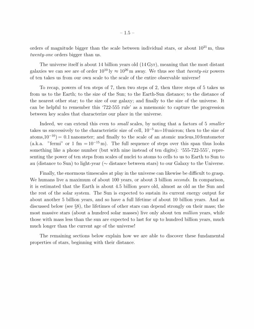
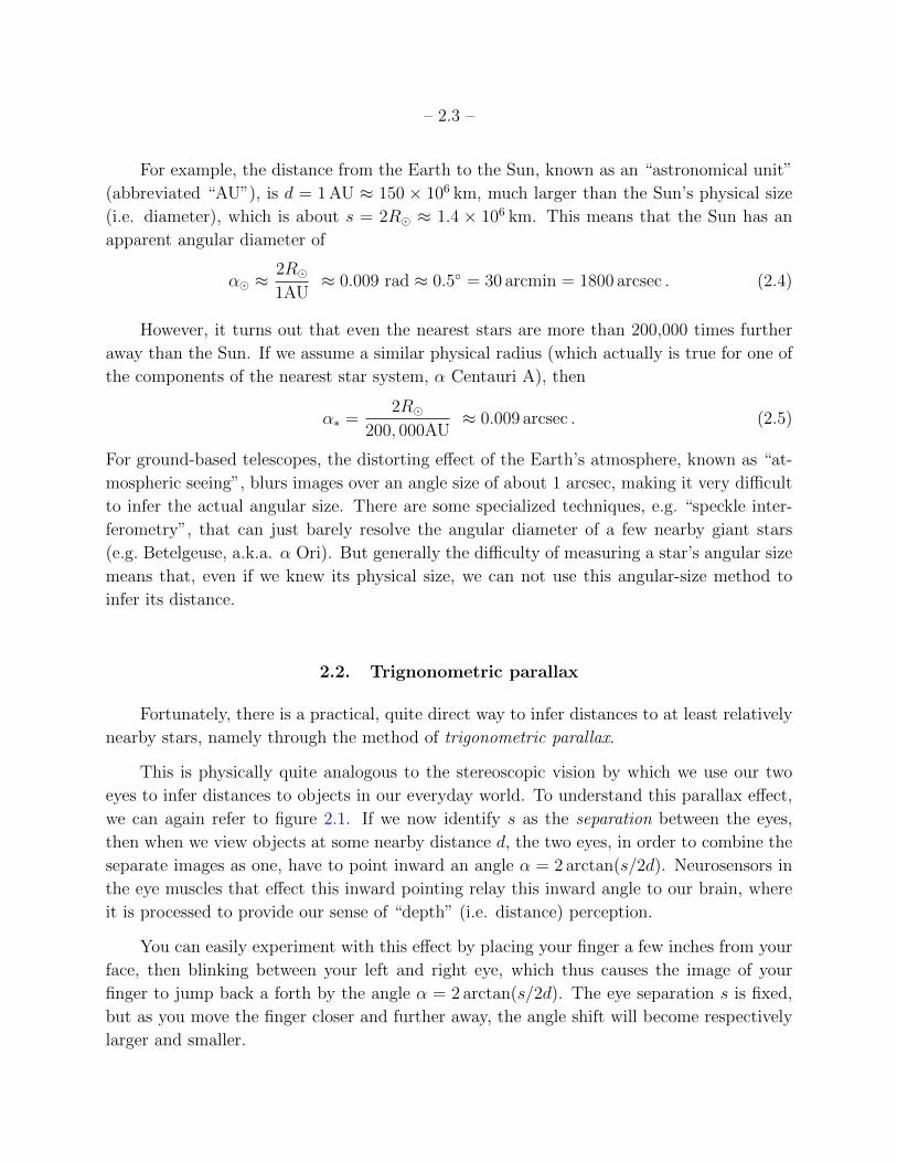
Fig. 2.1.— Angular size and parallax: The triangle illustrates how an object of physical
size s (BC) subtends an angular size α when viewed from a point A that is at a distance d.
Note that the same triangle can also illustrate the parallax angle α toward the point A at
distance d when viewed from two points B and C separated by a length s.
As illustrated in figure 2.1, we can, with the help of some elementary geometry, formalize
this intuition to write the specific formula. The triangle illustrates the angle α subtended
by an object of size s from a distance d. From simple trigonometry, we find
tan(α/2) =s/2
d. (2.1)
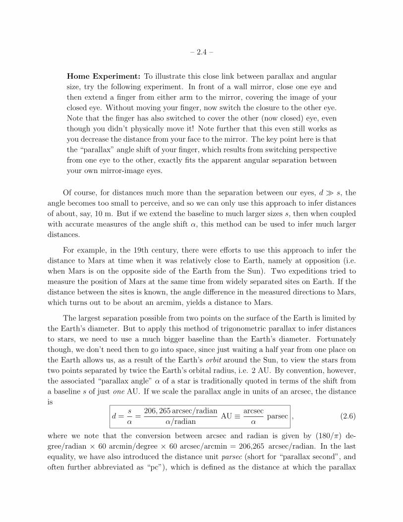
For distances much larger than the size, d s, the angle is small, α 1, for which
the tangent function can be approximated (e.g. by first-order Taylor expansion) to give
tan(α/2) ≈ α/2, where α is measured here in radians. (1 rad = (180/π) ≈ 57). The
relation between distance, size, and angle thus becomes simply
α ≈ s
d. (2.2)
– 2.2 –
0.2 0.6 1 1.4
0.5
1
1.5
2Tan x
Sin x
x
x
x+x3/3
x-x3/6
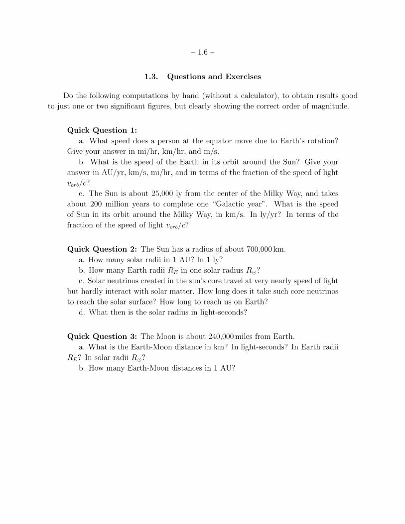
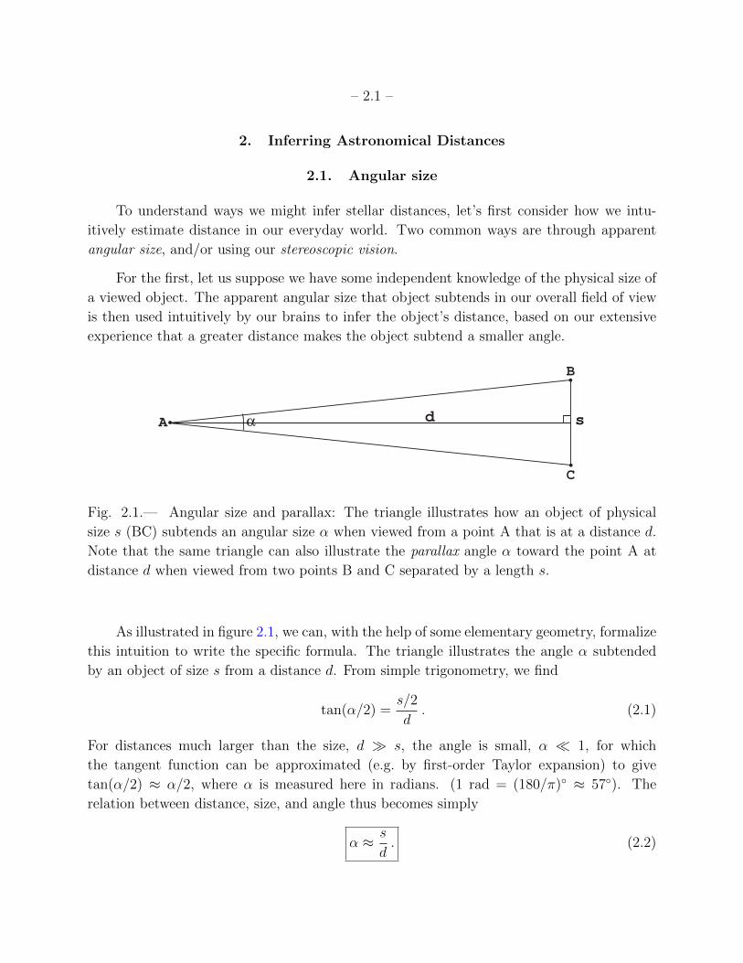
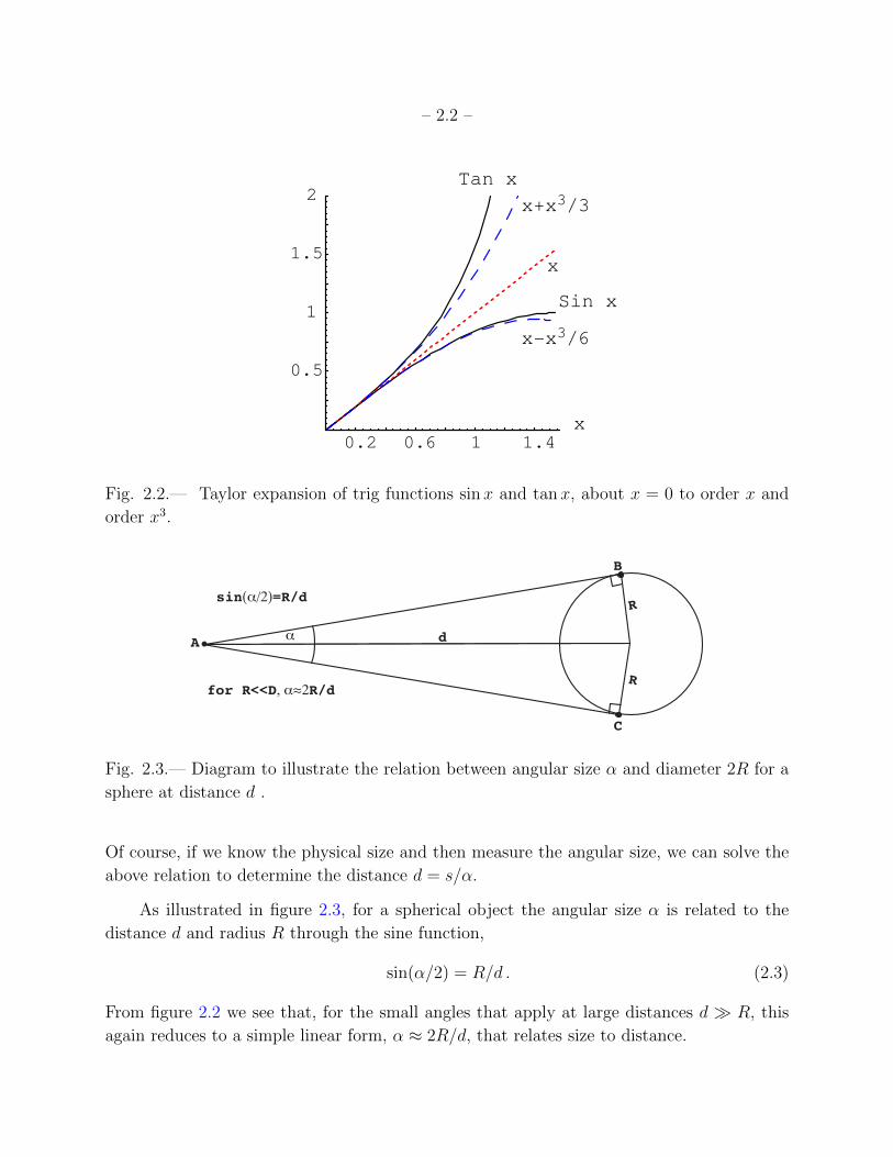
Fig. 2.2.— Taylor expansion of trig functions sinx and tan x, about x = 0 to order x and
order x3.
d
R
R
αA
B
C
sin(α/2)=R/d
for R<<D, α≈2R/d
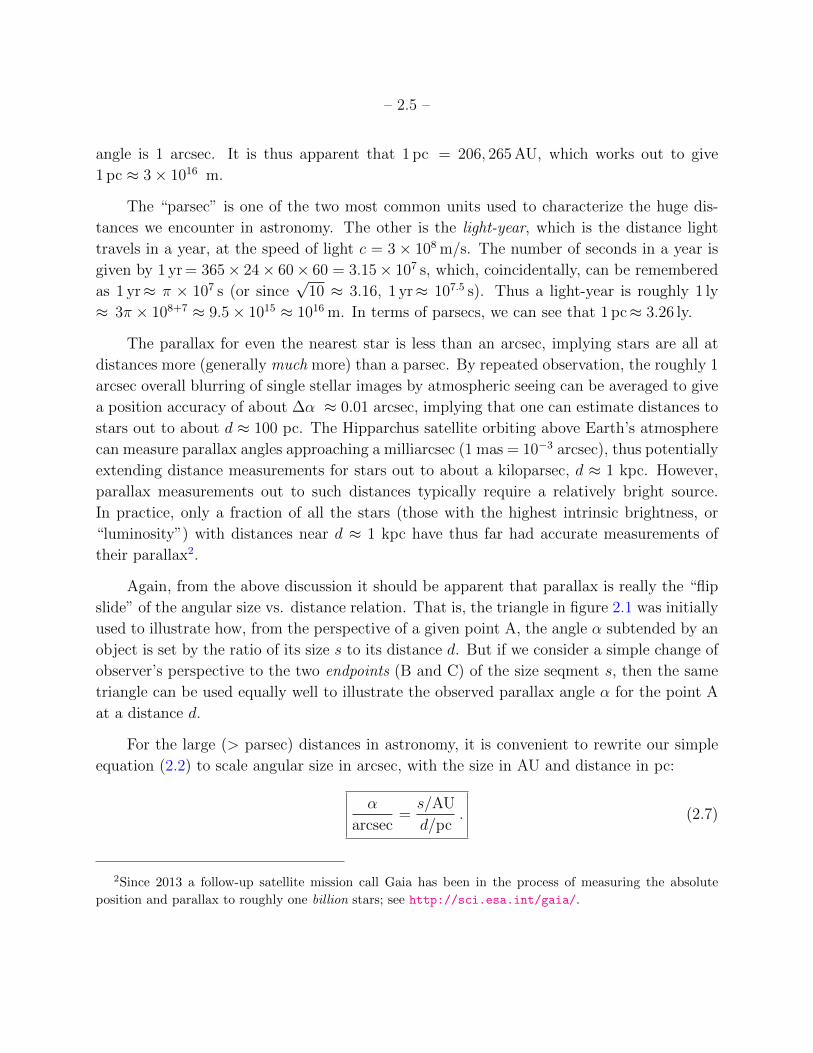
Fig. 2.3.— Diagram to illustrate the relation between angular size α and diameter 2R for a
sphere at distance d .
Of course, if we know the physical size and then measure the angular size, we can solve the
above relation to determine the distance d = s/α.
As illustrated in figure 2.3, for a spherical object the angular size α is related to the
distance d and radius R through the sine function,
sin(α/2) = R/d . (2.3)
From figure 2.2 we see that, for the small angles that apply at large distances d R, this
again reduces to a simple linear form, α ≈ 2R/d, that relates size to distance.
– 2.3 –
For example, the distance from the Earth to the Sun, known as an “astronomical unit”
(abbreviated “AU”), is d = 1 AU ≈ 150 × 106 km, much larger than the Sun’s physical size
(i.e. diameter), which is about s = 2R ≈ 1.4 × 10⁶ km. This means that the Sun has an
apparent angular diameter of
α ≈2R1AU
≈ 0.009 rad ≈ 0.5 = 30 arcmin = 1800 arcsec . (2.4)
However, it turns out that even the nearest stars are more than 200,000 times further
away than the Sun. If we assume a similar physical radius (which actually is true for one of
the components of the nearest star system, α Centauri A), then
α∗ =2R
200, 000AU≈ 0.009 arcsec . (2.5)
For ground-based telescopes, the distorting effect of the Earth’s atmosphere, known as “at-
mospheric seeing”, blurs images over an angle size of about 1 arcsec, making it very difficult
to infer the actual angular size. There are some specialized techniques, e.g. “speckle inter-
ferometry”, that can just barely resolve the angular diameter of a few nearby giant stars
(e.g. Betelgeuse, a.k.a. α Ori). But generally the difficulty of measuring a star’s angular size
means that, even if we knew its physical size, we can not use this angular-size method to
infer its distance.
2.2. Trignonometric parallax
Fortunately, there is a practical, quite direct way to infer distances to at least relatively
nearby stars, namely through the method of trigonometric parallax.
This is physically quite analogous to the stereoscopic vision by which we use our two
eyes to infer distances to objects in our everyday world. To understand this parallax effect,
we can again refer to figure 2.1. If we now identify s as the separation between the eyes,
then when we view objects at some nearby distance d, the two eyes, in order to combine the
separate images as one, have to point inward an angle α = 2 arctan(s/2d). Neurosensors in
the eye muscles that effect this inward pointing relay this inward angle to our brain, where
it is processed to provide our sense of “depth” (i.e. distance) perception.
You can easily experiment with this effect by placing your finger a few inches from your
face, then blinking between your left and right eye, which thus causes the image of your
finger to jump back a forth by the angle α = 2 arctan(s/2d). The eye separation s is fixed,
but as you move the finger closer and further away, the angle shift will become respectively
larger and smaller.
– 2.4 –
Home Experiment: To illustrate this close link between parallax and angular
size, try the following experiment. In front of a wall mirror, close one eye and
then extend a finger from either arm to the mirror, covering the image of your
closed eye. Without moving your finger, now switch the closure to the other eye.
Note that the finger has also switched to cover the other (now closed) eye, even
though you didn’t physically move it! Note further that this even still works as
you decrease the distance from your face to the mirror. The key point here is that
the “parallax” angle shift of your finger, which results from switching perspective
from one eye to the other, exactly fits the apparent angular separation between
your own mirror-image eyes.
Of course, for distances much more than the separation between our eyes, d s, the
angle becomes too small to perceive, and so we can only use this approach to infer distances
of about, say, 10 m. But if we extend the baseline to much larger sizes s, then when coupled
with accurate measures of the angle shift α, this method can be used to infer much larger
distances.
For example, in the 19th century, there were efforts to use this approach to infer the
distance to Mars at time when it was relatively close to Earth, namely at opposition (i.e.
when Mars is on the opposite side of the Earth from the Sun). Two expeditions tried to
measure the position of Mars at the same time from widely separated sites on Earth. If the
distance between the sites is known, the angle difference in the measured directions to Mars,
which turns out to be about an arcmim, yields a distance to Mars.
The largest separation possible from two points on the surface of the Earth is limited by
the Earth’s diameter. But to apply this method of trigonometric parallax to infer distances
to stars, we need to use a much bigger baseline than the Earth’s diameter. Fortunately
though, we don’t need then to go into space, since just waiting a half year from one place on
the Earth allows us, as a result of the Earth’s orbit around the Sun, to view the stars from
two points separated by twice the Earth’s orbital radius, i.e. 2 AU. By convention, however,
the associated “parallax angle” α of a star is traditionally quoted in terms of the shift from
a baseline s of just one AU. If we scale the parallax angle in units of an arcsec, the distance
is
d =s
α=
206, 265 arcsec/radian
α/radianAU ≡ arcsec
αparsec , (2.6)
where we note that the conversion between arcsec and radian is given by (180/π) de-
gree/radian × 60 arcmin/degree × 60 arcsec/arcmin = 206,265 arcsec/radian. In the last
equality, we have also introduced the distance unit parsec (short for “parallax second”, and
often further abbreviated as “pc”), which is defined as the distance at which the parallax
– 2.5 –
angle is 1 arcsec. It is thus apparent that 1 pc = 206, 265 AU, which works out to give
1 pc ≈ 3× 10¹⁶ m.
The “parsec” is one of the two most common units used to characterize the huge dis-
tances we encounter in astronomy. The other is the light-year, which is the distance light
travels in a year, at the speed of light c = 3× 10⁸ m/s. The number of seconds in a year is
given by 1 yr = 365× 24× 60× 60 = 3.15× 10⁷ s, which, coincidentally, can be remembered
as 1 yr≈ π × 107 s (or since√
10 ≈ 3.16, 1 yr≈ 107.5 s). Thus a light-year is roughly 1 ly
≈ 3π × 108+7 ≈ 9.5× 10¹⁵ ≈ 1016 m. In terms of parsecs, we can see that 1 pc≈ 3.26 ly.
The parallax for even the nearest star is less than an arcsec, implying stars are all at
distances more (generally much more) than a parsec. By repeated observation, the roughly 1
arcsec overall blurring of single stellar images by atmospheric seeing can be averaged to give
a position accuracy of about ∆α ≈ 0.01 arcsec, implying that one can estimate distances to
stars out to about d ≈ 100 pc. The Hipparchus satellite orbiting above Earth’s atmosphere
can measure parallax angles approaching a milliarcsec (1 mas = 10−3 arcsec), thus potentially
extending distance measurements for stars out to about a kiloparsec, d ≈ 1 kpc. However,
parallax measurements out to such distances typically require a relatively bright source.
In practice, only a fraction of all the stars (those with the highest intrinsic brightness, or
“luminosity”) with distances near d ≈ 1 kpc have thus far had accurate measurements of
their parallax2.
Again, from the above discussion it should be apparent that parallax is really the “flip
slide” of the angular size vs. distance relation. That is, the triangle in figure 2.1 was initially
used to illustrate how, from the perspective of a given point A, the angle α subtended by an
object is set by the ratio of its size s to its distance d. But if we consider a simple change of
observer’s perspective to the two endpoints (B and C) of the size seqment s, then the same
triangle can be used equally well to illustrate the observed parallax angle α for the point A
at a distance d.
For the large (> parsec) distances in astronomy, it is convenient to rewrite our simple
equation (2.2) to scale angular size in arcsec, with the size in AU and distance in pc:
α
arcsec=s/AU
d/pc. (2.7)
2Since 2013 a follow-up satellite mission call Gaia has been in the process of measuring the absolute
position and parallax to roughly one billion stars; see http://sci.esa.int/gaia/.
– 2.6 –
2.3. Determining the astronomical unit
We thus see that determining the distance of the Earth to the sun, i.e. measuring the
physical length of an AU, provides a fundamental basis for determining the distances to
stars and other objects in the universe. In modern times, one way this is computed involves
first measuring the distance from the Earth to the planet Venus though “radar ranging”, i.e.
measuring the time ∆t it takes a radar signal to bounce off Venus and return to Earth. The
associated Earth-Venus distance is then given by
dEV =∆t
2c. (2.8)
If this distance is measured at the time when Venus has its “maximum elongation”, or
maximum angular separation, from the sun, which is found to be about 47o, then one can
use simple trigonometry to derive a physical value of the AU. The details are left as an
exercise for the reader. (See Exercise 2-1 at the end of this section.)
2.4. Solid angle
In general objects that have a measurable angular size on the sky are extended in two
independent directions. As the 2D generalization of an angle along just one direction, it is
useful then to define for such objects a 2D solid angle Ω, measured now in square radians,
but more commonly referred by the shorthand “steradians”.
Just as projected area A is related to the square of physical size s (or radius R), so is
solid angle Ω related to the square of the angular size α. For an object at a distance d with
projected area A, the solid angle is just
Ω =A
d2≈ πR2
d2= πα2 , (2.9)
where the latter equalities assume a sphere (or disk) with projected radius R and associated
angular radius α = R/d.
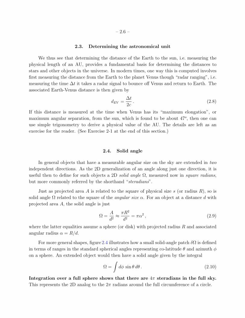
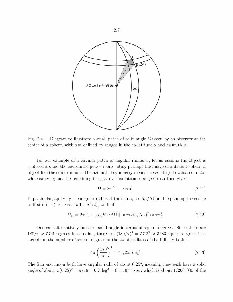
For more general shapes, figure 2.4 illustrates how a small solid-angle patch δΩ is defined
in terms of ranges in the standard spherical angles representing co-latitude θ and azimuth φ
on a sphere. An extended object would then have a solid angle given by the integral
Ω =
∫dφ sin θ dθ . (2.10)
Integration over a full sphere shows that there are 4π steradians in the full sky.
This represents the 2D analog to the 2π radians around the full circumference of a circle.
– 2.7 –
θ
θ+δθ
δφδΩ=sinθ δθ δφ
Fig. 2.4.— Diagram to illustrate a small patch of solid angle δΩ seen by an observer at the
center of a sphere, with size defined by ranges in the co-latitude θ and azimuth φ.
For our example of a circular patch of angular radius α, let us assume the object is
centered around the coordinate pole – representing perhaps the image of a distant spherical
object like the sun or moon. The azimuthal symmetry means the φ integral evaluates to 2π,
while carrying out the remaining integral over co-latitude range 0 to α then gives
Ω = 2π [1− cosα] . (2.11)
In particular, applying the angular radius of the sun α ≈ R/AU and expanding the cosine
to first order (i.e., cosx ≈ 1− x2/2), we find
Ω = 2π [1− cos(R/AU)] ≈ π(R/AU)2 ≈ πα2 . (2.12)
One can alternatively measure solid angle in terms of square degrees. Since there are
180/π ≈ 57.3 degrees in a radian, there are (180/π)2 = 57.32 ≈ 3283 square degrees in a
steradian; the number of square degrees in the 4π steradians of the full sky is thus
4π
(180
π
)2
= 41, 253 deg2 . (2.13)
The Sun and moon both have angular radii of about 0.25o, meaning they each have a solid
angle of about π(0.25)2 = π/16 = 0.2 deg2 = 6× 10⁻⁵ ster, which is about 1/200, 000 of the
– 2.8 –
full sky3.
2.5. Questions and Exercises
Quick Question 1: A helium party balloon of diameter 20 cm floats 1 meter
above your head.
a. What is its angular diameter, in degrees and radians?
b. What is its solid angle, in square degrees and steradians?
c. What fraction of the full sky does it cover?
d. At what height h would its angular diameter equal that of the Moon and
Sun?
Quick Question 2:
a. What angle α would the Earth-Sun separation subtend if viewed from a
distance of d = 1 pc? Give your answer in both radian and arcsec.
b. How about from a distance of d = 1 kpc?
Quick Question 3: Over a period of several years, two stars appear to go
around each other with a fixed angular separation of 1 arcsec.
a. What is the physical separation, in au, between the stars if they have a
distance d = 10 pc from Earth?
b. If they have a distance d = 100 pc?
Exercise 1: At the time when Venus exhibits its maximum elongation angle
of about 47o from the Sun, a radar signal is found to take a round trip time
∆t = 667 sec to return to Earth. Assuming both Earth and Venus have circular
orbits, and using the speed of light c = 3 × 10⁵ km/s, compute (in km) the
Earth-Sun distance, 1 AU.
Exercise 2: With a sufficiently large telescope in space, with angle error ∆α ≈1 mas, for how many more stars can we expect to obtain a measured parallax than
we can from ground-based surveys with ∆α ≈ 20 mas? (Hint: What assumption
do you need to make about the space density of stars in the region of the galaxy
within 1 kpc from the Sun/Earth?)
3If you think about it, you’ll see that this helps explain why a full moon is about a million times dimmer
than full sunlight! See Exercise 2-3.

– 2.9 –
Exercise 3: a. Assuming the Moon reflects a fraction a (dubbed the “albedo”)
of sunlight hitting it, derive an expression for the ratio of apparent brightness
(Fmoon/F) between the full Moon and Sun, in terms of the Moon’s radius Rmoon
and its distance from earth, dem au. b. Derive the value of the albedo a for
which this ratio equals the fraction of sky subtended by the Moon’s solid angle,
i.e. for which Fmoon/F = Ωmoon/4π.

– 3.1 –
3. Inferring Stellar Luminosity
3.1. “Standard Candle” methods for distance
In our everyday experience, there is another way we sometimes infer distance, namely
by the change in apparent brightness for objects that emit their own light, with some known
power or “luminosity”. For example, a hundred watt light bulb at a distance of d = 1 m
certainly appears a lot brighter than that same bulb at d = 100 m. Just as for a star, what
we observe as apparent brightness is really a measure of the flux of light, i.e. energy per unit
time per unit area (erg/s/cm2 in CGS units, or watt/m2 in MKS).
When viewing a light bulb with our eyes, it’s just the rate at which the light’s energy is
captured by the area of our pupils. If we assume the light bulb’s emission is isotropic (i.e.,
the same in all directions), then as the light travels outward to a distance d, its power or
luminosity is spread over a sphere of area 4πd2. This means that the light detected over a
fixed detector area (like the pupil of our eye, or, for telescopes observing stars, the area of
the telescope mirror) decreases in proportion to the inverse-square of the distance, 1/d2. We
can thus define the apparent brightness in terms of the flux,
F =L
4πd2. (3.1)
This is a profoundly important equation in astronomy, and so you should not just memorize
it, but embed it completely and deeply into your psyche.
In particular, it should become obvious that this equation can be readily used to infer the
distance to an object of known luminosity, an approach called the standard candle method.
(Taken from the idea that a candle, or at least a “standard” candle, has a known luminosity
or intrinisic brightness.) As discussed further in sections below, there are circumstances in
which we can get clues to a star’s (or other object’s) intrinsic luminosity L, for example
through careful study of a star’s spectrum. If we then measure the apparent brightness (i.e.
flux F ), we can infer the distance through:
d =
√L
4πF. (3.2)
Indeed, when the study of a stellar spectrum is the way we infer the luminosity, this method
of distance determination is sometimes called “spectroscopic parallax”.
Of course, if we can independently determine the distance through the actual trigono-
metric parallax, then such a simple measurement of the flux can instead be used to determine
the luminosity,
L = 4πd2 F . (3.3)
– 3.2 –
In the case of the Sun, the flux measured at Earth is referred to as the “solar constant”,
with a measured mean value of about
F ≈ 1.4kW
m2= 1.4× 10⁶ erg
cm2 s. (3.4)
If we then apply the known mean distance of the Earth to the Sun, d = 1 au, we obtain for
the solar luminosity
L ≈ 4× 1026W = 4× 1033 erg
s. (3.5)
Thus we see that the Sun emits the power of about 4×1024 100-watt light bulbs! In common
language this corresponds to four million billion billion, a number so huge that it loses any
meaning. It illustrates again how in astronomy we have to think on a entirely different scale
than we are used to in our everyday world.
But once we get used to the idea that the luminosity and other properties of the Sun
are huge but still finite and measurable, we can use these as benchmarks for characterizing
analogous properties of other stars and astronomical objects. In the case of stellar luminosi-
ties, for example, these typically range from about L/1000 for very cool, low-mass “dwarf”
stars, to as high as 106L for very hot, high-mass “supergiants”.
As discussed further below, the luminosity of a star depends directly on both its size
(i.e. radius) and surface temperature. But more fundamentally these in turn are largely set
by the star’s mass, age, and chemical composition.
3.2. Intensity or Surface Brightness
For any object with a resolved solid angle Ω, an important flux-related quantity is the
surface brightness – also known as the specific intensity I (see §12.1); this can be thought of
as the flux per solid angle, i.e.
I ≈ F
Ω≈ L
4πd2π(R/d)2≈ L
4π2R2=F∗π, (3.6)
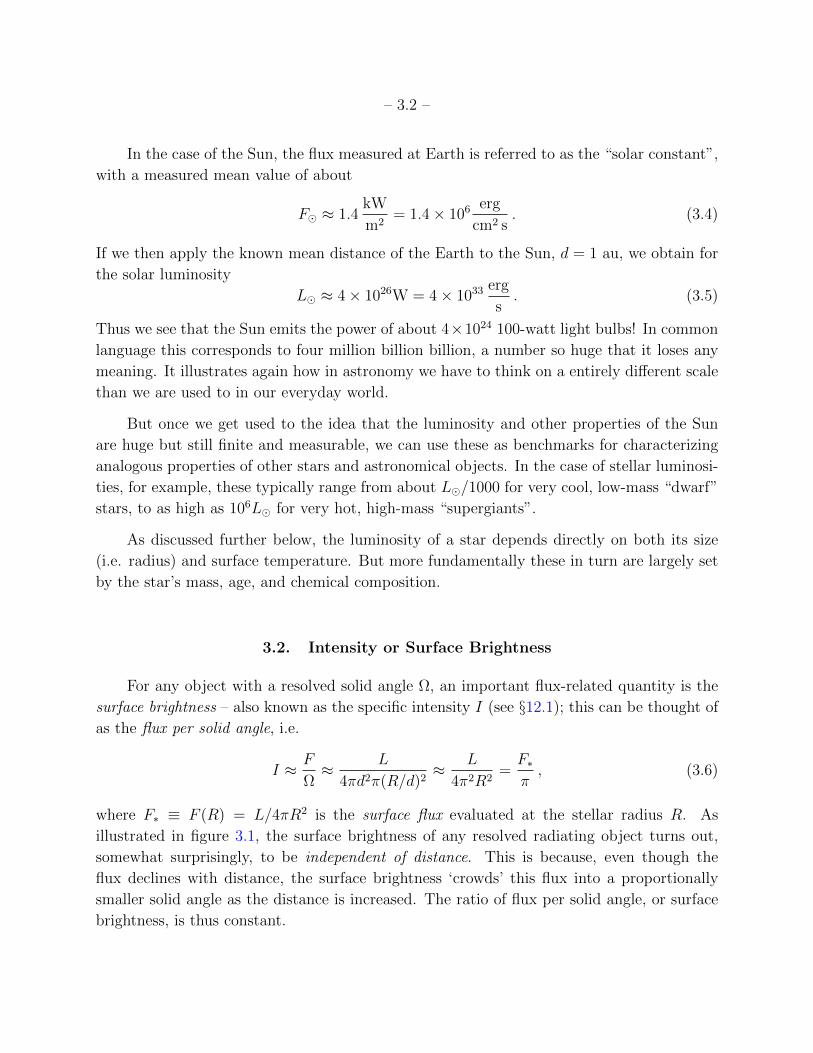
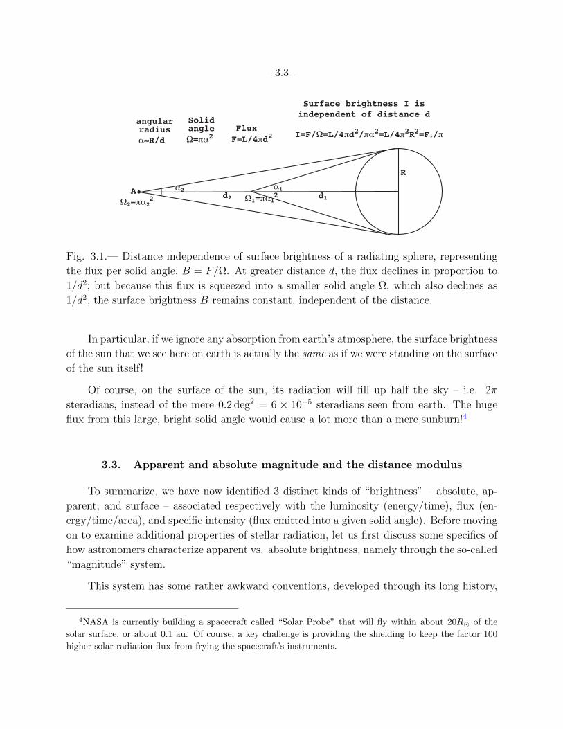
where F∗ ≡ F (R) = L/4πR2 is the surface flux evaluated at the stellar radius R. As
illustrated in figure 3.1, the surface brightness of any resolved radiating object turns out,
somewhat surprisingly, to be independent of distance. This is because, even though the
flux declines with distance, the surface brightness ‘crowds’ this flux into a proportionally
smaller solid angle as the distance is increased. The ratio of flux per solid angle, or surface
brightness, is thus constant.
– 3.3 –
d1A d2
α2
Ω2=πα22
α1
R
Ω1=πα12
Ω=πα2α≈R/d F=L/4πd2 I=F/Ω=L/4πd2/πα2=L/4π2R2=F*/π
Surface brightness I isindependent of distance d
angularradius
Solidangle Flux
Fig. 3.1.— Distance independence of surface brightness of a radiating sphere, representing
the flux per solid angle, B = F/Ω. At greater distance d, the flux declines in proportion to
1/d2; but because this flux is squeezed into a smaller solid angle Ω, which also declines as
1/d2, the surface brightness B remains constant, independent of the distance.
In particular, if we ignore any absorption from earth’s atmosphere, the surface brightness
of the sun that we see here on earth is actually the same as if we were standing on the surface
of the sun itself!
Of course, on the surface of the sun, its radiation will fill up half the sky – i.e. 2π
steradians, instead of the mere 0.2 deg2 = 6 × 10⁻⁵ steradians seen from earth. The huge
flux from this large, bright solid angle would cause a lot more than a mere sunburn!4
3.3. Apparent and absolute magnitude and the distance modulus
To summarize, we have now identified 3 distinct kinds of “brightness” – absolute, ap-
parent, and surface – associated respectively with the luminosity (energy/time), flux (en-
ergy/time/area), and specific intensity (flux emitted into a given solid angle). Before moving
on to examine additional properties of stellar radiation, let us first discuss some specifics of
how astronomers characterize apparent vs. absolute brightness, namely through the so-called
“magnitude” system.
This system has some rather awkward conventions, developed through its long history,
4NASA is currently building a spacecraft called “Solar Probe” that will fly within about 20R of the
solar surface, or about 0.1 au. Of course, a key challenge is providing the shielding to keep the factor 100
higher solar radiation flux from frying the spacecraft’s instruments.
– 3.4 –
dating back to the ancient Greeks. As noted in the Introduction, they ranked the apparent
brightness of stars in 6 bins of magnitude, ranging from m = 1 for the brightest to m = 6
for the dimmest. Because the human eye is adapted to detect a large dynamic range in
brightness, it turns out that our perception of brightness depends roughly on the logarithm
of the flux.
In our modern calibration this can be related to the Greek magnitude system by stating
that a difference of 5 in magnitude represents a factor 100 in the relative brightness of the
compared stars, with the dimmer star having the larger magnitude. This can be expressed
in mathematical form as
m2 −m1 = 2.5 log(F1/F2) . (3.7)
We can further extend this logarithmic magnitude system to characterize the absolute
brightness, a.k.a. luminosity, of a star in terms of an absolute magnitude. To remove the
inherent dependence on distance in the flux F , and thus in the apparent magnitude m, the
absolute magnitude M is defined as the apparent magnitude that a star would have if it were
placed at a standard distance, chosen by convention to be d = 10 pc. Since the flux scales
with the inverse-square of distance, F ∼ 1/d2, the difference between apparent magnitude
m and absolute magnitude M is given by
m−M = 5 log(d/10 pc) , (3.8)
which is known as the distance modulus.
The absolute magnitude of the Sun is M ≈ +4.8 (though for simplicity in calculations,
this is often rounded up to 5), and so the scaling for other stars can be written as
M = 4.8− 2.5 log(L/L) . (3.9)
Combining these relations, we see that the apparent magnitude of any star is given in terms
of the luminosity and distance by
m = 4.8− 2.5 log(L/L) + 5 log(d/10 pc) . (3.10)
For bright stars, magnitudes can even become negative. For example, the (apparently)
brightest star in the night sky, Sirius, has an apparent magnitude m = −1.42. But with
a luminosity of just L ≈ 23L, its absolute magnitude is still positive, M = +1.40. Its
distance modulus, m −M = −1.42 − 1.40 = −2.82, is negative. Through eqn. (3.8), this
implies that its distance, d = 101−2.82/5 = 2.7 pc, is less than the standard distance of 10 pc
used to define absolute magnitude and distance modulus [eqn. (3.8)].
– 3.5 –
3.4. Questions and Exercises
Quick Question 1: Recalling the relationship between an AU and a parsec
from eqn. (2.6), use eqns. (3.8) and (3.9) to compute the apparent magnitude of
the sun. What then is the sun’s distance modulus?
Quick Question 2: Suppose two stars have a luminosity ratio L2/L1 = 100.
a. At what distance ratio d2/d1 would the stars have the same apparent
brightness, F2 = F1?
b. For this distance ratio, what is the difference in their apparent magnitude,
m2 −m1?
c. What is the difference in their absolute magnitude, M2 −M1?
d. What is the difference in their distance modulus?
Quick Question 3: A white-dwarf-supernova with peak luminosity L ≈ 1010 Lis observed to have an apparent magnitude of m = +20 at this peak.
a. What is its Absolute Magnitude M?
b. What is its distance d (in pc and ly).
c. How long ago did this supernova explode (in Myr)?
(For simplicity of computation, you may take the absolute magnitude of the
sun to be M ≈ +5.)
– 4.1 –
4. Inferring Surface Temperature from a Star’s Color and/or Spectrum
Let us next consider why stars shine with such extreme brightness. Over the long-term
(i.e., millions of years), the enormous energy emitted comes from the energy generated (by
nuclear fusion) in the stellar core, as discussed further below. But the more immediate reason
stars shine is more direct, namely because their surfaces are so very hot. The light they emit
is called “thermal radiation”, and arises from the jostling of the atoms (and particularly the
electrons in and around those atoms) by the violent collisions associated with the star’s high
temperature5.
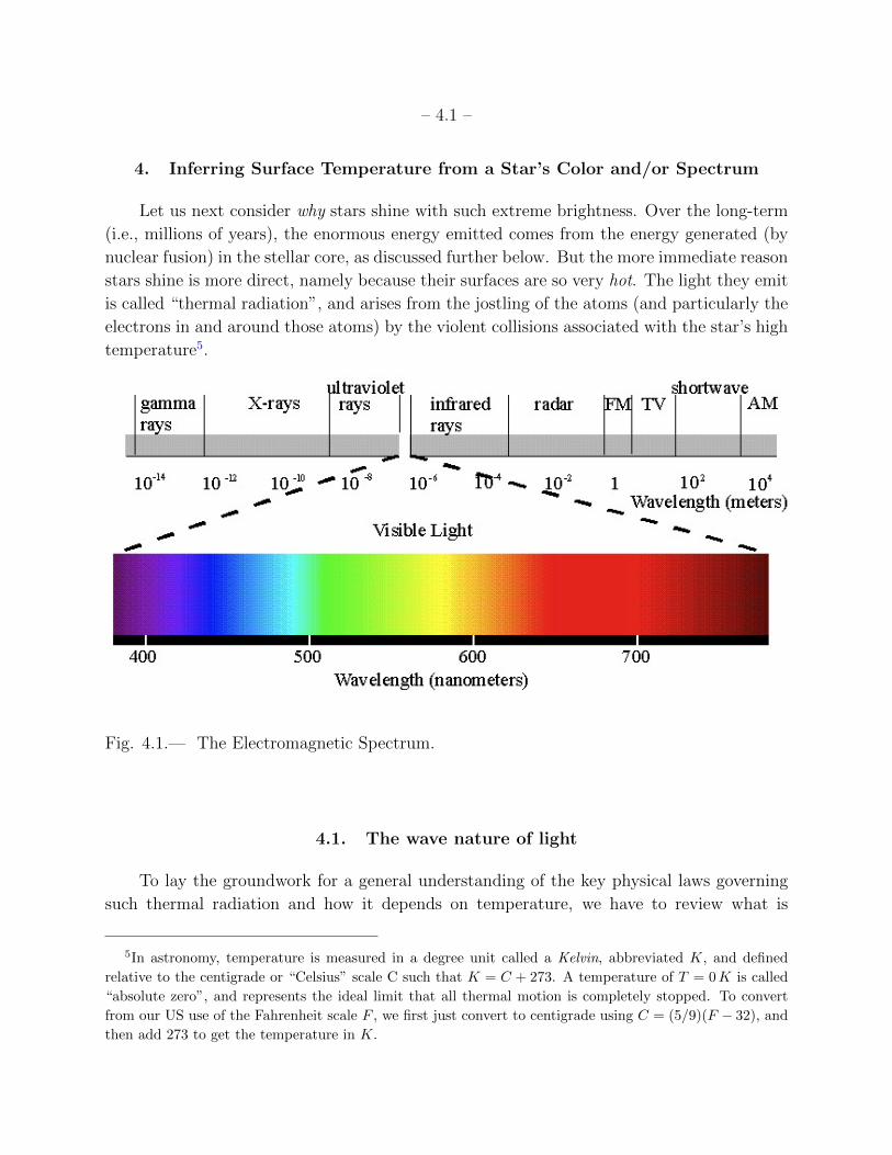
Fig. 4.1.— The Electromagnetic Spectrum.
4.1. The wave nature of light
To lay the groundwork for a general understanding of the key physical laws governing
such thermal radiation and how it depends on temperature, we have to review what is
5In astronomy, temperature is measured in a degree unit called a Kelvin, abbreviated K, and defined
relative to the centigrade or “Celsius” scale C such that K = C + 273. A temperature of T = 0K is called
“absolute zero”, and represents the ideal limit that all thermal motion is completely stopped. To convert
from our US use of the Fahrenheit scale F , we first just convert to centigrade using C = (5/9)(F − 32), and
then add 273 to get the temperature in K.
– 4.2 –
understood about the basic nature of light, and the processes by which it is emitted and
absorbed.
The 19th century physicist James Clerk Maxwell developed a set of 4 equations (Maxwell’s
equations) that showed how variations in Electric and Magnetic fields could lead to oscillat-
ing wave solutions, which he indeed indentifed with light, or more generally Electro-Magnetic
(EM) radiation. The wavelengths λ of these EM waves are key to their properties. As illus-
trated in figure 4.1, visible light corresponds to wavelengths ranging from λ ≈ 400 nm (violet)
to λ ≈ 750 nm (red), but the full spectrum extends much further, including Ultra-Violet
(UV), X-rays, and gamma rays at shorter wavelengths, and InfraRed (IR), microwaves, and
radio waves at longer wavelengths. White light is made up of a broad mix of visible light
ranging from Red through Green to Blue (RGB).
In a vacuum, all these EM waves travel at the same speed, namely the speed of light,
customarily denoted as c, with a value c ≈ 3× 10⁵ km/s = 3× 10⁸ m/s = 3× 1010 cm/s. The
wave period is the time it takes for a complete wavelength to pass a fixed point at this speed,
and so is given by P = λ/c. We can thus see that the sequence of wave crests passes by
at a frequency of once per period, ν = 1/P , implying a simple relationship between light’s
wavelength λ, frequency ν, and speed c,
λ
P= λν = c . (4.1)
4.2. Light quanta and the Black-Body emission spectrum
The wave nature of light has been confirmed by a wide range experiments. However, at
the beginning of the 20th century, work by Einstein, Planck, and others led to the realization
that light waves are also quantized into discrete wave “bundles” called photons, each of which
carries a discrete, indivisible “quantum” of energy that depends on the wave frequency as
E = hν , (4.2)
where h is Planck’s constant, with value h ≈ 6.6× 10⁻²⁷ erg s = 6.6× 10⁻³⁴ Joule s.
This quantization of light (and indeed of all energy) has profound and wide-ranging
consequences, most notably in the current context for how thermally emitted radiation is
distributed in wavelength or frequency. This is known as the “Spectral Energy Distribution”
(SED). For a so-called Black Body – meaning idealized material that is readily able to absorb
and emit radiation of all wavelengths –, Planck showed that as thermal motions of the
– 4.3 –
Bλλ
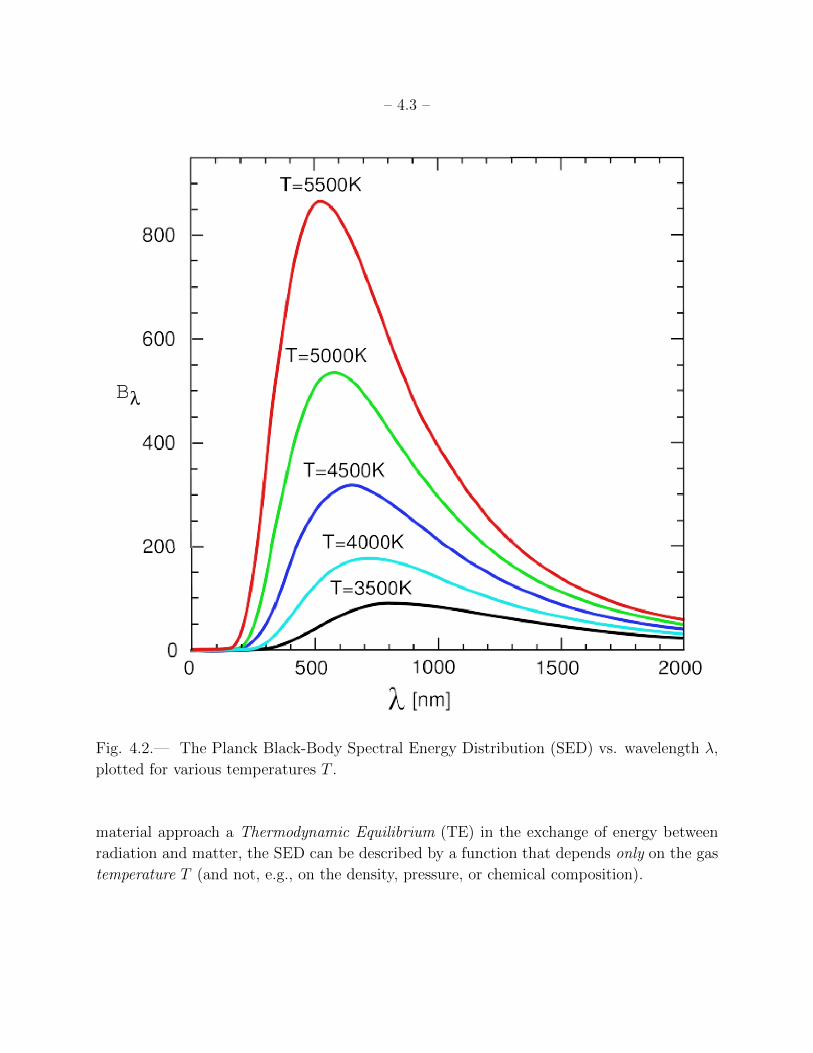
Fig. 4.2.— The Planck Black-Body Spectral Energy Distribution (SED) vs. wavelength λ,
plotted for various temperatures T .
material approach a Thermodynamic Equilibrium (TE) in the exchange of energy between
radiation and matter, the SED can be described by a function that depends only on the gas
temperature T (and not, e.g., on the density, pressure, or chemical composition).
– 4.4 –
In terms of the wave frequency ν, this Planck Black-Body function takes the form
Bν(T ) =2hν3/c2
ehν/kT − 1, (4.3)
where k is Boltzmann’s constant, with value k = 1.38×10⁻¹⁶ erg/K = 1.38×10⁻²³ Joule/K.
For an interval of frequency between ν and ν + dν, the quantity Bνdν gives the emitted
energy per unit time per unit area per unit solid angle. This means the Planck Black-Body
function is fundamentally a measure of intensity or surface brightness, with Bν representing
the distribution of surface brightness over frequency ν, having CGS units erg/cm2/s/ster/Hz
(and MKS units W/m2/ster/Hz).
Sometimes it is convenient to instead define this Planck distribution in terms of the
brightness distribution in a wavelength interval between λ and λ+dλ, Bλdλ. Requiring that
this equals Bνdν, and noting that ν = c/λ implies |dν/dλ| = c/λ2, we can use eqn. (4.3) to
obtain
Bλ(T ) =2hc2/λ5
ehc/λkT − 1. (4.4)
4.3. Inverse-temperature dependence of wavelength for peak flux
Figure 4.2 plots the variation of Bλ vs. wavelength λ for various temperatures T . Note
that for higher temperature, the level of Bλ is higher at all wavelengths, with greatest
increases near the peak level.
Moreover, the location of this peak shifts to shorter wavelength with higher temperature.
We can determine this peak wavelength λmax by solving the equation[dBλ
dλ
]λ=λmax
≡ 0 . (4.5)
Leaving the details as an exercise, the result is
λmax =2.9× 10⁶ nm K
T=
290 nm
T/10, 000K≈ 500 nm
T/T, (4.6)
which is known as Wien’s displacement law.
For example, the last equality uses the fact that the observed wavelength peak in the
Sun’s spectrum is λmax, ≈ 500 nm, very near the the middle of the visible spectrum.6 We
6 This is not entirely coincidental, since our eyes evolved to use the wavelengths of light for which the
solar illumination is brightest.
– 4.5 –
can solve for a Black-Body-peak estimate for the Sun’s surface temperature
T =2.9× 10⁶ nm K
500 nm= 5800K . (4.7)
By similarly measuring the peak wavelength λmax in other stars, we can likewise derive an
estimate of their surface temperature by
T = Tλmax,λmax
≈ 5800K500 nm
λmax. (4.8)
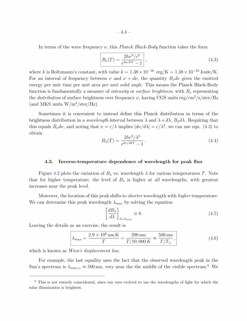
Fig. 4.3.— Comparison of the spectral sensitivity of the human eye with those the UBV
filters in the Johnson photometric color system.
4.4. Inferring stellar temperatures from photometric colors
In practice, this is not quite the approach that is most commonly used in astronomy,
in part because with real SEDs, it is relatively difficult to identify accurately the peak
wavelength. Moreover in surveying a large number of stars, it requires a lot more effort (and
telescope time) to measure the full SED, especially for relatively faint stars. A simpler, more
common method is just to measure the stellar color.
But rather than using the Red, Green, and Blue (RGB) colors we perceive with our eyes,
astronomers typically define a set of standard colors that extend to wavebands beyond just
the visible spectrum. The most common example is the Johnson 3-color UBV (Ulraviolet,
– 4.6 –
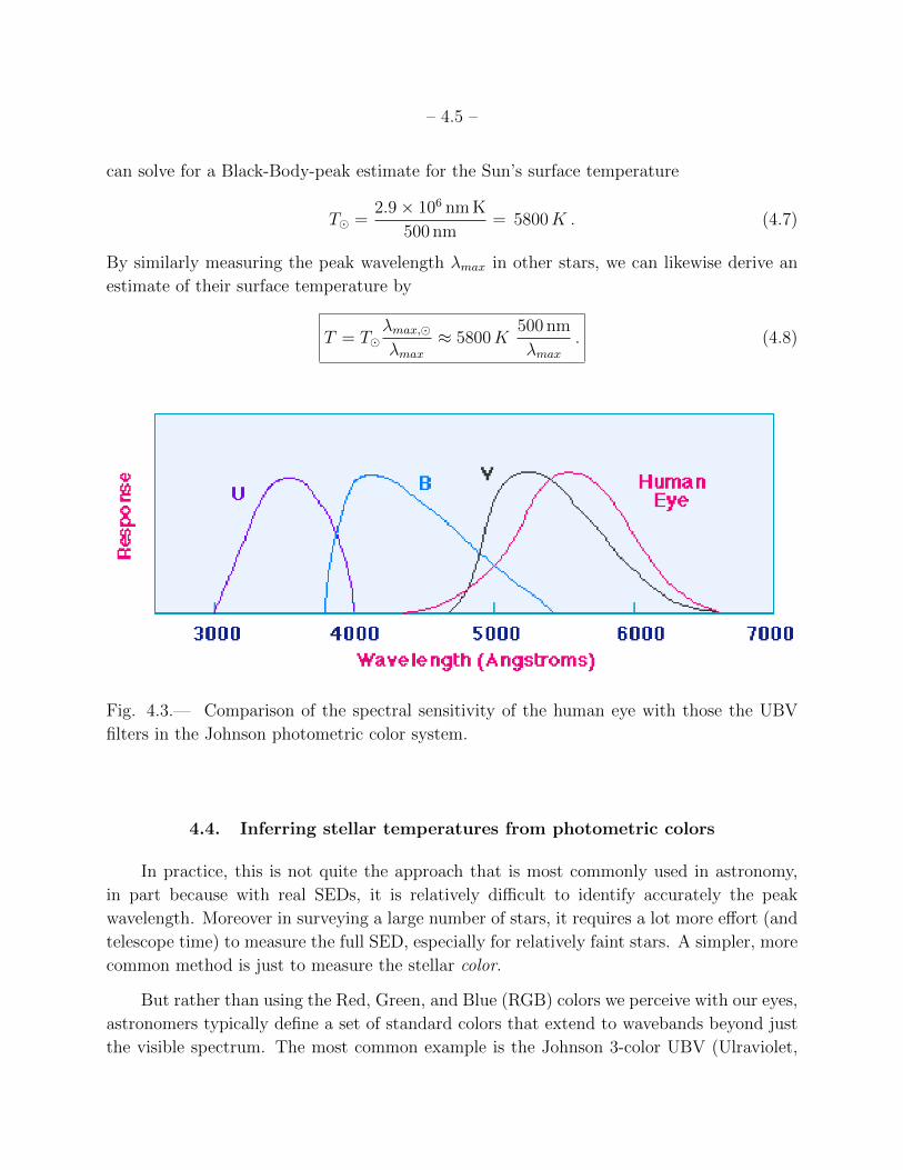
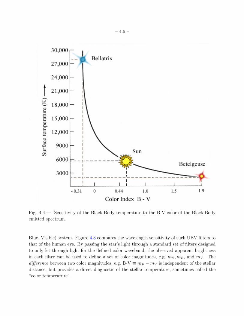
Fig. 4.4.— Sensitivity of the Black-Body temperature to the B-V color of the Black-Body
emitted spectrum.
Blue, Visible) system. Figure 4.3 compares the wavelength sensitivity of such UBV filters to
that of the human eye. By passing the star’s light through a standard set of filters designed
to only let through light for the defined color waveband, the observed apparent brightness
in each filter can be used to define a set of color magnitudes, e.g. mU ,mB, and mV . The
difference between two color magnitudes, e.g. B-V ≡ mB −mV is independent of the stellar
distance, but provides a direct diagnostic of the stellar temperature, sometimes called the
“color temperature”.
– 4.7 –
Because a larger magnitude corresponds to a lower brightness, stars with a positive B-V
actually are less bright in the blue than in the visible, implying a relatively low temperature.
On the other hand, a negative B-V means blue is brighter, implying a high temperature.
Figure 4.4 shows how the temperature of a Black-Body varies with the B-V color of the
emitted Black-Body spectrum. There is also a java applet that allows one to calculate the
sensitivity of various UBV color differences to Black-Body temperature, available at:
http://csep10.phys.utk.edu/astr162/lect/light/wien.html
4.5. Questions and Exercises
Quick Question 1: Two photons have wavelength ratio λ2/λ1 = 2.
a. What is the ratio of their period P2/P1?
b. What is the ratio of their frequency ν2/ν1?
c. What is the ratio of their energy E2/E1?
Quick Question 2:
a. Estimate the temperature of stars with λmax =100, 300, 1000, and 3000 nm.
(To simplify the numerics, you may take T ≈ 6000 K.)
b. Conversely, estimate the peak wavelengths λmax of stars with T =2000,
10,000, and 60, 000 K.
c. What parts of the EM spectrum (i.e. UV, visible, IR) do each of these lie
in?
Quick Question 3:
a. Assuming the earth has an average temperature equal to that of typi-
cal spring day, i.e. 50F, compute the peak wavelength of Earth’s Black-Body
radiation.
b. What part of the EM spectrum does this lie in?
Exercise 1: Using Bνdν = Bλdλ and the relationship between frequency ν
and wavelength λ, derive eqn. (4.4) from eqn. (4.3).
Exercise 2: Derive eqn. (4.6) from eqn. (4.4) using the definition (4.5).
– 5.1 –
5. Inferring Stellar Radius from Luminosity and Temperature
We see from figure 4.2 that, in addition to a shift toward shorter peak wavelength
λmax, a higher temperature also increases the overall brightness of blackbody emission at
all wavelengths. This suggests that the total energy emitted over all wavelengths should
increase quite sharply with temperature. Leaving the details as an exercise for the reader,
let us quantify this expectation by carrying out the necessary spectral integrals to obtain
the temperature dependence of the Bolometric intensity of a blackbody
B(T ) ≡∫ ∞
0
Bλ(T ) dλ =
∫ ∞0
Bν(T ) dν =σsbT
4
π, (5.1)
with σsb = 2π5k4/(15h3c2) known as the Stefan-Boltzmann constant, with numerical value
σsb = 5.67× 10⁻⁵ erg/cm2/s/K4 = 5.67× 10⁻⁸ J/m2/s/K4.
If we spatially resolve a pure blackbody with surface temperature T , then B(T ) repre-
sents the surface brightness we would observe from each part of the visible surface.
5.1. Stefan-Boltzmann law for surface flux from a blackbody
Combining eqns. (3.6) and (5.1), we see that the radiative flux at the surface radius R
of a blackbody is given by
F∗ ≡ F (R) = π B(T ) = σsbT4 , (5.2)
which is known as the Stefan-Boltzman law.
The Stefan-Boltzmann law is one of the linchpins of stellar astronomy. If we now relate
the surface flux to the stellar luminosity L over the surface area 4πR2, then applying this to
the Stefan-Boltzmann law gives
L = σsbT4 4πR2 , (5.3)
which is often convenient cast in terms of associated solar values,
L
L=
(T
T
)4 (R
R
)2
. (5.4)
We can also use eqn. (5.3) to solve for the stellar radius,
R =
√L
4πσsbT 4=
√F (d)
σsbT 4d , (5.5)
– 5.2 –
where the latter equation uses the inverse-square-law to relate the stellar radius to the flux
F (d) and distance d, along with the surface temperature T .
For a star with a known distance d, e.g. by a measured parallax, measurement of ap-
parent magnitude gives the flux F (d), while measurement of the peak wavelength λmax or
color (e.g. B-V) provides an estimate of the temperature T (see figure 4.4). Applying these
in eqn. (5.5), we can thus obtain an estimate of the stellar radius R.
5.2. Questions and Exercises
Quick Question 1: Compute the luminosity L (in units of the solar luminosity
L), absolute magnitude M , and peak wavelength λmax (in nm) for stars with
(a) T = T; R = 10R, (b) T = 10T; R = R, and (c) T = 10T; R = 10R.
If these stars all have a parallax of p = 0.001 arcsec, compute their associated
apparent magnitudes m.
Quick Question 2: Suppose a star has a parallax p = 0.01 arcsec, peak wave-
length λmax = 250 nm, and apparent magnitude m = +5 . About what is its:
a. Distance d (in pc)?
b. Distance modulus m−M?
c. Absolute magntidue M?
d. Luminosity L (in L)?
e. Surface temperature T (in T)?
f. Radius R (in R)?
g. Angular radius α (in radian and arcsec)?
h. Solid angle Ω (in steradian and arcsec2)?
i. Surface brightness relative to that of the Sun, B/B?

– 6.1 –
6. Absorption Lines in Stellar Spectra
Fig. 6.1.— The sun’s spectrum, showing the complex pattern of absorption lines at discrete
wavelength or colors.
In reality stars are not perfect blackbodies, and so their emitted spectra don’t just
depend on temperature, but contain detailed signatures of key physical properties like ele-
mental composition. The energy we see emitted from a stellar surface is generated in the
very hot interior and then diffuses outward, following the strong temperature decline to the
surface. The atoms and ions that absorb and emit the light don’t do so with perfect efficiency
at all wavelengths, which is what is meant by the “black” in “blackbody”. We experience
this all the time in our everyday world, which shows that different objects have distinct
“color”, meaning they absorb certain wavebands of light, and reflect others. For example, a
green leaf reflects some of the “green” parts of the visible spectrum – with wavelengths near
λ ≈ 5100 A– and absorbs most of the rest.
For atoms in a gas, the ability to absorb, scatter and emit light can likewise depend
on the wavelength, sometimes quite sharply. Just as the energy of light is quantized into
– 6.2 –
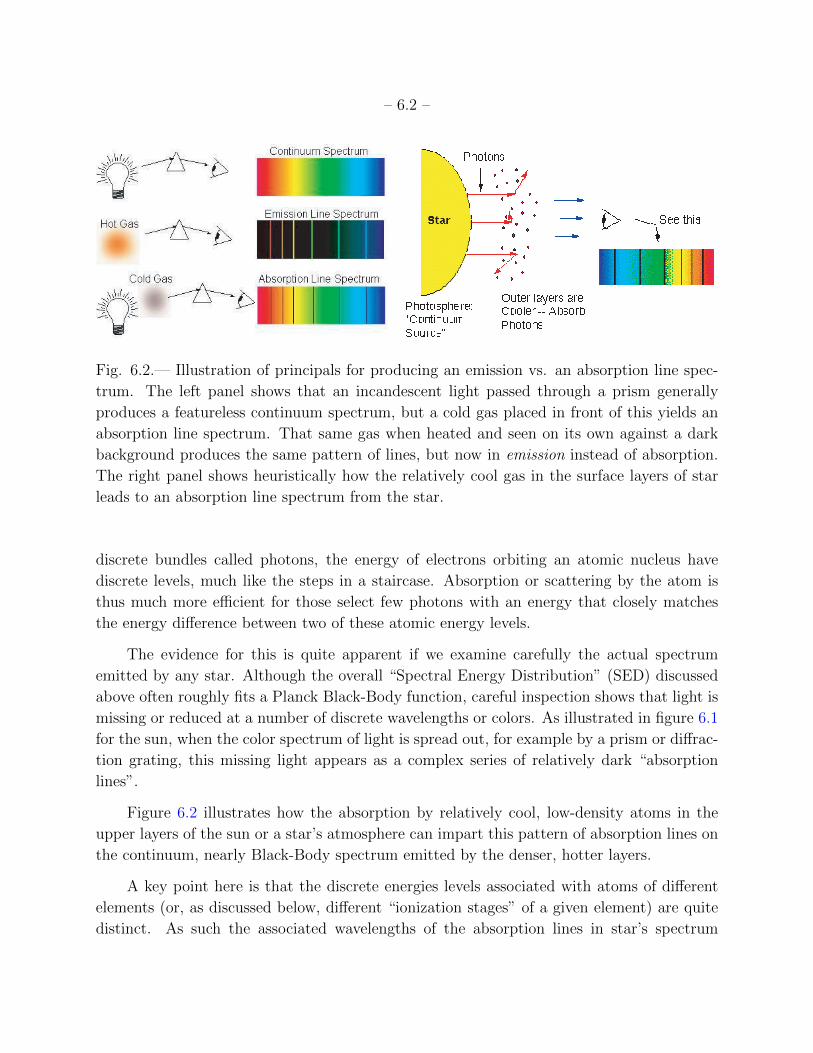
Fig. 6.2.— Illustration of principals for producing an emission vs. an absorption line spec-
trum. The left panel shows that an incandescent light passed through a prism generally
produces a featureless continuum spectrum, but a cold gas placed in front of this yields an
absorption line spectrum. That same gas when heated and seen on its own against a dark
background produces the same pattern of lines, but now in emission instead of absorption.
The right panel shows heuristically how the relatively cool gas in the surface layers of star
leads to an absorption line spectrum from the star.
discrete bundles called photons, the energy of electrons orbiting an atomic nucleus have
discrete levels, much like the steps in a staircase. Absorption or scattering by the atom is
thus much more efficient for those select few photons with an energy that closely matches
the energy difference between two of these atomic energy levels.
The evidence for this is quite apparent if we examine carefully the actual spectrum
emitted by any star. Although the overall “Spectral Energy Distribution” (SED) discussed
above often roughly fits a Planck Black-Body function, careful inspection shows that light is
missing or reduced at a number of discrete wavelengths or colors. As illustrated in figure 6.1
for the sun, when the color spectrum of light is spread out, for example by a prism or diffrac-
tion grating, this missing light appears as a complex series of relatively dark “absorption
lines”.
Figure 6.2 illustrates how the absorption by relatively cool, low-density atoms in the
upper layers of the sun or a star’s atmosphere can impart this pattern of absorption lines on
the continuum, nearly Black-Body spectrum emitted by the denser, hotter layers.
A key point here is that the discrete energies levels associated with atoms of different
elements (or, as discussed below, different “ionization stages” of a given element) are quite
distinct. As such the associated wavelengths of the absorption lines in star’s spectrum
– 6.3 –
provide a direct fingerprint – perhaps even more akin to a supermarket “bar code” – for the
presence of that element in the star’s atmosphere. The code “key” can come from laboratory
measurement of the line-spectrum from known samples of atoms and ions, or, as discussed in
§A, from theoretical models of the atomic energy levels using modern principles of quantum
physics.
HH
HeHe
LiLiBeBe
BB
CC
NN
OO
FF
NeNe
NaNa
MgMg
AlAl
SiSi
PP
SS
ClCl
ArAr
KK
CaCa
ScSc
TiTi
VV
CrCrMnMn
FeFe
CoCo
NiNi
CuCu
ZnZn
GaGa
GeGe
RbRbSrSr
YY
ZrZr
NbNbMoMoRuRuRhRhPdPdAgAg
CdCdInInSnSn
SbSb
CsCsBaBa
LaLaCeCe
PrPr
NdNd
SmSmEuEu
GdGd
TbTb
DyDyErEr
TmTm
YbYbLuLuHfHf
WW
ReRe
OsOsIrIr
PtPt
AuAu
HgHg
TlTl
PbPbBiBi
ThTh
UU
20 40 60 80
108
106
104
0.01
1
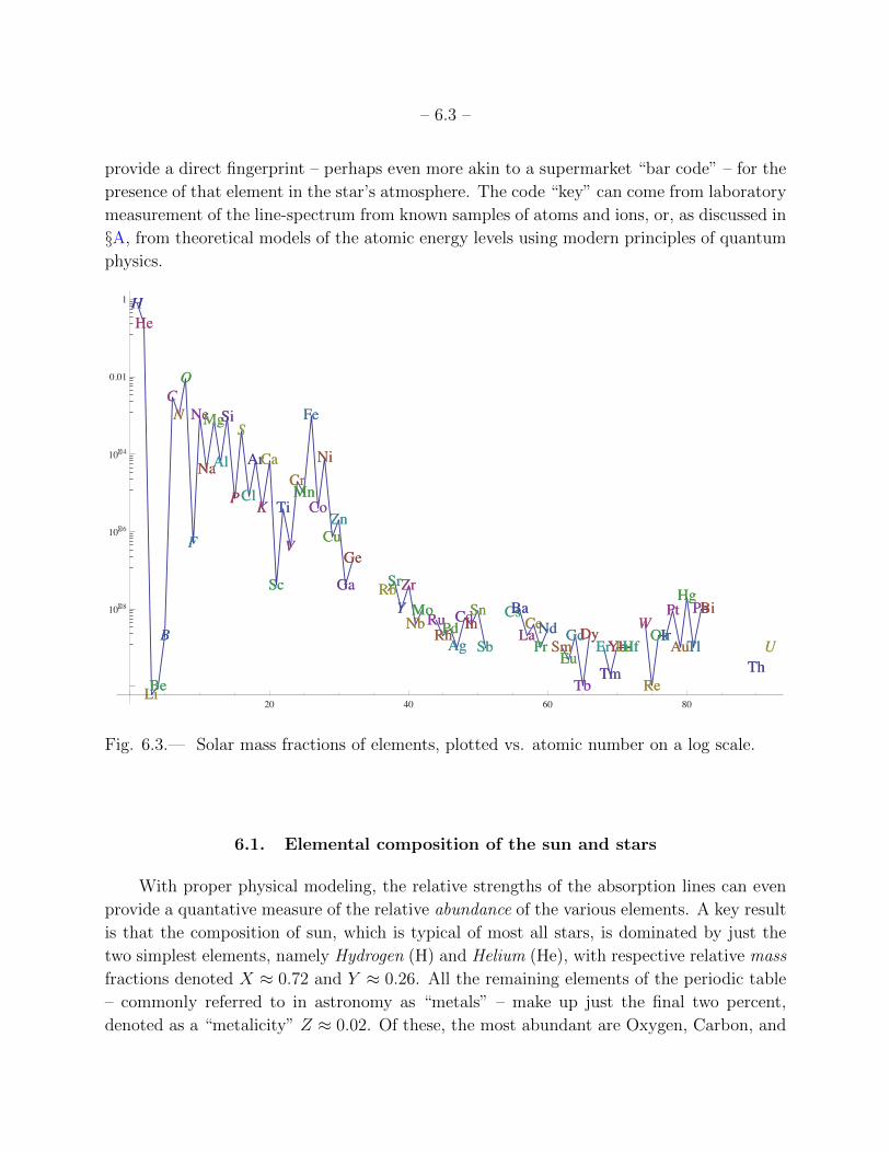
Fig. 6.3.— Solar mass fractions of elements, plotted vs. atomic number on a log scale.
6.1. Elemental composition of the sun and stars
With proper physical modeling, the relative strengths of the absorption lines can even
provide a quantative measure of the relative abundance of the various elements. A key result
is that the composition of sun, which is typical of most all stars, is dominated by just the
two simplest elements, namely Hydrogen (H) and Helium (He), with respective relative mass
fractions denoted X ≈ 0.72 and Y ≈ 0.26. All the remaining elements of the periodic table
– commonly referred to in astronomy as “metals” – make up just the final two percent,
denoted as a “metalicity” Z ≈ 0.02. Of these, the most abundant are Oxygen, Carbon, and
– 6.4 –
Iron, with respective mass fractions of 0.009, 0.003, and 0.001. Figure 6.3 gives a log plot of
the solar mass fraction vs. atomic number.
Like all the planets in our solar system, the Earth formed out of the same material that
makes up the sun. But its relatively weak gravity has allowed a lot of the light elements like
Hydrogen and Helium to escape into space, leaving behind the heavier elements that make
up our world, and us. Indeed, once the H and He are removed, the relative abundances of
all these heavier elements are roughly the same on the earth as in the sun!
6.2. Stellar spectral type: ionization abundances as temperature diagnostic
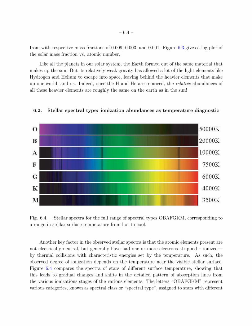
Fig. 6.4.— Stellar spectra for the full range of spectral types OBAFGKM, corresponding to
a range in stellar surface temperature from hot to cool.
Another key factor in the observed stellar spectra is that the atomic elements present are
not electrically neutral, but generally have had one or more electrons stripped – ionized—
by thermal collisions with characteristic energies set by the temperature. As such, the
observed degree of ionization depends on the temperature near the visible stellar surface.
Figure 6.4 compares the spectra of stars of different surface temperature, showing that
this leads to gradual changes and shifts in the detailed pattern of absorption lines from
the various ionizations stages of the various elements. The letters “OBAFGKM” represent
various categories, known as spectral class or “spectral type”, assigned to stars with different
– 6.5 –
spectral patterns. It turns out that type O is the hottest, with temperatures about 50,000 K,
while M is the coolest7 with temperatures of about 3500 K. The sequence is often remembered
through the mnemonic8 “Oh, Be A Fine Gal/Guy Kiss Me”. In keeping with its status as a
kind of average star, the sun has spectral type G, just at bit hotter than the type F in the
middle of the sequence.
In addition to the spectral classes OBAFGKM that depend on surface temperature T ,
spectra can also be organized in terms of luminosity classes, conventionally denoted though
Roman numerals I for the biggest, brightest “supergiant” stars, to V for smaller, dimmer
“dwarf” stars; in between, there are luminosity classes II (bright giants), III (giants), and
IV (sub-giants).
In this two-parameter scheme, the sun is classified as a G2V star.
Finally, in addition to giving information on the temperature, chemical composition, and
other conditions of a star’s atmosphere, these absorption lines provide convenient “markers”
in the star’s spectrum. As discussed in §9.2, this makes it possible to track small changes in
the wavelength of lines that arise from the so-called Doppler effect as a star moves toward
or away from us.
In summary, the appearance of absorption lines in stellar spectra provides a real treasure
trove of clues to the physical properties of stars.
6.3. Hertzsprung-Russell (H-R) diagram
A key diagnostic of stellar populations comes from the Hertzsprung-Russel (H-R) dia-
gram, illustrated by the left panel of figure 6.5. Observationally, it relates (absolute) magni-
tude (or luminosity class) on the y-axis, to color or spectral type on the x-axis; physically, it
relates luminosity to temperature. For stars in the solar neighborhood with parallaxes mea-
sured by the Hipparchus astrometry satellite, one can readily use the associated distance to
convert observed apparent magnitudes to absolute magnitudes and luminosities. The right
panel of figure 6.5 shows the H-R diagram for these stars, plotting their known luminosities
7In recent years, it has become possible to detect even cooler “Brown dwarf” stars, with spectral classes
LTY, extending down to temperatures as low as 1000 K. Brown dwarf stars have too low a mass (< 0.08M)
to force hydrogen fusion in their interior (see §16.3). They represent a link to gas giant planets like Jupiter
(for which MJ ≈ 0.001M).
8A student on one of my exams once offered an alternative mnemonic: “Oh Boy, Another F’s Gonna Kill
Me”.
– 6.6 –
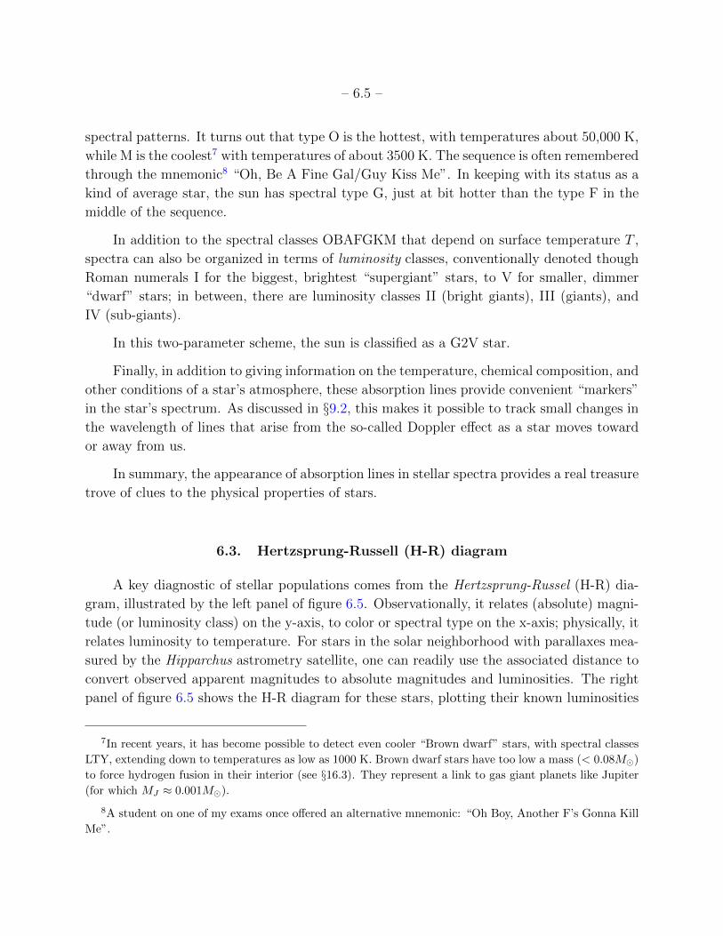
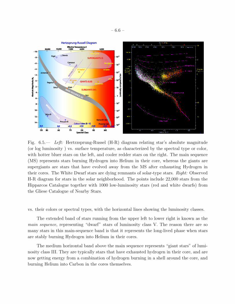
Fig. 6.5.— Left: Hertrzsprung-Russel (H-R) diagram relating star’s absolute magnitude
(or log luminosity ) vs. surface temperature, as characterized by the spectral type or color,
with hotter bluer stars on the left, and cooler redder stars on the right. The main sequence
(MS) represents stars burning Hydrogen into Helium in their core, whereas the giants are
supergiants are stars that have evolved away from the MS after exhausting Hydrogen in
their cores. The White Dwarf stars are dying remnants of solar-type stars. Right: Observed
H-R diagram for stars in the solar neighborhood. The points include 22,000 stars from the
Hipparcos Catalogue together with 1000 low-luminosity stars (red and white dwarfs) from
the Gliese Catalogue of Nearby Stars.
vs. their colors or spectral types, with the horizontal lines showing the luminosity classes.
The extended band of stars running from the upper left to lower right is known as the
main sequence, representing “dwarf” stars of luminosity class V. The reason there are so
many stars in this main-sequence band is that it represents the long-lived phase when stars
are stably burning Hydrogen into Helium in their cores.
The medium horizontal band above the main sequence represents “giant stars” of lumi-
nosity class III. They are typically stars that have exhausted hydrogen in their core, and are
now getting energy from a combination of hydrogen burning in a shell around the core, and
burning Helium into Carbon in the cores themselves.
– 6.7 –
The relative lack here of still more luminous supergiant stars of luminosity class I stems
from both the relative rarity of stars with sufficiently high mass to become this luminous,
coupled with the fact that such luminous stars only live for a very short time. As such,
there are only a few such massive, luminous stars in the solar neighborhood. Studying them
requires broader surveys extending to larger distances that encompass a greater fraction of
our galaxy.
The stars in the band below the main sequence are called white dwarfs; they represent
the slowly cooling remnant cores of low-mass stars like the sun.
This association between position on the H-R diagram, and stellar parameters and evo-
lutionary status, represents a key link between the observable properties of light emitted
from the stellar surface and the physical properties associated with the stellar interior. Un-
derstanding this link through examination of stellar structure and evolution will constitute
the major thrust of our studies of stellar interiors in part II of these notes.
But before we can do that, we need to consider ways that we can empirically determine
the two key parameters differentiating the various kinds of stars on this H-R diagram, namely
mass and age.
6.4. Questions and Exercises
Quick Question 1: On the H-R diagram, where do we find stars that are: a.)
Hot and luminous? b.) Cool and luminous? c.) Cool and Dim? d.) Hot and
Dim?
Which of these are known as: 1.) White Dwarfs? 2.) Red Giants? 3.) Blue
supergiants? 4.) Red dwarfs?

– 7.1 –
7. Surface Gravity and Escape/Orbital Speed
So far we’ve been able to finds ways to estimate the first five stellar parameters on our
list – distance, luminosity, temperature, radius, and elemental composition. Moreover, we’ve
done this with just a few, relatively simple measurements – parallax, apparent magnitude,
color, and spectral line patterns. But along the way we’ve had to learn to exploit some
key geometric principles and physical laws – angular-size/parallax, inverse-square law, and
Planck’s, Wien’s and the Stefan-Boltzman laws of blackbody radiation.
So what of the next item on the list, namely stellar mass?? Mass is clearly a physically
important parameter for a star, since for example it will help determine the strength of the
gravity that tries to pull the star’s matter together. To lay the groundwork for discussing
one basic way we can determine mass (from orbits of stars in stellar binaries), let’s first
review the Newton’s law of gravitation and show how this sets such key quantities like the
surface gravity, and the speeds required for material to escape or orbit the star.
7.1. Newton’s law of gravitation and stellar surface gravity
On Earth, an object of mass m has a weight given by
Fgrav = mge , (7.1)
where the acceleration of gravity on Earth is ge = 980 cm/s2 = 9.8m/s2. But this comes
from Newtons’s law of gravity, which states that for two point masses m and M separated
by a distance r, the attractive gravitational force between them is given by
Fgrav =GMm
r2, (7.2)
where Newton’s constant of gravity is G = 6.7× 10⁻⁸cm3/g/s2. Remarkably, when applied
to spherical bodies of mass M and finite radius R, the same formula works for all distances
r ≥ R at or outside the surface!9 Thus, we see that the acceleration of gravity at the surface
of the Earth is just given by the mass and radius of the Earth through
ge =GMe
R2e
. (7.3)
9Even more remarkably, even if we are inside the radius, r < R, then we can still use Newton’s law if we
just count that part of the total mass that is inside r, i.e. Mr, and completely ignore all the mass that is
above r.
– 7.2 –
Similarly for stars, the surface gravity is given by the stellar mass M and radius R. In the
case of the Sun, this gives g = 2.6 × 104cm/s2 ≈ 27 ge. Thus, if you could stand on the
surface of the Sun, your “weight” would be about 27 times what it is on Earth.
For other stars, gravities can vary over a quite wide range, largely because of the wide
range in size. For example, when the Sun get’s near the end of its life about 5 billion years
from now, it will swell up to more than 100 times its current radius, becoming what’s known
as a “Red Giant”. Stars we see now that happen to be in this Red Giant phase thus tend
to have quite low gravity, about a fraction 1/10,000 that of the Sun.
Largely because of this very low gravity, much of the outer envelope of such Red Giant
stars will actually be lost to space (forming, as we shall see, quite beautiful nebulae). When
this happens to the Sun, what’s left behind will be just the hot stellar core, a so-called “white
dwarf”, with about 2/3 the mass of the current Sun, but with a radius only about that of
the Earth, i.e. R ≈ Re ≈ 7 × 10³ km ≈ 0.01R. The surface gravities of white dwarfs are
thus typically 10, 000 times higher than the current Sun.
For “neutron stars”, which are the remnants of stars a bit more massive than the Sun, the
radius is just about 10 km, more than another factor 500 smaller than white dwarfs. This
implies surface gravities another 5-6 orders of magnitude higher than even white dwarfs.
(Imagine what you’d weigh then on the surface of a neutron star!)
Since stellar gravities vary over such a large range, it is customary to quote them in
terms of the log of the gravity, log g, using CGS units. We thus have gravities ranging
from log g ≈ 0 for Red Giants, to log g ≈ 4 for normal stars like the Sun, to log g ≈ 8 for
white dwarfs, to log g ≈ 13 for neutron stars. Since the Earth’s gravity has log ge ≈ 3, the
difference of log g from 3 is the number of order of magnitudes more/less that you’d weigh
on that surface. For example, for neutron stars the difference from Earth is 10, implying
you’d weigh 1010, or ten billion, times more on a neutron star! On the other hand, on a Red
Giant, your weight would be about 1000 times less than on Earth.
7.2. Surface escape speed Vesc
Another measure of the strength of a gravitational field is through the surface escape
speed,
Vesc =
√2GM
R. (7.4)
A object of mass m launched with this speed has a kinetic energy mV 2esc/2 = GMm/R. This
just equals the work needed to lift that object from the surface radius R to escape at a large
– 7.3 –
radius r →∞,
W =
∫ ∞R
GMm
r2dr =
GMm
R. (7.5)
Thus if one could throw a ball (or launch a rocket!) with this speed outward from a body’s
surface radiusR, then10 by conservation of total energy, that object would reach an arbitrarily
large distance from the star, with however a vanishingly small final speed.
For the earth, the escape speed is about 25,000 mph, or 11.2 km/s. By comparison, for
the moon, it is just 2.4 km/s, which is one reason the Apollo astronauts could use a much
smaller rocket to get back from the moon, than they used to get there in the first place.
However, escaping from the surface of the sun (and most any star), is much harder, requiring
an escape speed of 618 km/s.
7.3. Speed for circular orbit
Let us next compare this escape speed with the speed needed for an object to maintain a
circular orbit at some radius r from the center a gravitating body of mass M . For an orbiting
body of mass m, we require that the gravitational force be balanced by the centrifugal force
from moving along the circle of radius r,
GMm
r2=mV 2
orb
r, (7.6)
which solves to
Vorb(r) =
√GM
r. (7.7)
Note in particular that the orbital speed very near the stellar surface, r ≈ R, is given
by Vorb(R) = Vesc/√
2. Thus the speed of satellites in low-earth-orbit (LEO) is about
17,700 mph, or 7.9 km/s.
Of course, orbits can also be maintained at any radius above the surface radius, r > R,
and eqn. (7.7) shows that in this case, the speed needed declines as 1/√r. Thus, for example,
the orbital speed of the earth around the sun is about 30 km/s, a factor of√R/au =√
1/215 = 0.0046 smaller than the orbital speed near the sun’s surface, Vorb, = 434 km/s.
10neglecting forces other than gravity, like the drag from an atmosphere
– 7.4 –
7.4. Virial Theorum for bound orbits
If we define the gravitational energy to be zero far from a star, then for an object of
mass m at a radius r from a star of mass M , we can write the gravitational binding energy
U as the negative of the escape energy,
U(r) = −GMm
r. (7.8)
If this same object is in orbit at this radius r, then the kinetic energy of the orbit is
T (r) =mV 2
orb
2= +
GMm
2r= −U(r)
2, (7.9)
where the second equation uses eqn. (7.7) for the orbital speed Vorb(r). We can then write
the total energy as
E(r) ≡ T (r) + U(r) = −T (r) =U(r)
2. (7.10)
This fact that the total energy E just equals half the gravitational binding energy U is an
example of what is known as the Virial Theorum. It is applicable broadly to most any stably
bound gravitational system. For example, if we recognize that the thermal energy inside a
star as a kind of kinetic energy, it even applies to stars, in which the internal gas pressure
balances the star’s own self gravity. This is discussed further in §8.2 and the part II notes
on stellar structure.
7.5. Questions and Exercises
Quick Question 1: In CGS units, the sun has log g ≈ 4.44. Compute the
log g for stars with:
a. M = 10M and R = 10Rb. M = 1M and R = 100Rc. M = 1M and R = 0.01R
Quick Question 2:
The sun has an escape speed of Ve = 618 km/s. Compute the escape speed
Ve of the stars in parts a-c of QQ1.
Quick Question 3:
The earth has an orbital speed of Ve = 2πau/yr = 30 km/s. Compute the
orbital speed Vorb (in km/s) of a body at the following distances from the stars
with the quoted masses:
– 7.5 –
a. M = 10M and d = 10 au.
b. M = 1M and d = 100 au.
c. M = 1M and d = 0.01 au.
Exercise 1:
a. During a solar eclipse, the moon just barely covers the visible disk of the
sun. What does this tell you about the relative angular size of the sun and moon?
b. Given that the moon is at a distance of 0.0024 au, what then is the ratio
of the physical size of the moon vs. sun?
c. Compared to earth, the sun and moon have gravities of respectively 27geand ge/6. Using this and your answer above, what is the ratio of the mass of the
moon to that of the sun?
d. Using the above, plus known values for Newton’s constant G, earth’s
gravity ge = 9.8 m/s2, and the solar radius R = 700, 000 km, compute the
masses of the sun and moon in kg.
Exercise 2:
a. What is the ratio of the energy needed to escape the moon vs. the earth?
What’s the ratio for the sun vs. the earth?
b. What is the escape speed (in km/s) from a star with: (1) M = 10M and
R = 10R; (2) M = 1M and R = 100R; (3) M = 1M and R = 0.01R?
c. To what radius (in km) would you have to shrink the sun to make its
escape speed equal to the speed of light c?
Exercise 3:
a. What is the ratio of the energy needed to escape the the earth vs. that
needed to reach LEO?
b. What is the orbital speed (in km/s) of a planet that orbits at a distance a
from a star with mass M , given: (1) M = 10M and a = 10 au; (2) M = 1Mand a = 100, au; (3) M = 1M and a = 0.01 au?

– 8.1 –
8. Stellar Ages and Lifetimes
In our list of basic stellar properties, let us next consider stellar age. Just how old
are stars like the sun? What provides the energy that keeps them shining? And what will
happen to them as they exhaust various available energy sources?
8.1. Shortness of chemical burning timescale for sun and stars
When 19th century scientists pondered the possible energy sources for the sun, some
first considered whether this could come from the kind of chemical reactions (e.g., from
fossil fuels like coal, oil, natural gas, etc.) that power human activities on earth. But such
chemical reactions involve transitions of electrons among various bound states of atoms, and,
as discussed below (§A) for the Bohr model of the Hydrogen, the scale of energy release in
such transitions is limited to something on the order of an electron volt (eV). In contrast,
the rest-mass energy of the protons and neutrons that make up the mass is about 1 Gev,
or 109 times higher. With the associated mass-energy efficiency of ε ∼ 10−9, we can readily
estimate a timescale for maintaining the solar luminosity from chemical reactions,
tchem = εMc
2
L= ε 4.5× 10²⁰ s = ε 1.5× 10¹³ yr ≈ 15, 000 yr . (8.1)
Even in the 19th century, it was clear, e.g. from geological processes like erosion, that the
earth – and so presumably also the sun – had to be much older than this.
8.2. Kelvin-Helmholtz timescale for gravitational contraction
So let us instead consider whether, instead of chemical reactions, gravitational contrac-
tion might provide the energy source to power the sun and other stars. As a star undergoes a
contraction in radius, its gravitational binding becomes stronger, with a deeper gravitational
potential energy, yielding an energy release set by the negative of the change in gravitational
potential (−dU >0). If the contraction is gradual enough that the star roughly maintains dy-
namical equilibrium, then just half of the gravitational energy released goes into heating up
the star11, leaving the other half available to power the radiative luminosity, L = −12dU/dt.
For a star of observed luminosity L and present-day gravitational binding energy U , we can
11This is another example of the Virial theorem for gravitationally bound systems, as discussed in 7.4.
– 8.2 –
thus define a characteristic gravitational contraction lifetime,
tgrav = −1
2
U
L≡ tKH (8.2)
where the subscript “KH” refers to Kelvin and Helmholtz, the names of the two scientists
credited with first identifying this as an important timescale. To estimate a value for the
gravitational binding energy, let us consider the example for the sun under the somewhat
artificial assumption that it has a uniform, constant density, given by its mass over volume,
ρ = M/(4πR3/3). Since the gravity at any radius r depends only on the mass m = ρ4πr3/3
inside that radius, the total gravitational binding energy of the sun is given by integrating
the associated local gravitational potential −Gm/r over all differential mass shells dm,
− U =
∫ M
0
Gm
rdm =
16π2
3Gρ2
∫ R
0
r4 dr =3
5
GM2
R, (8.3)
Applying this in eqn. (8.2), we find for the “Kelvin-Helmholtz” time of the sun,
tKH ≈3
10
GM2
RL≈ 30 Myr . (8.4)
Although substantially longer than the chemical burning timescale (8.1), this is still much
shorter than the geologically inferred minimum age of the earth, which is several Billion
years.
8.3. Nuclear burning timescale
We now realize, of course, that the ages and lifetimes of stars like the sun are set by a
much longer nuclear burning timescale. When four hydrogen nuclei are fused into a helium
nucleus, the helium mass is about 0.7% lower than the original four hydrogen. For nuclear
fusion the above-defined mass-energy burning efficiency is thus now εnuc ≈ 0.007. But in a
typical main sequence star, only some core fraction f ≈ 1/10 of the stellar mass is hot enough
to allow hydrogen fusion. Applying this we thus find for the nuclear burning timescale
tnuc = εnuc fMc2
L≈ 10 Gyr
M/ML/L
, (8.5)
where Gyr≡ 109 yr, i.e., a billion years, or a “Giga-year”.
We thus see that the sun can live for about 10 Gyr by burning Hydrogen into Helium
– 8.3 –
in its core. It’s present age of 4.7 Gyr12 thus puts it roughly half way through this hydrogen-
burning phase, with about 5 Gyr to go before it runs out of H in its core.
8.4. Age of stellar clusters from main-sequence turnoff point
As discussed below (see §10.4 and eqn. 10.11), observations of stellar binary systems
indicate that the luminosities of main-sequence stars scale with a high power of the stellar
mass – roughly L ∼ M3. In the present context, this implies that high-mass stars should
have much shorter lifetimes than low-mass stars.
If we make the reasonable assumption that the same fixed fraction (f ≈ 0.1) of the total
hydrogen mass of any star is available for nuclear burning into helium in its stellar core, then
the fuel available scales with the mass, while the burning rate depends on the luminosity.
Normalized to the sun, the main-sequence lifetime thus scales as
tms = tms,M/ML/L
≈ 10 Gyr
(MM
)2
. (8.6)
The most massive stars, of order 100M, and thus with luminosities of order 106L, have
main-sequence lifetimes of only about about 1 Myr, much shorter the multi-Gyr timescale
for solar-mass stars.
This strong scaling of lifetime with mass can be vividly illustration by plotting the H-R
diagram of stellar clusters. The H-R diagram plotted in figure 6.5 is for volume-limited
sample near the sun, consisting of stars of a wide range of ages, distances, and perhaps even
chemical composition. But stars often appear clusters, all roughly at the same distance, and,
since they likely formed over a relatively short time span out of the same interstellar cloud,
all with roughly the same age and chemical composition. Using eqn. (8.6) together with the
the L ∼M3 relation, the age of a stellar cluster can be inferred from its H-R diagram simply
by measuring the luminosity Lto of stars at the “turn-off” point from the main sequence,
tcluster ≈ 10 Gyr
(LLto
)2/3
. (8.7)
The left panel of figure 8.1 plots an actual H-R diagram for the globular cluster M55.
Note that all the stars in the upper left of the main sequence have evolved to a vertical
12As inferred, e.g., from radioactive dating of the oldest meteorites.
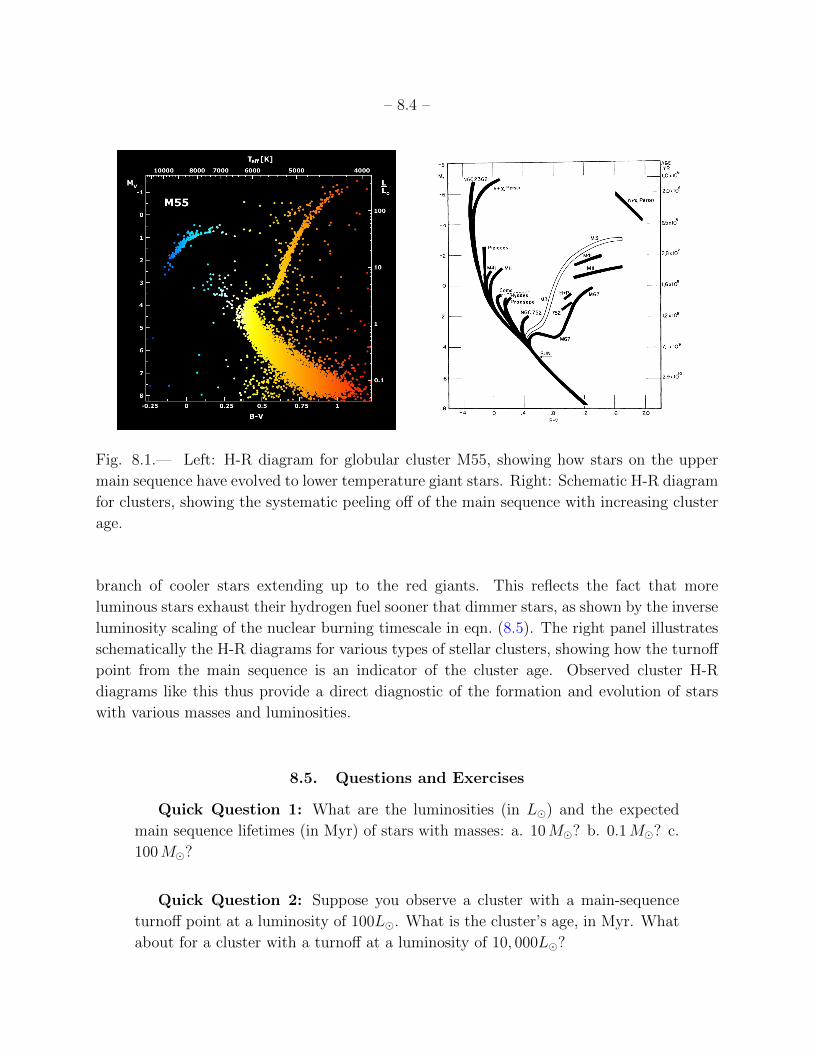
– 8.4 –
Fig. 8.1.— Left: H-R diagram for globular cluster M55, showing how stars on the upper
main sequence have evolved to lower temperature giant stars. Right: Schematic H-R diagram
for clusters, showing the systematic peeling off of the main sequence with increasing cluster
age.
branch of cooler stars extending up to the red giants. This reflects the fact that more
luminous stars exhaust their hydrogen fuel sooner that dimmer stars, as shown by the inverse
luminosity scaling of the nuclear burning timescale in eqn. (8.5). The right panel illustrates
schematically the H-R diagrams for various types of stellar clusters, showing how the turnoff
point from the main sequence is an indicator of the cluster age. Observed cluster H-R
diagrams like this thus provide a direct diagnostic of the formation and evolution of stars
with various masses and luminosities.
8.5. Questions and Exercises
Quick Question 1: What are the luminosities (in L) and the expected
main sequence lifetimes (in Myr) of stars with masses: a. 10M? b. 0.1M? c.
100M?
Quick Question 2: Suppose you observe a cluster with a main-sequence
turnoff point at a luminosity of 100L. What is the cluster’s age, in Myr. What
about for a cluster with a turnoff at a luminosity of 10, 000L?
– 8.5 –
Exercise 1: A cluster has a main-sequence turnoff at a spectral type G2,
corresponding to stars of apparent magnitude m = +10.
(a) About what is the luminosity, in L, of the stars at the turnoff point?
(b) About what is the age (in Gyr) of the cluster?
(c) About what is the distance (in pc) of the cluster?
Exercise 2: Confirm the integration result in eqn. (8.3).
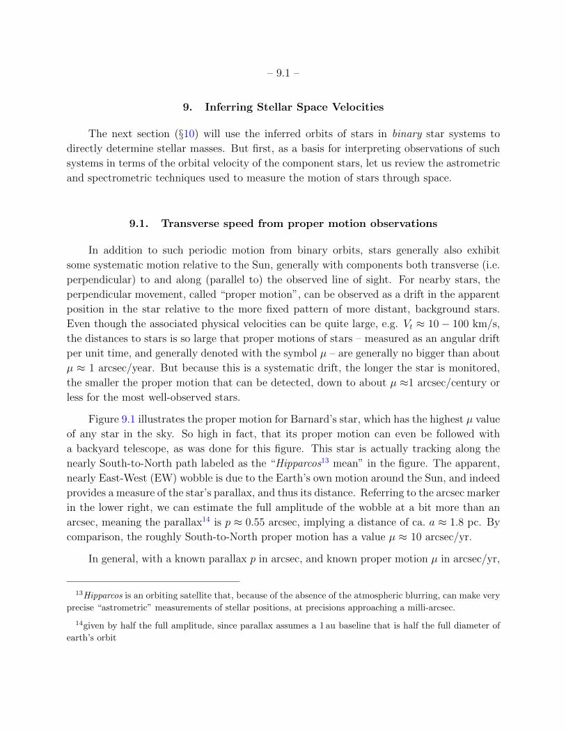
– 9.1 –
9. Inferring Stellar Space Velocities
The next section (§10) will use the inferred orbits of stars in binary star systems to
directly determine stellar masses. But first, as a basis for interpreting observations of such
systems in terms of the orbital velocity of the component stars, let us review the astrometric
and spectrometric techniques used to measure the motion of stars through space.
9.1. Transverse speed from proper motion observations
In addition to such periodic motion from binary orbits, stars generally also exhibit
some systematic motion relative to the Sun, generally with components both transverse (i.e.
perpendicular) to and along (parallel to) the observed line of sight. For nearby stars, the
perpendicular movement, called “proper motion”, can be observed as a drift in the apparent
position in the star relative to the more fixed pattern of more distant, background stars.
Even though the associated physical velocities can be quite large, e.g. Vt ≈ 10− 100 km/s,
the distances to stars is so large that proper motions of stars – measured as an angular drift
per unit time, and generally denoted with the symbol µ – are generally no bigger than about
µ ≈ 1 arcsec/year. But because this is a systematic drift, the longer the star is monitored,
the smaller the proper motion that can be detected, down to about µ ≈1 arcsec/century or
less for the most well-observed stars.
Figure 9.1 illustrates the proper motion for Barnard’s star, which has the highest µ value
of any star in the sky. So high in fact, that its proper motion can even be followed with
a backyard telescope, as was done for this figure. This star is actually tracking along the
nearly South-to-North path labeled as the “Hipparcos13 mean” in the figure. The apparent,
nearly East-West (EW) wobble is due to the Earth’s own motion around the Sun, and indeed
provides a measure of the star’s parallax, and thus its distance. Referring to the arcsec marker
in the lower right, we can estimate the full amplitude of the wobble at a bit more than an
arcsec, meaning the parallax14 is p ≈ 0.55 arcsec, implying a distance of ca. a ≈ 1.8 pc. By
comparison, the roughly South-to-North proper motion has a value µ ≈ 10 arcsec/yr.
In general, with a known parallax p in arcsec, and known proper motion µ in arcsec/yr,
13Hipparcos is an orbiting satellite that, because of the absence of the atmospheric blurring, can make very
precise “astrometric” measurements of stellar positions, at precisions approaching a milli-arcsec.
14given by half the full amplitude, since parallax assumes a 1 au baseline that is half the full diameter of
earth’s orbit
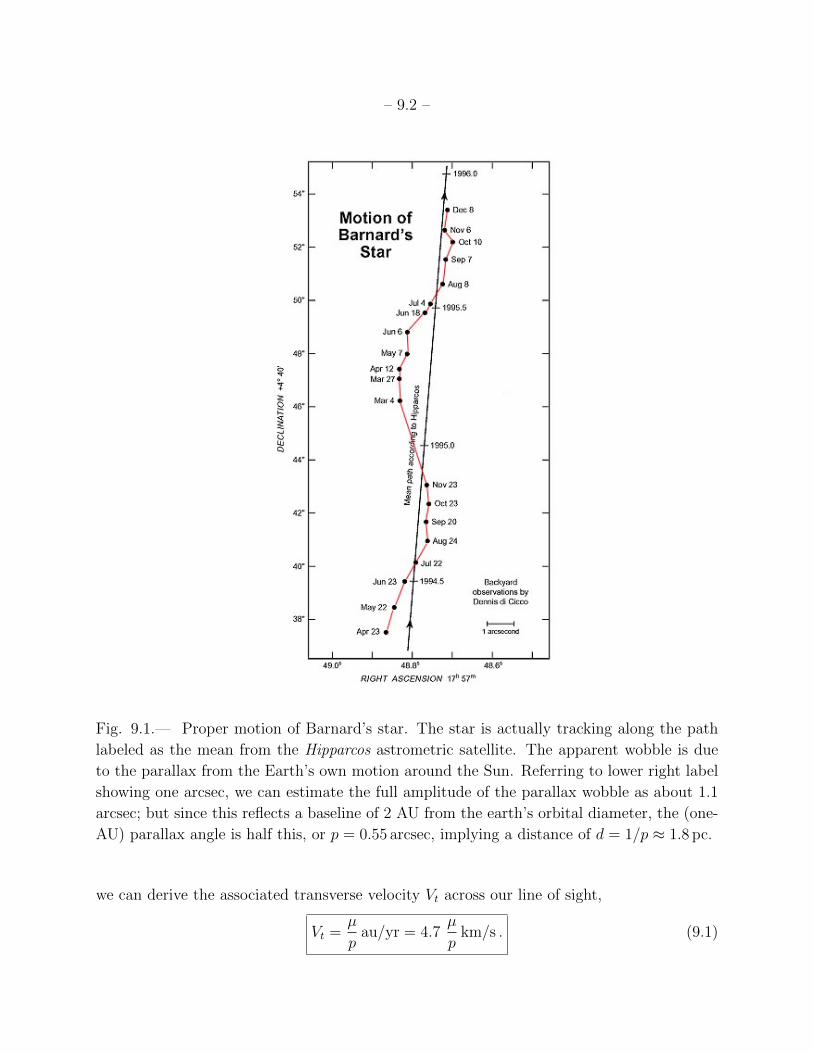
– 9.2 –
Fig. 9.1.— Proper motion of Barnard’s star. The star is actually tracking along the path
labeled as the mean from the Hipparcos astrometric satellite. The apparent wobble is due
to the parallax from the Earth’s own motion around the Sun. Referring to lower right label
showing one arcsec, we can estimate the full amplitude of the parallax wobble as about 1.1
arcsec; but since this reflects a baseline of 2 AU from the earth’s orbital diameter, the (one-
AU) parallax angle is half this, or p = 0.55 arcsec, implying a distance of d = 1/p ≈ 1.8 pc.
we can derive the associated transverse velocity Vt across our line of sight,
Vt =µ
pau/yr = 4.7
µ
pkm/s . (9.1)

– 9.3 –
For Barnard’s star this works out to give Vt ≈ 90 km/s, or about 3 times the earth’s orbital
speed around the sun. This among the fastest transverse speeds inferred among the nearby
stars.
9.2. Radial velocity from Doppler shift
We’ve seen how we can directly measure the transverse motion of relatively nearby,
fast-moving stars in terms of their proper motion. But how might we measure the radial
velocity component along our line of sight? The answer is: via the “Doppler effect”, wherein
such radial motion leads to an observed shift in the wavelength of the light.
To see how this effect comes about, we need only consider some regular signal with
period Po being emitted from a object moving at a speed Vr toward (Vr < 0) or away
(Vr > 0) from us. Let the signal travel at a speed Vs, where Vs = c for a light wave, but
might equally as well be speed of sound if we were to use that as an example. For clarity of
language, let us assume the object is moving away, with Vr > 0. Then after any given pulse
of the signal is emitted, the object moves a distance VrPo before emitting the next pulse.
Since the pulse still travels at the same speed, this implies it takes the second pulse an extra
time
∆P =VrPoVs
(9.2)
to reach us. Thus the period we observe is longer, P ′ = Po + ∆P .
For a wave, the wavelength is given by λ = PVs, implying then an associated stretch in
the observed wavelength
λ′ = P ′Vs = (Po + ∆P )Vs = (Vs + Vr)Po = λo + VrPo . (9.3)
where λo = PoVs is the rest wavelength. The associated relative stretch in wavelength is thus
just∆λ
λo≡ λ′ − λo
λo=
VrVs. (9.4)
For sound waves, this formula works in principle as long as Vr > −Vs. But if an object moves
toward us faster than sound (Vr < −Vs), then it can basically “overrun” the signal. This
leads to strongly compressed sound waves, called “shock waves”, which are the basic origin
of the sonic boom from a supersonic jet. For some nice animations of this, see
http://www.kettering.edu/∼drussell/Demos/doppler/doppler.html
There’s also a neat java applet at:
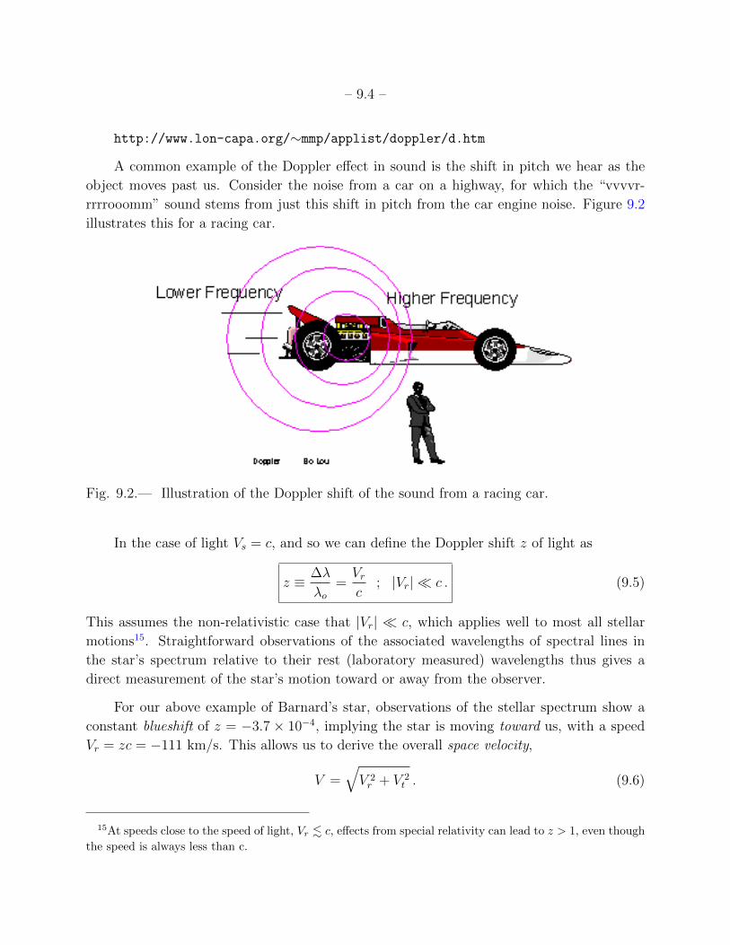
– 9.4 –
http://www.lon-capa.org/∼mmp/applist/doppler/d.htm
A common example of the Doppler effect in sound is the shift in pitch we hear as the
object moves past us. Consider the noise from a car on a highway, for which the “vvvvr-
rrrrooomm” sound stems from just this shift in pitch from the car engine noise. Figure 9.2
illustrates this for a racing car.
Fig. 9.2.— Illustration of the Doppler shift of the sound from a racing car.
In the case of light Vs = c, and so we can define the Doppler shift z of light as
z ≡ ∆λ
λo=Vrc
; |Vr| c . (9.5)
This assumes the non-relativistic case that |Vr| c, which applies well to most all stellar
motions15. Straightforward observations of the associated wavelengths of spectral lines in
the star’s spectrum relative to their rest (laboratory measured) wavelengths thus gives a
direct measurement of the star’s motion toward or away from the observer.
For our above example of Barnard’s star, observations of the stellar spectrum show a
constant blueshift of z = −3.7 × 10⁻⁴, implying the star is moving toward us, with a speed
Vr = zc = −111 km/s. This allows us to derive the overall space velocity,
V =√V 2r + V 2
t . (9.6)
15At speeds close to the speed of light, Vr . c, effects from special relativity can lead to z > 1, even though
the speed is always less than c.
– 9.5 –
For Barnard’s star, this gives V = 143 km/s, which again is one of the highest space velocities
among nearby stars. Mapping the space motion of nearby stars relative to the Sun provides
some initial clues about the kinematics of stars in our local region of the Milky Way galaxy.
9.3. Questions and Exercises
Quick Question 1: A star with parallax p = 0.02 arcsec is observed over 10
years to have shifted by 2 arcsec from its proper motion. Compute the star’s
tangential space velocity Vt, in km/s.
Quick Question 2: For the star in QQ#1, a line with rest wavelength λo =
600.00 nm is observed to be at a wavelength λ = 600.09 nm.
a. Is the star moving toward us or away from us?
b. What is the star’s Doppler shift z?
c. What is the star’s radial velocity Vr, in km/s?
d. What is the star’s total space velocity Vtot, in km/s?
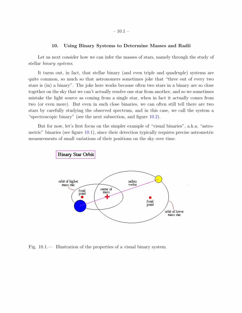
– 10.1 –
10. Using Binary Systems to Determine Masses and Radii
Let us next consider how we can infer the masses of stars, namely through the study of
stellar binary systems.
It turns out, in fact, that stellar binary (and even triple and quadruple) systems are
quite common, so much so that astronomers sometimes joke that “three out of every two
stars is (in) a binary”. The joke here works because often two stars in a binary are so close
together on the sky that we can’t actually resolve one star from another, and so we sometimes
mistake the light source as coming from a single star, when in fact it actually comes from
two (or even more). But even in such close binaries, we can often still tell there are two
stars by carefully studying the observed spectrum, and in this case, we call the system a
“spectroscopic binary” (see the next subsection, and figure 10.2).
But for now, let’s first focus on the simpler example of “visual binaries”, a.k.a. “astro-
metric” binaries (see figure 10.1), since their detection typically requires precise astrometric
measurements of small variations of their positions on the sky over time.
Fig. 10.1.— Illustration of the properties of a visual binary system.
– 10.2 –
10.1. Visual binaries
In visual binaries, monitoring of the stellar positions over years and even decades reveals
that the two stars are actually moving around each other, much as the Earth moves around
the Sun. Figure 10.1 illustrates the principles behind visual binaries. The time it takes the
stars to go around a full cycle, called the orbital period, can then be measured quite directly.
Then if we can convert the apparent angular separation into a physical distance apart – e.g.
if we know the distance to the system independently through a measured annual parallax for
the stars in the system – then we can use Kepler’s 3rd law of orbital motion (as generalized
by Newton) to measure the total mass of the two stars.
It’s actually quite easy to derive the full formula in the simple case of circular orbits
that lie in a plane perpendicular to our line of sight. For stars of mass M1 and M2 separated
by a physical distance a, Newton’s law of gravity gives the attractive force each star exerts
on the other,
Fg =GM1M2
a2. (10.1)
A key difference from the case of a satellite orbiting the earth, or a planet orbiting a star, is
that in binary stars, the masses can become comparable. In this case, each star (1,2) now
moves around the center of mass at a fixed distance a1 and a2, with their ratio given by
a2/a1 = M1/M2 and their sum by a1 + a2 = a. In terms of the full separation, the orbital
distance of, say, star 1 is thus given by
a1 = aM2
M1 +M2
. (10.2)
For the given period P , the associated orbital speeds for star 1 is is given by V1 = 2πa1/P .
For a stable, circular orbit, the outward centrifugal force on star 1,
Fc1 =M1V
21
a1
=4π2M1a1
P 2=
4π2a
P 2
M1M2
M1 +M2
, (10.3)
must balance the gravitational force from eqn. (10.1), yielding
GM1M2
a2=
4π2a
P 2
M1M2
M1 +M2
. (10.4)
This can be used to obtain the sum of the masses,
M1 +M2 =4π2
G
a3
P 2=a3au
P 2yr
M , (10.5)
where the latter equality shows that evaluating the distance in au and the period in years
gives the mass in units of the solar mass. For a visual binary in which we can actually see
– 10.3 –
both stars, we can separately measure the two orbital distances, yielding then the mass ratio
M2/M1 = a1/a2. The mass for, e.g., star 1 is thus given by
M1 =a3au
(1 + a1/a2)P 2yr
M . (10.6)
The mass for star 2 can likewise be obtained if we just swap subscripts 1 and 2.
Equations (10.5) and (10.6) are actually forms of Kepler’s 3rd law for planetary motion
around the Sun. Setting M1 = M and the planetary mass M2, we first note that for all
planets the mass is much smaller than for the Sun, M2/M1 = a1/a2 1, implying that the
Sun only slightly wobbles (mostly to the counter the pull of the most massive planet, namely
Jupiter), with the planets thus pretty much all orbiting around the Sun. If we thus ignore
M2 and plug in M1 = M in eqn. (10.5), we recover Kepler’s third law in (almost) the form
in which he expressed it,
P 2yr = a3
au . (10.7)
To be precise, Kepler showed that in general the orbits of the planets are actually ellipses,
but this same law applies in that case we if we replace the circular orbital distance a with
the “semi-major axis” of the ellipse. A circle is just a special case of an ellipse, with the
semi-major axis just equal to the radius.
In general, of course, real binary systems often have elliptical orbits, which, moreover,
lie in planes that are not always normal to the observer line of sight. These systems can still
be fully analyzed using the elliptical orbit form of Newton’s generalization of Kepler’s 3rd
law, as derived, e.g. in Ch. 4 of the Astro 45 notes by Bill Press:
http://www.lanl.gov/DLDSTP/ay45/ay45c4.pdf
Indeed, by watching the rate of movement of the stars along the projected orbit, the incli-
nation effect can even be disentangled from the ellipticity.
There are some useful java applets illustrating visual and spectroscopic binaries at:
http://csep10.phys.utk.edu/astr162/lect/binaries/visual.html
http://instruct1.cit.cornell.edu/courses/astro101/java/binary/binary.htm
10.2. Spectroscopic binaries
As noted, there are many stellar binary systems in which the angular separation between
the components is too close to readily resolve visually. However, if the orbital plane is not
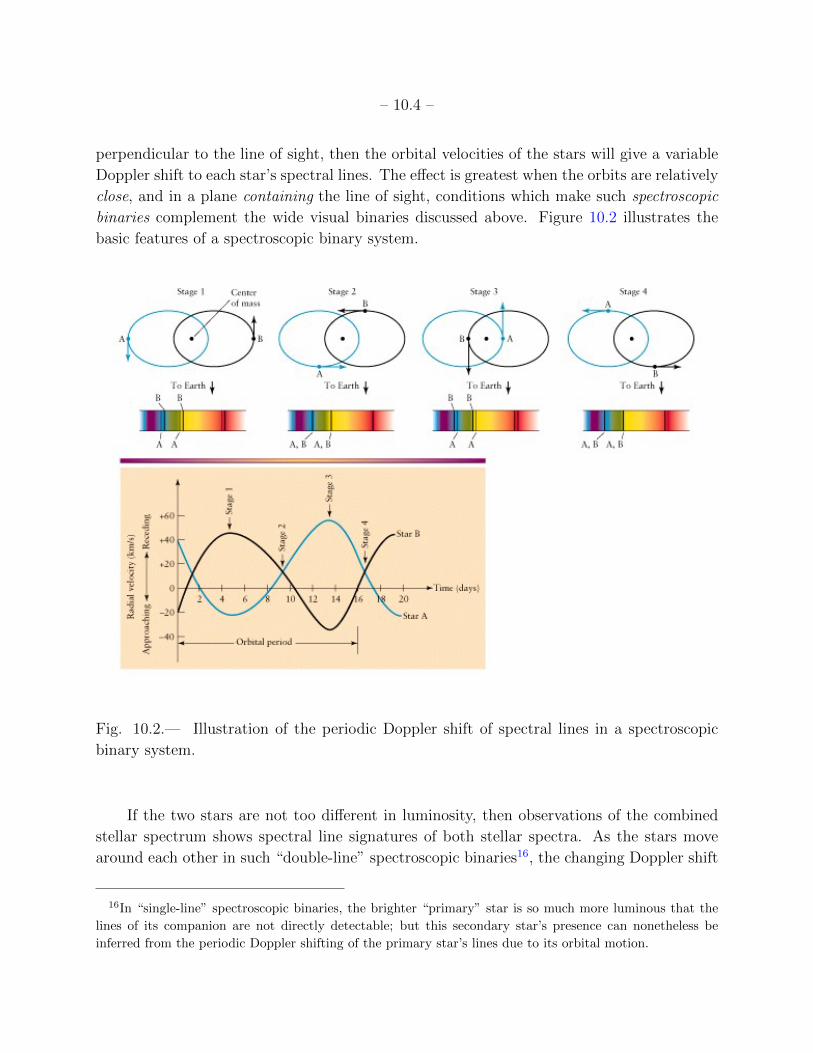
– 10.4 –
perpendicular to the line of sight, then the orbital velocities of the stars will give a variable
Doppler shift to each star’s spectral lines. The effect is greatest when the orbits are relatively
close, and in a plane containing the line of sight, conditions which make such spectroscopic
binaries complement the wide visual binaries discussed above. Figure 10.2 illustrates the
basic features of a spectroscopic binary system.
Fig. 10.2.— Illustration of the periodic Doppler shift of spectral lines in a spectroscopic
binary system.
If the two stars are not too different in luminosity, then observations of the combined
stellar spectrum shows spectral line signatures of both stellar spectra. As the stars move
around each other in such “double-line” spectroscopic binaries16, the changing Doppler shift
16In “single-line” spectroscopic binaries, the brighter “primary” star is so much more luminous that the
lines of its companion are not directly detectable; but this secondary star’s presence can nonetheless be
inferred from the periodic Doppler shifting of the primary star’s lines due to its orbital motion.
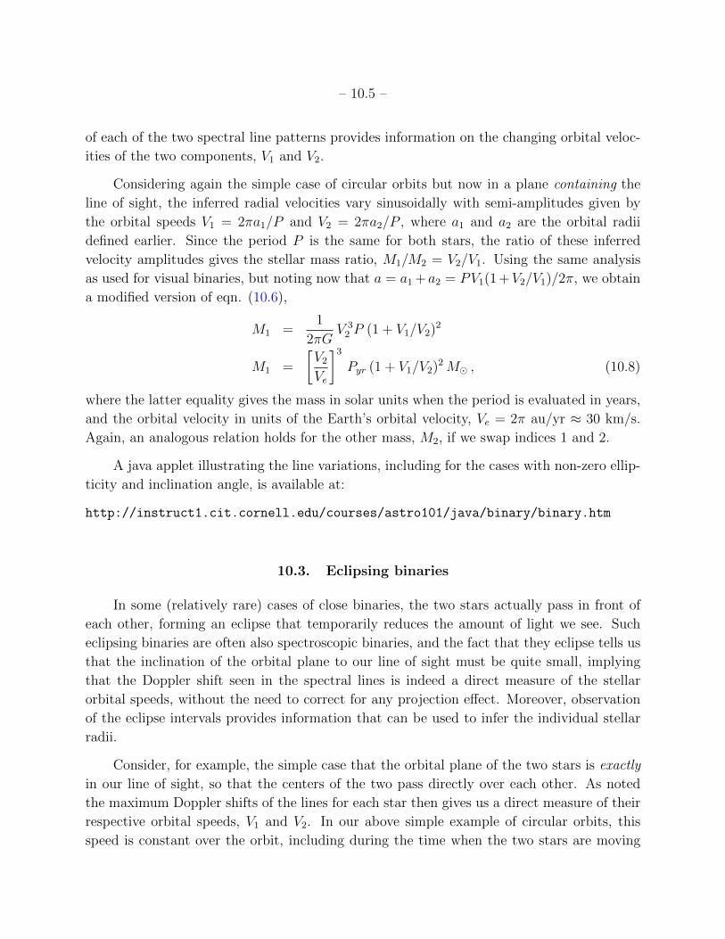
– 10.5 –
of each of the two spectral line patterns provides information on the changing orbital veloc-
ities of the two components, V1 and V2.
Considering again the simple case of circular orbits but now in a plane containing the
line of sight, the inferred radial velocities vary sinusoidally with semi-amplitudes given by
the orbital speeds V1 = 2πa1/P and V2 = 2πa2/P , where a1 and a2 are the orbital radii
defined earlier. Since the period P is the same for both stars, the ratio of these inferred
velocity amplitudes gives the stellar mass ratio, M1/M2 = V2/V1. Using the same analysis
as used for visual binaries, but noting now that a = a1 +a2 = PV1(1 +V2/V1)/2π, we obtain
a modified version of eqn. (10.6),
M1 =1
2πGV 3
2 P (1 + V1/V2)2
M1 =
[V2
Ve
]3
Pyr (1 + V1/V2)2M , (10.8)
where the latter equality gives the mass in solar units when the period is evaluated in years,
and the orbital velocity in units of the Earth’s orbital velocity, Ve = 2π au/yr ≈ 30 km/s.
Again, an analogous relation holds for the other mass, M2, if we swap indices 1 and 2.
A java applet illustrating the line variations, including for the cases with non-zero ellip-
ticity and inclination angle, is available at:
http://instruct1.cit.cornell.edu/courses/astro101/java/binary/binary.htm
10.3. Eclipsing binaries
In some (relatively rare) cases of close binaries, the two stars actually pass in front of
each other, forming an eclipse that temporarily reduces the amount of light we see. Such
eclipsing binaries are often also spectroscopic binaries, and the fact that they eclipse tells us
that the inclination of the orbital plane to our line of sight must be quite small, implying
that the Doppler shift seen in the spectral lines is indeed a direct measure of the stellar
orbital speeds, without the need to correct for any projection effect. Moreover, observation
of the eclipse intervals provides information that can be used to infer the individual stellar
radii.
Consider, for example, the simple case that the orbital plane of the two stars is exactly
in our line of sight, so that the centers of the two pass directly over each other. As noted
the maximum Doppler shifts of the lines for each star then gives us a direct measure of their
respective orbital speeds, V1 and V2. In our above simple example of circular orbits, this
speed is constant over the orbit, including during the time when the two stars are moving
– 10.6 –
1
Primary
Eclipse
1
2
2
3
34 4
Secondary
EclipseApparent
Brightness
time
Fig. 10.3.— Illustration of the how the various contact moments of eclipsing binary star
system correspend to features in the observed light curve.
across our line of sight, as they pass into and out of eclipse. In eclipse jargon, the times when
the stellar rims just touch are called “contacts”, labeled 1-4 for first, second, etc. Clearly
then, once the stellar orbital speeds are known from the Doppler shift, then the radius of
the smaller star (R2) can be determined from the time difference between the first (or last)
two contacts,
R2 = (t2 − t1)(V1 + V2)/2 . (10.9)
Likewise, the larger radius (R1) comes from the time between the second and fourth (or third
to first) contacts,
R1 = (t4 − t2)(V1 + V2)/2 . (10.10)
In principal, one can also use the other, weaker eclipse for similar measurements of the stellar
radii.
Of course, in general, the orbits are elliptical and/or tilted somewhat to our line of sight,
so that the eclipses don’t generally cross the stellar centers, but typically move through an
off-center chord, sometimes even just grazing the stellar limb. In these cases information on
the radii requires more complete modeling of the eclipse, and fitting the observations with a
theoretical light curve that assumes various parameters. Indeed, to get good results, one often
has to relax even the assumption that the stars are spheres with uniform brightness, taking
into account the mutual tidal distortion of the stars, and how this affects the brightness
distributions across their surfaces. Such details are somewhat beyond the scope of this
general survey course (but could make the basis for an interesting term paper or project).
– 10.7 –
A java applet illustrating the light curve for eclipsing binaries, including for the cases
with non-zero ellipticity and inclination angle, is available at:
http://instruct1.cit.cornell.edu/courses/astro101/java/eclipse/eclipse.htm
10.4. Mass-Luminosity scaling from astrometric and eclipsing binaries
In the above simple introduction of the various types of binaries, we’ve assumed that
the orientation, or “inclination” angle i, of the binary orbit relative to our line of sight is
optimal for the type of binary being considered, i.e. looking face on – with i = 0 inclination
between our sight line and the orbital axis – for the case visual binaries; or edge-on – with
i = 90o – for spectroscopic binaries in which we wish to observe the maximum Doppler shift
from the orbital velocities. Of course, in practice binaries are generally at some intermediate,
often unknown inclination, leaving an ambiguity in the determination of the mass (typically
scaling with sin3 i) for a given system.
Fortunately, in the relatively few binary systems that are both spectroscopic (with either
single or double lines) and either astrometric or eclipsing, it becomes possible to determine
the inclination, and so unambiguously infer the masses of the stellar components, as well as
the distance to the system. Together with the observed apparent magnitudes, this thus also
gives the associated luminosities of these stellar components.
Figure 10.4 plots logL vs. logM (in solar units) for a sample of such astrometric (blue)
and eclipsing (red) binaries, showing a clear trend of increasing luminosity with increasing
mass. Indeed, a key result is that for many of the stars (typically those on the main sequence),
the data can be well fit by a straight line in this log-log plot, implying a power-law relation
between luminosity and mass,
L
L≈(M
M
)3.1
. (10.11)
Part II of these notes will use the stellar structure equations for hydrostatic equilibrium
and radiative diffusion to explain why the luminosities of main sequence stars roughly follow
this observed scaling with the cube of the stellar mass, L ∼M3.
10.5. Questions and Exercises
Quick Question 1: Note that the net amount of stellar surface eclipsed is the
same whether the smaller or bigger star is in front. So why then is one of the
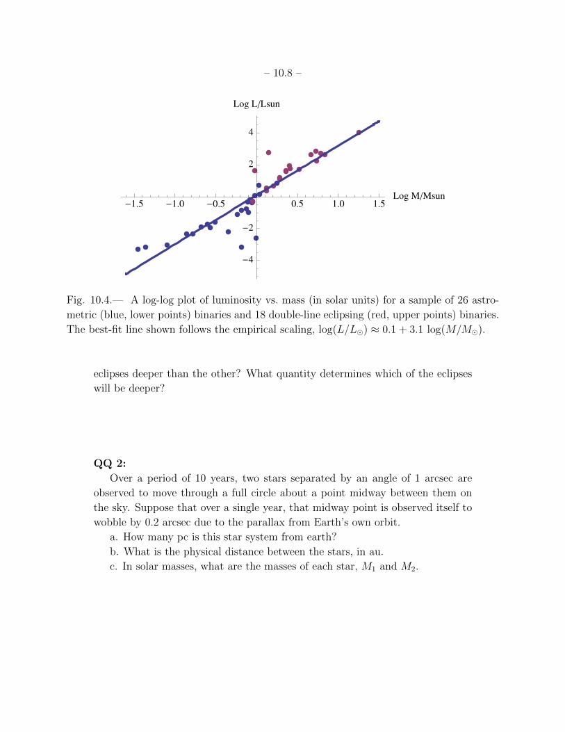
– 10.8 –
-1.5 -1.0 -0.5 0.5 1.0 1.5Log MMsun
-4
-2
2
4
Log LLsun
Fig. 10.4.— A log-log plot of luminosity vs. mass (in solar units) for a sample of 26 astro-
metric (blue, lower points) binaries and 18 double-line eclipsing (red, upper points) binaries.
The best-fit line shown follows the empirical scaling, log(L/L) ≈ 0.1 + 3.1 log(M/M).
eclipses deeper than the other? What quantity determines which of the eclipses
will be deeper?
QQ 2:
Over a period of 10 years, two stars separated by an angle of 1 arcsec are
observed to move through a full circle about a point midway between them on
the sky. Suppose that over a single year, that midway point is observed itself to
wobble by 0.2 arcsec due to the parallax from Earth’s own orbit.
a. How many pc is this star system from earth?
b. What is the physical distance between the stars, in au.
c. In solar masses, what are the masses of each star, M1 and M2.
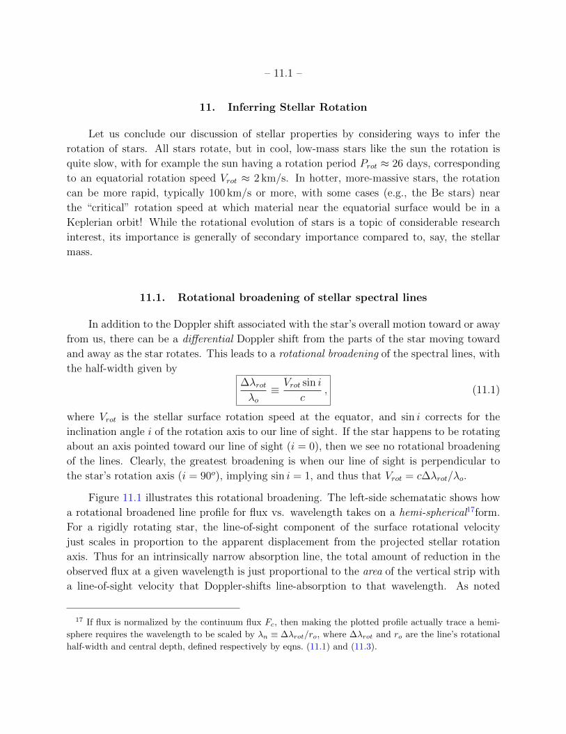
– 11.1 –
11. Inferring Stellar Rotation
Let us conclude our discussion of stellar properties by considering ways to infer the
rotation of stars. All stars rotate, but in cool, low-mass stars like the sun the rotation is
quite slow, with for example the sun having a rotation period Prot ≈ 26 days, corresponding
to an equatorial rotation speed Vrot ≈ 2 km/s. In hotter, more-massive stars, the rotation
can be more rapid, typically 100 km/s or more, with some cases (e.g., the Be stars) near
the “critical” rotation speed at which material near the equatorial surface would be in a
Keplerian orbit! While the rotational evolution of stars is a topic of considerable research
interest, its importance is generally of secondary importance compared to, say, the stellar
mass.
11.1. Rotational broadening of stellar spectral lines
In addition to the Doppler shift associated with the star’s overall motion toward or away
from us, there can be a differential Doppler shift from the parts of the star moving toward
and away as the star rotates. This leads to a rotational broadening of the spectral lines, with
the half-width given by
∆λrotλo
≡ Vrot sin i
c, (11.1)
where Vrot is the stellar surface rotation speed at the equator, and sin i corrects for the
inclination angle i of the rotation axis to our line of sight. If the star happens to be rotating
about an axis pointed toward our line of sight (i = 0), then we see no rotational broadening
of the lines. Clearly, the greatest broadening is when our line of sight is perpendicular to
the star’s rotation axis (i = 90o), implying sin i = 1, and thus that Vrot = c∆λrot/λo.
Figure 11.1 illustrates this rotational broadening. The left-side schematatic shows how
a rotational broadened line profile for flux vs. wavelength takes on a hemi-spherical17form.
For a rigidly rotating star, the line-of-sight component of the surface rotational velocity
just scales in proportion to the apparent displacement from the projected stellar rotation
axis. Thus for an intrinsically narrow absorption line, the total amount of reduction in the
observed flux at a given wavelength is just proportional to the area of the vertical strip with
a line-of-sight velocity that Doppler-shifts line-absorption to that wavelength. As noted
17 If flux is normalized by the continuum flux Fc, then making the plotted profile actually trace a hemi-
sphere requires the wavelength to be scaled by λn ≡ ∆λrot/ro, where ∆λrot and ro are the line’s rotational
half-width and central depth, defined respectively by eqns. (11.1) and (11.3).

– 11.2 –
λ
Fλ
λο (1+Vsini/c) λο (1−Vsini/c)
λο
+Vsini-Vsini
Fig. 11.1.— Left: Schematic showing how the Doppler shift from rigid body rotation of
a star (bottom) – with constant line-of-sight velocity along strips parallel to the rotation
axis – results in a hemi-spherical line-absorption-profile (top). Right: Observed rotational
broadening of lines for a sample of stars with (quite rapid) projected rotation speeds V sin i >
100 km/s.
above, the total width of the profile is just twice the star’s projected equatorial rotation
speed, V sin i.
The right panel shows a collection of observed rotationally broadened absorption lines
for a sample of quite rapidly rotating stars, i.e. with V sin i more than 100 km/s, much larger
than the ∼ 1.8 km/s rotation speed of the solar equator. The flux ratio here is relative to
the nearby “continuum” outside the line.
Note that the reduction at line-center is typically only a few percent. This is because
such rotational broadening preserves the total amount of reduced flux, meaning then that
the relative depth of the reduction is diluted when a rapid apparent rotation significantly
broadens the line.
A convenient measure for the total line absorption is the “equivalent width”,
Wλ ≡∫ ∞
0
(1− Fλ
Fc
)dλ , (11.2)
which represents the width of a “saturated rectangle” with same integrated area of reduced
flux. For a line with equivalent width Wλ and a rotationally broadened half-width ∆λrot,
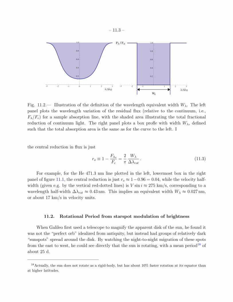
– 11.3 –
1 2 3
0.2
0.4
0.6
0.8
1.0
Wλ
Fλ/Fc
-3 -2 -1-3 -2 -1 0 1 2 3
0.2
0.4
0.6
0.8
1.0
λ/ΔλD λ/ΔλD
Fig. 11.2.— Illustration of the definition of the wavelength equivalent width Wλ. The left
panel plots the wavelength variation of the residual flux (relative to the continuum, i.e.,
Fλ/Fc) for a sample absorption line, with the shaded area illustrating the total fractional
reduction of continuum light. The right panel plots a box profle with width Wλ, defined
such that the total absorption area is the same as for the curve to the left. I
the central reduction in flux is just
ro ≡ 1− FλoFc
=2
π
Wλ
∆λrot. (11.3)
For example, for the He 471.3 nm line plotted in the left, lowermost box in the right
panel of figure 11.1, the central reduction is just ro ≈ 1−0.96 = 0.04, while the velocity half-
width (given e.g. by the vertical red-dotted lines) is V sin i ≈ 275 km/s, corresponding to a
wavelength half-width ∆λrot ≈ 0.43 nm. This implies an equivalent width Wλ ≈ 0.027 nm,
or about 17 km/s in velocity units.
11.2. Rotational Period from starspot modulation of brightness
When Galileo first used a telescope to magnify the apparent disk of the sun, he found it
was not the “perfect orb” idealized from antiquity, but instead had groups of relatively dark
“sunspots” spread around the disk. By watching the night-to-night migration of these spots
from the east to west, he could see directly that the sun is rotating, with a mean period18 of
about 25 d.
18Actually, the sun does not rotate as a rigid-body, but has about 10% faster rotation at its equator than
at higher latitudes.

– 11.4 –
Though other stars are too far away to directly resolve the stellar disk and thus make
similar direct detections of analogous “starspots”, in some cases such spots are large and
isolated enough that careful photometric measurement of the apparent stellar brightness
shows a regular modulation over the stellar rotation period P .
If the star also shows rotationally broadened spectral lines with an associated inferred
projected rotational speed Vrot sin i, then the basic relation Vrot = 2πR/P implies a constraint
on the minimum possible value for the stellar radius, Rmin = Vrot sin iP/2π.
11.3. Questions and Exercises
Quick Question 1: A line with rest wavelength λo = 500 nm is rotational
broadened to a full width of 0.5 nm. Compute the value of V sin i, in km/s.
Exercise 1: Derive eqn. (11.3) from the definitions of rotational Doppler width
∆λrot (11.1) and equivalent width Wλ (11.2), using the wavelength scaling given
in footnote 17.

– 12.1 –
12. Light Intensity and Absorption
12.1. Intensity vs. Flux
Ωrec
Aem
Irec
Iem
Iem
θ
Arec=d 2
Ωrec
Ωem=Aem cosθ/d2
dd
Irec
θ
Fig. 12.1.— Left: The intensity Iem emitted into a solid angle Ωrec located along a direction
that makes an angle θ with the normal of the emission area Aem. Right: The intensity Irecreceived into an area Arec = d2Ωrec at a distance d from the source with projected solid
angle Ωem = Aem cos θ/d2. Since the emitted and received energies are equal, we see that
Iem = Irec, showing that intensity is invariant with distance d.
Our initial introduction of surface brightness characterized it as a flux confined within
an observed solid angle, F/Ω. But actually the surface brightness is directly related to a
more general and fundamental quantity known as the Specific19 Intensity I. In the exterior
of stars, the intensity is set by the surface brightness I = F/Ω, but it can also be specified
in the stellar interior, where it characterizes the properties of the radiation field as energy
generated in the core is transported to the surface.
A simple analog on earth would be an airplane flying through a cloud. Viewed from
19 Often this “Specific” qualifer is dropped, leaving just “Intensity”.
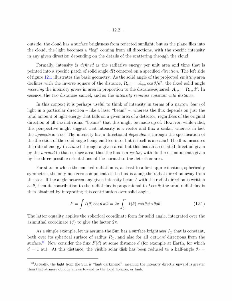
– 12.2 –
outside, the cloud has a surface brightness from reflected sunlight, but as the plane flies into
the cloud, the light becomes a “fog” coming from all directions, with the specific intensity
in any given direction depending on the details of the scattering through the cloud.
Formally, intensity is defined as the radiative energy per unit area and time that is
pointed into a specific patch of solid angle dΩ centered on a specified direction. The left side
of figure 12.1 illustrates the basic geometry. As the solid angle of the projected emitting area
declines with the inverse square of the distance, Ωem = Aem cos θ/d2, the fixed solid angle
receiving the intensity grows in area in proportion to the distance-squared, Arec = Ωrecd2. In
essence, the two distances cancel, and so the intensity remains constant with distance.
In this context it is perhaps useful to think of intensity in terms of a narrow beam of
light in a particular direction – like a laser “beam” –, whereas the flux depends on just the
total amount of light energy that falls on a given area of a detector, regardless of the original
direction of all the individual “beams” that this might be made up of. However, while valid,
this perspective might suggest that intensity is a vector and flux a scalar, whereas in fact
the opposite is true. The intensity has a directional dependence through the specification of
the direction of the solid angle being emitted into, but it itself is a scalar! The flux measures
the rate of energy (a scalar) through a given area, but this has an associated direction given
by the normal to that surface area; thus the flux is a vector, with its three components given
by the three possible orientations of the normal to the detection area.
For stars in which the emitted radiation is, at least to a first approximation, spherically
symmetric, the only non-zero component of the flux is along the radial direction away from
the star. If the angle between any given intensity beam I with the radial direction is written
as θ, then its contribution to the radial flux is proportional to I cos θ; the total radial flux is
then obtained by integrating this contribution over solid angle,
F =
∫I(θ) cos θ dΩ = 2π
∫ π
0
I(θ) cos θ sin θdθ . (12.1)
The latter equality applies the spherical coordinate form for solid angle, integrated over the
azimuthal coordinate (φ) to give the factor 2π.
As a simple example, let us assume the Sun has a surface brightness I that is constant,
both over its spherical surface of radius R, and also for all outward directions from the
surface.20 Now consider the flux F (d) at some distance d (for example at Earth, for which
d = 1 au). At this distance, the visible solar disk has been reduced to a half-angle θd =
20Actually, the light from the Sun is “limb darkenend”, meaning the intensity directly upward is greater
than that at more oblique angles toward to the local horizon, or limb.
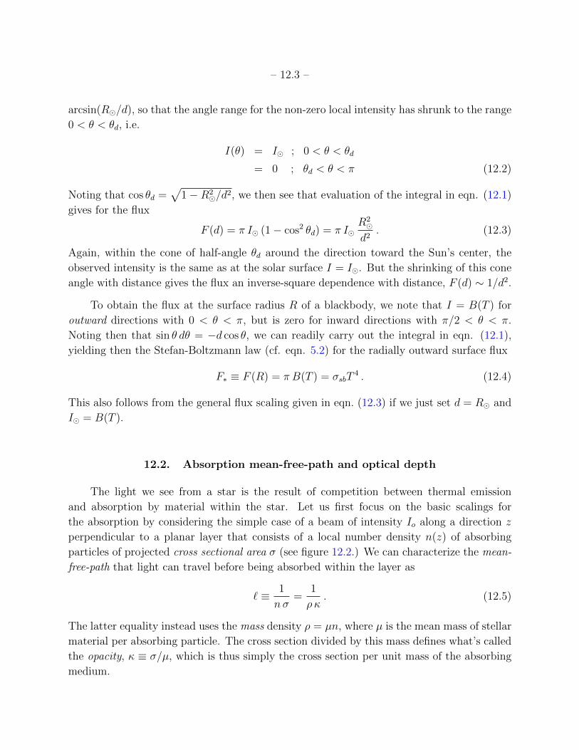
– 12.3 –
arcsin(R/d), so that the angle range for the non-zero local intensity has shrunk to the range
0 < θ < θd, i.e.
I(θ) = I ; 0 < θ < θd
= 0 ; θd < θ < π (12.2)
Noting that cos θd =√
1−R2/d
2, we then see that evaluation of the integral in eqn. (12.1)
gives for the flux
F (d) = π I (1− cos2 θd) = π IR2
d2. (12.3)
Again, within the cone of half-angle θd around the direction toward the Sun’s center, the
observed intensity is the same as at the solar surface I = I. But the shrinking of this cone
angle with distance gives the flux an inverse-square dependence with distance, F (d) ∼ 1/d2.
To obtain the flux at the surface radius R of a blackbody, we note that I = B(T ) for
outward directions with 0 < θ < π, but is zero for inward directions with π/2 < θ < π.
Noting then that sin θ dθ = −d cos θ, we can readily carry out the integral in eqn. (12.1),
yielding then the Stefan-Boltzmann law (cf. eqn. 5.2) for the radially outward surface flux
F∗ ≡ F (R) = π B(T ) = σsbT4 . (12.4)
This also follows from the general flux scaling given in eqn. (12.3) if we just set d = R and
I = B(T ).
12.2. Absorption mean-free-path and optical depth
The light we see from a star is the result of competition between thermal emission
and absorption by material within the star. Let us first focus on the basic scalings for
the absorption by considering the simple case of a beam of intensity Io along a direction z
perpendicular to a planar layer that consists of a local number density n(z) of absorbing
particles of projected cross sectional area σ (see figure 12.2.) We can characterize the mean-
free-path that light can travel before being absorbed within the layer as
` ≡ 1
nσ=
1
ρ κ. (12.5)
The latter equality instead uses the mass density ρ = µn, where µ is the mean mass of stellar
material per absorbing particle. The cross section divided by this mass defines what’s called
the opacity, κ ≡ σ/µ, which is thus simply the cross section per unit mass of the absorbing
medium.
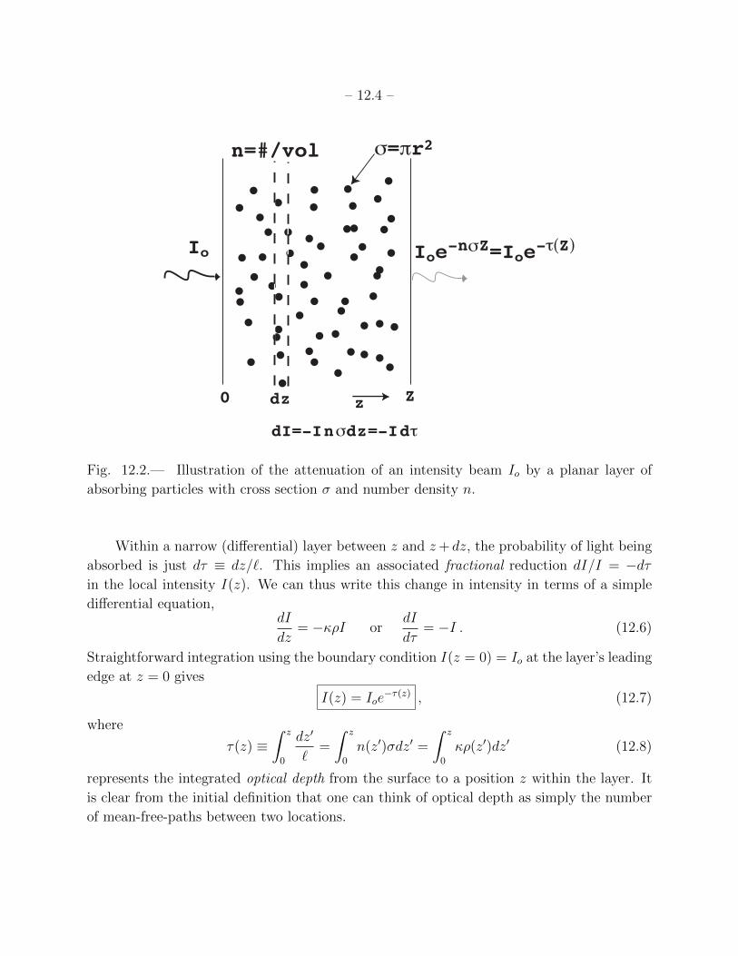
– 12.4 –
Io
0 z Z
σ=πr2n=#/vol
Ioe-nσZ=Ioe-τ(Z)
dI=-Inσdz=-Idτ
dz
Fig. 12.2.— Illustration of the attenuation of an intensity beam Io by a planar layer of
absorbing particles with cross section σ and number density n.
Within a narrow (differential) layer between z and z+ dz, the probability of light being
absorbed is just dτ ≡ dz/`. This implies an associated fractional reduction dI/I = −dτin the local intensity I(z). We can thus write this change in intensity in terms of a simple
differential equation,dI
dz= −κρI or
dI
dτ= −I . (12.6)
Straightforward integration using the boundary condition I(z = 0) = Io at the layer’s leading
edge at z = 0 gives
I(z) = Ioe−τ(z) , (12.7)
where
τ(z) ≡∫ z
0
dz′
`=
∫ z
0
n(z′)σdz′ =
∫ z
0
κρ(z′)dz′ (12.8)
represents the integrated optical depth from the surface to a position z within the layer. It
is clear from the initial definition that one can think of optical depth as simply the number
of mean-free-paths between two locations.
– 12.5 –
12.3. Inter-stellar extinction and reddening
One practical example of such exponential reduction of light by absorption is the case
of inter-stellar “extinction” of starlight. The space between stars – called the Inter-Stellar
Medium (ISM) – is not completely empty, but contains a certain amount of gas and dust.
Compared to a stellar atmosphere, or indeed even to a strong terrestrial vacuum, the density
is very small, often only a few atoms per cubic centimeter, or a few hundred dust particles per
cubic kilometer. But over the huge distances between stars, the associated optical depth τ
for extinction of the star’s light by scattering and/or absorption can become quite significant,
leading to a substantial reduction in the star’s apparent brightness.
For a star of radius R and surface intensity Io, the luminosity is L = 4π2R2Io, and in
the absence of any absorption the observed flux at a distance d is just Fo(d) = L/4πd2 =
πIo(R/d)2. But in the case with ISM absorption, this is again (cf. eqn. 12.7) reduced by the
optical depth exponential absorption factor
Fabs(d) = Fo(d)e−τ . (12.9)
The level of this ISM absorption can also be characterized in terms of the number of mag-
nitudes of extinction,
A ≡ mobs −mo = 2.5 log
(FoFabs
)= 2.5 τ log e ≈ 1.08 τ . (12.10)
In interpreting the observed magnitude of a “standard candle” star with known lumi-
nosity, the failure to account for any such extinction can lead to an inferred distance dinfthat overestimates of the star’s true distance d.
In practice, interstellar extinction is generally dominated by the opacity associated with
interstellar grains of dust. For large dust grains, the absorption cross section just depends
on the physical size, for example given by σ = πr2 for spherical grains of radius r.
But interstellar dust grains are often very tiny, even microscopic, with sizes of less than
a micron, and so comparable to the wavelength of optical light. For light in the red or
infra-red that has a wavelength larger than the dust size, λ > r, the effective cross section,
and thus the associated dust opacity, is reduced, because, in loose sense, the dust particle
can only interact with a fraction of the light wave. Because this redder, longer wavelength
light is less strongly absorbed than the bluer, shorter wavelengths, the remaining light tends
to appear “reddened”, much in the same way as the sun’s light at sunset.
This reddening can be quantified in terms of a formal color excess, defined in terms of
– 12.6 –
the standard B and V filters of the Johnson photometric system,
EB−V ≡ (B − V )obs − (B − V )int , (12.11)
where the subscripts stand for “observed” and “intrinsic”. This color excess tends to increase
with increasing visual extinction magnitude AV . If the intrinsic colors are known (e.g., from
the star’s spectral type), then, for a given model of the wavelength dependence of the opacity,
measuring this color excess makes it possible to estimate of the visual extinction magnitude
AV ≡ Vobs − Vint. Among other things, this allows one to reduce or remove the error in
determining the stellar distance.
The detailed variation of dust opacity depends on the size, shape, and composition of
the dust, but often it is approximated as scaling as an inverse power law in wavelength, i.e.
κ(λ) ∼ λ−β,
where the power index (a.k.a. “reddening exponent”) ranges from β ≈ 1 for “Mie scattering”
to β ≈ 4 for “Rayleigh scattering”.
The latter is a good approximation for scattering by air molecules and dust in the earth’s
atmosphere. The scattering of blue light out of the direction from the sun makes the sunset
red, while all that scattered blue light makes the sky blue.
For ISM dust, the weaker β ≈ 1 scaling is more appropriate, but even this can make a
marked difference in the level of extinction for different wavelengths.
For example, if a star has an extinction AV in the visual waveband centered on λV ≈500 nm, then in the mid-infrared “M-waveband” at roughly a factor ten higher wavelength
λM ≈ 5000 nm = 5µm, the opacity, and thus the optical depth and extinction magnitude, are
all reduced by this same factor 10, AM ≈ AV /10. For a case with, say AV = 10.8 magnitudes
of visual extinction, the visual flux would be reduced by a factor e−τV = e−AV /1.08 = e−10 =
4.5× 10⁻⁵. By contrast, in this mid-IR M-band, the factor ten lower extinction magnitude
AM = 1.08 implies a much weaker reduction, now just a factor e−τM = e−AM/1.08 = e−1 =
0.36.
Stars are typically formed out of interstellar gas and dust in very dense molecular
clouds, which often have 10 or 20 magnitudes of visual extinction (AV ≈ 10−20), essentially
completely obscuring them at visual wavelengths. But such stars can nonetheless be readily
observed with minimal extinction in mid-IR (few microns) or far-IR (millimeter) wavebands.
This fact has spurred efforts to build large infra-red telescopes, both on the ground and
in space. The ground-based telescopes are placed at high altitudes of very dry deserts, to
minimize the effect of IR absorption by water vapor in the earth’s atmosphere. Another
issue is to keep the IR detectors very cold, to reduce the thermal emission background.
– 12.7 –
12.4. Questions and Exercises
Quick Question 1
(a.) Suppose spherical dust grains have a radius r = 0.1 cm and individual mass
density ρg = 1 g/cm3. What is their cross section σ, mass m, and associated
opacity κ?
(b.) If the number density of these grains is nd = 1 cm−3, what is the mass
density of dust ρd and the mean free path ` for light?
(c.) What is the optical depth at a physical depth 1 m into a planar layer of such
dust absorbers?
(d.) What fraction of impingent intensity Io makes it to this depth?
Quick Question 2: Derive expressions for dinf/d in terms of both the absorption
magnitude A and the optical depth τ .
– A.1 –
A. Atomic Energy Levels and Transitions
As a basis for the examination in part II of how these various inferred basic properties of
stars can be understood in terms of the physics of stellar structure, let us next consider some
key physical underpinnings for interpreting observed stellar spectra. Specifically, this section
discusses the simple Bohr model of the Hydrogen atom, while the next section reviews the
Boltzmann description for excitation and ionization of atoms.
A.1. The Bohr atom
The discretization of atomic energy that leads to spectral lines can be understood semi-
quantitatively through the simple Bohr model of the Hydrogen atom. In analogy with planets
orbiting the sun, this assumes that electrons of charge −e and mass me are in a stable circular
orbit around the atomic nucleus (for hydrogen just a single proton) of charge +e whose mass
mp is effectively infinite (mp/me = 1836 1) compared to the electron. The electrostatic
attraction between these charges21 then balances the centrifugal force from the electron’s
orbital speed v along a circular orbit of radius r,
e2
r2=mev
2
r. (A1)
In classical physics, this orbit could, much like a planet going around the sun, have any
arbitrary radius. But in the microscopic world of atoms and electrons, such classical physics
has to be modified – indeed replaced – by quantum mechanics22. Just as a light wave has its
energy quantized into discrete bundles called photons, it turns out that the orbital energy
of an electron is also quantized into discrete levels, much like the steps of a staircase. The
basic reason stems from the fact that, in the ghostly world of quantum mechanics, electrons
are themselves not entirely discrete particles, but rather, much like light, can also have a
“wavelike” character. In fact any particle with momentum p = mv has an associated “de
21The force on the left-side of (A1) is written here for CGS units, for which r is in cm and the electron
charge magnitude is 4.8× 10⁻¹⁰ statcoulomb (a.k.a. “esu”), where statcoulomb2= erg cm = dyne cm2. For
MKS units, for which the charge is 1.6×10⁻¹⁹ Coulomb, there is an additional proportionality factor 1/4πεo,
where εo = 8.85× 10⁻¹² Coulomb2/J/m is the “permittivity of free space”. For simplicity, we use the CGS
form here.
22In the classic sci-fi flick Forbidden Planet, the chief engineer of a spaceship quips, “I’ll bet any quantum
mechanic in the space force would give his right arm to fool around with this gadget”.
– A.2 –
Broglie wavelength” given by
λ =h
mv, (A2)
where again, h is Planck’s constant.
This wavy fuzziness means an orbiting electron cannot be placed at any precise location,
but is somewhat spread along the orbit. But then to avoid “interfering with itself”, integer
multiples n of this wavelength should match the orbital circumference 2πr, implying
nλ = 2πr =nh
mv. (A3)
Note that Planck’s constant itself has units of momentum times distance23, which represents
an angular momentum. So another way to view this is that the electron’s orbital angular
momentum J = mvr must likewise be quantized,
J = mvr = n~ , (A4)
where ~ ≡ h/2π is a standard notation shortcut. The integer index n is known as the
principal quantum number.
The quantization condition in eqn. (A3) or (A4) implies that the orbital radius can only
take certain discrete values rn, numbered by the level n,
rn = n2 ~2
mee2= n2 r1 , (A5)
which for the ground state, n = 1, reduces to the “Bohr radius”, r1 ≈ 0.529A = 0.0529 nm.
More generally, this implies that most atoms have sizes of a few Angstrom (1 A ≡ 0.1 nm).
It is also useful to cast this quantization in terms of the associated orbital energy. The
total orbital energy is a combination of the negative potential energy U = −e2/r, and the
positive kinetic energy T = mev2/2. Using the orbital force balance eqn. (A1), we find that
the total energy is
En = − e2
2rn= −mee
4
2~2
1
n2= −E1
n2= En , (A6)
where
E1 ≡mee
4
2~2=
e2
2r1
= 2.2× 10⁻¹¹erg = 13.6 eV = E1 (A7)
23Or also, energy× time, which when used with Heisenberg’s Uncertainty Principle ∆E∆t ∼> h, will lead
us to conclude that an atomic state with finite lifetime tlife must have a finite width or “fuzziness” in its
energy ∆E ∼ h/tlife. This leads to what is known as “natural broadening” of spectral lines.
– A.3 –
denotes the ionization (a.k.a. binding) energy of Hydrogen from the ground state (with
n = 1). Figure A.1 gives a schematic rendition of the energy levels of Hydrogen, measured
in electron Volts (eV), which is the energy gained when a charge of one electron falls through
an electrical potential of one volt.
A.2. Emission vs. Absorption line spectra
When an electron changes from one level with quantum number m to another with
quantum number n, then the associated change in energy is
∆Emn = E1
(1
n2− 1
m2
)= 13.6 eV
(1
n2− 1
m2
). (A8)
If m > n in eqn. (A8), this represents a positive energy, ∆Emn > 0, which can be emitted
as a photon of just that energy hν = ∆Emn. Conversely, if m < n, we have ∆Emn < 0,
implying that energy must be supplied externally, for example by absorption of a photon of
just the right energy, hν = −∆Emn. These processes are called “bound-bound” emission
and absorption, because they involve transitions between two bound levels of electrons in an
atom.
Bound-bound absorption is the basic process responsible for the absorption line spec-
trum seen from the surface of most stars. As illustrated in the right panel of figure 6.2, the
relatively cool atoms near the surface of the star absorb the light from the underlying layers.
On the other hand, for gas in interstellar space, the atoms are generally viewed against
a dark background, instead of the bright back-lighting of a star. If the gas is dense and hot
enough that collisions among the atoms occur with enough frequency and enough energy
to excite the bound electrons in the atoms to some level above the ground state, then the
subsequent spontaneous decay to some lower level will emit photons, and so result in an
emission-line spectrum.
Recall again that figure 6.2 illustrates the basic processes for production of emission and
absorption line spectra in both the laboratory and astrophysics.
A.3. Line wavelengths for term series
Instead of photon energy, light is more commonly characterized by its wavelength λ =
c/ν = hc/E. Using this conversion in eqn. (A8), we find the wavelength of a photon emitted
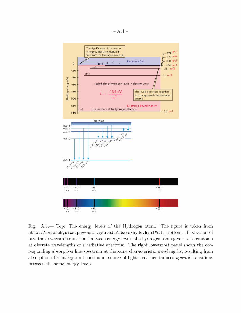
– A.4 –
Fig. A.1.— Top: The energy levels of the Hydrogen atom. The figure is taken from
http://hyperphysics.phy-astr.gsu.edu/hbase/hyde.html#c3 . Bottom: Illustration of
how the downward transitions between energy levels of a hydrogen atom give rise to emission
at discrete wavelengths of a radiative spectrum. The right lowermost panel shows the cor-
responding absorption line spectrum at the same characteristic wavelengths, resulting from
absorption of a background continuum source of light that then induces upward transitions
between the same energy levels.
– A.5 –
by transition from a level m to a lower level n is
λmn =λ1
1n2 − 1
m2
=912A
1n2 − 1
m2
, (A9)
where
λ1 ≡hc
E1
=h3c
2π2mee4= 91.2 nm = 912 A (A10)
is the wavelength at what is known as the Lyman limit, corresponding to a transition to the
ground state n = 1 from an arbitrarily high bound level with m→∞. Of course, transitions
from a lower level m to a higher level n require absorption of a photon, with the wavelength
now given by the absolute value of eqn. (A9).
The lower level of a transition defines a series of line wavelengths for transitions from all
higher levels. For example, the Lyman series represents all transitions to/from the ground
state n = 1. Within each series, the transitions are denoted in sequence by a lower case greek
letter, e.g. λ21 = (4/3) 912 = 1216 A is called Lyman-α, while λ31 = (9/8)912 = 1026 A is
called Lyman-β, etc. The Lyman series all falls in the ultraviolet (UV) part of the spectrum,
which due to UV absorption by the earth’s atmosphere is generally not possible to observe
from ground-based observatories.
More accessible is the Balmer series, for transitions between n = 2 and higher levels
with m = 3, 4, etc., which are conventionally denoted Hα, Hβ, etc. These transitions are
pretty well positioned in the middle of the visible, ranging from λ32 = 6566 A for Hα to
λ∞2 = 3648 A for the Balmer limit.
The Paschen series, with lower level n = 3, is generally in the InfraRed (IR) part of the
spectrum. Still higher series are at even longer wavelengths.
A.4. Questions and Exercises
Quick Questions 1:
(a) Compute the wavelengths (in nm) for Paschen-α λ43 and the Paschen limit
λ∞3.
(b) What are the associated changes in energy (in eV), ∆E43 and ∆E∞3.
Exercise 1: For an electron and proton that are initially a distance r apart,
show that the energy needed to separate them to an arbitrarily large distance is
– A.6 –
given by U(r) ≡ −e2/r. Use the resulting potential energy U(r) together with
the orbital kinetic energy T = mev2/2 to derive the expressions in eqn. (A6) for
the total energy E = U + T .
Exercise 2: Confirm the validity of eqn. (A6) by using eqn. (A1) to show
that E = U/2 = −T , where U , T , E are the potential, kinetic, and total energy
of an orbiting electron. (Note: this result is sometimes referred to as a corollary
of the Virial Theorum for bound systems, which is discussed elsewhere in these
notes.)
– B.1 –
B. Equilibrium Excitation and Ionization Balance
B.1. Boltzmann equation
A key issue for forming a star’s absorption spectrum is the balance of processes that
excite and de-excite the various energy levels of the atoms. In addition to the photon
absorption and emission processes discussed above, atoms can also be excited or de-excited
by collisions with other atoms. Since the rate and energy of collisions depends on the gas
temperature, the shuffling among the different energy levels also depends sensitively on the
temperature.
Under a condition called thermodynamic equilibrium, the population of electrons gets all
mixed up; then if these levels were all equal in energy, the numbers in each level i would just
be proportional to the number of quantum mechanical states, gi, associated with the orbital
and spin state of the electrons in that level24. But between a lower level i and upper level
j with an energy difference ∆Eij, the relative population is also weighted by an exponential
term called the Boltzmann factor,
njni
=gjgie−∆Eij/kT , (B1)
where k = 1.38× 10⁻¹⁶erg/K is known as Boltzmann’s constant. At low temperature, with
the thermal energy much less than the energy difference, kT ∆Eij, there are relatively
very few atoms in the more excited level j, nj/ni → 0. Conversely, at very high temperature,
with the thermal energy much greater than the energy difference, kT ∆Eij, the ratio just
becomes set by the statistical weights, nj/ni → gj/gi.
As the population in excited levels increases with increased temperature, there are thus
more and more atoms able to emit photons, once these excited states spontaneously decay
to some lower level. This leads to an increased emission of the associated line transitions.
On the other hand, at lower temperature, the population balance shifts to lower levels.
So when these cool atoms are illuminated by continuum light from hot layers, there is a net
absorption of photons at the relevant line wavelengths, leading to a line-absorption spectrum.
24These orbital and spin states are denoted by quantum mechanical numbers ` and m, which thus supple-
ment the principal quantum number n.

– B.2 –
B.2. Saha equation for ionization equilibrium
At high temperatures, the energy of collisions can become sufficient to overcome the full
binding energy of the atom, allowing the electron to become free, and thus making the atom
an ion, with a net positive charge. For atoms with more than a single proton, this process of
ionization can continue through multiple stages up to the number of protons, at which point
it is completely stripped of electrons. Between an ionization stage i and the next ionization
stage i+ 1, the exchange for any element X can be written as
Xi+1 ↔ Xi + e− . (B2)
In thermodynamic equilibrium, there develops a statistical balance between the neigh-
boring ionization stages that is quite analogous to the Boltzmann equilibrium for bound
levels given in eqn. (B1). But now the ionized states consist of both ions, with many discrete
energy levels, and free electrons. The number of bound states of an ion in ionization stage i
is now given by something called the partition function, which we will again write as gi. But
to write the equilibrium balance, we now need also to find an expression for the number of
states available to the free electron.
For this we return again to the concept of the de Broglie wavelength, writing this now for
an electron with thermal energy kT . Using the relation p2/2me = πkT between momentum
and thermal energy, the thermal de Broglie wavelength is
Λ =h
p=
h√2πmekT
. (B3)
For each of the two electron spins, the total number of free-electron states available per unit
volume is 2/Λ3. For electron number density ne, this then implies there are 2/neΛ3 states
for each free electron.
Using this, we can then describe the ionization balance between neighboring stages i
and i+ 1 through the Saha-Boltzmann equation,
n(Xi+1)
n(Xi)=gi+1
gi
(2
neΛ3
)e−∆Ei/kT , (B4)
where ∆Ei is the ionization energy from stage i, and ne is the free electron number density.
The gi now represent what’s known as the “partition function”, which characterizes the total
number of bound states available for each ionization stage i; the large (and formally even
divergent!) number of bound states can make it difficult to compute the partition functions
gi, but for Hydrogen under conditions in stellar envelopes, one obtains a typical partition
ratio g1/g0 ≈ 10−3.
– B.3 –
Throughout a normal star, the electron state factor in parentheses is typically a huge
number25. For example, for conditions in a stellar atmosphere, it is typically of order 1010.
This large number of states acts like a kind of “attractor” for the ionized state. It means
the numbers in the more vs. less ionized states can be comparble even when the exponential
Boltzman factor is very small, with a thermal energy that is well below the ionization energy,
i.e. kT ≈ ∆Ei/10.
For example, hydrogen in a stellar atmosphere typically starts to become ionized at a
temperature of about T ≈ 104K, even though the thermal energy is only kT ≈ 0.86 eV,
and thus much less than the hydrogen ionization energy Ei = 13.6 eV, implying a Boltzman
factor e−13.6/0.86 = 1.4 × 10⁻⁷. For a partition ratio g1/g0 ≈ 10−3, we thus obtain roughly
equal fractions of Hydrogen in neutral and ionized states at modest temperature of just
T ≈ 104K.
B.3. Questions and Exercises
Quick Question 1: The n = 2 level of Hydrogen has g2 = 8 states, while the
ground level has just g1 = 2 states. Using the energy difference ∆E21 from the
Bohr atom, compute the Boltzmann equilibrium number ratio n2/n1 of electrons
in these levels for a temperature T = 100, 000 K.
Exercise 1: For a medium of pure hydrogen with total number density nH =
1010 cm−3, compute the temperature T for unit number ratio of n0/n1 = 1 for
neutral/ionized Hydrogen, assuming a ratio g0/g1 = 2 for the neutral/ionized
states.
25As discussed later, it only becomes order unity in very compressed conditions, like in the interior of a
white dwarf star, which is thus said to be electron degenerate; see sections 16 and 17 of part II.
Related Documents