Phylogenetically aligned component analysis

Methods Ecol Evol. 2021;12:359–372. wileyonlinelibrary.com/journal/mee3  |  359© 2020 British Ecological Society

1  | INTRODUC TION

Biological phenotypes are highly multivariate; containing sets of traits—or trait dimensions—that covary with one another to a greater or lesser degree (Adams & Collyer, 2019a; Goswami & Polly, 2010; Klingenberg, 2008; Olson & Miller, 1958). Increasingly, evolutionary biologists are characterizing phenotypes multivari-ately; evaluating trends in more than one trait simultaneously (e.g. Caetano & Harmon, 2019; Friedman et al., 2016; Price et al., 2010),

or describing evolutionary changes in complex multidimensional phenotypes (e.g. Felice & Goswami, 2018; Martinez et al., 2018; Sherratt et al., 2016; Zelditch et al., 2017). This, in turn, has lead to the development of multivariate phylogenetic comparative meth-ods, which facilitate the evaluation of macroevolutionary trends in multivariate phenotypes across the tree of life and in light of phy-logenetic non-independence (e.g. Adams, 2014a, 2014b; Adams & Collyer, 2018b; Bartoszek et al., 2012; Bastide et al., 2018; Revell & Harmon, 2008).

Received: 12 April 2020  |  Accepted: 25 September 2020

DOI: 10.1111/2041-210X.13515

R E S E A R C H A R T I C L E

Phylogenetically aligned component analysis

Michael L. Collyer1  | Dean C. Adams2

1Department of Science, Chatham University, Pittsburgh, PA, USA2Department of Ecology, Evolution, and Organismal Biology, Iowa State University, Ames, IA, USA

CorrespondenceMichael L. CollyerEmail: [email protected]

Funding informationNational Science Foundation, Grant/Award Number: DBI-1902694 and DBI-1902511

Handling Editor: Simone Blomberg

Abstract1. It has become common in evolutionary biology to characterize phenotypes multi-

variately. However, visualizing macroevolutionary trends in multivariate datasets requires appropriate ordination methods.

2. In this paper we describe phylogenetically aligned component analysis (PACA): a new ordination approach that aligns phenotypic data with phylogenetic signal. Unlike phylogenetic principal component analysis (Phy-PCA), which finds an align-ment of a principal eigenvector that is independent of phylogenetic signal, PACA maximizes variation in directions that describe phylogenetic signal, while simulta-neously preserving the Euclidean distances among observations in the data space.

3. We demonstrate with simulated and empirical examples that with PACA, it is possible to visualize the trend in phylogenetic signal in multivariate data spaces, irrespective of other signals in the data. In conjunction with Phy-PCA, one can visualize both phylogenetic signal and trends in data independent of phylogenetic signal.

4. Phylogenetically aligned component analysis can distinguish between weak phy-logenetic signals and strong signals concentrated in only a portion of all data di-mensions. We provide empirical examples that emphasize the difference. Use of PACA in studies focused on phylogenetic signal should enable much more precise description of the phylogenetic signal, as a result.

5. Overall, PACA will return a projection that shows the most phylogenetic signal in the first few components, irrespective of other signals in the data. By comparing Phy-PCA and PACA results, one may glean the relative importance of phyloge-netic and other (ecological) signals in the data.

K E Y W O R D S

multivariate, ordination, phylogenetic, principal component, singular value decomposition

360  |    Methods in Ecology and Evolu on COLLYER and adaMS

Visualization of patterns in multivariate data spaces is an import-ant component of phylogenetic comparative methods, especially when comparing multidimensional phenotypes (Adams & Collyer, 2018a, 2019b). Presently, there are two approaches commonly used to vi-sualize multivariate trends for continuous variables: the ‘phylomor-phospace’ approach (Rohlf, 2002; Sidlauskas, 2008) and phylogenetic principal component analysis (Phy-PCA; Revell, 2009; see also Polly et al., 2013). With both approaches, PCA is performed and the esti-mated ancestral characters for phylogenetic nodes can be projected into the space described by principal component (PC) vectors, along with the vectors of values for species (taxa) from the phylogeny, as a means of visualizing multivariate trends. The chief difference between phylomorphospace analysis (PA) and Phy-PCA is that the former finds the ordinary least squares (OLS) mean (centre of gravity) of the data space and performs a rigid-rotation of the data space to align with PCs and the latter finds the generalized least squares (GLS) mean of the data space, which culminates in an oblique projection of residuals that are independently distributed with respect to phylogeny (Polly

et al., 2013). Only when data are species' traits (rather than observa-tions at the individual level) are these methods applicable, but PCA can be performed likewise on individual-level multivariate data (e.g. Vaux et al., 2018). (Table 1 provides a brief overview of these and other sim-ilar methods.) Because phylogenetic PCs are 'evolutionarily indepen-dent' Revell (2009), one might consider using both PA and Phy-PCA to discern among possible explanations for major dispersion trends in multivariate traits. An obvious difference in the dispersion of values in PC plots from PA and Phy-PCA might suggest factors other than phy-logeny account for trait variation. An obvious difference in the disper-sion of values in PC plots from PA and Phy-PCA might suggest factors other than phylogeny account for trends in the multivariate data space.

Assessment of phylogenetic signal in multivariate data is also an important component of phylogenetic comparative methods, espe-cially for understanding the tendency for closely related taxa to dis-play similar trait values (Blomberg et al., 2003). Phylogenetic signal can be measured in various ways, but one statistic that is commonly used is Blomberg et al.'s (2003) K statistic. This statistic finds the ratio of

Terms Brief description

Multivariate data Data comprising more than one, and often many variables. Some traits, like ‘shape’ described by variables from geometric morphometric methods (Rohlf & Slice, 1990) are necessarily multivariate, as the variables have no independent meaning

Species data Multivariate data with observations at the species level, rather than the individual level. This distinction is important because species are represented by a signal observation even if species comprise individuals with substantial variation. Only with species data can analyses using phylogenetic covariance matrices be considered

Phylogenetic covariance matrix

An n × n matrix of phylogenetic covariances based on patristic distances from a phylogenetic tree

Principal component analysis (PCA)

A standard analysis that decomposes a covariance or correlation matrix into matrices of eigenvectors and eigenvalues. Projection of data onto eigenvectors (principal components) allows visualization of multivariate trends in fewer dimensions

Phylomorphospace analysis (PA)

PCA performed on a covariance or correlation matrix estimated from species data (typically morphology, but could be behaviour, physiology or life-history traits), coupled with projection of estimated ancestral states for phylogenetic nodes onto a principal component (PC) plot (Rohlf, 2002; Sidlauskas, 2008). The covariance or correlation matrix is estimated with ordinary least squares (OLS)

Phylogenetic PCA PCA performed on a covariance or correlation matrix estimated from species data, accounting for the phylogenetic non-independence of species traits. This is accomplished with generalized least squares (GLS) estimation of a covariance or correlation matrix, utilizing a phylogenetic covariance matrix (Revell, 2009). Compared to PA, Phy-PCA finds a principal component (major axis) that is mostly independent of phylogeny

Two-block partial least squares analysis (PLS)

Singular value decomposition (SVD) of the cross-products between two matrices, used to assess matrix covariation (Rohlf & Corti, 2000). A PLS scatterplot projects data onto principal ‘left’ and ‘right’ singular vectors to visualize covariation

Phylogenetically aligned component analysis (PACA)

Like PLS, a SVD of the cross-products between two matrices, but one matrix is a phylogenetic covariance matrix and the intent is to visualize trends in a set of multivariate data with alignment to phylogenetic signal

TA B L E 1   Summary of terms for data and methods used or described in this paper

     |  361Methods in Ecology and Evolu onCOLLYER and adaMS

variances calculated with and without correction by phylogenetic GLS (assuming a Brownian motion model of evolutionary divergence), and has been generalized for multivariate data by Adams (2014a). The mul-tivariate measurement of K, Kmult, will be the same whether measured on the original continuous data or their PC scores from PA or Phy-PCA (a property we illustrate in this paper) as the Euclidean distances among observations are retained after projection (Polly et al., 2013).

The reason PA and Phy-PCA are useful data-visualization tools for phylogenetic signal is that both involve projection of estimated ancestral trait values and phylogenetic tree edges, illustrating pat-terns of diversification in phylogenies. One would expect with a PC projection in PA that if phylogenetic signal is strong, estimated an-cestral trait values will align strongly with the first PC, that is, the variance among estimated ancestral trait values will be largest on this axis. Multiple signals (e.g. signal due to ecological variation, in addition to phylogenetic signal) can influence the orientation of PCs and thus contribute to the relative amount of phylogenetic signal in each PC from PA. For example, morphological variation associ-ated with planktivory in fish species might contribute to orienta-tion of the first PC in PA, as well as evolutionary diversification (see Friedman et al., 2016), as the OLS estimation of a covariance matrix neither explicitly controls for the non-independence of observa-tions due to phylogeny nor explicitly aligns with phylogeny. It should be noted that Rohlf (2002) suggested that one could perform PA by including estimated ancestral trait values as data in the calculation of a covariance matrix. This procedure would indeed align (or bias) the first PC more so towards phylogenetic signal, but at the risk of obscuring other trends in the data space, and producing PC scores that have variances that do not sum to the total variance in the data.

By contrast, one might assume if Phy-PCA rotates a data space to phylogenetically independent axes, PC scores are also independent of phylogenetic signal. This is not true, although phylogenetic signal might be minimized along the first Phy-PC. Rather, Phy-PCA projects GLS-centred residuals that are not transformed by phylogenetic co-variances, meaning that the amount of dispersion in PC projections is the same as the amount of dispersion about the GLS mean in the orig-inal data space (Polly et al., 2013). Therefore, Phy-PCA finds a rotation of the data space about the GLS mean that is rather independent of phylogenetic signal in the first Phy-PC, but phylogenetic signal is re-tained throughout all Phy-PCs, that is, Phy-PCA redistributes the phy-logenetic signal to lower PCs. Therefore, PA will reveal predominant trends in the multivariate species data in the first few PCs; Phy-PCA will reveal trends, independent of phylogeny, but neither explicitly reveals trends most associated with phylogenetic signal. Such a ca-pability would greatly complement Phy-PCA and allow researchers to consider the alternative signals in their multivariate data spaces.

Here we present a conceptual framework to explicitly reveal trends in multivariate data spaces most associated with phylogenetic signal, which is a valuable complement to Phy-PCA. This framework is similar to other methods that involve aligning matrices through singular value decomposition (SVD) of matrix cross-products. For example, in geomet-ric morphometrics, Procrustes superimposition (Rohlf & Slice, 1990) in-volves finding the cross-product between two sets of landmarks and

developing a rotation matrix via SVD of this cross-product in order to rotate the second matrix to align with the first. Likewise, the meth-ods of partial least squares (PLS) correlation and regression (Abdi & Williams, 2013) involve finding the cross-product between two sets of mean-centred or standardized data and using SVD to obtain factors to calculate statistics. These methods have in common a combination of SVD performed on matrix cross-products that maximize covariation be-tween matrices. Using this same approach of SVD on matrix cross-prod-ucts, we present a method that maximizes the covariation between data and a phylogenetic covariance matrix, which facilitates data projections that align best with phylogenetic signal. We emphasize that this method is one alternative of a general framework, in which PA and Phy-PCA are other alternatives. Together, this suite of ordination techniques should provide a useful paradigm for discerning among alternative signals in multivariate data spaces and the extent to which phylogenetic signal is pervasive.

2  | CONCEPTUAL DE VELOPMENT

2.1 | SVD of the cross-product of matrices

Singular value decomposition decomposes a cross-product of ma-trices into their singular vectors and the singular values of their sum of squares and cross-products (SSCP). For example, we can describe the relationship between an ‘alignment’ matrix for n observations (rows), A, and an n × p matrix of data, Y, for p variables as

where Z is a transformation of Y that minimally mean-centres but could also standardize each column of Y. A is an n × k matrix of al-ternative data or parameters. A can be an n × n symmetric matrix, a covariance matrix, for example, whose parameters define the ex-pected association among observations of Y (in which case, k = n). U is a k × min(k, p) matrix of ‘left’ singular vectors, V is a p × min(k, p) matrix of ‘right’ singular vectors and D is a diagonal matrix of singular values, di, for i in 1:min(k, p). The superscript, T, indicates matrix transposition. The singular values are analogous to the products of the square roots of the SSCP contributions of the U and V matrices, which are rotation vectors for A and Z respectively. Thus, V is the matrix of components that aligns Z to maximize covariation between A and Z. The scalar, w, if a positive value other than 1, rescales A, which also rescales singular values but has no effect on U or V. (However, changing the sign of w changes the sign of values in U or V.) Rescaling A has some important implications that are explained below.

2.2 | Principal component analysis, redefined

Principal component analysis is often presented as a SVD of either a covariance matrix or a correlation matrix. Phylomorphospace analy-sis is PCA performed on species data (observations are for species

(1s)wATZ=UDV

T,

362  |    Methods in Ecology and Evolu on COLLYER and adaMS

rather than individuals), with associated projection of estimated traits for phylogenetic nodes. We can represent either a covariance matrix or correlation matrix as n−1ZT

Z, where Z is merely a mean-centred form of Y (resulting in a covariance matrix) or a standardized form of Y (resulting in a correlation matrix). (Note, n − 1 might be used instead of n, which could be of interest to provide unbiased sample estimates of covariances.) Because n−1ZT

Z is a p × p sym-metric matrix, the left and right singular vectors are equal, that is, n−1Z

TZ = VΛVT. In this case, V is typically referred to as the matrix

of eigenvectors and the diagonal of Λ as the set of eigenvalues, �i, whose sum (trace) is equal to the trace of the matrix, n−1ZT

Z. For covariance matrices, the trace is the sum of variable variances; for correlation matrices, the trace is equal to p, assuming Y is full-rank. Principal component scores are calculated as ZV.

However, this traditional presentation does not elucidate a certain mathematical elegance of SVD. Let A from Equation 1 be I, an n × n identity matrix (diagonal matrix of 1s, such that ITZ=Z). Performing SVD on this matrix cross-product,

produces right singular vectors that are the exact same as the eigen-vectors found from SVD of n−1ZT

Z. Assuming w = 1, the eigenvalues can be reclaimed from the singular values in D as, �i=

(

n1∕2di)2. (If one

wishes to use an unbiased estimate of total variance, �i=[

(n−1)1∕2di]2

could be calculated, instead.) Thus, the orientation of eigenvectors re-mains consistent and the eigenvalues are singular values rescaled rele-vant to the degrees of freedom, which would be incorporated in SVD of a covariance matrix. (Note, this is the computational heuristic of the prcomp function in the stats package of R; R Core Team, 2019.) PC scores are found as ZV.

In this presentation, PCA (as in PA and Phy-PCA) can be viewed as an analysis that aligns a matrix of transformed data to a set of orthogonal axes that maximize covariances among its own variables, independent of any other matrix association. The term, ‘principal’, could thus be reserved for the analysis that maximizes variance (or SSCP) along the first eigenvector in a rotation of the data space. The distribution of �i will decay most rapidly with this alignment.

2.3 | Phylogenetic principal component analysis, redefined

The chief difference between PA and Phy-PCA is the estimation of the covariance matrix. For Phy-PCA, one first obtains a covariance (rates) matrix that accounts for the phylogenetic non-independence among taxa as: R=n−1Z

TC−1Z. Here, C is an n × n phylogenetic co-

variance matrix that describes the expected covariances among the n taxa (typically under a Brownian motion model of evolutionary di-vergence), and Z is a matrix of GLS mean-centred residuals, that is, centred by the phylogenetic mean (Revell, 2009). An eigendecompo-sition of R is then performed to obtain PC axes (V), and phylogenetic PC scores are obtained as ZV (see Revell, 2009).

However, it is important to recognize that an equivalent Phy-PCA ordination may also be obtained using SVD of cross-product matrices. To define Phy-PCA in a manner analogous to Equation 2, a Cholesky decomposition of the phylogenetic covariance matrix is performed, C=TT

T. The phylogenetic transformation matrix, T, can then be used to transform residuals such that (T−1

Z)T(T−1Z) = Z

T(TTT)−1Z = ZTC−1Z. By finding T, Equation 2 is

now easily updated to account for phylogenetic non-independence:

meaning that V is estimated both by the GLS mean-centring of residu-als (Z) and their transformation by the phylogenetic covariances among observations (T−1) prior to SVD. Phy-PC scores are calculated as ZV, as in PCA. (One could alternatively recognize that for standard PCA, in Equation 3, T−1= I.) The Euclidean distances among all observations are the same whether calculated from Y, Z or ZV, regardless of whether V is found via OLS- or GLS-centring of Y to obtain Z. (However, trans-formation of Y to obtain Z can be more nuanced. We provide further details for transformation of residuals in Appendix S1 of the Supporting Information, illustrating that there are multiple projection methods for GLS residuals.)

Equations 2 and 3 illustrate that the ‘principal’ in PCA could refer to the alignment of residuals to an identity matrix, regardless of whether OLS or GLS calculations are used. Alternatively, one can view IT−1 as the transformation of the identity matrix, a rotational change from PA for Phy-PCA. (This latter interpretation might make the term, ‘phylogenetic PCA’ a bit uncomfortable, as one would have to wrestle with the precise meaning of PCs.) Either interpretation yields a mathematically unequivocal solution, but the latter interpre-tation illustrates that A in Equation 1 becomes I in Equation 2 and IT

−1 in Equation 3, meaning that PA and Phy-PCA are two alignment alternatives for the general method described in Equation 1, the SVD of matrix cross-products. We can now consider an alternative alignment via Equation 1 to visualize phylogenetic signal in the data.

2.4 | Phylogenetically aligned component analysis (PACA): Alignment of data with phylogenetic signal

An identity matrix indicates an independent alignment of the data (data aligned with their own major axis of variation), but an alterna-tive matrix would constrain alignment based on maximized covari-ance between the data and this alternative matrix. For instance, let A from Equation 1 be C, an n × n phylogenetic covariance matrix based on a Brownian motion or some other model of evolution. Updating Equation 1, we find the SVD of the cross-product,

will then produce phylogenetically aligned components, VC with cor-responding phylogenetically constrained singular values, DC. (The sub-script, C, reminds us to which matrix the data are aligned.) The singular

(2)wITZ=UDV

T,

(3)wITT−1Z=UDV

T,

(4)wCTZ=UCDCV

T

C,

     |  363Methods in Ecology and Evolu onCOLLYER and adaMS

values do not maximize variance in the first vector of VC, but instead maximize phylogenetic signal, while preserving the Euclidean distances among observations. Put another way, VC is a set of vectors and ZVC is a projection of data associated with rotation of the data space to the maximized covariation between Z and C. Although the vectors of VC are orthogonal to each other, the projected scores are not independent (i.e. they can be correlated), if the alternative matrix is anything but an identity matrix. This property is similar to Phy-PCA, which will also pro-duce correlated scores (Polly et al., 2013). (In Appendices S1 and S2 of the Supporting Information, we illustrate that orthogonal projection is possible but requires transformation of the residuals before projection, which produces an overall variance unequal to the variance of the data.)

Additionally, although the singular values decay in a manner similar to eigenvalues, there is no direct correspondence between dispersion of projected scores and variance explained by axes, as with PCA. This can be appreciated by realizing that singular values comprise data and phy-logenetic variation, jointly, which is difficult to disarticulate. One could simply find the variances of projected scores, component by compo-nent, but this would lead to the undesired outcome of having variances on lower axes that exceed variances on higher axes, for example, the variance of scores on the second component might be higher than that on the first component. So how should one interpret singular values? There are two analytical alterations that we feel allows interpretation of singular values in a valuable way with respect to phylogenetic signal.

First, there exists a value of w such that trace(D2) = trace(Λ) = Σλi. Setting w to this value offers the convenience of qualitatively comparing singular values from data aligned to phylogeny to the eigenvalues from PCA. Solving w is not necessary because V is unaffected by its value. Rather, rescaling singular values via d�

i=�

�∑

�i

� d2i

∑

d2i

�1∕2

allows one to consider the redistribution of eigenvalues from the alternative align-ment. This adjustment allows one to qualitatively compare eigenvalues and squared, weighted singular values, knowing their sums are the same. Similar distributions suggest phylogenetic signal and data dispersion tend to be aligned; dissimilar distributions suggest a mechanism other than phylogenetic signal is likely more associated with data dispersion.

Second, if the purpose of PACA is to visualize the dispersion of data with alignment constrained by covariances between data and phylogeny, measuring those covariances in every dimension rather than the variances is probably more appealing. This can be accom-plished with modification of Escoufier's (1973) RV coefficient.

2.5 | The importance of components

The RV coefficient, which measures the fraction of covariance be-tween two matrices, can be defined for PACA or any matrix cross-product as,

where C is the phylogenetic covariance matrix used for alignment ma-trix in Equation 4 (but could be substituted as A, as in Equation 1, if an alignment to an alternative matrix is performed), and the sum of squared singular values d2

i from the SVD explained in Equation 4 is the

same as the trace of w2CTZZ

TC. The denominator is the square root of

the product of the traces of the independent matrix cross-products, the maximum covariation between matrices possible. Thus, RV is a fraction of possible covariance that matrices could have if perfectly correlated, much the way a coefficient of determination, R2, is the frac-tional amount of perfect correlation between two single variables.

We could also calculate RV for PCA. If we were to replace C with I and let w=n−1∕2, RV simplifies to a value of 1. This can be appre-ciated by viewing the different parts of Equation 5. In the denomi-nator, trace(n−1ITI) = 1 because trace(ITI) = n. The numerator on the left side of Equation 5 becomes n−1ITZT

ZI, which is the covariance matrix (or correlation matrix, if standardized). Therefore, each d2

i be-

comes an eigenvalue, and the partial RV values are d2i

∑

d2i

. These are traditionally the summary statistics that express the relative impor-tance of each PC, and they sum to 1.

Thus, the partial RV for each phylogenetically aligned component is the relative amount of covariance between data and phylogeny ex-plained by each component, and is analogous to finding the propor-tion of explained variance by component in PA or Phy-PCA. The key difference is that partial RV values do not sum to 1, but sum instead to the overall RV. Using RV offers an advantage over evaluating merely the distribution of singular values, because the latter could give the impression that the first component explains much covariance when it actually might explain much of the little overall covariance between matrices. It should be noted that an overall RV is dependent both on the number of observations and number of variables in Z (Adams, 2016; Adams & Collyer, 2019a). But a component by component distribution of partial RV values should be informative, much the way component by component partial variances are informative in PCA.

3  | SIMIL ARIT Y OF PAC A TO OTHER METHODS

PACA is a flexible method that uses the same residuals used to cal-culate a covariance matrix for either PA or Phy-PCA, differing only in the alignment of residuals to the phylogenetic covariance matrix, thus maximizing phylogenetic signal in the first component rather than overall variation or overall variation, independent of phylog-eny, as in PA or Phy-PCA respectively. Thus, PACA can be viewed as a complement to either PA or Phy-PCA that offers an alternative alignment with phylogenetic signal, but has the same dispersion of points in all possible dimensions of the ordination. (For example, if one added the variances of scores, component by component, for Phy-PCA or PACA, the sum would be the same for both methods.) In simple terms, PACA neither distorts the distances among observa-tions in the data, nor the distances among points in all PC dimen-sions, but provides an alternative ordination for viewing dispersion along axes where phylogenetic signal is greatest. Together with

(5)

RV =trace

�

w2CTZZ

TC

�

�

trace�

w2CTC

�

trace�

ZTZ

��1∕2

=

∑

d2i

�

trace�

w2CTC

�

trace�

ZTZ

��1∕2,

364  |    Methods in Ecology and Evolu on COLLYER and adaMS

Phy-PCA, PACA can elucidate whether phylogenetic or alternative signals are more pervasive in a multivariate data space where mul-tiple signals might be present. We demonstrate this in the next sec-tion with simulated and empirical examples, highlighting the utility of PACA for different scenarios.

Phylogenetically aligned component analysis also has some sim-ilarity to two-block PLS analysis and canonical correlation analysis (CCA; Rohlf & Corti, 2000). PLS and CCA also find the SVD of ma-trix cross-products, as in Equations 1–4. PLS also projects residuals onto singular vectors, like PACA, but for the purpose of measuring the correlation between pairs of projected scores (for left and right vectors). (Canonical scores are a bit more complex but similar in na-ture.) PLS and PACA are essentially the same SVD and projection, but in PLS, A tends to be a second matrix of continuous data, and the focus is on measuring the amount of covariation between the two matrices of continuous data rather than visualizing the disper-sion of data, constrained by their alignment to another matrix, as in PACA. PLS plots are scatterplots of the first PLS (projected) vector scores of right vectors and first PLS scores of left vectors, which if correlated, imply strong matrix association. PAC scores are the same as PLS right vector scores. Therefore, a PLS scatterplot is a way to visualize the strength of the first partial RV score, also correspond-ing to the amount of phylogenetic signal (K) for the first axis. One could append a PLS scatterplot to the results of PACA, revealing PLS scores for phylogeny that should reveal distributions of clades (taxa from same clades will have similar PLS scores).

Additionally, PLS scores for left vectors (phylogenetic scores) in the PLS plots will be more clustered within clades and distinct among clades if the association between data and phylogeny is strong, that is, when phylogenetic signal is strong. Because a strong association of matrices suggests strong phylogenetic signal, most distant clades will also be associated with most divergent traits in the data space, meaning along the first left PLS vector, scores will resemble phylo-genetic similarity; closely related species will be more similar (clus-tered) and distinct clades will be separated. Thus, a PLS scatterplot can inform the strength of association (RV is a good statistic) by both the amount of clustering of similar species yet separation of clades, plus the slope of a best fit line (which we demonstrate below).

Whereas PLS and CCA are multivariate generalizations of cor-relation, phylogenetic eigenvector regression (PVR) is a regression method used to find phylogenetic and specific components of vari-ation (Diniz-Filho et al., 1998). If A from Equation 1 is substituted with the hat matrix (H=X(XT

X)XT) from a matrix, X comprising scaled eigenvectors from a principal coordinate analysis of a phylogenetic distance matrix, the cross-product finds the fitted values from PVR (the phylogenetic component). Because eigenvectors for PVR are obtained independently from a phylogenetic distance matrix, then used to obtain an H matrix, if all possible vectors are used, H= I (see Rohlf, 2001). Thus, PVR only makes sense with a subset of eigenvec-tors, which can confound interpretations of recent and more ances-tral evolutionary divergence (Rohlf, 2001) and the arbitrary choice of vectors can lead to disparate interpretations (Adams & Church, 2011). PACA does not find eigenvectors from C and Z, separately, so an

ordination involving V from Equation 1 obtained from H, when H was calculated using only a few vectors from a principal coordinate analy-sis, should not be expected to be similar to PACA.

We feel that PACA is most naturally a complement to Phy-PCA. Phy-PCA finds an orientation of the multivariate data space with a major axis of variation that is (maximally) independent of phylogeny; PACA finds an orientation with its major axis most aligned with phy-logeny. By contrast, PA finds a major axis associated with the most variation in the data, irrespective of whether it is associated with a phylogenetic signal or an alternative signal or some combination of signals. Therefore, in our examples below, we focus on the pairing of Phy-PCA and PACA (but also include PA in additional simulations in Appendix S2 of the Supporting Information).

4  | MATERIAL S AND METHODS

4.1 | Simulated examples

We present simulated examples that compare Phy-PCA and PACA using the same GLS residuals, but Appendix S2 of the Supporting Information expands these examples to include PA and PACA using the same OLS residuals, plus ordinations from projection of trans-formed residuals. For our simulated examples, we simulated matri-ces of data from the following equation: Y=P+E+R, where P is a matrix of constant rate Brownian motion expected values, based on a phylogenetic tree, E is a matrix of ecological shifts (change in mean for certain groups) and R is a matrix of residuals (noise). Both P and E can be matrices of 0s to simulate no phylogenetic or ecological sig-nal respectively. Therefore, four scenarios are possible: noise only; phylogenetic signal plus noise; ecological signal plus noise; and both phylogenetic and ecological signals, plus noise.

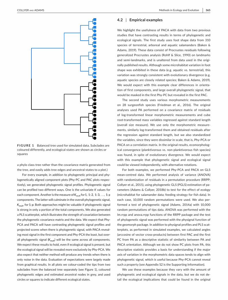
We simulated a balanced tree (Figure 1) with 25 tips (five sub-clade levels) using the stree function of the ape R package, version 5.3 (Paradis & Schliep, 2018). To simulate P and R, we used the sim.char function of the geiger r package, version 2.0.6.2 (Harmon et al., 2008), which simulates Y=P+R for an input tree. We pro-duced matrices of p = 10 variables with R simulated from a multivar-iate normal distribution with � equal to a vector of p = 10 0s and Σ equal to 1Ip×p. (Adding correlation structure had no qualitative effect on results; see Appendix S3 in the Supporting Information.) For simu-lations including ecological signal, every other row of E was assigned values of 1.5 rather than 0, which had the effect of shifting means for one tip from pairs of tips in the balanced tree. R scripts with an-notations for these data simulations are provided in Appendix S2 of the Supporting Information. All simulated data and any subsequent simulated data or analyses were performed in version 4.0.2 of R (R Core Team, 2019). All Phy-PCA and PACA analyses, here and subse-quently, were performed with a combination of the ordinate func-tion in the RRPP package, version 0.6.1.900 (Collyer & Adams, 2018) and the gm.prcomp function in the geomorph package, version 3.3.1 (Adams et al., 2020; Adams & Otárola-Castillo, 2013). (The latter function is a wrapper of the former function, which allows input of

     |  365Methods in Ecology and Evolu onCOLLYER and adaMS

a phylo class tree rather than the covariance matrix generated from the tree, and easily adds tree edges and ancestral states to a plot.)

For every example, in addition to phylogenetic principal and phy-logenetically aligned component plots (Phy-PC and PAC plots respec-tively), we generated phylogenetic signal profiles. Phylogenetic signal can be profiled two different ways. One is the univariate K values for each component. Another is the measure of Kmult for 1, 1: 2, 1: 3, …, 1: p components. The latter will culminate in the overall phylogenetic signal, Kmult, for 1: p. Both approaches might be valuable if phylogenetic signal is strong in only a portion of the total components. We also generated a PLS scatterplot, which illustrates the strength of covariation between the phylogenetic covariance matrix and the data. We expect that Phy-PCA and PACA will have contrasting phylogenetic signal profiles and projected scores when there is phylogenetic signal, with PACA reveal-ing most signal in the first component and Phy-PCA the least, but over-all phylogenetic signal (Kmult) will be the same across all components. We expect these results to hold, even if ecological signal is present, but the ecological signal will be revealed more exclusively by Phy-PCA. We also expect that neither method will produce any trends when there is only noise in the data. Evaluation of expectations were largely made from graphical results. In all plots we colour-coded the tips from two subclades from the balanced tree separately (see Figure 1), coloured phylogenetic edges and estimated ancestral nodes in grey, and used circles or squares to indicate different ecological states.

4.2 | Empirical examples

We highlight the usefulness of PACA with data from two previous studies that have contrasting results in terms of phylogenetic and ecological signals. The first study uses foot shape data from 310 species of terrestrial, arboreal and aquatic salamanders (Baken & Adams, 2019). These data consist of Procrustes residuals following generalized Procrustes analysis (Rohlf & Slice, 1990) on landmarks and semi-landmarks, and is unaltered from data used in the origi-nally published results. Although some microhabitat variation in foot shape was exhibited in these data (e.g. aquatic vs. terrestrial), this variation was strongly consistent with evolutionary divergence (e.g. aquatic species are closely related species; Baken & Adams, 2019). We would expect with this example clear differences in orienta-tion of first components, and large overall phylogenetic signal, that would be masked in the first Phy-PC but revealed in the first PAC.

The second study uses various morphometric measurements on 28 surgeonfish species (Friedman et al., 2016). The original analyses used PA performed on a covariance matrix of residuals of log-transformed linear morphometric measurements and cube root-transformed mass variables regressed against standard length (overall size measure). We use only the morphometric measure-ments, similarly log-transformed them and obtained residuals after the regression against standard length, but we also standardized the variables, since they were dissimilar in scale, that is, Phy-PCA or PACA on a correlation matrix. In the original results, ecomorpholog-ical convergence (planktivorous vs. non-planktivorous fish species) was found, in spite of evolutionary divergence. We would expect with this example that phylogenetic signal and ecological signal could be viewed independently, with alternative rotations.

For both examples, we performed Phy-PCA and PACA on GLS mean-centred data. We performed analysis of variance (ANOVA) with randomization of residuals in a permutation procedure (RRPP; Collyer et al., 2015), using phylogenetic GLS (PGLS) estimation of pa-rameters (Adams & Collyer, 2018b) to test for the effect of ecology (microhabitat for salamander data; feeding strategy for fish data). In each case, 10,000 random permutations were used. We also per-formed a test of phylogenetic signal (Adams, 2014a) with 10,000 random permutations of tips data. ANOVA was performed with the lm.rrpp and anova.rrpp functions of the RRPP package and the test of phylogenetic signal was performed with the physignal function of the geomorph package. In addition to physignal profiles and PLS scat-terplots, as performed in simulated examples, we calculated angles (arccosine of vector cross-products) between first PAC and the first PC from PA as a descriptive statistic of similarity between PA and PACA orientation. Although we do not show PC plots from PA, this descriptive statistic provides a basis for understanding if the major axis of variation in the morphometric data spaces tends to align with phylogenetic signal, which is useful because Phy-PCA cannot reveal such a property (see Appendix S2 is the Supporting Information).

We use these examples because they vary with the amount of phylogenetic and ecological signals in the data, but we do not de-tail the ecological implications that could be found in the original

F I G U R E 1   Balanced tree used for simulated data. Subclades are coloured differently, and ecological states are shown as circles or squares

366  |    Methods in Ecology and Evolu on COLLYER and adaMS

sources. For example, we do not provide visual representation of foot shape changes in the ordination plots, which are shown in Baken and Adams (2019). Our focus is on how the different ordinations re-late to each other, given different ecological signals in the data.

5  | RESULTS

5.1 | Simulated examples

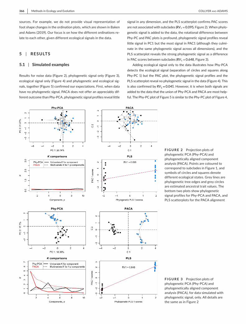
Results for noise data (Figure 2), phylogenetic signal only (Figure 3), ecological signal only (Figure 4) and phylogenetic and ecological sig-nals, together (Figure 5) confirmed our expectations. First, when data have no phylogenetic signal, PACA does not offer an appreciably dif-ferent outcome than Phy-PCA, phylogenetic signal profiles reveal little

signal in any dimension, and the PLS scatterplot confirms PAC scores are not associated with subclades (RV1=0.095, Figure 2). When phylo-genetic signal is added to the data, the rotational difference between Phy-PC and PAC plots is profound, phylogenetic signal profiles reveal little signal in PC1 but the most signal in PAC1 (although they culmi-nate in the same phylogenetic signal across all dimensions), and the PLS scatterplot reveals the strong phylogenetic signal as a difference in PAC scores between subclades (RV1=0.648, Figure 3).

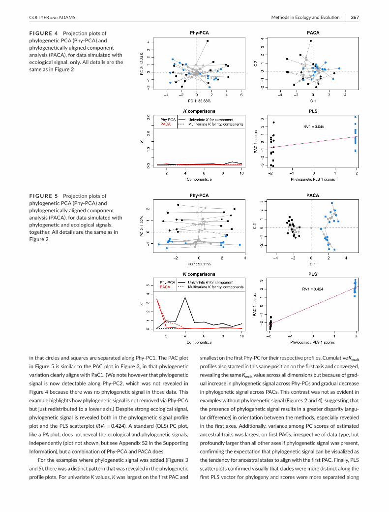
Adding ecological signal only to the data illustrates how Phy-PCA detects the ecological signal (separation of circles and squares along Phy-PC 1) but the PAC plot, the phylogenetic signal profiles and the PLS scatterplot reveal no phylogenetic signal in the data (Figure 4). This is also confirmed by RV1=0.045. However, it is when both signals are added to the data that the union of Phy-PCA and PACA are most help-ful. The Phy-PC plot of Figure 5 is similar to the Phy-PC plot of Figure 4,

F I G U R E 2   Projection plots of phylogenetic PCA (Phy-PCA) and phylogenetically aligned component analysis (PACA). Points are coloured to correspond to subclades in Figure 1, and symbols of circles and squares denote different ecological states. Grey lines are phylogenetic tree edges and grey circles are estimated ancestral trait values. The bottom two plots show phylogenetic signal profiles for Phy-PCA and PACA, and PLS scatterplots for the PACA alignment

F I G U R E 3   Projection plots of phylogenetic PCA (Phy-PCA) and phylogenetically aligned component analysis (PACA), for data simulated with phylogenetic signal, only. All details are the same as in Figure 2

     |  367Methods in Ecology and Evolu onCOLLYER and adaMS

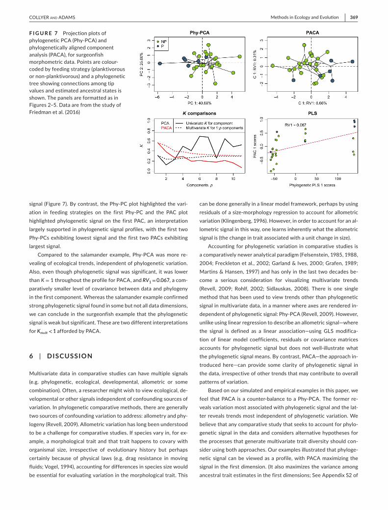
in that circles and squares are separated along Phy-PC1. The PAC plot in Figure 5 is similar to the PAC plot in Figure 3, in that phylogenetic variation clearly aligns with PaC1. (We note however that phylogenetic signal is now detectable along Phy-PC2, which was not revealed in Figure 4 because there was no phylogenetic signal in those data. This example highlights how phylogenetic signal is not removed via Phy-PCA but just redistributed to a lower axis.) Despite strong ecological signal, phylogenetic signal is revealed both in the phylogenetic signal profile plot and the PLS scatterplot (RV1=0.424). A standard (OLS) PC plot, like a PA plot, does not reveal the ecological and phylogenetic signals, independently (plot not shown, but see Appendix S2 in the Supporting Information), but a combination of Phy-PCA and PACA does.

For the examples where phylogenetic signal was added (Figures 3 and 5), there was a distinct pattern that was revealed in the phylogenetic profile plots. For univariate K values, K was largest on the first PAC and

smallest on the first Phy-PC for their respective profiles. Cumulative Kmult profiles also started in this same position on the first axis and converged, revealing the same Kmult value across all dimensions but because of grad-ual increase in phylogenetic signal across Phy-PCs and gradual decrease in phylogenetic signal across PACs. This contrast was not as evident in examples without phylogenetic signal (Figures 2 and 4), suggesting that the presence of phylogenetic signal results in a greater disparity (angu-lar difference) in orientation between the methods, especially revealed in the first axes. Additionally, variance among PC scores of estimated ancestral traits was largest on first PACs, irrespective of data type, but profoundly larger than all other axes if phylogenetic signal was present, confirming the expectation that phylogenetic signal can be visualized as the tendency for ancestral states to align with the first PAC. Finally, PLS scatterplots confirmed visually that clades were more distinct along the first PLS vector for phylogeny and scores were more separated along

F I G U R E 4   Projection plots of phylogenetic PCA (Phy-PCA) and phylogenetically aligned component analysis (PACA), for data simulated with ecological signal, only. All details are the same as in Figure 2

F I G U R E 5   Projection plots of phylogenetic PCA (Phy-PCA) and phylogenetically aligned component analysis (PACA), for data simulated with phylogenetic and ecological signals, together. All details are the same as in Figure 2

368  |    Methods in Ecology and Evolu on COLLYER and adaMS

the first PAC, compared to examples without phylogenetic signal. The slopes of best fit lines in these plots corresponded to RV1 values.

What these results illustrate, comprehensively, is that the com-bination of Phy-PCA and PACA allows one to visualize trends inde-pendent of and focused on phylogenetic signal respectively. We also performed additional simulation runs (100 per set) with the same con-ditions, plus varied the number of taxa, the number of variables, the relative strength of phylogenetic and ecological signals, and the cor-relation among variables. These results are provided in Appendix S3 of the Supporting Information. In general, the same results were found despite varying parameters, with three exceptions. First, increasing the amount of ecological signal relative to phylogenetic signal reduced slightly both RV1 and K1 in the first phylogenetically aligned compo-nent, but phylogenetic signal was still substantially larger in the first component compared to Phy-PCA. This result makes sense if—like in our simulations—ecological and phylogenetic signals are not cor-related. Second, increased variable correlations mitigated RV1 and K1

, but only slightly. However, we confirmed in such cases that overall RV and Kmult tended to be similar, suggesting that variable correlations influence the distribution of phylogenetic signal across components more so than the amount of phylogenetic signal, overall. Finally, in-creased tree depth (tree size) very slightly reduced the median value of RV1, suggesting that tree size and phylogenetic signal are intrinsically related. In these three cases, the trends were practically negligible compared to the contrast in results between Phy-PCA and PACA. The number of variables had no apparent effect on RV1 and K1, and none of the varied parameters seemed to obfuscate PACA's ability to visualize the maximum phylogenetic signal in the data.

5.2 | Empirical examples

The salamander foot shape data did not have a significant ecological (microhabitat) signal (RRPP-ANOVA: Z = 0.97174; p = 0.1609) but had a significant phylogenetic signal (multivariate Kmult=0.90498;

Z = 16.03612; p = 0.0001). The angle between the first components was 4.544°, indicating that PACs were aligned similar to PCs (from PA, not Phy-PCA) and that phylogenetic signal largely accounted for the major axis of variation in the multivariate data space. The Kmult was less than 1, however, suggesting that phylogenetic signal is weaker than expected with a BM model of evolutionary divergence, despite the large effect size. Nonetheless, K on the first component, K1, was quite large (2.7566), suggesting that Kmult=0.90498 is not a weak phylogenetic signal but rather that the signal was concentrated in some but not all variables of the original data (Figure 6). The Phy-PCA was orientated differently, with the variation along the first PAC largely represented along the second Phy-PC (Figure 6). This was confirmed with phylogenetic signal profiles, with most phylo-genetic signal on the first PAC and comparatively less phylogenetic signal on the first Phy-PC, but nearly as much phylogenetic signal on the second Phy-PC as the first PAC.

These results highlight how PACA specifically aligns with phy-logenetic signal in its first component and Phy-PCA finds a first component that is mostly independent of phylogenetic signal. Interestingly, the first Phy-PC is not the component with the low-est phylogenetic signal, having a K of 0.6054, which is larger than all other components except three (Figure 6). Additionally, although Phy-PCs are orientated quite differently than PACs, the small effect size of microhabitat suggests that Phy-PCA is not necessarily show-ing a better representation of ecological variation, independent of phylogeny. This is especially not possible in this case because micro-habitat types are largely clustered within some subclades (Figure 6). Thus, PACA provides a more meaningful ordination plot than Phy-PCA, in this particular case.

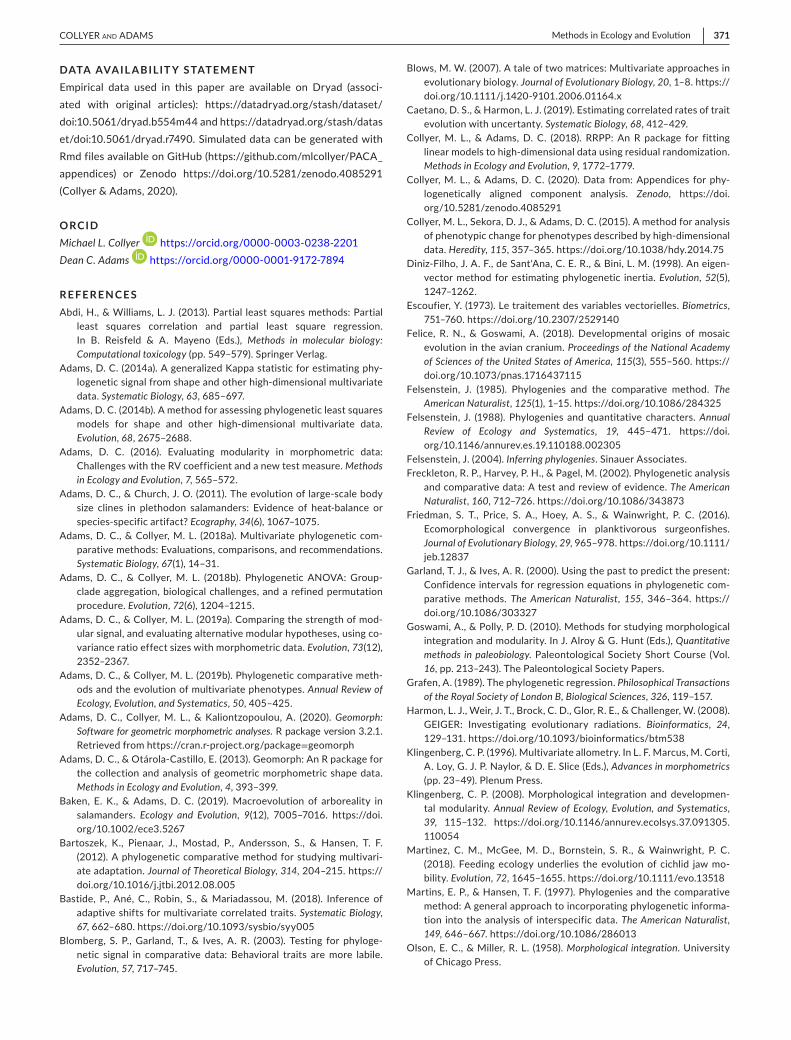
The surgeonfish data had a significant ecological (feeding strat-egy) signal (RRPP-ANOVA: Z = 2.6553; p = 0.0007) and a significant phylogenetic signal (Kmult=0.35305; Z = 2.29545; p = 0.0023). The angle between the first components was 37.534°, indicating that PACs were not aligned similar to PCs (from PA, not Phy-PCA) and that a PC plot would not be orientated strongly with phylogenetic

F I G U R E 6   Projection plots of phylogenetic PCA (Phy-PCA) and phylogenetically aligned component analysis (PACA), for salamander foot shape data. Points are colour-coded by microhabitat and a phylogenetic tree showing connections among tip values and estimated ancestral states is shown. The panels are formatted as in Figures 2–5. Microhabitats include saxicolous (S), arboreal (A), terrestrial (T), aquatic/water (W), cave (C) and fossorial (F). Data are from the study of Baken and Adams (2019)

     |  369Methods in Ecology and Evolu onCOLLYER and adaMS

signal (Figure 7). By contrast, the Phy-PC plot highlighted the vari-ation in feeding strategies on the first Phy-PC and the PAC plot highlighted phylogenetic signal on the first PAC, an interpretation largely supported in phylogenetic signal profiles, with the first two Phy-PCs exhibiting lowest signal and the first two PACs exhibiting largest signal.

Compared to the salamander example, Phy-PCA was more re-vealing of ecological trends, independent of phylogenetic variation. Also, even though phylogenetic signal was significant, it was lower than K = 1 throughout the profile for PACA, and RV1=0.067, a com-paratively smaller level of covariance between data and phylogeny in the first component. Whereas the salamander example confirmed strong phylogenetic signal found in some but not all data dimensions, we can conclude in the surgeonfish example that the phylogenetic signal is weak but significant. These are two different interpretations for Kmult<1 afforded by PACA.

6  | DISCUSSION

Multivariate data in comparative studies can have multiple signals (e.g. phylogenetic, ecological, developmental, allometric or some combination). Often, a researcher might wish to view ecological, de-velopmental or other signals independent of confounding sources of variation. In phylogenetic comparative methods, there are generally two sources of confounding variation to address: allometry and phy-logeny (Revell, 2009). Allometric variation has long been understood to be a challenge for comparative studies. If species vary in, for ex-ample, a morphological trait and that trait happens to covary with organismal size, irrespective of evolutionary history but perhaps certainly because of physical laws (e.g. drag resistance in moving fluids; Vogel, 1994), accounting for differences in species size would be essential for evaluating variation in the morphological trait. This

can be done generally in a linear model framework, perhaps by using residuals of a size-morphology regression to account for allometric variation (Klingenberg, 1996). However, in order to account for an al-lometric signal in this way, one learns inherently what the allometric signal is (the change in trait associated with a unit change in size).

Accounting for phylogenetic variation in comparative studies is a comparatively newer analytical paradigm (Felsenstein, 1985, 1988, 2004; Freckleton et al., 2002; Garland & Ives, 2000; Grafen, 1989; Martins & Hansen, 1997) and has only in the last two decades be-come a serious consideration for visualizing multivariate trends (Revell, 2009; Rohlf, 2002; Sidlauskas, 2008). There is one single method that has been used to view trends other than phylogenetic signal in multivariate data, in a manner where axes are rendered in-dependent of phylogenetic signal: Phy-PCA (Revell, 2009). However, unlike using linear regression to describe an allometric signal—where the signal is defined as a linear association—using GLS modifica-tion of linear model coefficients, residuals or covariance matrices accounts for phylogenetic signal but does not well-illustrate what the phylogenetic signal means. By contrast, PACA—the approach in-troduced here—can provide some clarity of phylogenetic signal in the data, irrespective of other trends that may contribute to overall patterns of variation.

Based on our simulated and empirical examples in this paper, we feel that PACA is a counter-balance to a Phy-PCA. The former re-veals variation most associated with phylogenetic signal and the lat-ter reveals trends most independent of phylogenetic variation. We believe that any comparative study that seeks to account for phylo-genetic signal in the data and considers alternative hypotheses for the processes that generate multivariate trait diversity should con-sider using both approaches. Our examples illustrated that phyloge-netic signal can be viewed as a profile, with PACA maximizing the signal in the first dimension. (It also maximizes the variance among ancestral trait estimates in the first dimensions; See Appendix S2 of

F I G U R E 7   Projection plots of phylogenetic PCA (Phy-PCA) and phylogenetically aligned component analysis (PACA), for surgeonfish morphometric data. Points are colour-coded by feeding strategy (planktivorous or non-planktivorous) and a phylogenetic tree showing connections among tip values and estimated ancestral states is shown. The panels are formatted as in Figures 2–5. Data are from the study of Friedman et al. (2016)

370  |    Methods in Ecology and Evolu on COLLYER and adaMS

the Supporting Information.) Many studies that test for phylogenetic signal might report ‘significant but weak’ signal, whereby a hypoth-esis test confirms that similar taxa have more similar traits, as ex-pected with a Brownian motion model of evolutionary divergence, but the generalized Kmult value is considerably <1 (for a review see: Adams & Collyer, 2019b). We could make the same conclusions with the empirical examples we used to illustrate PACA. Both had gen-eralized Kmult values <1 that were significant. However, in the sala-mander example, the K value of the first component was large, that is, K>2. Comparatively, the surgeonfish example had a much smaller K1=0.553. We believe that these contrasting examples show in one case, a very large and significant phylogenetic signal especially in some latent dimensions of the full data space (salamanders) and a weak but significant phylogenetic signal more diffusely in the data (surgeonfish). By rotating the data space to the axis of greatest phy-logenetic signal with PACA, one can discern between such different conclusions that manifest similarly in a hypothesis test, especially for highly multivariate data.

Similarly, one can measure the component by component strength of association of data with phylogeny by the partial RV scores. Researchers are generally comfortable with interpreting the portion of total variation explained by PC axes as a proxy for the strength of a trend that shown in a plot of projected PC scores. For example, if the first PC explains a rather large portion of the overall variation, one might feel that, for example, morphological change along that axis could represent a valid biological phenom-enon. The partial RV scores—summing to the total RV rather than 1—relay the importance of evolutionary history as a diversification trend, especially along the first phylogenetically aligned compo-nent. For the salamander example, this trend was strong, so much so that PAC and PA plots were quite similar in orientation. In the surgeonfish example, this trend was weaker, as morphological variation was also associated with feeding strategy, and planktiv-orous fish could be expected to have some common morphologi-cal features, irrespective of evolutionary history. We also showed that if we replace a phylogenetic covariance matrix with an iden-tity matrix, partial RV was a generalization that simplified to partial variance explained by axes (if the axes were principal). Therefore, partial RV values should have some natural appeal for researchers who are used to PCA.

Although PACA reveals an orientation of a data space that maxi-mizes phylogenetic signal in the first few components, we do not ad-vocate a reduction of data to the first few dimensions of PAC scores as a surrogate for the entire multivariate dataset, for the purpose of using multivariate analyses that are constrained by variable number. This has been shown to be a foolhardy practice with PC scores, as a bias for more complex models of evolutionary divergence is garnered by using only a few PCs on data simulated from a BM process (Uyeda et al., 2015). We do not suspect that PACA could alleviate a data reduction travesty. Furthermore, because a phylogenetic covariance matrix assumes a BM model of evolutionary divergence—the precise model for phylogenetic signal estimation—PACA results should not suggest an alternative model of evolutionary divergence in the first

few PACs but the opposite problem would be likely; aligning data to a covariance matrix based on a model of BM evolutionary diver-gence might obfuscate interpretations about the most likely model of evolutionary divergence because of the constraint of maximizing (BM) phylogenetic signal in the process, if only a few dimensions are considered. Like Uyeda et al. (2015) we believe inferences made among competing models of evolutionary divergence have to use all data dimensions, but if all PAC scores are used, then the inferences should be the same as with the original data, provided the methods used are rotation-invariant in model likelihood estimation (Adams & Collyer, 2018a, 2019b).

Evolutionary biologists widely recognize that phenotypic evo-lution occurs multivariately (Adams & Collyer, 2018a, 2019b; Blows, 2007; Collyer et al., 2015), where sets of traits, as well as the dimensions of complex multivariate traits, evolve in a correlated fash-ion across the tree of life in response to ecological selective forces. Visualizing evolutionary changes in such spaces requires ordination approaches that are capable of capturing these patterns, ideally in a manner that facilitates biological interpretation of the putative pro-cesses that have generated them. Phylogenetically aligned compo-nents analysis provides one such approach. PACA aligns multivariate variation in trait data with phylogenetic signal, and thus is capable of revealing whether phylogenetic signal is intensified in fewer data dimensions, or more diffusely distributed across all data dimensions. As with all ordination approaches, PACA is a descriptive tool, but one that should have nice association with tests of phylogenetic sig-nal. Our simulated and empirical examples demonstrate the utility of the approach, and how it differs from Phy-PCA. Importantly, in comparative studies that seek to disentangle phylogenetic and other (ecological) sources of multivariate trait variation, a combination of PACA and Phy-PCA should make such an objective possible. Thus, PACA provides an important analytical tool in the repertoire of the phylogenetic comparative biologist for studying macroevolutionary trends in multivariate phenotypes.

ACKNOWLEDG EMENTSThis work was sponsored in part by National Science Foundation Grants DBI-1902694 (to M.L.C.) and DBI-1902511 (to D.C.A.). The authors appreciate the enthusiasm from E. Baken and S. Friedman for including data from their research as examples. This paper ben-efited substantially from the comments of three anonymous review-ers. The authors have no known conflict of interest.

AUTHORS' CONTRIBUTIONSM.L.C. conceived the original idea for this manuscript, and both M.L.C. and D.C.A. collaboratively developed the concept and con-tributed to all portions of this manuscript. Both the authors approve of the final product and are willingly accountable for any portion of the content.

PEER RE VIE WThe peer review history for this article is available at https://publo ns. com/publo n/10.1111/2041-210X.13515.

     |  371Methods in Ecology and Evolu onCOLLYER and adaMS

DATA AVAIL ABILIT Y S TATEMENTEmpirical data used in this paper are available on Dryad (associ-ated with original articles): https://datad ryad.org/stash/ datas et/doi:10.5061/dryad.b554m44 and https://datad ryad.org/stash/ datas et/doi:10.5061/dryad.r7490. Simulated data can be generated with Rmd files available on GitHub (https://github.com/mlcol lyer/PACA_appen dices) or Zenodo https://doi.org/10.5281/zenodo.4085291 (Collyer & Adams, 2020).

ORCIDMichael L. Collyer https://orcid.org/0000-0003-0238-2201 Dean C. Adams https://orcid.org/0000-0001-9172-7894

R E FE R E N C E SAbdi, H., & Williams, L. J. (2013). Partial least squares methods: Partial

least squares correlation and partial least square regression. In B. Reisfeld & A. Mayeno (Eds.), Methods in molecular biology: Computational toxicology (pp. 549–579). Springer Verlag.

Adams, D. C. (2014a). A generalized Kappa statistic for estimating phy-logenetic signal from shape and other high-dimensional multivariate data. Systematic Biology, 63, 685–697.

Adams, D. C. (2014b). A method for assessing phylogenetic least squares models for shape and other high-dimensional multivariate data. Evolution, 68, 2675–2688.

Adams, D. C. (2016). Evaluating modularity in morphometric data: Challenges with the RV coefficient and a new test measure. Methods in Ecology and Evolution, 7, 565–572.

Adams, D. C., & Church, J. O. (2011). The evolution of large-scale body size clines in plethodon salamanders: Evidence of heat-balance or species-specific artifact? Ecography, 34(6), 1067–1075.

Adams, D. C., & Collyer, M. L. (2018a). Multivariate phylogenetic com-parative methods: Evaluations, comparisons, and recommendations. Systematic Biology, 67(1), 14–31.

Adams, D. C., & Collyer, M. L. (2018b). Phylogenetic ANOVA: Group-clade aggregation, biological challenges, and a refined permutation procedure. Evolution, 72(6), 1204–1215.

Adams, D. C., & Collyer, M. L. (2019a). Comparing the strength of mod-ular signal, and evaluating alternative modular hypotheses, using co-variance ratio effect sizes with morphometric data. Evolution, 73(12), 2352–2367.

Adams, D. C., & Collyer, M. L. (2019b). Phylogenetic comparative meth-ods and the evolution of multivariate phenotypes. Annual Review of Ecology, Evolution, and Systematics, 50, 405–425.

Adams, D. C., Collyer, M. L., & Kaliontzopoulou, A. (2020). Geomorph: Software for geometric morphometric analyses. R package version 3.2.1. Retrieved from https://cran.r-proje ct.org/packa ge=geomorph

Adams, D. C., & Otárola-Castillo, E. (2013). Geomorph: An R package for the collection and analysis of geometric morphometric shape data. Methods in Ecology and Evolution, 4, 393–399.

Baken, E. K., & Adams, D. C. (2019). Macroevolution of arboreality in salamanders. Ecology and Evolution, 9(12), 7005–7016. https://doi.org/10.1002/ece3.5267

Bartoszek, K., Pienaar, J., Mostad, P., Andersson, S., & Hansen, T. F. (2012). A phylogenetic comparative method for studying multivari-ate adaptation. Journal of Theoretical Biology, 314, 204–215. https://doi.org/10.1016/j.jtbi.2012.08.005

Bastide, P., Ané, C., Robin, S., & Mariadassou, M. (2018). Inference of adaptive shifts for multivariate correlated traits. Systematic Biology, 67, 662–680. https://doi.org/10.1093/sysbi o/syy005

Blomberg, S. P., Garland, T., & Ives, A. R. (2003). Testing for phyloge-netic signal in comparative data: Behavioral traits are more labile. Evolution, 57, 717–745.

Blows, M. W. (2007). A tale of two matrices: Multivariate approaches in evolutionary biology. Journal of Evolutionary Biology, 20, 1–8. https://doi.org/10.1111/j.1420-9101.2006.01164.x

Caetano, D. S., & Harmon, L. J. (2019). Estimating correlated rates of trait evolution with uncertanty. Systematic Biology, 68, 412–429.

Collyer, M. L., & Adams, D. C. (2018). RRPP: An R package for fitting linear models to high-dimensional data using residual randomization. Methods in Ecology and Evolution, 9, 1772–1779.

Collyer, M. L., & Adams, D. C. (2020). Data from: Appendices for phy-logenetically aligned component analysis. Zenodo, https://doi.org/10.5281/zenodo.4085291

Collyer, M. L., Sekora, D. J., & Adams, D. C. (2015). A method for analysis of phenotypic change for phenotypes described by high-dimensional data. Heredity, 115, 357–365. https://doi.org/10.1038/hdy.2014.75

Diniz-Filho, J. A. F., de Sant'Ana, C. E. R., & Bini, L. M. (1998). An eigen-vector method for estimating phylogenetic inertia. Evolution, 52(5), 1247–1262.

Escoufier, Y. (1973). Le traitement des variables vectorielles. Biometrics, 751–760. https://doi.org/10.2307/2529140

Felice, R. N., & Goswami, A. (2018). Developmental origins of mosaic evolution in the avian cranium. Proceedings of the National Academy of Sciences of the United States of America, 115(3), 555–560. https://doi.org/10.1073/pnas.17164 37115

Felsenstein, J. (1985). Phylogenies and the comparative method. The American Naturalist, 125(1), 1–15. https://doi.org/10.1086/284325

Felsenstein, J. (1988). Phylogenies and quantitative characters. Annual Review of Ecology and Systematics, 19, 445–471. https://doi.org/10.1146/annur ev.es.19.110188.002305

Felsenstein, J. (2004). Inferring phylogenies. Sinauer Associates.Freckleton, R. P., Harvey, P. H., & Pagel, M. (2002). Phylogenetic analysis

and comparative data: A test and review of evidence. The American Naturalist, 160, 712–726. https://doi.org/10.1086/343873

Friedman, S. T., Price, S. A., Hoey, A. S., & Wainwright, P. C. (2016). Ecomorphological convergence in planktivorous surgeonfishes. Journal of Evolutionary Biology, 29, 965–978. https://doi.org/10.1111/jeb.12837

Garland, T. J., & Ives, A. R. (2000). Using the past to predict the present: Confidence intervals for regression equations in phylogenetic com-parative methods. The American Naturalist, 155, 346–364. https://doi.org/10.1086/303327

Goswami, A., & Polly, P. D. (2010). Methods for studying morphological integration and modularity. In J. Alroy & G. Hunt (Eds.), Quantitative methods in paleobiology. Paleontological Society Short Course (Vol. 16, pp. 213–243). The Paleontological Society Papers.

Grafen, A. (1989). The phylogenetic regression. Philosophical Transactions of the Royal Society of London B, Biological Sciences, 326, 119–157.

Harmon, L. J., Weir, J. T., Brock, C. D., Glor, R. E., & Challenger, W. (2008). GEIGER: Investigating evolutionary radiations. Bioinformatics, 24, 129–131. https://doi.org/10.1093/bioin forma tics/btm538

Klingenberg, C. P. (1996). Multivariate allometry. In L. F. Marcus, M. Corti, A. Loy, G. J. P. Naylor, & D. E. Slice (Eds.), Advances in morphometrics (pp. 23–49). Plenum Press.

Klingenberg, C. P. (2008). Morphological integration and developmen-tal modularity. Annual Review of Ecology, Evolution, and Systematics, 39, 115–132. https://doi.org/10.1146/annur ev.ecols ys.37.091305. 110054

Martinez, C. M., McGee, M. D., Bornstein, S. R., & Wainwright, P. C. (2018). Feeding ecology underlies the evolution of cichlid jaw mo-bility. Evolution, 72, 1645–1655. https://doi.org/10.1111/evo.13518

Martins, E. P., & Hansen, T. F. (1997). Phylogenies and the comparative method: A general approach to incorporating phylogenetic informa-tion into the analysis of interspecific data. The American Naturalist, 149, 646–667. https://doi.org/10.1086/286013

Olson, E. C., & Miller, R. L. (1958). Morphological integration. University of Chicago Press.

372  |    Methods in Ecology and Evolu on COLLYER and adaMS

Paradis, E., & Schliep, K. (2018). Ape 5.0: An environment for modern phylogenetics and evolutionary analyses in R. Bioinformatics, 35, 526–528.

Polly, P. D., Lawing, A. M., Fabre, A., & Goswami, A. (2013). Phylogenetic principal components analysis and geometric morphometrics. Hystrix, 24, 33–41.

Price, S. A., Wainwright, P. C., Bellwood, D. R., Kazancioglu, E., Collar, D. C., & Near, T. J. (2010). Functional innovations and morphological diversification in parrotfish. Evolution, 64, 3057–3068. https://doi.org/10.1111/j.1558-5646.2010.01036.x

R Core Team. (2019). R: A language and environment for statistical comput-ing. R Foundation for Statistical Computing. Retrieved from https://www.R-proje ct.org/

Revell, L. J. (2009). Size-correction and principal components for inter-specific comparative studies. Evolution, 63, 3258–3268. https://doi.org/10.1111/j.1558-5646.2009.00804.x

Revell, L. J., & Harmon, L. J. (2008). Testing quantitative genetic hypoth-eses about the evolutionary rate matrix for continuous characters. Evolutionary Ecology Research, 10, 311–331.

Rohlf, F. J. (2001). Comparative methods for the analysis of continuous variables: Geometric interpretations. Evolution, 55(11), 2143–2160.

Rohlf, F. J. (2002). Geometric morphometrics and phylogeny. In N. MacLeod & P. L. Forey (Eds.), Morphology, shape and phylogeny (pp. 175–193). Taylor & Francis.

Rohlf, F. J., & Corti, M. (2000). The use of partial least-squares to study covariation in shape. Systematic Biology, 49, 740–753.

Rohlf, F. J., & Slice, D. E. (1990). Extensions of the procrustes method for the optimal superimposition of landmarks. Systematic Zoology, 39, 40–59. https://doi.org/10.2307/2992207

Sherratt, E., Alejandrino, A., Kraemer, A. C., Serb, J. M., & Adams, D. C. (2016). Trends in the sand: Directional evolution in the shell shape of recessing scallops (Bivalvia: Pectinidae). Evolution, 70, 2061–2073. https://doi.org/10.1111/evo.12995

Sidlauskas, B. (2008). Continuous and arrested morphological di-versification in sister clades of characiform fishes: A phylo-morphospace approach. Evolution, 62, 3135–3156. https://doi.org/10.1111/j.1558-5646.2008.00519.x

Uyeda, J. C., Caetano, D. S., & Pennell, M. W. (2015). Comparative anal-ysis of principal components can be misleading. Systematic Biology, 64(4), 677–689. https://doi.org/10.1093/sysbi o/syv019

Vaux, F., Trewick, S. A., Crampton, J. S., Marshall, B. A., Beu, A. G., Hills, S. F., & Morgan-Richards, M. (2018). Evolutionary lineages of ma-rine snails identified using molecular phylogenetics and geomet-ric morphometric analysis of shells. Molecular Phylogenetics and Evolution, 127, 626–637. https://doi.org/10.1016/j.ympev.2018. 06.009

Vogel, S. (1994). Life in moving fluids: The physical biology of flow. Princeton University Press.

Zelditch, M. L., Ye, J., Mitchell, J. S., & Swiderski, D. L. (2017). Rare eco-morphological convergence on a complex adaptive landscape: Body size and diet mediate evolution of jaw shape in squirrels (Sciuridae). Evolution, 71, 633–649. https://doi.org/10.1111/evo.13168

SUPPORTING INFORMATIONAdditional supporting information may be found online in the Supporting Information section.

How to cite this article: Collyer ML, Adams DC. Phylogenetically aligned component analysis. Methods Ecol Evol. 2021;12:359–372. https://doi.org/10.1111/2041-210X.13515