© The Norwegian Academy of Science and Letters 2005 • Zoologica Scripta, 34, 5, September 2005, pp447– 468 447 Stockley, B., Smith, A. B., Littlewood T., Lessios H. A. & MacKenzie-Dodds J. A. (2005). Phylo- genetic relationships of spatangoid sea urchins (Echinoidea): taxon sampling density and congruence between morphological and molecular estimates. — Zoologica Scripta, 34, 447– 468. A phylogeny for 21 species of spatangoid sea urchins is constructed using data from three genes and results compared with morphology-based phylogenies derived for the same taxa and for a much larger sample of 88 Recent and fossil taxa. Different data sets and methods of analysis generate different phylogenetic hypotheses, although congruence tests show that all molecular approaches produce trees that are congruent with each other. By contrast, the trees generated from morphological data differ significantly according to taxon sampling density and only those with dense sampling (after a posteriori weighting) are congruent with molecular estimates. With limited taxon sampling, secondary reversals in deep-water taxa are interpreted as plesiomorphies, pulling them to a basal position. The addition of fossil taxa with their unique character combinations reveals hidden homoplasy and generates a phylogeny that is compatible with molecular estimates. As homoplasy levels were found to be broadly similar across different anatomical structures in the echinoid test, no one suite of morphological characters can be considered to provide more reliable phylogenetic information. Some traditional groupings are supported, including the grouping of Loveniidae, Brissidae and Spatangidae within the Micrasterina, but the Asterostomatidae is shown to be polyphyletic with members scattered amongst at least five different clades. As these are mostly deep-sea taxa, this finding implies multiple independent invasions into the deep sea. Bruce Stockley, Andrew Smith, Tim Littlewood, Jacqueline A. MacKenzie-Dodds, The Natural History Museum, Cromwell Road, London SW67 5BD, UK. E-mail: [email protected] Harilaos Lessios, Smithsonian Tropical Research Institute, Balboa, Panama. E-mail: [email protected] Blackwell Publishing, Ltd. Phylogenetic relationships of spatangoid sea urchins (Echinoidea): taxon sampling density and congruence between morphological and molecular estimates BRUCE STOCKLEY, ANDREW B. SMITH, TIM LITTLEWOOD, HARILAOS A. LESSIOS & JACQUELINE A. MACKENZIE-DODDS Accepted: 13 April 2005 doi:10.1111/j.1463-6409.2005.00201.x Introduction The combined use of morphological and molecular data to investigate phylogenetic relationships is now standard practice, with data from the two sources usually being kept separate at least initially for comparative purposes (De Queiroz et al 1995). In many cases the two data sets provide compatible (though rarely identical) topologies, and the two can safely be combined. How- ever, data sets drawn from multiple genes or from morphology and molecular sources are sometimes so different that there is no justification for treating them as suboptimal estimates of the same underlying topology (see Larson 1994; Farris et al . 1994; Cunningham 1997). A decision has then to be made as to which is more likely to be in error. The causes of significant mismatch between independent data sets are thus usually attributed to biases inherent in the data rather than to inadequate sampling (either of characters or taxa). A number of parallel molecular and morphological studies of echinoderms have been carried out, focusing on the relationships of the five classes (e.g. Littlewood et al . 1997; Janies 2001; Smith et al . 2004), or on relationships within the individual classes (e.g. Smith et al . 1995a,b; Littlewood & Smith 1995; Lafay et al . 1995; Kerr & Kim 2001; Jeffery et al . 2003). In all these studies the limiting factor has been the number of taxa available for molecular sampling. Every taxon available for gene sequencing can usually also be included in a morphological analysis, but the converse is not true. Furthermore, in groups such as sea urchins, much denser sampling of morphology can be obtained if the fossil record is taken into account. Here we provide an example where the addition of fossil taxa and denser sampling across a clade help resolve an apparent conflict between morphological and molecular trees.

Welcome message from author
This document is posted to help you gain knowledge. Please leave a comment to let me know what you think about it! Share it to your friends and learn new things together.
Transcript
© The Norwegian Academy of Science and Letters 2005 • Zoologica Scripta,
34
, 5, September 2005, pp447–468
447
Stockley, B., Smith, A. B., Littlewood T., Lessios H. A. & MacKenzie-Dodds J. A. (2005). Phylo-genetic relationships of spatangoid sea urchins (Echinoidea): taxon sampling density andcongruence between morphological and molecular estimates. —
Zoologica Scripta
,
34
, 447–468.A phylogeny for 21 species of spatangoid sea urchins is constructed using data from threegenes and results compared with morphology-based phylogenies derived for the same taxaand for a much larger sample of 88 Recent and fossil taxa. Different data sets and methods ofanalysis generate different phylogenetic hypotheses, although congruence tests show that allmolecular approaches produce trees that are congruent with each other. By contrast, the treesgenerated from morphological data differ significantly according to taxon sampling densityand only those with dense sampling (after
a posteriori
weighting) are congruent with molecularestimates. With limited taxon sampling, secondary reversals in deep-water taxa are interpretedas plesiomorphies, pulling them to a basal position. The addition of fossil taxa with theirunique character combinations reveals hidden homoplasy and generates a phylogeny that iscompatible with molecular estimates. As homoplasy levels were found to be broadly similaracross different anatomical structures in the echinoid test, no one suite of morphologicalcharacters can be considered to provide more reliable phylogenetic information. Some traditionalgroupings are supported, including the grouping of Loveniidae, Brissidae and Spatangidaewithin the Micrasterina, but the Asterostomatidae is shown to be polyphyletic with membersscattered amongst at least five different clades. As these are mostly deep-sea taxa, this findingimplies multiple independent invasions into the deep sea.
Bruce Stockley, Andrew Smith, Tim Littlewood, Jacqueline A. MacKenzie-Dodds, The NaturalHistory Museum, Cromwell Road, London SW67 5BD, UK. E-mail: [email protected] Lessios, Smithsonian Tropical Research Institute, Balboa, Panama. E-mail: [email protected]
Blackwell Publishing, Ltd.
Phylogenetic relationships of spatangoid sea urchins (Echinoidea): taxon sampling density and congruence between morphological and molecular estimates
B
RUCE
S
TOCKLEY
, A
NDREW
B. S
MITH
, T
IM
L
ITTLEWOOD
, H
ARILAOS
A. L
ESSIOS
&
J
ACQUELINE
A. M
ACKENZIE
-D
ODDS
Accepted: 13 April 2005doi:10.1111/j.1463-6409.2005.00201.x
Introduction
The combined use of morphological and molecular data toinvestigate phylogenetic relationships is now standard practice,with data from the two sources usually being kept separate at leastinitially for comparative purposes (De Queiroz
et al
1995). Inmany cases the two data sets provide compatible (though rarelyidentical) topologies, and the two can safely be combined. How-ever, data sets drawn from multiple genes or from morphologyand molecular sources are sometimes so different that thereis no justification for treating them as suboptimal estimates ofthe same underlying topology (see Larson 1994; Farris
et al
.1994; Cunningham 1997). A decision has then to be made asto which is more likely to be in error. The causes of significantmismatch between independent data sets are thus usuallyattributed to biases inherent in the data rather than toinadequate sampling (either of characters or taxa).
A number of parallel molecular and morphological studiesof echinoderms have been carried out, focusing on therelationships of the five classes (e.g. Littlewood
et al
. 1997;Janies 2001; Smith
et al
. 2004), or on relationships within theindividual classes (e.g. Smith
et al
. 1995a,b; Littlewood &Smith 1995; Lafay
et al
. 1995; Kerr & Kim 2001; Jeffery
et al
.2003). In all these studies the limiting factor has been thenumber of taxa available for molecular sampling. Every taxonavailable for gene sequencing can usually also be includedin a morphological analysis, but the converse is not true.Furthermore, in groups such as sea urchins, much densersampling of morphology can be obtained if the fossil recordis taken into account. Here we provide an example wherethe addition of fossil taxa and denser sampling across a cladehelp resolve an apparent conflict between morphological andmolecular trees.
Phylogenetic relationships of spatangoid sea urchins
•
B. Stockley
et al.
448
Zoologica Scripta,
34
, 5, September 2005, pp447–468 • © The Norwegian Academy of Science and Letters 2005
Previous work on spatangoid phylogeny
The Spatangoida, or heart urchins, are the most diverse of allthe extant orders of sea urchin. They make up a quarter of allliving urchin species, and have a rich fossil record, extendingback over 145 million years (Villier
et al
. 2004). They are tobe found in all the major oceans of the world, and vary in theirgeographical distribution from highly localized to highlycosmopolitan. Spatangoids are predominantly infaunal, andthey are able to live in virtually all types of marine sediment(Ghiold 1988; Ghiold & Hoffman 1989). However, somespatangoids have adopted an epifaunal life style, particularlythose species living in the deep sea. Recorded depths ofspatangoids (Mortensen 1950, 1951) range from the sublittoralzone to the abyssal depths (> 6000 m), and they are one of a smallnumber of echinoid groups to have successfully colonized thedeepest of marine waters.
Despite their diversity and importance, there has been nomodern analysis of how extant spatangoids are related, andour classification of the group still relies very heavily on themorphological framework established by Mortensen (1950,1951). Mortensen used the term Spatangoida to include adiverse range of forms, distinguishing three major groups onthe basis of their plastron structure. Subsequently, Durham& Melville (1957) restricted the Spatangoida to include justthose forms with an amphisternous plastron, and we, like allsubsequent workers, follow this more restricted usage.
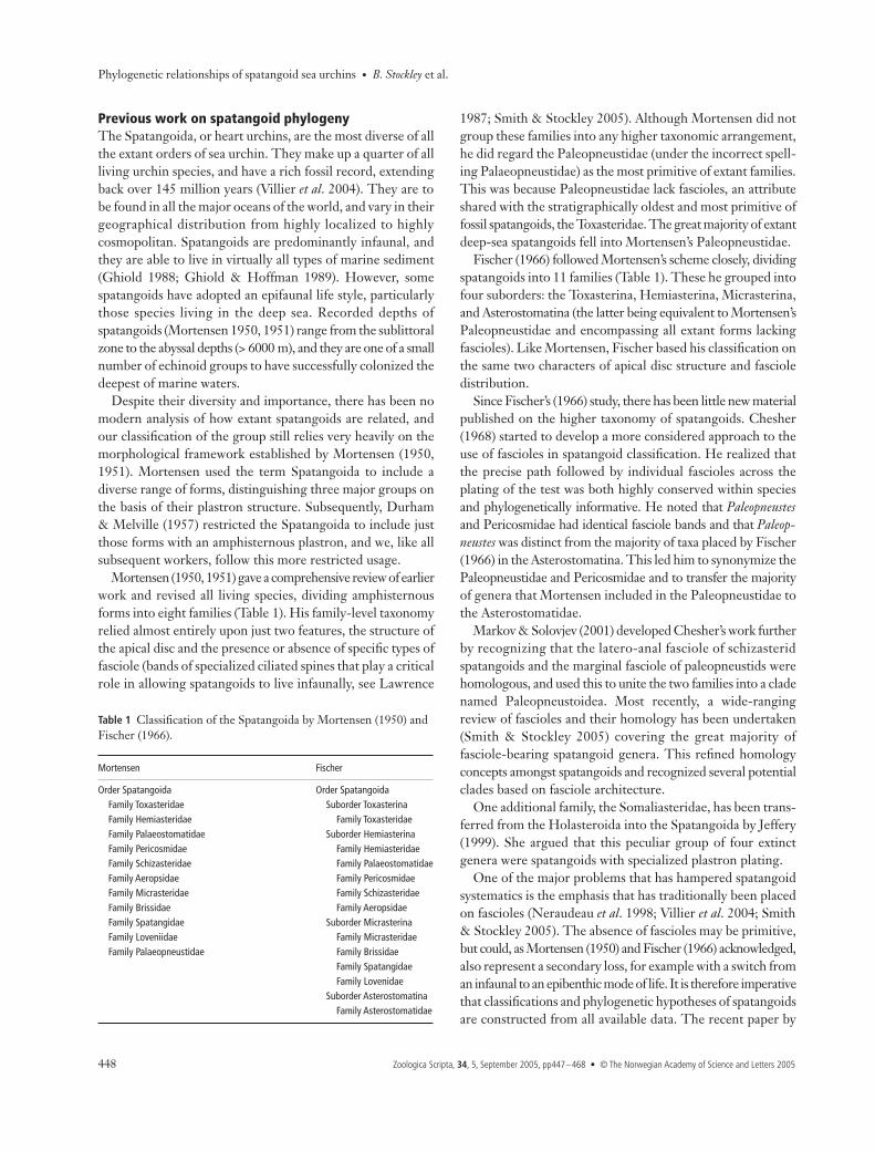
Mortensen (1950, 1951) gave a comprehensive review of earlierwork and revised all living species, dividing amphisternousforms into eight families (Table 1). His family-level taxonomyrelied almost entirely upon just two features, the structure ofthe apical disc and the presence or absence of specific types offasciole (bands of specialized ciliated spines that play a criticalrole in allowing spatangoids to live infaunally, see Lawrence
1987; Smith & Stockley 2005). Although Mortensen did notgroup these families into any higher taxonomic arrangement,he did regard the Paleopneustidae (under the incorrect spell-ing Palaeopneustidae) as the most primitive of extant families.This was because Paleopneustidae lack fascioles, an attributeshared with the stratigraphically oldest and most primitive offossil spatangoids, the Toxasteridae. The great majority of extantdeep-sea spatangoids fell into Mortensen’s Paleopneustidae.
Fischer (1966) followed Mortensen’s scheme closely, dividingspatangoids into 11 families (Table 1). These he grouped intofour suborders: the Toxasterina, Hemiasterina, Micrasterina,and Asterostomatina (the latter being equivalent to Mortensen’sPaleopneustidae and encompassing all extant forms lackingfascioles). Like Mortensen, Fischer based his classification onthe same two characters of apical disc structure and fascioledistribution.
Since Fischer’s (1966) study, there has been little new materialpublished on the higher taxonomy of spatangoids. Chesher(1968) started to develop a more considered approach to theuse of fascioles in spatangoid classification. He realized thatthe precise path followed by individual fascioles across theplating of the test was both highly conserved within speciesand phylogenetically informative. He noted that
Paleopneustes
and Pericosmidae had identical fasciole bands and that
Paleop-neustes
was distinct from the majority of taxa placed by Fischer(1966) in the Asterostomatina. This led him to synonymize thePaleopneustidae and Pericosmidae and to transfer the majorityof genera that Mortensen included in the Paleopneustidae tothe Asterostomatidae.
Markov & Solovjev (2001) developed Chesher’s work furtherby recognizing that the latero-anal fasciole of schizasteridspatangoids and the marginal fasciole of paleopneustids werehomologous, and used this to unite the two families into a cladenamed Paleopneustoidea. Most recently, a wide-rangingreview of fascioles and their homology has been undertaken(Smith & Stockley 2005) covering the great majority offasciole-bearing spatangoid genera. This refined homologyconcepts amongst spatangoids and recognized several potentialclades based on fasciole architecture.
One additional family, the Somaliasteridae, has been trans-ferred from the Holasteroida into the Spatangoida by Jeffery(1999). She argued that this peculiar group of four extinctgenera were spatangoids with specialized plastron plating.
One of the major problems that has hampered spatangoidsystematics is the emphasis that has traditionally been placedon fascioles (Neraudeau
et al
. 1998; Villier
et al
. 2004; Smith& Stockley 2005). The absence of fascioles may be primitive,but could, as Mortensen (1950) and Fischer (1966) acknowledged,also represent a secondary loss, for example with a switch froman infaunal to an epibenthic mode of life. It is therefore imperativethat classifications and phylogenetic hypotheses of spatangoidsare constructed from all available data. The recent paper by
Table 1 Classification of the Spatangoida by Mortensen (1950) and Fischer (1966).
Mortensen Fischer
Order Spatangoida Order SpatangoidaFamily Toxasteridae Suborder ToxasterinaFamily Hemiasteridae Family ToxasteridaeFamily Palaeostomatidae Suborder HemiasterinaFamily Pericosmidae Family HemiasteridaeFamily Schizasteridae Family PalaeostomatidaeFamily Aeropsidae Family PericosmidaeFamily Micrasteridae Family SchizasteridaeFamily Brissidae Family AeropsidaeFamily Spatangidae Suborder MicrasterinaFamily Loveniidae Family MicrasteridaeFamily Palaeopneustidae Family Brissidae
Family SpatangidaeFamily Lovenidae
Suborder AsterostomatinaFamily Asterostomatidae
B. Stockley
et al.
•
Phylogenetic relationships of spatangoid sea urchins
© The Norwegian Academy of Science and Letters 2005 • Zoologica Scripta,
34
, 5, September 2005, pp447–468
449
Villier
et al
. (2004) has started this process by compiling a largedatabase of morphological characters for the early Creta-ceous genera of Spatangoida and subjecting it to a rigorouscladistic analysis. Their study examined a broad cross-sectionof primitive taxa and found support for Fischer’s Micrasterinaand Hemiasterina groupings; however, they did not includetaxa younger than mid-Cretaceous.
In this paper we provide a dual molecular and morphologicalanalysis of spatangoid phylogeny to generate a phylogeny andrevised taxonomy for the entire group, investigate how manyindependent lineages are living in the deep sea, and explorethe value of wider taxon sampling.
Materials and methods
Taxa and outgroups
Twenty-one species of Spatangoida, representing 18 genera,and five of Mortensen’s eight extant families (Table 2), form thecore of this study. Three genera —
Brisaster
(Schizasteridae),
Metalia
(Brissidae), and
Spatangus
(Spatangidae) — were eachrepresented by two species so that regions of highly variablegene sequence at the congeneric level could be identifiedand removed. Morphological data were collected for these21 species as well as for a much larger sample of taxa comprising88 genera, both Recent and fossil. In almost all cases type specieswere selected as exemplars for the genera. Information on thesetaxa is available in Smith (2004).
As outgroup for the morphological analyses we used
Toxasterretusus
, one of the stratigraphically earliest fossils and one that
has traditionally been considered as one of the most primitive(Mortensen 1950, 1951; Fischer 1966; Villier
et al
. 2004). Forrooting molecular data we used three outgroups:
Plexechinus
,
Echinoneus
and
Conolampas
.
Plexechinus
is a member of theHolasteroida, the closest extant sister group to spatangoids,and split from Spatangoida approximately 140 million yearsago.
Conolampas
is a representative of the Cassiduloida anddiverged from spatangoids about 180 million years ago, while
Echinoneus
is considered to be the most primitive livingirregular echinoid (Smith & Wright 1999).
Morphological methods
All morphological characters used in this study were definedby direct examination of specimens, using a low powerlight microscope. Seventy-nine characters relating to skeletalarchitecture and tuberculation were scored. The full list ofcharacters, with descriptions of character states and coding,is given in Appendix 1. Data on pedicellarial morphologywere also collected but quickly abandoned as they provedto be highly variable amongst extant species and unavailablefrom fossil taxa.
All but three of the characters (6, 46, 77) were treated asunordered. Three characters, relating to the development ofthe frontal groove (depth of groove adapically, at ambitus andadorally; characters 8–10 in Appendix 1) were each given aweight of 0.333 so as to give the character ‘development offrontal groove’ the same weight as other test features. All othercharacters were given equal weight.
Genus Species Author 28S 16S COI
Abatus cavernosus Philippi (1845) AJ639776 AJ639803 AJ639904Agassizia scrobiculata Valenciennes (1846) AJ639779 AJ639802Allobrissus agassizii Doderlein (1885) AJ639799 AJ639823 AJ639920Amphipneustes lorioli Koehler (1901) AJ639780 AJ639804 AJ639905Archaeopneustes hystrix A. Agassiz (1880) AJ639785 AJ639809 AJ639909Brisaster fragilis Duben & Koren (1844) AJ639781 AJ639805 AJ639906Brisaster latifrons A. Agassiz (1898) AJ639782 AJ639806Brissopsis atlantica Mortensen (1907) AJ639794 AJ639818 AJ639917Brissus obessus Verrill (1867) AJ639797 AJ639821Conolampas sigsbei A. Agassiz (1878) AJ639777 AJ639800 AJ639902Echinocardium laevigaster A. Agassiz (1869) AJ639789 AJ639813 AJ639913Echinoneus cyclostomus Leske (1778) AJ639778 AJ639801 AJ639903Linopneustes longispinus A. Agassiz (1878) AJ639795 AJ639819 AJ639918Lovenia cordiformis A. Agassiz (1872) AJ639790 AJ639814 AJ639914Meoma ventricosa Lamarck (1816) AJ639796 AJ639820 AJ639919Metalia spatagus Linnaeus (1758) AJ639791 AJ639815 AJ639915Metalia nobilis Verrill (1867–71) AJ639792 AJ639816Paleopneustes cristatus A. Agassiz (1873) AJ639784 AJ639808 AJ639908Paramaretia multituberculata Mortensen (1950) AJ639788 AJ639812 AJ639912Paraster doederleni Chesher (1972) AJ639783 AJ639807 AJ639907Plagiobrissus grandis Gmelin (1788) AJ639793 AJ639817 AJ639916Plexechinus planus Mironov (1978) AY957469 AY957467Spatangus raschi Loven (1869) AJ639787 AJ639811 AJ639911Spatangus multispinus Mortensen (1925) AJ639786 AJ639810 AJ639910
Table 2 Spatangoid taxa sequenced with EMBL/GenBank database accession numbers given where sequence data was produced.
Phylogenetic relationships of spatangoid sea urchins
•
B. Stockley
et al.
450
Zoologica Scripta,
34
, 5, September 2005, pp447–468 • © The Norwegian Academy of Science and Letters 2005
Phylogenetic analysis was carried out using the Macintoshversion of
PAUP
* 4.0b10 (Altivec) (Swofford 2002). As the largenumber of taxa precluded a branch and bound or exhaustivesearch of the matrix, we used a heuristic search method, withrandom additional replicates and TBR branch swapping. Boot-strapping was carried out to test node support and Bremersupport was also calculated (Bremer 1994).
Two analyses were run: one using the full set of 88 taxa (fulldataset) and the other including just those genera for whichmolecular data were available, plus an outgroup (19 genera —the core dataset). For the core dataset, 2000 random additionreplicates were run and bootstrapping was carried out with1000 replicates. Heuristic searches of the full dataset of88 taxa proved to be much more time-consuming and just25 random replicates were run. This generated multiple equallyparsimonious trees and so the characters were then reweightedby the maximum rescaled consistency index of the initial trees(weightings used are given in Table 3) and the analysis rerunwith 1000 random addition replicates.
Molecular methods
Gene selection.
Three genes were selected for analysis: themitochondrial 16S rRNA (16S), cytochrome c oxidase subunit1 (COI) and nuclear 28S rRNA (28S) genes. These were chosenbecause they had been used successfully in earlier studies(Littlewood & Smith 1995; Jeffery
et al
. 2003) and were knownto encompass the range of rates of evolution needed to resolvedivergences over the past 150 million years. Approximately630 base pairs from the 3
′
end of the 16S gene, 800 base pairsfrom the 5
′
end of the COI gene and 1250 base pairs from the5
′
end of the 28S gene were amplified.
DNA extraction, amplification, sequencing and alignment
Specimens were freshly collected and either frozen or fixed inabsolute ethanol prior to tissue extraction. Several microgramsof tissue were excised from specimens. Gonadal material wasused preferentially, but, where unavailable, tissue was obtainedfrom phyllode tube feet, primary spine muscle, or peristomialmembrane. Tissue from ethanol-preserved specimens was washedin distilled water prior to DNA extraction, whilst tissue fromfrozen specimens was simply defrosted. Whole genomic DNAwas extracted using a DNeasy tissue kit (Qiagen), according
to the manufacturer’s protocol. In cases where subsequent PCRamplification failed, this whole genomic DNA was furtherpurified by using a QIAquick PCR purification column(Qiagen) according to the manufacturer’s protocol.
Amplifications of 16S and 28S fragments were performedusing the HotStarTaq PCR amplification kit (Qiagen), with20
µ
L reaction volumes. Each reaction tube contained 1–5
µ
L(approx 20 ng) of genomic DNA extract, 1 U Taq polymerase,2.5 m
M
MgCl
2
, 1X PCR buffer (proprietary, Qiagen), 1X ‘Q’solution (proprietary, Qiagen), and 10 picomoles of each externalPCR primer (Table 4). PCR conditions used were: 15-minutedenaturation at 95
°
C; 35 cycles of 50 s at 94
°
C, 50 s at52
°
C, 60 s at 72
°
C, then held at 4
°
C until used.Amplifications of COI fragments were performed using the
BioTaq DNA polymerase kit (Bioline), with 20
µ
L reactionvolumes. Each reaction tube contained; 5
µ
L (approx 40 ng) ofgenomic DNA extract, 2.5 U Taq polymerase, 2.5 m
M
MgCl
2
(1X PCR buffer (containing 8 m
M
(NH
4
)
2
SO
4
, 33.5 m
M
Tris-HCl (pH 8.8 at 25
°
C), 0.005% Tween-20), 1X ‘BioEnhance’solution (Proprietary, BioLine), and 10 picomoles of each externalPCR primer (Table 4). PCR conditions used were 4-minutedenaturation at 94
°
C, 35 cycles of 50 s at 94
°
C, 30 s at52
°
C, 60 s at 72
°
C, then held at 72
°
C for 5 min, then heldat 4
°
C until used.PCR products were purified with Qiagen Qiaquick columns,
and cycle-sequenced directly using ABI Big-Dye chemistry,according to manufacturers’ protocols. The sequencing reac-tions were purified using ethanol precipitation, and run on anABI Prism 377 autosequencer. 16S fragments were sequencedusing only internal primers, but the 28S fragments weresequenced in several overlapping subsections using a varietyof internal primers listed in Table 4.
Sequence data were obtained for both forward and reversereads of each fragment, to check base-pair reads. An initial pairwisealignment was made using MacClade (Maddison & Maddison2001) followed by alignment of sequences by eye. Areas of highvariability, and with strong within-genus variability in particularfor which no reliable alignment could be made, were excludedfrom further data analysis. Two short regions in the 16S rRNAgene could be aligned unambiguously for just the spatangoid taxabut not with outgroups included. Rather than omitting theseregions and thereby throwing away potentially phylogenetically
Table 3 Character weighting scheme (a posteriori, based on maximum rescaled consistency index).
1 (0.071429), 2 (0.134615), 3 (0.277778), 4 (0.088319), 5 (1.00000), 6 (0.622222), 7 (0.222222), 8 (0.055000), 9 (0.031008), 10 (0.057143), 11 (0.104072), 12 (0.134615), 13 (0.125000), 14 (0.000000), 15 (0.074074), 16 (0.080808), 17 (0.060185), 18 (1.000000), 19 (1.000000), 20 (0.064327), 21 (0.123932), 22 (1.000000), 23 (0.123377), 24 (0.107143), 25 (1.000000), 26 (0.000000), 27 (0.178571), 28 (0.047059), 29 (0.250000), 30 (0.078189), 31 (0.166667), 32 (0.107143), 33 (0.071111), 34 (0.119555), 35 (0.000000), 36 (0.166667), 37 (1.000000), 38 (1.000000), 39 (0.312500), 40 (1.000000), 41 (0.368421), 42 (0.315789), 43 (0.092593), 44 (0.154286), 45 (0.083810), 46 (0.103955), 47 (0.000000), 48 (0.000000), 49 (0.084615), 50 (0.333333), 51 (0.075000), 52 (1.000000), 53 (1.000000), 54 (0.485294), 55 (0.303030), 56 (1.000000), 57 (1.000000), 58 (0.105882), 59 (0.066667), 60 (1.000000), 61 (0.051383), 62 (0.070312), 63 (0.470588), 64 (1.000000), 65 (0.166667), 66 (0.146667), 67 (0.000000), 68 (0.244444), 69 (0.062500), 70 (0.054545), 71 (0.333333), 72 (1.000000), 73 (0.000000), 74 (0.0466667), 75 (0.142857), 76 (1.000000), 77 (0.266667), 78 (0.238095), 79 (0.110672)
B. Stockley
et al.
•
Phylogenetic relationships of spatangoid sea urchins
© The Norwegian Academy of Science and Letters 2005 • Zoologica Scripta,
34
, 5, September 2005, pp447–468
451
informative sites, these regions were included but with theoutgroup taxa scored as unkown (?). In total, out of 2225aligned base pairs, 465 were phylogenetically informative.
All sequences are lodged with EMBO, under acquisitionnumbers listed in Table 2.
Analysis methods used
Analysis using the optimality criterion of maximum parsimony(MP) was performed using the same version of
PAUP
* as usedin the morphological methods. Gaps were treated as missingdata (because there were so few, treating gaps as a new (5th)
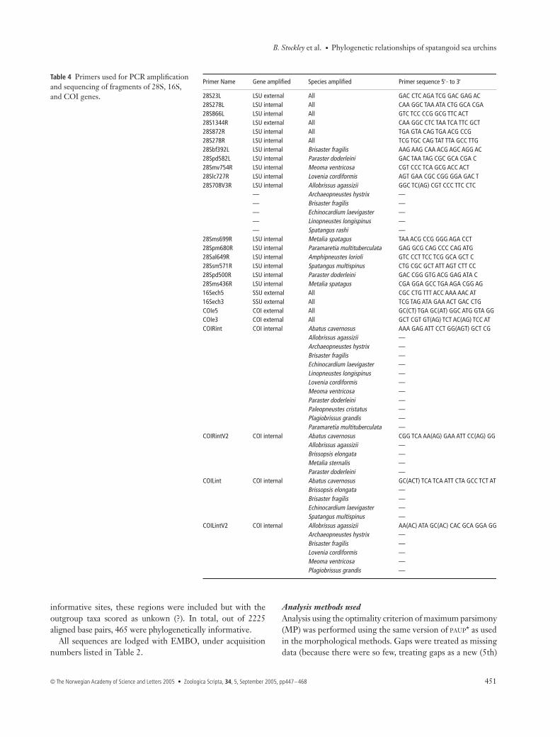
Primer Name Gene amplified Species amplified Primer sequence 5′- to 3′
28S23L LSU external All GAC CTC AGA TCG GAC GAG AC28S278L LSU internal All CAA GGC TAA ATA CTG GCA CGA28S866L LSU internal All GTC TCC CCG GCG TTC ACT28S1344R LSU external All CAA GGC CTC TAA TCA TTC GCT28S872R LSU internal All TGA GTA CAG TGA ACG CCG28S278R LSU internal All TCG TGC CAG TAT TTA GCC TTG28Sbf392L LSU internal Brisaster fragilis AAG AAG CAA ACG AGC AGG AC28Spd582L LSU internal Paraster doderleini GAC TAA TAG CGC GCA CGA C28Smv754R LSU internal Meoma ventricosa CGT CCC TCA GCG ACC ACT28Slc727R LSU internal Lovenia cordiformis AGT GAA CGC CGG GGA GAC T28S708V3R LSU internal Allobrissus agassizii GGC TC(AG) CGT CCC TTC CTC
— Archaeopneustes hystrix —— Brisaster fragilis —— Echinocardium laevigaster —— Linopneustes longispinus —— Spatangus rashi —
28Sms699R LSU internal Metalia spatagus TAA ACG CCG GGG AGA CCT28Spm680R LSU internal Paramaretia multituberculata GAG GCG CAG CCC CAG ATG28Sal649R LSU internal Amphipneustes lorioli GTC CCT TCC TCG GCA GCT C28Ssm571R LSU internal Spatangus multispinus CTG CGC GCT ATT AGT CTT CC28Spd500R LSU internal Paraster doderleini GAC CGG GTG ACG GAG ATA C28Sms436R LSU internal Metalia spatagus CGA GGA GCC TGA AGA CGG AG16Sech5 SSU external All CGC CTG TTT ACC AAA AAC AT16Sech3 SSU external All TCG TAG ATA GAA ACT GAC CTGCOIe5 COI external All GC(CT) TGA GC(AT) GGC ATG GTA GGCOIe3 COI external All GCT CGT GT(AG) TCT AC(AG) TCC ATCOIRint COI internal Abatus cavernosus AAA GAG ATT CCT GG(AGT) GCT CG
Allobrissus agassizii —Archaeopneustes hystrix —Brisaster fragilis —Echinocardium laevigaster —Linopneustes longispinus —Lovenia cordiformis —Meoma ventricosa —Paraster doderleini —Paleopneustes cristatus —Plagiobrissus grandis —Paramaretia multituberculata —
COIRintV2 COI internal Abatus cavernosus CGG TCA AA(AG) GAA ATT CC(AG) GGAllobrissus agassizii —Brissopsis elongata —Metalia sternalis —Paraster doderleini —
COILint COI internal Abatus cavernosus GC(ACT) TCA TCA ATT CTA GCC TCT ATBrissopsis elongata —Brisaster fragilis —Echinocardium laevigaster —Spatangus multispinus —
COILintV2 COI internal Allobrissus agassizii AA(AC) ATA GC(AC) CAC GCA GGA GGArchaeopneustes hystrix —Brisaster fragilis —Lovenia cordiformis —Meoma ventricosa —Plagiobrissus grandis —
Table 4 Primers used for PCR amplification and sequencing of fragments of 28S, 16S, and COI genes.
Phylogenetic relationships of spatangoid sea urchins • B. Stockley et al.
452 Zoologica Scripta, 34, 5, September 2005, pp447–468 • © The Norwegian Academy of Science and Letters 2005
state made no difference to the resultant trees). All characterstate transformations were treated as of equal weight. Datasets were bootstrapped with 1000 replicates.
Modeltest v. 3.06 for Macintosh (Posada & Crandall 1998)was used to analyse each data set and produce an appropriatemodel of genetic evolution for maximum likelihood (ML) andBayes analysis. Two different models were used: for ML weused the simpler HKY85 model with transition-transversionratio and base frequencies estimated empirically, for Bayesanalyses we used the GTR + G + I model (rates set to gamma,with six substitution types). Bayesian inference analyses wereconducted using a separate GTR + G + I model for each datapartition independently, and also for the combined three-gene analysis, thus allowing separate estimates for each modelparameter per data set.
ML analysis was performed using the same version of PAUP*as the MP analysis. The maximum number of trees in memorywas not limited. Data sets were bootstrapped with 150 replicates.
Bayes analysis was performed using both the Macintosh andthe Unix versions of MrBayes (Huelsenbeck & Ronquist 2003).The number of generations permitted was 1 000 000 with fourchains, and a burn in of 5000. The consensus tree was constructedfrom the nonburn in trees, and was a 50% majority rule tree.
Data congruence testsTo investigate the appropriateness of combining the gene datasets, the Partition Homogeneity (Farris et al. 1994) option inPAUP* was executed.
A Templeton test of data heterogeneity (described by Larson1994; and implemented in PAUP* under the ‘describe trees’
option) was performed on the various trees that were obtainedfrom morphological and molecular data sets under the differentanalytical procedures, to explore whether they could be con-sidered suboptimal estimates of the same underlying topology.For comparison, the tree generated from morphological dataand based on 88 taxa was pruned so that it contained only thosetaxa common to the molecular data sets being compared.
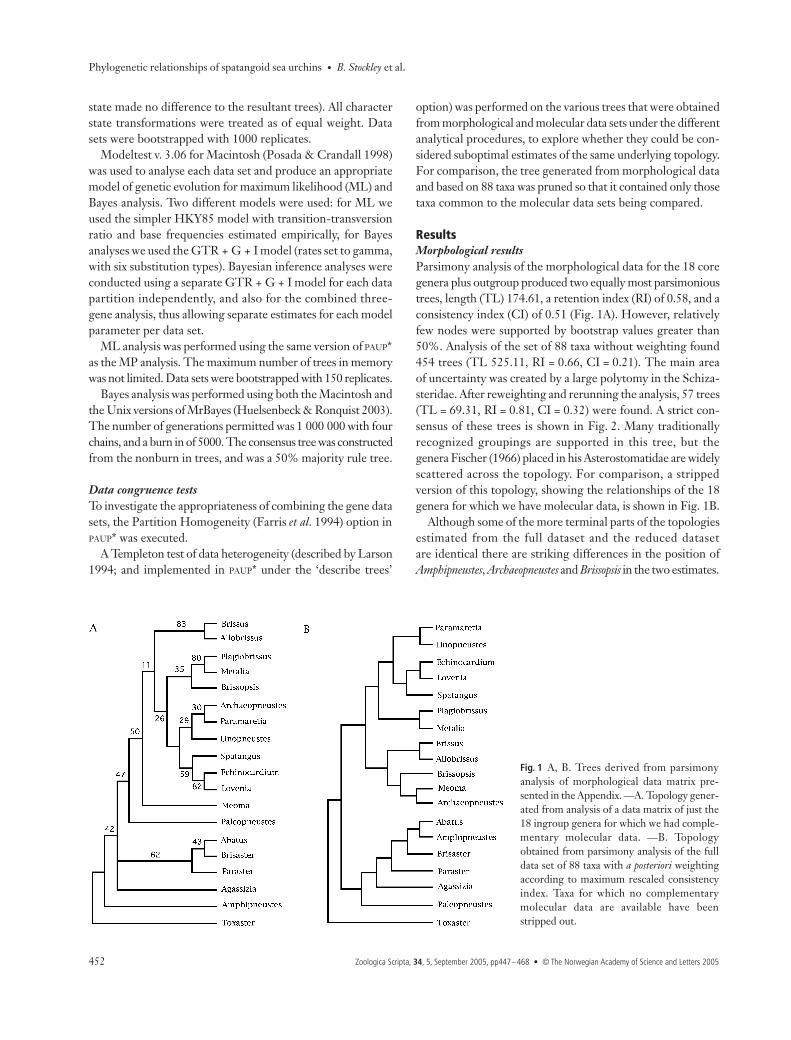
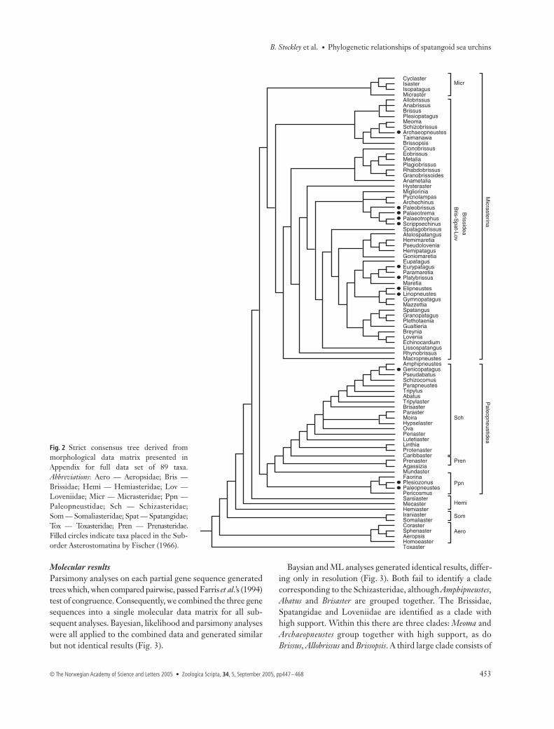
ResultsMorphological resultsParsimony analysis of the morphological data for the 18 coregenera plus outgroup produced two equally most parsimonioustrees, length (TL) 174.61, a retention index (RI) of 0.58, and aconsistency index (CI) of 0.51 (Fig. 1A). However, relativelyfew nodes were supported by bootstrap values greater than50%. Analysis of the set of 88 taxa without weighting found454 trees (TL 525.11, RI = 0.66, CI = 0.21). The main areaof uncertainty was created by a large polytomy in the Schiza-steridae. After reweighting and rerunning the analysis, 57 trees(TL = 69.31, RI = 0.81, CI = 0.32) were found. A strict con-sensus of these trees is shown in Fig. 2. Many traditionallyrecognized groupings are supported in this tree, but thegenera Fischer (1966) placed in his Asterostomatidae are widelyscattered across the topology. For comparison, a strippedversion of this topology, showing the relationships of the 18genera for which we have molecular data, is shown in Fig. 1B.
Although some of the more terminal parts of the topologiesestimated from the full dataset and the reduced datasetare identical there are striking differences in the position ofAmphipneustes, Archaeopneustes and Brissopsis in the two estimates.
Fig. 1 A, B. Trees derived from parsimonyanalysis of morphological data matrix pre-sented in the Appendix. —A. Topology gener-ated from analysis of a data matrix of just the18 ingroup genera for which we had comple-mentary molecular data. —B. Topologyobtained from parsimony analysis of the fulldata set of 88 taxa with a posteriori weightingaccording to maximum rescaled consistencyindex. Taxa for which no complementarymolecular data are available have beenstripped out.
B. Stockley et al. • Phylogenetic relationships of spatangoid sea urchins
© The Norwegian Academy of Science and Letters 2005 • Zoologica Scripta, 34, 5, September 2005, pp447–468 453
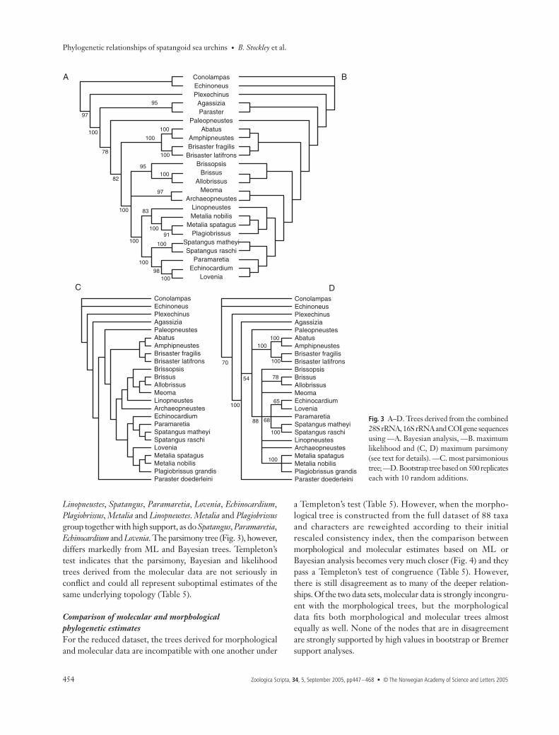
Molecular resultsParsimony analyses on each partial gene sequence generatedtrees which, when compared pairwise, passed Farris et al.’s (1994)test of congruence. Consequently, we combined the three genesequences into a single molecular data matrix for all sub-sequent analyses. Bayesian, likelihood and parsimony analyseswere all applied to the combined data and generated similarbut not identical results (Fig. 3).
Baysian and ML analyses generated identical results, differ-ing only in resolution (Fig. 3). Both fail to identify a cladecorresponding to the Schizasteridae, although Amphipneustes,Abatus and Brisaster are grouped together. The Brissidae,Spatangidae and Loveniidae are identified as a clade withhigh support. Within this there are three clades: Meoma andArchaeopneustes group together with high support, as doBrissus, Allobrissus and Brissopsis. A third large clade consists of
Fig. 2 Strict consensus tree derived frommorphological data matrix presented inAppendix for full data set of 89 taxa.Abbreviations: Aero — Aeropsidae; Bris —Brissidae; Hemi — Hemiasteridae; Lov —Loveniidae; Micr — Micrasteridae; Ppn —Paleopneustidae; Sch — Schizasteridae;Som — Somaliasteridae; Spat — Spatangidae;Tox — Toxasteridae; Pren — Prenasteridae.Filled circles indicate taxa placed in the Sub-order Asterostomatina by Fischer (1966).
Phylogenetic relationships of spatangoid sea urchins • B. Stockley et al.
454 Zoologica Scripta, 34, 5, September 2005, pp447–468 • © The Norwegian Academy of Science and Letters 2005
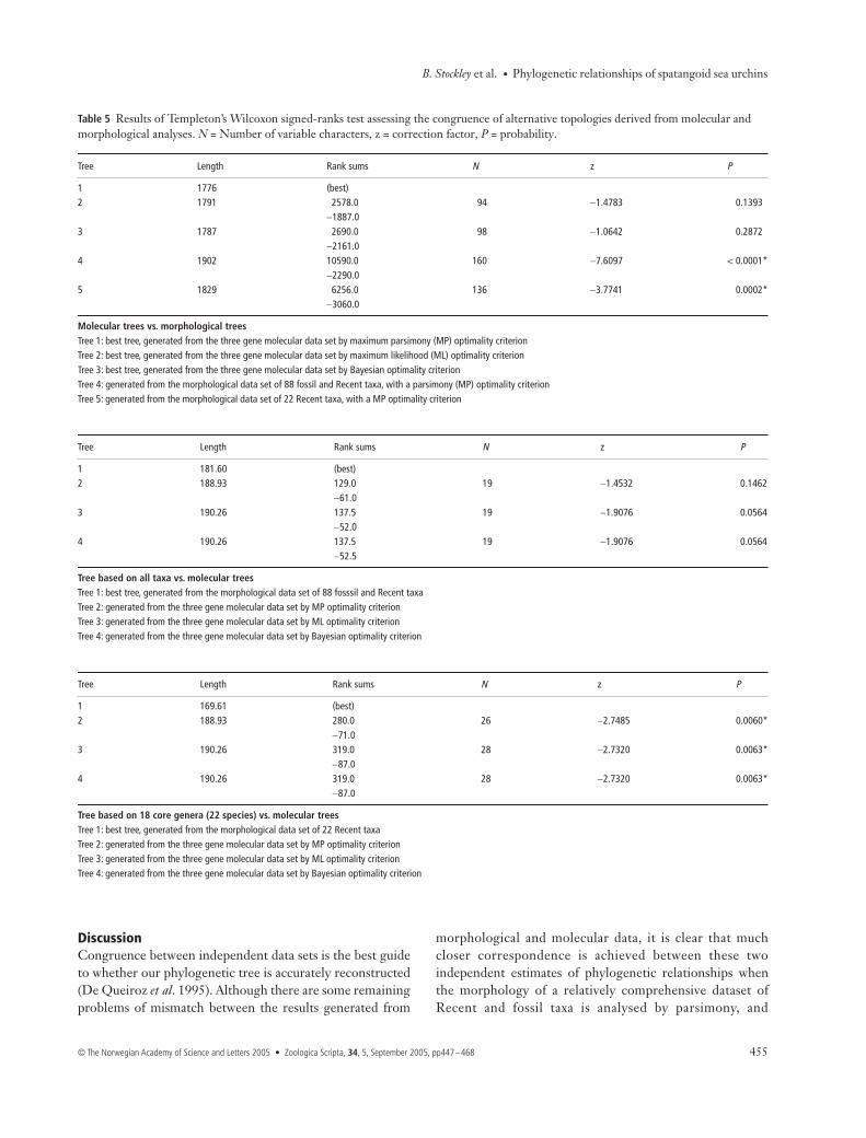
Linopneustes, Spatangus, Paramaretia, Lovenia, Echinocardium,Plagiobrissus, Metalia and Linopneustes. Metalia and Plagiobrissusgroup together with high support, as do Spatangus, Paramaretia,Echinocardium and Lovenia. The parsimony tree (Fig. 3), however,differs markedly from ML and Bayesian trees. Templeton’stest indicates that the parsimony, Bayesian and likelihoodtrees derived from the molecular data are not seriously inconflict and could all represent suboptimal estimates of thesame underlying topology (Table 5).
Comparison of molecular and morphological phylogenetic estimatesFor the reduced dataset, the trees derived for morphologicaland molecular data are incompatible with one another under
a Templeton’s test (Table 5). However, when the morpho-logical tree is constructed from the full dataset of 88 taxaand characters are reweighted according to their initialrescaled consistency index, then the comparison betweenmorphological and molecular estimates based on ML orBayesian analysis becomes very much closer (Fig. 4) and theypass a Templeton’s test of congruence (Table 5). However,there is still disagreement as to many of the deeper relation-ships. Of the two data sets, molecular data is strongly incongru-ent with the morphological trees, but the morphologicaldata fits both morphological and molecular trees almostequally as well. None of the nodes that are in disagreementare strongly supported by high values in bootstrap or Bremersupport analyses.
Fig. 3 A–D. Trees derived from the combined28S rRNA, 16S rRNA and COI gene sequencesusing —A. Bayesian analysis, —B. maximumlikelihood and (C, D) maximum parsimony(see text for details). —C. most parsimonioustree; —D. Bootstrap tree based on 500 replicateseach with 10 random additions.
B. Stockley et al. • Phylogenetic relationships of spatangoid sea urchins
© The Norwegian Academy of Science and Letters 2005 • Zoologica Scripta, 34, 5, September 2005, pp447–468 455
DiscussionCongruence between independent data sets is the best guideto whether our phylogenetic tree is accurately reconstructed(De Queiroz et al. 1995). Although there are some remainingproblems of mismatch between the results generated from
morphological and molecular data, it is clear that muchcloser correspondence is achieved between these twoindependent estimates of phylogenetic relationships whenthe morphology of a relatively comprehensive dataset ofRecent and fossil taxa is analysed by parsimony, and
Table 5 Results of Templeton’s Wilcoxon signed-ranks test assessing the congruence of alternative topologies derived from molecular and morphological analyses. N = Number of variable characters, z = correction factor, P = probability.
Tree Length Rank sums N z P
1 1776 (best)2 1791 2578.0 94 −1.4783 0.1393
−1887.03 1787 2690.0 98 −1.0642 0.2872
−2161.04 1902 10590.0 160 −7.6097 < 0.0001*
−2290.05 1829 6256.0 136 −3.7741 0.0002*
−3060.0
Molecular trees vs. morphological treesTree 1: best tree, generated from the three gene molecular data set by maximum parsimony (MP) optimality criterion Tree 2: best tree, generated from the three gene molecular data set by maximum likelihood (ML) optimality criterion Tree 3: best tree, generated from the three gene molecular data set by Bayesian optimality criterion Tree 4: generated from the morphological data set of 88 fossil and Recent taxa, with a parsimony (MP) optimality criterion Tree 5: generated from the morphological data set of 22 Recent taxa, with a MP optimality criterion
Tree Length Rank sums N z P
1 181.60 (best)2 188.93 129.0 19 −1.4532 0.1462
−61.03 190.26 137.5 19 −1.9076 0.0564
−52.04 190.26 137.5 19 −1.9076 0.0564
−52.5
Tree based on all taxa vs. molecular trees Tree 1: best tree, generated from the morphological data set of 88 fosssil and Recent taxa Tree 2: generated from the three gene molecular data set by MP optimality criterion Tree 3: generated from the three gene molecular data set by ML optimality criterion Tree 4: generated from the three gene molecular data set by Bayesian optimality criterion
Tree Length Rank sums N z P
1 169.61 (best)2 188.93 280.0 26 −2.7485 0.0060*
−71.03 190.26 319.0 28 −2.7320 0.0063*
−87.04 190.26 319.0 28 −2.7320 0.0063*
−87.0
Tree based on 18 core genera (22 species) vs. molecular trees Tree 1: best tree, generated from the morphological data set of 22 Recent taxa Tree 2: generated from the three gene molecular data set by MP optimality criterion Tree 3: generated from the three gene molecular data set by ML optimality criterion Tree 4: generated from the three gene molecular data set by Bayesian optimality criterion
Phylogenetic relationships of spatangoid sea urchins • B. Stockley et al.
456 Zoologica Scripta, 34, 5, September 2005, pp447–468 • © The Norwegian Academy of Science and Letters 2005
homoplasy of characters is taken into account by a posteriorireweighting.
The results are not identical, but are sufficiently closethat the two estimates pass a Templeton’s test of congruence inboth directions. By contrast, when our phylogenetic analysisof morphological data was restricted to just the small numberof taxa for which molecular data are available, results wereincongruent, and the two independent estimates of phylo-genetic relationships appeared to be in conflict. Therefore, inthis case, we believe that model-based analyses of moleculardata and parsimony-based analyses of morphological charactersdensely sampled across taxa with a posteriori weighting provideour most accurate phylogenetic hypothesis of spatangoidrelationships.
What then might be causing the differences betweenour molecular and morphological estimates? First, the resultsgenerated from the molecular data are to some degreesensitive to the analytical technique used and the initialassumptions made. Parsimony, likelihood and Bayes analysesincorporated successively more specific models of evolutionand did not produce the same topology (Fig. 3). However, thetwo methods that weighed transversions as less likely thantransitions generated congruent trees.
Sampling density, in the form of either taxon samplingor gene sampling, probably lies at the root of the differenceswe have observed between our morphological and molecularanalyses. Previous studies (e.g. Hillis 1996, 1998; Givnish &Sytsma 1997) have focused on the role of character samplingand have emphasized that greater accuracy is achieved as morecharacters are added to an analysis. Although this certainly appliesto molecular data, it is less obvious that this is also the casefor morphological data (Lamboy 1994; Wiens & Hillis 1996;Scotland et al. 2003). Here, taxon sampling may have a morepotent effect on a tree. Rosenberg & Kumar (2001) argued thatfor molecular datasets incomplete taxonomic sampling wasunlikely to generate misleading results as long as sufficientlylarge numbers of variable characters were available. By contrast,morphologists have argued that denser sampling of taxa,especially fossil taxa, is of great importance for tree accuracy(Gauthier et al. 1988; Smith 1998; Wills et al. 1998; Poe 1998).
The importance of dense taxon sampling is evident fromour morphological data. The results that we obtained fromparsimony analysis of the reduced dataset are significantlydifferent from both the molecular estimates and the estimatebased on a much denser sampling of taxa. In this case, sparsesampling is exacerbated by another factor: many of the deep-seagroups appear to have undergone secondary morphologicalsimplification involving the loss of fascioles and reduction orcomplete loss of petals.
Fascioles are essential structures for an infaunal mode oflife, providing both a pump for ciliary driven water currentswithin the burrow and a mucous sheath for binding the burrowwalls (Lawrence 1987). However, they serve no purpose inepibenthic species and are therefore commonly lost in deep-sea forms. Similarly, the highly developed respiratory zonesof tube feet that form the petals are essential for shallowwater spatangoids, but are commonly simplified or absentin deep-sea representatives where respiratory needs are lessdemanding and the body wall much thinner. With limitedtaxon sampling, the absence of petals and fascioles is interpretedas plesiomorphic and such taxa are pulled to a basal position.When denser sampling, that includes the immediate fasciole-bearing and petaloid sister groups to the deeper watertaxa (many of which are fossil), is available, such absencesare recognized as being secondary reversals and a differenttopology results.
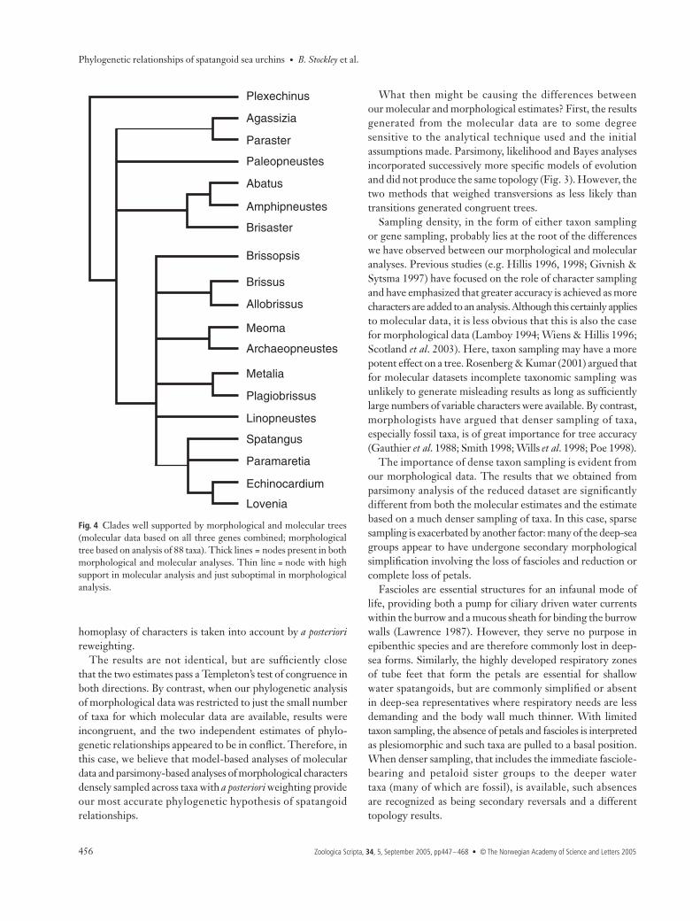
Fig. 4 Clades well supported by morphological and molecular trees(molecular data based on all three genes combined; morphologicaltree based on analysis of 88 taxa). Thick lines = nodes present in bothmorphological and molecular analyses. Thin line = node with highsupport in molecular analysis and just suboptimal in morphologicalanalysis.
B. Stockley et al. • Phylogenetic relationships of spatangoid sea urchins
© The Norwegian Academy of Science and Letters 2005 • Zoologica Scripta, 34, 5, September 2005, pp447–468 457
A key point worth emphasizing is that adding more taxareduces the character to taxon ratio for morphological traitsbut may improve the accuracy of the tree topology. Therefore,the number of taxa sampled could be of greater importanceto tree accuracy than the number of characters per taxon,contrary to the assertion of Scotland et al. (2003).
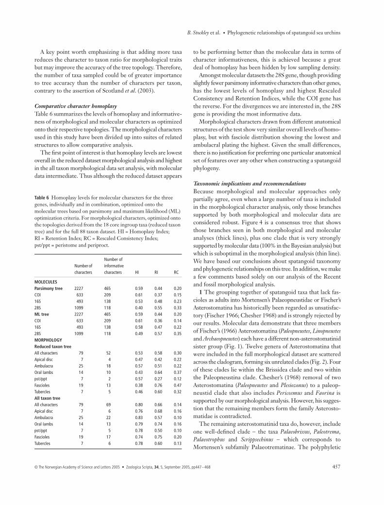
Comparative character homoplasyTable 6 summarizes the levels of homoplasy and informative-ness of morphological and molecular characters as optimizedonto their respective topologies. The morphological charactersused in this study have been divided up into suites of relatedstructures to allow comparative analysis.
The first point of interest is that homoplasy levels are lowestoverall in the reduced dataset morphological analysis and highestin the all taxon morphological data set analysis, with moleculardata intermediate. Thus although the reduced dataset appears
to be performing better than the molecular data in terms ofcharacter informativeness, this is achieved because a greatdeal of homoplasy has been hidden by low sampling density.
Amongst molecular datasets the 28S gene, though providingslightly fewer parsimony informative characters than other genes,has the lowest levels of homoplasy and highest RescaledConsistency and Retention Indices, while the COI gene hasthe reverse. For the divergences we are interested in, the 28Sgene is providing the most informative data.
Morphological characters drawn from different anatomicalstructures of the test show very similar overall levels of homo-plasy, but with fasciole distribution showing the lowest andambulacral plating the highest. Given the small differences,there is no justification for preferring one particular anatomicalset of features over any other when constructing a spatangoidphylogeny.
Taxonomic implications and recommendationsBecause morphological and molecular approaches onlypartially agree, even when a large number of taxa is includedin the morphological character analysis, only those branchessupported by both morphological and molecular data areconsidered robust. Figure 4 is a consensus tree that showsthose branches seen in both morphological and molecularanalyses (thick lines), plus one clade that is very stronglysupported by molecular data (100% in the Bayesian analysis) butwhich is suboptimal in the morphological analysis (thin line).We have based our conclusions about spatangoid taxonomyand phylogenetic relationships on this tree. In addition, we makea few comments based solely on our analysis of the Recentand fossil morphological analysis.
1 The grouping together of spatangoid taxa that lack fas-cioles as adults into Mortensen’s Palaeopneustidae or Fischer’sAsterostomatina has historically been regarded as unsatisfac-tory (Fischer 1966; Chesher 1968) and is strongly rejected byour results. Molecular data demonstrate that three membersof Fischer’s (1966) Asterostomatina (Paleopneustes, Linopneustesand Archaeopneustes) each have a different non-asterostomatinidsister group (Fig. 1). Twelve genera of Asterostomatina thatwere included in the full morphological dataset are scatteredacross the cladogram, forming six unrelated clades (Fig. 2). Fourof these clades lie within the Brissidea clade and two withinthe Paleopneustina clade. Chesher’s (1968) removal of twoAsterostomatina (Paleopneustes and Plesiozonus) to a paleop-neustid clade that also includes Pericosmus and Faorina issupported by our morphological analysis. However, his sugges-tion that the remaining members form the family Asterosto-matidae is contradicted.
The remaining asterostomatinid taxa do, however, includeone well-defined clade − the taxa Palaeobrissus, Paleotrema,Palaeotrophus and Scrippsechinus − which corresponds toMortensen’s subfamily Palaeotrematinae. The polyphyletic
Table 6 Homoplasy levels for molecular characters for the three genes, individually and in combination, optimized onto the molecular trees based on parsimony and maximum likelihood (ML) optimization criteria. For morphological characters, optimized onto the topologies derived from the 18 core ingroup taxa (reduced taxon tree) and for the full 88 taxon dataset. HI = Homoplasy Index; RI = Retention Index; RC = Rescaled Consistency Index; pst/ppt = peristome and periproct.
Number of characters
Number of informative characters HI RI RC
MOLECULESParsimony tree 2227 465 0.59 0.44 0.20COI 633 209 0.61 0.37 0.1516S 493 138 0.53 0.48 0.2328S 1099 118 0.40 0.55 0.33ML tree 2227 465 0.59 0.44 0.20COI 633 209 0.61 0.36 0.1416S 493 138 0.58 0.47 0.2228S 1099 118 0.49 0.57 0.35MORPHOLOGYReduced taxon treeAll characters 79 52 0.53 0.58 0.30Apical disc 7 4 0.47 0.42 0.22Ambulacra 25 18 0.57 0.51 0.22Oral Iambs 14 10 0.43 0.64 0.37pst /ppt 7 2 0.57 0.27 0.12Fascioles 19 13 0.38 0.76 0.47Tubercles 7 5 0.46 0.60 0.32All taxon treeAll characters 79 69 0.80 0.66 0.14Apical disc 7 6 0.76 0.68 0.16Ambulacra 25 22 0.83 0.57 0.10Oral Iambs 14 13 0.79 0.74 0.16pst /ppt 7 5 0.78 0.50 0.10Fascioles 19 17 0.74 0.75 0.20Tubercles 7 6 0.78 0.60 0.13
Phylogenetic relationships of spatangoid sea urchins • B. Stockley et al.
458 Zoologica Scripta, 34, 5, September 2005, pp447–468 • © The Norwegian Academy of Science and Letters 2005
arrangment of the fasciole-less ‘asterostomatid’ spatangoidshighlighted by both molecular and morphological analysesstrongly implies that there were multiple origins for these deep-sea spatangoids.2 The Toxasteridae are confirmed as a basal grade, as wasalso clearly demonstrated by the work of Villier et al. (2004).The more detailed and denser sampling of toxasterids inthat paper provides the best phylogenetic hypothesis for howthese primitive taxa are related. However, we found no supportfor their grouping of Hemiasteridae and Schizasteridae intoa monophyletic Hemiasterina. By contrast, the taxa currentlyplaced in Hemiasteridae form a paraphyletic grade in ouranalysis.3 Just two large clades make up the great majority of modernspatangoids, both of which have origins around the mid-Cretaceous. These correspond to the brissid–spatangid–loveniid clade and the paleopneustid–prenasterid–schizasteridclade. The former is here referred to as the SuperfamilyBrissidea nov., while the latter was named Paleopneustoideaby Markov & Solovjev (2001: 80).4 Fischer’s (1966) detailed placement of taxa within theBrissidea into the families Spatangidae, Brissidae andLoveniidae finds little support. Although there are core cladesthat include elements of each family, the specific taxa Fischerassigned to each lie scattered throughout the Brissidea.Morphological and molecular data strongly argue for a coreBrissidae that includes Brissus and Brissopsis, and a coreLoveniidae that includes Lovenia and Echinocardium. Thereis also a core of taxa corresponding to Mortense’s (1951)subfamily Maretiinae. Meoma, which has a rather differentfasciole pattern to other brissids (Smith & Stockley 2005) isbasal to both as well as to another clade of brissid taxa unit-ing Metalia and Plagiobrissus. However, it is evident fromboth morphological and molecular analyses that the Brissidaeas constituted by Fischer (1966) represents a basal grade. Amajor focus for future work will be to establish with greaterconfidence the relationships of the various genera of Brissidea.5 The sister group to the Brissidea is formed by the Micra-steridae, which includes two living representatives, Cyclaster andIsopatagus. Micrasterids differ from Brissidea in two importantcharacters: the detailed pathway taken by the subanal fascioleand the ambulacral plate bordering the rear of the sternal plate.6 The Paleopneustidea have traditionally been separatedinto two clades, the Paleopneustidae (Pleziozonus, Paleopneustes,Pericosmus and Faorina), and the Schizasteridae. Morphologyand some molecular analyses identify these as sister taxa,but other molecular analyses place Paleopneustes within theschizasterid taxa. Neither grouping is strongly supported.There is a more serious conflict in the relative positioning ofParaster. Morphological data support Agassizia as the mostbasal and group Amphipneustes, Abatus, Brisaster and Parastertogether, whereas molecular data consistently place Paraster
as sister taxon to Agassizia. Denser sampling of taxa for bothmorphological and molecular analysis is required to resolverelationships in this part of the tree.7 There are two small clades with living representatives thatare more basal to the Paleopneustoidea plus Micrasterina.Mortensen’s and Fischer’s Hemiasteridae is, like their familyToxasteridae, a paraphyletic grade group near the base ofthe spatangoid cladogram and includes the modern genusSarsiaster.
Mortensen’s Aeropsidae contains two extant taxa but may bediphyletic. Aeropsis itself belongs to a clade that includes thelate-Cretaceous–early Palaeogene corasterids such as Sphenasterand Coraster. The other genus that Mortensen included, Aceste,is very different in appearance and may represent a highlyderived schizasterid close to Brisaster. The Aeropsidae aremore derived than the Palaeostomatidae.
AcknowledgementsWe are indebted to the following people, who kindly pro-vided tissue samples for molecular analysis: Owen Anderson,Mike Hart, Sonoko Kinjo, Benedicte Lafay, Chuck Messing,Rich Mooi, Matt Richmond, Patrick Schembri, Jon Todd,Paul Tyler and Craig Young. We would also like to thank thefollowing for access to museum holdings and type material,Sheila Halsey (Natural History Museum, London), Dave Pawsonand Jan Thompson (Smithsonian Institution), Fred Collier(Museum of Comparative Zoology, Harvard University), AgnesRage (Museum National d’Histoire Naturelle, Paris), ClausNielsen (Zoological Museum, University of Copenhagen).We also thank Rich Mooi and an anonymous referee for theirhelpful comments.
ReferencesBremer, K. (1994). Branch support and tree stability. Cladistics, 10,
295–304.Chesher, R. H. (1968). The systematics of sympatric species in West
Indian spatangoids: a revision of the genera Brissopsis, Plethotaenia,Paleopneustes, and Saviniaster. Studies in Tropical Oceanography, 7, 1–168, pls 1–35.
Cunnigham, C. W. (1997). Can three incongruence tests predictwhen data should be combined? Molecular Biology and Evolution,14, 733–740.
De Queiroz, A., Donoghue, M. J. & Kim, J. (1995). Separate versuscombined analysis of phylogenetic evidence. Annual Reviews inEcology and Systematics, 26, 657–681.
Durham, J. W. & Melville, R. V. (1957). A classification of echinoids.Journal of Paleontology, 31, 242–272.
Farris, J. S., Källersjo, M., Kluge, A. G. & Bult, C. (1994). Testingsignificance of incongruence. Cladistics, 10, 315–319.
Fischer, A. G. (1966). Spatangoida. In R. C. Moore (Ed.) Treatise onInvertebrate Paleontology. Part U, Echinodermata 3 (pp. U543–628).Boulder, CO: University of Colorado and Geological Society ofAmerica.
Gauthier, J., Kluge, A. G. & Rowe, T. (1988). Amniote phylogenyand the importance of fossils. Cladistics, 4, 105–209.
B. Stockley et al. • Phylogenetic relationships of spatangoid sea urchins
© The Norwegian Academy of Science and Letters 2005 • Zoologica Scripta, 34, 5, September 2005, pp447–468 459
Ghiold, J. (1988). Species distributions of irregular echinoids. BiologicalOceanography, 6, 79–162.
Ghiold, J. & Hoffman, A. (1989). Biogeography of spatangoid echinoids.Neue Jahrbuch für Geologie und Paläontologie Abhandlungen, 178,59–83.
Givnish, T. J. & Sytsma, K. J. (1997). Consistency, characters and thelikelihood of correct phylogenetic inference. Molecular Phylogeneticsand Evolution, 7, 320–330.
Hillis, D. M. (1996). Inferring compelx phylogenies. Nature, 383,140–141.
Hillis, D. M. (1998). Taxonomic sampling, phylogenetic accuracy,and investigator bias. Systematic Biology, 47, 3–8.
Huelsenbeck, J. P. & Ronquist, F. (2003). MrBayes (Bayesian analysisof phylogeny), Version 3.0B4. Computer program distributed by theauthors.
Janies, D. (2001). Phylogenetic relationships of extant echinodermclasses. Canadian Journal of Zoology, 79, 1232–1250.
Jeffery, C. H. (1999). A reappraisal of the phylogenetic relationshipsof somaliasterid echinoids. Palaeontology, 42, 1027–1041.
Jeffery, C. H., Emlet, R. B. & Littlewood, D. T. J. (2003). Phylogenyand evolution of developmental mode in temnopleurid echinoids.Molecular Phylogenetics and Evolution, 28, 99–118.
Kerr, A. M. & Kim, J. H. (2001). Bi-penta-bi-decaradial symmetry:a review of evolutionary and developmental trends in Holothuroi-dea (Echinodermata). Journal of Experimental Zoology (Molecular,Developmental, Evolutionary), 285, 93–103.
Lafay, B., Smith, A. B. & Christen, R. (1995). A combined morpho-logical and molecular approach to the phylogeny of asteroids(Asteroidea: Echinodermata). Systematic Biology, 44, 190–208.
Lamboy, W. F. (1994). The accuracy of maximum parsimonymethod for phylogenetic reconstruction with morphologicalcharacters. Systematic Botany, 19, 489–505.
Larson, A. (1994). The comparison of morphological and moleculardata in phylogenetic systematics. In B. Schierwater, B. Streit, G.P. Wagner & R. De Salle (Eds) Molecular Ecology and Evolution:Approaches and Applications (pp. 371–390). Basel: Birkhäuser-Verlag.
Lawrence, J. M. (1987). A Functional Biology of Echinoderms. London& Sydney: Croom-Helm.
Littlewood, D. T. J. & Smith, A. B. (1995). A combined morpholog-ical and molecular phylogeny for echinoids. Philosophical Trans-actions of the Royal Society, London B, 347, 213–234.
Littlewood, D. T. J., Smith, A. B., Clough, K. A. & Ensom, R. H.(1997). The interrelationships of the echinoderm classes: morpho-logical and molecular evidence. Biological Journal of the LinneanSociety, 61, 409–438.
Maddison, D. R. & Maddison, W. P. (2001). Macclade 4. Analysis ofPhylogeny and Character Evolution, Version 4.03. Sunderland, MA:Sinauer Associates.
Markov, A. V. & Solovjev, A. N. (2001). Echinoids of the familyPaleopneustidae (Echinoidea, Spatangoida): morphology, taxon-omy, phylogeny. Geos, 2001, 1–109.
Mortensen, T. (1950). A monograph of the Echinoidea. V. 1 Spatango-ida. I. Copenhagen: C. A. Reitzel.
Mortensen, T. (1951). A monograph of the Echinoidea. V. 1 Spatango-ida. II. Copenhagen: C. A. Reitzel.
Neraudeau, D., David, B. & Madon, C. (1998). Tuberculation inspatangoid fascioles: delineating plausible homologies. Lethaia,31, 323–334.
Poe, S. D. (1998). Sensitivity of phylogenetic estimation to taxo-nomic sampling. Systematic Biology, 47, 18–31.
Posada, D. & Crandall, K. A. (1998). MODELTEST: testing themodel of DNA substitution. Bioinformatics, 14, 817–818.
Rosenberg, M. S. & Kumar, S. (2001). Incomplete taxon sampling isnot a problem for phylogenetic inference. Proceedings of theNational Academy of Sciences USA, 908, 10751–10756.
Scotland, R. W., Olmstead, R. G. & Bennett, J. R. (2003). Phylogenyreconstruction: The role of morphology. Systematic Biology, 52,539–548.
Smith, A. B. (1998). What does palaeontology contribute to system-atics in a molecular world? Molecular Phylogenetics and Evolution, 9,437–447.
Smith, A. B. (2004). The Echinoid Directory. [electronic publication]http://www.nhm.ac.uk/palaeontology/echinoids.
Smith, A. B., Littlewood, D. T. J. & Wray, G. A. (1995a). Comparingpatterns of evolution: larval and adult life-history stages and smallribosomal RNA of post-Palaeozoic echinoids. Philosophical Trans-actions of the Royal Society, London B, 349, 11–18.
Smith, A. B., Patterson, G. L. & Lafay, B. (1995b). Ophiuroidphylogeny and higher taxonomy: morphological, molecular andpalaeontological perspectives. Zoological Journal of the LinneanSociety, 114, 213–243.
Smith, A. B., Peterson, K. J., Wray, G. & Littlewood, D. T. J. (2004).From bilateral symmetry to pentaradiality: The phylogeny of hemich-ordates and echinoderms. In J. Cracraft & M. Donoghue (Eds)The Tree of Life (pp. 365–383). Oxford: Oxford University Press.
Smith, A. B. & Stockley, B. (2005). Fasciole pathways in spatangoidechinoids: a new source of phylogenetically informative charac-ters. Zoological Journal of the Linnean Society, 144, in press.
Smith, A. B. & Wright, C. W. (1999). British Cretaceous echinoids.Part 5, Holectypoida, Echinoneoida. Monograph of the Palaeonto-graphical Society, London pp. 343–390, pls 115–129 (publicationnumber 612, part of vol. 153).
Swofford, D. L. (2002). PAUP*. Phylogenetic Analysis Using Parsimony(and Other Methods), Version 4. Sunderland, MA: Sinauer Associates.
Villier, L., Neraudeau, D., Clavel, B., Neumann, C. & David, B. (2004).Phylogeny of early Cretaceous spatangoids (Echinodermata: Echinoidea)and taxonomic implications. Palaeontology, 47, 265–292.
Wiens, J. J. & Hillis, D. M. (1996). Accuracy of parsimony analysisusing morphological data: a reappraisal. Systematic Botany, 21,237–243.
Wills, M. A., Briggs, D. E. G., Fortey, R. A., Wilkinson, M. &Sneath, P. H. A. (1998). An arthropod phylogeny based on fossiland Recent taxa. In G. D. Edgecombe (Ed.) Arthropod Fossils andPhylogeny (pp. 33–106). New York: Columbia University Press.
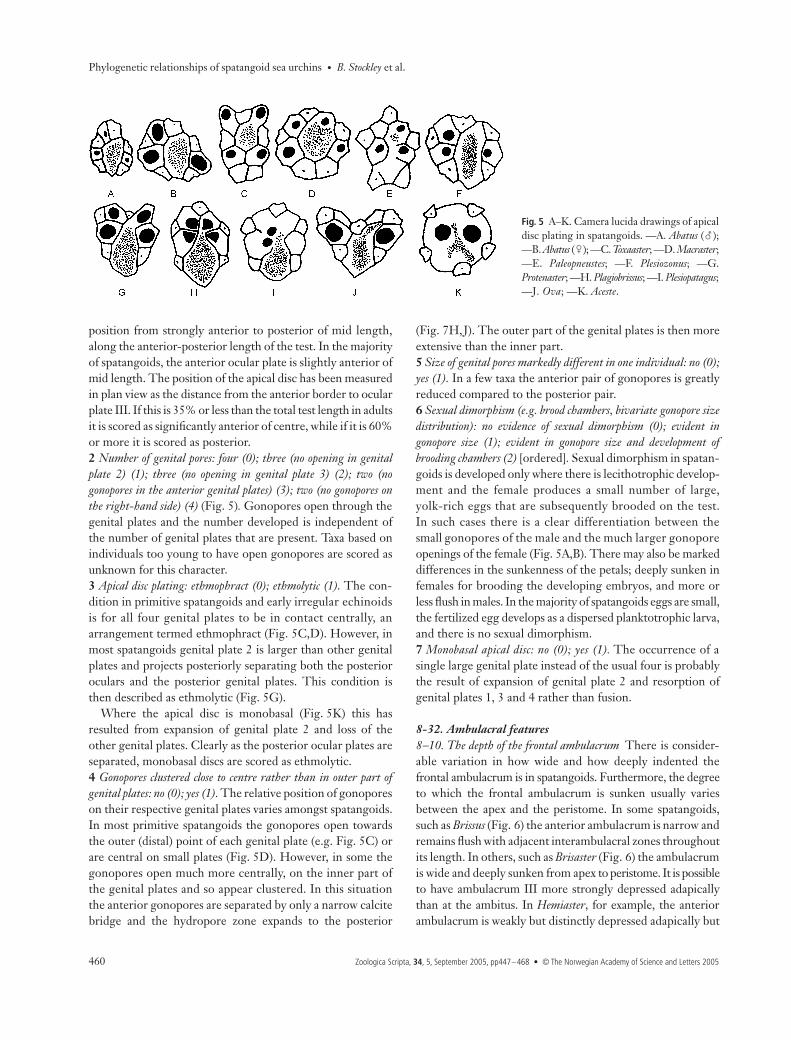
Appendix 1 Morphological characters and character state definitions used in this paper1-7. Apical discThe apical disc in spatangoids comprises five ocular platesand from one to four genital plates (Fig. 5). These form andtake on their definitive arrangement early in ontogeny and soprovide a suit of useful phylogenetic characters, as has longbeen recognized.1 Apical disc: posterior of centre (0); subcentral to slightly anterior(1); significantly anterior of centre (2). The apical disc ranges in
Phylogenetic relationships of spatangoid sea urchins • B. Stockley et al.
460 Zoologica Scripta, 34, 5, September 2005, pp447–468 • © The Norwegian Academy of Science and Letters 2005
position from strongly anterior to posterior of mid length,along the anterior-posterior length of the test. In the majorityof spatangoids, the anterior ocular plate is slightly anterior ofmid length. The position of the apical disc has been measuredin plan view as the distance from the anterior border to ocularplate III. If this is 35% or less than the total test length in adultsit is scored as significantly anterior of centre, while if it is 60%or more it is scored as posterior.2 Number of genital pores: four (0); three (no opening in genitalplate 2) (1); three (no opening in genital plate 3) (2); two (nogonopores in the anterior genital plates) (3); two (no gonopores onthe right-hand side) (4) (Fig. 5). Gonopores open through thegenital plates and the number developed is independent ofthe number of genital plates that are present. Taxa based onindividuals too young to have open gonopores are scored asunknown for this character.3 Apical disc plating: ethmophract (0); ethmolytic (1). The con-dition in primitive spatangoids and early irregular echinoidsis for all four genital plates to be in contact centrally, anarrangement termed ethmophract (Fig. 5C,D). However, inmost spatangoids genital plate 2 is larger than other genitalplates and projects posteriorly separating both the posterioroculars and the posterior genital plates. This condition isthen described as ethmolytic (Fig. 5G).
Where the apical disc is monobasal (Fig. 5K) this hasresulted from expansion of genital plate 2 and loss of theother genital plates. Clearly as the posterior ocular plates areseparated, monobasal discs are scored as ethmolytic.4 Gonopores clustered close to centre rather than in outer part ofgenital plates: no (0); yes (1). The relative position of gonoporeson their respective genital plates varies amongst spatangoids.In most primitive spatangoids the gonopores open towardsthe outer (distal) point of each genital plate (e.g. Fig. 5C) orare central on small plates (Fig. 5D). However, in some thegonopores open much more centrally, on the inner part ofthe genital plates and so appear clustered. In this situationthe anterior gonopores are separated by only a narrow calcitebridge and the hydropore zone expands to the posterior
(Fig. 7H,J). The outer part of the genital plates is then moreextensive than the inner part.5 Size of genital pores markedly different in one individual: no (0);yes (1). In a few taxa the anterior pair of gonopores is greatlyreduced compared to the posterior pair.6 Sexual dimorphism (e.g. brood chambers, bivariate gonopore sizedistribution): no evidence of sexual dimorphism (0); evident ingonopore size (1); evident in gonopore size and development ofbrooding chambers (2) [ordered]. Sexual dimorphism in spatan-goids is developed only where there is lecithotrophic develop-ment and the female produces a small number of large,yolk-rich eggs that are subsequently brooded on the test.In such cases there is a clear differentiation between thesmall gonopores of the male and the much larger gonoporeopenings of the female (Fig. 5A,B). There may also be markeddifferences in the sunkenness of the petals; deeply sunken infemales for brooding the developing embryos, and more orless flush in males. In the majority of spatangoids eggs are small,the fertilized egg develops as a dispersed planktotrophic larva,and there is no sexual dimorphism.7 Monobasal apical disc: no (0); yes (1). The occurrence of asingle large genital plate instead of the usual four is probablythe result of expansion of genital plate 2 and resorption ofgenital plates 1, 3 and 4 rather than fusion.
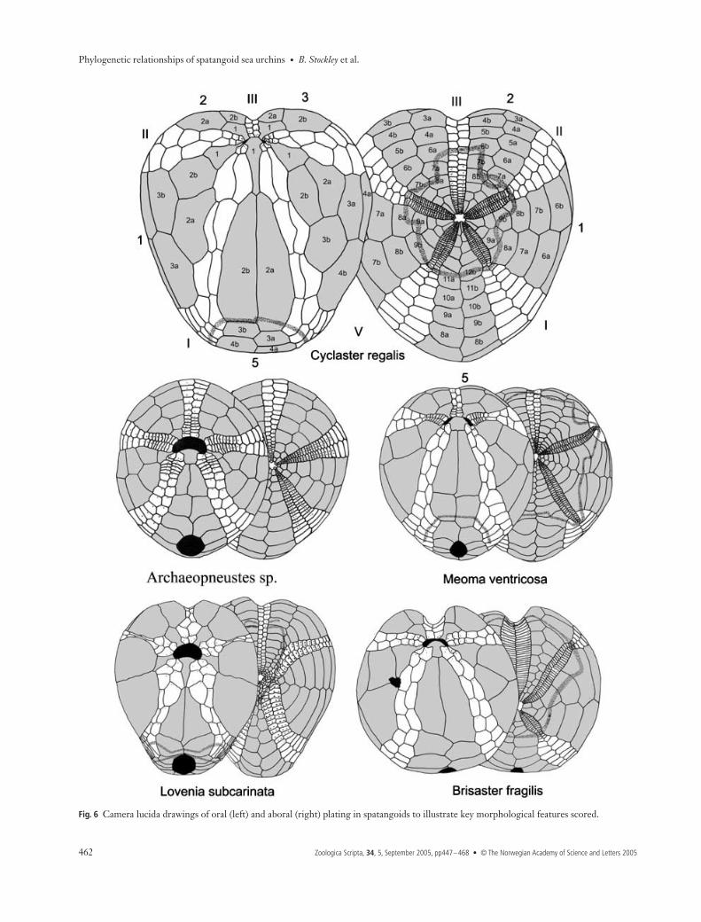
8-32. Ambulacral features8−10. The depth of the frontal ambulacrum There is consider-able variation in how wide and how deeply indented thefrontal ambulacrum is in spatangoids. Furthermore, the degreeto which the frontal ambulacrum is sunken usually variesbetween the apex and the peristome. In some spatangoids,such as Brissus (Fig. 6) the anterior ambulacrum is narrow andremains flush with adjacent interambulacral zones throughoutits length. In others, such as Brisaster (Fig. 6) the ambulacrumis wide and deeply sunken from apex to peristome. It is possibleto have ambulacrum III more strongly depressed adapicallythan at the ambitus. In Hemiaster, for example, the anteriorambulacrum is weakly but distinctly depressed adapically but
Fig. 5 A–K. Camera lucida drawings of apicaldisc plating in spatangoids. —A. Abatus (�);—B. Abatus (�); —C. Toxaaster; —D. Macraster;—E. Paleopneustes; —F. Plesiozonus; —G.Protenaster; —H. Plagiobrissus; —I. Plesiopatagus;—J. Ova; —K. Aceste.
B. Stockley et al. • Phylogenetic relationships of spatangoid sea urchins
© The Norwegian Academy of Science and Letters 2005 • Zoologica Scripta, 34, 5, September 2005, pp447–468 461
this groove shallows and disappears by the ambitus. In Moirathe frontal groove is very deep adapically and shallows mark-edly as it approaches the ambitus. By contrast, in Pericosmusthe frontal ambulacrum is almost flush adapically and gradu-ally increases in depth to the ambitus.
To encompass all this variation we use three characters,each given an initial weighting of 0.333 so that the structureof the frontal ambulacrum overall is equivalent to a singlecharacter in the analysis:8 Ambulacrum III midway between apex and ambitus: flush (0);shallowly concave (1); at least as deep as wide (2).9 Ambulacrum III at ambitus: flush so that ambitus appears flator convex in plan view (0); shallowly concave in plan view (1); atleast as deep as wide forming a prominent notch in plan view (2).10 Ambulacrum III on oral surface; flush (0); shallowly concavewith diffuse edges (1); forming a distinct channel with sharplydefined edges (2).11 Pore-pairs: small and undifferentiated adapically, their tube-feet simple and without suckers (0); differentiated adapically andassociated with enlarged funnel-building tube feet (1); laterallyelongate and subpetaloid, with specialized respiratory tube-feet (2).Adapical tube feet may be simple cylindrical structures or endin an enlarged disc. The latter are used by burrowing irregu-lar urchins to create and maintain a connection to the surfacethrough the sediment and may also be involved in selectingfood particles. In fossil taxa the size and morphology of theassociated pore-pairs in the frontal groove are used as a guideto whether adapical tube feet were specialized or not.
Only a few spatangoids have pore-pairs and tube feet of thefrontal ambulacrum identical to those in the paired ambu-lacra on the aboral surface. Occasionally, as in Isopneustes, allfive ambulacra are effectively petaloid and the pore-pairs inthe frontal ambulacrum are laterally elongate and identical inform to those in the paired ambulacra.12 Adapical tube feet of ambulacrum III: end in a blunt, rounded tip(0); penicillate (1); with wide flat-topped disc supported by a rosette ofplates (2). In most spatangoids aboral tube feet of ambulacrumIII lack skeletal elements in their tip. However, in a few taxaadapical tube feet are penicillate, ending in a mass of finger-likeextensions and are identical in form to the penicillate tube feetof the peristomial region. Each finger-like extension is sup-ported by a thin calcite rod. Other spatangoids have enlargedtube feet that end in an enlarged disc supported by a rosette-like ring of calcite platelets. Fossil taxa that have small undiffer-entiated pore-pairs are assumed to have simple tube feet.13 Frontal ambulacrum adapically: narrow, with pore-pairsclose together (ambulacral plates approximately as tall as wide) (0);moderately broadened with a distinct perradial zone (ambulacralplates 1.5−5× wider than tall — e.g. Brissopsis, Fig. 6) (1); verywide with ambulacral plates more than 5× wider than tall (2).This feature was measured on the aboral surface midwaybetween the apex and ambitus.
14 Pores: uniserial and uniform in frontal ambulacrum (0);biserially offset in adapical region (1); pore-pairs heterogeneous (2).Pores and tube feet in the frontal ambulacrum are generallyarranged in a single column adapically. However, in sometaxa tube feet can be crowded into the adapical region ofthe frontal ambulacra. In these forms the pores and tube feetbecome offset and biserially arranged. A few toxasteridshave two forms of pore-pair in their anterior ambulacrum,alternately narrow and elongate. This condition is scored asa third state.15 Lateral ambulacra (II and IV) on oral surface, wideningclose to peristome then narrowing markedly before broadening atambitus (pinched appearance): no (0); yes (1). The lateral ambu-lacral zones (II and IV) generally remain more or less parallel-sided as they approach the peristome or are only very slightlyenlarged (e.g. Archaeopneustes, Fig. 6). But in some maretiidsand loveniids (e.g. Lovenia, Fig. 6) these ambulacra becomestrongly pinched immediately distal to the phyllode zone.The ambulacra are scored as pinched if they reduce to lessthan half their width immediately before the phyllodes.16 Petal development: well developed with pores in each pairlarge and obvious and forming a pore-pair that is clearly laterallyelongate and supporting leaf-like tube-feet (0); small narrowpore-pairs supporting more or less cylindrical tube-feet (1); apetaloid— pores single and tube-feet microscopic (2).17 Petals: basically cruciform (0); anterior petals widely diverg-ing so as to be c. 180° (1); anterior petals flexed forwards so asto become subparallel to anterior ambulacrum (2). In regularechinoids the ambulacra radiate regularly with an angle of 72°between adjacent pairs. In spatangoids, the angle between theambulacra is more variable. Mostly anterior and posteriorpetals define an X-shaped pattern (e.g. Meoma, Fig. 6), butother patterns can be found. The anterior petals may divergeso widely that they define a nearly straight line (e.g. Brissus,Fig. 6), or they may be strongly flexed towards the anteriorand become subparallel. Petals are classed as state 1 if theangle between the anterior petals (measured from the tips tothe apical disc) is more than 160° and as state 2 if the angle isless than 50°.18 Anterior petals unequal in length: no (0); yes (1). The petalsof Nacospatangus are unusual in having one anterior petal(ambulacrum IV) substantially longer than the other. This isclearly a derived condition.19 In the anterior petals, the anterior column with about halfthe number of plates found in the posterior column: no (0); yes (1).Almost all spatangoids have a strict alternating one-to-onecorrespondence between the plates in the two columnsforming the ambulacra. The only exception to this patternis seen in the fossil taxa Heteraster and Washitaster, wherethe anterior column of the anterior petals is composed ofapproximately half the number of plates seen in the posteriorcolumn.
Phylogenetic relationships of spatangoid sea urchins • B. Stockley et al.
462 Zoologica Scripta, 34, 5, September 2005, pp447–468 • © The Norwegian Academy of Science and Letters 2005
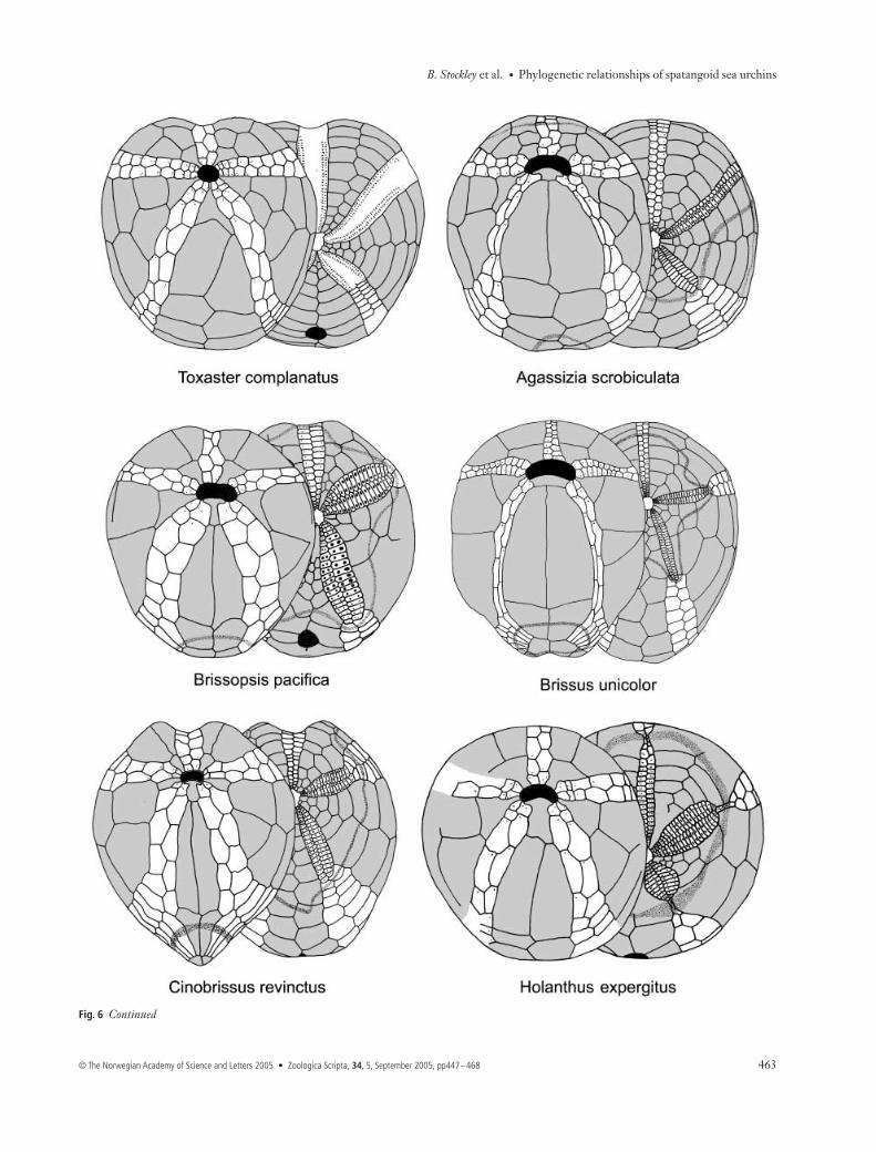
Fig. 6 Camera lucida drawings of oral (left) and aboral (right) plating in spatangoids to illustrate key morphological features scored.
B. Stockley et al. • Phylogenetic relationships of spatangoid sea urchins
© The Norwegian Academy of Science and Letters 2005 • Zoologica Scripta, 34, 5, September 2005, pp447–468 463
Fig. 6 Continued
Phylogenetic relationships of spatangoid sea urchins • B. Stockley et al.
464 Zoologica Scripta, 34, 5, September 2005, pp447–468 • © The Norwegian Academy of Science and Letters 2005
20 Anterior and posterior petal relative lengths: subequal (0);posterior petals between 0.5 and 0.7× length of anterior petals (1);posterior petals much shorter (less than half ) length of anterior petals(2); anterior petals distinctly shorter than posterior petals (< 0.8length) (3). There is great variability in the relative lengths ofthe posterior and anterior petals. Frequently, the posteriorpetals are shorter than the anterior petals (e.g. Agassizia,Fig. 6), sometimes substantially so (e.g. Brisaster, Fig. 6). It isalso possible for the anterior petals to be distinctly shorterthan the posterior petals (e.g. Cionobrissus, Fig. 6), or for thepetals to be subequal (e.g. Meoma, Fig. 6).21 Petals: flush (0); weakly depressed (1); deeply sunken andinvaginated (2). Petals can be flush on the surface of the test,or sunken to a greater or lesser extent, forming furrows on itssurface. In some Schizasteridae the petals can be even moredeeply sunken, forming a semi-enclosed cavity. Petals arescored as deeply sunken if their depth exceeds their width;they are found in the females of some sexually dimorphicspecies (e.g. Amphipneustes ) [char. 6]. In such sexually dimorphicforms the depth of petals is scored only for males so as toexclude brood chambers.22 Pores of Ib and IIa forming an arc laterally: no (0); yes (1). Inmany Loveniidae the petals are kinked adapically such thatthe lateral aboral interambulacral plates reduce substantiallyin size near the apical disc. This results in the pores in Ib andIIa forming an almost unbroken arc (e.g. Lovenia, Fig. 6).Although widely present in certain genera, this character isnot developed within all species and is very much dependentupon petal development. Scoring was based on the conditionshown in the adult type species.23 Anterior column of pore-pairs in frontal petals: rudimentarythroughout (0); developed only in distal half (1); developedthroughout almost their entire length, becoming rudimentary onlyas they approach the apex (2). Most spatangoids do not showsubstantial reduction of the pore-pairs in the anterior columnof the frontal petals (petals II and IV), or have only a minorasymmetry of development between anterior and posteriorcolumns. However, pore-pairs in this column can be rudi-mentary in their adapical portion (e.g. Lovenia, Fig. 6) orthroughout (e.g. Agassizia, Fig. 6).24 Petals end in occluded plates: no (0); yes (1). In many pale-opneustids and brissids the terminal plates of the petals arereduced and occluded from the adradial suture. The terminalplates of the petals are thus enclosed by the first ambulacralplates beyond the ends of the petals (e.g. Meoma, Fig. 6).More usually, all ambulacral plates meet the adradial sutureand there are no such occluded plates at the tips of petals (e.g.Cyclaster, Fig. 6).25 Ambulacral zone beneath the petal ends extremely pinched:no (0); yes (1). It is common for many spatangoids to show aslight reduction in the width of the ambulacral zones at theends of the petals. However, in a few taxa (e.g. Holanthus,
Fig. 6) the reduction that occurs is very marked, and theseplates are considerably less than a quarter of the width ofplates in the petals or plates further towards the ambitus.26 Distal termination of petals: the petal pore-pairs end abruptly(0); the petal pore-pairs decrease in size gradually and there is noabrupt end to the petals (1).27 Petal shape: the two columns parallel along their length (e.g.Meoma, Fig. 6) (0); petals lanceolate widened in the middle andconverging distally (e.g. Spatangus) (1); petals gradually wideningdistally (e.g. Archaeopneustes, Fig. 6) (2). We distinguish threebasic shapes of petals amongst spatangoids, as illustrated,according to whether the pore columns remain parallel, divergeor converge towards their tip.28 Anterior petal length: short, extending only about half thedistance to the ambitus (0); extending between 0.6 and 0.9 of theradial length (1); reaching the ambitus in plan view (2). Theradial extent of petals is quite variable, with some taxa havingpetaloid zones extending more or less to the ambitus whileothers have short petals that extend less than half the radialdistance to the ambitus. Although there seems to be more orless continuous graduation, it seems worth distinguishingforms with particularly short petals and those where the petalsextend more or less to the ambitus.29 Phyllode development in lateral paired ambulacra: phyllodepores/tube feet no more than 1 or 2 in a column (0); 4−7 in eachcolumn (1); 8−12 in each column (2); 13+ in each column (3).30 Pore-pairs in petals: the two columns closely spaced leavingalmost no perradial zone (0); separated by more than 1.5× the pore-pair width (1).31 Ambulacral plating becomes uniserial adapically: no (0); yes (1).In a few specialized deep-sea spatangoids the ambulacralplating becomes uniserial adapically, which is clearly aderived condition.32 Subanal tube feet enlarged and with disc: no (0); yes (1). Thepresence of enlarged subanal pore-pairs is used as evidencefor specialized tube feet in fossil taxa.
33-46. Interambulacral plating and plastron characters33 Number of ambulacral plate abutting rear suture of labralplate in ambulacrum I: 1 (0); 2 (1); 3 (2); 4+ (3). The suturebetween the labral plate and sternal plate 5.b.2 abuts againstambulacral plates of column Ia. Here we score the ambulacralplate, numbered from the peristome (see Fig. 6) that is mostcommonly present in this position in adults. However, therecan be a small amount of variation in this character withinpopulations, particularly where the number is large. Forexample Genicopatagus can have ambulacral plate 4 or 5abutting the rear of the labral plate.34 Number of ambulacral plate abutting rear suture of sternalplate in ambulacrum I : 5 (0); 6 (1); 7 or 8 (2); 9+ (3); 3 or 4 (4).This character, like char. 33, simply scores for the ambulacralplate, numbered from the peristome, that abuts the rear
B. Stockley et al. • Phylogenetic relationships of spatangoid sea urchins
© The Norwegian Academy of Science and Letters 2005 • Zoologica Scripta, 34, 5, September 2005, pp447–468 465
suture of sternal plate 5.b.2. In Micrasterina this is very con-sistent, and is always ambulacral plate 6. This is independentof char. 33. Note that in Paleopneustina it can be variablewithin species.35 Suture between labral and sternal plates: straight (0); stronglycurved (1). Whereas the suture between the labral plate andsternal plates in primitive spatangoids is strongly curved(convex towards the peristome), in derived spatangoids it ismore or less straight.36 Sternal plates, symmetrical with vertical median suture: no(0); yes (1). The two sternal plates are distinctly asymmetricalin primitive spatangoids (e.g. Toxaster, Fig. 6), with plate 2bwider anteriorly and plate 2a wider at the posterior. This isthe result of the median suture being strongly oblique. Inderived spatangoids the suture separating the two sternalplates is more or less vertical and the two plates mirrorimages of each other.37 Labral plate: in contact with both sternal plates (0); in contactwith only sternal plate 2b (1). There are relatively few spatangids,all within the family Somaliasteridae, where the labral plateis in contact with just a single sternal plate. This is presumablya derived condition.38 Labral plate, disjunct: no (0); yes (1).39 Episternals: biserially offset (0); paired and opposite (1).Schizasteridae, Toxasteridae and Hemiasteridae have biseri-ally offset episternal plates (e.g. Cyclaster, Fig. 6, plates 3a,3b). By contrast, in brissids and their close relatives, theepisternal plates are paired and opposite, and are mirrorimages of each other (e.g. Brissus, Fig. 6). The plates arescored as paired if the displacement between them behind thesternal plates is less than 10% of the total anterior−posteriorlength of the episternal plates.40 Sternal−episternal suture: approximately horizontal or V-dtowards posterior (0); significantly convex towards the peristome(1). Most spatangoids have approximately horizontal sternal−episternal sutures, whether the episternal plates are paired oroffset. However, in taxa where the episternal plates arepaired, this suture can be rather strongly flexed towards theperistome, as in Metalia and Plagiobrissus.41 Post-episternals: biserially offset (0); paired and weakly stag-gered (1); opposite (2). The staggering (or otherwise) of thesuture between the episternal plate (5.a/b.3) and the plate tothe rear (plate 5.a/b.4) often follows that of the episternal/sternal plates, but not always.42 Ambulacral plate series in columns Vb and Ia: undifferentiatedin subanal region (0); with marked change in shape of ambulacralplates such that they become transverse and geniculate behindthe episternal plates (1). In hemiasterids and toxasterids theposterior ambulacra do not vary in their overall shape orindent interambulacrum 5 on the oral surface (e.g. Toxaster,Fig. 6). However, in the Brissidae and Spatangidae, ambu-lacral plates change from being longitudinal to being laterally
enlarged, and ambulacral plate 6 in columns Ia and Vbindents the posterior interambulacrum to the rear of theepisternal plates (e.g. Cionobrissus, Fig. 6). This is associatedwith the development of a subanal fasciole and subanal tubefeet, but still occurs where the subanal fasciole has beensecondarily lost.43 Lateral paired interambulacra: both amphiplacous (0); onemeridoplacous, one amphiplacous (1); both meridoplacous (2). Inamphiplacous taxa the first adoral interambulacral plateabuts against two plates (e.g. Holanthus, Fig. 6), whereas inmeridoplacous taxa it abuts distally against a single plate(e.g. Cionobrissus, Fig. 6). In some taxa both left and rightinterambulacra are meridoplacous, whereas in others thedevelopment is asymmetrical, with interambulacrum 1amphiplacous and interambulacrum 5 meridoplacous (e.g.Cyclaster, Fig. 6).44 Plastron: widening to the rear (0); more or less parallel-sided,not narrowing markedly to rear of episternal plates (e.g. Brissopsis,Fig. 6) (1); strongly tapered to rear of episternal plates which makeonly a narrow contact with interambulacral plates to the posterior(e.g. Cionobrissus, Fig. 6) (2).45 Lateral interambulaca on oral surface: comprise at least four orfive plates (0); composed of just the basicoronal plate and the twosucceeding plates (plates 2a, 2b) (1); as 1 but these plates flat so thatthe oral surface is planar (2).46 Length of labrum: much smaller than sternal plates (0); 20−50% length of sternal plates (1); more than 50% of sternal platesin length (2). [ordered]
47-53. Peristome and periproct47 Peristome position: closer to the anterior border than the centre(0); subcentral (1). Although almost all spatangoids have theperistome opening some 10−20% test length from the anteriorthere are a few taxa that have a more subcentral peristome. Asubcentral peristome is also the condition seen in most primitiveirregular echinoids although not in the immediate outgroup.The peristome is scored as subcentral if its anterior border iscloser to the midlength of the test than the anterior border.48 Peristome shape: circular to ovate (0); distinctly pentagonal andangular (1).49 Peristome orientation: downward-facing; circular or pen-tagonal without labral plate projecting below the plane of the open-ing (0); obliquely facing forwards (labral plate strongly projectingso that peristome appears C-shaped) (1); peristome vertical andalmost entirely hidden in plan view by the labral plate (2). Theorientation of the peristome and the degree to which thelabral plate covers the opening in oral view is a continuousvariable that is here divided into three states. In many EarlyCretaceous forms the peristome is a simple circular topentagonal opening that faces directly downwards and theposterior boundary is straight or convex to the rear. However,in the majority of living forms the labral plate projects to a
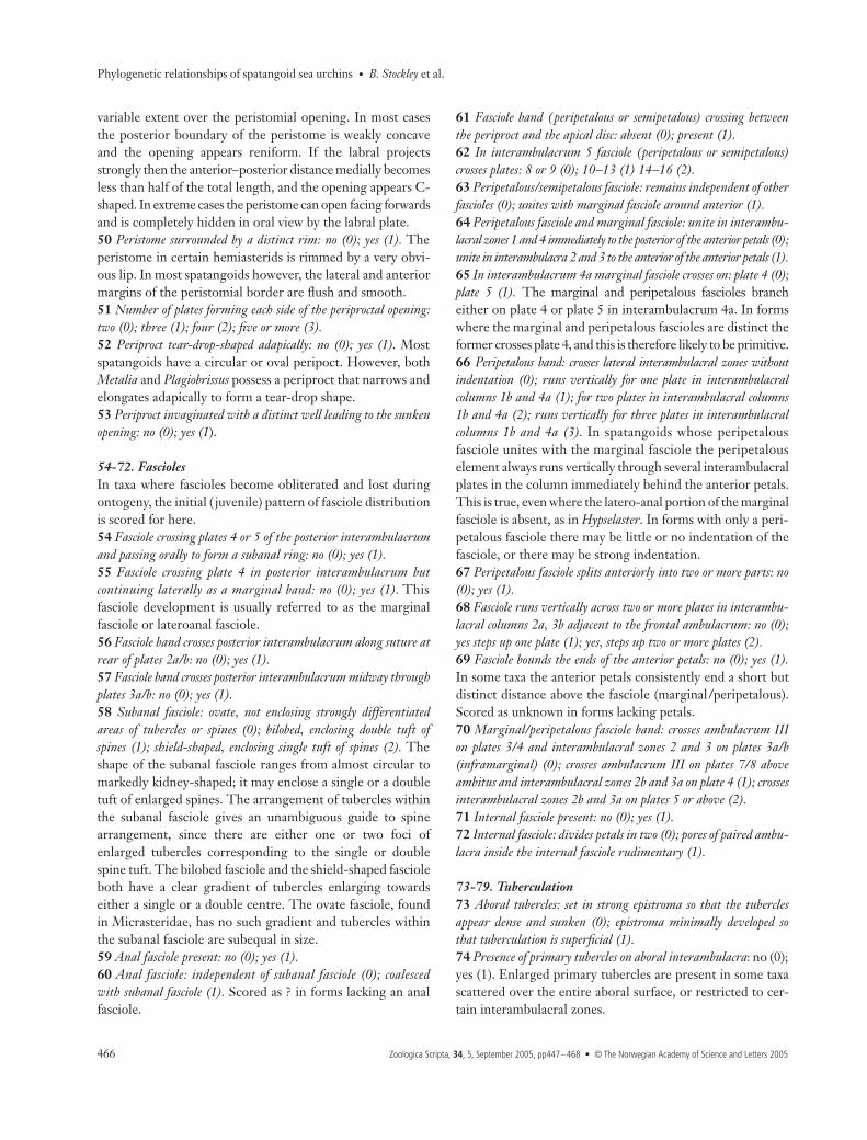
Phylogenetic relationships of spatangoid sea urchins • B. Stockley et al.
466 Zoologica Scripta, 34, 5, September 2005, pp447–468 • © The Norwegian Academy of Science and Letters 2005
variable extent over the peristomial opening. In most casesthe posterior boundary of the peristome is weakly concaveand the opening appears reniform. If the labral projectsstrongly then the anterior−posterior distance medially becomesless than half of the total length, and the opening appears C-shaped. In extreme cases the peristome can open facing forwardsand is completely hidden in oral view by the labral plate.50 Peristome surrounded by a distinct rim: no (0); yes (1). Theperistome in certain hemiasterids is rimmed by a very obvi-ous lip. In most spatangoids however, the lateral and anteriormargins of the peristomial border are flush and smooth.51 Number of plates forming each side of the periproctal opening:two (0); three (1); four (2); five or more (3).52 Periproct tear-drop-shaped adapically: no (0); yes (1). Mostspatangoids have a circular or oval peripoct. However, bothMetalia and Plagiobrissus possess a periproct that narrows andelongates adapically to form a tear-drop shape.53 Periproct invaginated with a distinct well leading to the sunkenopening: no (0); yes (1).
54-72. FasciolesIn taxa where fascioles become obliterated and lost duringontogeny, the initial ( juvenile) pattern of fasciole distributionis scored for here.54 Fasciole crossing plates 4 or 5 of the posterior interambulacrumand passing orally to form a subanal ring: no (0); yes (1).55 Fasciole crossing plate 4 in posterior interambulacrum butcontinuing laterally as a marginal band: no (0); yes (1). Thisfasciole development is usually referred to as the marginalfasciole or lateroanal fasciole.56 Fasciole band crosses posterior interambulacrum along suture atrear of plates 2a/b: no (0); yes (1).57 Fasciole band crosses posterior interambulacrum midway throughplates 3a/b: no (0); yes (1).58 Subanal fasciole: ovate, not enclosing strongly differentiatedareas of tubercles or spines (0); bilobed, enclosing double tuft ofspines (1); shield-shaped, enclosing single tuft of spines (2). Theshape of the subanal fasciole ranges from almost circular tomarkedly kidney-shaped; it may enclose a single or a doubletuft of enlarged spines. The arrangement of tubercles withinthe subanal fasciole gives an unambiguous guide to spinearrangement, since there are either one or two foci ofenlarged tubercles corresponding to the single or doublespine tuft. The bilobed fasciole and the shield-shaped fascioleboth have a clear gradient of tubercles enlarging towardseither a single or a double centre. The ovate fasciole, foundin Micrasteridae, has no such gradient and tubercles withinthe subanal fasciole are subequal in size.59 Anal fasciole present: no (0); yes (1).60 Anal fasciole: independent of subanal fasciole (0); coalescedwith subanal fasciole (1). Scored as ? in forms lacking an analfasciole.
61 Fasciole band ( peripetalous or semipetalous) crossing betweenthe periproct and the apical disc: absent (0); present (1).62 In interambulacrum 5 fasciole (peripetalous or semipetalous)crosses plates: 8 or 9 (0); 10−13 (1) 14−16 (2).63 Peripetalous/semipetalous fasciole: remains independent of otherfascioles (0); unites with marginal fasciole around anterior (1).64 Peripetalous fasciole and marginal fasciole: unite in interambu-lacral zones 1 and 4 immediately to the posterior of the anterior petals (0);unite in interambulacra 2 and 3 to the anterior of the anterior petals (1).65 In interambulacrum 4a marginal fasciole crosses on: plate 4 (0);plate 5 (1). The marginal and peripetalous fascioles brancheither on plate 4 or plate 5 in interambulacrum 4a. In formswhere the marginal and peripetalous fascioles are distinct theformer crosses plate 4, and this is therefore likely to be primitive.66 Peripetalous band: crosses lateral interambulacral zones withoutindentation (0); runs vertically for one plate in interambulacralcolumns 1b and 4a (1); for two plates in interambulacral columns1b and 4a (2); runs vertically for three plates in interambulacralcolumns 1b and 4a (3). In spatangoids whose peripetalousfasciole unites with the marginal fasciole the peripetalouselement always runs vertically through several interambulacralplates in the column immediately behind the anterior petals.This is true, even where the latero-anal portion of the marginalfasciole is absent, as in Hypselaster. In forms with only a peri-petalous fasciole there may be little or no indentation of thefasciole, or there may be strong indentation.67 Peripetalous fasciole splits anteriorly into two or more parts: no(0); yes (1).68 Fasciole runs vertically across two or more plates in interambu-lacral columns 2a, 3b adjacent to the frontal ambulacrum: no (0);yes steps up one plate (1); yes, steps up two or more plates (2).69 Fasciole bounds the ends of the anterior petals: no (0); yes (1).In some taxa the anterior petals consistently end a short butdistinct distance above the fasciole (marginal/peripetalous).Scored as unknown in forms lacking petals.70 Marginal/peripetalous fasciole band: crosses ambulacrum IIIon plates 3/4 and interambulacral zones 2 and 3 on plates 3a/b(inframarginal) (0); crosses ambulacrum III on plates 7/8 aboveambitus and interambulacral zones 2b and 3a on plate 4 (1); crossesinterambulacral zones 2b and 3a on plates 5 or above (2).71 Internal fasciole present: no (0); yes (1).72 Internal fasciole: divides petals in two (0); pores of paired ambu-lacra inside the internal fasciole rudimentary (1).
73-79. Tuberculation73 Aboral tubercles: set in strong epistroma so that the tuberclesappear dense and sunken (0); epistroma minimally developed sothat tuberculation is superficial (1).74 Presence of primary tubercles on aboral interambulacra: no (0);yes (1). Enlarged primary tubercles are present in some taxascattered over the entire aboral surface, or restricted to cer-tain interambulacral zones.
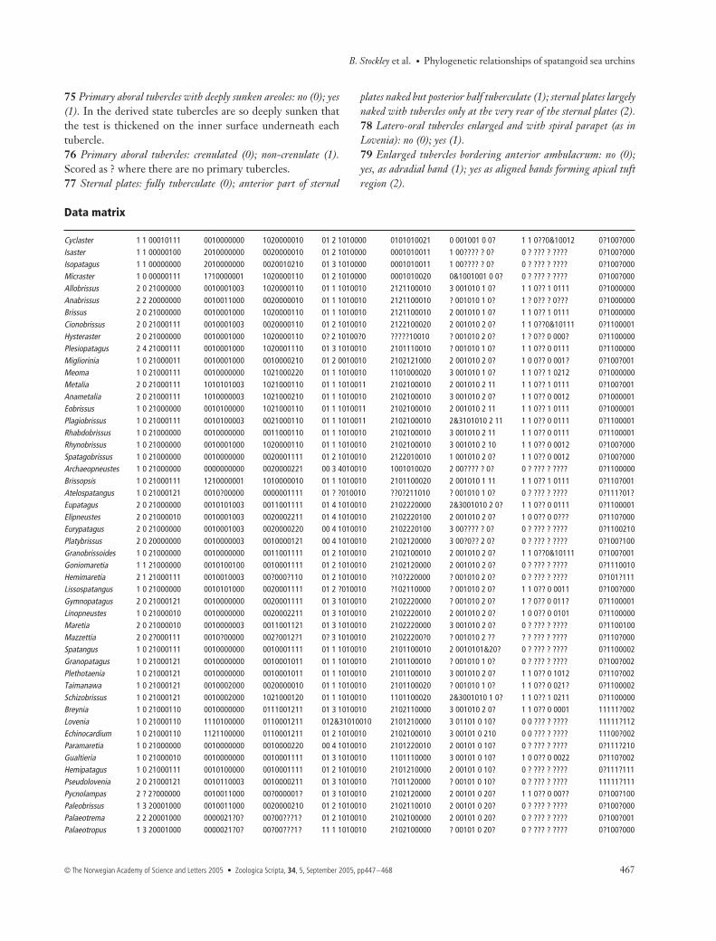
B. Stockley et al. • Phylogenetic relationships of spatangoid sea urchins
© The Norwegian Academy of Science and Letters 2005 • Zoologica Scripta, 34, 5, September 2005, pp447–468 467
75 Primary aboral tubercles with deeply sunken areoles: no (0); yes(1). In the derived state tubercles are so deeply sunken thatthe test is thickened on the inner surface underneath eachtubercle.76 Primary aboral tubercles: crenulated (0); non-crenulate (1).Scored as ? where there are no primary tubercles.77 Sternal plates: fully tuberculate (0); anterior part of sternal
plates naked but posterior half tuberculate (1); sternal plates largelynaked with tubercles only at the very rear of the sternal plates (2).78 Latero-oral tubercles enlarged and with spiral parapet (as inLovenia): no (0); yes (1).79 Enlarged tubercles bordering anterior ambulacrum: no (0);yes, as adradial band (1); yes as aligned bands forming apical tuftregion (2).
Data matrix
Cyclaster 1 1 00010111 0010000000 1020000010 01 2 1010000 0101010021 0 001001 0 0? 1 1 0??0&10012 0?100?000Isaster 1 1 00000100 2010000000 0020000010 01 2 1010000 0001010011 1 00???? ? 0? 0 ? ??? ? ???? 0?100?000Isopatagus 1 1 00000000 2010000000 0020010210 01 3 1010000 0001010011 1 00???? ? 0? 0 ? ??? ? ???? 0?100?000Micraster 1 0 00000111 1?10000001 1020000110 01 2 1010000 0001010020 0&1001001 0 0? 0 ? ??? ? ???? 0?100?000Allobrissus 2 0 21000000 0010001003 1020000110 01 1 1010010 2121100010 3 001010 1 0? 1 1 0?? 1 0111 0?1000000Anabrissus 2 2 20000000 0010011000 0020000010 01 1 1010010 2121100010 ? 001010 1 0? 1 ? 0?? ? 0??? 0?1000000Brissus 2 0 21000000 0010001000 1020000110 01 1 1010010 2121100010 2 001010 1 0? 1 1 0?? 1 0111 0?1000000Cionobrissus 2 0 21000111 0010001003 0020000110 01 2 1010010 2122100020 2 001010 2 0? 1 1 0??0&10111 0?1100001Hysteraster 2 0 21000000 0010001000 1020000110 0? 2 10100?0 ?????10010 ? 001010 2 0? 1 ? 0?? 0 000? 0?1100000Plesiopatagus 2 4 21000111 0010001000 1020001110 01 3 1010010 2101110010 ? 001010 1 0? 1 1 0?? 0 0111 0?1100000Migliorinia 1 0 21000011 0010001000 0010000210 01 2 0010010 2102121000 2 001010 2 0? 1 0 0?? 0 001? 0?100?001Meoma 1 0 21000111 0010000000 1021000220 01 1 1010010 1101000020 3 001010 1 0? 1 1 0?? 1 0212 0?1000000Metalia 2 0 21000111 1010101003 1021000110 01 1 1010011 2102100010 2 001010 2 11 1 1 0?? 1 0111 0?100?001Anametalia 2 0 21000111 1010000003 1021000210 01 1 1010010 2102100010 3 001010 2 0? 1 1 0?? 0 0012 0?1000001Eobrissus 1 0 21000000 0010100000 1021000110 01 1 1010011 2102100010 2 001010 2 11 1 1 0?? 1 0111 0?1000001Plagiobrissus 1 0 21000111 0010100003 0021000110 01 1 1010011 2102100010 2&3101010 2 11 1 1 0?? 0 0111 0?1100001Rhabdobrissus 1 0 21000000 0010000000 0011000110 01 1 1010010 2102100010 3 001010 2 11 1 1 0?? 0 0111 0?1100001Rhynobrissus 1 0 21000000 0010001000 1020000110 01 1 1010010 2102100010 3 001010 2 10 1 1 0?? 0 0012 0?100?000Spatagobrissus 1 0 21000000 0010000000 0020001111 01 2 1010010 2122010010 1 001010 2 0? 1 1 0?? 0 0012 0?100?000Archaeopneustes 1 0 21000000 0000000000 0020000221 00 3 4010010 1001010020 2 00???? ? 0? 0 ? ??? ? ???? 0?1100000Brissopsis 1 0 21000111 1210000001 1010000010 01 1 1010010 2101100020 2 001010 1 11 1 1 0?? 1 0111 0?110?001Atelospatangus 1 0 21000121 0010?00000 0000001111 01 ? ?010010 ??0?211010 ? 001010 1 0? 0 ? ??? ? ???? 0?111?01?Eupatagus 2 0 21000000 0010101003 0011001111 01 4 1010010 2102220000 2&3001010 2 0? 1 1 0?? 0 0111 0?1100001Elipneustes 2 0 21000010 0010001003 0020002211 01 4 1010010 2102220100 2 001010 2 0? 1 0 0?? 0 0??? 0?110?000Eurypatagus 2 0 21000000 0010001003 0020000220 00 4 1010010 2102220100 3 00???? ? 0? 0 ? ??? ? ???? 0?1100210Platybrissus 2 0 20000000 0010000003 0010000121 00 4 1010010 2102120000 3 00?0?? 2 0? 0 ? ??? ? ???? 0?100?100Granobrissoides 1 0 21000000 0010000000 0011001111 01 2 1010010 2102100010 2 001010 2 0? 1 1 0??0&10111 0?100?001Goniomaretia 1 1 21000000 0010100100 0010001111 01 2 1010010 2102120000 2 001010 2 0? 0 ? ??? ? ???? 0?1110010Hemimaretia 2 1 21000111 0010010003 00?000?110 01 2 1010010 ?10?220000 ? 001010 2 0? 0 ? ??? ? ???? 0?101?111Lissospatangus 1 0 21000000 0010101000 0020001111 01 2 ?010010 ?102110000 ? 001010 2 0? 1 1 0?? 0 0011 0?100?000Gymnopatagus 2 0 21000121 0010000000 0020001111 01 3 1010010 2102220000 ? 001010 2 0? 1 ? 0?? 0 011? 0?1100001Linopneustes 1 0 21000010 0010000000 0020002211 01 3 1010010 2102220010 2 001010 2 0? 1 0 0?? 0 0101 0?1100000Maretia 2 0 21000010 0010000003 0011001121 01 3 1010010 2102220000 3 001010 2 0? 0 ? ??? ? ???? 0?1100100Mazzettia 2 0 2?000111 0010?00000 002?0012?1 0? 3 1010010 21022200?0 ? 001010 2 ?? ? ? ??? ? ???? 0?110?000Spatangus 1 0 21000111 0010000000 0010001111 01 1 1010010 2101100010 2 0010101&20? 0 ? ??? ? ???? 0?1100002Granopatagus 1 0 21000121 0010000000 0010001011 01 1 1010010 2101100010 ? 001010 1 0? 0 ? ??? ? ???? 0?100?002Plethotaenia 1 0 21000121 0010000000 0010001011 01 1 1010010 2101100010 3 001010 2 0? 1 1 0?? 0 1012 0?110?002Taimanawa 1 0 21000121 0010002000 0020000010 01 1 1010010 2101100020 ? 001010 1 0? 1 1 0?? 0 021? 0?1100002Schizobrissus 1 0 21000121 0010002000 1021000120 01 1 1010010 1101100020 2&3001010 1 0? 1 1 0?? 1 0211 0?1100000Breynia 1 0 21000110 0010000000 0111001211 01 3 1010010 2102110000 3 001010 2 0? 1 1 0?? 0 0001 11111?002Lovenia 1 0 21000110 1110100000 0110001211 012&31010010 2101210000 3 01101 0 10? 0 0 ??? ? ???? 11111?112Echinocardium 1 0 21000110 1121100000 0110001211 01 2 1010010 2102100010 3 00101 0 210 0 0 ??? ? ???? 11100?002Paramaretia 1 0 21000000 0010000000 0010000220 00 4 1010010 2101220010 2 00101 0 10? 0 ? ??? ? ???? 0?111?210Gualtieria 1 0 21000010 0010000000 0010001111 01 3 1010010 1101110000 3 00101 0 10? 1 0 0?? 0 0022 0?110?002Hemipatagus 1 0 21000111 0010100000 0010001111 01 2 1010010 2101210000 2 00101 0 10? 0 ? ??? ? ???? 0?111?111Pseudolovenia 2 0 21000121 0010110003 0010000211 01 3 1010010 ?101120000 ? 00101 0 10? 0 ? ??? ? ???? 11111?111Pycnolampas 2 ? 2?000000 0010011000 00?000001? 01 3 1010010 2102120000 2 00101 0 20? 1 1 0?? 0 00?? 0?100?100Paleobrissus 1 3 20001000 0010011000 0020000210 01 2 1010010 2102110010 2 00101 0 20? 0 ? ??? ? ???? 0?100?000Palaeotrema 2 2 20001000 0000021?0? 00?00???1? 01 2 1010010 2102100000 2 00101 0 20? 0 ? ??? ? ???? 0?100?001Palaeotropus 1 3 20001000 0000021?0? 00?00???1? 11 1 1010010 2102100000 ? 00101 0 20? 0 ? ??? ? ???? 0?100?000
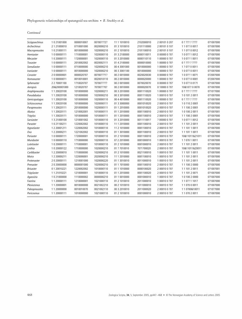
Phylogenetic relationships of spatangoid sea urchins • B. Stockley et al.
468 Zoologica Scripta, 34, 5, September 2005, pp447–468 • © The Norwegian Academy of Science and Letters 2005
Scrippsechinus 1 0 21001000 000001000? 00?00???2? 11 1 1010010 2102000010 2 00101 0 20? 0 ? ??? ? ???? 0?100?000Archechinus 2 1 21000010 0?10001000 0020000210 01 3 1010010 2101110000 2 00101 0 10? 1 1 0?? 0 001? 0?100?000Macropneustes 1 0 21000111 0010000000 1020000210 01 2 1010010 2101100010 2 00101 0 10? 1 1 0?? 0 0012 0?100?000Hemiaster 1 0 00000111 1?10000001 1020000110 01 3 2100000 0000110011 0 00000 0 ?0? 1 0 0?? 1 0012 0?100?000Mecaster 1 0 20000111 1?20000001 1020000110 01 3 2010000 0000110110 1 00000 0 ?0? 1 0 0?? 1 0011 0?100?000Toxaster 1 0 00000111 2010002002 0020002111 01 4 2100000 0000010000 1 00000 0 ?0? 0 ? ??? ? ???? 0?100?000Somaliaster 1 0 00000111 0?10000000 1020000210 00 4 3001000 0010000000 1 00000 0 ?0? 1 ? 0?? 0 0011 0?100?000Iraniaster 1 0 00000111 0010000000 1020000210 00 3 3001100 0010000000 1 00000 0 ?0? 1 0 0?? 0 0011 0?100?000Coraster 2 0 00000001 0000020?0? 00?00???1? 00 2 0010000 0020020030 0 00000 0 ?0? 1 0 0?? 1 00?1 0?200?000Homoeaster 1 0 00000011 0010010001 0020010110 00 2 0010000 0000020000 1 00000 0 ?0? 1 0 0?? 0 0001 0?200?000Sphenaster 2 2 ?0001100 1?10020?0? ?0?00????? 00 2 0010000 00?00200?0 0 00000 0 ?0? 1 0 0?? 0 01?1 0?100?000Aeropsis 20&200001000 1210020?0? ?0?00???0? 00 2 0010000 00000200?0 0 10000 0 ?0? 10&10?? 0 00?0 0?100?000Amphipneustes 1 1 20020100 1010000000 1020000211 00 3 2010000 0001110020 1 00000 0 ?0? 0 ? ??? ? ???? 0?10??000Pseudabatus 1 1 20020100 1010000000 1020000210 00 3 3010000 0001110020 1 00010 0 ?0? 1 0 101 2 0011 0?100?000Genicopatagus 1 1 20020100 1010000000 1020000110 00 4 4010000 0001110020 1 00000 0 ?0? 0 ? ??? ? ???? 0?100?000Schizocosmus 1 1 20020100 1010000000 1020000111 01 3 3000000 0001010020 2 00010 0 ?0? 1 0 110 2 0001 0?100?000Parapneustes 1 1 20020111 2010000000 1020000111 01 1 2010000 0001010020 2 00010 0 ?0? 1 1 100 2 0001 0?100?000Abatus 1 1 20020111 1210002001 1010000111 01 1 2010000 0001100010 2 00010 0 ?0? 1 0 100 2 0011 0?100?001Tripylus 1 1 20020111 1010000000 1010000111 01 1 2010000 0001100010 2 00010 0 ?0? 1 1 100 2 0001 0?100?000Sarsiaster 1 3 21000100 1210001002 1010000110 01 3 2010000 001111001? ? 00000 0 ?0? 1 0 0?? 1 0012 0?100?000Paraster 1 0 21100211 1220002002 1010000110 11 1 2010000 0001100010 2 00010 0 ?0? 1 1 101 2 0011 0?100?000Hypselaster 1 2 20001211 1220002002 1010000110 11 2 1010000 0001100010 2 00010 0 ?0? 1 1 101 1 0011 0?100?000Ova 1 2 20000211 1221002002 1010000110 01 1 3010000 0001100010 2 00010 0 ?0? 1 1 101 1 0011 0?100?000Periaster 1 0 00000111 1?20000001 1010000110 01 2 1010000 0001100010 2 00010 0 ?0? 10&11011&21011 0?100?000Mundaster 1 0 00000110 1?10000000 1020000110 0? 2 2010000 0001000010 1 00010 0 ?0? 1 ? 0?0 1 0011 0?100?000Lutetiaster 1 0 20000111 1?10000001 1010000110 01 2 1010000 0001000010 2 00010 0 ?0? 1 1 101 2 0011 0?100?000Linthia 1 0 20000122 1?10000000 1020000210 01 ? ?010010 ?0?1?00020 2 00010 0 ?0? 10&11011&20011 0?100?000Caribbaster 1 2 20000010 1?10000000 1020000210 01 2 1010000 0021100010 1 00010 0 ?0? 1 1 101 1 0011 0?100?000Moira 1 2 20000211 1220000001 2020000210 11 1 2010000 0001100010 1 00010 0 ?0? 1 1 101 2 0011 0?100?000Protenaster 2 0 20000111 1210001000 1020000220 01 1 3010010 0011000010 1 00010 0 ?0? 1 1 101 2 0011 0?100?000Prenaster 2 0 20000000 0000001000 1020000210 01 1 ?010000 0001100010 2 00010 0 ?0? 1 1 100 2 0000 0?100?000Brisaster 0 1 20010221 1220002002 1010000110 01 1 1010000 0000100020 2 00010 0 ?0? 1 1 101 2 0011 0?100?001Tripylaster 1 1 21010221 1210000001 1010000110 01 1 2010000 0001100020 2 00010 0 ?0? 1 1 101 2 00?1 0?100?000Agassizia 1 0 21000000 1110000002 0000000210 01 1 0010000 0001000010 1 00010 0 ?0? 1 0 100 2 0000 0?100?000Faorina 1 1 20000111 1210000001 1021000110 01 2 1010010 2011000010 1 00010 0 ?0? 1 1 0?? 1 101? 0?100?000Plesiozonus 1 1 20000001 0010000000 0021002210 00 2 1010010 1011000010 1 00010 0 ?0? 1 1 0?0 0 0011 0?100?000Paleopneustes 1 1 20000000 00100100?0 0021002110 00 3 2010010 2011000020 2 00010 0 ?0? 1 1 0?00&10011 0?10??000Pericosmus 1 1 20000111 1010000000 1021000110 01 2 1010010 0001000010 2 00010 0 ?0? 1 1 0?0 2 0011 0?100?000
Continued
Related Documents


![9. Verletzungen und Vergiftungen durch Meerestiere · Seite: 6 Verletzungen und Vergiftungen durch Meerestiere Kapitel 9 Giftige Lederseeigel [poisonous urchins, Echinoidea] Im Gegensatz](https://static.cupdf.com/doc/110x72/5e07c10f5a73d95aba429ae6/9-verletzungen-und-vergiftungen-durch-meerestiere-seite-6-verletzungen-und-vergiftungen.jpg)