Photometry and Spectroscopy of GRB 030329 and Its Associated Supernova 2003dh: The First Two Months

arX

iv:a

stro

-ph/

0307

435v

2 2

5 A

ug 2

003

Photometry and Spectroscopy of GRB 030329 and Its Associated

Supernova 2003dh: The First Two Months

T. Matheson1, P. M. Garnavich2, K. Z. Stanek1, D. Bersier1, S. T. Holland2,3,

K. Krisciunas4,5, N. Caldwell1, P. Berlind6, J. S. Bloom1, M. Bolte7, A. Z. Bonanos1,

M. J. I. Brown8, W. R. Brown1, M. L. Calkins6, P. Challis1, R. Chornock9, L. Echevarria10,

D. J. Eisenstein11, M. E. Everett12, A. V. Filippenko9, K. Flint13, R. J. Foley9,

D. L. Freedman1, Mario Hamuy14, P. Harding15, N. P. Hathi10, M. Hicken1, C. Hoopes16,

C. Impey11, B. T. Jannuzi8, R. A. Jansen10, S. Jha9, J. Kaluzny17, S. Kannappan18,

R. P. Kirshner1, D. W. Latham1, J. C. Lee11, D. C. Leonard19, W. Li9, K. L. Luhman1,

P. Martini14, H. Mathis8, J. Maza20, S. T. Megeath1, L. R. Miller8, D. Minniti21,

E. W. Olszewski11, M. Papenkova9, M. M. Phillips4, B. Pindor22, D. D. Sasselov1,

R. Schild1, H. Schweiker23, T. Spahr1, J. Thomas-Osip4, I. Thompson14, D. Weisz9,

R. Windhorst10, and D. Zaritsky11

1Harvard-Smithsonian Center for Astrophysics, 60 Garden Street, Cambridge, MA 021382Dept. of Physics, University of Notre Dame, 225 Nieuwland Science Hall, Notre Dame, IN 465563Current Address: Goddard Space Flight Center, Code 662.20, Greenbelt, MD, 20771-00034Carnegie Institution of Washington, Las Campanas Observatory, Casilla 601, La Serena, Chile5Cerro Tololo Inter-American Observatory, Casilla 603, La Serena, Chile6F. L. Whipple Observatory, 670 Mt. Hopkins Road, P.O. Box 97, Amado, AZ 856457University of California Observatories/Lick Observatory, University of California, Santa Cruz, Santa

Cruz, CA 95064

8National Optical Astronomy Observatory, 950 North Cherry Ave., Tucson, AZ 857199University of California, Dept. of Astronomy, 601 Campbell Hall, Berkeley CA, 94720-3411

10Dept. of Physics and Astronomy, Arizona State University, Tempe, AZ 85287-150411Steward Observatory, University of Arizona, 933 N. Cherry Ave., Tucson, AZ 8571812Planetary Sciences Institute, 620 N. Sixth Avenue, Tucson, Arizona 8570513Carnegie Institution of Washington, DTM, 5241 Broad Branch Road, NW Washington, DC 2001514Carnegie Observatories, 813 Santa Barbara Street, Pasadena, CA 9110115Dept. of Astronomy, Case Western Reserve University, 10900 Euclid Avenue, Cleveland, OH 4410616Dept. of Physics and Astronomy, Johns Hopkins University, 3400 N. Charles St., Baltimore, MD 2121817Copernicus Astronomical Center, Bartycka 18, PL-00-716, Warsaw, Poland18The University of Texas at Austin, McDonald Obs., 1 University Station C1402, Austin, TX 78712-025919Five College Astronomy Department, University of Massachusetts, Amherst, MA 01003-930520Universidad de Chile, Casilla 36-D, Santiago, Chile21Pontificia Universidad Catolica de Chile, Casilla 306, Santiago, 22, Chile22Princeton University Observatory, Princeton, NJ 0854423WIYN Consortium Inc., 950 N Cherry Ave., Tucson, AZ 85719

http://arXiv.org/abs/astro-ph/0307435v2

– 2 –

[email protected], [email protected], [email protected],

[email protected], [email protected],













[email protected], [email protected], [email protected], [email protected],




[email protected], [email protected], [email protected]

ABSTRACT

We present extensive optical and infrared photometry of the afterglow of

gamma-ray burst (GRB) 030329 and its associated supernova (SN) 2003dh over

the first two months after detection (2003 March 30-May 29 UT). Optical spec-

troscopy from a variety of telescopes is shown and, when combined with the

photometry, allows an unambiguous separation between the afterglow and super-

nova contributions. The optical afterglow of the GRB is initially a power-law

continuum but shows significant color variations during the first week that are

unrelated to the presence of a supernova. The early afterglow light curve also

shows deviations from the typical power-law decay. A supernova spectrum is

first detectable ∼ 7 days after the burst and dominates the light after ∼ 11 days.

The spectral evolution and the light curve are shown to closely resemble those of

SN 1998bw, a peculiar Type Ic SN associated with GRB 980425, and the time of

the supernova explosion is close to the observed time of the GRB. It is now clear

that at least some GRBs arise from core-collapse SNe.

Subject headings: galaxies: distances and redshifts — gamma-rays: bursts —

supernovae: general — supernovae: individual (SN 2003dh)

– 3 –

1. Introduction

The mechanism that produces gamma-ray bursts (GRBs) has been the subject of consid-

erable speculation during the four decades since their discovery (see Meszaros 2002 for a re-

cent review of the theories of GRBs). The discovery of optical afterglows (e.g., GRB 970228:

Groot et al. 1997; van Paradijs et al. 1997) opened a new window on the field (see, e.g.,

van Paradijs, Kouveliotou, & Wijers 2000). Subsequent studies of other bursts yielded the

redshifts of several GRBs (e.g., GRB 970508: Metzger et al. 1997), providing definitive evi-

dence for their cosmological origin. Observations at other wavelengths, especially radio, have

revealed many more details about the bursts (e.g., Berger et al. 2000; Frail et al. 2003).

Models that invoked supernovae (SNe) to explain GRBs were proposed from the very

beginning (e.g., Colgate 1968; Woosley 1993; Woosley & MacFadyen 1999). There have

been tantalizing observational clues that also pointed to SNe as a possible mechanism for

producing GRBs. The most direct was GRB 980425: no traditional GRB optical afterglow

was seen, but a supernova, SN 1998bw, was found in the error box of the GRB (Galama et

al. 1998a). The SN was classified as a Type Ic (Patat & Piemonte 1998), but it was unusual,

with high expansion velocities (Patat et al. 2001). Other SNe with high expansion velocities

(and usually large luminosity as well) such as SN 1997ef and SN 2002ap are sometimes

referred to as “hypernovae” (see, e.g., Iwamoto et al. 1998, 2000). GRB 980425 was also

unusual in the sense that the isotropic energy of the burst was 10−3 to 10−4 times weaker

than in classical cosmological GRBs (Woosley, Eastman, & Schmidt 1999), indicating that

this was not a typical burst.

Indirect evidence also relates GRBs to SNe. Core-collapse SNe are associated with mas-

sive stars (e.g., Van Dyk, Hamuy, & Filippenko 1996) and GRBs also appear to be associated

with massive stars, based on their location in their host galaxies (e.g., Bloom, Kulkarni, &

Djorgovski 2002) and statistics of the types of galaxies that host GRBs (e.g., Hogg & Fruchter

1999). Chevalier & Li (2000) have shown that the afterglow properties of some GRBs are

consistent with a shock moving into a stellar wind formed from a massive star.

The redshift of a typical GRB is z ≈ 1, implying that a supernova component underlying

an optical afterglow would be difficult to detect. At z ≈ 1, even a bright core-collapse event

would peak at R > 23 mag. Nevertheless, late-time deviations from the power-law decline

typically observed for optical afterglows have been seen and these bumps in the light curves

have been interpreted as evidence for supernovae (for a recent summary, see Bloom 2003).

Perhaps the best evidence that classical, long-duration gamma-ray bursts are generated by

core-collapse supernovae was provided by GRB 011121. It was at z = 0.36, so the supernova

component would have been relatively bright. A bump in the light curve was observed both

from the ground and with HST (Garnavich et al. 2003a; Bloom et al. 2002). The color

– 4 –

changes in the light curve of GRB 011121 were also consistent with a supernova (designated

SN 2001ke), but a spectrum obtained by Garnavich et al. (2003a) during the time that

the bump was apparent did not show any features that could be definitively identified as

originating from a supernova. The detection of a clear spectroscopic supernova signature was

for the first time reported for the GRB 030329 by Matheson et al. (2003a, 2003b), Garnavich

et al. (2003b, 2003c), Chornock et al. (2003), and Stanek et al. (2003a). Hjorth et al. (2003)

also presented spectroscopic data obtained with the VLT. Their analysis produced results

similar to those presented here. In addition, Kawabata et al. (2003) obtained a spectrum of

SN 2003dh with the Subaru telescope. The properties of the afterglow light curve have also

been described by Burenin et al. (2003), Uemura et al. (2003), and Price et al. (2003).

The extremely bright GRB 030329 was detected by the French Gamma Ray Telescope,

the Wide Field X-Ray Monitor, and the Soft X-Ray Camera instruments aboard the High

Energy Transient Explorer II at 11:37:14.67 (UT is used throughout this paper) on 2003

March 29 (Vanderspek et al. 2003). With a duration of more than 25 seconds, GRB 030329

is classified as a long-duration burst (Kouveliotou et al. 1993). Peterson & Price (2003) and

Torii (2003) reported discovery of a bright (R ≈ 13 mag), slowly fading optical transient

(OT), located at α = 10h44m50.s0, δ = +2131′17.′′8 (J2000.0), and identified this as the

GRB optical afterglow. Due to the brightness of the afterglow, observations of the optical

transient (OT) were extensive, making it most likely the best-observed afterglow so far.

From the moment the low redshift of 0.1685 for the GRB 030329 was announced (Greiner

et al. 2003), we started organizing a campaign of spectroscopic and photometric follow-up

of the afterglow and later the possible associated supernova. Stanek et al. (2003a) reported

the first results of this campaign, namely a clear spectroscopic detection of a SN 1998bw-like

supernova in the early spectra, designated SN 2003dh (Garnavich et al. 2003c). In this

paper, we report on our extensive data taken for GRB 030329/SN 2003dh during the first

two months after the burst.

2. The Photometric Data

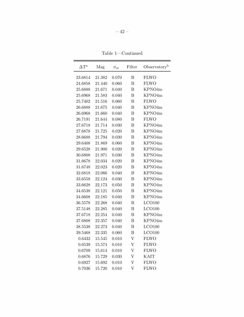
The photometric data are listed in Table 124. Much of our UBV RCIC photometry was

obtained with the F. L. Whipple Observatory (FLWO) 1.2-m telescope and the “4Shooter”

CCD mosaic (Szentgyorgyi et al., in preparation) with four thinned, back-side illuminated,

24The analysis presented here supersedes our GCN Circulars by Martini et al. (2003), Garnavich et al.

(2003d), Stanek, Martini & Garnavich (2003), Li et al. (2003a, b), Bersier et al. (2003b), and Stanek et al.

(2003b).

– 5 –

AR-coated Loral 2048 × 2048 pixel CCDs. The camera has a pixel scale of 0.335′′ pixel−1

and a field of view of roughly 11.5′ on a side for each chip. The data were taken in the 2× 2

CCD binning mode. We continuously monitored the afterglow during the first night in all

five bands, obtaining a total of 149 images. We also obtained multi-band data each night

for the next 11 nights. We then closely followed the OT in the R band with only two gaps,

when the Moon was very bright or close to the object and when the “4Shooter” was not on

the telescope25.

Extensive early UBV RI data were also obtained using an Apogee AP7 CCD camera

with the 0.76-m Katzman Automatic Imaging Telescope (KAIT; Li et al. 2000; Filippenko

et al. 2001) at Lick Observatory. The Apogee camera has a back-illuminated SITe 512×512

pixel CCD chip, which with a scale of 0.′′8 pixel−1 yields a total field of view of 6′.7 × 6′.7.

Thirteen UBV RI sets were obtained during the first night, and three sets the next night (Li

et al. 2003a).

Additional R-band images, including our earliest photometric data, were obtained using

the Magellan telescopes at Las Campanas Observatory (LCO) with the LDSS2 imaging

spectrograph (Mulchaey 2001) in its imaging mode, with a scale of 0.′′378 pixel−1. We

also obtained R-band data with the LCO Swope 1-m telescope equipped with the SITe#3

2048 × 3150 CCD camera, which with a scale of 0.′′435 pixel−1 yields a total field of view

of 14′.8 × 22′.8. Also at LCO, we obtained BV I images with the du Pont 2.5-m telescope

equipped with the TEK#5 2048 × 2048 pixel CCD camera, which with a scale of 0.′′259

pixel−1 yields a total field of view of 8′.85 × 8′.85.

In the B and R bands we obtained a significant number of images with the KPNO Mayall

4-m telescope equipped with the MOSAIC-1 wide-field camera. The prime focus Mosaic-1

camera (Muller et al. 1998) has eight CCDs covering its 36′×36′ field of view. For the

majority of the exposures, the telescope was pointed so that GRB 030329 and photometry

reference objects were all placed on the second of the eight CCDs. The images were all

processed through the reduction steps listed in version 7.01 of “The NOAO Deep Wide-Field

Survey MOSAIC Data Reductions” guide through the application of a dome flat (Jannuzi

et al. in preparation)26. The software used for the reductions is described by Valdes (2002).

All of the software is part of the MSCRED software package (v4.7), which is part of IRAF27.

25All photometry and spectroscopy presented in this paper are available through anonymous

ftp on cfa-ftp.harvard.edu, in the directory pub/kstanek/GRB030329, and through the WWW at

http://cfa-www.harvard.edu/cfa/oir/Research/GRB/.

26http://www.noao.edu/noao/noaodeep/ReductionOpt/frames.html

27IRAF is distributed by the National Optical Astronomy Observatory, which is operated by the Associa-

– 6 –

Additional late B-band data were obtained with the du Pont 2.5-m telescope. We also

obtained late B-band data with the FLWO 1.2-m telescope.

The data were reduced by several of us using different photometry packages. We used

DoPHOT (Schechter et al. 1993), DAOPHOT II (Stetson, 1987, 1992; Stetson & Harris

1988), and in some cases the image subtraction code ISIS (Alard & Lupton 1998; Alard

2000). We found excellent agreement among the various packages. Images were brought

onto a common zero point using from 10 to > 100 stars per image, depending on the filter

and depth of the image. We used several field stars measured by Henden (2003) to obtain

calibrated magnitudes.

In addition, a KAIT calibration of the GRB 030329 field was done on May 22 UT,

2003 by observing Landolt standard stars (Landolt 1992) at a large range of airmasses

under photometric conditions. Aperture photometry was performed on these standard star

frames in IRAF and then used to calibrate three local standard stars in the KAIT field of

GRB 030329. Comparison of the KAIT and the Henden calibrations shows that they are

consistent with each other (to within 0.03 mag). The KAIT data were in excellent agreement

with the overlapping FLWO data, with the largest offset of only 0.03 mag in the V band.

Such uniform data allow a great level of detail in analyzing the evolution of the OT.

In the infrared (IR), the OT was observed with the LCO Swope 1-m telescope IR camera

equipped with Rockwell NICMOS3 HgCdTe 256 × 256 pixel array with 0.′′6 pixel−1 scale,

yielding a 2′.5 × 2′.5 field of view (Persson et al. 1995). The data were obtained from 2003

April 2 to 10, using the Js and H filters. Typically, three standard stars (Persson et al.

1998) were observed each night, one each at the beginning, middle, and end of the night.

We assumed mean values of extinction appropriate at LCO: Js (0.10 mag/airmass) and H

(0.04 mag/airmass). For a comparison star near the GRB, with brightness comparable to

the OT, this resulted in photometry with a scatter lower than 0.04 mag, indicating accurate

and stable photometry for the whole run.

3. The Spectroscopic Data

Spectra of the OT associated with GRB 030329 were obtained over many nights with

the 6.5-m MMT telescope, the 1.5-m Tillinghast telescope at the F. L. Whipple Observa-

tory (FLWO), the Magellan 6.5-m Clay and Baade telescopes at LCO, the du Pont 2.5-m

tion of Universities for Research in Astronomy, Inc., under cooperative agreement with the National Science

Foundation.

– 7 –

telescope at LCO, the Shane 3-m telescope at Lick Observatory, and the Keck I and II 10-m

telescopes28. The majority of the data discussed herein are from the MMT. The spectro-

graphs used were the Blue Channel (Schmidt et al. 1989) at MMT, FAST (Fabricant et

al. 1998) at FLWO, LDSS2 (Mulchaey 2001) with Clay, the Boller & Chivens (Phillips et

al. 2002) with Baade, the WFCCD (Weymann et al. 1999) with du Pont, the Kast Dou-

ble Spectrograph (Miller & Stone 1993) at Lick, LRIS (Oke et al. 1995) with Keck I, and

ESI (Sheinis et al. 2002) with Keck II. Standard CCD processing and spectrum extraction

were accomplished with IRAF. Except for the April 24 ESI data, all spectra were optimally

extracted (Horne 1986). The wavelength scale was established with low-order polynomial

fits to calibration lamp spectra taken near the times of the OT exposures. Small-scale ad-

justments derived from night-sky lines in the OT frames were also applied. We employed

our own routines in IDL to flux calibrate the spectra; spectrophotometric standards, along

with other observational details, are listed in Table 2. We attempted to remove telluric lines

using the well-exposed continua of the spectrophotometric standards (Wade & Horne 1988;

Matheson et al. 2000).

The spectra were in general taken at or near the parallactic angle (Filippenko 1982)

and at low airmass (with the obvious exception of observations from LCO). The relative

fluxes are thus accurate to ∼ 5% over the entire wavelength range. The Blue Channel,

LDSS2, and Boller & Chivens spectrographs suffer from second-order contamination with

the gratings used for these observations. Through careful cross-calibration with standard

stars of different colors (and order-sorting filters with the Boller & Chivens), we believe that

we have minimized the effects of the second-order light. For the few nights at the MMT

when a broad range of standard stars of different colors was not available, we used the

closest match from either the preceding or following night. Comparison with broad-band

photometry indicates that the overall shape of the spectra is correct.

4. Early Photometry and Spectroscopy: Days 1-12

The transition between the afterglow and the supernova was gradual, so we define our

“early” data based on our observations. We obtained spectroscopic data each of the 12

nights between March 30 and April 10. For each of these nights, we also obtained multi-

band photometric data.

28The analysis presented here supersedes our GCN and IAU Circulars by Martini et al. (2003), Caldwell

et al. (2003), Matheson et al. (2003a), Garnavich et al. (2003b), Matheson et al. (2003b), Garnavich et al.

(2003c), and Chornock et al. (2003).

– 8 –

4.1. Early Photometry

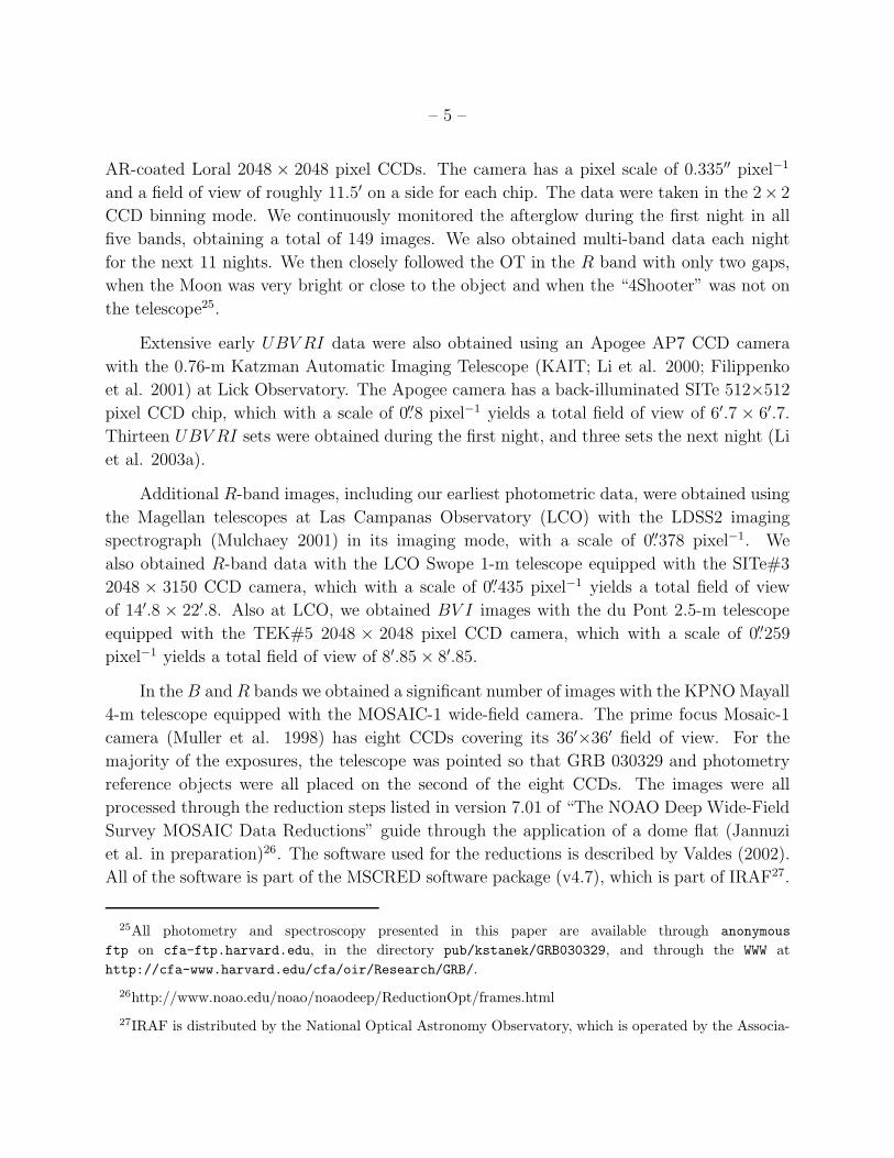
We plot our GRB 030329 UBV RIJH light curves in Figure 1. Within the first 24 hours,

the light curve of the afterglow consisted of a broken power law typical of many well-observed

bursts (Garnavich et al. 2003d). But the optical afterglow exhibited unusual behavior over

the following week that has been analyzed in numerous GCNs (e.g., Li et al. 2003b, c). As it

is clear that the afterglow cannot be well described with any semblance of a smooth function

usually fitted to describe the OT evolution, we present and discuss here only our data.

Such uniform data allow a great level of detail and confidence in analyzing the evolution of

the GRB, including color changes, not usually possible when using non-homogeneous data

compiled from the GCNs and the literature.

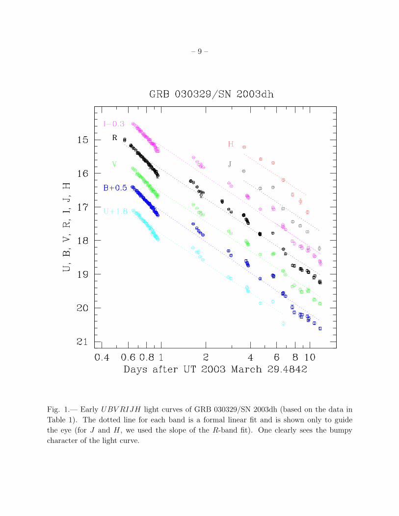
This is another clear example of an OT changing color as it fades. A color change was

also seen in the OT of GRB 021004 (Matheson et al. 2003c; Bersier et al. 2003a). The color

curves of the OT of GRB 030329 are plotted in Figure 2, in which the color changes are

more readily apparent (see also Zeh, Klose, & Greiner 2003). These changes are discussed in

more detail below when we describe the evolution of the spectral energy distribution (SED).

GRB 030329 is located at Galactic coordinates l = 216.9867, b = 60.6997. To remove

the effects of the Galactic interstellar extinction we used the reddening map of Schlegel,

Finkbeiner, & Davis (1998) which yields E(B − V ) = 0.025 mag. This corresponds to

expected values of Galactic extinction ranging from AH = 0.014 to AU = 0.137 mag, using

the extinction corrections of Cardelli, Clayton, & Mathis (1989) and O’Donnell (1994) as

prescribed in Schlegel et al. (1998).

We synthesized the UBV RI spectrum for the first seven nights and BV RI spectra for

later nights from our data by using our best, most closely spaced measurements for all the

nights (Figure 3). We converted the magnitudes to fluxes using the effective frequencies and

normalizations of Fukugita et al. (1995). These conversions are accurate to better than 4%,

so to account for the calibration errors we added a 4% error in quadrature to the statistical

error in each flux measurement.

There are several evolutionary stages to be noticed in Figure 3. First, the SED gradually

evolves between the first and the third night (see the dotted line in Figure 3), with the

spectrum becoming steeper (redder). The spectral index, corrected for Galactic reddening

of E(B − V ) = 0.025 mag, changes from −0.71 the first night, through −0.89 the second

night, to −0.97 the third night. Our early shallower slope agrees well with the −0.66 slope

measured by Burenin et al. (2003) in their earlier data taken 6 − 11 hours after the burst.

Our data are also consistent with the dereddened spectral slope of −0.85 found using SDSS

photometry coinciding with our second night data (Lee et al. 2003). Then, at ∆T = 4.65 days

– 9 –

Fig. 1.— Early UBV RIJH light curves of GRB 030329/SN 2003dh (based on the data in

Table 1). The dotted line for each band is a formal linear fit and is shown only to guide

the eye (for J and H , we used the slope of the R-band fit). One clearly sees the bumpy

character of the light curve.

– 10 –

Fig. 2.— Early color evolution of the OT. Fiducial levels (dotted lines) represent the value

of the first point for each color.

– 11 –

Fig. 3.— Spectral energy distribution (SED) of the optical afterglow of GRB 030329 at

various times (indicated on the right side of each SED for nights 1-7 and on the left side for

nights 8-12). We superimposed an MMT spectrum obtained nearly simultaneously with our

photometry at ∆T = 5.64 days (our fiducial spectrum). The SED from ∆T = 0.65 days is

shown (dotted line) on top of the SED from ∆T = 2.86 days. The SED from ∆T = 5.64

days is shown (dash-dotted line) on top of the SED from ∆T = 9.77 days. For clarity, SEDs

from ∆T = 5.64, 9.77, 10.67, and 11.82 days were multiplied by 0.8.

– 12 –

(where ∆T is the time since the GRB), the red part of the SED (V RI) remains unchanged,

while the blue part of the SED (UB) is clearly depressed by about 0.1 mag. On the following

epoch, ∆T = 5.64 days, the SED “recovers” and resembles closely the SEDs from nights

3-4. After ∆T = 6.66 days, as discussed below, the supernova component starts to emerge

quickly and the colors and SEDs undergo dramatic evolution: while nearly unchanged in

V − R, the transient becomes more red in B − V and strongly bluer in R − I, R − J , and

R−H . Similar color changes at early times (without UJH) were discussed in GCN Circulars

by Bersier et al. (2003b) and Henden et al. (2003). This peculiar color change is because

the supernova flux peaks around 6000 A, raising V and R nearly equally while the bands

redward and blueward slope up toward the peak.

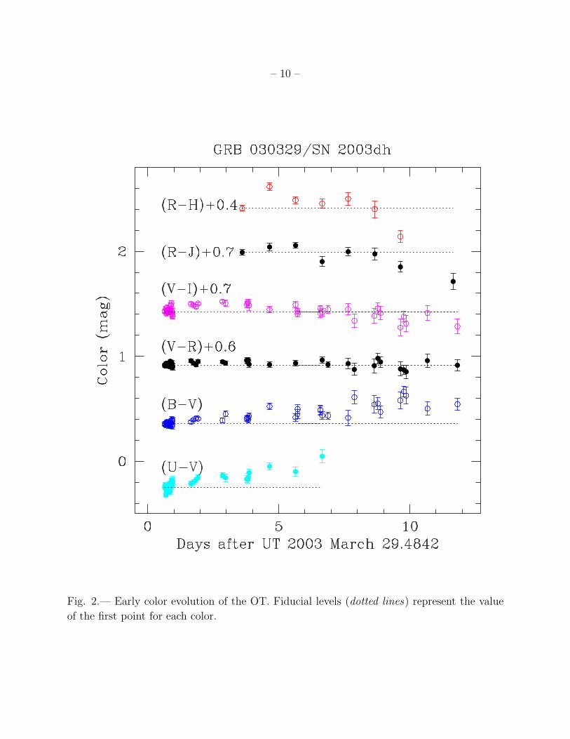
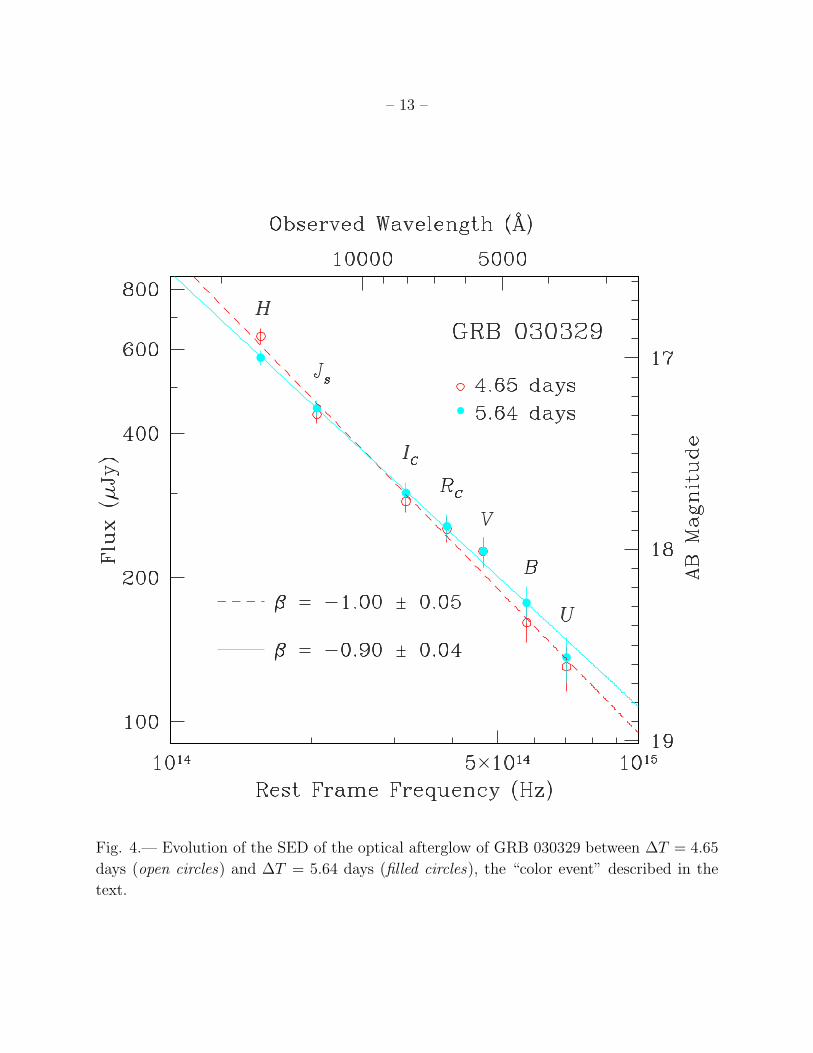
The “color event” of ∆T = 4.65 days is also present in the near-IR data, as can be seen

in Figure 2. To highlight this color change, we show in Figure 4 the evolution of the SED of

the optical afterglow of GRB 030329 between ∆T = 4.65 days and ∆T = 5.64 days.

4.2. Early Spectroscopy

The brightness of the OT allowed us to observe the OT each of the 12 nights between

March 30 and April 10 UT, mostly with the MMT 6.5-m, but also with the Magellan 6.5-m,

Lick Observatory 3-m, LCO du Pont 2.5-m, and FLWO 1.5-m telescopes. This provided a

unique opportunity to look for spectroscopic evolution over many nights. The early spectra

of the OT of GRB 030329 (top of Figure 5) consist of a power-law continuum typical of GRB

afterglows, with narrow emission features identifiable as Hα, [O III] λλ4959, 5007, Hβ, and

[O II] λ3727 at z = 0.1685 (Greiner et al. 2003; Caldwell et al. 2003) probably from H II

regions in the host galaxy. Assuming a Lambda cosmology with H0 = 70 km s−1 Mpc−1,

Ωm = 0.3, and ΩΛ = 0.7, this redshift corresponds to a luminosity distance of 810 Mpc.

Beginning at ∆T = 7.67 days, our spectra deviated from the pure power-law continuum.

Broad peaks in flux, characteristic of a supernova, appeared. The broad bumps are seen at

approximately 5000 A and 4200 A (rest frame). At that time, the spectrum of GRB 030329

looked similar to that of the peculiar Type Ic SN 1998bw a week before maximum light

(Patat et al. 2001) superposed on a typical afterglow continuum. Over the next few days the

SN features became more prominent as the afterglow faded and the SN brightened toward

maximum.

– 13 –

Fig. 4.— Evolution of the SED of the optical afterglow of GRB 030329 between ∆T = 4.65

days (open circles) and ∆T = 5.64 days (filled circles), the “color event” described in the

text.

– 14 –

4000 5000 6000 7000 8000 9000Observed Wavelength (Å)

24

22

20

18

16

−2.

5log

(f λ)

+ C

onst

ant

0.75

1.73

2.66

3.70

4.66

5.80

6.66

7.67

8.78

9.67

10.68

11.66

Fig. 5.— Evolution of the GRB 030329/SN 2003dh spectrum, from March 30.23 UT (0.75

days after the burst), to April 10.14 UT (11.66 days after the burst). The early spectra

consist of a power-law continuum with narrow emission lines originating from H II regions

in the host galaxy at z = 0.1685. Spectra taken after ∆T = 6.66 days show the development

of broad peaks characteristic of a supernova. In some spectra, regions of bad fringing or

low signal-to-noise ratio have been removed for clarity. Spectra from ∆T = 3.70, 10.68, and

11.66 days have been rebinned to improve the signal-to-noise ratio. Note that not all spectra

listed in Table 2 are presented in this figure.

– 15 –

5. Later Photometry and Spectroscopy: Days 13-61

5.1. Later Photometry

We continued observing the OT in the R band using mostly the FLWO 1.2-m telescope,

and also obtaining some data with the KPNO 4-m and the LCO Swope 1-m telescopes. In

the B band, we obtained most of the later data with the KPNO 4-m, and also some data with

the du Pont 2.5-m and the FLWO 1.2-m telescopes. The two gaps in the R-band coverage

correspond to the Moon being bright or near the position of the OT, and also when the CCD

camera was not mounted. The results are shown in Figure 6.

There are several interesting features to be seen in Figure 6. Coinciding with the first

detection of the supernova in the spectra, both R and B light curves start to decay more

slowly (this can be also seen in Figure 1). In addition, the (B − R) color undergoes a

dramatic change at later times, as can be seen in the lower panel of Figure 6. Both of these

characteristics result from the supernova component, redder in (B −R) color than the GRB

afterglow, strongly contributing to the total light of the OT starting at ∆T = 7.67 days.

The strong (B − R) color change indicates that at later times the supernova component

dominates the total light, as will be discussed in more detail later in the paper.

Another striking feature is the “Jitter Episode” (Stanek, Latham, & Everett 2003;

Stanek et al. 2003c; Ibrahimov et al. 2003) in the late R-band light curve observed between

51.75 and 60.7 days after the burst. The light curve is seen to vary on timescales of ∼ 2 days

by > 0.3 mag, such as when the OT brightens from R = 21.70 ± 0.11 mag at ∆T = 52.71

days to R = 21.31± 0.09 mag at ∆T = 54.69 days, only to fade to R = 21.61± 0.06 mag at

∆T = 57.72 days.

We should stress that these data were obtained with exactly the same instrumentation

and reduced with the same software and in the same manner as our earlier, much smoother

data (see Figure 6). This “Jitter Episode” is unusual when compared to the whole data set

and we strongly believe that it is real. We will discuss it in more detail later in the paper.

5.2. Later Spectroscopy

Later spectra obtained on April 24.28, May 2.05, May 4.01, and May 24.38 continue

to show the characteristics of a supernova. As the power-law continuum of the GRB after-

glow fades, the supernova spectrum rises, becoming the dominant component of the overall

spectrum (Figure 7).

– 16 –

Fig. 6.— Upper panel: B-band (open circles) and R-band (filled circles) photometry at later

times, with the last R-band epoch at ∆T = 60.7 days after the burst. The first two arrows

correspond to the first time when the supernova signature could be seen in the spectra and

the last spectrum in the continuous series. The remaining arrows correspond to our spectra

taken after ∆T = 12.0 days. Lower panel: B − R color evolution in later times. The solid

line indicates the color expected for an afterglow with a fixed power-law spectrum plus a

supernova like SN 1998bw K-corrected to the redshift of GRB 030329. Contamination from

the host galaxy may contribute to the B-band light at late times.

– 17 –


26

24

22

20

−2.

5log

(f λ)

+ C

onst

ant

25.80

33.57

35.53

55.90

Fig. 7.— Evolution of the GRB 030329/SN 2003dh spectrum, from April 24.28 UT (25.8

days after the burst), to May 24.38 (55.9 days after the burst). The power-law contribu-

tion decreases and the spectra become more red as the SN component begins to dominate,

although the upturn at blue wavelengths may still be the power law. The broad features

of a supernova are readily apparent, and the overall spectrum continues to resemble that of

SN 1998bw several days after maximum. The ∆T = 25.8 days spectrum is a combination

of the ∆T = 25.71 days MMT spectrum and the ∆T = 25.89 days ESI spectrum. The dip

near 5600 A in the ∆T = 55.90 days spectrum is due to the dichroic used in LRIS, and is

not intrinsic to the OT.

– 18 –

6. Analysis

6.1. Properties of the Host

The low redshift of this burst meant that the rest-frame optical spectrum of the host

galaxy could be obtained, thus allowing the use of well-tested techniques for measuring the

metallicity, reddening, and star-formation rate of the host. The MMT spectra from the

nights of 2003 Apr 4, 5, 7, and 8 UT were averaged together and a low-order fit to the

continuum was subtracted, since the SN was apparent in the averaged spectrum. At a later

date when the optical transient has completely faded, it will be valuable to get a spectrum

showing the absorption-line component, but the present spectrum is suitable for studying

the emission-line component. HST images and spectra (Fruchter et al. 2003) show the host

to extend to about 0.5′′, so most of the light of the host galaxy should be contained within

the MMT slit used even though the GRB was off center. The Hα flux measured should thus

refer to the entire galaxy, at least for those nights where the seeing was good.

Overall, the emission-line spectrum shows strong forbidden oxygen lines and hydrogen

Balmer lines, but no detection of the [N II] λλ6548, 6584 lines, with line ratios indicative

of low-metallicity gas photoionized by stars. Table 3 lists the observed ratios, measured

using the IRAF “splot” routine. We first estimate the reddening using the Hα/Hβ line-

intensity ratio as a measure of the Balmer decrement, assuming Case B recombination (e.g.,

Osterbrock 1989) and the Whitford extinction law. The redshifted Hα line is affected by

telluric absorption, which may have lead to errors in the Hα/Hβ ratio, but the dominant

source of error in the line ratios is simply photon counting. The reddening implied by the

difference between the observed ratio and the theoretical value is in the range E(B − V ) =

0.05 - 0.11 mag. If the Galactic foreground reddening is E(B − V ) = 0.025 mag (Schlegel et

al. 1998), then the reddening intrinsic to the host is in the range 0.03 to 0.09 mag.

To estimate the oxygen abundance in the host, we use the R23 method that employs the

ratios of [O III]/[O II], [N II]/[O II], and [O II]+[O III]/Hβ (Pagel 1986; Kewley & Dopita

2002). Using a reddening of 0.05 mag to correct the line ratios, and the parameterizations

found in Kewley & Dopita, we derive an ionization parameter q = 2 × 107 cm s−1, which

then leads to an oxygen abundance of log(O/H)+12 = 8.5, or about 0.5 Z⊙. The lack of

detectable [N II] is consistent with this moderate metallicity.

The Hα flux was measured from the spectrum of 2003 April 8, and when corrected for

reddening, gives an Hα luminosity of L(Hα) = 6.6 × 1040 erg s−1, for a distance of 810

Mpc. This corresponds to a current star formation rate of 7.9× 10−42 L(Hα) = 0.5 M⊙ yr−1

(Kennicutt 1998). This would be a modest star formation rate in a large galaxy, but the

host of GRB 030329 is probably a dwarf. Fruchter et al. (2003) estimate the magnitude of

– 19 –

the host to be V = 22.7, meaning MV = −16.9 mag, which is similar to the luminosity of the

SMC. The moderate metallicity we have calculated is in accord with the galaxy luminosity, in

this case corresponding well with that of the LMC, which has a metallicity of log(O/H)+12

= 8.4 (Russell & Dopita 1990).

Star formation rates in dwarfs can vary widely. Hunter, Hawley, & Gallagher (1993)

report a range of rates from 0.001 to 3 M⊙ yr−1, the latter limit referring to starburst dwarfs

such as NGC 1569. The mean value is around 0.03 M⊙ yr−1. A useful comparison of star

formation ability in local dwarf galaxies can then be made by calculating the birthrate, the

ratio of the current star formation rate to the average past rate. We estimate this quantity

simply by normalizing the current rate to the galaxy blue luminosity divided by an age of

12 Gyr, and assuming M/L = 3. For the host of GRB 030329, the birthrate is about 5 M⊙

yr−1. That can be compared to the SMC value of 0.3 M⊙ yr−1, and the value of 2 M⊙ yr−1

for the starburst galaxy NGC 1569 (derived from data in Hunter et al. 1993 and Kennicutt

& Hodge 1986). One is driven to the conclusion that the GRB 030329 host is also a starburst

dwarf galaxy.

The more massive hosts of other GRBs also show large star formation rates, particularly

when measured via radio or sub-mm techniques. Berger et al. (2003) calculate rates of 100-

500 M⊙ yr−1 in bolometrically luminous hosts (L > 1012 L⊙). However, the rates derived

from an optical emission line ([O II] λ3727) for other GRB hosts are much lower, 1− 10 M⊙

yr−1 (Djorgovski et al. 2001). The discrepancy in rates is not yet understood, particularly

since the extinction measured in the optical for the Djorgovski hosts is low, as we have found

here. Sub-mm observations of the host of GRB 030329 would be interesting in this regard.

6.2. Extinction Toward the GRB in the Host

We used our UBV RCICJsH photometry from ∆T = 5.64 days after the burst to inves-

tigate whether there is any evidence for extinction in the host galaxy along the line of sight

to GRB 030329/SN 2003dh. The optical and infrared magnitudes were converted to flux

densities based on the AB corrections given in Fukugita et al. (1995) and Megessier (1995).

Each data point was corrected for a small Galactic reddening of E(B − V ) = 0.025 ± 0.020

mag (Schlegel et al. 1998). No corrections were applied for any reddening that may be

present in the host galaxy or in intergalactic space between us and the host.

The spectral energy distribution was fit by fν(ν) ∝ νβ × 10−0.4A(ν), where fν(ν) is the

flux density at frequency ν, β is the intrinsic spectral index, and A(ν) is the extragalactic

extinction along the line of sight to the burst. The dependence of A(ν) on ν has been

– 20 –

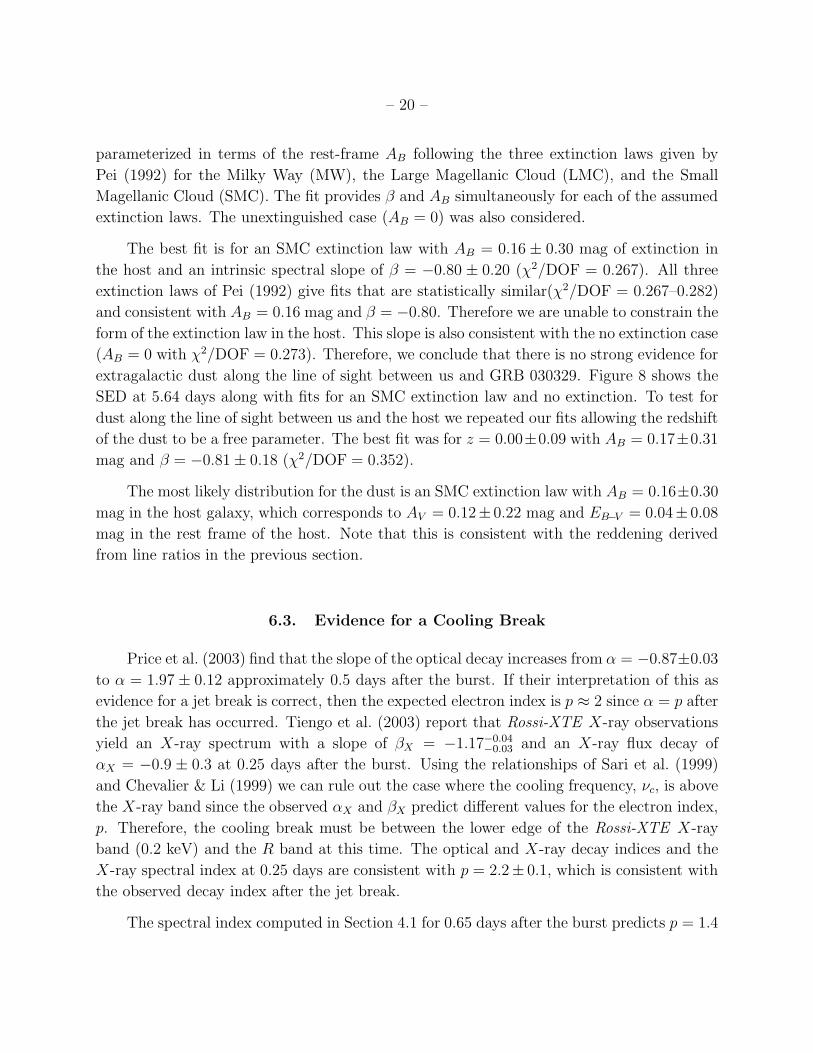
parameterized in terms of the rest-frame AB following the three extinction laws given by

Pei (1992) for the Milky Way (MW), the Large Magellanic Cloud (LMC), and the Small

Magellanic Cloud (SMC). The fit provides β and AB simultaneously for each of the assumed

extinction laws. The unextinguished case (AB = 0) was also considered.

The best fit is for an SMC extinction law with AB = 0.16 ± 0.30 mag of extinction in

the host and an intrinsic spectral slope of β = −0.80 ± 0.20 (χ2/DOF = 0.267). All three

extinction laws of Pei (1992) give fits that are statistically similar(χ2/DOF = 0.267–0.282)

and consistent with AB = 0.16 mag and β = −0.80. Therefore we are unable to constrain the

form of the extinction law in the host. This slope is also consistent with the no extinction case

(AB = 0 with χ2/DOF = 0.273). Therefore, we conclude that there is no strong evidence for

extragalactic dust along the line of sight between us and GRB 030329. Figure 8 shows the

SED at 5.64 days along with fits for an SMC extinction law and no extinction. To test for

dust along the line of sight between us and the host we repeated our fits allowing the redshift

of the dust to be a free parameter. The best fit was for z = 0.00±0.09 with AB = 0.17±0.31

mag and β = −0.81 ± 0.18 (χ2/DOF = 0.352).

The most likely distribution for the dust is an SMC extinction law with AB = 0.16±0.30

mag in the host galaxy, which corresponds to AV = 0.12± 0.22 mag and EB−V = 0.04± 0.08

mag in the rest frame of the host. Note that this is consistent with the reddening derived

from line ratios in the previous section.

6.3. Evidence for a Cooling Break

Price et al. (2003) find that the slope of the optical decay increases from α = −0.87±0.03

to α = 1.97 ± 0.12 approximately 0.5 days after the burst. If their interpretation of this as

evidence for a jet break is correct, then the expected electron index is p ≈ 2 since α = p after

the jet break has occurred. Tiengo et al. (2003) report that Rossi-XTE X-ray observations

yield an X-ray spectrum with a slope of βX = −1.17−0.04−0.03 and an X-ray flux decay of

αX = −0.9 ± 0.3 at 0.25 days after the burst. Using the relationships of Sari et al. (1999)

and Chevalier & Li (1999) we can rule out the case where the cooling frequency, νc, is above

the X-ray band since the observed αX and βX predict different values for the electron index,

p. Therefore, the cooling break must be between the lower edge of the Rossi-XTE X-ray

band (0.2 keV) and the R band at this time. The optical and X-ray decay indices and the

X-ray spectral index at 0.25 days are consistent with p = 2.2± 0.1, which is consistent with

the observed decay index after the jet break.

The spectral index computed in Section 4.1 for 0.65 days after the burst predicts p = 1.4

– 21 –

Fig. 8.— Spectral energy distribution of the optical afterglow of GRB 030329/SN 2003dh at

∆T = 5.64 days after the burst. The filled circles represent observed photometry corrected

for extinction in the Milky Way and shifted to the rest frame of the host galaxy. The lines

represent the best-fitting spectral energy distribution, assuming an SMC extinction law (solid

line) or no extinction (dashed line). If we assume that the unextinguished spectrum follows

fν(ν) ∝ νβ then the best fit has β0 = −0.80 ± 0.20 and AB = 0.16 ± 0.30 mag.

– 22 –

if the cooling break frequency is below the optical and p = 2.4 if it is above the optical. Values

for the electron index of less than two represent infinite energy in the electrons. This strongly

suggests that νc > νR at this time. However, at 1.65 ≤ ∆T ≤ 5.64 days the optical spectral

slopes (see Section 4.1) are consistent with νc < νR and p ≈ 2. The case where νc > νR at

these times implies p ≈ 3, which is inconsistent with the value of the electron index that was

derived for ∆T = 0.25 days. Tiengo et al. (2003) used XMM-Newton X-ray observations to

find βX = −0.92+0.26−0.15 at 37 days and β = −1.1+0.4

−0.2 at 61 days. Both of these are consistent

with p ≈ 2 and νc < νR. Therefore we believe that the cooling break passed through the

optical, moving toward radio frequencies, between 0.65 and 1.65 days after the burst. A

cooling frequency that decreases with time is the hallmark of a homogeneous interstellar

medium. However, there may be local inhomogeneities on scales that are small compared to

the size of the fireball.

At X-ray frequencies interstellar absorption does not significantly affect the slope of the

spectrum, so the observed slope is a good approximation of the actual slope. Combining all

of the βX values from Tiengo et al. (2003) yields p = 2.2±0.1. This predicts that the optical

spectrum has β = −1.10± 0.05 at ∆T = 5.64 days, which is close to the observed spectrum.

This agreement strengthens our conclusion in Section 6.2 that there is no strong evidence

for dust in the host galaxy along the line of sight to the burst.

6.4. Separating the GRB from the Supernova

To explore the nature of the supernova underlying the OT, we modeled the spectrum

as the sum of a power-law continuum and a peculiar Type Ic SN. Specifically, we chose for

comparison SN 1998bw (Patat et al. 2001), SN 1997ef (Iwamoto et al. 2000), and SN 2002ap

(using our own as yet unpublished spectra, but see, e.g., Kinugasa et al. 2002; Foley et

al. 2003). We had 62 spectra of these three SNe, spanning the epochs of seven days before

maximum to several weeks past. For the power-law continuum, we chose to use one of our

early spectra to represent the afterglow of the GRB. The spectrum at time ∆T = 5.80

days was of high signal-to-noise ratio (S/N), and suffers from little fringing at the red end.

Therefore, we smoothed this spectrum to provide the fiducial power-law continuum of the

OT for our model. Other choices for the continuum did not affect our results significantly.

To find the best match with a supernova spectrum, we compared each spectrum of

the afterglow with the sum of the fiducial continuum and a spectrum of one of the SNe in

the sample, both scaled in flux to match the OT spectra. We performed a least-squares fit,

allowing the fraction of continuum and SN to vary, finding the best combination of continuum

and SN for each of the SN spectra. The minimum least-squares deviation within this set was

– 23 –

then taken as the best SN match for that epoch of OT observation. The results of the fits

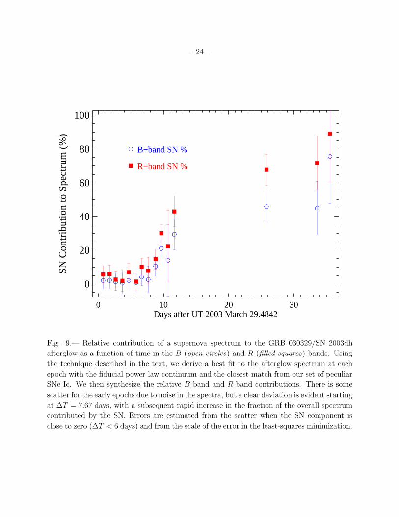
for the spectra we modeled are listed in Table 4. Figure 9 shows the relative contribution to

the OT spectrum by the underlying SN in the B and R bands as a function of ∆T .

Within the uncertainties of our fit, the SN fraction is consistent with zero for the first

few days after the GRB. At ∆T = 7.67 days, the SN begins to appear in the spectrum,

without strong evidence for a supernova component before this. Hjorth et al. (2003) report

evidence for the SN spectrum in their April 3 UT data (∆T ≈ 4 days), but we do not see

any sign of a SN component at this time. There is a color change near ∆T ≈ 5 days as noted

above (see also Figure 3), but we attribute it to the afterglow. Our decomposition of the

photometry into SN and afterglow components (see below) indicates that, at most, the SN

would have contributed only a few percent of the total light at this point, making it difficult

to identify indisputable features.

Note that when the fit indicates the presence of a supernova, the best match is almost

always SN 1998bw. The only exceptions to this are from nights when the spectrum of the

OT are extremely noisy, implying that less weight should be given to those results. The

least-squares deviation for the spectra that do not match SN 1998bw is also much larger (see

Table 4).

Our best spectrum (i.e., with the highest S/N) from this time when the SN features

begin to appear is at ∆T = 9.67 days. In Figure 10, our best fit of 74% continuum and

26% SN 1998bw (at day −6 relative to SN B-band maximum) is plotted over the observed

spectrum from this epoch. The next-best fit is SN 1998bw at day −7. Using a different early

epoch to define the reference continuum does not alter these results significantly. It causes

slight changes in the relative percentages, but the same SN spectrum still produces the best

fit, albeit with a larger least-squares deviation.

The SN fraction contributing to the total spectrum increases steadily with time. By

∆T = 25.8 days, the SN fraction is ∼ 61%, with the best-fit SN being SN 1998bw at day +6

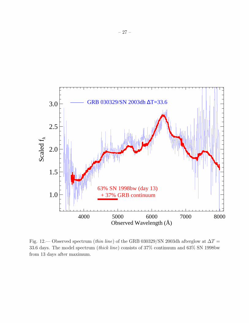
(Figure 11). The SN percentage at ∆T = 33.6 days is still about 63%, but the best match is

now SN 1998bw at day +13 (Figure 12). The rest-frame time difference between ∆T = 9.67

days and ∆T = 25.8 days is 13.8 days (z = 0.1685). For the best-fit SN spectra from those

epochs, SN 1998bw at day −6 and SN 1998bw at day +6 respectively, the time difference

is 12 days. The rest-frame time difference between ∆T = 25.8 days and ∆T = 33.6 days is

6.7 days, with a time difference between the best-fit spectra for those epochs of 7 days. The

spectral evolution determined from these fits indicates that SN 2003dh follows SN 1998bw

closely, and it is not as similar to SN 1997ef or SN 2002ap. The analysis by Kawabata et

al. (2003) of their May 10 spectrum gives a phase for the spectrum of SN 2003dh that is

consistent with our dates, although they do consider SN 1997ef as a viable alternative to

– 24 –

0 10 20 30Days after UT 2003 March 29.4842

0

20

40

60

80

100

SN

Con

trib

utio

n to

Spe

ctru

m (

%)

B−band SN %

R−band SN %

Fig. 9.— Relative contribution of a supernova spectrum to the GRB 030329/SN 2003dh

afterglow as a function of time in the B (open circles) and R (filled squares) bands. Using

the technique described in the text, we derive a best fit to the afterglow spectrum at each

epoch with the fiducial power-law continuum and the closest match from our set of peculiar

SNe Ic. We then synthesize the relative B-band and R-band contributions. There is some

scatter for the early epochs due to noise in the spectra, but a clear deviation is evident starting

at ∆T = 7.67 days, with a subsequent rapid increase in the fraction of the overall spectrum

contributed by the SN. Errors are estimated from the scatter when the SN component is

close to zero (∆T < 6 days) and from the scale of the error in the least-squares minimization.

– 25 –

4000 5000 6000 7000 8000Observed Wavelength (Å)

1.0

1.5

2.0

2.5

3.0

Sca

led

f λ

GRB 030329/SN 2003dh ∆T=9.7

26% SN 1998bw (day −6)

+ 74% GRB continuum

Fig. 10.— Observed spectrum (thin line) of the GRB 030329/SN 2003dh afterglow at ∆T =

9.67 days. The model spectrum (thick line) consists of 74% continuum and 26% SN 1998bw

from 6 days before maximum. No other peculiar SN Ic spectrum provided as good a fit.

– 26 –


0.5

1.0

1.5

2.0

2.5

Sca

led

f λ

GRB 030329/SN 2003dh

∆T=25.8

61% SN 1998bw (day +6)

+ 39% GRB continuum



from 6 days after maximum.

– 27 –

4000 5000 6000 7000 8000Observed Wavelength (Å)

1.0

1.5

2.0

2.5

3.0

Sca

led

f λ

GRB 030329/SN 2003dh ∆T=33.6

63% SN 1998bw (day 13)+ 37% GRB continuum



from 13 days after maximum.

– 28 –

SN 1998bw as a match for the SN component in the afterglow.

Once the spectrum of the SN has been separated from the power-law continuum of the

afterglow, one can consider the nature of SN 2003dh itself. The spectrum does not show

any sign of broad hydrogen lines, eliminating the Type II classification, nor is there the deep

Si II λ6355 (usually blueshifted to ∼6150 A) feature that is the hallmark of Type Ia SNe.

The optical helium line absorptions that indicate SNe of Type Ib are not apparent either.

This leads to a classification of SN 2003dh as a Type Ic (see Filippenko 1997 for a review

of supernova classification). Given the striking correspondence with the Type Ic SN 1998bw

shown above, this is a natural classification for SN 2003dh.

The spectra of SN 1998bw (and other highly energetic SNe) are not simple to interpret.

The high expansion velocities result in many overlapping lines so that identification of specific

line features is problematic for the early phases of spectral evolution (see, e.g., Iwamoto et

al. 1998; Stathakis et al. 2000; Nakamura et al. 2001; Patat et al. 2001). This includes

spectra up to two weeks after maximum, approximately the same epochs covered by our

spectra of SN 2003dh. In fact, as Iwamoto et al. (1998) showed, the spectra at these phases

do not show line features. The peaks in the spectra are due to gaps in opacity, not individual

spectral lines. Detailed modeling of the spectra can reveal some aspects of the composition of

the ejecta (e.g., Nakamura et al. 2001). Such a model is beyond the scope of this paper, but

the spectra discussed herein and the spectrum of Kawabata et al. (2003) are being analyzed

for a future paper (Mazzali et al., in preparation).

If the ∆T = 9.67 days spectrum for the afterglow does match SN 1998bw at day −6,

then limits can be placed on the timing of the supernova explosion relative to the GRB. The

rest-frame time for ∆T = 9.67 days is 8.2 days, implying that the time of the GRB would

correspond to ∼14 days before maximum for the SN. The rise times of SNe Ic are not well

determined, especially for the small subset of peculiar ones. Stritzinger et al. (2002) found

the rise time of the Type Ib/c SN 1999ex was ∼18 days (in the B band), while Richmond

et al. (1996) reported a rise time of ∼12 days (in the V band) for the Type Ic SN 1994I.

A rise time of ∼14 days for SN 2003dh is certainly a reasonable number. It also makes it

extremely unlikely that the SN exploded significantly earlier or later than the time of the

GRB, most likely within ±2 days of the GRB itself.

The totality of data contained in this paper allows us to attempt to decompose the light

curve of the OT into the supernova and the afterglow (power-law) component. From the

spectral decomposition procedure described above, we have the fraction of light in the BR-

bands for both components at various times, assuming that the spectrum of the afterglow

did not evolve since ∆T = 5.64 days. As we find that the spectral evolution is remarkably

close to that of SN 1998bw, we model the R-band supernova component with the V -band

– 29 –

light curve of SN 1998bw (Galama et al. 1998a, b) stretched by (1+ z) = 1.1685 and shifted

in magnitude to obtain a good fit. The afterglow component is fit by using the early points

starting at ∆T = 5.64 days with late points obtained via the spectral decomposition. This

can be done in both in the B and in the R-band and leads to consistent results, indicating

that our assumption of the afterglow not evolving in color at later times is indeed valid.

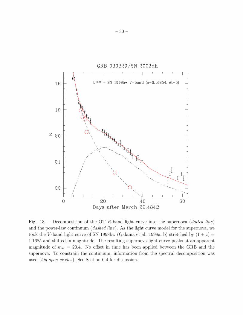
The result of the decomposition of the OT R-band light curve into the supernova and

the power-law continuum is shown in Figure 13. The overall fit is remarkably good, given

the assumptions (such as using the stretched V -band light curve of SN 1998bw as a proxy for

the SN 2003dh R-band light curve). No time offset between the supernova and the GRB was

applied, and given how good the fit is, we decided not to explore time offset as an additional

parameter. Introducing such an additional parameter would most likely result in a somewhat

better fit (indeed, we find that to be the case for δt ≈ −2 days), but this could easily be

an artifact with no physical significance, purely due to small differences between SN 1998bw

and SN 2003dh. At this point the assumption that the GRB and the SN happened at the

same time seems most natural.

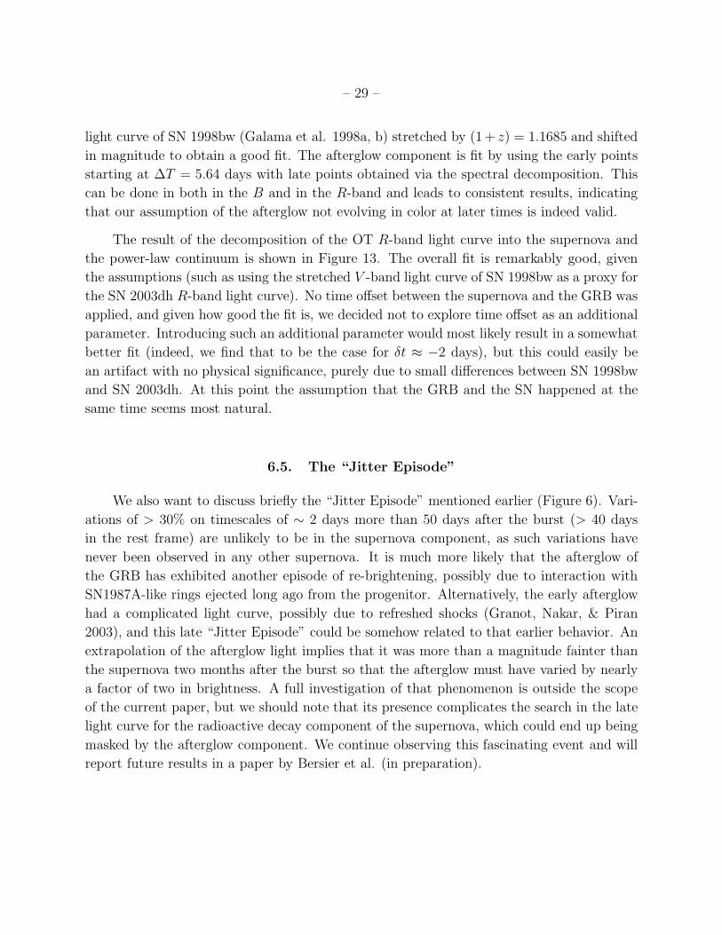
6.5. The “Jitter Episode”

We also want to discuss briefly the “Jitter Episode” mentioned earlier (Figure 6). Vari-

ations of > 30% on timescales of ∼ 2 days more than 50 days after the burst (> 40 days

in the rest frame) are unlikely to be in the supernova component, as such variations have

never been observed in any other supernova. It is much more likely that the afterglow of

the GRB has exhibited another episode of re-brightening, possibly due to interaction with

SN1987A-like rings ejected long ago from the progenitor. Alternatively, the early afterglow

had a complicated light curve, possibly due to refreshed shocks (Granot, Nakar, & Piran

2003), and this late “Jitter Episode” could be somehow related to that earlier behavior. An

extrapolation of the afterglow light implies that it was more than a magnitude fainter than

the supernova two months after the burst so that the afterglow must have varied by nearly

a factor of two in brightness. A full investigation of that phenomenon is outside the scope

of the current paper, but we should note that its presence complicates the search in the late

light curve for the radioactive decay component of the supernova, which could end up being

masked by the afterglow component. We continue observing this fascinating event and will

report future results in a paper by Bersier et al. (in preparation).

– 30 –

Fig. 13.— Decomposition of the OT R-band light curve into the supernova (dotted line)

and the power-law continuum (dashed line). As the light curve model for the supernova, we

took the V -band light curve of SN 1998bw (Galama et al. 1998a, b) stretched by (1 + z) =

1.1685 and shifted in magnitude. The resulting supernova light curve peaks at an apparent

magnitude of mR = 20.4. No offset in time has been applied between the GRB and the

supernova. To constrain the continuum, information from the spectral decomposition was

used (big open circles). See Section 6.4 for discussion.

– 31 –

7. Summary

We have presented optical and infrared photometry and optical spectroscopy of

GRB 030329/SN 2003dh covering the first two months of its evolution. The early photometry

shows a fairly complicated light curve that cannot be simply fit in the manner of typical

optical afterglows. Color changes are apparent in the early stages of the afterglow, even

before the supernova component begins to make a contribution. These color changes have

been seen in other afterglows (Matheson et al. 2003c; Bersier et al. 2003a), but the physical

mechanism that produces them is still a mystery.

At late times, the photometry becomes dominated by the SN component, following the

light curve of SN 1998bw fairly well. The colors change distinctly when the SN emerges,

although from the light curves alone, there is no clear bump from the SN as has been seen in

higher-redshift bursts. There is the “Jitter Episode” near the two-month mark, indicating

that the afterglow may still contribute significantly to the observed brightness even at this

late date.

The evidence from photometry alone would not be a completely convincing case for the

presence of a supernova. The spectra, especially the day-by-day coverage for the first twelve

days of the burst, show the transition from the power-law continuum of the afterglow to

the broad features characteristic of a supernova. By subtracting off the continuum, the SN

becomes directly apparent, and the correspondence with SN 1998bw at virtually all of the

epochs for which we have spectroscopy is striking. Taking into account the cosmological time

dilation, the development of SN 2003dh follows that of SN 1998bw almost exactly. Using

the spectroscopic decomposition of our data, we can separate the light curve into afterglow

and SN components, again showing that SN 2003dh follows SN 1998bw. The decomposition

suggests that the supernova explosion occurred close to the time of the gamma-ray burst.

The spectroscopy of the optical afterglow of GRB 030329, as first shown by Stanek et

al. (2003a), provided direct evidence that at least some of the long-burst GRBs are related

to core-collapse SNe. We have shown with a larger set of data that the SN component is

similar to SN 1998bw, an unusual Type Ic SN. It is not clear yet whether all long-burst

GRBs arise from SNe. Catching another GRB at a redshift this low is unlikely, but large

telescopes may be able to discern SNe in some of the relatively nearby bursts. With this

one example, though, we now have solid evidence that some GRBs and SNe have the same

progenitors.

We would like to thank the staffs of the MMT, FLWO, Las Campanas, Lick, Keck,

and Kitt Peak National Observatories. We are grateful to J. McAfee and A. Milone for

– 32 –

helping with the MMT spectra. We thank the HETE2 team, Scott Barthelmy, and the GRB

Coordinates Network (GCN) for the quick turnaround in providing precise GRB positions to

the astronomical community. We also thank all the observers who provided their data and

analysis through the GCN. KPNO, a part of the National Optical Astronomy Observatory, is

operated by the Association of Universities for Research in Astronomy, Inc. (AURA), under

a cooperative agreement with the National Science Foundation. PMG and STH acknowledge

the support of NASA/LTSA grant NAG5-9364. DJE was supported by NSF grant AST-

0098577 and by an Alfred P. Sloan Research Fellowship. DM, LI and JM are supported by

FONDAP Center for Astrophysics 15010003. JK was supported by KBN grant 5P03D004.21.

JCL acknowledges financial support from NSF grant AST-9900789. PM was supported by

a Carnegie Starr Fellowship. EWO was partially supported by NSF grant AST 0098518.

BP is supported by NASA grant NAG5-9274. RAW and RAJ are supported by NASA

Grant NAG5-12460. DCL acknowledges financial support provided by NASA through grant

GO-9155 from the Space Telescope Science Institute, which is operated by the Association

of Universities for Research in Astronomy, Inc., under NASA contract NAS 5-26555. The

work of AVF’s group at the University of California, Berkeley, is supported by NSF grant

AST-0307894, as well as by the Sylvia and Jim Katzman Foundation. KAIT was made

possible by generous donations from Sun Microsystems, Inc., the Hewlett-Packard Company,

AutoScope Corporation, Lick Observatory, the NSF, the University of California, and the

Katzman Foundation.

REFERENCES

Alard, C. 2000, A&AS, 144, 363

Alard, C., & Lupton, R. 1998, ApJ, 503, 325

Berger, E., Cowie, L. L., Kulkarni, S. R., Frail, D. A., Aussel, H., & Barger, A. J. 2003, ApJ,

588, 99

Berger, E., et al. 2000, ApJ, 545, 56

Bersier, D., et al. 2003a, ApJ, 584, L43

Bersier, D., Schild, R., & Stanek, K. Z. 2003b, GCN Circ. 2109

Bloom, J. S. 2003, in Gamma-Ray Bursts in the Afterglow Era, ed. M. Feroci et al. (San

Francisco: ASP), 1

Bloom, J. S., et al. 2002, ApJ, 572, L45

– 33 –

Bloom, J. S., Kulkarni, S. R., & Djorgovski, S. G. 2002, AJ, 123, 1111

Boella, G., Butler, R. C., Perola, G. C., Piro, L., Scarsi, L., & Bleeker, J. A. M. 1997, A&AS,

122, 299

Burenin, R. A., et al. 2003, Astronomy Letters, 29, 573

Caldwell, N., Garnavich, P., Holland, S., Matheson, T., & Stanek, K.Z. 2003, GCN Circ. 2053

Cardelli, J. A., Clayton, G. C., & Mathis, J. S. 1989, ApJ, 345, 245

Chevalier, R. A., & Li, Z.-Y. 1999, ApJ, 520, L29

Chevalier, R. A., & Li, Z.-Y. 2000, ApJ, 536, 195

Chornock, R., Foley, R. J., Filippenko, A. V., Papenkova, M., & Weisz, D. 2003, GCN

Circ. 2131

Colgate, S. A. 1968, Canadian Journal of Physics, 46, 476

Djorgovski, S. G., et al. 2001, in Gamma-ray Bursts in the Afterglow Era, ed. E. Costa, F.

Frontera, & J. Hjorth (Berlin: Springer), 218

Fabricant, D., Cheimets, P., Caldwell, N., & Geary, J. 1998, PASP, 110, 79

Filippenko, A. V. 1982, PASP, 94, 715

Filippenko, A. V. 1987, ARA&A, 35, 309

Filippenko, A. V., Li, W. D., Treffers, R. R., & Modjaz, M. 2001, in Small-Telescope As-

tronomy on Global Scales, ed. W. P. Chen, et al. (San Francisco: ASP), 121

Foley, R. J., et al. 2003, PASP, in press (astro-ph/0307136)

Frail, D. A., Kulkarni, S. R., Berger, E., & Wieringa, M. H. 2003, AJ, 125, 2299

Fruchter, A., et al. 2003, GCN Circ. 2243

Fukugita, M., Shimasaku, K., & Ichikawa, T. 1995, PASP, 107, 945

Galama, T. J., et al. 1998a, Nature, 395, 670

Galama, T. J., et al. 1998b, ApJ, 497, L13

Garnavich, P. M., et al. 2003a, ApJ, 582, 924

Garnavich, P., et al. 2003b, IAU Circ. 8108

– 34 –

Garnavich, P., Matheson, T., Olszewski, E. W., Harding, P., & Stanek, K. Z. 2003c, IAU Circ.

8114

Garnavich, P. M., Stanek, K. Z., & Berlind, P. 2003d, GCN Circ. 2018

Granot, J., Nakar, E., & Piran, T. 2003, preprint (astro-ph/0304563)

Greiner, J., et al. 2003, GCN Circ. 2020

Groot, P. J., et al. 1997, IAU Circ. 6584

Hamuy, M., Walker, A. R., Suntzeff, N. B., Gigoux, P., Heathcote, S. R., & Phillips, M. M.

1992, PASP, 104, 533

Hamuy, M., Suntzeff, N. B., Heathcote, S. R., Walker, A. R., Gigoux, P., & Phillips, M. M.

1994, PASP, 106, 566

Henden, A. A. 2003, GCN Circ. 2082

Henden, A., Canzian, B., Zeh, A., & Klose, S. 2003, GCN Circ. 2110

Hjorth, J., et al. 2003, Nature, 423, 847

Hogg, D. W., & Fruchter, A. S. 1999, ApJ, 520, 54

Horne, K. 1986, PASP, 98, 609

Hunter, D. A., Hawley, W. N., & Gallagher, J. S. 1993, AJ, 106, 1797

Ibrahimov, M. A., Asfandiyarov, I. M., Kahharov, B. B., Pozanenko, A., Rumyantsev, V.,

Beskin, G., Zolotukhin, I., & Birykov, A. 2003, GCN Circ. 2288

Iwamoto, K., et al. 1998, Nature, 395, 672

Iwamoto, K., et al. 2000, ApJ, 534, 660

Kawabata, K. S., et al. 2003, ApJ, 593, L19

Kennicutt, R. C. 1998, ARA&A, 36, 189

Kennicutt, R. C., & Hodge, P. W. 1986, ApJ, 306, 130

Kewley, L. J., & Dopita, M. A. 2002, ApJS, 142, 35

Kinugasa, K., et al. 2002, ApJ, 577, L97

– 35 –

Kouveliotou, C., Meegan, C. A., Fishman, G. J., Bhat, N. P., Briggs, M. S., Koshut, T. M.,

Paciesas, W. S., & Pendleton, G. N. 1993, ApJ, 413, L101

Landolt, A. 1992, AJ, 104, 340

Lee, B. C., Lamb, D. Q., Tucker, D. L., & Kent, S. 2003, GCN Circ. 2096

Li, W., Chornock, R., Jha, S., & Filippenko, A. V. 2003a, GCN Circ. 2064

Li, W., Chornock, R., Jha, S., & Filippenko, A. V. 2003b, GCN Circ. 2065

Li, W., Chornock, R., Jha, S., & Filippenko, A. V. 2003c, GCN Circ. 2078

Li, W., et al. 2000, in Cosmic Explosions, ed. S. S. Holt & W. W. Zhang (New York: AIP),

103

Martini, P., Garnavich, P. M., & Stanek, K. Z. 2003, GCN Circ. 2013

Massey, P., & Gronwall, C. 1990, ApJ, 358, 344

Massey, P., Strobel, K., Barnes, J. V., & Anderson, E. 1988, ApJ, 328, 315

Matheson, T., Filippenko, A. V., Ho, L. C., Barth, A. J., & Leonard, D. C. 2000, AJ, 120,

1499

Matheson, T., et al. 2003a, GCN Circ. 2107

Matheson, T., et al. 2003b, GCN Circ. 2120

Matheson, T., et al. 2003c, ApJ, 582, L5

Megessier, C. 1995, A&A, 296, 771

Meszaros, P. 2002, ARA&A, 40, 137

Metzger, M. R., Djorgovski, S. G., Kulkarni, S. R., Steidel, C. C., Adelberger, K. L., Frail,

D. A., Costa, E., & Frontera, F. 1997, Nature, 387, 878

Miller, J. S., & Stone, R. P. S. 1993, Lick Obs. Tech. Rep., No. 66

Mulchaey, J. 2001, http://www.ociw.edu/magellan lco/instruments/LDSS2/

Muller, G. P., Reed, R., Armandroff, T., Boroson, T. A., & Jacoby, G. H. 1998, Proc. SPIE,

3355, 577

Nakamura, T., Mazzali, P. A., Nomoto, K., & Iwamoto, K. 2001, ApJ, 550, 991

– 36 –

O’Donnell, J. E. 1994, ApJ, 422, 1580

Oke, J. B., et al. 1995, PASP, 107, 375

Oke, J. B., & Gunn J. E. 1983, ApJ, 266, 713

Osterbrock, D. E. 1989, Astrophysics of Gaseous Nebulae and Active Galactic Nuclei (Mill

Valley: University Science Books)

Pagel, B. E. J. 1986, PASP, 98, 1009

Patat, F., & Piemonte A. 1998, IAU Circ. 6918

Patat, F., et al. 2001, ApJ, 555, 900

Pei, Y. C. 1992, ApJ, 395, L30

Persson, E., et al. 1995, http://www.lco.cl/lco/instruments/manuals/ir/C40IRC/C40IRC manual.txt

Persson, S. E., Murphy, D. C., Krzeminski, W., Roth, M., & Rieke, M. J. 1998, AJ, 116,

2475

Peterson, B. A., & Price, P. A. 2003, GCN Circ. 1985

Phillips, M., Thompson, I., & Kunkel, B. 2002, http://www.lco.cl/magellan lco/instruments/BC/

Price, P. A., et al. 2003, Nature, 423, 844

Richmond, M. W., et al. 1996, AJ, 111, 327

Russell, S. C., & Dopita, M. A. 1990, ApJS, 74, 93

Sari, R., Piran, T., & Halpern, J. P. 1999, ApJ, 519, L17

Schechter, P. L., Mateo, M., & Saha, A. 1993, PASP, 105, 1342

Schlegel, D. J., Finkbeiner, D. P., & Davis, M. 1998, ApJ, 500, 525

Schmidt, G., Weymann, R., & Foltz, C. 1989, PASP, 101, 713

Sheinis, A. I., Bolte, M., Epps, H. W., Kibrick, R. I., Miller, J. S., Radovan, M. V., Bigelow,

B. C., & Sutin, B. M. 2002, PASP, 114, 851

Stanek, K. Z., et al. 2003a, ApJ, 591, L17

Stanek, K. Z., Latham, D. W., & Everett, M. E. 2003b, GCN Circ. 2244

Stanek, K. Z., Bersier, D., Calkins, M., Freedman, D. L., & Spahr, T. 2003c, GCN Circ. 2259

– 37 –

Stanek, K. Z., Martini, P., & Garnavich, P. M. 2003, GCN Circ. 2041

Stathakis, R. A., et al. 2000, MNRAS, 314, 807

Stetson, P. B. 1987, PASP, 99 191

Stetson, P. B. 1992, in ASP Conf. Ser. 25, Astrophysical Data Analysis Software and Systems

I, ed. D. M. Worrall, C. Bimesderfer, & J. Barnes (San Francisco: ASP), 297

Stetson, P. B., & Harris, W. E. 1988, AJ, 96, 909

Stone, R. P. S. 1977, ApJ, 218, 767

Stritzinger, M., et al. 2002, AJ, 124, 2100

Tiengo, A., Mereghetti, S., Ghisellini, G., Rossi, E., Ghirlanda, G., & Schartel, N. 2003,

A&A, in press, astro-ph/0305564

Torii, K. 2003, GCN Circ. 1986

Uemura, M., et al. 2003, Nature, 423, 843

Valdes, F. G. 2002, in Automated Data Analysis in Astronomy, ed. R. Gupta, H. P. Singh,

& C. A. L. Bailer-Jones (New Delhi: Narosa Publishing House), 309

Vanderspek, R., et al. 2003, GCN Circ. 1997

Van Dyk, S. D., Hamuy, M., & Filippenko, A. V. 1996, AJ, 111, 2017

van Paradijs, J., Kouveliotou, C., & Wijers, R. A. M. J. 2000, ARA&A, 38, 379

van Paradijs, J., et al. 1997, Nature, 386, 686

Wade, R. A., & Horne, K. D. 1988, ApJ, 324, 411

Weymann, R., Kunkel, B., McWilliam, A., & Phillips, M. 1999,

http://www.ociw.edu/lco/instruments/manuals/wfccd/wfccd manual.html

Woosley, S. E. 1993, ApJ, 405, 273

Woosley, S. E., Eastman, R. G., & Schmidt, B. P. 1999, ApJ, 516, 788

Woosley, S. E., & MacFadyen, A. I. 1999, A&AS, 138, 499

Zeh, A., Klose, S. & Greiner, J. 2003, GCN Circ. 2081

This preprint was prepared with the AAS LATEX macros v5.0.

– 38 –

Table 1. JOURNAL OF PHOTOMETRIC OBSERVATIONS

∆Ta Mag σm Filter Observatoryb

0.6494 15.296 0.020 U FLWO

0.6601 15.346 0.020 U FLWO

0.6796 15.394 0.050 U KAIT

0.6841 15.381 0.020 U FLWO

0.6989 15.369 0.010 U FLWO

0.7041 15.442 0.040 U KAIT

0.7091 15.434 0.010 U FLWO

0.7191 15.490 0.010 U FLWO

0.7198 15.458 0.050 U KAIT

0.7291 15.525 0.010 U FLWO

0.7391 15.557 0.010 U FLWO

0.7505 15.584 0.010 U FLWO

0.7590 15.599 0.050 U KAIT

0.7609 15.610 0.010 U FLWO

0.7712 15.630 0.010 U FLWO

0.7746 15.624 0.040 U KAIT

0.7816 15.643 0.010 U FLWO

0.7920 15.678 0.010 U FLWO

0.8023 15.715 0.010 U FLWO

0.8098 15.707 0.050 U KAIT

0.8127 15.758 0.020 U FLWO

0.8231 15.774 0.020 U FLWO

0.8324 15.814 0.050 U KAIT

0.8334 15.823 0.020 U FLWO

0.8438 15.775 0.020 U FLWO

0.8536 15.851 0.060 U KAIT

0.8542 15.850 0.020 U FLWO

0.8645 15.862 0.020 U FLWO

0.8694 15.993 0.060 U KAIT

0.8749 15.941 0.020 U FLWO

0.8853 15.936 0.060 U KAIT

0.8853 15.963 0.020 U FLWO

0.8956 15.982 0.020 U FLWO

– 39 –

Table 1—Continued


0.9039 16.025 0.060 U KAIT

0.9059 16.059 0.020 U FLWO

0.9164 16.063 0.020 U FLWO

0.9199 16.086 0.070 U KAIT

0.9268 16.072 0.020 U FLWO

0.9360 16.087 0.080 U KAIT

0.9371 16.118 0.020 U FLWO

0.9475 16.155 0.030 U FLWO

0.9578 16.176 0.030 U FLWO

1.6398 16.415 0.020 U FLWO

1.7351 16.539 0.020 U FLWO

1.7852 16.546 0.060 U KAIT

1.8337 16.681 0.020 U FLWO

1.9092 16.771 0.020 U FLWO

2.8438 17.282 0.020 U FLWO

2.9549 17.329 0.030 U FLWO

3.7822 17.578 0.030 U FLWO

3.8012 17.610 0.030 U FLWO

3.8262 17.670 0.030 U FLWO

3.8454 17.704 0.030 U FLWO

4.6574 18.060 0.030 U FLWO

5.6493 18.011 0.040 U FLWO

6.6648 18.664 0.060 U FLWO

0.6411 15.903 0.010 B FLWO

0.6518 15.921 0.010 B FLWO

0.6663 15.977 0.010 B FLWO

0.6836 16.013 0.020 B KAIT

0.6863 16.033 0.010 B FLWO

0.6912 16.036 0.010 B FLWO

0.7019 16.085 0.010 B FLWO

0.7080 16.076 0.020 B KAIT

0.7120 16.100 0.010 B FLWO

0.7220 16.146 0.010 B FLWO

– 40 –

Table 1—Continued


0.7238 16.117 0.010 B KAIT

0.7320 16.185 0.010 B FLWO

0.7432 16.161 0.010 B FLWO

0.7536 16.212 0.010 B FLWO

0.7629 16.229 0.010 B KAIT

0.7639 16.242 0.010 B FLWO

0.7743 16.286 0.010 B FLWO

0.7786 16.288 0.020 B KAIT

0.7847 16.302 0.010 B FLWO

0.7950 16.328 0.010 B FLWO

0.8054 16.346 0.010 B FLWO

0.8138 16.374 0.030 B KAIT

0.8157 16.379 0.010 B FLWO

0.8262 16.386 0.010 B FLWO

0.8363 16.400 0.030 B KAIT

0.8365 16.429 0.010 B FLWO

0.8468 16.444 0.010 B FLWO

0.8572 16.491 0.010 B FLWO

0.8576 16.505 0.040 B KAIT

0.8676 16.519 0.010 B FLWO

0.8734 16.505 0.030 B KAIT

0.8780 16.542 0.010 B FLWO

0.8883 16.562 0.020 B FLWO

0.8893 16.531 0.050 B KAIT

0.8986 16.626 0.020 B FLWO

0.9079 16.595 0.070 B KAIT

0.9090 16.640 0.020 B FLWO

0.9195 16.654 0.020 B FLWO

0.9239 16.676 0.030 B KAIT

0.9298 16.665 0.020 B FLWO

0.9399 16.710 0.020 B KAIT

0.9402 16.724 0.020 B FLWO

0.9505 16.748 0.020 B FLWO

– 41 –

Table 1—Continued


1.6447 17.002 0.010 B FLWO

1.7399 17.132 0.010 B FLWO

1.7909 17.210 0.020 B KAIT

1.8385 17.267 0.010 B FLWO

1.9144 17.331 0.010 B FLWO

2.8485 17.805 0.020 B FLWO

2.9596 17.937 0.020 B FLWO

3.7261 18.104 0.040 B FLWO

3.7875 18.154 0.020 B FLWO

3.8125 18.197 0.020 B FLWO

3.8316 18.221 0.020 B FLWO

3.8621 18.244 0.020 B FLWO

4.6437 18.632 0.020 B FLWO

5.6356 18.528 0.030 B FLWO

5.7063 18.548 0.040 B LCO100

5.7100 18.569 0.040 B LCO100

6.5796 19.076 0.040 B LCO100

6.5840 19.069 0.040 B LCO100

6.6511 19.053 0.030 B FLWO

6.8690 19.149 0.030 B FLWO

7.6383 19.478 0.060 B FLWO

7.8741 19.632 0.050 B FLWO

8.6528 19.699 0.060 B FLWO

8.7897 19.774 0.040 B FLWO

8.8919 19.698 0.040 B FLWO

9.6497 19.750 0.050 B FLWO

9.7762 19.871 0.040 B FLWO

9.8720 19.820 0.060 B FLWO

10.7558 19.953 0.040 B FLWO

11.7358 20.112 0.040 B FLWO

12.7403 20.394 0.050 B FLWO

21.7000 21.296 0.060 B FLWO

22.6667 21.241 0.070 B FLWO

– 42 –

Table 1—Continued


23.6814 21.382 0.070 B FLWO

24.6858 21.440 0.060 B FLWO

25.6888 21.671 0.040 B KPNO4m

25.6968 21.583 0.040 B KPNO4m

25.7402 21.516 0.060 B FLWO

26.6888 21.675 0.040 B KPNO4m

26.6968 21.660 0.040 B KPNO4m

26.7191 21.644 0.080 B FLWO

27.6718 21.714 0.030 B KPNO4m

27.6878 21.725 0.020 B KPNO4m

28.6688 21.794 0.030 B KPNO4m

29.6408 21.869 0.060 B KPNO4m

29.6528 21.900 0.020 B KPNO4m

30.6808 21.971 0.030 B KPNO4m

31.6678 22.034 0.020 B KPNO4m

31.6748 22.023 0.020 B KPNO4m

32.6818 22.066 0.040 B KPNO4m

33.6558 22.124 0.030 B KPNO4m

33.6628 22.173 0.050 B KPNO4m

34.6538 22.121 0.050 B KPNO4m

34.6608 22.185 0.040 B KPNO4m

36.5578 22.268 0.040 B LCO100

37.5148 22.285 0.040 B LCO100

37.6718 22.254 0.040 B KPNO4m

37.6808 22.357 0.040 B KPNO4m

38.5538 22.273 0.040 B LCO100

39.5468 22.335 0.060 B LCO100

0.6432 15.545 0.010 V FLWO

0.6539 15.574 0.010 V FLWO

0.6709 15.614 0.010 V FLWO

0.6876 15.729 0.030 V KAIT

0.6927 15.692 0.010 V FLWO

0.7036 15.720 0.010 V FLWO

– 43 –

Table 1—Continued


0.7111 15.770 0.010 V KAIT

0.7136 15.750 0.010 V FLWO

0.7236 15.784 0.010 V FLWO

0.7269 15.807 0.010 V KAIT

0.7336 15.809 0.010 V FLWO

0.7450 15.822 0.010 V FLWO

0.7554 15.851 0.010 V FLWO

0.7657 15.893 0.010 V FLWO

0.7660 15.931 0.030 V KAIT

0.7761 15.911 0.010 V FLWO

0.7817 15.965 0.030 V KAIT

0.7865 15.946 0.010 V FLWO

0.7968 15.962 0.010 V FLWO

0.8072 15.977 0.010 V FLWO

0.8176 16.034 0.010 V FLWO

0.8178 16.070 0.020 V KAIT

0.8280 16.051 0.010 V FLWO

0.8383 16.069 0.010 V FLWO

0.8395 16.139 0.020 V KAIT

0.8486 16.104 0.010 V FLWO

0.8590 16.155 0.010 V FLWO

0.8607 16.192 0.020 V KAIT

0.8694 16.151 0.010 V FLWO

0.8765 16.239 0.030 V KAIT

0.8798 16.194 0.010 V FLWO

0.8901 16.208 0.020 V FLWO

0.8924 16.254 0.050 V KAIT

0.9004 16.247 0.020 V FLWO

0.9109 16.245 0.020 V FLWO

0.9110 16.269 0.070 V KAIT

0.9213 16.309 0.020 V FLWO

0.9270 16.360 0.050 V KAIT

0.9316 16.331 0.020 V FLWO

– 44 –

Table 1—Continued


0.9420 16.336 0.020 V FLWO

0.9432 16.395 0.040 V KAIT

0.9523 16.366 0.020 V FLWO

1.6482 16.628 0.010 V FLWO

1.7435 16.737 0.010 V FLWO

1.7949 16.861 0.030 V KAIT

1.8421 16.859 0.010 V FLWO

1.8564 16.906 0.070 V KAIT

1.9179 16.925 0.010 V FLWO

2.8520 17.416 0.010 V FLWO

2.9632 17.486 0.020 V FLWO

3.7296 17.717 0.050 V FLWO

3.7720 17.748 0.020 V FLWO

3.7911 17.757 0.020 V FLWO

3.8160 17.783 0.020 V FLWO

3.8352 17.825 0.020 V FLWO

3.8657 17.814 0.020 V FLWO

4.6472 18.110 0.020 V FLWO

5.6391 18.110 0.020 V FLWO

5.7150 18.099 0.020 V LCO100

5.7177 18.072 0.020 V LCO100

6.5882 18.585 0.020 V LCO100

6.5908 18.584 0.020 V LCO100

6.6546 18.617 0.020 V FLWO

6.8737 18.716 0.020 V FLWO

7.6431 19.064 0.040 V FLWO

7.8788 19.024 0.040 V FLWO

8.6401 19.158 0.060 V FLWO

8.7770 19.225 0.040 V FLWO

8.8792 19.227 0.040 V FLWO

9.6370 19.170 0.060 V FLWO

9.7635 19.206 0.030 V FLWO

9.8592 19.194 0.050 V FLWO

– 45 –

Table 1—Continued


10.6658 19.452 0.050 V FLWO

10.8158 19.458 0.040 V FLWO

11.6590 19.575 0.040 V FLWO

11.7723 19.570 0.040 V FLWO

25.6828 20.632 0.040 V KPNO4m

25.7038 20.620 0.030 V KPNO4m

26.6778 20.701 0.040 V KPNO4m

26.6838 20.680 0.040 V KPNO4m

27.6668 20.812 0.020 V KPNO4m

27.6828 20.815 0.020 V KPNO4m

28.6748 20.885 0.020 V KPNO4m

29.6358 20.953 0.040 V KPNO4m

29.6468 20.948 0.020 V KPNO4m

30.6878 21.058 0.020 V KPNO4m

31.6558 21.080 0.020 V KPNO4m

31.6618 21.090 0.020 V KPNO4m

32.6888 21.122 0.030 V KPNO4m

33.6428 21.210 0.030 V KPNO4m

33.6488 21.224 0.020 V KPNO4m

33.6818 21.160 0.040 V KPNO4m

34.6468 21.337 0.050 V KPNO4m

34.6698 21.310 0.050 V KPNO4m

36.5368 21.374 0.030 V LCO100

36.6688 21.392 0.030 V KPNO4m

36.6768 21.360 0.030 V KPNO4m

37.4928 21.433 0.030 V LCO100

38.5468 21.487 0.030 V LCO100

39.5328 21.468 0.030 V LCO100

0.5678 15.021 0.020 R Clay

0.5698 14.990 0.020 R Clay

0.6251 15.182 0.010 R FLWO

0.6276 15.165 0.010 R FLWO

0.6307 15.180 0.010 R FLWO

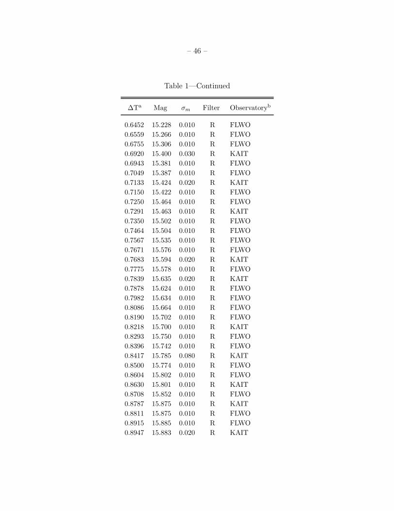
– 46 –

Table 1—Continued


0.6452 15.228 0.010 R FLWO

0.6559 15.266 0.010 R FLWO

0.6755 15.306 0.010 R FLWO

0.6920 15.400 0.030 R KAIT

0.6943 15.381 0.010 R FLWO

0.7049 15.387 0.010 R FLWO

0.7133 15.424 0.020 R KAIT

0.7150 15.422 0.010 R FLWO

0.7250 15.464 0.010 R FLWO

0.7291 15.463 0.010 R KAIT

0.7350 15.502 0.010 R FLWO

0.7464 15.504 0.010 R FLWO

0.7567 15.535 0.010 R FLWO

0.7671 15.576 0.010 R FLWO

0.7683 15.594 0.020 R KAIT

0.7775 15.578 0.010 R FLWO

0.7839 15.635 0.020 R KAIT

0.7878 15.624 0.010 R FLWO

0.7982 15.634 0.010 R FLWO

0.8086 15.664 0.010 R FLWO

0.8190 15.702 0.010 R FLWO

0.8218 15.700 0.010 R KAIT

0.8293 15.750 0.010 R FLWO

0.8396 15.742 0.010 R FLWO

0.8417 15.785 0.080 R KAIT

0.8500 15.774 0.010 R FLWO

0.8604 15.802 0.010 R FLWO

0.8630 15.801 0.010 R KAIT

0.8708 15.852 0.010 R FLWO

0.8787 15.875 0.010 R KAIT

0.8811 15.875 0.010 R FLWO

0.8915 15.885 0.010 R FLWO

0.8947 15.883 0.020 R KAIT

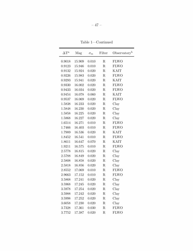
– 47 –

Table 1—Continued


0.9018 15.909 0.010 R FLWO

0.9123 15.946 0.010 R FLWO

0.9132 15.924 0.020 R KAIT

0.9226 15.983 0.020 R FLWO

0.9293 15.941 0.020 R KAIT

0.9330 16.002 0.020 R FLWO

0.9433 16.034 0.020 R FLWO

0.9454 16.078 0.060 R KAIT

0.9537 16.069 0.020 R FLWO

1.5838 16.233 0.020 R Clay

1.5848 16.230 0.020 R Clay

1.5858 16.225 0.020 R Clay

1.5868 16.227 0.020 R Clay

1.6514 16.271 0.010 R FLWO

1.7466 16.403 0.010 R FLWO

1.7989 16.536 0.020 R KAIT

1.8452 16.541 0.010 R FLWO

1.8611 16.647 0.070 R KAIT

1.9211 16.575 0.010 R FLWO

2.5778 16.815 0.020 R Clay

2.5788 16.849 0.020 R Clay

2.5808 16.858 0.020 R Clay

2.5818 16.856 0.020 R Clay

2.8552 17.069 0.010 R FLWO

2.9663 17.152 0.010 R FLWO

3.5868 17.241 0.020 R Clay

3.5968 17.245 0.020 R Clay

3.5978 17.254 0.020 R Clay

3.5988 17.242 0.020 R Clay

3.5998 17.252 0.020 R Clay

3.6058 17.230 0.020 R Clay

3.7328 17.361 0.030 R FLWO

3.7752 17.387 0.020 R FLWO

– 48 –

Table 1—Continued


3.7942 17.408 0.010 R FLWO

3.8192 17.433 0.010 R FLWO

3.8383 17.462 0.010 R FLWO

3.8688 17.491 0.020 R FLWO

4.6008 17.799 0.020 R Clay

4.6048 17.788 0.020 R Clay

4.6058 17.788 0.020 R Clay

4.6068 17.795 0.020 R Clay

4.6088 17.797 0.020 R Clay

4.6098 17.803 0.020 R Clay

4.6348 17.807 0.020 R Clay

4.6368 17.803 0.020 R Clay

4.6388 17.826 0.020 R Clay

4.6504 17.790 0.020 R FLWO

5.6423 17.776 0.020 R FLWO

6.6578 18.253 0.020 R FLWO

6.8776 18.395 0.020 R FLWO

7.6469 18.734 0.030 R FLWO

7.8827 18.750 0.040 R FLWO

8.6440 18.848 0.030 R FLWO

8.6653 18.834 0.040 R FLWO

8.7808 18.845 0.030 R FLWO

8.8830 18.881 0.030 R FLWO

9.6409 18.891 0.030 R FLWO

9.7674 18.935 0.030 R FLWO

9.8631 18.942 0.040 R FLWO

10.6708 19.097 0.040 R FLWO

10.8258 19.050 0.030 R FLWO

11.6529 19.246 0.030 R FLWO

11.6940 19.209 0.030 R FLWO

11.8158 19.258 0.030 R FLWO

12.6858 19.305 0.030 R FLWO

12.8158 19.358 0.040 R FLWO

– 49 –

Table 1—Continued


13.6344 19.414 0.080 R FLWO

13.6590 19.480 0.080 R FLWO

19.6958 19.777 0.040 R FLWO

19.7354 19.807 0.040 R FLWO

19.7822 19.815 0.060 R FLWO

20.7058 19.859 0.040 R FLWO

20.8038 19.937 0.050 R FLWO

20.8398 19.795 0.050 R FLWO

21.6588 19.938 0.030 R FLWO

21.7862 19.949 0.040 R FLWO

21.8729 19.866 0.060 R FLWO

22.6098 19.945 0.050 R LCO40

22.6448 20.017 0.040 R FLWO

22.7344 20.006 0.040 R FLWO

23.6582 20.080 0.030 R FLWO

23.7544 20.043 0.040 R FLWO

24.6514 20.146 0.040 R FLWO

24.8058 20.117 0.030 R FLWO

25.6658 20.158 0.020 R KPNO4m

25.7001 20.142 0.040 R FLWO

25.7098 20.148 0.020 R KPNO4m

25.7178 20.175 0.040 R FLWO

26.6718 20.255 0.040 R FLWO

27.7108 20.320 0.050 R FLWO

28.7200 20.229 0.050 R FLWO

28.7314 20.347 0.060 R FLWO

29.6629 20.422 0.040 R FLWO

29.6781 20.350 0.040 R FLWO

29.6895 20.422 0.050 R FLWO

30.6941 20.478 0.040 R FLWO

30.7201 20.493 0.040 R FLWO

31.7105 20.568 0.040 R FLWO

32.5908 20.549 0.070 R LCO40

– 50 –

Table 1—Continued


32.6581 20.588 0.040 R FLWO

33.6338 20.665 0.030 R KPNO4m

33.8010 20.563 0.060 R FLWO

33.8173 20.657 0.060 R FLWO

34.5648 20.700 0.040 R KPNO4m

34.6919 20.812 0.070 R FLWO

34.7081 20.705 0.050 R FLWO

36.8058 20.875 0.080 R FLWO

37.6631 20.820 0.070 R FLWO

37.6738 20.897 0.050 R FLWO

37.6846 20.823 0.060 R FLWO

38.7300 21.024 0.060 R FLWO

39.6716 21.012 0.070 R FLWO

51.7458 21.553 0.060 R FLWO

52.7058 21.698 0.110 R FLWO

53.7408 21.430 0.080 R FLWO

54.6944 21.309 0.090 R FLWO

57.7163 21.612 0.060 R FLWO

59.7069 21.456 0.070 R FLWO

60.7058 21.618 0.090 R FLWO

0.6470 14.820 0.010 I FLWO

0.6577 14.845 0.010 I FLWO

0.6801 14.896 0.010 I FLWO

0.6959 14.937 0.010 I FLWO

0.6961 14.974 0.030 I KAIT

0.7062 14.981 0.010 I FLWO

0.7155 14.995 0.030 I KAIT

0.7162 15.045 0.010 I FLWO

0.7262 15.053 0.010 I FLWO

0.7313 15.034 0.020 I KAIT

0.7362 15.042 0.010 I FLWO

0.7477 15.103 0.010 I FLWO

0.7580 15.134 0.010 I FLWO

– 51 –

Table 1—Continued


0.7684 15.173 0.010 I FLWO

0.7705 15.133 0.030 I KAIT

0.7788 15.182 0.010 I FLWO

0.7862 15.219 0.030 I KAIT

0.7891 15.225 0.010 I FLWO

0.7995 15.218 0.020 I FLWO

0.8098 15.232 0.020 I FLWO

0.8203 15.287 0.010 I FLWO

0.8259 15.286 0.020 I KAIT

0.8306 15.331 0.010 I FLWO

0.8409 15.352 0.020 I FLWO

0.8440 15.300 0.030 I KAIT

0.8513 15.380 0.010 I FLWO

0.8616 15.420 0.020 I FLWO

0.8652 15.402 0.020 I KAIT

0.8721 15.411 0.020 I FLWO

0.8810 15.424 0.020 I KAIT

0.8824 15.407 0.020 I FLWO

0.8927 15.424 0.020 I FLWO

0.8969 15.471 0.020 I KAIT

0.9031 15.443 0.020 I FLWO

0.9136 15.511 0.020 I FLWO

0.9155 15.534 0.020 I KAIT

0.9239 15.606 0.020 I FLWO

0.9316 15.571 0.040 I KAIT

0.9343 15.648 0.020 I FLWO

0.9446 15.648 0.020 I FLWO

0.9477 15.569 0.030 I KAIT

0.9550 15.649 0.030 I FLWO

1.6542 15.828 0.010 I FLWO

1.7495 15.950 0.010 I FLWO

1.8029 16.044 0.040 I KAIT

1.8481 16.087 0.010 I FLWO

– 52 –

Table 1—Continued


1.8652 16.059 0.070 I KAIT

1.9239 16.123 0.010 I FLWO

2.8581 16.594 0.010 I FLWO

2.9692 16.681 0.020 I FLWO

3.7780 16.957 0.020 I FLWO

3.7970 16.979 0.020 I FLWO

3.8220 16.971 0.020 I FLWO

3.8412 17.014 0.020 I FLWO

3.8717 17.027 0.050 I FLWO

4.6532 17.363 0.020 I FLWO

5.6451 17.319 0.020 I FLWO

5.7205 17.369 0.020 I LCO100

5.7224 17.365 0.020 I LCO100

6.5936 17.830 0.020 I LCO100

6.5956 17.878 0.030 I LCO100

6.6606 17.899 0.030 I FLWO

6.8811 17.968 0.030 I FLWO

7.6504 18.315 0.040 I FLWO

7.8862 18.386 0.050 I FLWO

8.6475 18.473 0.040 I FLWO

8.7844 18.469 0.040 I FLWO

8.8866 18.518 0.050 I FLWO

9.6444 18.595 0.050 I FLWO

9.7709 18.527 0.040 I FLWO

9.8666 18.583 0.060 I FLWO

10.6807 18.741 0.050 I FLWO

10.8158 18.768 0.040 I FLWO

11.6667 18.906 0.040 I FLWO

11.7475 18.938 0.050 I FLWO

11.8441 18.985 0.060 I FLWO

3.6058 15.935 0.020 J LCO40

4.6488 16.449 0.030 J LCO40

5.6552 16.416 0.020 J LCO40

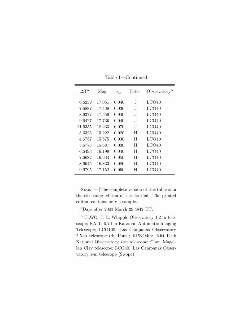
Table 1—Continued


6.6239 17.051 0.040 J LCO40

7.6887 17.438 0.030 J LCO40

8.6377 17.559 0.040 J LCO40

9.6427 17.736 0.040 J LCO40

11.6355 18.233 0.070 J LCO40

3.6325 15.222 0.020 H LCO40

4.6757 15.575 0.030 H LCO40

5.6775 15.687 0.030 H LCO40

6.6493 16.199 0.040 H LCO40

7.6682 16.634 0.050 H LCO40

8.6645 16.833 0.080 H LCO40

9.6795 17.152 0.050 H LCO40

Note. — [The complete version of this table is in

the electronic edition of the Journal. The printed

edition contains only a sample.]

aDays after 2003 March 29.4842 UT.

b FLWO: F. L. Whipple Observatory 1.2-m tele-

scope; KAIT: 0.76-m Katzman Automatic Imaging

Telescope; LCO100: Las Campanas Observatory

2.5-m telescope (du Pont); KPNO4m: Kitt Peak

National Observatory 4-m telescope; Clay: Magel-

lan Clay telescope; LCO40: Las Campanas Obser-

vatory 1-m telescope (Swope)

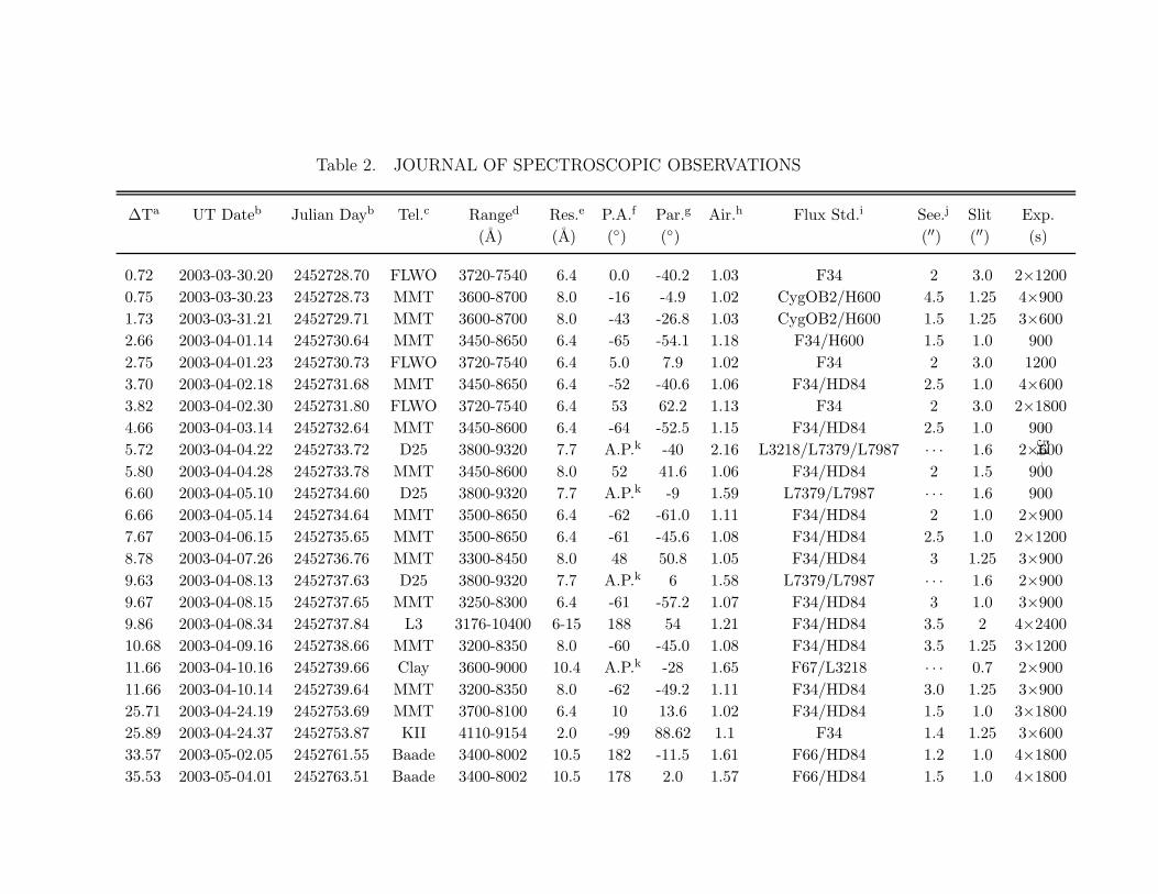
–54

–

Table 2. JOURNAL OF SPECTROSCOPIC OBSERVATIONS

∆Ta UT Dateb Julian Dayb Tel.c Ranged Res.e P.A.f Par.g Air.h Flux Std.i See.j Slit Exp.

(A) (A) () () (′′) (′′) (s)

0.72 2003-03-30.20 2452728.70 FLWO 3720-7540 6.4 0.0 -40.2 1.03 F34 2 3.0 2×1200

0.75 2003-03-30.23 2452728.73 MMT 3600-8700 8.0 -16 -4.9 1.02 CygOB2/H600 4.5 1.25 4×900

1.73 2003-03-31.21 2452729.71 MMT 3600-8700 8.0 -43 -26.8 1.03 CygOB2/H600 1.5 1.25 3×600

2.66 2003-04-01.14 2452730.64 MMT 3450-8650 6.4 -65 -54.1 1.18 F34/H600 1.5 1.0 900

2.75 2003-04-01.23 2452730.73 FLWO 3720-7540 6.4 5.0 7.9 1.02 F34 2 3.0 1200

3.70 2003-04-02.18 2452731.68 MMT 3450-8650 6.4 -52 -40.6 1.06 F34/HD84 2.5 1.0 4×600

3.82 2003-04-02.30 2452731.80 FLWO 3720-7540 6.4 53 62.2 1.13 F34 2 3.0 2×1800

4.66 2003-04-03.14 2452732.64 MMT 3450-8600 6.4 -64 -52.5 1.15 F34/HD84 2.5 1.0 900

5.72 2003-04-04.22 2452733.72 D25 3800-9320 7.7 A.P.k -40 2.16 L3218/L7379/L7987 · · · 1.6 2×600

5.80 2003-04-04.28 2452733.78 MMT 3450-8600 8.0 52 41.6 1.06 F34/HD84 2 1.5 900

6.60 2003-04-05.10 2452734.60 D25 3800-9320 7.7 A.P.k -9 1.59 L7379/L7987 · · · 1.6 900

6.66 2003-04-05.14 2452734.64 MMT 3500-8650 6.4 -62 -61.0 1.11 F34/HD84 2 1.0 2×900

7.67 2003-04-06.15 2452735.65 MMT 3500-8650 6.4 -61 -45.6 1.08 F34/HD84 2.5 1.0 2×1200

8.78 2003-04-07.26 2452736.76 MMT 3300-8450 8.0 48 50.8 1.05 F34/HD84 3 1.25 3×900

9.63 2003-04-08.13 2452737.63 D25 3800-9320 7.7 A.P.k 6 1.58 L7379/L7987 · · · 1.6 2×900

9.67 2003-04-08.15 2452737.65 MMT 3250-8300 6.4 -61 -57.2 1.07 F34/HD84 3 1.0 3×900

9.86 2003-04-08.34 2452737.84 L3 3176-10400 6-15 188 54 1.21 F34/HD84 3.5 2 4×2400

10.68 2003-04-09.16 2452738.66 MMT 3200-8350 8.0 -60 -45.0 1.08 F34/HD84 3.5 1.25 3×1200

11.66 2003-04-10.16 2452739.66 Clay 3600-9000 10.4 A.P.k -28 1.65 F67/L3218 · · · 0.7 2×900

11.66 2003-04-10.14 2452739.64 MMT 3200-8350 8.0 -62 -49.2 1.11 F34/HD84 3.0 1.25 3×900

25.71 2003-04-24.19 2452753.69 MMT 3700-8100 6.4 10 13.6 1.02 F34/HD84 1.5 1.0 3×1800

25.89 2003-04-24.37 2452753.87 KII 4110-9154 2.0 -99 88.62 1.1 F34 1.4 1.25 3×600

33.57 2003-05-02.05 2452761.55 Baade 3400-8002 10.5 182 -11.5 1.61 F66/HD84 1.2 1.0 4×1800

35.53 2003-05-04.01 2452763.51 Baade 3400-8002 10.5 178 2.0 1.57 F66/HD84 1.5 1.0 4×1800

–55

–

Table 2—Continued

∆Ta UT Dateb Julian Dayb Tel.c Ranged Res.e P.A.f Par.g Air.h Flux Std.i See.j Slit Exp.

(A) (A) () () (′′) (′′) (s)

36.55 2003-05-05.03 2452764.53 Baade 6240-9220 5.1 179 180 1.57 HD84 1.5 1.0 4×1800

55.90 2003-05-24.38 2452783.38 KI 3260-9280 8.0 79.9 79.4 1.80 BD28/BD17 1.3 1.5 3×900

Note. — Not all spectra listed in this Table are shown in the paper.

aDays since 2003 March 29.4842 UT.

bMidpoint of observation(s).

cMMT = MMT 6.5m/Blue Channel; FLWO = FLWO 1.5m/FAST; D25 = du Pont 2.5m/WFCCD; L3 = Lick 3m/Kast;

Clay = Magellan 6.5m Clay/LDSS2; KII = Keck II 10m/ESI; Baade = Magellan 6.5m Baade/Boller & Chivens; KI = Keck I

10m/LRIS.

dObserved wavelength range of spectrum. In some cases, the extreme ends are noisy, and are not shown in the figures.

eApproximate spectral resolution (full width at half maximum intensity), typically estimated from night-sky emission lines.

fApproximate average position angle of the spectrograph slit.

gOptimal parallactic angle over the course of the exposures.

hAverage airmass of observations.

iThe standard stars are as follows: BD28 = BD+284211, F34 = Feige 34, H600 = Hiltner 600—Stone (1977), Massey &

Gronwall (1990); F66 = Feige 66, F67 = Feige 67, CygOB2 = Cyg OB2 No. 9—Massey et al. (1988); HD84 = HD 84937, BD17

= BD+474708—Oke & Gunn (1983); L3218 = LTT 3218, L7379 = LTT 7379, L7987 = LTT 7987—Hamuy et al. (1992; 1994).

jApproximate seeing, estimated from the data and observers’ records.

kA.P. = At Parallactic.

–56

–

Table 3. EMISSION LINE RATIOS

log log log log log

([O III] λ5007/[O II] λ3727) ([N II] λ6584/[O II] λ3727) ([O II]+[O III])/Hβ ([N II] λ6584/Hα) Hα/Hβ Hγ/Hβ ([N II] λ6584/[O III] λ5007)

0.2 < −0.9 0.9 < −1.0 3.0 0.4 < −1.3

–57

–

Table 4. GRB/SN FITS

∆Ta Best SNb SN %c Fit Range (A)d Fit Errore SN % Bf SN % Rf

0.75 SN 1997ef +44 5 4242-8000 0.025 2 6

1.73 SN 1997ef +44 5 4242-8000 0.025 2 6

2.66 SN 1997ef +84 2 4348-8000 0.087 1 3

3.70 SN 2002ap +28 2 4348-8000 0.570 1 2

4.66 SN 1997ef +25 6 4236-8000 0.134 2 7

5.80 SN 1997ef -11 1 4348-8000 0.056 1 1

6.66 SN 1998bw +11 8 3950-8000 0.110 4 10

7.67 SN 2002ap +6 6 4348-8000 0.853 3 8

8.78 SN 1998bw -7 13 3906-8000 0.459 11 15

9.67 SN 1998bw -6 26 3920-8000 0.135 21 30

10.68 SN 1997ef -11 19 4348-8000 2.949 14 22

11.66 SN 1998bw -3 38 4092-8000 1.067 29 43

25.80 SN 1998bw +6 61 3950-8000 0.695 46 68

33.57 SN 1998bw +13 63 3622-8000 2.154 45 72

35.53 SN 1998bw +11 86 3950-8000 3.921 76 89

aDays since 2003 March 29.4842 UT.

bSN spectrum that best matches the OT afterglow at this epoch (SN and approximate

phase relative to B-band maximum). Note that the low SN fraction at early times

(∆T = 0.75 − 7.67 days) makes the SN spectrum listed almost arbitrary.

cPercentage of SN component in best-fit spectrum over the fitting range listed.

dSpectral range of the overall fit.

eLeast-squares deviation from fit (not a formal χ2 statistic). Only the relative size of

this number is important.

fRelative contribution of the SN in the broad-band filter indicated, synthesized from

the best-fit, scaled SN spectrum.

Photometry and Spectroscopy of GRB 030329 and Its Associated Supernova 2003dh: The First Two Months

Documents