Development of new methodologies based on ICP techniques for the elemental and isotopic analysis of bioethanol and related samples Carlos Sánchez Rodríguez

Welcome message from author
This document is posted to help you gain knowledge. Please leave a comment to let me know what you think about it! Share it to your friends and learn new things together.
Transcript
Development of new methodologies based on
ICP techniques for the elemental and isotopic
analysis of bioethanol and related samples
Carlos Sánchez Rodríguez
DEPARTAMENTO DE QUÍMICA ANALÍTICA, NUTRICIÓN Y BROMATOLOGÍA
FACULTAD DE CIENCIAS
UNIVERSIDAD DE ALICANTE
DEVELOPMENT OF NEW METHODOLOGIES BASED ON ICP TECHNIQUES FOR THE ELEMENTAL AND
ISOTOPIC ANALYSIS OF BIOETHANOL AND RELATED SAMPLES
CARLOS SÁNCHEZ RODRÍGUEZ
Tesis presentada para aspirar al grado de
DOCTOR POR LA UNIVERSIDAD DE ALICANTE
MENCIÓN DE DOCTOR INTERNACIONAL
PD CIENCIAS EXPERIMENTALES Y BIOSANITARIAS
Dirigida por:
Prof. Dr. JOSÉ LUIS TODOLÍ TORRÓ
Dr. CHARLES PHILIPPE LIENEMANN
La presente Tesis Doctoral ha sido financiada por el centro de investigación IFP Energies Nouvelles (Lyon, France) y una ayuda para la Formación del Profesorado Universitario
(FPU13/01438) concedida por el Ministerio de Educación, Cultura y Deporte.

Dra. DOÑA MARÍA SOLEDAD PRATS MOYA, directora del Departamento de
Química Analítica, Nutrición y Bromatología de la Facultad de Ciencias de la
Universidad de Alicante
Certifica que,
D. CARLOS SÁNCHEZ RODRÍGUEZ ha realizado, bajo la dirección del profesor
Dr. D. JOSÉ LUIS TODOLÍ TORRÓ (Departamento de Química Analítica,
Nutrición y Bromatología. Universidad de Alicante, Alicante, España) y del Dr.
D. CHARLES PHILIPPE LIENEMANN (IFP Energies Nouvelles, Lyon, Francia), el
trabajo correspondiente a la obtención del Grado de Doctor en Ciencias
Experimentales y Biosanitarias (Mención de Doctor Internacional) titulado
DEVELOPMENT OF NEW METHODOLOGIES BASED ON ICP TECHNIQUES FOR
THE ELEMENTAL AND ISOTOPIC ANALYSIS OF BIOETHANOL AND RELATED
SAMPLES
Alicante, marzo de 2018
Fdo. Dra. María Soledad Prats Moya

El profesor Dr. D. JOSÉ LUIS TODOLÍ TORRÓ (Departamento de Química
Analítica, Nutrición y Bromatología. Universidad de Alicante, Alicante,
España) y el Dr. D. CHARLES PHILIPPE LIENEMANN (IFP Energies Nouvelles,
Lyon, Francia), en calidad de directores de la Tesis Doctoral presentada por
D. CARLOS SÁNCHEZ RODRÍGUEZ, conducente a la obtención del Grado de
Doctor en Ciencias Experimentales y Biosanitarias (Mención de Doctor
I te a io al titulada: DEVELOPMENT OF NEW METHODOLOGIES BASED
ON ICP TECHNIQUES FOR THE ELEMENTAL AND ISOTOPIC ANALYSIS OF
BIOETHANOL AND RELATED SAMPLES
Certifican que,
la citada Tesis Doctoral se ha realizado en los laboratorios del Departamento
de Química Analítica, Nutrición y Bromatología de la Universidad de Alicante,
del centro de investigación IFP Energies Nouvelles y del Departamento de
Química de la Universidad de Gante, y que, a su juicio, reúne los requisitos
necesarios y exigidos en este tipo de trabajos.
Alicante, marzo de 2018
Fdo. Prof. Dr. José Luis Todolí Torró
Fdo. Dr. Charles Philippe Lienemann


A mi familia

AGRADECIMIENTOS /
ACKNOWLEDGEMENTS
El simple hecho de estar escribiendo estas palabras indica que mi Tesis Doctoral está
llegando a su fin, o visto de otro modo, que comienzo una nueva etapa como Doctor que
afronto con tanta ilusión como esta que está a punto de acabar. Este es uno de esos
momentos en los que uno no tiene claro si sentirse feliz, por estar cerca de conseguir algo
por lo que tanto ha trabajado, o triste, porque esta fascinante etapa de mi vida se acaba.
Sin embargo, por encima esa dualidad felicidad-tristeza, destaca otro sentimiento del que
no tengo la menor duda: el agradecimiento. Durante este largo e intenso viaje, he tenido
la suerte de conocer muchas personas sin las que esto no habría sido posible, además de
aquellas que ya conocía mucho antes de encontrarme con la investigación, y que son las
responsables de que hoy esté escribiendo estas palabras. Tengo muy claro que unas
cuantas frases no son suficientes para agradecer tantas cosas como me gustaría y estas
personas merecen, pero permitidme intentarlo.
Me gustaría empezar recordando ese momento, ahora ya lejano, en el que todo comenzó.
Siempre recordaré el día en que un profesor del Departamento de Química Analítica me
preguntó si me interesaba empezar a colaborar en tareas de investigación en mis ratos
li es, pa a e si e at aía este u do . Ese p ofeso , u os años ás ta de, se o i tió
en mi Director de Tesis, al que hoy debo todo lo que se sobre investigación. Muchas
gracias José Luis, no solo por tu constante ayuda, tu inestimable apoyo y tus consejos, sino
por darme la oportunidad de descubrir la investigación. Sin embargo, no solo quisiera
darte las gracias por ser un gran Director de Tesis, sino también por ser un gran
compañero, por haber sido capaz de formarme como científico sin renunciar a pasarlo
bien y reírnos juntos. De ti me llevo un mentor y un amigo, ¡gracias!
During this period, I have also been fortunate to work with Charles Philippe Lienemann.
Thank you, Charles Philippe, for your contribution to this PhD, for transferring me your
knowledge and also for the amazing scientific discussions that we have enjoyed. But I
do ’t a t to a k o ledge o ly fo you a ade i help, si e afte so e of y Tha ks,
Cha les Philippe you told e it’s y o k, I’ just doi g y o k . Ho e e , it as ot
your work our bike rides, badminton matches and other nice moments that we have
shared. Thanks for being, in addition to a great PhD advisor, a great colleague.
I would like to express again my gratitude to my supervisors. José Luis and Charles
Philippe, thank you for giving me the opportunity to be part of this wonderful team where
I always felt that I was one more. For me, you will always be a model to follow to become
a great researcher. It has been a pleasure working with you and I hope to continue doing
it in the future.
Gracias a todos los profesores y profesoras del Departamento de Química Analítica,
Nutrición y Bromatología de la Universidad de Alicante, especialmente a Sole, Raquel y
Salva por vuestro apoyo y por compartir esos cafés y comidas que dan fuerza para
continuar el día. Muchas gracias a todos mis compañeros y compañeras del departamento
con las que he compartido tantas cosas estos años. Gracias también a todos los
estudiantes que de un modo u otro me habéis enseñado cosas y especialmente, Sergio,
Borja, Paula y Claudia, con quien he tenido el placer de trabajar más de cerca.
Me gustaría dar las gracias especialmente a aquellas personas que, además de
compañeros y compañeras de trabajo, se han convertido en amigos y amigas. Phanie,
Águeda, Ángela (y Vicen), Juan Pedro (y Sara), Silvia (y Josemi), gracias por aguantarme
día a día, con lo complicado que eso puede resultar en ciertas ocasiones.
Gracias al resto de amigos y amigas dispersos por el resto de departamentos de Química,
especialmente a Manu, con quien tengo la suerte de compartir vivencias y cafés desde
hace unos 15 años, y a los que me habéis sacado del laboratorio para llevarme de cena,
comida o a una pista de pádel o futbol sala. Gracias también a Mayte y Clemente, por
ayudarme en el ICP-MS y el ICP-OES siempre que lo he necesitado y por permitir que los
Agradecimientos/Acknowledgements
SSTTI sean mi segunda casa. Gracias a Diego por el placer de compartir contigo congresos
y otras experiencias, espero que sean los primeros de muchos.
Y finalmente, para acabar con los amigos que la (bio)Química me ha dado, muchas gracias
a Boby y Aída por esas cenas, que se pasan volando hablando de todo y riéndonos de
todos. Parece ser que las próximas cenas serán en Umeå, pero podéis contar conmigo.
Thanks also to the research center IFPEN. First, for the financial support; and, second,
because during my stays in its laboratories I met amazing people. Thanks to all the
technician of the Physics and Analysis Division for helping me. I would like to thank also
Sylvain Carbonneaux for his support and Fabien Chainet for a lot of good times that we
enjoyed together and your help in Lyon.
I would like to thank also Prof. Frank Vanhaecke and the A&MS research group (Ghent
University) for allowing me to discover other labs, other ways of working and doing
science and for giving me the opportunity of discovering the wonderful world of isotopic
analysis, particularly my office mates (Sara and Lieve) and the Spanish team. Charo, Marta,
Ana y Edu, muchas gracias por la ayuda que, desde el primer día, me brindasteis. Gracias
por la compañía en las largas noches de Neptune, los cafés en el S12 y los grandes ratos
fue a de él. “ois g a des i estigado es, pe o toda ía sois ejo es a igos… y yo te go la
suerte de conocer ambas cosas.
Pero si estoy cerca de ser doctor, no se debe únicamente a los últimos años. Es por ello,
que quiero agradecer a mi familia la inestimable ayuda que me han dado en estos 28 años.
Aunque lo he pensado mucho últimamente, no sé si seré capaz de plasmar en unas
simples palabras todo lo que tengo que agradecer a mis padres, Herminio y Juana. Muchas
gracias a los dos por darme todo sin pedir nada a cambio, por apoyarme en todas mis
decisiones sin cuestionarlas en ningún momento y por haberme formado como persona.
Gracias a mis hermanos, Hermi y Javi, y cuñadas, Mari Carmen y Mayte, por estar siempre
a mi lado disfrutando de los buenos momentos y, sobre todo, pasando los no tan buenos,
por escucharme cuando lo he necesitado. Gracias a todos y todas, simplemente por ser
mi familia. Dicen que la familia no se escoge; y yo digo que, si pudiera escogerla, escogería
exactamente la que tengo.
Puede parecer que me olvido de parte de mi familia, pero en realidad quería guardarles
un párrafo propio. Gracias a mis sobrinos y sobrinas, Javier, Jaime, Carla y Natalia. Sin
saberlo, habéis sido un pilar fundamental de esta Tesis. Gracias a los cuatro por hacerme
sonreír en los malos momentos, por darme esa alegría que lleváis dentro. Vuestras
llamadas por Skype y esos audios de WhatsApp durante las estancias dan ilusión y fuerzas
para seguir adelante.
Y mención especial, y por eso le he reservado el último agradecimiento de mi Tesis,
merece una persona con la que me siento formando un tándem perfecto y me
comprende, en ocasiones sin que diga ni una sola palabra. Gracias Ainhoa, por tu apoyo
incondicional, por apoyarme en todas las decisiones que he tomado durante esta Tesis,
incluso cuando algunas implican estar lejos de ti mucho tiempo. Simplemente, gracias por
estar conmigo siempre. Como tú bien sabes, todo llega.
Por todos estos motivos, y aunque sé que estas palabras no son suficientes para expresar
lo ue ha éis o t i uido a esta Tesis… GRACIAS
For all these reasons, although I know that these words are not enough to express your
o t i utio to this PhD…THANK“
List of contents
i
List of contents
List of acronyms and abbreviatures ................................................................................... vii
List of bioethanol samples ................................................................................................ xiii
List of figures ...................................................................................................................... xv
List of tables ....................................................................................................................... xix
RESUMEN ............................................................................................................................. 1
ABSTRACT ........................................................................................................................... 15
1 Inductively coupled plasma instrumentation ............................................................. 27
1.1 Sample introduction systems .............................................................................. 29
1.1.1 Nebulizers .................................................................................................... 29
1.1.2 Spray chambers ............................................................................................ 32
1.1.3 Special sample introduction systems .......................................................... 36
1.2 Plasma source...................................................................................................... 39
1.3 ICP-OES Perkin Elmer Optima 4300DV. ............................................................... 41
1.3.1 Transfer optics ............................................................................................. 42
1.3.2 Wavelength dispersive device ..................................................................... 43
1.3.3 Detector ....................................................................................................... 44
1.4 ICP-mass spectrometry (ICP-MS). General points............................................... 45
1.4.1 Interface ....................................................................................................... 46
1.4.2 Ion focusing system ..................................................................................... 46
1.4.3 Mass spectrometer ...................................................................................... 47
1.5 ICP-QMS Agilent 7700x ....................................................................................... 48
1.5.1 Collision cell. ................................................................................................ 50
1.5.2 Quadrupole filter ......................................................................................... 53
1.5.3 Detector ....................................................................................................... 55
ii
1.6 MC-ICP-MS Thermo Neptune. ............................................................................. 56
1.6.1 Double-focusing mass spectrometer ........................................................... 57
1.6.2 Detector ....................................................................................................... 60
1.6.3 Removal of interferences in MC-ICP-MS ..................................................... 60
1.6.4 Correction for instrumental mass discrimination ........................................ 61
1.7 References ........................................................................................................... 64
PUBLISHED WORKS / TRABAJOS PUBLICADOS .................................................................. 73
2 Metal and metalloids determination in biodiesel and bioethanol ............................ 75
2.1 Abstract ............................................................................................................... 79
2.2 General Introduction ........................................................................................... 80
2.3 Fundamental studies ........................................................................................... 83
2.3.1 Aerosol generation ...................................................................................... 83
2.3.2 Aerosol transport ......................................................................................... 86
2.3.3 Plasma effects. ............................................................................................. 88
2.3.4 Spectral interferences .................................................................................. 91
2.4 Biodiesel .............................................................................................................. 93
2.4.1 Synthesis and presence of metals. Importance of their determination. .... 94
2.4.2 Analysis by ICP techniques ........................................................................... 96
2.4.3 Analysis by additional techniques .............................................................. 103
2.4.4 Comparison among techniques ................................................................. 121
2.4.5 Standards for the analysis of biodiesel ...................................................... 124
2.5 Bioethanol ......................................................................................................... 126
2.5.1 Synthesis and presence of metals. Importance of their determination. .. 126
2.5.2 Analysis by ICP techniques ......................................................................... 128
2.5.3 Analysis by other techniques ..................................................................... 133
2.5.4 Speciation ................................................................................................... 135
List of contents
iii
2.5.5 Comparison among techniques. ................................................................ 150
2.5.6 Standards for the analysis of bioethanol ................................................... 151
2.6 Conclusions........................................................................................................ 154
2.7 Acknowledgements ........................................................................................... 156
2.8 References ......................................................................................................... 157
3 Metal and metalloid determination in bioethanol through inductively coupled
plasma-optical emission spectroscopy ............................................................................ 183
3.1 Abstract ............................................................................................................. 187
3.2 Introduction....................................................................................................... 188
3.3 Experimental ..................................................................................................... 189
3.3.1 Solutions and samples ............................................................................... 189
3.3.2 Instrumentation ......................................................................................... 191
3.4 Results and discussion ....................................................................................... 192
3.4.1 Drop size distribution ................................................................................. 192
3.4.2 Effect of the sample pre-treatment ........................................................... 193
3.4.3 Effect of hTISIS temperature on sensitivity and matrix effects in segmented
flow injection ............................................................................................................ 194
3.4.4 Effect of hTISIS temperature on sensitivity and matrix effects in continuous
aspiration mode ........................................................................................................ 199
3.4.5 Limits of detection ..................................................................................... 199
3.5 Recovery tests ................................................................................................... 201
3.6 Analysis of real samples .................................................................................... 201
3.6.1 hTISIS-ICP-OES-segmented injection ......................................................... 201
3.6.2 hTISIS-ICP-OES-continuous injection ......................................................... 203
3.6.3 Comparison between continuous and segmented flow injection............. 203
3.7 Conclusions........................................................................................................ 206
iv
3.8 Acknowledgements ........................................................................................... 206
3.9 References ......................................................................................................... 208
4 Analysis of bioethanol samples through Inductively Coupled Plasma-Mass
Spectrometry with a total sample consumption system ................................................. 213
4.1 Abstract ............................................................................................................. 217
4.2 Introduction....................................................................................................... 218
4.3 Experimental ..................................................................................................... 219
4.3.1 Solutions and samples ............................................................................... 219
4.3.2 Instrumentation ......................................................................................... 220
4.4 Results and Discussion ...................................................................................... 222
4.4.1 Analyte transport efficiency....................................................................... 222
4.4.2 Analytical figures of merit .......................................................................... 224
4.4.3 Matrix effects caused by ethanol .............................................................. 228
4.4.4 Recovery tests ............................................................................................ 236
4.4.5 Analysis of bioethanol real samples .......................................................... 239
4.5 Conclusions........................................................................................................ 242
4.6 Acknowledgements ........................................................................................... 242
4.7 References ......................................................................................................... 243
5 Evolution of the metal and metalloid content along the bioethanol production
process ............................................................................................................................. 247
5.1 Abstract ............................................................................................................. 251
5.2 Introduction....................................................................................................... 252
5.3 Experimental ..................................................................................................... 254
5.3.1 Reagents and standards ............................................................................. 254
5.3.2 Bioethanol production process and samples ............................................ 255
5.3.3 Samples preparation. ................................................................................. 256
List of contents
v
5.3.4 Instrumentation. ........................................................................................ 257
5.3.5 Method validation and samples analysis. .................................................. 259
5.4 Results and discussion. ...................................................................................... 259
5.4.1 Evaluation of the four sample preparation methods. ............................... 259
5.4.2 Analytical figures of merit. ......................................................................... 263
5.4.3 Recovery test. ............................................................................................ 264
5.4.4 Analysis of real samples. Fate of metals and metalloids along the production
process. .................................................................................................................... 265
5.5 Conclusions........................................................................................................ 274
5.6 Acknowledgements ........................................................................................... 274
5.7 References ......................................................................................................... 275
6 Direct lead isotopic analysis of bioethanol by means of multi-collector ICP-mass
spectrometry with a total consumption sample introduction system ............................ 279
6.1 Abstract ............................................................................................................. 283
6.2 Introduction....................................................................................................... 285
6.3 Experimental ..................................................................................................... 287
6.3.1 Aqueous standards and certified reference materials .............................. 287
6.3.2 Ethanol-water standards and bioethanol samples .................................... 288
6.3.3 Instrumentation and measurements ......................................................... 289
6.4 Results and discussion ....................................................................................... 292
6.4.1 Effect of sample introduction system and skimmer type on the sensitivity ...
.................................................................................................................... 292
6.4.2 Effect of sample introduction system and skimmer type on the isotope ratio
precision and accuracy ............................................................................................. 294
6.4.3 Effect of sample introduction system and skimmer type on the mass bias
correction. ................................................................................................................ 297
6.4.4 Effect of hTISIS temperature on the mass bias correction ........................ 300
vi
6.4.5 Robustness of the method to real matrices .............................................. 302
6.4.6 Lead isotope ratios in bioethanol .............................................................. 303
6.5 Conclusions........................................................................................................ 305
6.6 Acknowledgements ........................................................................................... 306
6.7 References ......................................................................................................... 307
UNPUBLISHED WORKS / TRABAJOS NO PUBLICADOS ..................................................... 313
7 Determination of volatile organic compounds in bioethanol by means of GC-FID and
GC-MS .............................................................................................................................. 315
7.1 Introduction....................................................................................................... 317
7.2 Experimental ..................................................................................................... 319
7.2.1 Gas Chromatography-Flame Ionization Detector (GC-FID) ....................... 319
7.2.2 Gas Chromatography-Mass Spectrometry (GC-MS) .................................. 319
7.2.3 Standards and samples. ............................................................................. 320
7.3 Results ............................................................................................................... 321
7.3.1 Quantification of major volatile compounds in bioethanol real samples by
means of GC-FID ....................................................................................................... 321
7.3.2 Semi-quantitative determination of major, minor and trace volatile
compounds by means of GC-MS .............................................................................. 330
7.4 Conclusions........................................................................................................ 350
7.5 References ......................................................................................................... 352
GENERAL CONCLUSIONS .................................................................................................. 355
CONCLUSIONES GENERALES ............................................................................................ 361
FUTURE STUDIES .............................................................................................................. 367
SCIENTIFIC IMPACT .......................................................................................................... 371
List of acronyms and abbreviatures
vii
List of a ro y s a d a re iatures
α Significance level
AC Alternating current
ASI Air - segmented injection
AAS Atomic absorption spectrometry
AFE Anhydrous fuel ethanol
ANP National Agency of Petroleum
ASTM American Society for Testing and Materials
ASV Anodic stripping voltammetry
BEC Background equivalent concentration
b.p. Boiling point
BTEX Benzene, toluene, ethylbenzene and xylene
CCD Charge - coupled device
CDA Chelidamic acid
CID Charge - injection device
CRI Collision - reaction interface
CRC Collision - reaction cell
CRM Certified reference material
CSA Continuous sample aspiration
CTD Charge - transfer device
CV-AFS Cold vapor - atomic fluorescence spectroscopy
viii
ETAAS Electrothermal atomic absorption spectroscopy
D3,2 Sauter mean diameter
D50 Median of aerosol volume drop size distribution
DC Direct current
DCC Dynamic collision cell
DPA Diphenylamine
DRC Dynamic reaction cell
εn Analyte transport efficiency
Ei First ionization energy
ETAAS Electrothermal atomic absorption spectroscopy
EtOH Ethanol
ETV Electrothermal vaporization
FAAS Flame atomic absorption spectrometry
FAEE Fatty acid ethyl esters
FAES Flame atomic emission spectrometry
FAME Fatty acid methyl esters
GC Gas chromatography
GC-FID Gas chromatography - flame ionization detector
GC-MS Gas chromatography - mass spectrometry
GHG Greenhouse gas
HDPE High-density polyethylene
HFE Hydrated fuel ethanol
HMI High matrix introduction system/device
List of acronyms and abbreviatures
ix
HPLC High - performance liquid chromatography
HR High resolution
HR-CS-AAS High resolution continuum source graphite furnace atomic
absorption spectrometry
hTISIS High temperature torch integrated sample introduction system
IC Ion chromatography
ICP Inductively coupled plasma
ICP-MS Inductively coupled plasma - mass spectrometry
ICP-MS/MS Inductively coupled plasma - tandem mass spectrometry
ICP-OES Inductively coupled plasma - optical emission spectroscopy
ICP-QMS Inductively coupled plasma - quadrupole mass spectrometry
ICP-QQQ Inductively coupled plasma - triple quadrupole
ICP-SFMS Inductively coupled plasma - sector field mass spectrometry
ICP-TOF-MS Inductively coupled plasma - time of flight - mass spectrometry
ID Isotope dilution
IFPEN Institute Français du Pétrole Energies Nouvelles
IH In - house standard
Ir or Irel Relative intensity
KED Kinetic energy discrimination
LA Laser ablation
LHR Solid lignin hydrolysate residue
LOD Limit of detection
LOQ Limit of quantification
x
LR Low resolution
m/z Mass to charge ratio
MC-IPC-MS Multi-collector - inductively coupled plasma - mass spectrometry
MCN Microconcentric nebulizer
MDL Method detection limit
MIP-OES Microwave induced plasma - optical emission spectroscopy
MR Medium resolution
MTEB Methyl tert-butyl ether
MW Microwave
N or n Number of replicants
ne Electron number density
NAZ Normal analytical zone
NIST National institute for standards and technology
ORS Octopole reaction system
PAR 4-(2-pyridazo)resorcinol
PDA Photodiode array
PFA Perfluoroalkoxy
PP Polypropilene
Ppb Parts per billion
ppm Parts per million
PPN Parallel - path nebulizer
PTFE Polytetrafluoroethylene
QC Quality control
List of acronyms and abbreviatures
xi
Qg Nebulizer gas flow rate
R Resistivity
R Resolution
Rexp Measured isotope ratio
Rtrue True isotope ratio
RF Radio – frequency
RSD Relative standard deviation
RT Room temperature
Sb or sb Blank standard deviation
SD or s Standard deviation
SF-ICP-MS Sector field - inductively coupled plasma - mass spectrometry
SSB Sample - standard bracketing approach
SSF Simultaneous saccharification and fermentation
T Temperature
TEA Triethylamine
THGA Transversely heated graphite atomizer
TIC Total ions current
TIMS Thermal ionization mass spectrometry
TMAH Tetramethylammonium hydroxide
UNGDA Union Nationale de Groupements de Distillateurs d'Alcool
USN Ultrasonic nebulizer
USN-MD-ICPOES Ultrasonic nebulizer and membrane desolvator inductively
coupled plasma optical emission
xii
v/v volume/volume dilution
VOCs Volatile organic compounds
w/w weight/weight dilution
w/v Weight/volume dilution
Wtot Mass of analyte transported
WCAES Tungsten coil atomic emission spectrometry
List of bioethanol samples
xiii
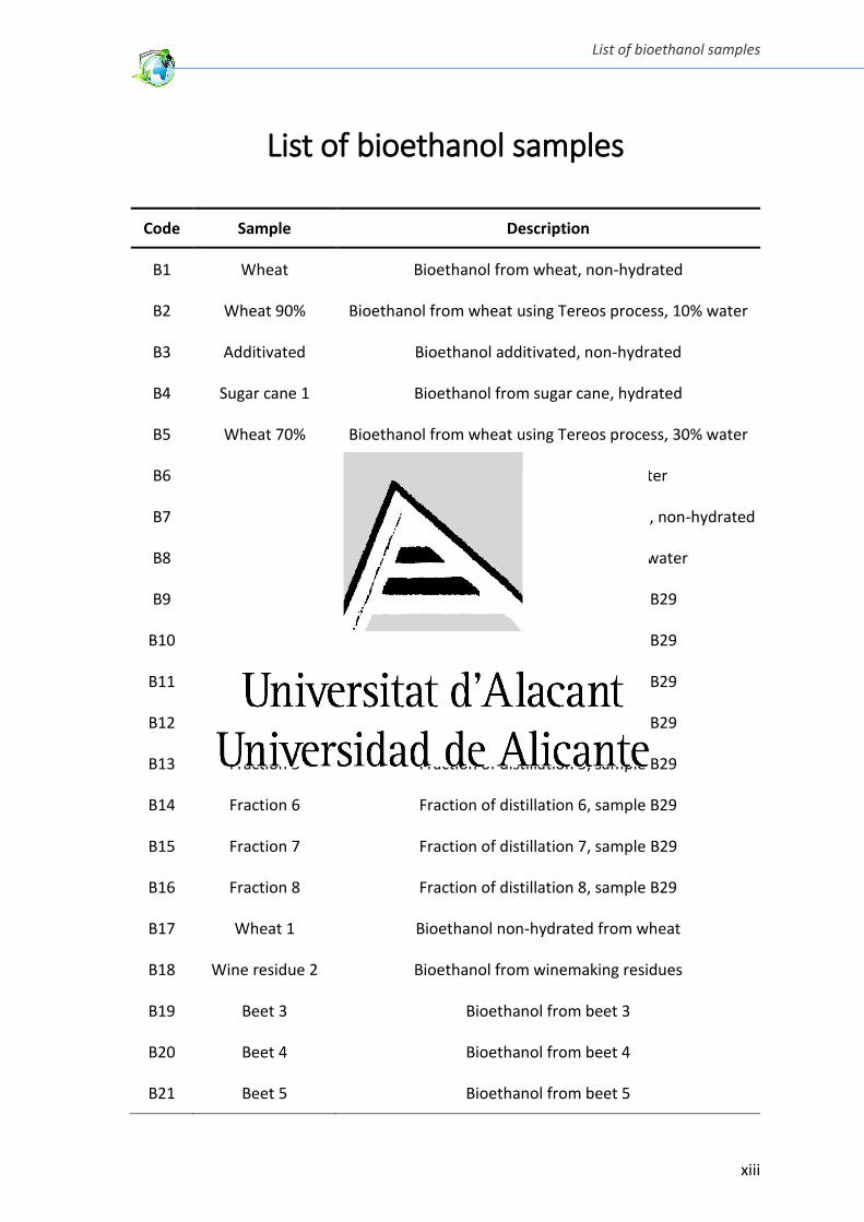
List of ioetha ol sa ples
Code Sample Description
B1 Wheat Bioethanol from wheat, non-hydrated
B2 Wheat 90% Bioethanol from wheat using Tereos process, 10% water
B3 Additivated Bioethanol additivated, non-hydrated
B4 Sugar cane 1 Bioethanol from sugar cane, hydrated
B5 Wheat 70% Bioethanol from wheat using Tereos process, 30% water
B6 Wheat 96% Bioethanol from wheat, 4% water
B7 Wheat + Beet Bioethanol from mixture of wheat and beet, non-hydrated
B8 Sugar cane 2 Bioethanol from sugar cane, 40% water
B9 Fraction 1 Fraction of distillation 1, sample B29
B10 Fraction 2 Fraction of distillation 2, sample B29
B11 Fraction 3 Fraction of distillation 3, sample B29
B12 Fraction 4 Fraction of distillation 4, sample B29
B13 Fraction 5 Fraction of distillation 5, sample B29
B14 Fraction 6 Fraction of distillation 6, sample B29
B15 Fraction 7 Fraction of distillation 7, sample B29
B16 Fraction 8 Fraction of distillation 8, sample B29
B17 Wheat 1 Bioethanol non-hydrated from wheat
B18 Wine residue 2 Bioethanol from winemaking residues
B19 Beet 3 Bioethanol from beet 3
B20 Beet 4 Bioethanol from beet 4
B21 Beet 5 Bioethanol from beet 5
xiv
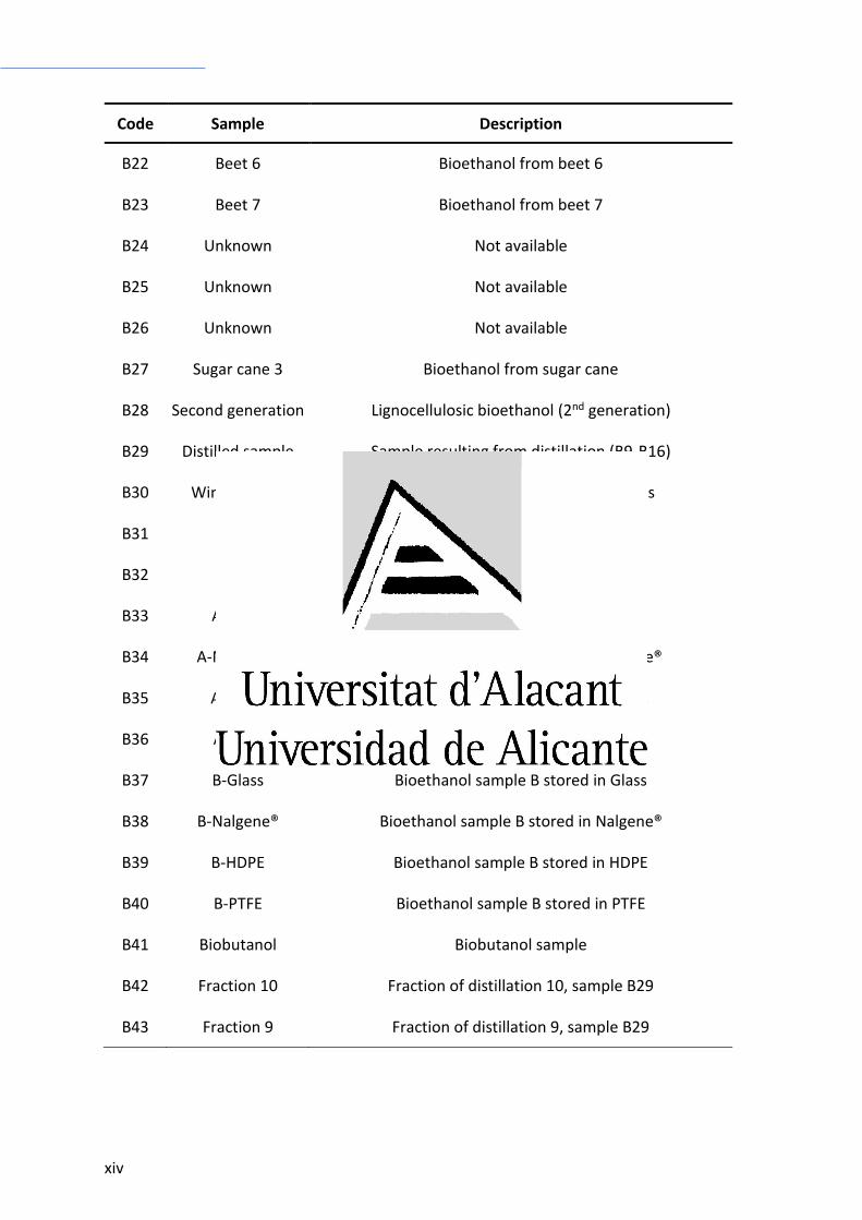
Code Sample Description
B22 Beet 6 Bioethanol from beet 6
B23 Beet 7 Bioethanol from beet 7
B24 Unknown Not available
B25 Unknown Not available
B26 Unknown Not available
B27 Sugar cane 3 Bioethanol from sugar cane
B28 Second generation Lignocellulosic bioethanol (2nd generation)
B29 Distilled sample Sample resulting from distillation (B9-B16)
B30 Wine residue Bioethanol from winemaking residues
B31 Cereal Bioethanol from cereal
B32 Beet Bioethanol from beet
B33 A-Glass Bioethanol sample A stored in glass
B34 A-Nalgene® Bioethanol sample A stored in Nalgene®
B35 A-HDPE Bioethanol sample A stored in HDPE
B36 A-PTFE Bioethanol sample A stored in PTFE
B37 B-Glass Bioethanol sample B stored in Glass
B38 B-Nalgene® Bioethanol sample B stored in Nalgene®
B39 B-HDPE Bioethanol sample B stored in HDPE
B40 B-PTFE Bioethanol sample B stored in PTFE
B41 Biobutanol Biobutanol sample
B42 Fraction 10 Fraction of distillation 10, sample B29
B43 Fraction 9 Fraction of distillation 9, sample B29
List of figures
xv
List of figures
Figure 1.1. Schemes of the most used pneumatic nebulization devices ........................... 30
Figure 1.2. Detailed scheme of a concentric nebulizer. .................................................... 31
Figure 1.3. Scheme of the aerosol transport phenomena in a sample introduction system
consisting of a concentric nebulizer in combination with a double-pass spray chamber
(Scott) ................................................................................................................................. 33
Figure 1.4.Conventional spray chamber designs ............................................................... 35
Figure 1.5. Schematic description of two commercially available desolvation systems ... 37
Figure 1.6. Scheme (a) and picture (b) of the hTISIS sample introduction system. .......... 38
Figure 1.7. (a) Scheme the of torch, coil and plasma and (b) picture of the plasma
generated in an ICP-MS Agilent 7700x spectrometer. ...................................................... 40
Figure 1.8. Scheme of the optic and detection systems of the ICP-OES Perkin Elmer
4300DV. .............................................................................................................................. 42
Figure 1.9. Plasma viewing modes. (a) Radial or side-on viewing and (b) axial or end-on
viewing. .............................................................................................................................. 43
Figure 1.10. Scheme of the operation principle of a CCD detector ................................... 44
Figure 1.11. General scheme of an ICP-MS instrument..................................................... 45
Figure 1.12. Sampler cone and skimmer ........................................................................... 46
Figure 1.13. Detailed scheme of the ICP-MS Agilent 7700x used in chapters 4 and 5 ...... 49
Figure 1.14. Collision-cell operation principle ................................................................... 53
Figure 1.15. Operation principle of a quadrupole mass filter ........................................... 53
Figure 1.16. The combination of the high-mass (a) and low mass (b) filters resulting the
bandpass filter (c) .............................................................................................................. 55
Figure 1.17. Scheme of the MC-ICP-MS Thermo Neptune used in chapter 6. .................. 57
Figure 1.18. Operation principle of magnetic (a) and electrostatic (b) sectors ................ 58
Figure 1.19. Nier-Johnson double-focusing setup ............................................................. 60
Figure 2.1. Sauter mean diameter (D3,2) for primary aerosols generated by a conventional
pneumatic concentric nebulizer working with 19 different bioethanol samples (A-S). .... 86
xvi
Figure 2.2. Spectral survey of the visible emission from de ICP loaded with methanol for
several observations heights. Cyanide radical (410-430 nm) and diatomic carbon (450-520
nm) ..................................................................................................................................... 92
Figure 2.3. Techniques employed for the determination of several metals in biodiesel
samples and number of studies dealing with the determination of each one of the
elements .......................................................................................................................... 123
Figure 2.4. General flow chart of bioethanol production process from lignocelulosic
biomass (second generation) ........................................................................................... 127
Figure 2.5. Techniques employed for the determination of several metals in bioethanol
samples and number of studies dealing with the determination of each one of the
elements .......................................................................................................................... 151
Figure 2.6. Main elements found in real biodiesel and ethanol fuel samples ................ 155
Figure 3.1. D50 of primary aerosols for solutions containing different percentage in
ethanol ............................................................................................................................. 193
Figure 3.2. Peaks for Mn 257.610 and Ar 420.069 and magnesium ratio in the maximum
of the peak for several water-ethanol mixtures at: (a) room temperature; (b) 200°C; (c)
350°C and (d) 400°C ......................................................................................................... 196
Figure 3.3. Relative intensity under discrete sample injection versus the hTISIS
temperature ..................................................................................................................... 198
Figure 4.1. Analyte mass leaving the spray chamber per unit of time (Wtot) normalized
with respect to that measured when the ethanol concentration is 50% versus hTISIS
temperature. .................................................................................................................... 223
Figure 4.2. Effect of the sample introduction system and hTISIS temperature on the signal.
(a) 55Mn; (b) 111Cd. ........................................................................................................... 225
Figure 4.3. Relative intensity variation (taking the 50% ethanol solution as reference)
versus the hTISIS temperature for two different matrices under the air-segmented
injection mode ................................................................................................................. 229
Figure 4.4. Doubly charged ion (a) and oxide ratios (b) for the two sample introduction
systems and several hTISIS temperatures. Air segmented mode. .................................. 230
Figure 4.5. Effect of the chamber walls temperature on the extent of matrix effects. .. 232
Figure 4.6. ICP-MS radial plasma profiles obtained for two different temperatures and
three different solutions .................................................................................................. 234
List of figures
xvii
Figure 4.7. ICP-MS axial plasma profiles obtained for two different temperatures and three
different solutions ............................................................................................................ 236
Figure 4.8. Recoveries found for four real bioetanol spiked samples ............................. 237
Figure 4.9. Elemental concentrations found for several bioethanol samples following five
different procedures ........................................................................................................ 238
Figure 5.1. Scheme of bioethanol production process studied in the present work. ..... 256
Figure 5.2. Recoveries obtained for twelve spiked samples ........................................... 264
Figure 5.3. Evolution of metals along bioethanol production process from the beginning
until the end of the sampling campaign. Sugar factory 1 ................................................ 268
Figure 5.4. Evolution of major metals along bioethanol production process from the
beginning until the end of the sampling campaign of Sugar factory 2............................ 272
Figure 5.5. Evolution of minor metals along bioethanol production process from the
beginning until the end of the sampling campaign of Sugar factory 2............................ 273
Figure 6.1. Effect of ICP-MS interface (a) and introduction system (b) on the sensitivity293
Figure 6.2. Effect of lead concentration on accuracy and precision (H-type skimmer) .. 296
Figure 6.3. Effect of the matrix composition on the effectiveness of mass bias correction
via a combination of internal correction (based on admixed Tl) and external correction
using a Pb standard solution in 75% ethanol for the different skimmer types and sample
introduction systems under optimum conditions ........................................................... 299
Figure 6.4. Effect of hTISIS temperature on the effectiveness of mass bias correction . 301
Figure 6.5. 208Pb/206Pb ratio obtained for spiked bioethanol and ethanol samples with 5
µg L-1 of IH-Pb ................................................................................................................... 303
Figure 6.6. Three-isotopes plot for bioethanol samples coming from different raw
materials .......................................................................................................................... 305
Figure 7.1. Chromatogram obtained under optimum conditions for the standard
containing 2,000 mg L-1 of ten analytes in ethanol ......................................................... 322
Figure 7.2. Recoveries for three samples spiked with 200 mg L-1 of each analyte ......... 324
Figure 7.3. Effect of the distillation step. Chromatograms obtained for the different
distillation fractions. ........................................................................................................ 327
Figure 7.4. Scheme of the samples analyzed and compounds identified by means of GC-
MS. ................................................................................................................................... 331
xviii
Figure 7.5. Reactions that take place in bioethanol. (a) generation of FAEE from TAG and
ethanol; (b) production of FAEE from fatty acids and ethanol; (c) generation of 1,1-
diethoxyethane from ethanol and acetaldehyde. ........................................................... 333
Figure 7.6. Frequency of identification of each analyte when n 3. ................................ 344
Figure 7.7. Number of compounds found in the samples by GC-MS. ............................. 347
Figure 7.8. Chromatograms obtained for distillation fractions ...................................... 348
Figure 7.9. Chromatograms obtained for different raw materials .................................. 349
Figure A.1. Scheme of future studies………………………………………………………………………….. 6
List of tables
xix
List of ta les
Table 1.1. Comparison of the three types of mass spectrometers used in ICP-MS .......... 48
Table 1.2. Examples of typical interferences in ICP-MS classified by categories.. ............ 51
Table 2.1. Standard specifications and maximum allowable levels of metals and
metalloids........................................................................................................................... 81
Table 2.2. Biodiesel and bioethanol based products CRMs. ............................................. 82
Table 2.3. Density, viscosity and surface tension at 20°C for the different samples. ....... 84
Table 2.4. Summary of the limits of detection and found concentrations obtained in
biodiesel samples by several authors. ............................................................................. 109
Table 2.5. List of standards for the elemental determination of biodiesel samples. ...... 125
Table 2.6. Summary of the limits of detection and found concentrations obtained in fuel
ethanol samples by several authors ................................................................................ 136
Table 2.7. Standards for the elemental determination in ethanol employed for fuel
applications. ..................................................................................................................... 152
Table 3.1. Physical properties for a series of samples with different ethanol content... 190
Table 3.2. ICP-OES operating conditions. ........................................................................ 192
Table 3.3. Limits of detection (ng mL-1) obtained in both Injection methodologies. ...... 200
Table 3.4. Found concentrations (in ng mL-1) in bioethanol real samples through hTISIS-
ICP-OES in segmented flow injection.. ............................................................................. 202
Table 3.5. Found concentrations (in ng mL-1) in bioethanol real samples through hTISIS-
ICP-OES in continuous injection. ...................................................................................... 204
Table 4.1. ICP-MS Agilent 7700x operating conditions. .................................................. 221
Table 4.2. Limits of detection for 50% ethanol/water mixtures and different sample
introduction systems in air-segmented injection mode. ................................................. 226
Table 4.3. Found concentrations (in ng mL-1) in real bioethanol samples by means of the
hTISIS-ICP-MS in continuous aspiration ........................................................................... 240
Table 5.1. ICP-MS operating conditions. .......................................................................... 258
Table 5.2. Main elements concentration (mg kg-1) determined for the CRM DC73349 by
using the four acid assisted digestion protocols evaluated ............................................ 261
xx
Table 5.3. Main elements concentration (mg kg-1) for the CRM SRM 1575a by using the
four acid assisted digestion protocols evaluated ............................................................ 262
Table 5.4. Limits of detection (in mg kg-1) obtained for real samples. ............................ 263
Table 6.1. Conditions used for isotope ratio measurements .......................................... 291
Table 6.2. Internal and external precision ....................................................................... 295
Table 7.1. GC-FID operating conditions and column characteristics. .............................. 319
Table 7.2. GC-MS operating conditions and column characteristics. .............................. 320
Table 7.3. Interday and intraday precisions for a multi-compound standard. ............... 323
Table 7.4. Summary of the analytes found in bioethanol real samples .......................... 325
Table 7.5. Concentrations (in mg L-1) of organic pollutants found in different distillation
fraction ............................................................................................................................. 326
Table 7.6. Concentrations (in mg L-1) of organic pollutants found in samples obtained from
different raw materials .................................................................................................... 329
Table 7.7. Concentrations (in mg L-1) of organic pollutants found in samples obtained from
different raw materials with different water content, second generation bioethanol and
biobutanol ........................................................................................................................ 330
Table 7.8. Alcohols found by GC-MS in the bioethanol samples. .................................... 335
Table 7.9. Aldehydes and ketones found by GC-MS in the bioethanol samples. ............ 336
Table 7.10. Esters found by GC-MS in the bioethanol samples. ...................................... 337
Table 7.11. Ethers found by GC-MS in the bioethanol samples. ..................................... 338
Table 7.12. Hydrocarbons found by GC-MS in the bioethanol samples. ......................... 339
Table 7.13. Aromatic hydrocarbons found by GC-MS in the bioethanol samples. ......... 340
Table 7.14. Nitrogen compounds found by GC-MS in the bioethanol samples. ............. 341
Table 7.15. Organic acids found by GC-MS in the bioethanol samples. .......................... 341
Table 7.16. Furane derivates found by GC-MS in the bioethanol samples. .................... 342
Table 7.17. Other organic compounds found by GC-MS in the bioethanol samples. ..... 342

RESUMEN

Resumen
3
La presente Tesis Doctoral, desarrollada en el Departamento de Química Analítica,
Nutrición y Bromatología de la Universidad de Alicante, en colaboración con el centro de
investigación francés IFP Energies Nouvelles (IFPEN), se centra en el desarrollo de nuevas
metodologías analíticas para el análisis elemental (cuantificación de metales) y el análisis
isotópico de muestras de bioetanol, así como de muestras relacionadas con la producción
y obtención de bioetanol.
Se conoce como bioetanol al etanol que ha sido obtenido a través de la fermentación de
azúcares extraídos de diversas fuentes vegetales mediante el uso de microorganismos.
Este bioetanol es empleado mayoritariamente como combustible, y se enmarcaría dentro
del grupo de fuentes de energía renovables. La fuente de dichos azúcares, empleados
para llevar a cabo la fermentación, puede ser muy variada. Existen dos generaciones de
bioetanol en función de la materia prima empleada. Para la producción de bioetanol de
primera generación, se emplean materias ricas en azúcares fácilmente extraíbles, como
cereales, remolacha, caña de azúcar, etc. Aunque el proceso industrial empleado para la
producción de este tipo de bioetanol es favorable, tanto energéticamente como
económicamente, el bioetanol de primera generación presenta un importante problema
relacionado con la competencia generada entre la producción de bioetanol y la
producción de alimentos para consumo humano. De hecho, algunos autores llegan a
cuestionar el bioetanol como fuente de energía renovable. Como consecuencia, surge el
bioetanol de segunda generación (también conocido como bioetanol lignocelulósico), que
emplea como materia prima residuos de alimentos o partes de vegetales no comestibles,
solucionando de este modo el problema previamente mencionado. Sin embargo, este
proceso proporciona un menor rendimiento, ya que requiere una hidrólisis química y/o
enzimática para transformar azúcares complejos en azúcares simples que puedan
transformarse en etanol durante la fermentación microbiana. Existe una tercera
generación de biocombustibles, que emplea como materia prima algas y otros residuos
del fondo marino. Sin embargo, se trata de una tecnología emergente en vías de
desarrollo que, todavía, no ha sido implementada a escala industrial y, por tanto, el
bioetanol de tercera generación no se encuentra comercialmente disponible.
4
El bioetanol puede ser empleado como combustible directamente (en motores FlexiFuel
modificados para tal fin) o mezclado con gasolina en diferentes proporciones. En este
último caso, el bioetanol se emplea como sustituto de otros compuestos químicos, más
tóxicos que el etanol (por ejemplo, sustituto del etil tert- util éte ETBE , e pleados
para aumentar el contenido en oxígeno de la gasolina y, de este modo, favorecer una
combustión de más eficiente. Cabe desatacar que un motor de combustión no modificado
puede usar hasta E15 (gasolina con un 15% de bioetanol), sin que ello suponga una
alteración de su funcionamiento.
Este biocombustible, junto a otras formas de energía renovables, es considerado un
potencial candidato para sustituir a los combustibles fósiles debido a que su uso conduce
a la emisión de una menor proporción de gases de efecto invernadero. Así, en el caso de
bioetanol de primera generación, se puede reducir dicha emisión hasta en un 66%. Por
tanto, el consumo de bioetanol puede dar solución a corto plazo a otros problemas
medioambientales y de salud, que podrían estar relacionados con el uso masivo de
combustibles derivados del petróleo. Estos motivos, junto a la disminución de reservas de
petróleo en el planeta (algunos estudios indican que las existencias de petróleo pueden
agotarse en un plazo de unos 50 años), han propiciado que el uso y producción de
bioetanol haya aumentado de forma muy notable durante los últimos 20 años, así como
el número de investigaciones dedicadas al desarrollo de métodos de producción de
bioetanol usando nuevas materias primas y/o nuevos microorganismos.
Obviamente, los desarrollos mencionados deben estar ligados al diseño e implementación
de nuevos métodos de análisis para llevar a cabo el control de calidad de estos
biocombustibles. Sin embargo, al contrario que en el caso de los combustibles fósiles, los
métodos de análisis oficiales recogidos en la legislación europea están limitados a la
evaluación de ciertos parámetros globales (por ejemplo, contenido en agua, pH, acidez
total o conductividad). No obstante, el bioetanol puede contener tanto compuestos
orgánicos como inorgánicos que alteren su calidad y, por tanto, su uso como combustible.
En el caso de contaminantes orgánicos, destacan los compuestos volátiles por su efecto
negativo en el medio ambiente cuando son emitidos a la atmósfera. Entre los compuestos
inorgánicos destacan metales y metaloides, que son de especial interés ya que algunos de
estos elementos pueden tener efectos perjudiciales para el medioambiente, así como la
Resumen
5
salud humana, incluso en muy bajas concentraciones (niveles inferiores a las partes por
billón). Además, algunos metales y metaloides pueden dañar los motores de combustión.
Adicionalmente, cabe destacar que el análisis isotópico de bioetanol podría proporcionar
información útil sobre el tipo de materia prima empleada para su producción, así como el
origen geográfico del mismo. Hasta el momento no se conoce ningún intento por efectuar
este tipo de análisis en bioetanol.
Por todos los motivos expuestos anteriormente, la presente Tesis Doctoral tiene como
principales objetivos los que se enumeran a continuación:
1. Desarrollo de nuevos métodos de análisis para la determinación de metales en
muestras de bioetanol mediante técnicas de plasma acoplado por inducción (ICP, del
inglés Inductively Coupled Plasma). Dichos métodos deben proporcionar menores
límites de detección que los métodos ya existentes y reducir los efectos de memoria.
Sin embargo, el aspecto más relevante es la obtención de resultados exactos para lo
cual se debe proceder a la eliminación de los efectos de matriz causados por
diferencias en la composición de muestras de bioetanol.
2. En el caso de que los metales de interés se encuentren en concentraciones
cuantificables (> LOQ), establecer la procedencia de dichos metales a través del
análisis de muestras tomadas a lo largo del proceso de producción de bioetanol.
3. Desarrollar un nuevo método analítico para llevar a cabo, por primera vez, la
determinación de relaciones isotópicas de plomo en bioetanol que proporcionen
información acerca del material de partida y origen geográfico de las muestras.
4. Adicionalmente, se establece como objetivo de esta Tesis Doctoral la identificación y
cuantificación de compuestos orgánicos volátiles mediante el uso de cromatografía de
gases acoplada a diferentes detectores. Por una parte, estos compuestos orgánicos
son contaminantes y, por otra, su presencia como parte de la matriz de la muestra
condiciona el desarrollo de métodos analíticos basados en ICP para el análisis
elemental e isotópico de muestras de bioetanol.
Todos estos objetivos, los métodos experimentales para llevarlos a cabo, así como los
resultados y conclusiones más relevantes derivados de cada uno de ellos, se presentan de
6
forma detallada en siete capítulos estrechamente relacionados. De estos siete capítulos,
los dos primeros consideran aspectos introductorios necesarios para la comprensión del
estado de la temática desde un punto de vista analítico, dejando entrever problemáticas
de tipo industrial y medioambiental. Los capítulos 3 y 4 se consagran a la consecución del
primero de los objetivos propuestos anteriormente. Los capítulos 5 y 6 centran su
atención en los objetivos 2 y 3, respectivamente. Finalmente, el cuarto y último objetivo
se desarrolla íntegramente en el capítulo 7. Los capítulos comprendidos desde el 2 al 6
han sido publicados en diferentes revistas indexadas en el JCR del primer cuartil del área,
mientras que los resultados presentados en el capítulo 7 serán próximamente enviados
para su publicación.
CAPÍTULO 1. Espectrometría de Plasma Acoplado por Inducción.
En el capítulo 1 se presenta la instrumentación que, en la actualidad, es frecuentemente
utilizada para llevar a cabo el análisis elemental e isotópico de un gran número de
muestras. A lo largo del mismo se detallan las diferentes partes de un equipo de
espectroscopía de emisión óptica con fuente de plasma acoplado inductivamente (ICP-
OES) y espectrometría de masas con fuente de plasma acoplado inductivamente (ICP-MS).
Dentro de este segundo grupo de instrumentos, se hace un análisis detallado de dos tipos
de ICP-MS. Estos equipos incorporan, como analizador de masas, un cuadrupolo (ICP-
QMS) y un analizador de doble enfoque (sector eléctrico-sector magnético) acoplado a un
detector múltiple y simultáneo (MC-ICP-MS).
En primer lugar, se discute de forma pormenorizada aquellos elementos que son comunes
a todos los instrumentos basados en ICP. En esta primera parte del capítulo, se hace una
revisión de los diferentes sistemas de introducción de muestras líquidas (nebulizador +
cámara de nebulización) comúnmente empleados para llevar la muestra líquida, a un
caudal constante, hasta el plasma en forma de aerosol fino y monodisperso. Asimismo, se
describen los fenómenos de transporte que tienen lugar en dichos sistemas de
introducción de muestras. Posteriormente, se detalla cómo se genera el plasma y los
procesos que sufre la muestra cuando se introduce en el mismo.
Resumen
7
En segundo lugar, se discuten los detalles de cada uno de los equipos empleados en cada
técnica de forma detallada (ICP-OES, ICP-QMS y MC-ICP-MS). En cada uno de estos
apartados se describen los elementos dedicados a separar la radiación (ICP-OES) o a
seleccionar las masas de interés (ICP-MS), así como los diferentes detectores utilizados en
cada uno de los instrumentos usados en la presente Tesis Doctoral.
CAPÍTULO 2. Determinación de metales y metaloides en bioetanol y biodiesel
El segundo capítulo tiene como principal objetivo hacer una revisión exhaustiva de los
métodos desarrollados para la determinación de metales y metaloides en
biocombustibles (bioetanol y biodiesel) previos a la presente Tesis Doctoral.
En una primera sección, cuyas conclusiones son aplicables para ambos biocombustibles,
se discuten los efectos que una matriz orgánica tiene sobre los fenómenos de transporte
que ocurren en el sistema de introducción de muestras y los efectos que la carga de
disolvente orgánico tiene sobre el plasma. Entre ellos, se pueden citar: (i) generación de
remolinos; (ii) modificaciones de la densidad de electrones, densidad de hidrógeno y
temperatura de excitación; (iii) cambios en la geometría del plasma; (iv) emisión
molecular de productos de pirólisis del disolvente; y, (v) formación de depósitos de
carbonilla en diferentes partes del espectrómetro (principalmente en el inyector, en ICP-
OES e ICP-MS, y en los conos de la interfaz, en el caso de ICP-MS). Además, las diferentes
interferencias espectrales que pueden ser ocasionadas por la introducción de muestras
orgánicas en el plasma son descritas en esta primera parte del capítulo.
Posteriormente, se tratan en detalle los diferentes métodos desarrollados para el análisis
de biodiesel y bioetanol. En ambos casos, se menciona la importancia de llevar a cabo la
determinación de metales y metaloides en biocombustibles, como parte del control de
calidad de los mismos y, a continuación, se hace una revisión exhaustiva de los métodos
de análisis existentes basados tanto en ICP como en otras técnicas analíticas, así como los
métodos de preparación de muestra y calibrado más empleados en dichas técnicas y
métodos.
8
Tal y como se ha comentado previamente, la determinación de metales y metaloides en
bioetanol es importante debido a los efectos negativos que estos pueden causar sobre la
salud, el medio ambiente y el funcionamiento de los motores de combustión. Sin
embargo, desde el punto de vista analítico, la determinación de metales y metaloides en
matrices orgánicas en general, y en bioetanol en particular, es un reto debido a: (i) los
efectos de matriz (interferencias no espectrales) causados por la introducción de matrices
orgánicas. Cabe remarcar que, contrariamente a lo que cabría esperar, el bioetanol puede
poseer una matriz compleja compuesta por diversos productos orgánicos, así como agua
en proporciones significativas; (ii) la introducción de matrices orgánicas puede deteriorar
la estabilidad del plasma; (iii) la concentración de algunos metales y metaloides en estos
productos puede ser muy baja (niveles del orden o inferiores a los ng mL-1). A pesar de
ello, esas concentraciones son suficientes para causar los efectos negativos previamente
descritos; (iv) no existen materiales de referencia con los que validar los métodos
desarrollados.
Por todos estos motivos, y tras una revisión de los métodos existentes, se concluye que
se requiere un trabajo importante en el desarrollo de nuevos métodos para el análisis
elemental de bioetanol, con el principal objetivo de eliminar o mitigar los efectos de
matriz y mejorar la sensibilidad de los métodos existentes, lo cual se traduciría en una
mejora de los límites de detección (LOD). En este sentido, el estudio de nuevos sistemas
de introducción de muestras en ICP se plantea como una opción interesante.
CAPÍTULO 3. Determinación de metales y metaloides en bioetanol mediante ICP-OES.
En el capítulo 3 de la presente Tesis Doctoral se presenta el desarrollo de un nuevo
método para llevar a cabo la determinación de metales en muestras de bioetanol
mediante el uso de un sistema de consumo total de muestra, llamado hTISIS (high
temperautre Torch Integrated Sample Introduction System), desarrollado en el grupo de
investigación donde se ha realizado la Tesis Doctoral, acoplado a ICP-OES. Este sistema,
que consiste en una cámara de paso simple calentada, se ha empleado en sus dos modos
de introducción de muestra: (i) aspiración continua a un caudal líquido de 25 µL min-1; y
Resumen
9
(ii) inyección segmentada de 5 µL de muestra (ambos descrito en el capítulo 1). Su uso a
400°C y 200°C en inyección segmentada y aspiración continua, respectivamente, permite
alcanzar una eficiencia de transporte de analito cercana al 100% para todas las matrices
objeto de estudio y, por tanto, eliminar las interferencias provocadas por diferencias de
composición de matrices formadas por mezclas de etanol y agua. La validación del método
se llevó a cabo mediante la obtención de la recuperación, a través del análisis de cuatro
muestras reales dopadas con los analitos de interés, obteniéndose en todos los casos
valores entre 80% y 120%. Además, se realizó la comparación de las concentraciones
obtenidas mediante este método frente a las obtenidas para las mismas muestras a través
de un método basado en la evaporación a sequedad de la muestra seguido de la
redisolución de residuo resultante en un pequeño volumen de agua. Ambos métodos
suministraron valores concordantes. Tras la optimización del método, se analizaron
mediante calibración externa 28 muestras reales de bioetanol con contenido en etanol
entre 55% y 100%. El método de cuantificación estuvo basado en el calibrado externo
empleando una serie de patrones multielementales preparados en una mezcla de etanol
y agua en igual proporción. Los límites de detección (LOD) obtenidos oscilaron entre 3 ng
mL-1 para Mn y 500 ng mL-1 para Ca. Por tanto, haciendo uso de este método pueden
cuantificarse, de manera exacta y precisa, aquellos elementos mayoritarios y minoritarios
presentes en muestras de bioetanol. Sin embargo, no es posible llevar a cabo la
cuantificación de aquellos metales y metaloides presentes en niveles traza. Por ese
motivo, se trató de extender el uso de este sistema de introducción de muestras
acoplándolo a ICP-MS, ya que es una técnica más sensible que ICP-OES.
CAPÍTULO 4. Análisis de muestras de bioetanol mediante ICP-MS usando un sistema de
consumo total de muestra.
Como se ha anticipado, en el capítulo 4, se acopló el sistema de introducción de muestras
hTISIS a un ICP-MS para la cuantificación de metales y metaloides en bioetanol,
focalizándose el estudio sobre los elementos traza. De igual modo que en el capítulo 3, el
primer objetivo era la optimización del método en términos de exactitud y sensibilidad.
Por lo tanto, se buscó eliminar los efectos de matriz causados por la presencia de etanol
10
consiguiendo, al mismo tiempo, la mayor sensibilidad posible. En el caso de ICP-MS, las
concentraciones de etanol varían desde 0% al 50%, ya que concentraciones de etanol
superiores causan la formación de depósitos de carbonilla en los conos de la interfaz. Bajo
estas condiciones, se estudió el efecto de la temperatura del sistema hTISIS sobre la
sensibilidad y los efectos de matriz, tanto en modo de aspiración continua de la muestra
como en modo discontinuo. Se obtuvo un máximo de sensibilidad entre 100°C y 200°C,
dependiendo de la matriz. Sin embargo, al contrario de lo observado en ICP-OES, un
aumento de la temperatura no fue suficiente para eliminar los efectos de matriz causados
por el etanol. Este efecto extra no estuvo ligado a modificaciones en los fenómenos de
transporte de aerosol en la cámara, puesto que la eficiencia de transporte de analito fue
independiente de la composición de la matriz para temperaturas 300°C. Por contra, se
demostró que se producía un cambio de la distribución de iones en el plasma en función
de la matriz y la temperatura de la cámara. Por tanto, usando el sistema hTISIS a 300°C,
fue necesario modificar en 1 mm la posición relativa de la antorcha con respecto al cono
de muestreo de iones (sampling cone) del acoplamiento para eliminar totalmente los
efectos de matriz. Bajo estas condiciones, todas las matrices estudiadas proporcionaron
la misma sensibilidad. De manera análoga al procedimiento empleado en el capítulo 3, la
validación del método se llevó a cabo mediante la obtención de recuperaciones en
muestras reales dopadas. Finalmente, utilizando el método de análisis directo optimizado,
se analizaron 28 muestras reales de bioetanol tras realizar una dilución 1:1, usando
patrones preparados en un 50% de etanol. Los LODs obtenidos oscilaron entre 0.014 ng
mL-1 para Co y 5 ng mL-1 para Na. Estos LODs mejoraron los obtenidos mediante ICP-OES
en un factor promedio próximo a los dos órdenes de magnitud, siendo posible la
cuantificación de los metales traza presentes en las muestras.
En los capítulos 3 y 4 se ha llevado a cabo la determinación de metales y metaloides en
muestras reales de bioetanol y ha sido posible la cuantificación de 16 elementos en
diferentes muestras, en concentraciones entre 1 ng mL-1 y 2 µg mL-1. Sin embargo, no
existen datos sobre el origen de estos metales. Como posibles fuentes destacan la materia
prima, el proceso de producción de bioetanol, así como su almacenamiento y/o
transporte.
Resumen
11
CAPÍTULO 5. Evolución del contenido en metales y metaloides a lo largo del proceso de
obtención de bioetanol.
En el capítulo 5 de la presente Tesis Doctoral, se ha llevado a cabo la determinación de
metales y metaloides, mediante ICP-MS, en: muestras de bioetanol, los materiales de
partida empleados para su obtención y muestras tomadas en diferentes puntos críticos a
lo largo del proceso de producción. De este modo, se ha estudiado la evolución del
contenido en metales y metaloides a lo largo del proceso de obtención de bioetanol,
siendo posible establecer el origen de los elementos cuantificados en el producto final.
Además, se han identificado claramente las etapas del proceso donde estos metales y
metaloides son eliminados o incorporados/acumulados en el biocombustible.
Para llevar a cabo este estudio se han comparado 4 tratamientos de muestra diferentes,
para lo que se han empleado dos materiales de referencia certificados. Los resultados
mostraron que el tratamiento más adecuado es la digestión asistida por microondas
usando ácido nítrico ultrapuro. Bajo estas condiciones, las recuperaciones variaron entre
el 90% y el 110%. Además, los bajos LODs obtenidos permitieron cuantificar los elementos
de interés con una buena precisión tanto a corto como a largo plazo.
Se han estudiado dos líneas de producción diferentes basadas en el empleo de dos
materiales de partida provenientes de dos regiones diferentes de la geografía francesa.
Los resultados muestran que hay ligeras diferencias en las concentraciones de elementos
minoritarios en función de la biomasa empleada en ambas líneas de producción. Por otra
parte, las concentraciones de elementos mayoritarios no difieren significativamente para
las dos fuentes de bioetanol. El material de partida, del cual se extraen los azúcares, ha
sido identificado como la fuente más importante de metales en el producto final. La etapa
de destilación provoca una disminución de entre 1000 y 10000 veces en el contenido de
metales y metaloides en el bioetanol final, por lo que la concentración de estos metales
es menor del 0.01% de las concentraciones presentes en la biomasa empleada para su
producción.
12
CAPÍTULO 6. Determinación directa de la relación isotópica de plomo en bioetanol
mediante MC-ICP-MS utilizando un sistema de consumo total de muestra.
De acuerdo con los resultados obtenidos en el capítulo 5, la principal fuente de metales
presentes en bioetanol es el material empleado para su obtención. Por tanto, el análisis
isotópico de metales en muestras de bioetanol puede resultar de especial interés para
obtener información sobre el material de partida. Los elementos a considerar son aquellos
susceptibles de sufrir fraccionamiento ya que alguno de sus isótopos es radiogénico (por
ejemplo, Sr o Pb). Así, este procedimiento puede resultar de gran utilidad para la
discriminación entre bioetanol de primera y segunda generación o con objeto de obtener
información sobre la localización geográfica de dicho material.
En el capítulo 6 se desarrolla un método para el análisis isotópico de plomo de forma
directa, sin preparación previa de la muestra y sin separación del analito y la matriz, en
muestras de bioetanol usando el sistema de consumo total de muestra hTISIS acoplado a
MC-ICP-MS. Los estudios se han llevado a cabo en el grupo Atomic & Mass Spectrometry
de la Universidad de Gante en colaboración con el Profesor Frank Vanhaecke, durante una
estancia de 7 meses. Los resultados obtenidos con el sistema hTISIS se compararon con
los obtenidos con un sistema de introducción de muestras convencional. Además, se han
evaluado dos conos del acoplamiento ICP-MS diferentes: un skimmer tipo H y un skimmer
tipo X. La sensibilidad alcanzada por el sistema hTISIS fue entre 3 y 7.5 veces superior a la
obtenida con el sistema convencional, mientras que el skimmer tipo X proporcionó los
mejores resultados. La combinación hTISIS + skimmer tipo X permitió llevar a cabo la
determinación de relaciones de intensidades para los pares de isótopos 208Pb/207Pb y
208Pb/206Pb en concentraciones de hasta 2 ng mL-1 sin degradar la precisión (0.007% -
0.008% para ambas relaciones isotópicas).
El efecto del contenido en etanol y la temperatura del sistema hTISIS en la discriminación
en masa ha sido evaluado para las cuatro combinaciones, sistema de introducción de
muestra + skimmer, posibles. Para la corrección de la discriminación en masa, se empleó
la corrección interna usando un patrón certificado en la composición isotópica de Tl (NIST
997) seguida de la corrección mediante sample-standard bracketing (SSB) con otro patrón
certificado en la composición isotópica de Pb (NIST 981) preparado en una matriz
Resumen
13
previamente fijada conteniendo un 75% de etanol. En el método de corrección SSB, se
mide una secuencia patrón - muestra - patrón, donde la muestra se corrige con el patrón
anterior y posterior, para corregir una posible deriva instrumental. A pesar de que las
muestras de bioetanol poseían diferente concentración de agua, el método descrito fue
adecuado para la corrección de la discriminación en masa para matrices con un contenido
en agua de entre un 0% y 40%. Por lo tanto, también fue apta para el análisis isotópico de
muestras de bioetanol. Estos estudios se efectuaron empleando el sistema de
introducción de muestras hTISIS a 125°C y un skimmer tipo X.
La robustez del método frente a cambios en la matriz fue comprobada mediante el análisis
isotópico de muestras de bioetanol dopadas con un patrón de plomo isotópicamente
caracterizado. Finalmente, se analizaron 6 muestras reales de bioetanol de diferente
procedencia y se obtuvieron diferencias significativas en las relaciones isotópicas de
plomo, abriendo una puerta al análisis isotópico directo de muestras de biocombustibles
y otras matrices orgánicas.
CAPÍTULO 7. Determinación de compuestos orgánicos en muestras de bioetanol
mediante GC-FID y GC-MS.
Como se ha indicado a lo largo del presente resumen, la presente Tesis Doctoral se
consagra, principalmente, al análisis elemental e isotópico de muestras de bioetanol y
muestras tomadas a lo largo del proceso de producción de bioetanol. Sin embargo, como
objetivo paralelo se establece la determinación de compuestos orgánicos volátiles con
dos fines: (i) enumerar los compuestos orgánicos presentes en las muestras, que pueden
ser contaminantes; y (ii) conocer en detalle las matrices de las muestras de bioetanol, ya
que estos componentes orgánicos que forman parte de la matriz pueden tener un efecto
en los métodos desarrollados en ICP.
Para llevar a cabo esta determinación se han optimizado dos métodos basados en el uso
de cromatografía de gases con detector de ionización en llama (GC-FID) para la
identificación de los componentes mayoritarios y acoplamiento GC – espectrometría de
masas (GC-MS) para la determinación de componentes minoritarios y trazas. Se han
14
identificado un total de 130 compuestos orgánicos diferentes en 41 muestras de bioetanol
en concentraciones que varían desde pocos µg L-1 hasta más de 10 g L-1.
Además, se ha estudiado el efecto de la etapa de destilación, el material de almacenado
y el tipo de biomasa empleada para la producción y la generación de combustible sobre
el perfil de contaminantes orgánicos de las muestras.
Estos siete capítulos suponen una actualización de los métodos de análisis de bioetanol y
muestras relacionadas, especialmente de aquellos métodos para el análisis elemental e
isotópico de este tipo de muestras. Además, se ha llevado a cabo una caracterización
exhaustiva de diversas muestras de bioetanol haciendo uso de los métodos desarrollados
y optimizados previamente, que hasta la fecha no habían recibido especial atención, a
pesar de estar comercialmente disponibles y encontrarse su uso en pleno auge.

ABSTRACT

Abstract
17
The present PhD, carried out at the Department of Analytical Chemistry, Nutrition and
Food Sciences at University of Alicante, in collaboration with the French research center
IFP Energies Nouvelles (IFPEN), is focused on the development of new analytical methods
for the elemental analysis, as well as the isotopic analysis of bioethanol and samples
related with its production.
Bioethanol corresponds to ethanol obtained through microorganism-based fermentation
of sugars extracted from diverse sources. This product is mainly used as a fuel and it is
considered as a renewable energy source. There are two generations of bioethanol,
depending on the type of raw material: First-generation bioethanol is obtained from foods
such as cereals, beet and sugar cane that contain high concentrations of easily extractable
sugars. Although the industrial process used for producing first-generation bioethanol is
efficient, both economically and energetically, fuel-food competition phenomenon has
been claimed to be a drawback of this product. The second-generation bioethanol (also
called lignocellulosic bioethanol), produced using biomass corresponding to non-edible
food crop production, appears to overcome the fuel-food competition problem. However,
its synthesis involves previous chemical and/or enzymatic hydrolysis steps in order to
transform complex sugars into mono and disaccharides. There also exists a third
generation of biofuels, based on the use of algae as raw material. However, this is still an
emerging technology that has not been industrially implemented yet.
Bioethanol can be used in its pure form within modified spark-ignition (Flex-Fuel) engines
or blended with petroleum distillates at different ratios. Indeed, it acts as an efficient
octane-boosting agent, thereby replacing chemical additives such as methyl tert-butyl
ether (MTBE). It should be noted that current non-modified engines are compatible with
up to E15 (gasoline containing 15% of ethanol).
This biofuel is considered to be a good candidate to replace the fossil fuels because its
combustion lowers the amount of greenhouse gas (GHG) emissions. In the case of first-
generation bioethanol, the emission of GHG can be reduced up to a 66% as compared to
fossil fuels. Therefore, bioethanol would mitigate some environmental and health
problems that can be related with the widespread use of petroleum derivates. These
reasons, combined with the fact that, according to some studies, petroleum stocks will be
18
depleted in about 50 years, have led to a significant growing of the bioethanol use and
production during the last decades. As a result, the number of studies focused on the
development of new production processes, using new raw materials and/or new
microorganisms, have also increased considerably.
Obviously, the growing demand for bioethanol and emerging production technologies
should be linked to the development and implementation of new analytical methods to
control the quality of these biofuels. However, the official methods of bioethanol analysis
incorporated in the current European legislation are limited to some global parameters
(e.g., water content, pH, total acidity or conductivity). It is interesting to mention that
bioethanol may contain additional organic as well as inorganic compounds, leading to a
deterioration of its quality. Regarding organic pollutants, volatile organic compounds
(VOCs) should be monitored, among others, due to the negative impact caused by their
emission into the atmosphere. Among the inorganic pollutants, metals and metalloids are
of particular interest because some of them cause environmental pollution and risks to
the human health, even at very low concentrations (levels below ng mL-1). Moreover,
some metals and metalloids may cause engine damages.
Additionally, isotopic analysis of bioethanol could provide valuable information about the
kind and the provenance of the raw materials used for its production. It should be noted
that studies related with isotope ratios determination in bioethanol have not been
reported to date.
For all the reasons mentioned above, the present PhD has four main objectives:
1. Development of new analytical methods to perform the determination of metals in
bioethanol samples through Inductively Coupled Plasma (ICP) techniques. The novel
methods should provide lower limits of detection and higher sample throughputs than
the existing ones. More importantly, accurate results must be obtained. For this
purpose, the removal of matrix effects caused by the different composition of
bioethanol samples is of capital importance.
Abstract
19
2. In the case of the metals found at measurable levels (>LOQ), the second objective
would be to establish the origin of these metals by means of the analysis of samples
taken throughout the bioethanol production process.
3. Development of a new analytical method to carry out, for the first time, the
determination of lead isotope ratios in bioethanol with the goal of providing
information about the raw material and the geographical provenance of the samples.
4. Identification and quantification of volatile organic compounds in bioethanol through
gas chromatography. This study is of great importance because of two main reasons:
(i) there is a need for characterizing the organic pollutants in bioethanol; and, (ii) their
presence as constituents of the sample matrix may induce ICP interferences leading
to a degradation in the accuracy of the methods for metals determination.
The experimental methods, as well as the results and main conclusions drawn are deeply
discussed in seven chapters closely interrelated. The first two chapters focus on the state
of the art of analytical methods for the elemental analysis of biofuels. Chapters 3 and 4
report on the development of novel ICP based methods for bioethanol elemental analysis
(objective 1). Chapter 5 deals with the link between elemental content and bioethanol
production process (objective 2). The development and implementation of a new method
for bioethanol isotope ratios measurement is described in chapter 6 (goal 3). Finally,
chapter 7 considers the determination of organic pollutants in bioethanol (objective 4).
Chapters 2 - 6 have been published in Q1 JCR indexed journals, whereas the results
reported in chapter 7 will be submitted, in the near future, for publication.
CHAPTER 1. Inductively Coupled Plasma Instrumentation.
Chapter 1 gives an overview of the instrumentation typically used to carry out the
elemental and isotopic analysis of a wide variety of samples. Along this chapter, the
different components of Inductively Coupled Plasma-Optical Emission Spectroscopy (ICP-
OES) and Inductively Coupled Plasma-Mass Spectrometry (ICP-MS) spectrometers are
presented. Within the latest group, a description of two types of ICP-MS instruments is
done. These instruments incorporate as mass analyzer: (i) a quadrupole (ICP-QMS); and,
20
(ii) a double-focusing mass spectrometer (sector field-magnetic sector) coupled to a
multiple collector (MC-ICP-MS).
Firstly, a description of common liquid sample introduction systems (nebulizer + spray
chamber) frequently used to deliver the sample to the plasma is done. Transport
phenomena taking place in the introduction system as well as processes occurring within
the plasma are also detailed.
Secondly, the ICP-OES, ICP-QMS and MC-ICP-MS spectrometers used in the present work
are described. Attention is paid to the optical components (ICP-OES) as well as the mass
analyzers (ICP-MS). Finally, the typical detectors used in each specific instrument are
briefly addressed.
CHAPTER 2. Determination of metals and metalloids in bioethanol and biodiesel.
The second chapter corresponds to a critical review of the existing methods dedicated to
the determination of metals and metalloids in biofuels (bioethanol and biodiesel).
In a first section, the effects of an organic matrix on transport phenomena, taking place in
the sample introduction system, and the plasma thermal characteristics are deeply
discussed. The following plasma related effects can be highlighted: (i) vortex generation;
(ii) changes in electron number density, hydrogen density and excitation temperature; (iii)
modifications on the plasma geometry, (iv) molecular emission of solvent pyrolysis
products; and, (v) formation of carbon or soot deposits somewhere in the spectrometer
(mainly in the injector, in ICP-OES, and the interface cones, in ICP-MS). Moreover, the
spectral interferences caused by organic samples are described in this first part of the
chapter.
The different methods developed for the analysis of biodiesel and bioethanol are
described in detail pointing out the importance of the determination of metals and
metalloids in biofuels, as a part of their quality control. After that, an exhaustive review
of the sample preparation and calibration methods for biofuel ICP elemental analysis is
done.
Abstract
21
As it has been previously mentioned, the determination of metals and metalloids in
bioethanol is important due to the adverse effects that they may cause, even at low
concentrations, on the human health, the environment and the engine performance.
Nevertheless, from an analytical point of view, the determination of metals and metalloids
in bioethanol is still a challenge due to: (i) the matrix effects (non-spectral interferences).
It should be noted that, in contrast to what could be expected, bioethanol has a complex
matrix composed by diverse organic compounds and significant concentrations of water;
(ii) the plasma degradation caused by the presence of organic species; (iii) the low
concentrations of some metals and metalloids in these products (< ng mL-1); and, (iv) the
lack of certified reference materials (CRMs) to validate the methods developed.
After critically reviewing the exiting methods, it was concluded that the development of
accurate and sensitive methods for the elemental analysis of bioethanol is still needed.
The main goals are, therefore, the removal or mitigation of matrix effects and the
enhancement of the sensitivity, with the subsequent lowering of limits of detection (LOD).
In this sense, the application of efficient sample introduction systems in ICP appears to be
a key issue.
CHAPTER 3. Metal and metalloid determination in bioethanol through inductively
coupled plasma-optical emission spectroscopy.
A new method to carry out the determination of metals in bioethanol samples has been
developed using a total sample consumption system developed by our research group, so
called hTISIS (high temperature Torch Integrated Sample Introduction System), coupled
to ICP-OES.
This sample introduction system, which consists in a heated single pass spray chamber,
has been used under two different injection modes; (i) continuous sample aspiration (CSA)
at 25 µL min-1; and, (ii) air-segmented flow injection (ASI) analysis of 5 µL of sample. The
use of the hTISIS at 400°C and 200°C in air-segmented flow injection and continuous
sample aspiration, respectively, provides an analyte transport efficiency of virtually 100%
regardless the sample matrix. Therefore, this system is able to remove the interferences
22
caused by changes in the ethanol content. The method validation was performed by
measuring the recoveries obtained for four spiked bioethanol real samples. The obtained
values went from 80% to 120% in all the cases. Moreover, the measured elemental
concentrations were compared to those encountered with a method based on the total
evaporation of the sample and the redissolution of the resulting residue in a lower volume
of water. The concentrations provided by both methods did not differed significantly.
After the method optimization, twenty-eight bioethanol real samples with ethanol
content between 55% and 100% were analyzed by means of external calibration. The
calibration method was relied on the use of standards containing ethanol and water (1:1).
Limits of detection ranged from 3 ng mL-1 for Mn to about 500 ng mL-1 for Ca. Therefore,
major and minor elements present in bioethanol samples were accurately and precisely
determined using the hTISIS with external calibration. However, it was not possible to
carry out the quantification of trace elements. For this reason, the next step was to extend
the use of the hTISIS to ICP-MS, since this technique provides lower LODs than ICP-OES.
CHAPTER 4. Analysis of bioethanol samples through Inductively Coupled Plasma Mass
Spectrometry with a total sample consumption system.
The hTISIS has been coupled to ICP-MS for the quantification of metals and metalloids in
bioethanol. The first objective was the optimization of the method in terms of accuracy
and sensitivity. In the case of ICP-MS, the ethanol concentration ranged from 0% to 50%
because higher concentrations caused soot deposits in the spectrometer interface cones.
Under these conditions, the effect of the hTISIS temperature on the sensitivity and the
extent of matrix effects was studied under both CSA and ASI introduction modes. A
maximum of sensitivity was reached between 100°C and 200°C, depending on the matrix.
However, in contrast to the results observed in ICP-OES, increasing the temperature did
not completely remove the ICP-MS matrix effects caused by ethanol. This residual
interference was plasma – related, since the analyte transport efficiency was not
dependent on the matrix composition when using the hTISIS above 300°C. A modification
in the spatial ions distribution within the plasma depending on the matrix and the spray
chamber temperature was then verified. Therefore, it was necessary to sample ions 1 mm
Abstract
23
off plasma axis for fully removing the matrix effects. Under these conditions, all the
matrices studied provided the same sensitivity. As in chapter 3, the method validation was
performed by determination of the recoveries for spiked real samples. Finally, using the
optimized method, 28 bioethanol real samples were (1:1) diluted with ultrapure water
and further analyzed using standards prepared in 50% of ethanol. The LODs obtained
ranged from 0.014 ng mL-1, for Co, to 5 ng mL-1, for Na. These LODs were roughly two
orders of magnitude lower than those calculated in ICP-OES. Thus, being possible the
quantification of trace metals in bioethanol samples using a straightforward sample
preparation method (i.e., dilution).
In chapters 3 and 4 the determination of metals in bioethanol samples has been carried
out, being possible the quantification of 16 elements in different samples, in
concentrations ranging from 1 ng mL-1 to 2 µg mL-1. Nevertheless, information about the
origin of these metals has not been reported. These metals could be extracted from the
raw material used as source of sugars, or they could be incorporated along the bioethanol
production process, as well as during the storage and/or transportation.
CHAPTER 5. Evolution of the metal and metalloid content along the bioethanol
production process.
ICP-MS has been applied for the quantification of metals and metalloids in bioethanol
samples, raw materials used to obtain this biofuel and samples taken from different
critical points of the production process. In this way, it has been possible to establish the
origin of the elements encountered in the final bioethanol. Moreover, the steps of the
production process where they were either removed from the biomass or accumulated in
the biofuel were successfully identified.
To carry out the analysis of solid samples and slurries, four different protocols based on
acid assisted sample digestions were compared by means of the analysis of two biomass
certified reference materials. The results revealed that the most suitable treatment was
the acid assisted MW digestion with nitric acid. Under these conditions, the recoveries
24
ranged from 90% to 110%. Furthermore, low enough LODs and good short-term and long-
term precision were obtained.
Two different production lines were studied. Each one corresponded to two raw materials
grew in two different French regions. The results show that there existed slight differences
in terms of minor elements contents between the biomass used in each production line,
whereas significant differences were not observed in terms of major elements
concentrations. The most important source of metals and metalloids in the whole process
was attributed to the raw material. Meanwhile the distillation step caused 1000 to 10000
times decrease in metals and metalloids concentration in the final bioethanol with respect
to the biomass used for its production.
CHAPTER 6. Direct lead isotopic analysis of bioethanol by means of multi-collector ICP-
mass spectrometry with a total consumption sample introduction system.
According to the results obtained in chapter 5, the main source of metals found in
bioethanol samples was the raw material. Therefore, the isotopic analysis of metals in
bioethanol samples may be of special interest for obtaining information about the
material used for its production. The elements to consider are those that can suffer
fractionation because any of their isotopes are radiogenic (e.g., Sr or Pb). Therefore, this
procedure can be useful to distinguish between first- and second-generation bioethanol
as well as to get information about the provenance of the raw material.
In chapter 6, a method for the direct lead isotopic analysis of bioethanol samples has been
developed using the hTISIS coupled to a MC-ICP-MS. The method involves neither sample
pre-treatment nor isolation of the target analyte from the sample matrix. These studies
have been carried out in the Atomic & Mass Spectrometry research unit, at Ghent
University, in collaboration with Prof. Dr. Frank Vanhaecke, during a stay of 7 months. The
results obtained using the hTISIS were compared to those found with a conventional
sample introduction system. Moreover, two different plasma interfaces were evaluated:
H-type or X-type skimmer cone. The sensitivity achieved with the hTISIS was between 3-
and 7.5-fold higher than that obtained with the conventional sample introduction system,
Abstract
25
whereas the X-type skimmer provided better sensitivity than the H-type skimmer. The
combination hTISIS + X-type skimmer allowed to carry out the 207Pb/206Pb and 208Pb/206Pb
isotope ratios determination for lead concentrations up to 2 ng mL-1 without degrading
the precision (0.007% and 0.008%, for both isotope ratios, respectively).
The effects of ethanol content and the hTISIS temperature on the extent of mass bias were
evaluated for the four instrument setups (sample introduction system/skimmer cone type
combinations). The use of internal correction using Tl standard NIST SRM 997 followed by
the external correction, in a sample-standard bracketing approach (SSB), using Pb
standard NIST SRM 981, prepared in 75% ethanol was used for mass bias correction. In
the SSB approach, a sequence standard – sample – standard was measured and each
sample was corrected for with the preceding and following standard, to compensate for
possible signal drifts. Although bioethanol samples contained different amounts of water,
the correction described above enabled to properly amend the mass bias in ethanol-water
matrices with a water content from 0 to 40%. Thus, the method was also adequate for
actual bioethanol samples. These studies were performed using the hTISIS operated at
125°C and an X-type skimmer cone.
The robustness of the method to real matrices has been assessed by means of lead
isotopic analysis of bioethanol samples spiked with a lead standard previously
characterized isotopically. Finally, six bioethanol samples, obtained from different raw
materials, have been analyzed and significant differences in the lead isotope ratios have
been observed. This study may open new research lines focused on the direct isotopic
analysis of biofuel samples and other organic matrices.
CHAPTER 7. Determination of volatile organic compounds in bioethanol by means of GC-
FID and GC-MS.
As it has been indicated along the present abstract, this PhD focus, mainly, on the
elemental and isotopic analysis of bioethanol samples and samples taken along the
bioethanol production process. However, a parallel objective was the determination of
volatile organic compounds (VOCs) with two goals: (i) identify the organic compounds
26
present in the samples, that can be pollutants; and, (ii) to get more insight into the matrix
composition of the bioethanol samples, since these organic components of the matrix can
play an important effect on the methods developed in ICP techniques.
Two methods based on gas chromatography have been optimized to carry out these
determinations. Gas chromatography-flame ionization detector (GC-FID) has been used
for the quantification of major organic compounds whereas the coupling gas
chromatography-mass spectrometry (GC-MS) has been used for the determination of
minor and trace VOCs. A total of 130 organic compounds have been identified in 41
different bioethanol samples, in concentrations ranging from few µg L-1 to more than 10
g L-1.
Moreover, the effects of the distillation step, the storage material, the type of biomass
used for the bioethanol production and the effect of the generation of bioethanol on the
organic compounds profiles have been studied.
These seven chapters involve a significant update of the methods for the analysis of
bioethanol and related samples, specially, those methods for the elemental and isotopic
analysis of this type of samples. Moreover, an exhaustive characterization of diverse
bioethanol samples has been carried out. These products had not received special
attention in spite of their extended use.
CHAPTER 1
1 I du ti ely oupled
plas a i stru e tatio

Inductively coupled plasma instrumentation
29
The main objective of this chapter is to address essential or basic aspects as well as the
main instrumental components of Inductively Coupled Plasma (ICP) techniques with
special focus on the spectrometers used for obtaining the results presented in the present
PhD.
ICP techniques including ICP-Optical Emission Spectroscopy (ICP-OES) and ICP-Mass
Spectrometry (ICP-MS), are widely used as powerful techniques for the determination of
major, minor (ICP-OES) and trace (ICP-MS) elements in a large variety of applications.
Furthermore, isotopic analysis can be carried out by means of multi-collector MC-ICP-MS
instruments. The first ICP-OES was commercially introduced in 1974 [1] and a decade
later, ICP-MS was introduced into the market [2].
An ICP spectrometer consists of four essential parts: The sample introduction system, the
excitation/ionization source, the optical dispersive system (ICP-OES) or mass analyzer
(ICP-MS), and the detection system. Additionally, in the case of ICP-MS and MC-ICP-MS,
the ICP is operated at atmospheric pressure whereas the mass spectrometer works at high
vacuum. An interface is thus needed to bridge the big difference in pressure between the
atmospheric ICP and the mass spectrometer.
1.1 Sample introduction systems
The objective of the sample introduction system is to transfer a representative fraction of
the sample to the plasma. Although solid samples can be directly introduced into the ICP
(without sample digestion) by using laser ablation (LA) or electrothermal vaporization
(ETV) [3], these systems are not commonly used for biofuel liquid sample introduction. In
the case of liquids, the sample introduction device often has two main constituents: the
nebulizer and the spray chamber [4,5].
1.1.1 Nebulizers
The nebulizer is responsible for the formation of the so called primary aerosol. In a
pneumatic nebulizer (most used nebulizers) this aerosol is generated as a result of the
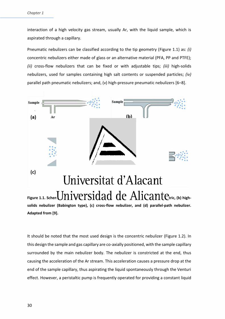
Chapter 1
30
interaction of a high velocity gas stream, usually Ar, with the liquid sample, which is
aspirated through a capillary.
Pneumatic nebulizers can be classified according to the tip geometry (Figure 1.1) as: (i)
concentric nebulizers either made of glass or an alternative material (PFA, PP and PTFE);
(ii) cross-flow nebulizers that can be fixed or with adjustable tips; (iii) high-solids
nebulizers, used for samples containing high salt contents or suspended particles; (iv)
parallel path pneumatic nebulizers; and, (v) high-pressure pneumatic nebulizers [6–8].
Figure 1.1. Schemes of the most used pneumatic nebulization devices. (a) Concentric, (b) high-
solids nebulizer (Babington type), (c) cross-flow nebulizer, and (d) parallel-path nebulizer.
Adapted from [9].
It should be noted that the most used design is the concentric nebulizer (Figure 1.2). In
this design the sample and gas capillary are co-axially positioned, with the sample capillary
surrounded by the main nebulizer body. The nebulizer is constricted at the end, thus
causing the acceleration of the Ar stream. This acceleration causes a pressure drop at the
end of the sample capillary, thus aspirating the liquid spontaneously through the Venturi
effect. However, a peristaltic pump is frequently operated for providing a constant liquid
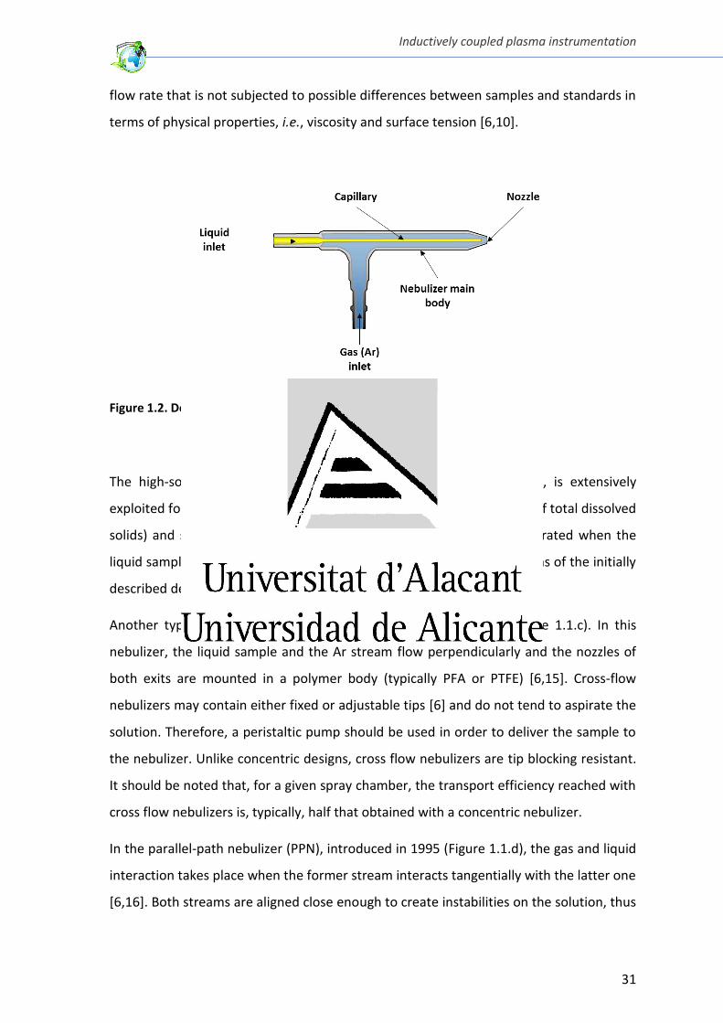
Inductively coupled plasma instrumentation
31
flow rate that is not subjected to possible differences between samples and standards in
terms of physical properties, i.e., viscosity and surface tension [6,10].
Figure 1.2. Detailed scheme of a concentric nebulizer.
The high-solids nebulizer, developed by Babington in 1969 [6,11,12], is extensively
exploited for the analysis of high salt content solutions (e.g., up to 20% of total dissolved
solids) and slurries. In this nebulizer (Figure 1.1.b), the aerosol is generated when the
liquid sample reaches the orifice for the gas stream. Several modifications of the initially
described design, have been reported [13,14].
Another type of nebulizer widely used is the cross-flow design (Figure 1.1.c). In this
nebulizer, the liquid sample and the Ar stream flow perpendicularly and the nozzles of
both exits are mounted in a polymer body (typically PFA or PTFE) [6,15]. Cross-flow
nebulizers may contain either fixed or adjustable tips [6] and do not tend to aspirate the
solution. Therefore, a peristaltic pump should be used in order to deliver the sample to
the nebulizer. Unlike concentric designs, cross flow nebulizers are tip blocking resistant.
It should be noted that, for a given spray chamber, the transport efficiency reached with
cross flow nebulizers is, typically, half that obtained with a concentric nebulizer.
In the parallel-path nebulizer (PPN), introduced in 1995 (Figure 1.1.d), the gas and liquid
interaction takes place when the former stream interacts tangentially with the latter one
[6,16]. Both streams are aligned close enough to create instabilities on the solution, thus
Chapter 1
32
forming the aerosol. The liquid exit is not constrained, being possible the use of larger
orifices than in the nebulizers previously mentioned. As a result, with the PPN, solutions
containing particles and dissolved salts can be easily analyzed. In fact, some of these
nebulizers are provided with liquid capillaries that allow the introduction of slurries
containing particles with diameters of up to about 100 µm.
In the present PhD, concentric and microconcentric nebulizers made in glass and PFA,
respectively, have been used in combination with different spray chambers (see sections
1.1.2 and 1.1.3). Three concentric nebulizers have been used: (i) a nebulizer Meinhard®
type C-0.5 made in glass (Meinhard, Santa Ana, CA, USA) in combination with a total
sample consumption system so-called hTISIS (see section 1.1.3.2) were used in chapters
3 and 4 for the elemental analysis of bioethanol; (ii) a micronebulizer MicroMist® (Glass
Expansion, Melbourne, Australia) coupled to a double pass spray chamber was used for
the analysis of samples coming from different points of the bioethanol production
process, described in chapter 5; and (iii) a PFA-ST micronebulizer (Elemental Scientific,
Omaha, NE, USA) was used in combination with the hTISIS to perform the isotopic analysis
of bioethanol samples (chapter 6).
1.1.2 Spray chambers
Aerosols generated by the nebulizer have characteristics and properties that make
impossible their direct introduction into the plasma. In general terms, the aerosol droplets
reaching the plasma should be small enough (diameter 10 µm) to enable the efficient
desolvation, atomization and ionization of the analytes. Unfortunately, primary aerosols
are normally polydisperse and coarse (with droplets whose diameters range from tens of
nanometers to 100 µm). Therefore, an extra component for adapting the aerosol
properties to the plasma requirements is needed. For this purpose, the nebulizer is,
typically, fitted to a spray chamber. As a result, the aerosol that reaches the plasma
(tertiary aerosol) is monodisperse and fine (see Figure 1.3). Unfortunately, most of the
droplets generated by the nebulizer do not reach the plasma. In fact, for conventional
flow rates (i.e., order of 1 mL min-1) around 95-99.5% of the solution mass aspirated by
the nebulizer is lost in the spray chamber. The main aerosol transport phenomena that
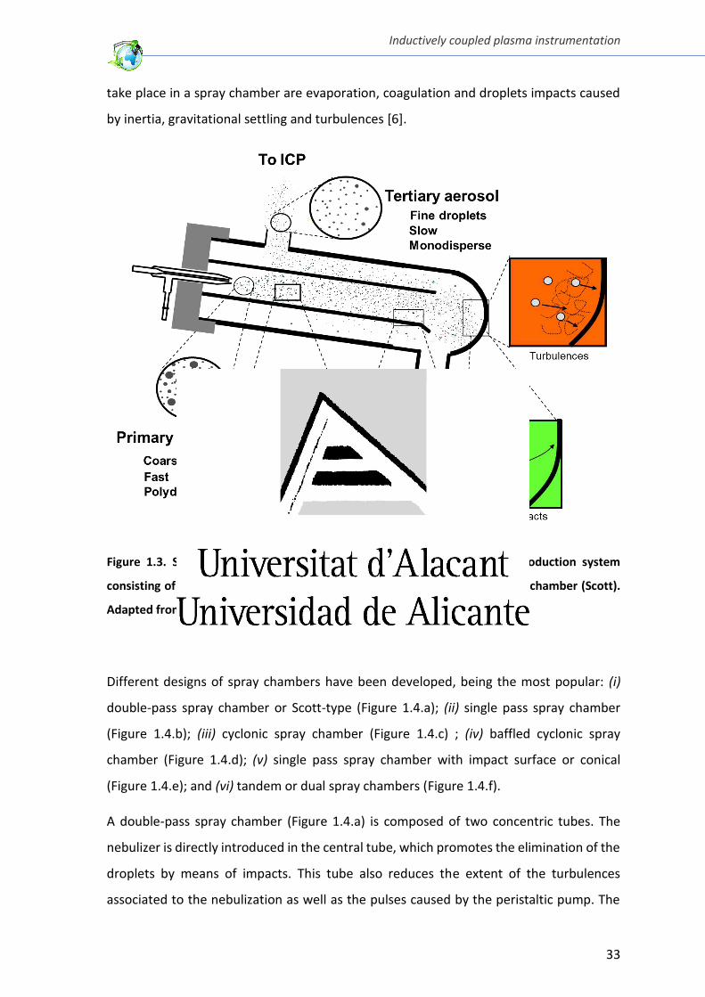
Inductively coupled plasma instrumentation
33
take place in a spray chamber are evaporation, coagulation and droplets impacts caused
by inertia, gravitational settling and turbulences [6].
Figure 1.3. Scheme of the aerosol transport phenomena in a sample introduction system
consisting of a concentric nebulizer in combination with a double-pass spray chamber (Scott).
Adapted from [6].
Different designs of spray chambers have been developed, being the most popular: (i)
double-pass spray chamber or Scott-type (Figure 1.4.a); (ii) single pass spray chamber
(Figure 1.4.b); (iii) cyclonic spray chamber (Figure 1.4.c) ; (iv) baffled cyclonic spray
chamber (Figure 1.4.d); (v) single pass spray chamber with impact surface or conical
(Figure 1.4.e); and (vi) tandem or dual spray chambers (Figure 1.4.f).
A double-pass spray chamber (Figure 1.4.a) is composed of two concentric tubes. The
nebulizer is directly introduced in the central tube, which promotes the elimination of the
droplets by means of impacts. This tube also reduces the extent of the turbulences
associated to the nebulization as well as the pulses caused by the peristaltic pump. The
Chapter 1
34
inner tube also isolates the aerosol passing through the volume left between the internal
and external tubes from the turbulences generated in the nebulization process [6].
Single pass spray chamber (Figure 1.4.b) is a simple device where the nebulizer is coupled
to a single tube or a conical conduction and the aerosol describes a direct trajectory to
the ICP. This design provides the highest transport efficiency, but the median diameter of
the tertiary aerosol is also higher than that obtained with other spray chambers. This
chamber configuration is often used in combination with high efficiency nebulizers or
ultrasonic nebulizers (USN). Single pass spray chambers can be equipped with an impact
surface (Figure 1.4.c) in order to remove the coarsest aerosol droplets [6,17]. As a result,
the aerosol leaving this system is less dispersed and finer than the obtained with no
impact surface, although a higher fraction of the solution is lost and does not escape the
chamber.
Cyclonic spray chambers used in ICP have two main configurations: (i) single-pass cyclonic
spray chamber (Figure 1.4.d) and double-pass cyclonic spray chamber (baffled cyclonic
spray chamber) (Figure 1.4.e). The nebulizer is introduced into the spray chamber
tangentially to the cylindrical body and the tertiary aerosol leaves the chamber through a
tube at the top of the chamber, whereas drains leave the chamber at the bottom.
Therefore, the aerosol first impacts against the chamber walls to be subsequently
transported towards the injector [6].
Additionally, in the last two decades, low inner volume spray chambers have appeared in
order to perform the analysis of microsamples or to improve the transport efficiency for
specific applications. Generally, these chambers are used in combination with a
micronebulizer. The most commonly used low inner volume spray chambers are the
cyclonic (cinnabar) and single-pass designs.
The combination of two spray chambers placed in series has been evaluated for its
application in ICP-MS and MC-ICP-MS. Figure 1.4.f shows a scheme of the most used dual
spray chamber. It contains a cyclonic spray chamber coupled to a double-pass one
[6,18,19]. In this design, the aerosol leaving the cyclonic spray chamber is driven to the
double-pass spray chamber, also called homogenization chamber, before reaching the
plasma. A sensitivity enhancement has been reported when using the dual spray chamber
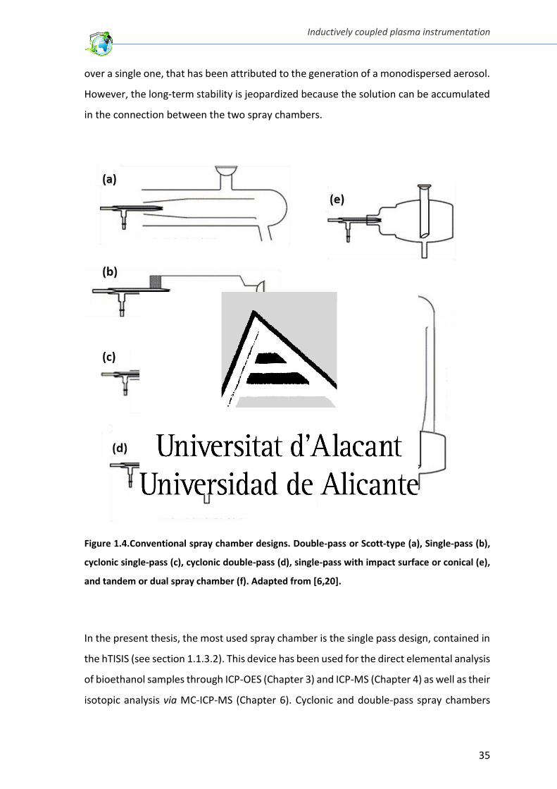
Inductively coupled plasma instrumentation
35
over a single one, that has been attributed to the generation of a monodispersed aerosol.
However, the long-term stability is jeopardized because the solution can be accumulated
in the connection between the two spray chambers.
Figure 1.4.Conventional spray chamber designs. Double-pass or Scott-type (a), Single-pass (b),
cyclonic single-pass (c), cyclonic double-pass (d), single-pass with impact surface or conical (e),
and tandem or dual spray chamber (f). Adapted from [6,20].
In the present thesis, the most used spray chamber is the single pass design, contained in
the hTISIS (see section 1.1.3.2). This device has been used for the direct elemental analysis
of bioethanol samples through ICP-OES (Chapter 3) and ICP-MS (Chapter 4) as well as their
isotopic analysis via MC-ICP-MS (Chapter 6). Cyclonic and double-pass spray chambers
Chapter 1
36
have been used as reference sample introduction systems in the cited chapters. The
double-pass spray chamber has also been applied to the analysis of samples taken along
the bioethanol production process, from the raw material to the final product (Chapter
5). Finally, the dual spray chamber has been used for the lead isotopic characterization of
in-house standards by means of MC-ICP-MS (Chapter 6).
1.1.3 Special sample introduction systems
1.1.3.1 Desolvation systems
The use of desolvation systems has been widely explored due to: (i) the low tolerance of
the plasma to solvent load (especially organic solvents), and (ii) the growing interest of
removing the interferences caused by the solvent. Lowering of the solvent plasma load
can be achieved by working at low liquid flow rates thus reducing the total amount of
aerosol, on the one hand, or removing a significant part of the solvent after the aerosol
formation, on the other hand.
A desolvation system consists of an aerosol heating unit to promote the evaporation of
the solvent contained in the primary aerosol followed by either a condenser or a
membrane (or both) to remove the generated solvent vapor. Under these conditions, the
solvent plasma load decreases and the analyte mass transport rate increases over a
conventional spray chamber thus leading to a sensitivity enhancement.
Figure 1.5. shows a schematic description of two desolvation systems used in ICP-MS and
MC-ICP-MS. The so-called Aridus II (Teledyne Cetac Technologies, NE, USA), Figure 1.5.a,
is equipped with a fluoropolymer evaporation chamber generally used at 110°C and a
membrane, also made in fluoropolymer, operated at 160°C. Figure 1.5.b. shows an outline
of the APEX IR (Elemental Scientific, NE, USA). This desolvation system combines a heated
cyclonic spray chamber (100°C or 140°C) with a multi-pass condenser (-5°C or 2°C). It
should be noted that, if required, a membrane could be adapted to the APEX IR system.
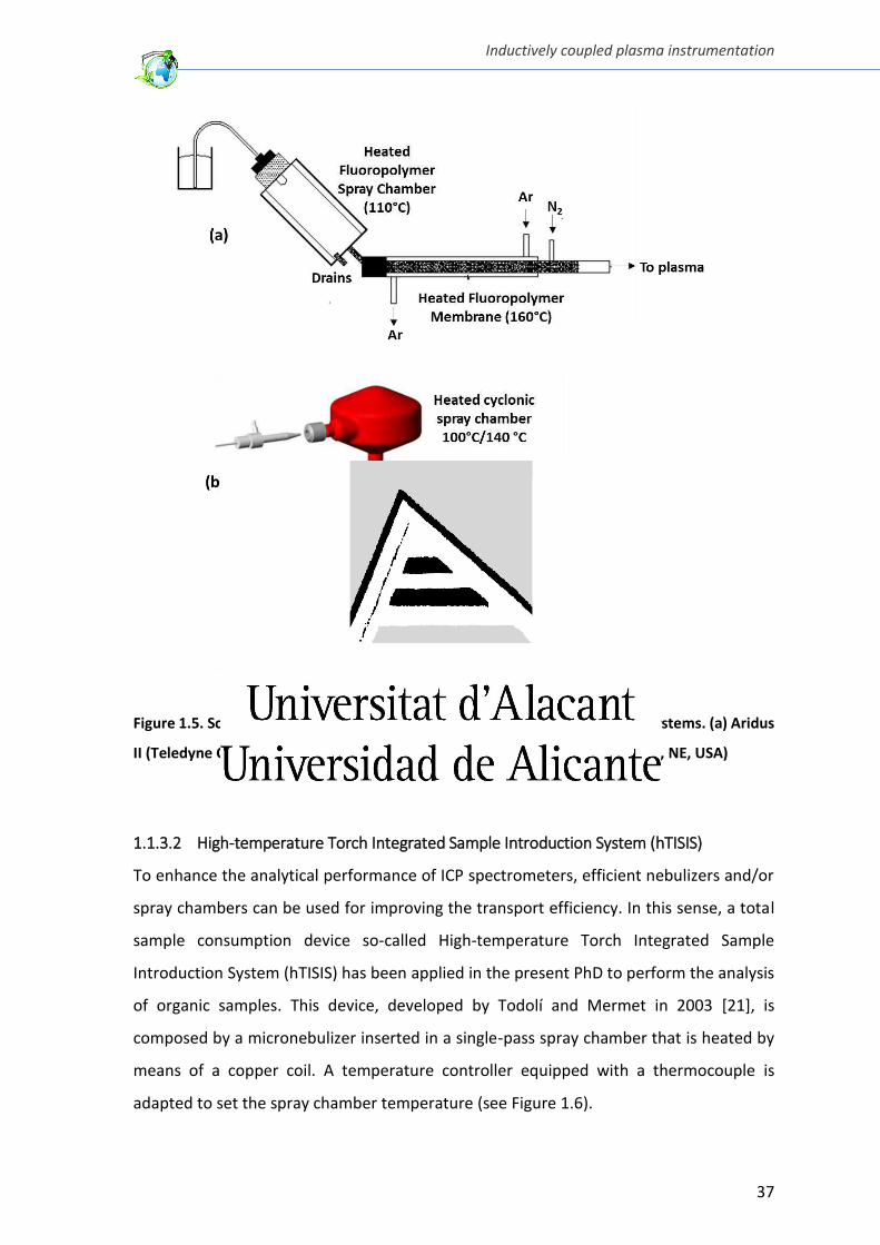
Inductively coupled plasma instrumentation
37
Figure 1.5. Schematic description of two commercially available desolvation systems. (a) Aridus
II (Teledyne Cetac technologies, NE, USA) and (b) APEX IR (Elemental Scientific, NE, USA)
1.1.3.2 High-temperature Torch Integrated Sample Introduction System (hTISIS)
To enhance the analytical performance of ICP spectrometers, efficient nebulizers and/or
spray chambers can be used for improving the transport efficiency. In this sense, a total
sample consumption device so-called High-temperature Torch Integrated Sample
Introduction System (hTISIS) has been applied in the present PhD to perform the analysis
of organic samples. This device, developed by Todolí and Mermet in 2003 [21], is
composed by a micronebulizer inserted in a single-pass spray chamber that is heated by
means of a copper coil. A temperature controller equipped with a thermocouple is
adapted to set the spray chamber temperature (see Figure 1.6).
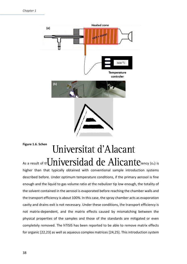
Chapter 1
38
Figure 1.6. Scheme (a) and picture (b) of the hTISIS sample introduction system.
As a result of the heating of the primary aerosol, the analyte transport efficiency (εn) is
higher than that typically obtained with conventional sample introduction systems
described before. Under optimum temperature conditions, if the primary aerosol is fine
enough and the liquid to gas volume ratio at the nebulizer tip low enough, the totality of
the solvent contained in the aerosol is evaporated before reaching the chamber walls and
the transport efficiency is about 100%. In this case, the spray chamber acts as evaporation
cavity and drains exit is not necessary. Under these conditions, the transport efficiency is
not matrix-dependent, and the matrix effects caused by mismatching between the
physical properties of the samples and those of the standards are mitigated or even
completely removed. The hTISIS has been reported to be able to remove matrix effects
for organic [22,23] as well as aqueous complex matrices [24,25]. This introduction system
Inductively coupled plasma instrumentation
39
can be operated in two different flow regimes: (i) continuous sample aspiration mode
(CSA-hTISIS), with liquid flow rates about 30 µL min-1; and (ii) air-segmented injection (ASI-
hTISIS) in which discrete volumes (typically 5 µL) are aspirated using air as carrier. This
second injection mode appeared to solve problems related to the plasma thermal
degradation and the formation of carbon deposits in the ICP-MS interface cones when
organic matrices are introduced into the plasma without using an extra stream of O2.
Additionally, the hTISIS provides other advantages over default setups such as: (i)
sensitivity improvement close to one order of magnitude; (ii) 4- to 5- fold decrease in
limits of detection; (iii) 30-fold shortening of wash-out time because the spray chamber
walls remain dry [6]; (iv) suitability for the analysis of clinical [26,27] or environmental
microsamples [28,29].
In a recent study, the analytical performances obtained with the hTISIS were compared
against those found with an APEX desolvation system, both coupled to ICP-MS. Similar
detection limits and sensitivities were obtained in CSA mode for the APEX and hTISIS
whereas the LODs were about 12 times lower for the latter system in the ASI mode.
Additionally, the matrix effects for aqueous and hydro-organic matrices were less severe
when the hTISIS was operated than when an APEX was used [30].
In the present PhD, the hTISIS has been applied to the direct elemental analysis
(determination of metals) of bioethanol samples in ICP-OES (Chapter 3) and ICP-MS
(Chapter 4) as well as the direct (without sample preparation and/or analyte isolation) Pb
isotopic analysis of bioethanol samples by means of MC-ICP-MS (Chapter 6).
1.2 Plasma source
A plasma is defined as a gas at high temperature that contains molecules, atoms, ions and
electrons. The plasma is generated at the top of a torch normally made in quartz,
consisting of three separated concentric tubes (Figure 1.7). The tertiary aerosol flows
through the central tube or injector. This Ar flow (central flow) ranges from 0.1 to 2 L min-
1. An auxiliary argon stream flows through the space left between the two innermost
tubes. This stream (< 2 L min–1) is used to control the plasma vertical position. Finally, an
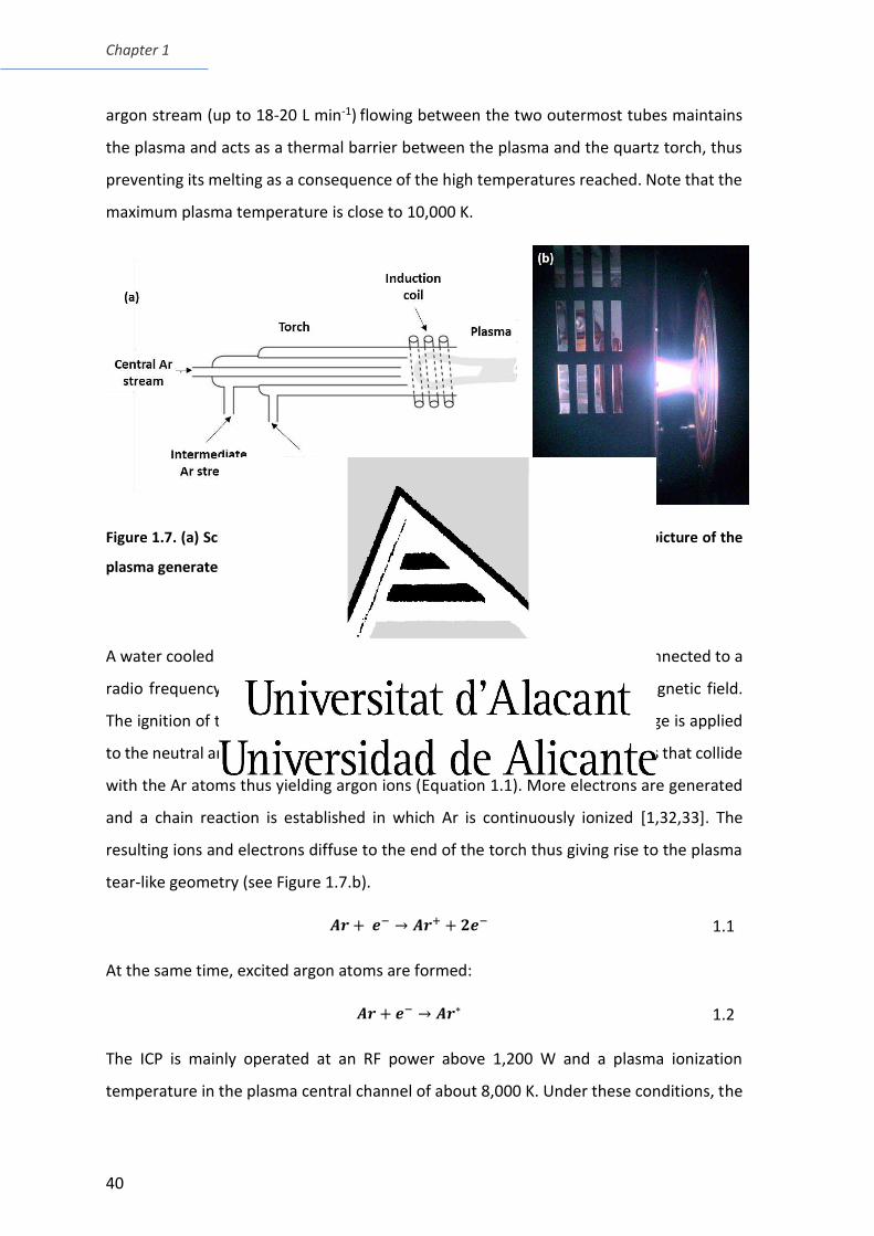
Chapter 1
40
argon stream (up to 18-20 L min-1) flowing between the two outermost tubes maintains
the plasma and acts as a thermal barrier between the plasma and the quartz torch, thus
preventing its melting as a consequence of the high temperatures reached. Note that the
maximum plasma temperature is close to 10,000 K.
Figure 1.7. (a) Scheme the of torch, coil and plasma (Adapted from [31]) and (b) picture of the
plasma generated in an ICP-MS Agilent 7700x spectrometer.
A water cooled copper coil located at the top of the torch (Figure 1.7.a) is connected to a
radio frequency (RF) generator, that produces an intense time-variable magnetic field.
The ignition of the plasma begins when a high-voltage spark or tesla discharge is applied
to the neutral argon gas. The oscillating field accelerates the charged particles that collide
with the Ar atoms thus yielding argon ions (Equation 1.1). More electrons are generated
and a chain reaction is established in which Ar is continuously ionized [1,32,33]. The
resulting ions and electrons diffuse to the end of the torch thus giving rise to the plasma
tear-like geometry (see Figure 1.7.b).
+ − → + + − 1.1
At the same time, excited argon atoms are formed:
+ − → ∗ 1.2
The ICP is mainly operated at an RF power above 1,200 W and a plasma ionization
temperature in the plasma central channel of about 8,000 K. Under these conditions, the
Inductively coupled plasma instrumentation
41
tertiary aerosol leaving the introduction system (see section 1.1) reaches the plasma and
droplets are desolvated, the resulting solid particle is vaporized and the analyte is
successively atomized and excited according to [32]:
� + − → �∗ + − 1.3
After the atomization/excitation process, the ionization takes place by means of: (i)
electron impact (equation 1.4); (ii) charge transfer reactions between ions and atoms
(equation 1.5); and, (iii) penning ionization, caused by collision between atoms and
excited Ar atoms (equation 1.6) [32].
� + − → �+ + − 1.4
� + + → �+ + 1.5
� + ∗ → �+ + + − 1.6
The analyte ionization efficiency α depends on its first ionization potential (Ei). Under the
ICP operating conditions, the ionization efficiency is about 100% for elements with Ei
below 8 eV, between 30 and 80% for metalloids, and from 1 to 30% for non-metals [33].
In addition, excited ions are formed (equations 1.7 - 1.8) [32].
� + ∗ → �+∗ + + − 1.7
� + + → �+∗ + 1.8
Excited analyte atoms can also be generated from ions (Equation 1.9)
�+ + − → �∗ 1.9
1.3 ICP-OES Perkin Elmer Optima 4300DV.
In order to obtain the ICP-OES analytical signal, the radiation emitted from an element at
a given wavelength is isolated from that emitted by other elements or molecules and its
intensity is finally detected [34–36].
An ICP-OES PerkinElmer Optima 4300DV (PerkinElmer, Uberlingen, Germany) instrument
(Figure 1.8) has been used in the present PhD (Chapter 3). The conventional introduction
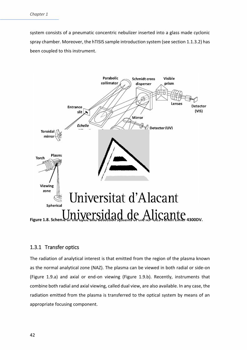
Chapter 1
42
system consists of a pneumatic concentric nebulizer inserted into a glass made cyclonic
spray chamber. Moreover, the hTISIS sample introduction system (see section 1.1.3.2) has
been coupled to this instrument.
Figure 1.8. Scheme of the optic and detection systems of the ICP-OES Perkin Elmer 4300DV.
1.3.1 Transfer optics
The radiation of analytical interest is that emitted from the region of the plasma known
as the normal analytical zone (NAZ). The plasma can be viewed in both radial or side-on
(Figure 1.9.a) and axial or end-on viewing (Figure 1.9.b). Recently, instruments that
combine both radial and axial viewing, called dual view, are also available. In any case, the
radiation emitted from the plasma is transferred to the optical system by means of an
appropriate focusing component.
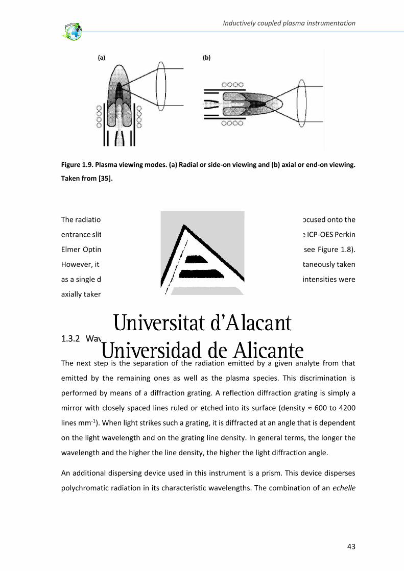
Inductively coupled plasma instrumentation
43
Figure 1.9. Plasma viewing modes. (a) Radial or side-on viewing and (b) axial or end-on viewing.
Taken from [35].
The radiation is collected by a toroidal mirror and image of the plasma is focused onto the
entrance slit of the wavelength dispersing device or spectrometer [35]. The ICP-OES Perkin
Elmer Optima 4300DV instrument incorporates the dual viewing mode (see Figure 1.8).
However, it should be noted that radial and axial intensities are not simultaneously taken
as a single dispersive system is used (Figure 1.8). In the present PhD, the intensities were
axially taken for the analysis of bioethanol samples.
1.3.2 Wavelength dispersive device
The next step is the separation of the radiation emitted by a given analyte from that
emitted by the remaining ones as well as the plasma species. This discrimination is
performed by means of a diffraction grating. A reflection diffraction grating is simply a
mirror with closely spaced lines ruled or etched into its surface (density ≈ 600 to 4200
lines mm-1). When light strikes such a grating, it is diffracted at an angle that is dependent
on the light wavelength and on the grating line density. In general terms, the longer the
wavelength and the higher the line density, the higher the light diffraction angle.
An additional dispersing device used in this instrument is a prism. This device disperses
polychromatic radiation in its characteristic wavelengths. The combination of an echelle
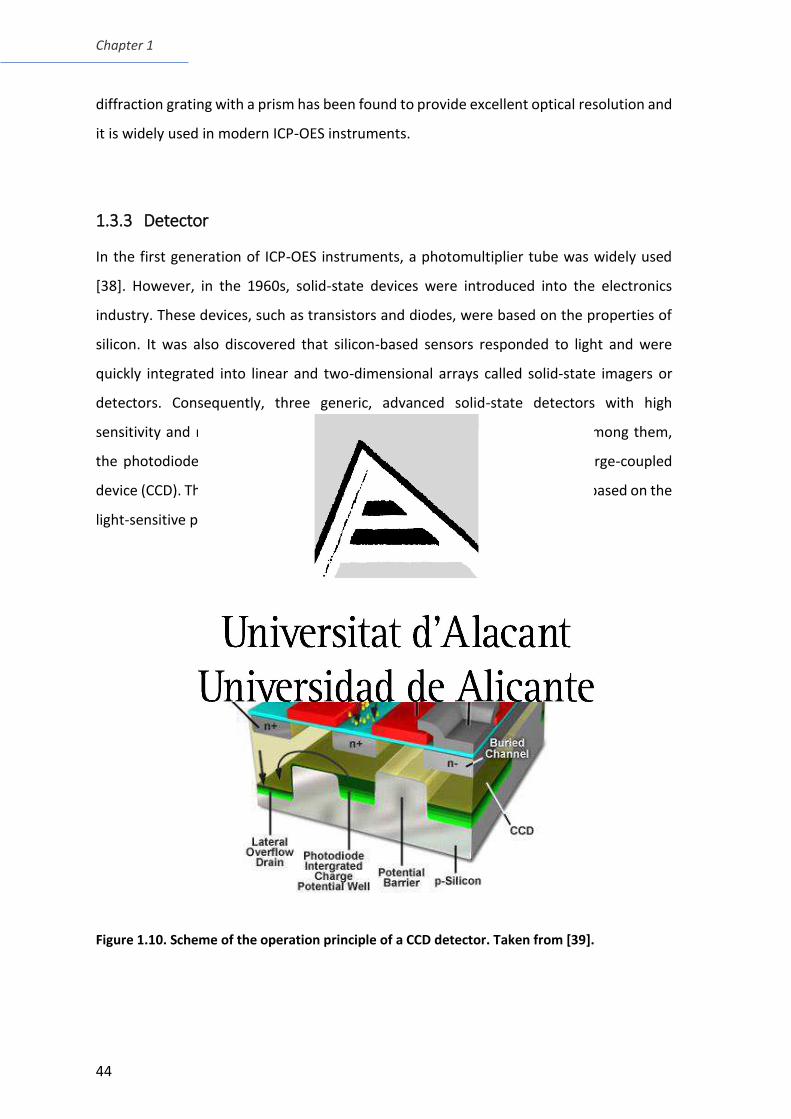
Chapter 1
44
diffraction grating with a prism has been found to provide excellent optical resolution and
it is widely used in modern ICP-OES instruments.
1.3.3 Detector
In the first generation of ICP-OES instruments, a photomultiplier tube was widely used
[38]. However, in the 1960s, solid-state devices were introduced into the electronics
industry. These devices, such as transistors and diodes, were based on the properties of
silicon. It was also discovered that silicon-based sensors responded to light and were
quickly integrated into linear and two-dimensional arrays called solid-state imagers or
detectors. Consequently, three generic, advanced solid-state detectors with high
sensitivity and resolution for spectroscopic applications were developed, among them,
the photodiode array (PDA), the charge-injection device (CID) and the charge-coupled
device (CCD). The CID and CCD devices, or charge-transfer devices (CTD), are based on the
light-sensitive properties of solid-state silicon (Figure 1.10.b) [35,36].
Figure 1.10. Scheme of the operation principle of a CCD detector. Taken from [39].
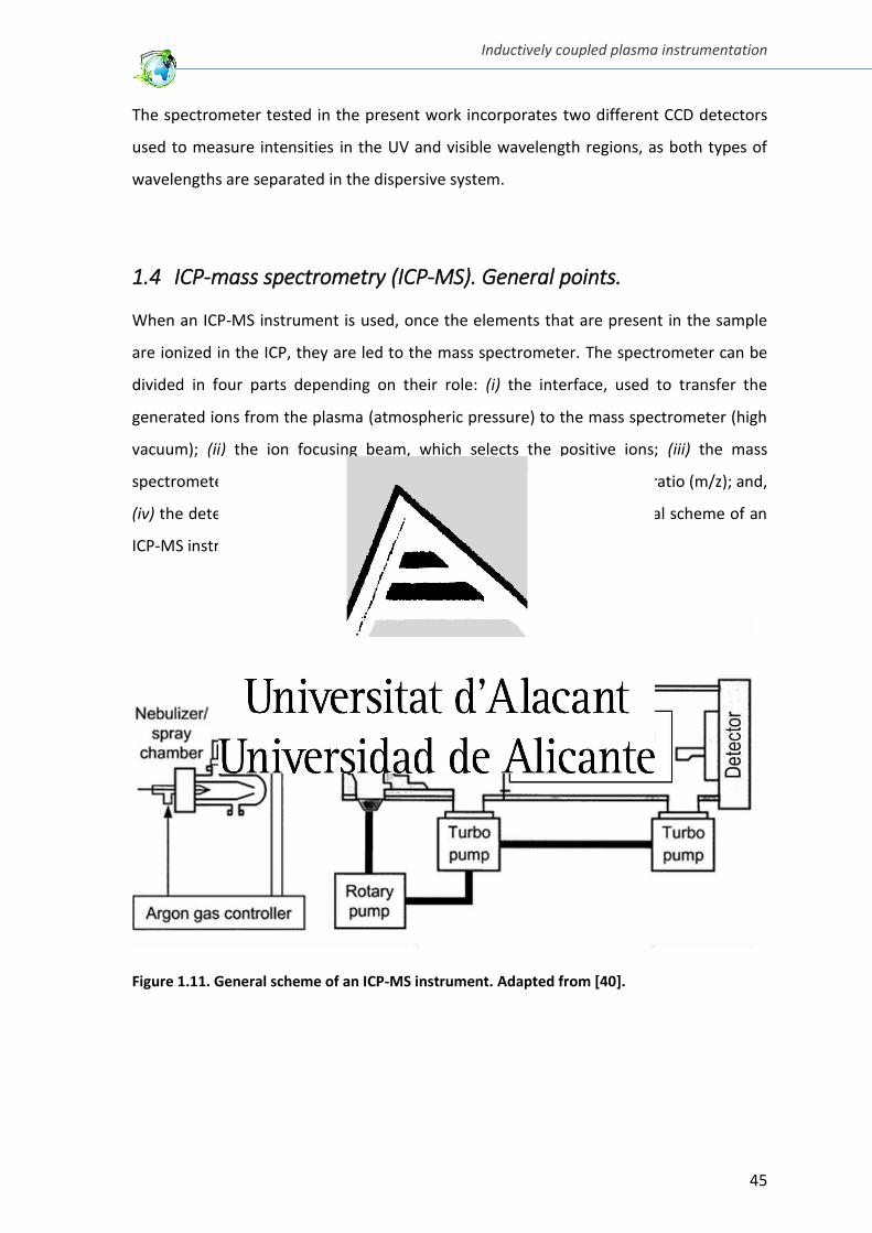
Inductively coupled plasma instrumentation
45
The spectrometer tested in the present work incorporates two different CCD detectors
used to measure intensities in the UV and visible wavelength regions, as both types of
wavelengths are separated in the dispersive system.
1.4 ICP-mass spectrometry (ICP-MS). General points.
When an ICP-MS instrument is used, once the elements that are present in the sample
are ionized in the ICP, they are led to the mass spectrometer. The spectrometer can be
divided in four parts depending on their role: (i) the interface, used to transfer the
generated ions from the plasma (atmospheric pressure) to the mass spectrometer (high
vacuum); (ii) the ion focusing beam, which selects the positive ions; (iii) the mass
spectrometer, that separates the ions according to their mass-to-charge ratio (m/z); and,
(iv) the detector, which is responsible of the signal registration. A general scheme of an
ICP-MS instrument is shown in Figure 1.11
Figure 1.11. General scheme of an ICP-MS instrument. Adapted from [40].
Chapter 1
46
1.4.1 Interface
The ionization process takes place in the plasma at atmospheric pressure whereas the
mass spectrometer operates under high vacuum conditions. For this reason, the interface
plays an important role as the ions need to be efficiently transferred from the plasma to
the mass spectrometer [1]. This interface is generally composed by two co-axial metal
cones with a small central orifice. The first cone is called sampler whereas the second one
is called skimmer (Figure 1.12). These cones are manufactured of an acid-resistant
material with high thermal conductivity, typically Ni or Pt. The latter one, which presents
better properties, is normally used when organic matrices are introduced into the
instrument in combination with an extra oxygen stream.
After the sampler cone, the beam composed by ions, electrons and neutral species
(resulting from the plasma), expands supersonically because of the pressure drop. The
major part of this expanded gas is pumped away by the vacuum pumps. The central part
of the beam is extracted once again by the skimmer.
Figure 1.12. Sampler cone and skimmer. Taken from [41].
1.4.2 Ion focusing system
After the skimmer, the extraction lenses are positioned to select the ions positively
charged, and them are introduced into the ion focusing optics. This part of the instrument
is formed by electrostatic lenses. The ion focusing system can be very simple, being
formed by only one lens, or it can be more complicated combining several lenses.
Inductively coupled plasma instrumentation
47
1.4.3 Mass spectrometer
Once the positive ions are selected in the ion focusing system, they reach the mass
spectrometer. This part of the instrument leads to the separation of the positive ions
based on their mass-to-charge ratio (m/z). Mass spectrometers operate under high
vacuum to avoid collisions between the ions and gas molecules, which would disturb the
ion beam. The characteristics of a mass spectrometer that affect the analytical figures of
merit are resolution, abundance sensitivity and scan speed [8,33].
The mass resolution is defined as the ability of the mass spectrometer to separate two
neighbouring spectral peaks (isotopes). Mass resolution is expressed according to
equation 1.10.
= � 1.10
Where R is the resolution, m the analyte mass and Δm the peak width at 5% of the peak
height corresponding to a given isotope. The resolution necessary to resolve two adjacent
isotope masses can also be calculated by means of equation 1.11:
= +− 1.11
Where m2 and m1 are the masses of both isotopes. In this case, two isotope peaks are
considered to be separated when the valley between the peaks does not exceed 10% of
the peak maximum.
The abundance sensitivity [42] is a parameter that measures the contribution of the tail
of an adjacent peak to the intensity of the analyte. This parameter is calculated as the
ratio between the intensity of the tail at the mass of the analyte and the intensity of the
analyte itself. The abundance sensitivity can be obtained using the peak height or area.
The scan speed is the speed at which the mass spectrometer can scan the spectrum
and/or switch from one mass to another. This characteristic is especially important when
working with either transient signals or isotope ratios.
Chapter 1
48
There are three types of mass spectrometers commercially available: (i) Quadrupole filter
(ICP-QMS), (ii) double-focusing sector field (ICP-SFMS) and (iii) time of flight (ICP-TOF-MS),
that report different resolution and scanning speed (see Table 1.1).
Table 1.1. Comparison of the three types of mass spectrometers used in ICP-MS. Taken from
[33].*
Type of mass
spectrometer Mass resolution
Scanning speed
Speed / u s-1 Full spectrum / ms
Quadrupole filter Unit mass resolution R ≈ 300 2500 100
Sector field Rmax ≈ ,000 1500 150
Time-of-flight Unit mass resolution R ≈ 7500000 0.003
* The operation principle of a quadrupole filter is explained in detail when ICP-QMS is
presented (see section 1.5.2), whereas the double-focusing sector field is explained in the
section where the MC-ICP-MS instrument is described (see section 1.6.1)
1.5 ICP-QMS Agilent 7700x
In the present PhD, most of the experiments carried out in ICP-MS have been performed
by means of an Agilent 7700x instrument (Agilent, Santa Clara, CA, USA). Figure 1.13
shows a detailed scheme of this instrument.
The conventional sample introduction system consists of a micronebulizer micromist®
(Glass Expansion, Melbourne, Australia) inserted in a double pass spray chamber (Scott-
type) made of glass. The hTISIS introduction system (see section 1.1.3.2) has also been
coupled to this instrument for carrying out the quantification of metals in bioethanol
samples (chapter 4). The conventional sample introduction system has been used as a
reference setup to compare the results obtained with the hTISIS and for the elemental
analysis of samples taken in different points of the bioethanol production process
(chapter 5).
Inductively coupled plasma instrumentation
49
Figure 1.13. Detailed scheme of the ICP-MS Agilent 7700x used in chapters 4 and 5. Adapted
from [43].
Chapter 1
50
The ICP-MS Agilent 7700x is equipped with the high matrix introduction (HMI) system.
This device dilutes the tertiary aerosol formed in the spray chamber with an extra argon
stream and it allows the introduction of high salt content and/or hydro-organic matrices
avoiding the formation of deposits of salts and/or carbon in the injector and interface
cones. Obviously, the maximum concentration of organic solvent that can be introduced
into the system depends on the sample flow rate and the ratio nebulizer/HMI gas flows.
The plasma is generated by a frequency-matching 27 MHz generator with 1,600 W
maximum power. The standard interface is composed by Ni-made sampler and skimmer
cones, with orifices of 1.0 mm and 0.4 mm, respectively. The extraction system contains
four different lenses: (i) extraction lens 1, (ii) extraction lens 2, (iii) omega lens, and (iv)
omega bias. Once the ion beam is focused, it reaches the octopole reaction cell (ORC), in
this case designed to be operated in collision mode (KED) using He (described in section
1.5.1) and, after that, the masses are filtered in the quadrupole (section 1.5.2). Finally, the
ions reach the detector, an electron multiplier (section 1.5.3), and the registered signal is
transformed and transferred to the software.
1.5.1 Collision cell.
Spectral interferences are generally classified into three major groups (Table 1.2): isobaric,
multiply (mostly doubly) charged ions, or polyatomic (molecular). Isobaric interferences
occur when nuclides from different elements have the same nominal mass. Doubly
charged ions are formed when an ion is generated with a double positive charge and
produces a spectral peak at half its mass (e.g., 88Sr2+ and 44Ca+). The level of doubly
charged species depends on the ionization conditions that in turn are related with the
nebulizer gas flow, RF power, and torch position [1]. Polyatomic or molecular ions consist
of two or more atoms and typically contain Ar, and/or elements from the sample matrix,
the solvent and/or the surrounding air. Moreover, intense signals of neighbouring ions,
for instance derived from the matrix elements, may overlap with the signal of the target
element.
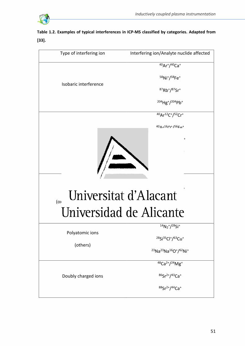
Inductively coupled plasma instrumentation
51
Table 1.2. Examples of typical interferences in ICP-MS classified by categories. Adapted from
[33].
Type of interfering ion Interfering ion/Analyte nuclide affected
Isobaric interference
40Ar+/40Ca+
58Ni+/58Fe+
87Rb+/87Sr+
204Hg+/204Pb+
Polyatomic ions
(Ar-containing)
40Ar12C+/52Cr+
40Ar16O+/56Fe+
40Ar23Na+/63Cu+
40Ar35Cl+/75As+
40Ar2+/80Se+
Polyatomic ions
(oxide and hydroxide ions)
12C16O+/28Si+
12C16O1H+/29Si+
32S16O+/48Ti+
35Cl16O+/51V+
Polyatomic ions
(others)
14N2+/28Si+
28Si35Cl+/63Cu+
23Na23Na16O+/62Ni+
Doubly charged ions
48Ca2+/24Mg+
86Sr2+/43Ca+
88Sr2+/44Ca+
Chapter 1
52
Several strategies have been proposed to overcome spectral interferences, such as
increasing the mass resolution in sector-field instruments, chemical or energy resolution
using a reaction/collision cell (CRC), cold plasma conditions, mathematical corrections,
and chemical separation of the target analyte from the sample matrix [44]. In the present
section, only the use of a CRC is discussed in detail.
The CRC is a universal and flexible strategy to reduce the extent of spectral interferences
in ICP-MS equipped with a quadrupole mass spectrometer. The cell, containing a
multipole under a radio frequency potential, is positioned between the interface and the
mass analyzer and filled with an appropriate gas. The analyte ion can be separated via
selective ion-chemical reactions of the interfering ion with the reaction gas in the cell with
subsequent neutralization or change in its m/z ratio. Newly formed species, as a result of
the reactions, can be eliminated by kinetic energy discrimination using a deceleration
voltage. Alternatively, the target ion can be involved in a selective reaction and measured
as a reaction product ion. Another approach is based on the use of an inert collision gas
(He or H2) in combination with energy discrimination (KED). As a result, a decelerating
voltage may be applied to discriminate selectively against the polyatomic ions [33,45]. The
ICP-QMS used in the present PhD incorporates a collision cell, where He is introduced as
collision gas. As the cross section of the polyatomic ions (interfering ions) is larger than
that for the analyte, the loss of kinetic energy suffered by the polyatomic species is higher
than that suffered by the analyte and, thus, the KED mode is used for discriminating
selectively the ions (Figure 1.14).
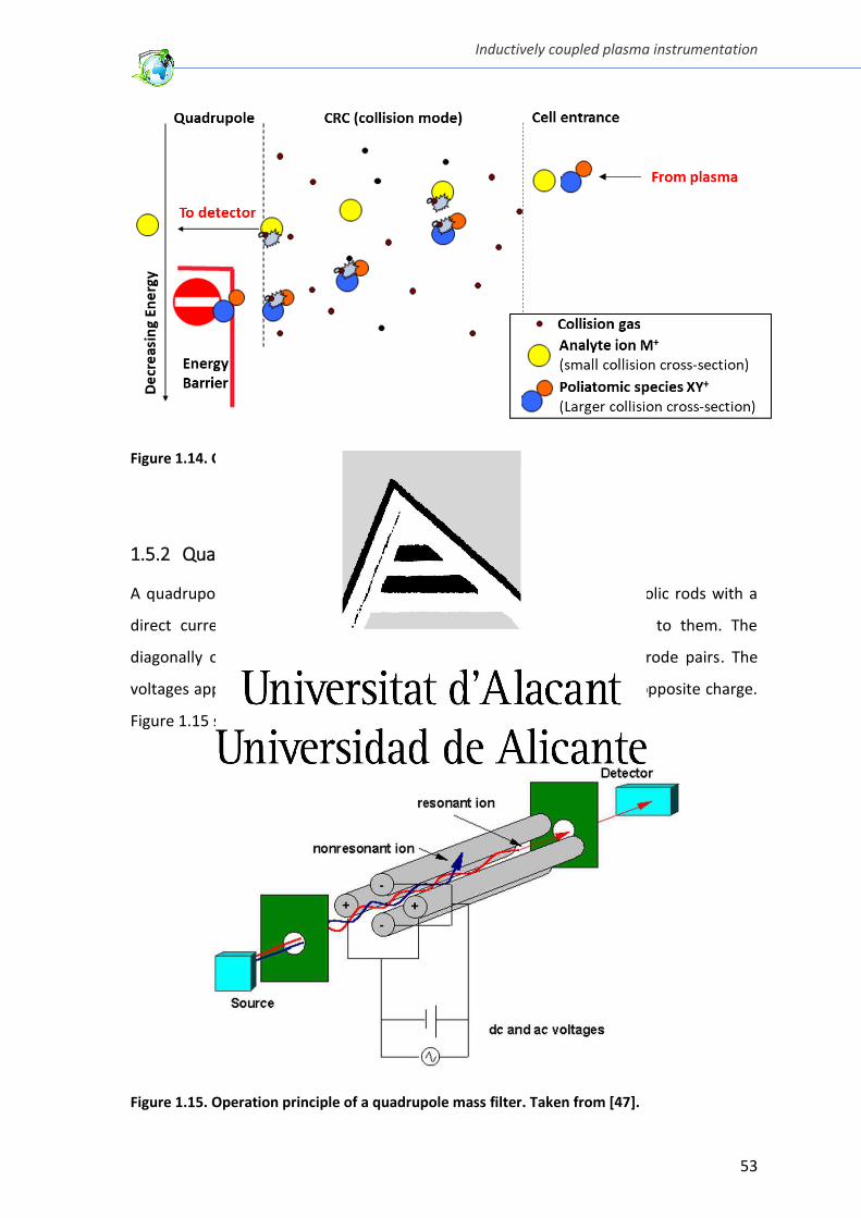
Inductively coupled plasma instrumentation
53
Figure 1.14. Collision-cell operation principle. Adapted from [46].
1.5.2 Quadrupole filter
A quadrupole filter [5,33] consists of four parallel cylindrical or hyperbolic rods with a
direct current (DC) and an alternating current (AC) voltages applied to them. The
diagonally opposed rods are electrically connected, forming two electrode pairs. The
voltages applied on both pairs, have the same magnitude but show an opposite charge.
Figure 1.15 shows the operation principle of the quadrupole filter.
Figure 1.15. Operation principle of a quadrupole mass filter. Taken from [47].
Chapter 1
54
The focused ion beam coming from the ion optics is directed into the quadrupole central
channel. The positive DC component (+U) forces the ions to move towards the axis of the
od a d the AC o po e t Vsi ωt fo uses the io s to the e te du i g the fi st half
period and defocuses the ions from the center in the direction of the rods during the
second half period. Heavy ions are focused on the central axis and lighter ions are
sufficiently accelerated towards the quadrupole rods and removed from the ion beam.
The average potential is positive and this pair of the electrodes acts as a high-mass filter.
The voltage applied to the other pair of electrodes shows the same magnitude with
opposite sign. In this case, the pair of electrodes consist of a DC component (-U) and an
AC component, which shows a phase difference of 180° Vsi ωt + π)). The average
potential is negative and thus, this pair of electrodes acts as a low-mass filter. In this way,
the heavier ions are defocused and removed from the ion beam, while the lighter ions are
focused on the central axis. Thus, the combination of the two electrode pairs results in a
bandpass filter (see Figure 1.16). The DC and AC voltages are selected in such a way that
only the ions within a selected narrow mass-to-charge ratio range can pass through the
quadrupole filter. The dynamic selection of masses passing the filter is accomplished by
changing the DC and AC voltages in such a way that the ratio of their magnitudes remains
constant [32,33,48]. The most notable advantages of the quadrupole mass analyzer are
its technical simplicity with rapid scanning, larger tolerance towards the spread of the
kinetic energies of ions entering the filter, possibility to operate at higher pressure and,
consequently, relatively low cost. The major disadvantage of the quadrupole mass
spectrometer is the low ass esolutio /Δ ≈ .
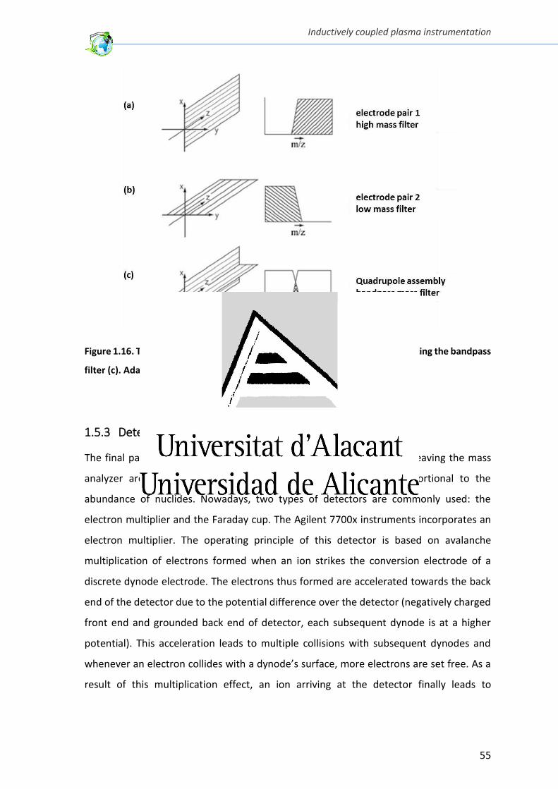
Inductively coupled plasma instrumentation
55
Figure 1.16. The combination of the high-mass (a) and low mass (b) filters resulting the bandpass
filter (c). Adapted from [49].
1.5.3 Detector
The final part of an ICP-MS unit is the ion detection system. The ions leaving the mass
analyzer are detected and transformed into a suitable signal, proportional to the
abundance of nuclides. Nowadays, two types of detectors are commonly used: the
electron multiplier and the Faraday cup. The Agilent 7700x instruments incorporates an
electron multiplier. The operating principle of this detector is based on avalanche
multiplication of electrons formed when an ion strikes the conversion electrode of a
discrete dynode electrode. The electrons thus formed are accelerated towards the back
end of the detector due to the potential difference over the detector (negatively charged
front end and grounded back end of detector, each subsequent dynode is at a higher
potential). This acceleration leads to multiple collisions with subsequent dynodes and
he e e a ele t o ollides ith a dy ode’s su fa e, o e ele t o s a e set f ee. As a
result of this multiplication effect, an ion arriving at the detector finally leads to
Chapter 1
56
approximately 107–108 electrons. Each ion is individually detected in pulse counting mode
[33,50].
1.6 MC-ICP-MS Thermo Neptune.
High-precision isotopic analysis via multi-collector inductively coupled plasma-mass
spectrometry (MC-ICP-MS) instrument is widely used to perform the isotopic analysis of
several types of samples. Modern MC-ICP-MS provide similar precisions to those provided
by thermal ionization mass spectrometry (TIMS) instruments (RSD about 0.002%, under
ideal conditions) [51,52] but with higher sample throughput. Moreover, the ICP is capable
of ionizing elements with high ionization energies as Cu, Fe, W, B, Sb or Hg at atmospheric
pressure.
A MC-ICP-MS Thermo Neptune (Thermo, Bremen, Germany) instrument has been used in
the present PhD, for the determination of lead isotope ratios in bioethanol samples
(chapter 6).
The conventional sample introduction system of this instrument is a PFA micronebulizer
(Elemental Scientific, Omaha, NE, USA) coupled to a dual spray chamber (see section 1.1).
However, the hTISIS sample introduction system (see section 1.1.3.2) as well as a cyclonic
spray chamber, both equipped with an extra gas stream for the addition of oxygen, have
also been adapted to this instrument.
The instrument is equipped with a 130 m3 h-1 dry interface pump and two different types
of interface can be set-up: (i) standard interface and (ii) jet interface. In both cases, the
orifices of both sampler and skimmer are 0.8 mm id. However, the jet interface enhances
the sensitivity from 4 to 50 times due to the differences in terms of geometry between
both interfaces that provide a significantly higher ion extraction efficiency from the
plasma [53,54]. In the work carried out as part of the present PhD, a conventional Pt
sampler cone was combined with two Pt skimmer cones: (i) jet or X-type skimmer, and (ii)
standard skimmer or H-type skimmer.
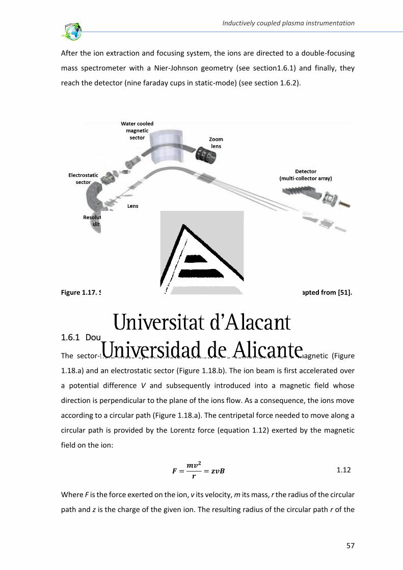
Inductively coupled plasma instrumentation
57
After the ion extraction and focusing system, the ions are directed to a double-focusing
mass spectrometer with a Nier-Johnson geometry (see section1.6.1) and finally, they
reach the detector (nine faraday cups in static-mode) (see section 1.6.2).
Figure 1.17. Scheme of the MC-ICP-MS Thermo Neptune used in chapter 6. Adapted from [51].
1.6.1 Double-focusing mass spectrometer
The sector-field mass spectrometer consists of a combination of a magnetic (Figure
1.18.a) and an electrostatic sector (Figure 1.18.b). The ion beam is first accelerated over
a potential difference V and subsequently introduced into a magnetic field whose
direction is perpendicular to the plane of the ions flow. As a consequence, the ions move
according to a circular path (Figure 1.18.a). The centripetal force needed to move along a
circular path is provided by the Lorentz force (equation 1.12) exerted by the magnetic
field on the ion:
= = 1.12
Where F is the force exerted on the ion, v its velocity, m its mass, r the radius of the circular
path and z is the charge of the given ion. The resulting radius of the circular path r of the
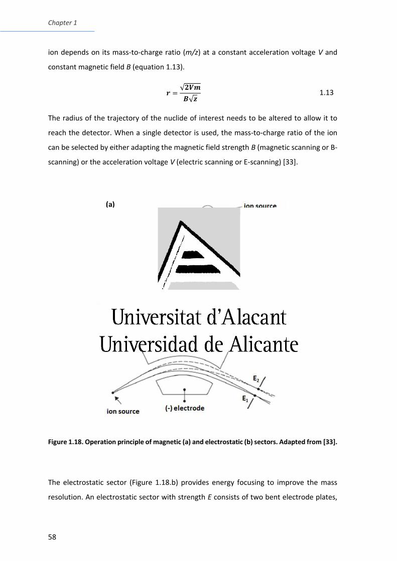
Chapter 1
58
ion depends on its mass-to-charge ratio (m/z) at a constant acceleration voltage V and
constant magnetic field B (equation 1.13).
= √ �√ 1.13
The radius of the trajectory of the nuclide of interest needs to be altered to allow it to
reach the detector. When a single detector is used, the mass-to-charge ratio of the ion
can be selected by either adapting the magnetic field strength B (magnetic scanning or B-
scanning) or the acceleration voltage V (electric scanning or E-scanning) [33].
Figure 1.18. Operation principle of magnetic (a) and electrostatic (b) sectors. Adapted from [33].
The electrostatic sector (Figure 1.18.b) provides energy focusing to improve the mass
resolution. An electrostatic sector with strength E consists of two bent electrode plates,
Inductively coupled plasma instrumentation
59
to which potentials equal in magnitude but opposite in charge are applied. The ions,
moving between the positively and negatively charged bent plate, are forced to move
along a circular path. The centripetal force required to move ions along a circular path, is
provided by the electrostatic force (equation 1.14) [33].
= = 1.14
As a result, the radius of the circular path of an ion depends on its kinetic energy (equation
1.15).
= = 1.15
The combination of magnetic and electrostatic sectors radically improves the mass
resolution, but lowers the transmission efficiency as less ions eventually reach the
detector [32,33,48]. In a double-focusing setup, the electrostatic and magnetic sectors are
combined. Although three different double-focusing geometries (Mattauch-Herzog, Nier-
Johnson and reversed Nier-Johnson geometry) have been reported [33], only the Nier-
Johnson geometry is described in this chapter, since it is the setup incorporated by the
Thermo Neptune MC-ICP-MS instrument. In this geometry (Figure 1.19), the electrostatic
sector is followed by the magnetic sector (both at 90°). Double-focusing is not
simultaneously applied to all the ions, but present-day MC-ICP-MS instruments show a
mass range from m up to 1.3m wherein the ion signals can be monitored under static
conditions (constant magnetic field and acceleration voltage) [33]. Sector-field mass
analyzers are characterized by a high mass resolution (up to 10,000), low abundance
sensitivity, high ion transmission efficiency, and flat-topped peaks with a trapezoidal
shape [33,48].
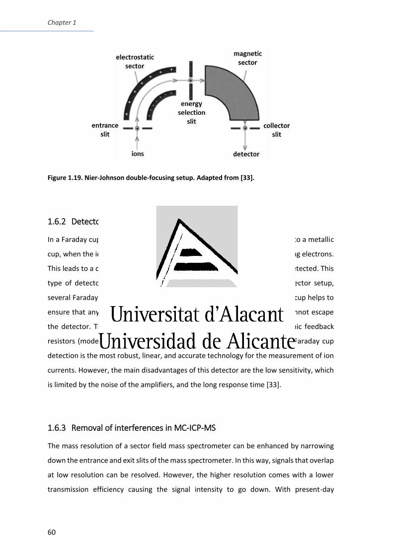
Chapter 1
60
Figure 1.19. Nier-Johnson double-focusing setup. Adapted from [33].
1.6.2 Detector
In a Faraday cup, the ion beam coming from the mass analyzer is directed into a metallic
cup, when the ions reach the wall of the cup, they are neutralized by accepting electrons.
This leads to a current through the resistor, which is further amplified and detected. This
type of detector consists of a thin and deep bucket (cup). In a multi-collector setup,
several Faraday cups are fitted onto movable stages. The large depth of the cup helps to
ensure that any secondary electron produced by energetic incident ions cannot escape
the detector. The cups are connected to current amplifiers with high-ohmic feedback
resistors (modern systems have amplifiers of 1010, 1011,1012, and 1013 Ω . Fa aday up
detection is the most robust, linear, and accurate technology for the measurement of ion
currents. However, the main disadvantages of this detector are the low sensitivity, which
is limited by the noise of the amplifiers, and the long response time [33].
1.6.3 Removal of interferences in MC-ICP-MS
The mass resolution of a sector field mass spectrometer can be enhanced by narrowing
down the entrance and exit slits of the mass spectrometer. In this way, signals that overlap
at low resolution can be resolved. However, the higher resolution comes with a lower
transmission efficiency causing the signal intensity to go down. With present-day
Inductively coupled plasma instrumentation
61
instruments, a mass resolution of 10,000 can be achieved. But for some interferences
even this high mass resolution is not enough to separate the overlapping signals (e.g., 87Sr
and 87Rb).
The Thermo Neptune, used in this work, has three predefined resolution settings: low
esolutio LR, R ≈ , ediu esolutio MR, R ≈ ,000) a d high HR, R ≈ ,000).
When changing from low resolution (LR) to medium resolution (MR) or from medium
resolution to high resolution (HR), the signal intensity goes down by a factor of 10 and 4,
respectively.
Another way to eliminate interferences is the isolation of the target element from the
sample matrix prior the isotopic analysis via MC-ICP-MS. For this purpose, ion exchange
chromatography (off-line with cartridges or columns and on-line chromatographic
methods) is typically used. It should be noted that the isolation can induce mass-
dependent isotope fractionation, but this effect can be avoided if the recovery is
quantitative [55]. Otherwise, the double spike approach is recommended. Another
disadvantage of this methodology is that the chemical separation can generate an
important amount of waste.
1.6.4 Correction for instrumental mass discrimination
Isotope ratio measurements by MC-ICP-MS are affected by instrumental mass
discrimination, principally due to a more efficient transmission of the heavier isotopes of
the target analyte. This phenomenon is mainly associated with the supersonic expansion
of the ion beam in the interface and the space-charge effects (heavy ions having higher
kinetic energy than light ones are preferentially located at the beam centre, because the
electrostatic repulsion causes defocusing of light ions) [56–60]. Therefore, this effect must
be carefully corrected for in order to obtain precise and accurate isotope ratios [51].
Different approaches have been proposed for mass bias correction based on: (i) external
correction using a certified isotopic reference material (certified isotopic composition); (ii)
an internal correction using an internal standard (intra- or inter-elemental); and (iii) a
combination of both external and internal approaches. The external correction is typically
Chapter 1
62
carried out in a sample-standard bracketing (SSB) approach, where the isotope ratio data
obtained for a sample is referred to the ratio obtained for an isotopic standard measured
before and after the sample. The SSB approach has two major assumptions: (i) the mass
discrimination is supposed to be relatively stable as a function of time; and, (ii) the
external standard and samples show an identical mass discrimination behaviour.
Therefore, matrix matching of the samples and standards should be carried out [51],
which in practice is not always possible (e.g., in the case of bioethanol samples, the sample
matrix is unknown) [33]. Internal standardization using a second isotope pair of the same
element (considered invariant in nature, e.g., 88Sr/86Sr) can be used to correct the target
isotope ratio for instrumental mass discrimination (intra-element internal
standardization) [51,61]. This model not only corrects for instrumental mass
discrimination, but also for any natural mass-dependent isotope fractionation of the
target isotope ratio. However, the main limitation of intra-elemental internal
standardization is the number of isotopes required and the limited applicability. Another
approach is based on using an additional element, admixed to the sample as an internal
standard (IS).
Different models overcoming instrumental mass discrimination have been proposed over
the years [42,51,62–64]. The difference between the measured (Rexp) and the true (Rtrue)
isotope ratios is usually expressed by the mass bias correction coefficient, Kij, according
to equation 1.16
= ∙ � 1.16
The mass-bias correction model, firstly described by Russell et al. (equation 1.17) [65] is
the most used model:
= 1.17
where mi and mj are the nuclide masses, and f is fractionation function.
In general, mass-bias correction models express the mass-bias relation between various
isotope pairs of the same (intra-elemental internal standard) or differing (inter-elemental
Inductively coupled plasma instrumentation
63
internal standard) elements. Thus, the two mass-bias correction factors are assumed to
be proportional to the mass ratio of the nuclides, according to equation 1.18.
,� = ( )( ) 1.18
Woodhead suggested to use the best-fitting straight line through data for the target
isotope ratio (fsample) plotted against those for an IS (fIS), calculated according to equation
1.18, to deduce the correction factor [63]. This model was further revised by Baxter et al.
[64] using a linear regression line between ln(Rsample) and ln(RIS) to establish the correlation
between the correction factors for the analyte and the internal standard. Recently,
Devulder et al. proposed a modification of this method (CAIS) [66]. All these methods
provide similar results.
Instrumental mass discrimination can also be corrected for by using the double spike
approach, where a spike enriched in two isotopes and with known isotopic composition
of the target element is added to the sample [33,67]. Therefore, the target element needs
to have at least four isotopes. This method provides accurate and precise isotope ratio
data and allows to correct for sample loss in any sample preparation step, which can lead
to artificial isotope fractionation. However, besides the number of isotopes required, the
double spike technique also has other disadvantages such as the high cost of high-purity
isotopically enriched materials, lack of sensitivity for some isotopes, potential memory
effects and lower sample throughput.
In the chapter 6 of the present PhD, lead (NIST SRM 981) and thallium (NIST SRM 997)
isotopic reference materials from the National Institute for Standards and Technology
(NIST, Gaithersburg, MD, USA), are used for mass bias correction purposes. Sample-
standard bracketing solution prepared in 75% ethanol has been applied for the mass bias
correction of any ethanol : water matrix ranging from 60 to 100% of ethanol without
matrix matching methodology.
Chapter 1
64
1.7 References
[1] R. Thomas, Practical guide to ICP-MS, Marcel Dekker, Inc., New York, 2004.
[2] R.S. Houk, V.A. Fassel, G.D. Flesch, H.J. Svec, A.L. Gray, C.E. Taylor, Inductively
coupled argon plasma as an ion source for mass spectrometric determination of
trace elements, Anal. Chem. 52 (1980) 2283–2289.
[3] U. Voellkopf, M. Paul, E.R. Denoyer, Analysis of solid samples by ICP-mass
spectrometry, Fresenius. J. Anal. Chem. 342 (1992) 917–923.
[4] A. Montaser, Sample introduction in ICP-MS, in: A. Montaser (Ed.), Inductively
Coupled Plasma Mass Spectrom., Wiley-VCH, New York, 1998: pp. 83–264.
[5] R. Tho as, A egi e ’s guide to ICP-MS, Spectrosc. (Santa Monica). 17 (2002) 36–
41.
[6] J.L. Todoli, Mermet, Liquid sample introduction in ICP spectrometry: a practical
guide, First edit, Elsevier B.V., Amsterdam, 2008.
[7] J. Sneddon, Sample Introduction in Atomic Spectroscopy, Elsevier, Amsterdam,
2012.
[8] A. Montaser, Inductively coupled Plasma Mass Spectrometry, Wiley-VCH, New
York, 1998.
[9] Z. Wang, P. Yang, Slurry nebulization in plasmas for analysis of advanced ceramic
materials, J. Anal. At. Spectrom. 29 (2014) 2091–2103.
[10] B.A. Meinhard, D.K. Brown, J.E. Meinhard, The Effect of Nebulizer Structure on
Flame Emission, Appl. Spectrosc. 46 (1992) 1134–1139.
[11] R.S. Babington, A.A. Yetman, Mathod of atomizing liquid in a mono-disperse spray,
US Patent 3421692, 1969.
[12] R.S. Babington, A.A. Yetman, Apparatus for spraying liquids in mono-dispersed
form, US Patent 3421699, 1969.
Inductively coupled plasma instrumentation
65
[13] J.R. Garbarino, H.E. Taylor, A Babington-type Nebulizer for Use in the Analysis of
Natural Water Samples by Inductively Coupled Plasma Spectrometry, Appl.
Spectrosc. 34 (1980) 584–590.
[14] I. Steffan, G. Vujicic, A new nebulizer for inductively coupled plasma analysis of
solutions with high salt content, Spectrochim. Acta Part B At. Spectrosc. 44 (1989)
229–233.
[15] R.N. Kniseley, H. Amenson, C.C. Butler, V.A. Fassel, An Improved Pneumatic
Nebulizer for Use at Low Nebulizing Gas Flows, Appl. Spectrosc. 28 (1974) 285–286.
[16] J.A. Burgener, Parallel path induction pneumatic nebulizer, US Patent 5411208,
1995.
[17] D.W. Hausler, L.T. Taylor, Nonaqueous on-line simultaneous determination of
metals by size exclusion chromatography with inductively coupled plasma atomic
emission spectrometric detection, Anal. Chem. 53 (1981) 1223–1227.
[18] M. Hamester, D. Wiederin, J. Wills, W. Kerl, C.B. Douthitt, Strategies for isotope
ratio measurements with a double focusing sector field ICP-MS, Fresenius. J. Anal.
Chem. 364 (1999) 495–498.
[19] Y. Anoshkina, M. Costas-Rodríguez, F. Vanhaecke, Iron isotopic analysis of finger-
prick and venous blood by multi-collector inductively coupled plasma-mass
spectrometry after volumetric absorptive microsampling, J. Anal. At. Spectrom. 32
(2017) 314–321.
[20] J.L. Todolí, J.M. Mermet, Sample introduction systems for the analysis of liquid
microsamples by ICP-AES and ICP-MS, Spectrochim. Acta Part B At. Spectrosc. 61
(2006) 239–283.
[21] J.L. Todolí, J.M. Mermet, Optimization of the evaporation cavity in a torch
integrated sample introduction system based ICP-AES system. Applications to
matrix and transient effects, analysis of microsamples and analysis of certified solid
samples, J. Anal. At. Spectrom. 18 (2003) 1185–1191.
Chapter 1
66
[22] R. Sanchez, C. Sanchez, J.L. Todoli, C.P. Lienemann, J.M. Mermet, Quantification of
nickel, vanadium and manganese in petroleum products and biofuels through
inductively coupled plasma mass spectrometry equipped with a high temperature
single pass spray chamber, J. Anal. At. Spectrom. 29 (2014) 242–248.
[23] R. Sanchez, J.L. Todoli, C.P. Lienemann, J.M. Mermet, Universal calibration for
metal determination in fuels and biofuels by inductively coupled plasma atomic
emission spectrometry based on segmented flow injection and a 350 °C heated
chamber, J. Anal. At. Spectrom. 27 (2012) 937–945.
[24] F. Ardini, M. Grotti, R. Sánchez, J.L. Todolí, Improving the analytical performances
of ICP-AES by using a high-temperature single-pass spray chamber and segmented-
injections micro-sample introduction for the analysis of environmental samples, J.
Anal. At. Spectrom. 27 (2012) 1400–1404.
[25] C. Lagomarsino, M. Grotti, J.L. Todolí, J.M. Mermet, Study of the absence of
recondensation with low liquid delivery rates by using a cavity sheathing gas in
inductively coupled plasma-atomic emission spectrometry, J. Anal. At. Spectrom.
22 (2007) 523–531.
[26] Á. Cañabate, E. García-Ruiz, M. Resano, J.L. Todolí, Analysis of whole blood by ICP-
MS equipped with a high temperature total sample consumption system, J. Anal.
At. Spectrom. 32 (2017) 78–87.
[27] Á. Cañabate, E. García-Ruiz, M. Resano, J.L. Todolí, Cerebrospinal fluid elemental
analysis by using a total sample consumption system operated at high temperature
adapted to inductively coupled plasma mass spectrometry, J. Anal. At. Spectrom.
32 (2017) 1916–1924.
[28] A. Bazzano, K. Latruwe, M. Grotti, F. Vanhaecke, Lead isotopic analysis of Antarctic
snow using multi-collector ICP-mass spectrometry, J. Anal. At. Spectrom. 30 (2015)
1322–1328.
[29] A. Bazzano, M. Grotti, Determination of lead isotope ratios in environmental
matrices by quadrupole ICP-MS working at low sample consumption rates, J. Anal.
Inductively coupled plasma instrumentation
67
At. Spectrom. 29 (2014) 926–933.
[30] R. Sánchez, Á. Cañabate, C. Bresson, F. Chartier, H. Isnard, S. Maestre, A. Nonell,
J.L. Todolí, Comparison of a high temperature torch integrated sample introduction
system with a desolvation system for the analysis of microsamples through
inductively coupled plasma mass spectrometry, Spectrochim. Acta - Part B At.
Spectrosc. 129 (2017) 28–36.
[31] https://www.medicinescomplete.com/mc/clarke/2010/Clkatomic_absorption_
spectroscopy__inductively_coupled_plasma-mF004_default.png%0A (accessed
February 13, 2018).
[32] J.S. Becker, Inorganic Mass Spectrometry: Principles and Applications, 2007.
[33] F. Vanhaecke, P. Degryse, Isotopic analysis – Fundamentals and applications using
ICP-MS, Wiley-VCH, 2012.
[34] J. Nölte, ICP Emission Spectrometry: A practical guide., Wiley-VCH, 2003.
[35] C.B. Boss, K.J. Fredeen, Concepts, Instrumentation, and Techniques in Inductively
Coupled Plasma Optical Emission Spectrometry, Second Edi, Perkin Elmer
Instruments, 1997.
[36] X. Hou, B.T. Jones, Inductively Coupled Plasma/Optical Emission Spectrometry, in:
R.A. Meyers (Ed.), Encycl. Anal. Chem., John Wiley & Sons Ltd, Chichester, 2000: pp.
9468–9485.
[37] A.A. Gaertner, H.W. Yoon, T.A. Germer, Dispersive Methods, in: Exp. Methods Phys.
Sci., Academic Press, 2014: pp. 67–95.
[38] Molecular Expressions Microscopy Primer: Digital Imaging in Optical Microscopy -
Concepts in Digital Imaging - Photomultiplier Tubes, (n.d.).
https://micro.magnet.fsu.edu/primer/digitalimaging/concepts/photomultipliers.h
tml (accessed February 24, 2018).
[39] ZEISS Microscopy Online Campus | Microscopy Basics | Understanding Digital
Chapter 1
68
Imaging, (n.d.). http://zeiss-campus.magnet.fsu.edu/print/basics/digitalimaging-
print.html (accessed February 24, 2018).
[40] “.“. Ka a ku a ath, K. W o el, K. W o el, C. B’Hy e , J.A. Ca uso, Capilla y
electrophoresis–inductively coupled plasma-mass spectrometry: an attractive
complementary technique for elemental speciation analysis, J. Chromatogr. A. 975
(2002) 245–266.
[41] ICP-MS Cones | Thermo Fisher (all models) | Analytical West, (n.d.).
https://www.analyticalwest.com/products/icp-ms/icp-ms-thermo-
elemental/cones.html (accessed February 24, 2018).
[42] K.G. Heumann, S.M. Gallus, G. Rädlinger, J. Vogl, Precision and accuracy in isotope
ratio measurements by plasma source mass spectrometry, J. Anal. At. Spectrom. 13
(1998) 1001–1008.
[43] ICP-MS Agilent Serie 7700 Extraordinario ICP-MS de 3a generación, (n.d.).
https://www.agilent.com/cs/library/brochures/5990-4025ES.pdf (accessed
February 24, 2018).
[44] T.S. Lum, K. Sze-Yin Leung, Strategies to overcome spectral interference in ICP-MS
detection, J. Anal. At. Spectrom. 31 (2016) 1078–1088.
[45] S.D. Tanner, V.I. Baranov, D.R. Bandura, Reaction cells and collision cells for ICP-
MS: A tutorial review, Spectrochim. Acta - Part B At. Spectrosc. 57 (2002) 1361–
1452.
[46] Crash! Bang! Wallop! How Does an ICP-MS Collision Cell Work? Part 1, (n.d.).
http://analyteguru.com/crash-bang-wallop-how-does-an-icp-ms-collision-cell-
work-part-1/ (accessed February 24, 2018).
[47] CHP - Quadrupole Mass Spectrometry, (n.d.).
http://www.tissuegroup.chem.vt.edu/chem-ed/ms/quadrupo.html (accessed
February 24, 2018).
[48] E. Hoffmann, V. Stroobant, Mass spectrometry: principles and applications, Wiley-
Inductively coupled plasma instrumentation
69
VCH, 2007.
[49] P.E. Miller, M.B. Denton, The quadrupole mass filter: Basic operating concepts, J.
Chem. Educ. 63 (1986) 617–622.
[50] D.W. Koppenaal, C.J. Barinaga, M.B. Denton, R.P. Sperline, G.M. Hieftje, G.D.
Schilling, F.J. Andrade, J.H. Barnes, I. IV, MS Detectors, Anal. Chem. 77 (2005) 418
A-427 A.
[51] L. Yang, Accurate and precise determination of isotopic ratios by MC-ICP-MS: A
review, Mass Spectrom. Rev. 28 (2009) 990–1011.
[52] F. Vanhaecke, L. Balcaen, D. Malinovsky, Use of single-collector and multi-collector
ICP-mass spectrometry for isotopic analysis, J. Anal. At. Spectrom. 24 (2009) 863-
866.
[53] S.M. Chernonozhkin, M. Costas-Rodríguez, P. Claeys, F. Vanhaecke, Evaluation of
the use of cold plasma conditions for Fe isotopic analysis via multi-collector ICP-
mass spectrometry: effect on spectral interferences and instrumental mass
discrimination, J. Anal. At. Spectrom. 32 (2017) 538–547.
[54] K. Newman, Effects of the sampling interface in MC-ICP-MS: Relative elemental
sensitivities and non-linear mass dependent fractionation of Nd isotopes, J. Anal.
At. Spectrom. 27 (2012) 63–70.
[55] C. Maréchal, F. Albarède, Ion-exchange fractionation of copper and zinc isotopes,
Geochim. Cosmochim. Acta. 66 (2002) 1499–1509.
[56] M. Rehkämper, M. Schönbächler, C.H. Stirling, Multiple collector ICP-MS:
Introduction to instrumentation, measurement techniques and analytical
capabilities, Geostand. Newsl. 25 (2001) 23–40.
[57] C.N. Maréchal, P. Télouk, F. Albarède, Precise analysis of copper and zinc isotopic
compositions by plasma-source mass spectrometry, Chem. Geol. 156 (1999) 251–
273.
Chapter 1
70
[58] C.P. Ingle, B.L. Sharp, M.S.A. Horstwood, R.R. Parrish, D.J. Lewis, Instrument
response functions, mass bias and matrix effects in isotope ratio measurements
and semi-quantitative analysis by single and multi-collector ICP-MS, J. Anal. At.
Spectrom. 18 (2003) 219–229.
[59] H. Andrén, I. Rodushkin, A. Stenberg, D. Malinovsky, D.C. Baxter, Sources of mass
bias and isotope ratio variation in multi-collector ICP-MS: optimization of
instrumental parameters based on experimental observations, J. Anal. At.
Spectrom. 19 (2004) 1217–1224.
[60] N. Kivel, I. Günther-Leopold, F. Vanhaecke, D. Günther, Isotope fractionation during
ion beam formation in multi-collector inductively coupled plasma mass
spectrometry, Spectrochim. Acta - Part B At. Spectrosc. 76 (2012) 126–132.
[61] M. Horsky, J. Irrgeher, T. Prohaska, Evaluation strategies and uncertainty
calculation of isotope amount ratios measured by MC ICP-MS on the example of Sr,
Anal. Bioanal. Chem. 408 (2016) 351–367.
[62] J. Meija, L. Yang, R. Sturgeon, Z. Mester, Mass bias fractionation laws for multi-
collector ICPMS: Assumptions and their experimental verification, Anal. Chem. 81
(2009) 6774–6778.
[63] J. Woodhead, A simple method for obtaining highly accurate Pb isotope data by
MC-ICP-MS, J. Anal. At. Spectrom. 17 (2002) 1381–1385.
[64] D.C. Baxter, I. Rodushkin, E. Engström, D. Malinovsky, Revised exponential model
for mass bias correction using an internal standard for isotope abundance ratio
measurements by multi-collector inductively coupled plasma mass spectrometry,
J. Anal. At. Spectrom. 21 (2006) 427–430.
[65] W.A. Russell, D.A. Papanastassiou, T.A. Tombrello, Ca isotope fractionation on the
Earth and other solar system materials, Geochim. Cosmochim. Acta. 42 (1978)
1075–1090.
[66] V. Devulder, L. Lobo, K. Van Hoecke, P. Degryse, F. Vanhaecke, Common analyte
Inductively coupled plasma instrumentation
71
internal standardization as a tool for correction for mass discrimination in multi-
collector inductively coupled plasma-mass spectrometry, Spectrochim. Acta - Part
B At. Spectrosc. 89 (2013) 20–29.
[67] S.J.G. Galer, Optimal double and triple spiking for high precision lead isotopic
measurement, Chem. Geol. 157 (1999) 255–274.


PUBLISHED WORKS /
TRABAJOS PUBLICADOS


CHAPTER 2
2 Metal a d etalloids deter i atio
i iodiesel a d ioetha ol

Metal and metalloid determination in biodiesel and bioethanol
79
R. Sánchez, C. Sánchez, C.P. Lienemann, J.L. Todolí, Metal and metalloid determination in
biodiesel and bioethanol, J. Anal. At. Spectrom. 30 (2015) 64–101.
doi:10.1039/C4JA00202D
Abstract
Biofuels quality control involves the determination of metal and metalloid content. These
species play a very important role because they may modify the efficiency of the biofuel
production as well as the stability of these products. Furthermore, some metals are toxic
and generate environmental concerns whereas others are used as additives. Normally,
products such as biodiesel and bioethanol are mixed with fossil conventional fuels (diesel
and gasoline, respectively). Therefore, metals come from the raw product employed for
iofuel p odu tio seeds, suga s… as ell as from the production and storage process
or even from the added fuels. The determination of the final metal and metalloid
concentration in biofuels is a challenging subject because of several reasons. On the one
hand, their content is usually low (i.e., f o se e al μg L-1 to mg L-1) and, hence, sensitive
techniques should be used. Besides all this, calibration with organic complex matrices
becomes more difficult and degrades the accuracy of the determination. Several
approaches have been evaluated to carry out this kind of analysis going from
spectrochemical to electroanalytical techniques. Within the first group, Inductively
Coupled Plasma Optical Emission Spectroscopy (ICP-OES) and Mass Spectrometry (ICP-
MS) are often employed together with Atomic Absorption methods. The different
procedures applied will be discussed in the present review emphasizing the most widely
employed ones. On this subject, fundamental as well as applied studies related with the
biofuels analysis through ICP-OES and ICP-MS will be shown to illustrate the current
difficulties associated to these determinations. Comments regarding to the possible
solutions proposed to overcome the drawbacks encountered will be made.

CHAPTER 3
3 Metal a d etalloid deter i atio i
ioetha ol through i du ti ely
oupled plas a-opti al e issio
spe tros opy

Metal and metalloid determination in bioethanol through ICP-OES
187
C. Sánchez, C.P. Lienemann, J.L. Todolí, Metal and metalloid determination in bioethanol
through inductively coupled plasma-optical emission spectroscopy, Spectrochim. Acta
Part B At. Spectrosc. 115 (2016) 16–22.
doi:10.1016/j.sab.2015.10.011
Abstract
A new method to carry out the elemental determination of metals in bioethanol through
ICP-OES has been developed. The procedure is based on the use of a heated Torch
Integrated Sample Introduction System (hTISIS) to directly introduce the vaporized sample
into the plasma. Two injection modes, continuous sample aspiration (CSA) and air-
segmented flow injection analysis (ASI), have been evaluated. In a first step, the matrix
effects caused by several ethanol-water mixtures were removed by operating the hTISIS
at 400°C in air-segmented injection. Meanwhile, the results also proved that the system
could be operated in continuous mode at 200°C with the complete interferences removal.
Finally, twenty-eight real samples with bioethanol contents between 55% and 100% were
analyzed with the methods previously developed. Regarding validation, recoveries from
80% to 120% were obtained for 18 analytes and the concentrations found with the
proposed method were in agreement with those encountered with a preconcentration
method, taken as a reference procedure. Limits of detection went from 3 ng mL-1 for
manganese to about 500 ng mL-1 for calcium. This allowed to quantify Cr, Fe, Mg, Mn and
Zn in segmented flow injection and Al, Cd, Cr, Cu, K, Mg, Mn, Na and Zn in continuous
sample aspiration mode in bioethanol samples.

.
CHAPTER 4
4 A alysis of ioetha ol sa ples
through I du ti ely Coupled Plas a-
Mass Spe tro etry ith a total
sa ple o su ptio syste

Analysis of bioethanol samples through ICP-MS using the hTISIS
217
C. Sánchez, C.P. Lienemann, J.L. Todolí, Analysis of bioethanol samples through Inductively
Coupled Plasma Mass Spectrometry with a total sample consumption system,
Spectrochim. Acta - Part B At. Spectrosc. 124 (2016) 99-108.
doi:10.1016/j.sab.2016.08.018.
Abstract
Bioethanol real samples have been directly analyzed through ICP-MS by means of the so
called High Temperature Torch Integrated Sample Introduction System (hTISIS). Because
bioethanol samples may contain water, experiments have been carried out in order to
determine the effect of ethanol concentration on the ICP-MS response. The ethanol
content studied went from 0 to 50%, because higher alcohol concentrations led to carbon
deposits on the ICP-MS interface. The spectrometer default spray chamber (double pass)
equipped with a glass concentric pneumatic micronebulizer has been taken as the
reference system. Two flow regimes have been evaluated: continuous sample aspiration
at 25 L min-1 and 5 L air-segmented sample injection. hTISIS temperature has been
shown to be critical, in fact ICP-MS sensitivity increased with this variable up to 100 – 200
°C depending on the solution tested. Higher chamber temperatures led to either a drop
in signal or a plateau. Compared with the reference system, the hTISIS improved the
sensitivities by a factor included within the 4 to 8 range while average detection limits
were 6 times lower for the latter device. Regarding the influence of the ethanol
concentration on sensitivity, it has been observed that an increase in the temperature was
not enough to eliminate the interferences. It was also necessary to modify the torch
position with respect to the ICP-MS interface to overcome them. This fact was likely due
to the different extent of ion plasma radial diffusion encountered as a function of the
matrix when working at high chamber temperatures. When the torch was moved 1 mm
plasma down axis, ethanolic and aqueous solutions provided statistically equal
sensitivities. A preconcentration procedure has been applied in order to validate the
methodology. It has been found that, under optimum conditions from the point of view
of matrix effects, recoveries for spiked samples were close to 100%. Furthermore,
analytical concentrations for real samples following the preconcentration method and the
Chapter 4
218
direct determination were not significantly different. The quantification method was
finally based on external calibration with standards containing 50% (v/v) ethanol content.
CHAPTER 5
5 E olutio of the etal a d etalloid
o te t alo g the ioetha ol
produ tio pro ess

Evolution of the metal and metalloid content along the bioethanol production process
251
C. Sánchez, J.P. Vidal, C.P. Lienemann, J.L. Todolí, Evolution of the metal and metalloid
content along the bioethanol production process, Fuel Process. Technol. 173 (2018) 1–10.
doi:10.1016/j.fuproc.2018.01.001.
Abstract
Metal and metalloid concentration has been determined through inductively coupled
plasma - mass spectrometry (ICP-MS) in bioethanol samples, raw materials employed to
obtain this biofuel and samples taken from different critical points of the manufacture
method. In this way, it was possible to study the evolution of the metal and metalloid
content all along the bioethanol production process, allowing to establish the origin of the
elements determined in the final samples. Moreover, the steps of the production process
where they were either removed from the biomass or accumulated in the biofuel were
successfully identified.
Four different acid assisted protocols were compared through the analysis of two biomass
certified reference materials (CRMs). The results revealed that, for the most suitable
method (nitric acid assisted MW digestion), recoveries for the analytes of interest went
from 90% to 110%. Furthermore, good short-term and long-term precision and acceptable
limits of detection (LODs) were obtained.
Two different production lines were studied, and our results show that slight differences
in terms of the minor elements concentration (Cd, Co, Sb, Pb and V) were identified. The
most important source of metals and metalloids in the whole process can be attributed
to the raw material. Meanwhile the distillation step caused 1000 to 10000 times decrease
in elemental concentration in the final bioethanol as compared to the initial biomass.

Chapter 5
252
CHAPTER 6
6 Dire t lead isotopi a alysis of
ioetha ol y ea s of ulti-
olle tor ICP- ass spe tro etry ith
a total o su ptio sa ple
i trodu tio syste

Direct lead isotopic analysis of bioethanol by means of hTISIS-MC-ICP-MS
283
C. Sánchez, E. Bolea-Fernandez, M. Costas-Rodríguez, C.P. Lienemann, J.L. Todolí, F.
Vanhaecke, Direct lead isotopic analysis of bioethanol by means of multi-collector ICP-
mass spectrometry with a total consumption sample introduction system, J. Anal. At.
Spectrom. 33 (2018) 481–490.
doi:10.1039/C8JA00020D
Abstract
A method has been developed for the direct (no sample pre-treatment and/or isolation
of the target analyte from the sample matrix) lead isotopic analysis of bioethanol samples
via multi-collector inductively coupled plasma-mass spectrometry (MC-ICP-MS). A total
consumption sample introduction system, the so-called high-temperature Torch-
Integrated Sample Introduction System (hTISIS), equipped with a PFA micro-nebulizer and
a heated small-volume spray chamber, has been used for (i) reducing the analyte
concentration required for obtaining accurate and precise lead isotope ratio results; and
(ii) mitigating the effect of the ethanol-water ratio on the extent of mass bias.
The results obtained when using the hTISIS have been compared to those obtained with
a more conventional sample introduction system, i.e. a micro-nebulizer mounted onto a
cyclonic spray chamber at room temperature. The performance of both introduction
systems has been assessed for two different plasma interfaces. The Pt standard sampling
cone has been combined with an X-type or H-type skimmer cone, respectively. The
sensitivity achieved with the hTISIS was between 3- and 7.5-fold higher, depending on the
ethanol-water ratio, than that with the conventional sample introduction system, thus
permitting accurate lead isotope ratios to be obtained at lower concentration levels
without degradation of the precision. The external precisions, reported as twice the
relative standard deviation (2RSD), for 207Pb/206Pb and 208Pb/206Pb were 0.007% and
0.008%, respectively, whereas the internal precision was 0.007% (2RSD) for both isotope
ratios.
The effects of ethanol content and the hTISIS temperature on the extent of mass bias have
been evaluated for the four instrument setups (different sample introduction
system/skimmer cone type combinations). The combination of (i) internal correction
Chapter 6
284
using NIST SRM 997 – thalliu as a i te al sta da d elyi g o Russell’s la ; and (ii)
external correction using NIST SRM 981 – lead, prepared in 75% ethanol, in a sample-
standard bracketing (SSB) approach was used for mass bias correction. Although
bioethanol samples may contain different amounts of water, the correction described
above enabled adequate correction for mass bias in ethanol-water matrices with a water
content of 0 to 40% and thus, also for actual bioethanol samples, when using the hTISIS
operated at 125°C and an X-type skimmer cone.
The robustness of the method to real matrices has been assessed by means of lead
isotopic analysis of bioethanol samples spiked with a lead standard previously
characterized isotopically. Finally, as a proof of concept, actual bioethanol samples have
been analyzed and significant differences in the lead isotope ratios have been observed.

UNPUBLISHED WORKS /
TRABAJOS NO PUBLICADOS


CHAPTER 7
7 Deter i atio of olatile orga i
o pou ds i ioetha ol y ea s
of GC-FID a d GC-MS

Determination of VOCs in bioethanol by means of GC-FID and GC-MS
317
7.1 Introduction
In the last decades, biofuels are considered as an effective alternative energy source for
mitigating the health and environmental problems caused by fossil fuels. In addition, the
increasing demands for energy and the depletion of petroleum in the near future have led
to an increase of the interest on these products [1–4].
Bioethanol is one of the most promising biofuel, likely because its use can reduce up to
75% the emission of greenhouse gases compared with fossil fuels [1–6]. As a result, its
production and consumption have grown exponentially during the last two decades
[4,7,8]. This biofuel can be directly used, in its pure form, within modified spark-ignition
engines or it can be blended with gasoline or diesel fuels [8]. One liter of ethanol contains
66% of the energy provided by a liter of petrol but it is used in the blend as a very efficient
octane-boosting agent, thereby substituting for chemical additives such as methyl tert-
butyl ether (MTBE) or tetraethyl lead, in leaded gasolines [1,3,4,9,10].
There are two main sources of bioethanol. The so-called first-generation bioethanol is the
alcoholic product generated from simple sugars (sugar cane, sugar beet, etc.), seeds or
starch (potato, corn, wheat, etc.) using diverse types of microorganisms. Generally, the
yeasts convert sugars into ethanol by fermentation. Afterward, the resulting product is
distilled and dehydrated [9]. The conversion of starch and sugars into ethanol is relatively
simple and efficient, in terms of energy consumption. Nevertheless, only a limited fraction
of the raw material is actually used to obtain bioethanol. This causes the main problem of
first-generation bioethanol; namely the fuel-food competition [1,9,11]. The second-
generation bioethanol appeared some years ago with the objective of overcoming this
problem and its production is carried out using agricultural non-edible lignocellulosic
biomass issued from food crop production or whole plants biomass. An additional
advantage of the second generation is the low cost of the raw material, which corresponds
to wastes of the food processing industry [2,9,12]. However, the use of these raw
materials involves a previous enzymatic hydrolysis, thus the equipment needed to obtain
this type of bioethanol becomes more sophisticated and affords lower bioethanol yields
than in the case of first-generation processes [9]. Finally, a third generation of biofuels is
Chapter 7
318
being implemented quickly in the case of biodiesel [13], although this emerging
technology is still not widely implemented for bioethanol production.
At the end of the production process, bioethanol may contain inorganic pollutants [14–
17] as well as organic [14,18,19] compounds whose presence may negatively affect its
quality in different ways: (i) they may degrade the combustion efficiency; (ii) the catalyst
and/or engines performance may also be worsened; and (iii) the gaseous emissions
produced may be an important source of harmful volatile organic compounds (VOCs).
Although there exists a lack of legislation regarding the quality control of bioethanol, some
methods have been developed for carrying out the determination of metals and
metalloids in this kind of fuels [5,15,20]. However, to the best of our knowledge, a limited
number of articles related with the determination on organic compounds in bioethanol
have been published [14,19]. These studies are focused on the major organic pollutants
and a short list of compounds are quantified.
The objective of this chapter is to develop a method based on gas chromatography (GC)
for the identification and quantification of volatile organic compounds in bioethanol
samples. A flame ionization detector (GC-FID) has been used for the determination of
major compounds whereas a mass spectrometer (GC-MS) has been selected for major,
minor and trace organic components. The analysis of 41 bioethanol real samples has been
performed, with particular focus on: (i) the effect of the use of different raw materials; (ii)
the effect of the number of distillation steps applied; (iii) first versus second-generation
bioethanol; and (iv) bioethanol versus biobutanol.
Determination of VOCs in bioethanol by means of GC-FID and GC-MS
319
7.2 Experimental
7.2.1 Gas Chromatography-Flame Ionization Detector (GC-FID)
A GC-FID Shimadzu GC-2014 (Shimadzu corp., Kyoto, Japan) was used to carry out the
quantification of volatile compounds. The selected column was a TRB-624 (Teknokroma,
Barcelona, Spain). The experimental conditions are gathered in Table 7.1.
Table 7.1. GC-FID operating conditions and column characteristics.
Column characteristics
Model
Stationary phase
Inner diameter
Length
Film thickness
TRB-624 Teknokroma
6% Cyanopropyl-phenyl – 94% dimethylpolysiloxane cross-linked
0.25 mm
60 m
1.4 µm
Chromatographic conditions
Temperature T1 [time]
Temperature ramp [T1 - T2]
Temperature T2 [time]
Injector temperature
Split
Detector temperature
Carrier gas
Flow rate mobile phase
40°C [12 min]
10°C min-1 [40°C - 100°C]
100°C [12 min]
250°C
1:100
250°C
He
1.3 mL min-1
7.2.2 Gas Chromatography-Mass Spectrometry (GC-MS)
A gas chromatography system Agilent 6890N (Agilent, Santa Clara, USA) coupled to a mass
spectrometer Agilent 5973N (Agilent, Santa Clara, USA), with electron impact as a source
of ions, was used to carry out the identification of volatile compounds in bioethanol
samples. The column chosen was a DB-624 (Agilent, Santa Clara, USA). The characteristics
of the column and operating conditions are gathered in Table 7.2.
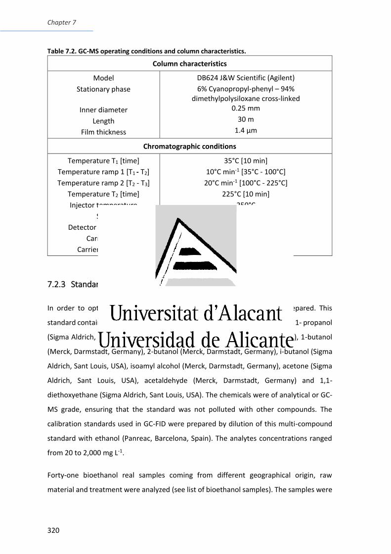
Chapter 7
320
Table 7.2. GC-MS operating conditions and column characteristics.
Column characteristics
Model
Stationary phase
Inner diameter
Length
Film thickness
DB624 J&W Scientific (Agilent)
6% Cyanopropyl-phenyl – 94% dimethylpolysiloxane cross-linked
0.25 mm
30 m
1.4 µm
Chromatographic conditions
Temperature T1 [time]
Temperature ramp 1 [T1 - T2]
Temperature ramp 2 [T2 - T3]
Temperature T2 [time]
Injector temperature
Split
Detector temperature
Carrier gas
Carrier flow rate
35°C [10 min]
10°C min-1 [35°C - 100°C]
20°C min-1 [100°C - 225°C]
225°C [10 min]
250°C
1:10
250°C
He
1.3 mL min-1
7.2.3 Standards and samples.
In order to optimize the separation, a multi-compound standard was prepared. This
standard contained 2,000 mg L-1 of methanol (Sigma Aldrich, Sant Louis, USA), 1- propanol
(Sigma Aldrich, Sant Louis, USA), 2-propanol (Sigma Aldrich, Sant Louis, USA), 1-butanol
(Merck, Darmstadt, Germany), 2-butanol (Merck, Darmstadt, Germany), i-butanol (Sigma
Aldrich, Sant Louis, USA), isoamyl alcohol (Merck, Darmstadt, Germany), acetone (Sigma
Aldrich, Sant Louis, USA), acetaldehyde (Merck, Darmstadt, Germany) and 1,1-
diethoxyethane (Sigma Aldrich, Sant Louis, USA). The chemicals were of analytical or GC-
MS grade, ensuring that the standard was not polluted with other compounds. The
calibration standards used in GC-FID were prepared by dilution of this multi-compound
standard with ethanol (Panreac, Barcelona, Spain). The analytes concentrations ranged
from 20 to 2,000 mg L-1.
Forty-one bioethanol real samples coming from different geographical origin, raw
material and treatment were analyzed (see list of bioethanol samples). The samples were
Determination of VOCs in bioethanol by means of GC-FID and GC-MS
321
grouped in five categories: (i) ten fractions of the distillation of the same bioethanol
sample; (ii) two second-generation bioethanol samples; (iii) one sample of biobutanol (the
main component of the matrix being iso-butanol); (iv) two samples stored in several
materials (glass, Nalgene®, PTFE, HDPE); (v) three samples coming from different raw
materials (winemaking residues, cereal, sugar beet) that have been produced by means
of the same process.
7.3 Results
7.3.1 Quantification of major volatile compounds in bioethanol real samples
by means of GC-FID
7.3.1.1 Method optimization
In a first place, an isothermal program at 65°C was tested for the separation of the 10
compounds present in the multi-compound standard. Under these conditions, the peaks
for some compounds overlapped with the ethanol peak at the beginning of the
chromatogram whereas other compounds were detected at retention times above 50
min. To overcome the peak overlapping simultaneously shortening the analysis time, a
gradient program was set with a 40°C initial temperature for 12 min followed by a
temperature ramp at 5°C min-1 up to 100°C and a third step in which the temperature was
kept at 100°C until the last compound reached the detector. Under these conditions, the
analytes were successfully separated and the analysis time was around 45 min. Finally,
the conditions shown in Table 7.1 were selected as the analysis time of a sample was 30
minutes with good resolution and signal-to-noise ratio. The chromatogram obtained
under these conditions is shown in Figure 7.1. In general terms, the retention time
increased with the boiling point, for a given group of compounds. It is important to remark
that the chromatogram obtained showed an unexpected peak that corresponded to
ethenol originated from the auto-tautomerization of acetaldehyde [21].
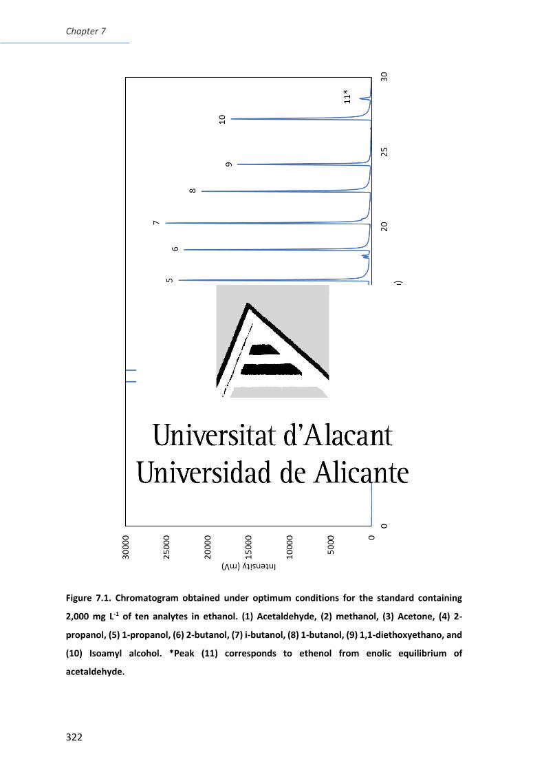
Chapter 7
322
Figure 7.1. Chromatogram obtained under optimum conditions for the standard containing
2,000 mg L-1 of ten analytes in ethanol. (1) Acetaldehyde, (2) methanol, (3) Acetone, (4) 2-
propanol, (5) 1-propanol, (6) 2-butanol, (7) i-butanol, (8) 1-butanol, (9) 1,1-diethoxyethano, and
(10) Isoamyl alcohol. *Peak (11) corresponds to ethenol from enolic equilibrium of
acetaldehyde.
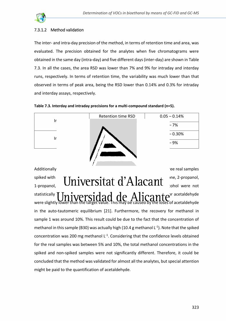
Determination of VOCs in bioethanol by means of GC-FID and GC-MS
323
7.3.1.2 Method validation
The inter- and intra-day precision of the method, in terms of retention time and area, was
evaluated. The precision obtained for the analytes when five chromatograms were
obtained in the same day (intra-day) and five different days (inter-day) are shown in Table
7.3. In all the cases, the area RSD was lower than 7% and 9% for intraday and interday
runs, respectively. In terms of retention time, the variability was much lower than that
observed in terms of peak area, being the RSD lower than 0.14% and 0.3% for intraday
and interday assays, respectively.
Table 7.3. Interday and intraday precisions for a multi-compound standard (n=5).
Intraday Retention time RSD 0.05 – 0.14%
Area RSD 4 – 7%
Interday Retention time RSD 0.09 – 0.30%
Area RSD 7 – 9%
Additionally, the recoveries were obtained by means of the analysis of three real samples
spiked with 200 mg L-1 of the analytes of interest. The recoveries for acetone, 2-propanol,
1-propanol, 2-butanol, 1-butanol, 1,1-diethoxyethane and isoamyl alcohol were not
statistically different from 100% (Figure 7.2). However, the recoveries for acetaldehyde
were slightly lower than the target value. This may be caused by the loses of acetaldehyde
in the auto-tautomeric equilibrium [21]. Furthermore, the recovery for methanol in
sample 1 was around 10%. This result could be due to the fact that the concentration of
methanol in this sample (B30) was actually high (10.4 g methanol L-1). Note that the spiked
concentration was 200 mg methanol L-1. Considering that the confidence levels obtained
for the real samples was between 5% and 10%, the total methanol concentrations in the
spiked and non-spiked samples were not significantly different. Therefore, it could be
concluded that the method was validated for almost all the analytes, but special attention
might be paid to the quantification of acetaldehyde.
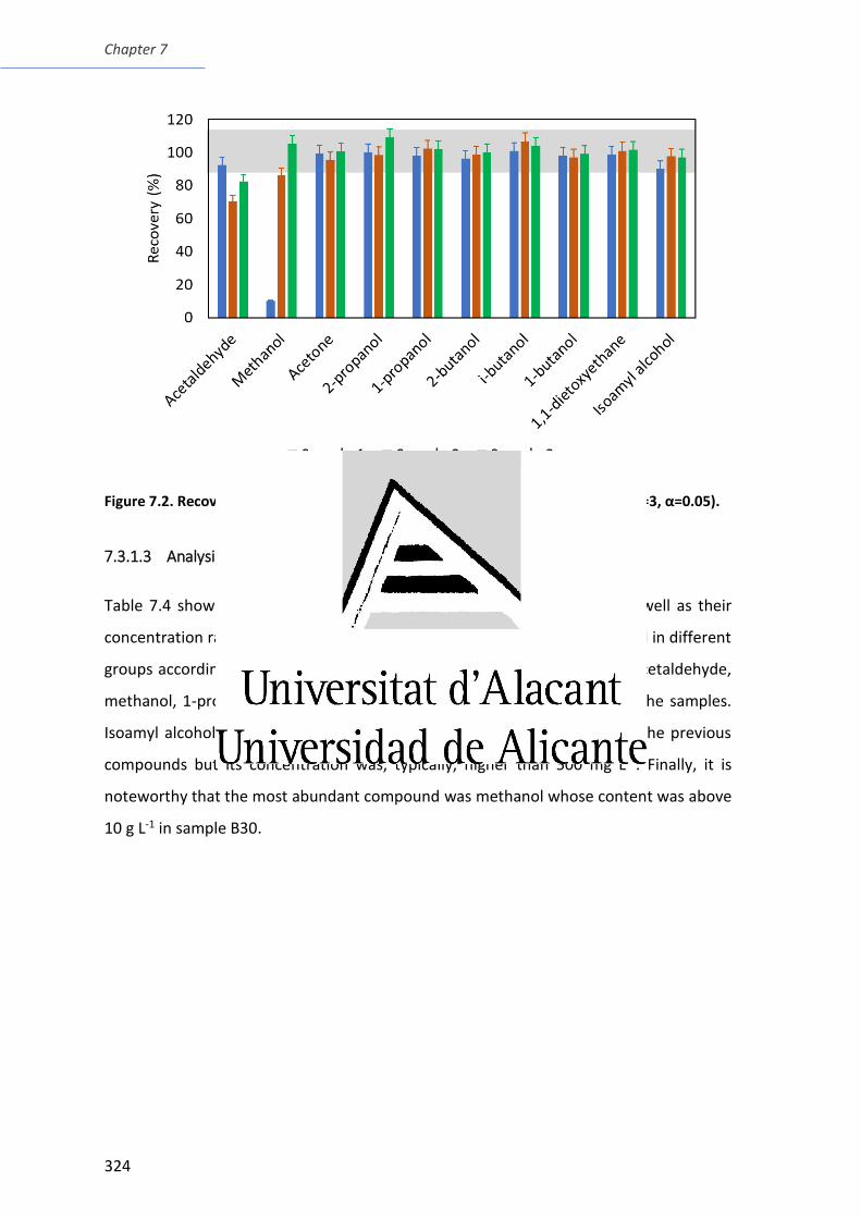
Chapter 7
324
Figure 7.2. Recoveries for three samples spiked with 200 mg L-1 of each analyte (n=3, α=0.05).
7.3.1.3 Analysis of real samples
Table 7.4 shows a summary of the analytes identified in each sample as well as their
concentration range. For the sake of clarity, the samples have been classified in different
groups according to their type. In general terms, it can be observed that acetaldehyde,
methanol, 1-propanol and 1,1-diethoxyethane were present in almost all the samples.
Isoamyl alcohol, in turn, was present in a lower number of samples than the previous
compounds but its concentration was, typically, higher than 500 mg L-1. Finally, it is
noteworthy that the most abundant compound was methanol whose content was above
10 g L-1 in sample B30.
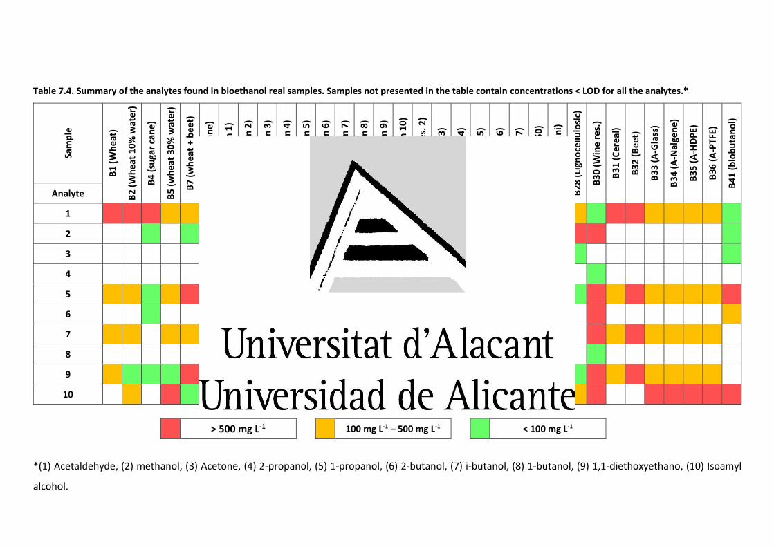
Table 7.4. Summary of the analytes found in bioethanol real samples. Samples not presented in the table contain concentrations < LOD for all the analytes.*
Sam
ple
B1
(W
hea
t)
B2
(W
hea
t 10
% w
ate
r)
B4
(su
gar
can
e)
B5
(w
hea
t 30
% w
ate
r)
B7
(w
hea
t +
bee
t)
B8
(su
gar
can
e)
B9
(Fr
acti
on
1)
B10
(Fr
acti
on
2)
B11
(Fr
acti
on
3)
B12
(Fr
acti
on
4)
B13
(Fr
acti
on
5)
B14
(Fr
acti
on
6)
B15
(Fr
acti
on
7)
B16
(Fr
acti
on
8)
B43
(Fr
acti
on
9)
B42
(Fr
acti
on
10
)
B18
(W
ine
res.
2)
B19
(B
eet
3)
B20
(B
eet
4)
B21
(B
eet
5)
B22
(B
eet
6)
B23
(B
eet
7)
B25
(1
302
50)
B27
(G
uar
ani)
B28
(Li
gno
cellu
losi
c)
B30
(W
ine
res.
)
B31
(C
erea
l)
B32
(B
eet)
B33
(A
-Gla
ss)
B34
(A
-Nal
gen
e)
B35
(A
-HD
PE)
B36
(A
-PTF
E)
B41
(b
iob
uta
no
l)
Analyte
1
2
3
4
5
6
7
8
9
10
> 500 mg L-1 100 mg L-1 – 500 mg L-1 < 100 mg L-1
*(1) Acetaldehyde, (2) methanol, (3) Acetone, (4) 2-propanol, (5) 1-propanol, (6) 2-butanol, (7) i-butanol, (8) 1-butanol, (9) 1,1-diethoxyethano, (10) Isoamyl
alcohol.
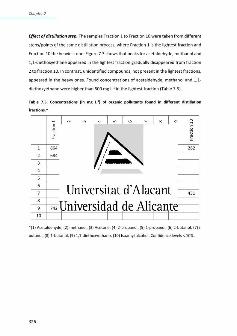
Chapter 7
326
Effect of distillation step. The samples Fraction 1 to Fraction 10 were taken from different
steps/points of the same distillation process, where Fraction 1 is the lightest fraction and
Fraction 10 the heaviest one. Figure 7.3 shows that peaks for acetaldehyde, methanol and
1,1-diethoxyethane appeared in the lightest fraction gradually disappeared from fraction
2 to fraction 10. In contrast, unidentified compounds, not present in the lightest fractions,
appeared in the heavy ones. Found concentrations of acetaldehyde, methanol and 1,1-
diethoxyethane were higher than 500 mg L-1 in the lightest fraction (Table 7.5).
Table 7.5. Concentrations (in mg L-1) of organic pollutants found in different distillation
fractions.*
Frac
tio
n 1
Frac
tio
n 2
Frac
tio
n 3
Frac
tio
n 4
Frac
tio
n 5
Frac
tio
n 6
Frac
tio
n 7
Frac
tio
n 8
Frac
tio
n 9
Frac
tio
n 1
0
1 864 160 282
2 684 315 398 374 186 188
3
4
5 183
6
7 431
8
9 742 325 273
10
*(1) Acetaldehyde, (2) methanol, (3) Acetone, (4) 2-propanol, (5) 1-propanol, (6) 2-butanol, (7) i-
butanol, (8) 1-butanol, (9) 1,1-diethoxyethano, (10) Isoamyl alcohol. Confidence levels < 10%.
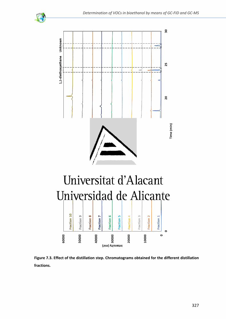
Determination of VOCs in bioethanol by means of GC-FID and GC-MS
327
Figure 7.3. Effect of the distillation step. Chromatograms obtained for the different distillation
fractions.
Chapter 7
328
Effect of storage material. The influence of the material of the container on the
concentration of volatile organic compounds was evaluated. For this purpose, the samples
S8311 and S7875 stored in glass, Nalgene, HDPE and PTFE were analyzed. It was observed
that the storage material did not have any effect on the content of volatile organic
compounds.
Bioethanol samples obtained from different raw materials. Table 7.6 shows the found
concentrations for first generation bioethanol samples obtained using wheat, winemaking
residues, beetroot, cereals and sugar cane as raw materials. It can be observed that
bioethanol produced from winemaking residues (B30) provided the highest contents of
organic pollutants (> 10 g L-1 of methanol, 2.5 g L-1 of 1-propanol and about 2 g L-1 of
butanol isomers). Other samples as B32, B18, B19 or B22 also contained high
concentrations of compounds, such as 1-propanol, 1,1-diethoxyethane and i-butanol.
However, it was not easy to establish a direct link between the raw material and the
pollutants present in the resulting bioethanol. Note that the number of samples produced
from each type of raw material was rather limited.
It should be highlighted that the standard EN15376, which establishes the requirements
for ethanol used as a blending component for automotive fuels [22], reports the
maximum concentrations of methanol allowable at 0.5% and other higher alcohols (C3-
C5) at 2%. Nevertheless, it can be observed that sample B30 contains around 1% of
methanol, which correspond to twice the maximum concentration specified in the
mentioned standard. Some samples also contain significant concentrations of other
alcohols, but they are below the maximum concentration allowable in all the samples
analyzed.
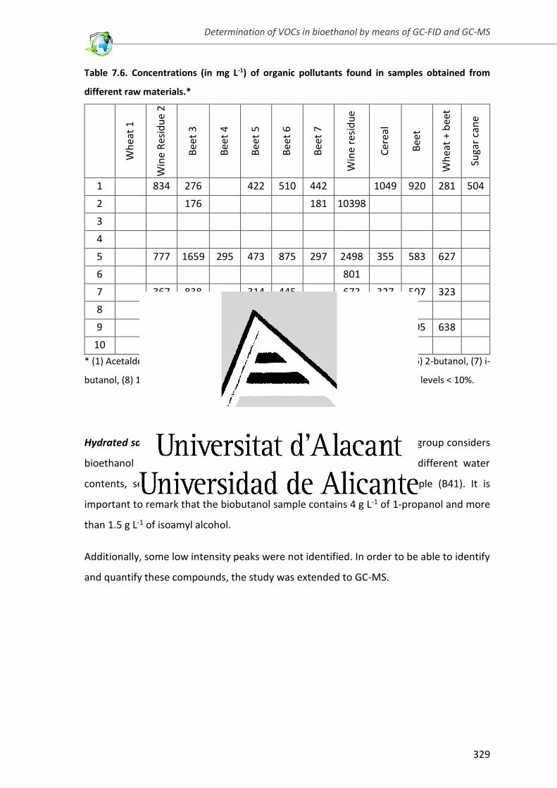
Determination of VOCs in bioethanol by means of GC-FID and GC-MS
329
Table 7.6. Concentrations (in mg L-1) of organic pollutants found in samples obtained from
different raw materials.*
W
hea
t 1
Win
e R
esid
ue
2
Bee
t 3
Bee
t 4
Bee
t 5
Bee
t 6
Bee
t 7
Win
e re
sid
ue
Cer
eal
Bee
t
Wh
eat
+ b
eet
Suga
r ca
ne
1 834 276 422 510 442 1049 920 281 504
2 176 181 10398
3
4
5 777 1659 295 473 875 297 2498 355 583 627
6 801
7 367 838 314 445 673 327 507 323
8
9 737 342 905 638
10 715
* (1) Acetaldehyde, (2) methanol, (3) Acetone, (4) 2-propanol, (5) 1-propanol, (6) 2-butanol, (7) i-
butanol, (8) 1-butanol, (9) 1,1-diethoxyethano, (10) Isoamyl alcohol. Confidence levels < 10%.
Hydrated samples, second generation bioethanol and biobutanol. This group considers
bioethanol obtained by means of different processes, samples with different water
contents, second generation bioethanol (B28) and a biobutanol sample (B41). It is
important to remark that the biobutanol sample contains 4 g L-1 of 1-propanol and more
than 1.5 g L-1 of isoamyl alcohol.
Additionally, some low intensity peaks were not identified. In order to be able to identify
and quantify these compounds, the study was extended to GC-MS.
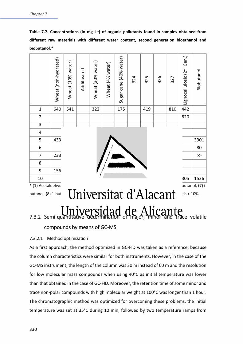
Chapter 7
330
Table 7.7. Concentrations (in mg L-1) of organic pollutants found in samples obtained from
different raw materials with different water content, second generation bioethanol and
biobutanol.*
Wh
eat
(no
n-h
ydra
ted
)
Wh
eat
(10%
wat
er)
Ad
dit
ivat
ed
Wh
eat
(30%
wat
er)
Wh
eat
(4%
wat
er)
Suga
r ca
ne
(40%
wat
er)
B2
4
B2
5
B2
6
B2
7
Lign
oce
llulo
sic
(2n
d G
en.)
.
Bio
bu
tan
ol
1 640 541 322 175 419 810 442
2 820
3
4 117
5 433 407 268 366 589 211 3901
6 80
7 233 376 342 309 >>
8
9 156 365
10 361 712 523 305 1536
* (1) Acetaldehyde, (2) methanol, (3) Acetone, (4) 2-propanol, (5) 1-propanol, (6) 2-butanol, (7) i-
butanol, (8) 1-butanol, (9) 1,1-diethoxyethano, (10) Isoamyl alcohol. Confidence levels < 10%.
7.3.2 Semi-quantitative determination of major, minor and trace volatile
compounds by means of GC-MS
7.3.2.1 Method optimization
As a first approach, the method optimized in GC-FID was taken as a reference, because
the column characteristics were similar for both instruments. However, in the case of the
GC-MS instrument, the length of the column was 30 m instead of 60 m and the resolution
for low molecular mass compounds when using 40°C as initial temperature was lower
than that obtained in the case of GC-FID. Moreover, the retention time of some minor and
trace non-polar compounds with high molecular weight at 100°C was longer than 1 hour.
The chromatographic method was optimized for overcoming these problems, the initial
temperature was set at 35°C during 10 min, followed by two temperature ramps from
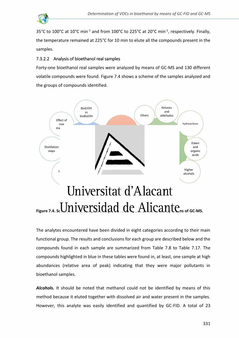
Determination of VOCs in bioethanol by means of GC-FID and GC-MS
331
35°C to 100°C at 10°C min-1 and from 100°C to 225°C at 20°C min-1, respectively. Finally,
the temperature remained at 225°C for 10 min to elute all the compounds present in the
samples.
7.3.2.2 Analysis of bioethanol real samples
Forty-one bioethanol real samples were analyzed by means of GC-MS and 130 different
volatile compounds were found. Figure 7.4 shows a scheme of the samples analyzed and
the groups of compounds identified.
Figure 7.4. Scheme of the samples analyzed and compounds identified by means of GC-MS.
The analytes encountered have been divided in eight categories according to their main
functional group. The results and conclusions for each group are described below and the
compounds found in each sample are summarized from Table 7.8 to Table 7.17. The
compounds highlighted in blue in these tables were found in, at least, one sample at high
abundances (relative area of peak) indicating that they were major pollutants in
bioethanol samples.
Alcohols. It should be noted that methanol could not be identified by means of this
method because it eluted together with dissolved air and water present in the samples.
However, this analyte was easily identified and quantified by GC-FID. A total of 23
Chapter 7
332
additional alcohols such as 1-propanol, 2-butanol, i-butanol, 1- butanol, isoamyl alcohol
and amyl alcohol were present in the samples at relatively high levels (Table 7.8). All these
alcohols were expectedly originated as by-products of the alcoholic fermentation. Some
samples contained heavier alcohols as undecanol or tetradecanol, but their low relative
areas suggested that they were present at trace levels. By means of this analysis, it was
also determined that the main component present in sample B41 (bio-butanol) was i-
butanol instead n-butanol, appearing 1- butanol and 2-butanol as fermentation by-
products.
Aldehydes and ketones. Fifteen analytes containing one of these functional groups were
found in the samples (Table 7.9). The major analyte in this group was acetaldehyde, which
appeared in several samples with a high relative peak area. Most of the analytes of this
group could appear as a consequence of the incomplete fermentation process,
nevertheless, compounds such as acetaldehyde or formaldehyde could be added to water
during the sugars extraction process, to avoid the growth of bacteria, thus remaining in
the final biofuel after the distillation process [23].
Esters. Twenty-four mainly fatty acid ethyl esters (FAEE) were found in the samples (Table
7.10). They were likely the product of the reaction of the organic acids or triacylglicerides,
present in the samples as by-products of the production process, with ethanol at a slightly
acid pH (3.5 < pH < 5.5) (Figure 7.5.a and Figure 7.5.b). The most abundant analytes in this
group were ethyl acetate, ethyl propionate, ethyl butyrate, isoamyl acetate, ethyl valerate
and ethyl caproate. Other esters with higher number of carbon atoms were found but the
areas of the peaks they generated were much lower than those for the previously
mentioned compounds, suggesting that they were present at trace levels. It is noteworthy
that, for sample B41 (bio-butanol), a specific ester profile was found. In this product, some
of the FAEEs found in bioethanol were not present but peaks assigned to fatty acid
isobutyl esters were detected. This fact suggested that fatty acids reacted with iso-
butanol.
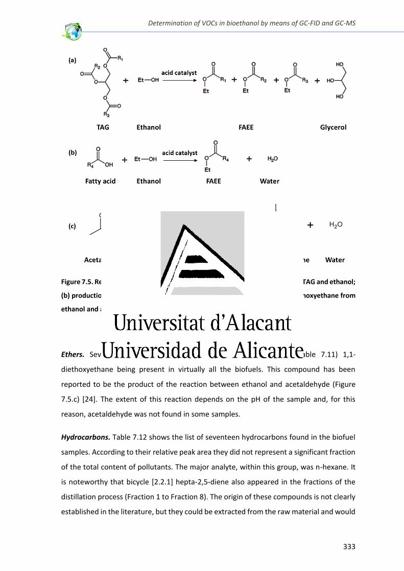
Determination of VOCs in bioethanol by means of GC-FID and GC-MS
333
Figure 7.5. Reactions that take place in bioethanol. (a) generation of FAEE from TAG and ethanol;
(b) production of FAEE from fatty acids and ethanol; (c) generation of 1,1-diethoxyethane from
ethanol and acetaldehyde.
Ethers. Seventeen ethers have been identified in the samples (Table 7.11) 1,1-
diethoxyethane being present in virtually all the biofuels. This compound has been
reported to be the product of the reaction between ethanol and acetaldehyde (Figure
7.5.c) [24]. The extent of this reaction depends on the pH of the sample and, for this
reason, acetaldehyde was not found in some samples.
Hydrocarbons. Table 7.12 shows the list of seventeen hydrocarbons found in the biofuel
samples. According to their relative peak area they did not represent a significant fraction
of the total content of pollutants. The major analyte, within this group, was n-hexane. It
is noteworthy that bicycle [2.2.1] hepta-2,5-diene also appeared in the fractions of the
distillation process (Fraction 1 to Fraction 8). The origin of these compounds is not clearly
established in the literature, but they could be extracted from the raw material and would
Chapter 7
334
remain in the sample after distillation. Another hypothesis is that, some of them, could
be a by-product of the fermentation process or even formed during the fuel storage.
Aromatic hydrocarbons. Twelve aromatic hydrocarbons were detected at moderate
contents (relative areas) in the bioethanol samples (Table 7.13). Toluene and the three
isomers of xylene (m-xylene and p-xylene appeared at the same retention time, whereas
o-xylene eluted at longer times) prevailed over the remaining analytes of this group.
Aromatic hydrocarbons could be probably extracted from the raw material in the first
steps of the bioethanol production process.
Nitrogen compounds. Ten nitrogen compounds were identified in the samples (Table
7.14) but none of them was present under relevant concentrations (relative areas were
very low). The possible origin of the nitrogen compounds was the raw material.
Organic acids. Only two organic acids remained in the samples (Table 7.15), probably
because they were converted into FAEEs at the pH of the samples. These two acids were
acetic acid in a great number of samples and isobutyric acid in the case of sample B41
(bio-butanol) where isobutanol was the main component of the matrix. Organic acids
could appear as a result of the ethanol or isobutanol oxidation during the fermentation
step.
Furane derivates. Sample B28 (lignocellulosic bioethanol) contained eight different
furane derivates (Table 7.16). It should be noted that this sample is a second-generation
bioethanol and the presence of furane and related compounds has been reported to be a
consequence of non-complete fermentations of lignocellulosic ethanol [25].
Additional organic compounds. Six additional compounds were found in the samples that
fell out of the previous groups (Table 7.17). Limonene appeared in a remarkable number
of samples (i.e., fourteen). This compound could be easily extracted from the raw
materials used in the bioethanol production.
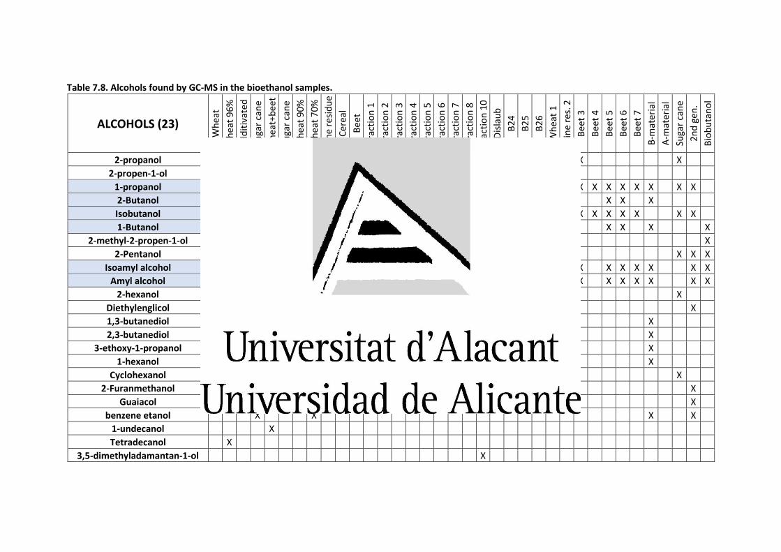
Table 7.8. Alcohols found by GC-MS in the bioethanol samples.
ALCOHOLS
Wh
eat
Wh
eat
96%
Ad
dit
ivat
ed
Suga
r ca
ne
Wh
eat+
bee
t
Suga
r ca
ne
Wh
eat
90%
Wh
eat
70%
Win
e re
sid
ue
Cer
eal
Bee
t
Frac
tio
n 1
Frac
tio
n 2
Frac
tio
n 3
Frac
tio
n 4
Frac
tio
n 5
Frac
tio
n 6
Frac
tio
n 7
Frac
tio
n 8
Frac
tio
n 1
0
Dis
lau
b
B2
4
B2
5
B2
6
Wh
eat
1
Win
e re
s. 2
Bee
t 3
Bee
t 4
Bee
t 5
Bee
t 6
Bee
t 7
B-m
ater
ial
A-m
ater
ial
Suga
r ca
ne
2n
d g
en.
Bio
bu
tan
ol
2-propanol X X X X X X X
2-propen-1-ol X
1-propanol X X X X X X X X X X X X X X X X X X X X X
2-Butanol X X X X X X X X
Isobutanol X X X X X X X X X X X X X X X X X
1-Butanol X X X X X X X X X X X
2-methyl-2-propen-1-ol X
2-Pentanol X X X X
Isoamyl alcohol X X X X X X X X X X X X X X X X X X X
Amyl alcohol X X X X X X X X X X X X X X X X X X X
2-hexanol X
Diethylenglicol X
1,3-butanediol X
2,3-butanediol X X
3-ethoxy-1-propanol X
1-hexanol X X X X
Cyclohexanol X
2-Furanmethanol X X
Guaiacol X
benzene etanol X X X X
1-undecanol X
Tetradecanol X
3,5-dimethyladamantan-1-ol X
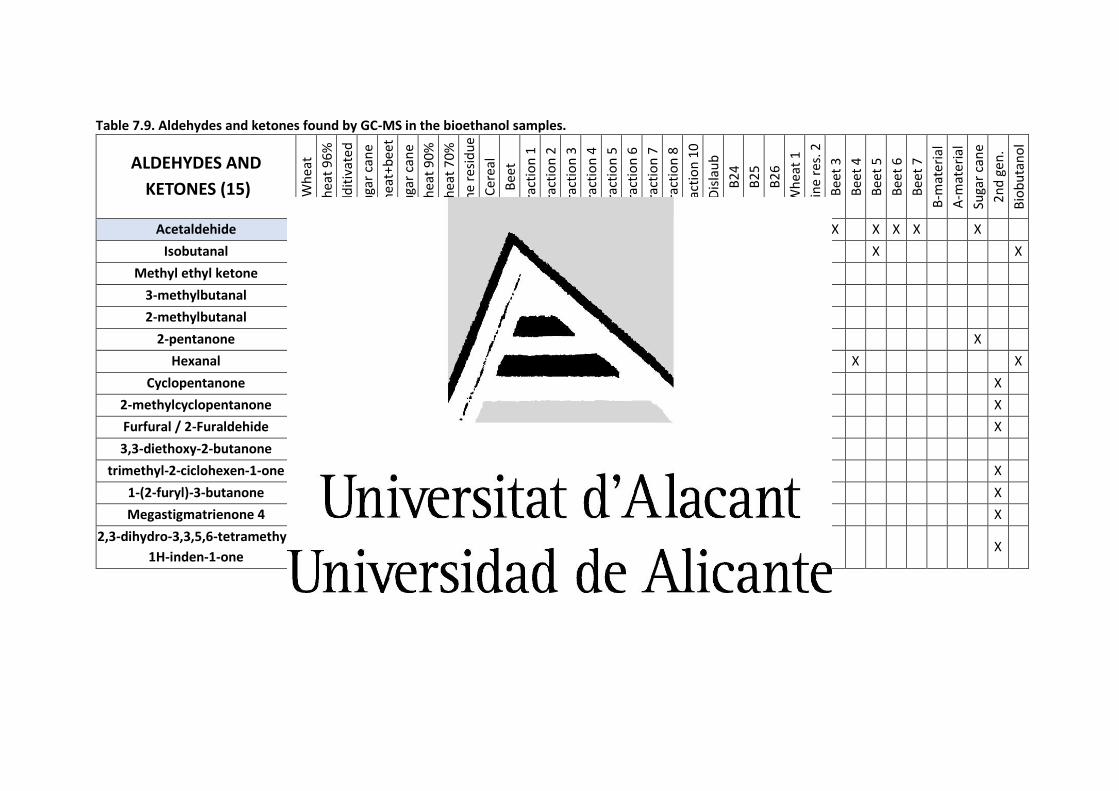
Table 7.9. Aldehydes and ketones found by GC-MS in the bioethanol samples.
ALDEHYDES AND
KETONES Wh
eat
Wh
eat
96%
Ad
dit
ivat
ed
Suga
r ca
ne
Wh
eat+
bee
t
Suga
r ca
ne
Wh
eat
90%
Wh
eat
70%
Win
e re
sid
ue
Cer
eal
Bee
t
Frac
tio
n 1
Frac
tio
n 2
Frac
tio
n 3
Frac
tio
n 4
Frac
tio
n 5
Frac
tio
n 6
Frac
tio
n 7
Frac
tio
n 8
Frac
tio
n 1
0
Dis
lau
b
B2
4
B2
5
B2
6
Wh
eat
1
Win
e re
s. 2
Bee
t 3
Bee
t 4
Bee
t 5
Bee
t 6
Bee
t 7
B-m
ater
ial
A-m
ater
ial
Suga
r ca
ne
2n
d g
en.
Bio
bu
tan
ol
Acetaldehide X X X X X X X X X X X X
Isobutanal X X X
Methyl ethyl ketone X X
3-methylbutanal X
2-methylbutanal X
2-pentanone X
Hexanal X X
Cyclopentanone X
2-methylcyclopentanone X
Furfural / 2-Furaldehide X X
3,3-diethoxy-2-butanone X
trimethyl-2-ciclohexen-1-one X
1-(2-furyl)-3-butanone X
Megastigmatrienone 4 X
2,3-dihydro-3,3,5,6-tetramethyl-
1H-inden-1-one X
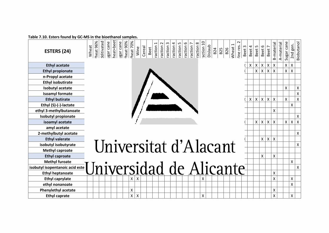
Table 7.10. Esters found by GC-MS in the bioethanol samples.
ESTERS
Wh
eat
Wh
eat
96%
Ad
dit
ivat
ed
Suga
r ca
ne
Wh
eat+
bee
t
Suga
r ca
ne
Wh
eat
90%
Wh
eat
70%
Win
e re
sid
ue
Cer
eal
Bee
t
Frac
tio
n 1
Frac
tio
n 2
Frac
tio
n 3
Frac
tio
n 4
Frac
tio
n 5
Frac
tio
n 6
Frac
tio
n 7
Frac
tio
n 8
Frac
tio
n 1
0
Dis
lau
b
B2
4
B2
5
B2
6
Wh
eat
1
Win
e re
s. 2
Bee
t 3
Bee
t 4
Bee
t 5
Bee
t 6
Bee
t 7
B-m
ater
ial
A-m
ater
ial
Suga
r ca
ne
2n
d g
en.
Bio
bu
tan
ol
Ethyl acetate X X X X X X X X X X X X X X X X X X X X X X X X
Ethyl propionate X X X X X X X X X X X X X X X X X X X X
n-Propyl acetate X
Ethyl isobutirate X
Isobutyl acetate X X
Isoamyl formate X
Ethyl butirate X X X X X X X X X X X X X X X X X X X X X X X X X X
Ethyl (S)-(-)-lactate X X X X
ethyl 3-methylbutanoate X X
Isobutyl propionate X
isoamyl acetate X X X X X X X X X X X X X X X X X X
amyl acetate X
2-methylbutyl acetate X X
Ethyl valerate X X X X X X X X X X
isobutyl isobutyrate X
Methyl caproate X
Ethyl caproate X X X X X X X X X X X X
Methyl furoate X
isobutyl isopentanoic acid ester X
Ethyl heptanoate X X
Ethyl caprylate X X X X X
ethyl nonanoate X
Phenylethyl acetate X X
Ethyl caprate X X X X X
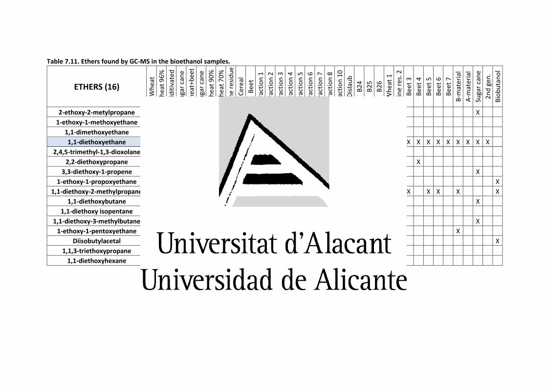
Table 7.11. Ethers found by GC-MS in the bioethanol samples.
ETHERS
Wh
eat
Wh
eat
96%
Ad
dit
ivat
ed
Suga
r ca
ne
Wh
eat+
bee
t
Suga
r ca
ne
Wh
eat
90%
Wh
eat
70%
Win
e re
sid
ue
Cer
eal
Bee
t
Frac
tio
n 1
Frac
tio
n 2
Frac
tio
n 3
Frac
tio
n 4
Frac
tio
n 5
Frac
tio
n 6
Frac
tio
n 7
Frac
tio
n 8
Frac
tio
n 1
0
Dis
lau
b
B2
4
B2
5
B2
6
Wh
eat
1
Win
e re
s. 2
Bee
t 3
Bee
t 4
Bee
t 5
Bee
t 6
Bee
t 7
B-m
ater
ial
A-m
ater
ial
Suga
r ca
ne
2n
d g
en.
Bio
bu
tan
ol
2-ethoxy-2-metylpropane X
1-ethoxy-1-methoxyethane X
1,1-dimethoxyethane X
1,1-diethoxyethane X X X X X X X X X X X X X X X X X X X X X X X X X X X X X
2,4,5-trimethyl-1,3-dioxolane X
2,2-diethoxypropane X X
3,3-diethoxy-1-propene X
1-ethoxy-1-propoxyethane X X
1,1-diethoxy-2-methylpropane X X X X X X X X X X X X X X X X
1,1-diethoxybutane X X X X
1,1-diethoxy isopentane X X
1,1-diethoxy-3-methylbutane X X X
1-ethoxy-1-pentoxyethane X X
Diisobutylacetal X
1,1,3-triethoxypropane X
1,1-diethoxyhexane X
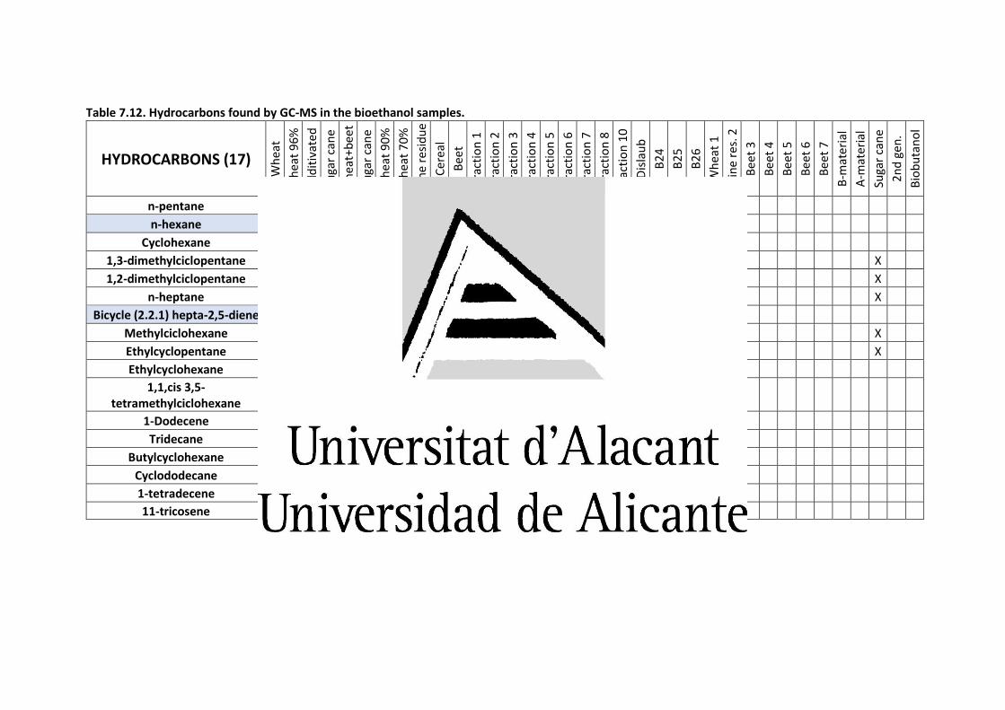
Table 7.12. Hydrocarbons found by GC-MS in the bioethanol samples.
HYDROCARBONS
Wh
eat
Wh
eat
96%
Ad
dit
ivat
ed
Suga
r ca
ne
Wh
eat+
bee
t
Suga
r ca
ne
Wh
eat
90%
Wh
eat
70%
Win
e re
sid
ue
Cer
eal
Bee
t
Frac
tio
n 1
Frac
tio
n 2
Frac
tio
n 3
Frac
tio
n 4
Frac
tio
n 5
Frac
tio
n 6
Frac
tio
n 7
Frac
tio
n 8
Frac
tio
n 1
0
Dis
lau
b
B2
4
B2
5
B2
6
Wh
eat
1
Win
e re
s. 2
Bee
t 3
Bee
t 4
Bee
t 5
Bee
t 6
Bee
t 7
B-m
ater
ial
A-m
ater
ial
Suga
r ca
ne
2n
d g
en.
Bio
bu
tan
ol
n-pentane
n-hexane X X X X X X X X X X X
Cyclohexane X X X X X X
1,3-dimethylciclopentane X
1,2-dimethylciclopentane X
n-heptane X X X X
Bicycle (2.2.1) hepta-2,5-diene X X X X X X X X
Methylciclohexane X
Ethylcyclopentane X
Ethylcyclohexane
1,1,cis 3,5-tetramethylciclohexane
X
1-Dodecene X X
Tridecane X
Butylcyclohexane X
Cyclododecane X
1-tetradecene X X X
11-tricosene X
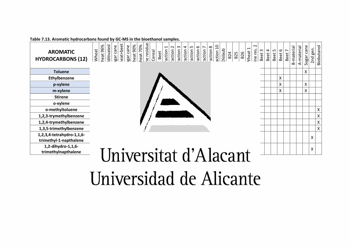
Table 7.13. Aromatic hydrocarbons found by GC-MS in the bioethanol samples.
AROMATIC HYDROCARBONS W
hea
t
Wh
eat
96%
Ad
dit
ivat
ed
Suga
r ca
ne
Wh
eat+
bee
t
Suga
r ca
ne
Wh
eat
90%
Wh
eat
70%
Win
e re
sid
ue
Cer
eal
Bee
t
Frac
tio
n 1
Frac
tio
n 2
Frac
tio
n 3
Frac
tio
n 4
Frac
tio
n 5
Frac
tio
n 6
Frac
tio
n 7
Frac
tio
n 8
Frac
tio
n 1
0
Dis
lau
b
B2
4
B2
5
B2
6
Wh
eat
1
Win
e re
s. 2
Bee
t 3
Bee
t 4
Bee
t 5
Bee
t 6
Bee
t 7
B-m
ater
ial
A-m
ater
ial
Suga
r ca
ne
2n
d g
en.
Bio
bu
tan
ol
Toluene X X X X X X X X X X X X X X X
Ethylbenzene X X X
p-xylene X X X X X X X X X X X X X X X X X X
m-xylene X X X X X X X X X X X X X X X X
Stirene X X X X X X X
o-xylene X X
o-methyltoluene X
1,2,3-trymethylbenzene X X
1,2,4-trymethylbenzene X X
1,3,5-trimethylbenzene X X
1,2,3,4-tetrahydro-1,1,6-trimethyl-1-napthalene
X
1,2-dihydro-1,1,6-trimethylnapthalene
X
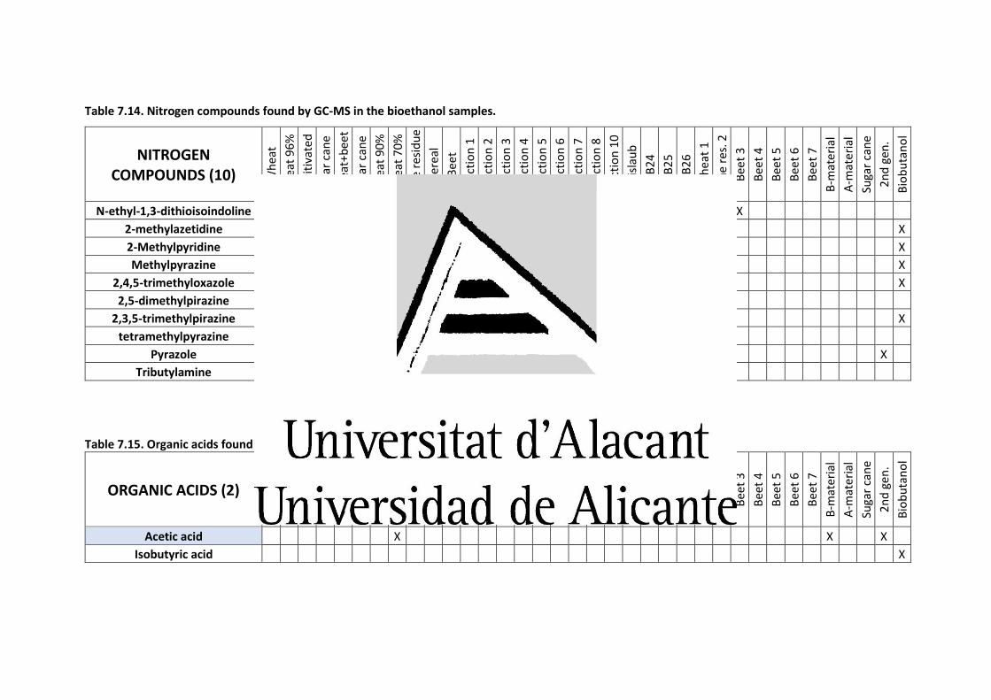
Table 7.14. Nitrogen compounds found by GC-MS in the bioethanol samples.
NITROGEN COMPOUNDS W
hea
t
Wh
eat
96%
Ad
dit
ivat
ed
Suga
r ca
ne
Wh
eat+
bee
t
Suga
r ca
ne
Wh
eat
90%
Wh
eat
70%
Win
e re
sid
ue
Cer
eal
Bee
t
Frac
tio
n 1
Frac
tio
n 2
Frac
tio
n 3
Frac
tio
n 4
Frac
tio
n 5
Frac
tio
n 6
Frac
tio
n 7
Frac
tio
n 8
Frac
tio
n 1
0
Dis
lau
b
B2
4
B2
5
B2
6
Wh
eat
1
Win
e re
s. 2
Bee
t 3
Bee
t 4
Bee
t 5
Bee
t 6
Bee
t 7
B-m
ater
ial
A-m
ater
ial
Suga
r ca
ne
2n
d g
en.
Bio
bu
tan
ol
N-ethyl-1,3-dithioisoindoline X X X X
2-methylazetidine X
2-Methylpyridine X
Methylpyrazine X
2,4,5-trimethyloxazole X
2,5-dimethylpirazine X
2,3,5-trimethylpirazine X
tetramethylpyrazine X
Pyrazole X
Tributylamine X X X X X X X X
Table 7.15. Organic acids found by GC-MS in the bioethanol samples.
ORGANIC ACIDS
Wh
eat
Wh
eat
96%
Ad
dit
ivat
ed
Suga
r ca
ne
Wh
eat+
bee
t
Suga
r ca
ne
Wh
eat
90%
Wh
eat
70%
Win
e re
sid
ue
Cer
eal
Bee
t
Frac
tio
n 1
Frac
tio
n 2
Frac
tio
n 3
Frac
tio
n 4
Frac
tio
n 5
Frac
tio
n 6
Frac
tio
n 7
Frac
tio
n 8
Frac
tio
n 1
0
Dis
lau
b
B2
4
B2
5
B2
6
Wh
eat
1
Win
e re
s. 2
Bee
t 3
Bee
t 4
Bee
t 5
Bee
t 6
Bee
t 7
B-m
ater
ial
A-m
ater
ial
Suga
r ca
ne
2n
d g
en.
Bio
bu
tan
ol
Acetic acid X X X
Isobutyric acid X
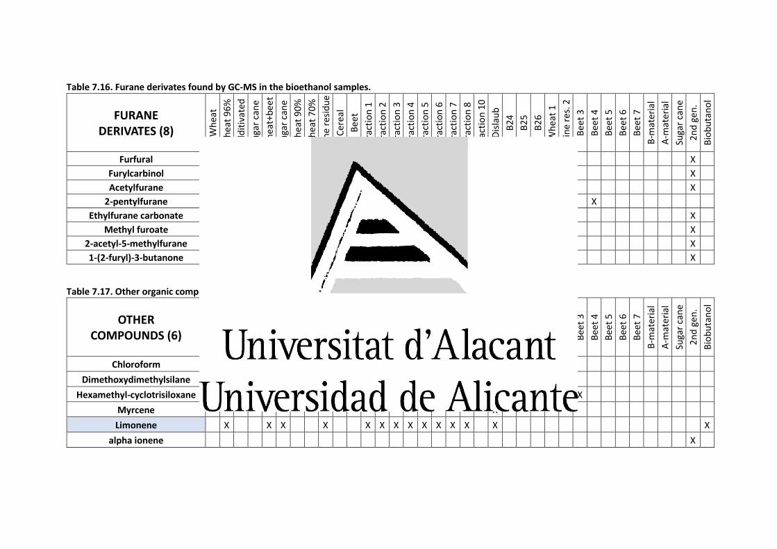
Table 7.16. Furane derivates found by GC-MS in the bioethanol samples.
FURANE DERIVATES W
hea
t
Wh
eat
96%
Ad
dit
ivat
ed
Suga
r ca
ne
Wh
eat+
bee
t
Suga
r ca
ne
Wh
eat
90%
Wh
eat
70%
Win
e re
sid
ue
Cer
eal
Bee
t
Frac
tio
n 1
Frac
tio
n 2
Frac
tio
n 3
Frac
tio
n 4
Frac
tio
n 5
Frac
tio
n 6
Frac
tio
n 7
Frac
tio
n 8
Frac
tio
n 1
0
Dis
lau
b
B2
4
B2
5
B2
6
Wh
eat
1
Win
e re
s. 2
Bee
t 3
Bee
t 4
Bee
t 5
Bee
t 6
Bee
t 7
B-m
ater
ial
A-m
ater
ial
Suga
r ca
ne
2n
d g
en.
Bio
bu
tan
ol
Furfural X X
Furylcarbinol X X
Acetylfurane X
2-pentylfurane X
Ethylfurane carbonate X
Methyl furoate X
2-acetyl-5-methylfurane X
1-(2-furyl)-3-butanone X
Table 7.17. Other organic compounds found by GC-MS in the bioethanol samples.
OTHER COMPOUNDS W
hea
t
Wh
eat
96%
Ad
dit
ivat
ed
Suga
r ca
ne
Wh
eat+
bee
t
Suga
r ca
ne
Wh
eat
90%
Wh
eat
70%
Win
e re
sid
ue
Cer
eal
Bee
t
Frac
tio
n 1
Frac
tio
n 2
Frac
tio
n 3
Frac
tio
n 4
Frac
tio
n 5
Frac
tio
n 6
Frac
tio
n 7
Frac
tio
n 8
Frac
tio
n 1
0
Dis
lau
b
B2
4
B2
5
B2
6
Wh
eat
1
Win
e re
s. 2
Bee
t 3
Bee
t 4
Bee
t 5
Bee
t 6
Bee
t 7
B-m
ater
ial
A-m
ater
ial
Suga
r ca
ne
2n
d g
en.
Bio
bu
tan
ol
Chloroform X
Dimethoxydimethylsilane X
Hexamethyl-cyclotrisiloxane X X X X X X X
Myrcene X
Limonene X X X X X X X X X X X X X X
alpha ionene X
Determination of VOCs in bioethanol by means of GC-FID and GC-MS
343
Additionally, Figure 7.6 shows the number of samples in which each analyte was
identified. The number of pollutants that was found in the samples was very high (130
organic compounds in 41 samples). However, none of them was present in every sample.
These two facts, revealed that bioethanol production is complex and slight modifications
in this process as well as in the raw material used as source of sugars, may cause an
alteration of the organic pollutants contained in the final bioethanol. In addition, the
storage and transport conditions (i.e., temperature, pH, humidity, hydration grade of
bioethanol, etc.) could strongly affect the organic fraction of the bioethanol samples, since
some of the pollutants were products resulting from post-production chemical reactions.
It should also be noted that alcohols and esters, generated by reaction of organic acids
and alcohols, appeared as the predominant groups of pollutants in bioethanol samples in
terms of both, total number of compounds and concentration. Surprisingly, the most
frequent pollutant was an ether (1,1-diethoxyethane) that was present in 35 products
(85% of the samples).
Other groups of compounds, such as hydrocarbons, aromatic hydrocarbons and
heterocycles, have been found at minor or trace levels in a considerable number of
samples. However, it should be taken into account that these compounds (VOCs) can
severely affect the environment quality and the human health [26,27] even at very low
concentrations. Some aromatic hydrocarbons identified in the samples, such as benzene,
toluene, ethylbenzene and xylene (BTEX), have been widely recognized as human
carcinogens whereas others also possess high toxicity, especially to central nervous
system in humans [26]. Moreover, acetaldehyde was also present in a significant number
of bioethanol samples. This fact could explain the data reported by Niven [10] related with
an increase of acetaldehyde emissions when 10% ethanol was added to gasoline (E10).
Nevertheless, in the same study, it was reported that the addition of ethanol to gasoline
lowered, compared with pure gasoline, the emission of other VOCs, such as xylene or
toluene [10].
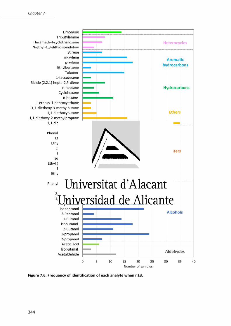
Chapter 7
344
Figure 7.6. Frequency of identification of each analyte when n≥3.
Determination of VOCs in bioethanol by means of GC-FID and GC-MS
345
Regarding the number of pollutants found in the analyzed biofuels, sample B30 (i.e., a
bioethanol originated from winemaking wastes), yielded the highest number of peaks. A
total of 37 compounds (together with methanol that could not be identified in the present
work by GC-MS) were identified in this sample (Figure 7.7). Additional samples, as
biobutanol (B41) or the second-generation bioethanol (B28) also contained a high number
of organic compounds in their matrices. Each one of these samples showed more than 30
peaks in GC-MS. Finally, around 25 organic pollutants were detected in samples such as
B1, B5, B27, and the set from B33 to B36, whereas the rest of the samples contained less
than 25 organic compounds (Figure 7.7).
In the present study, some samples were selected to evaluate the effect of different
variables on the number of organic compounds in the samples and their concentrations.
Distillation fractions (Fraction 1 to Fraction 8) were considered (Figure 7.8). As it was
established in GC-FID for major pollutants, it can be clearly observed that some volatile
organic compounds were more concentrated in the lightest fraction and their
concentration decreased in heavier fractions. It can be clearly observed in the cases of:
acetaldehyde (Figure 7.8.b), ethyl acetate (Figure 7.8.c), bicycle [2.2.1] hepta-2,5-diene
and 1,1-diethoxyethane and toluene (Figure 7.8.d). There is a direct relation between the
boiling point and the fractions where these analytes were present. Acetaldehyde, whose
boiling point is 20.2°C, was only detected in the initial fractions (1 and 2). Ethyl acetate,
with a boiling point of 77°C appeared in fractions from 1 to 3. However, bicycle [2.2.1]
hepta-2,5-diene (b.p.:89°C), 1,1-diethoxyethane (b.p.:102°C) and toluene (b.p.:111°C)
were present in all the fractions, except the heaviest one (fraction 10) under different
concentrations.
Several samples provided by the company UNGDA coming from several raw materials
have also been studied in detail (Figure 7.9). These samples are B30, obtained from wine
by-products, B31, obtained using cereals as raw material and B32, generated using sugars
extracted from beetroot. The sample B30 contained 37 different organic compounds
whereas the samples coming from cereals and beetroot were cleaner with 14 and 18
volatile organic compounds, respectively.
Chapter 7
346
Regarding the effect of the storage material, as it was observed for major pollutants, the
profile of minor and trace organic compounds was not affected by the storage material.
The comparison between first-generation and second-generation bioethanol was also
very interesting. The second-generation sample (B28) contained a large number of
organic compounds within its matrix (33 compounds), typically higher than the average
number of organic pollutants in the first-generation samples. Unfortunately, only one
representative sample originated from lignocellulosic material (second-generation) was
available in this study. However, other samples (e.g., B30, obtained from winemaking sub-
products, with 37 compounds present in its matrix) were more polluted than B28. This
topic could be source of further discussion, since some authors consider bioethanol
obtained from sub-products of other process as second-generation despite they are not
obtained from lignocellulosic material. Therefore, if sample B30 is considered as second-
generation bioethanol, it could be concluded that second-generation samples presented
higher number of organic pollutants than first-generation bioethanol.
The estimated total concentration of VOCs in sample B30, the most polluted one, was
about 25 g of VOCs L-1. This content corresponded to a 2.5% of the sample, revealing the
significant contribution of this kind of organic compounds to the composition of some
bioethanol samples. It should also be noted that the concentration of VOCs found in
sample B30 is higher than that established as the maximum allowable in the standard
EN15376 [22].
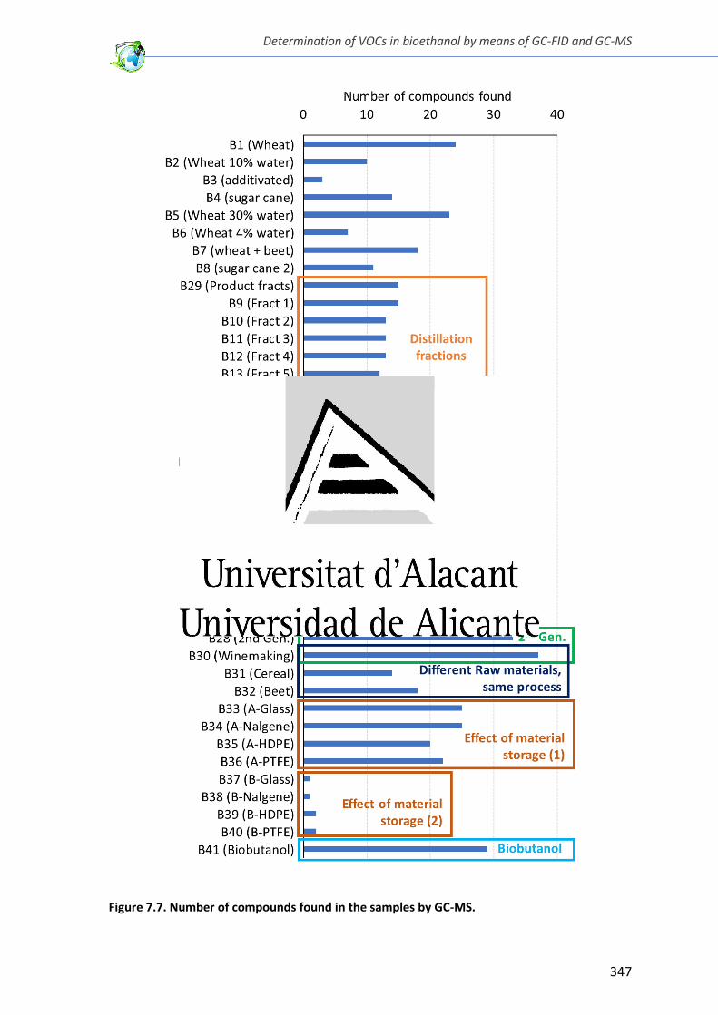
Determination of VOCs in bioethanol by means of GC-FID and GC-MS
347
Figure 7.7. Number of compounds found in the samples by GC-MS.
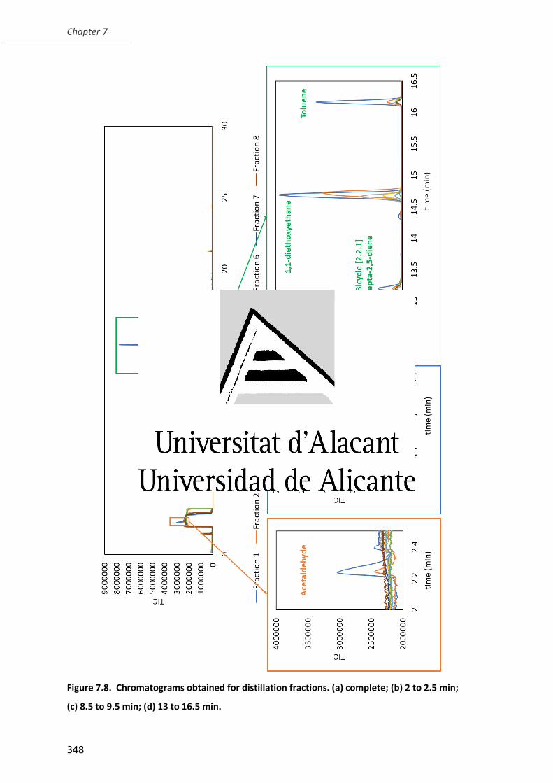
Chapter 7
348
Figure 7.8. Chromatograms obtained for distillation fractions. (a) complete; (b) 2 to 2.5 min;
(c) 8.5 to 9.5 min; (d) 13 to 16.5 min.
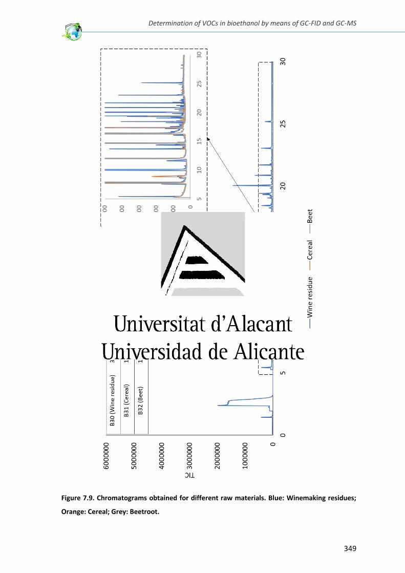
Determination of VOCs in bioethanol by means of GC-FID and GC-MS
349
Figure 7.9. Chromatograms obtained for different raw materials. Blue: Winemaking residues;
Orange: Cereal; Grey: Beetroot.
Chapter 7
350
7.4 Conclusions.
More than 130 different VOCs were identified in bioethanol samples. Some of these
pollutants can be directly extracted from the raw material, such as limonene, organic acids
and aromatic hydrocarbons. Nevertheless, other VOCs, such as alcohols or acetaldehyde,
appear as by-products of the fermentation process. Finally, other group of organic
compounds can be generated in the samples after their production by means of reactions
favored by slightly acid conditions. Among these compounds esters (especially FAEEs) and
1,1-diethoxyethane, present in almost all the samples, are found. These results indicate
that bioethanol samples have a complex matrix, with variable water content and VOCs in
concentrations in the order of tens of g L-1 (the total amount of VOCs in bioethanol
samples was up to 2.5%). These results highlight the difficulty in removing matrix effects
in ICP techniques when analyzing bioethanol samples. Likewise, systems such as the
hTISIS, overcoming these interferences are needed to achieve accurate results.
It has been demonstrated that the material in which the sample is stored does not have
any effect in the organic compounds profile of the sample. Additionally, it has been
reported that those organic compounds with low boiling point (lower or similar that
ethanol b.p.) appear in the bioethanol samples because the distillation is not effective for
their removal. Moreover, second generation sample and bioethanol coming from
winemaking residues presented the highest number of organic compounds in their
matrices. When simple sugars sources as cereals, wheat or beetroot are selected to
produce the bioethanol, less organic pollutants are identified. These results can be
associated with a simple fermentation and it is, consequently, reflected in the lower
number of by-products resulting from this process. Finally, i-butanol was identified as
major component of the matrix of a biobutanol sample. The number of organic
compounds was also higher than the average in the rest of the samples. This fact could
also be associated with the production process, which is more complex than in the case
of first-generation bioethanol.
Alcohols and esters were the most important contributors to the total VOCs in the
bioethanol samples analyzed. However, it is also necessary to carefully monitor other
minor and trace VOCs that have been identified in bioethanol samples, such as benzene,
Determination of VOCs in bioethanol by means of GC-FID and GC-MS
351
toluene, ethylbenzene or xylene (BTEX), since they can cause drastic damages to the
human health when they are emitted to the atmosphere, even in very low concentrations.
All these observations revealed the importance of carrying out the production of
bioethanol under controlled conditions, since slight changes in any of the steps may
modify the profile of organic compounds present in the final product. Additionally, the
conditions of transportation and storage of this biofuel should also be controlled, because
some of the organic products are produced as post-production reactions and changes of
pH, humidity or temperature could modify the concentration of VOCs, and therefore, the
quality of the bioethanol can be altered. On this subject, the metal determination
(chapters 3 and 4) is extremely important as some of them play an active role in terms of
side reactions production. Thus, for instance copper may catalyze ethanol oxidation
reactions thus promoting the appearance of additional organic pollutants.
Chapter 7
352
7.5 References
[1] A. Demirbas, Competitive liquid biofuels from biomass, Appl. Energy. 88 (2011) 17–
28.
[2] M. Köpke, P. Dürre, Biochemical production of bioethanol., in: Handb. Biofuels
Prod. Process. Technol., Woodhead Publishing Limited, 2011: pp. 221–257.
[3] G.M. Walker, Bioethanol: Science and technology of fuel alcohol, Ventus Publishing
ApS, 2010.
[4] E. Wheals, L.C. Basso, D.M. Alves, H. V Amorim, Fuel ethanol after 25 years., Trends
Biotechnol. 17 (1999) 482–487
[5] R. Sánchez, C. Sánchez, C.P. Lienemann, J.L. Todolí, Metal and metalloid
determination in biodiesel and bioethanol, J. Anal. At. Spectrom. 30 (2015) 64–101.
[6] F. Monot, A. Margeot, B. Hahn-Hägerdal, J. Lindstedt, R. Slade, The NILE Project —
Advances in the Conversion of Lignocellulosic Materials into Ethanol, Oil Gas Sci.
Technol. – Re . d’IFP E e gies Nou . 6 693–705.
[7] P. Le os, F.C. Mes uita, Futu e of Glo al Bioetha ol : A App aisal of Results , Risk
and Uncertainties, in: Glob. Bioethanol, Elsevier Inc., 2016: pp. 221–237.
[8] M. Balat, H. Balat, Recent trends in global production and utilization of bio-ethanol
fuel, Appl. Energy. 86 (2009) 2273–2282.
[9] P.S. Nigam, A. Singh, Production of liquid biofuels from renewable resources, Prog.
Energy Combust. Sci. 37 (2011) 52–68.
[10] R.K. Niven, Ethanol in gasoline: Environmental impacts and sustainability review
article, Renew. Sustain. Energy Rev. 9 (2005) 535–555.
[11] J. Fargione, J. Hill, D. Tilman, S. Polasky, P. Hawthorne, Land Clearing and the Biofuel
Carbon Debt, Science. 319 (2008) 1235–1238.
[12] D.P. Ho, H.H. Ngo, W. Guo, A mini review on renewable sources for biofuel,
Determination of VOCs in bioethanol by means of GC-FID and GC-MS
353
Bioresour. Technol. 169 (2014) 742–749.
[13] V. Patil, K.Q. Tran, H.R. Giselrød, Towards sustainable production of biofuels from
microalgae, Int. J. Mol. Sci. 9 (2008) 1188–1195.
[14] H. Habe, T. Shinbo, T. Yamamoto, S. Sato, H. Shimada, K. Sakaki, Chemical Analysis
of Impurities in Diverse Bioethanol Samples, J. Japan Pet. Inst. 56 (2013) 414–422.
[15] C. Sánchez, C.P. Lienemann, J.L. Todolí, Analysis of bioethanol samples through
Inductively Coupled Plasma Mass Spectrometry with a total sample consumption
system, Spectrochim. Acta Part B At. Spectrosc. 124 (2016) 99–108.
[16] C. Sánchez, C.P. Lienemann, J.L. Todolí, Metal and metalloid determination in
bioethanol through inductively coupled plasma-optical emission spectroscopy,
Spectrochim. Acta Part B At. Spectrosc. 115 (2016) 16–22.
[17] D. Chiche, C. Diverchy, A.C. Lucquin, F. Porcheron, F. Defoort, Synthesis Gas
Purification, Oil Gas Sci. Technol. – Re . d’IFP E e gies Nou . 68 (2013) 707–723.
[18] L.G. Anderson, Ethanol fuel use in Brazil: air quality impacts, Energy Environ. Sci. 2
(2009) 1015–1037.
[19] D. Styarini, Y. Aristiawan, F. Aulia, H. Abimanyu, Y. Sudiyani, Determination of
organic impurities in lignocellulosic bioethanol product by GC-FID, Energy Procedia.
32 (2013) 153–159.
[20] C. Sánchez, C.P. Lienemann, J.L. Todolí, Metal and metalloid determination in
bioethanol through inductively coupled plasma-optical emission spectroscopy,
Spectrochim. Acta - Part B At. Spectrosc. 115 (2016).
[21] B. Sulzberger, D. Postma, R. Jakobsen, S.G. Benner, S. Fendorf, O. Larsen, K.M.
Rosso, M. Dupuis, a Hoel, G. a Niklasson, C.G. Granqvist, N.F. Mott, M.J. Apted, M.
Chergui, D.E. Janney, R.C. Gerkin, P.R. Buseck, D.B. Liston, J. a Lovejoy, H. Deng, J.Z.
Zhang, M. Hilgendorff, a P. Yartsev, F. Farges, F. Martin, G. Fagheraz, F. Gazzarrini,
G. Lanzavecchia, G. Sironi, P. Belleville, J.P. Jolivet, J. Livage, M. Myers, K. a Bosnik,
L.E. Brus, B. Ravel, J.J. Rehr, S.D. Conradson, J.F. Meunier, M. Instrumentation, G.
Chapter 7
354
Jennings, Photo-Tautomerization of Acetaldehyde, 337 (2012) 1203–1206.
[22] European Committee for Standardization, EN 15376:2014: Automotive Fuels -
Ethanol as a blending component for automotive fuels - Requirements and test
methods, 2014.
[23] C. Sánchez, J.P. Vidal, C.P. Lienemann, J.L. Todolí, Evolution of the metal and
metalloid content along the bioethanol production process, Fuel Process. Technol.
173 (2018) 1–10.
[24] M.F. Gomez, L.A. Arrúa, M.C. Abello, Synthesis of 1,1-diethoxyethane from
bioethanol. Influence of catalyst acidity, React. Kinet. Catal. Lett. 73 (2001) 143–
149.
[25] G.J. Shin, S.Y. Jeong, J.W. Lee, Evaluation of antioxidant activity of the residues
generated from ethanol concentration of lignocellulosic biomass using
pervaporation, J. Ind. Eng. Chem. 52 (2017) 51–58.
[26] X. Han, L.P. Naeher, A review of traffic-related air pollution exposure assessment
studies in the developing world, Environ. Int. 32 (2006) 106–120.
[27] K. Zhang, S. Batterman, Air pollution and health risks due to vehicle traffic, Sci. Total
Environ. 450–451 (2013) 307–316.

GENERAL CONCLUSIONS

General conclusions
357
From the present PhD, several conclusions can be drawn:
▪ The quantification of metals in bioethanol is a complex task due to the appearance
of matrix effects caused by varying the matrix composition of this kind of samples.
Indeed, the content, of water, organic compounds and inorganic species may
change significantly among samples. These matrix effects are mainly related with
the diffe e es of a alyte t a spo t effi ie y εn) induced by modifications in the
physical properties of the samples.
▪ The use of the high temperature Torch Integrated Sample Introduction System
(hTISIS) operated in both injection modes (continuous sample aspiration at 25-30
µL min-1 or air-segmented injection of 5 µL of sample), coupled to ICP techniques
provides a significant enhancement of sensitivity and a reduction in the extent of
memory effects, in comparison with a conventional sample introduction system.
▪ Heating the hTISIS single pass spray chamber above 300°C makes the analyte
transport efficiency to be virtually 100% regardless the ethanol content.
▪ The hTISIS, operated under optimum temperature conditions, removes the ICP-
OES matrix effects for ethanol-water mixtures. Therefore, this device makes it
possible to perform the direct analysis of bioethanol samples through external
calibration using multielemental standards whose matrix contains ethanol and
water in a 1:1 ratio.
▪ The hTISIS does not remove the ICP-MS ethanol matrix effects. This fact is caused
by the different spatial distribution of the ions in the plasma depending on the
sample ethanol concentration. Therefore, a modification of the relative position
between the torch and the interface (sampling zone) is needed. In conclusion, the
accurate ICP-MS analysis of bioethanol involves moving the plasma torch 1 mm
down plasma axis, using the hTISIS at temperatures above 300°C, diluting the
samples with ultrapure water in a 1:1 proportion and using 1:1 water : ethanol
multielemental standards.
▪ Using the hTISIS, sixteen metals have been quantified in concentrations ranging
from 1 ng mL-1 to 2 µg mL-1 in bioethanol samples. Aluminum, cadmium, calcium,
chromium, copper, iron, magnesium, manganese, potassium, sodium, nickel and
zinc were quantified through ICP-OES, whereas, cobalt, copper, indium, iron,
358
magnesium, manganese, nickel, silver, sodium, strontium and zinc were
encountered in ICP-MS in concentrations above the LOQ. There has not been a
direct link between the type of bioethanol and the number of metals contained
and/or their concentrations.
▪ Among the different possible sources of metals, the raw material has been
identified as the main responsible of the presence of metals in the final product
(bioethanol).
▪ Carbonation and liming steps are applied in the bioethanol production process
prior to fermentation. These processes are efficient for the removal of major
divalent and trivalent cations. However, minor metals and monovalent cations
remain after these procedures. The distillation, carried out after fermentation, is,
in turn, responsible for the removal of more than 99.9% of the metals content.
Note that these species are present in bioethanol in concentrations below 2 mg L-
1 whereas the biomass used for its production contains metals at levels higher than
1 g kg-1.
▪ The use of the hTISIS at 125°C coupled to MC-ICP-MS, using an X-type skimmer,
provides precise and accurate lead isotope ratios in bioethanol samples. This
method affords direct isotopic analysis of this kind of samples without any prior
analyte and sample matrix separation step. Moreover, procedures such as matrix-
matching are not required for the correction of the mass bias. In fact, a standard
prepared in 75% of ethanol successfully performs the mass bias correction in the
60% to 100% ethanol concentration range.
▪ The isotopic analysis of lead in bioethanol samples provides useful information
about the type of biomass used for its production and helps to discern whether a
given sample belongs to first or second bioethanol generation.
▪ Besides water and ethanol, bioethanol contains a wide variety of organic
compounds. The type and concentration of organic compounds in bioethanol
depend on the biomass used for its production and the process applied to convert
this biomass into fuel. Around 130 volatile organic compounds have been
identified in bioethanol samples. This fact shows the importance of developing
new methods free of matrix effects, for the determination of metals in bioethanol.
General conclusions
359
▪ In summary, the present research incorporates new methods for the analysis of
bioethanol. In particular, new methodologies for the quantification of metals
(major, minor and traces) as well as for the lead isotopic analysis of this type of
samples have been developed. These methods provide significant improvements
over the existing ones, in terms of limits of detection and matrix effects. Moreover,
this work has provided new data about the composition of bioethanol regarding
the metals and organic compounds present together with their concentrations as
well as the origin of the formers in this type of samples.


CONCLUSIONES GENERALES

Conclusiones generales
363
A continuación, se detallan las principales conclusiones derivadas de la investigación
realizada en la presente Tesis Doctoral:
▪ La determinación de metales en bioetanol es una tarea compleja debido a los
efectos de matriz causados por la naturaleza variable de la matriz de las muestras
englobadas bajo la denominación de bioetanol. Este hecho se debe a que el
contenido en agua y otros componentes, tanto inorgánicos como orgánicos puede
cambiar de una muestra a otra. Dichos efectos de matriz están relacionados,
principalmente, con las diferencias en eficiencia de transporte de analito (εn) que
se originan como consecuencia de las diferentes propiedades físicas que confieren
a las muestras de bioetanol sus distintas matrices.
▪ El empleo del sistema de consumo total de muestra hTISIS (high temperature
Torch Integrated Sample Introduction System), en ambos modos de introducción
de muestras (aspiración continua a 25-30 µL min-1 o inyección segmentada de 5 µL
de muestra), acoplado a técnicas basadas en ICP proporciona una mejora notable
en sensibilidad y efectos de memoria, en comparación con un sistema de
introducción de muestras convencional.
▪ Cuando la cámara de nebulización de paso simple, que forma parte del sistema
hTISIS, es calentada a temperaturas iguales o superiores a 300°C, la eficiencia de
transporte de analito para cualquier mezcla etanol-agua y, por tanto, muestras de
bioetanol, es la misma y, prácticamente, del 100%.
▪ El uso del sistema de introducción de muestras hTISIS, en condiciones óptimas de
temperatura, acoplado a ICP-OES es capaz de eliminar los efectos de matriz para
cualquier mezcla etanol-agua y, por tanto, muestras de bioetanol. En
consecuencia, este dispositivo posibilita llevar a cabo el análisis de este tipo de
muestras, de forma directa, mediante calibrado externo con patrones que
contienen etanol y agua en una proporción 1:1.
▪ El sistema hTISIS a elevadas temperaturas no elimina los efectos de matriz
causados por el etanol en ICP-MS. El motivo de esta observación radica en que
existe una diferente distribución espacial de los iones en el seno del plasma en
función de la concentración de etanol en la muestra. Por lo tanto, es necesario
modificar la posición relativa de la antorcha con respecto a la interfaz (zona de
364
muestreo) para eliminar los efectos de matriz provocados por el etanol. Bajo estas
condiciones, se puede llevar a cabo el análisis de muestras de bioetanol realizando
una dilución 1:1 de las mismas con agua ultrapura mediante calibrado externo
empleando patrones que contienen agua y etanol en la misma proporción.
▪ Empleando el hTISIS acoplado a ICP-OES e ICP-MS, Se han cuantificado un total de
16 metales en muestras diferentes de bioetanol, en concentraciones que varían
desde el orden de 1 ng mL-1 hasta 2 µg mL-1. En ICP-OES, se han cuantificado
aluminio, cadmio, calcio, cromo, cobre, hierro, magnesio, manganeso, potasio,
sodio, níquel y zinc, mientras que en ICP-MS, se han encontrado cobalto, cobre,
indio, hierro, magnesio, manganeso, níquel, plata, sodio, estroncio y zinc en
concentraciones superiores al LOQ. No se ha encontrado una relación directa
entre el tipo de muestra y el número de metales presentes en las mismas y/o sus
concentraciones.
▪ De entre las diferentes posibilidades, el material de partida ha sido identificado
como el principal factor responsable de la presencia de metales en el producto
final (bioetanol).
▪ Las etapas de eliminación de metales previas a la fermentación empleada en el
proceso de producción de bioetanol, tales como la carbonatación y el encalado,
resultan eficientes para llevar a cabo la eliminación de cationes divalentes y
trivalentes mayoritarios. Sin embargo, no son capaces de extraer metales
minoritarios ni cationes monovalentes. No obstante, la destilación, realizada tras
la fermentación, reduce el contenido en metales en más de un 99.9%,
encontrándose estos en concentraciones inferiores a 2 mg L-1 en bioetanol,
mientras que en la biomasa están presentes en concentraciones superiores a 1 g
Kg-1.
▪ El uso del sistema de introducción de muestras hTISIS a 125°C acoplado a MC-ICP-
MS, empleando un skimmer tipo X, proporciona relaciones isotópicas de plomo
precisas y exactas en muestras de bioetanol. Mediante este método se puede
llevar a cabo el análisis isotópico directo de este tipo de muestras sin separación
previa del analito y la matriz. Además, con objeto de corregir la discriminación en
masa, no es necesario llevar a cabo la igualación exhaustiva de la matriz del patrón
empleado a las de las muestras. De hecho, un patrón preparado en 75% de etanol
Conclusiones generales
365
es capaz de corregir la discriminación en masa en un intervalo de concentraciones
de etanol entre el 60% y el 100%.
▪ El análisis isotópico de plomo en muestras de bioetanol proporciona información
útil sobre el tipo de biomasa empleada para su producción y, por tanto, sobre la
generación a la que pertenece el bioetanol que se está analizando.
▪ La técnica de cromatografía de gases, utilizando un detector de ionización en llama
o un espectrómetro de masas, puede ser empleada para identificar y cuantificar la
mayor parte de compuestos orgánicos volátiles presentes en muestras de
bioetanol.
▪ A pesar de que una matriz de bioetanol tiene como componentes mayoritarios
etanol y agua, se ha demostrado que las muestras de bioetanol presentan una
amplia variedad de compuestos orgánicos. La concentración y tipo de los mismos
depende de la biomasa empleada para su producción y del proceso que haya
sufrido la biomasa para ser convertida en bioetanol. Se han identificado alrededor
de 130 compuestos orgánicos en muestras de bioetanol. Este hecho pone de
manifiesto la importancia que posee el desarrollo de métodos libres de efectos de
matriz para la determinación de metales en bioetanol.
▪ En términos generales, el presente trabajo de investigación aporta nuevos
métodos de análisis de bioetanol. Más concretamente, se han desarrollado
métodos para la cuantificación de metales (mayoritarios, minoritarios y traza) así
como el análisis isotópico de plomo en este tipo de muestras. Estos métodos
proporcionan mejoras notables, frente a los existentes hasta la fecha, en términos
de límites de detección y efectos de matriz. Además, este trabajo ha aportado
nuevos datos sobre la composición del bioetanol, específicamente en términos de
metales y compuestos orgánicos presentes en bioetanol y su concentración, así
como el origen de los primeros en este tipo de muestras.


FUTURE STUDIES

Future studies
369
The present PhD has reported new analytical methods to perform: (i) the quantification
of metals in bioethanol samples as well as samples taken along the bioethanol production
process; (ii) lead isotopic analysis of bioethanol; and, (iii) determination of VOCs in this
kind of samples.
The conclusions drawn from the obtained results allow to propose future studies aimed
and enlarge the degree of understanding and applicability of ICP-MS and the hTISIS to the
analysis of organic samples. Figure A.1 advances future trends that include instrumental
developments (1 and 4) as well as fundamental studies: (2 and 6) and the application of
the findings to the analysis of real samples (3 and 7) that will improve the degree of
knowledge of their composition (5).
Figure A.1. Scheme of future studies.
Although not concluding results have been obtained, preliminary data demonstrate the
feasibility of the points 1-6. They will be the subject of further research and will give more
insight in the analysis of organic samples through ICP techniques.


SCIENTIFIC IMPACT

Scientific impact
373
Peer-reviewed publications
1. C. Sánchez, E. Bolea-Fernandez, M. Costas-Rodríguez, C.P. Lienemann, J.L. Todolí, F.
Vanhaecke, Direct lead isotopic analysis of bioethanol by means of multi-collector ICP-
mass spectrometry with a total consumption sample introduction system, J. Anal. At.
Spectrom. 33 (2018) 481–490. doi:10.1039/C8JA00020D.
2. C. Sánchez, J.P. Vidal, C.P. Lienemann, J.L. Todolí, Evolution of the metal and metalloid
content along the bioethanol production process, Fuel Process. Technol. 173 (2018)
1–10. doi:10.1016/j.fuproc.2018.01.001.
3. B. Klencsár, C. Sánchez, L. Balcaen, J.L. Todolí, F. Lynen, F. Vanhaecke, Comparative
evaluation of ICP sample introduction systems to be used in the metabolite profiling
of chlorine-containing pharmaceuticals via HPLC-ICP-MS, J. Pharm. Biomed. Anal. 153
(2018) 135–144. doi:10.1016/j.jpba.2018.02.031.
4. C. Sánchez, C.P. Lienemann, J.L. Todolí, Metal and metalloid determination in
bioethanol through inductively coupled plasma-optical emission spectroscopy,
Spectrochim. Acta Part B At. Spectrosc. 115 (2016) 16–22.
doi:10.1016/j.sab.2015.10.011.
5. C. Sánchez, C.P. Lienemann, J.L. Todolí, Analysis of bioethanol samples through
Inductively Coupled Plasma Mass Spectrometry with a total sample consumption
system, Spectrochim. Acta - Part B At. Spectrosc. 124 (2016) 99-108.
doi:10.1016/j.sab.2016.08.018.
6. R. Sánchez, C. Sánchez, C.P. Lienemann, J.L. Todolí, Metal and metalloid determination
in biodiesel and bioethanol, J. Anal. At. Spectrom. 30 (2015) 64–101.
doi:10.1039/C4JA00202D.
7. C. Sánchez, S.E. Maestre, M.S. Prats, J.L. Todolí, Ion balance in waters through
inductively coupled plasma optical emission spectrometry, Int. J. Environ. Anal. Chem.
94 (2014) 427-440. doi:10.1080/03067319.2013.853762.
8. R. Sánchez, C. Sánchez, J.L. Todolí, C.P. Lienemann, J.M. Mermet, Quantification of
nickel, vanadium and manganese in petroleum products and biofuels through
inductively coupled plasma mass spectrometry equipped with a high temperature
single pass spray chamber, J. Anal. At. Spectrom. 29 (2014) 242-248.
doi:10.1039/c3ja50146a.
374
Patents
1. Carlos Sánchez Rodríguez; José Luis Todolí Torró; Sistema para la determinación
simultánea de cationes y aniones en muestras acuosas mediante ICP-AES. Entity
holder of rights: Universidad de Alicante Country of inscription: Spain Date of register:
18/02/2013
Conference contributions
1. C. Sánchez; C.P. Lienemann; J.L. Todolí. Development of Analytical Methodologies
Based in ICP for Bioethanol Elemental Analysis and Related Samples. 2018 Winter
Conference on Plasma Spectrochemistry (poster). Amelia Island, United States of
America, January 2018. Poster award
2. C. Sánchez; E. Bolea-Fernández; M. Costas-Rodríguez; C.P. Lienemann; J.L. Todolí; F.
Vanhaecke. Direct Isotope Analysis in Bioethanol Samples Using a Total Sample
Consumption System Coupled to a Multi-Collector ICP-MS Unit. 2018 Winter
Conference on Plasma Spectrochemistry (oral communication). Amelia Island, United
States of America, January 2018. Participation granted with a travel student award
3. C. Sánchez; C.P. Lienemann; F. Vanhaecke; J.L. Todolí. Determination of metals and
metalloids in bioethanol samples using a total sample consumption system coupled to
ICP techniques. Colloquium Spectroscopicum Internationale XL (oral communication).
Pisa, Italy, June 2017.
4. C. Sánchez; F. Chainet; C.P. Lienemann; J.L. Todolí. Removing interferences in organic
solvents and petroleum products by hTISIS-ICP MS/MS. Colloquium Spectroscopicum
Internationale XL (poster). Pisa, Italy, June 2017. Poster award
5. J.L. Todolí; R. Sánchez; C. Sánchez; F. Chainet; C.P. Lienemann. Elemental analysis of
petroleum products and biofuels through ICP techniques. Total sample consumption
and universal calibration. Rio Symposium on Atomic Spectrometry (invited/keynote
talk), Vitoria (Espiritu Santo), Brazil, April 2017.
6. C.P. Lienemann; C. Sánchez; F. Chainet; M. Milliand; L. Ayouni; S. Carboneux; J.L.
Todolí; A. Desprez. Recent improvements of the ICP/MS capabilities of the 8800 for
the petroleum industry. American Chemical Society National Meeting & Exposition
(oral communication). San Francisco, United States of America, April 2017.
Scientific impact
375
7. C. Sánchez; C.P. Lienemann; F. Chainet; M.L. Milliand; L. Ayouni; S. Carbonneaux; J.L.
Todolí; A. Desprez. Study of various contaminants in the refining industry using the
8800 Triple quadrupole ICP/MS Agilent. Rio Symposium on Atomic Spectrometry (oral
communication). Vitoria (Espiritu Santo), Brazil, April 2017.
8. C.Sánchez, C.P. Lienemann, J.L. Todolí. Development of methodologies for the
quantification of metals and metalloids in bioethanol. RSC Twitter Poster Conference
2017. March 2017.
9. C. Sánchez; C.P. Lienemann; J.L. Todolí. Fundamental studies on the ions distribution
in ICP-MS for ethanol-water matrices and its application to the determination of
metals in bioethanol. European Winter Conference on Plasma Spectrochemistry (oral
communication). Sankt Anton am Arlberg, Austria, February 2017. Participation
granted with a Young Scientist Award
10. J.L. Todolí; C. Sánchez; C.P. Lienemann. Improving ICP accuracy for the analysis of
bioethanol samples by applying a new total consumption sample introduction device.
8th Nordic Conference on Plasma Spectrochemistry (invited/keynote talk). Loen,
Norway, June 2016.
11. C. Sánchez; C.P. Lienemann; J.L. Todolí. Détermination de métaux dans le bioéthanol
par ICP/MS et l'utilisation d'une chambre à consommation totale. Spectr'atom 2016
(poster). Pau, Midi-Pyrénées, France, May 2016.
12. J.L. Todolí, C. Sánchez, C.P. Lienemann. Bioethanol analysis through ICP-MS using a
total sample consumption system. Winter Conference on Plasma Spectrochemistry
(poster). Tucson, Arizona, United States of America, January 2016,
13. J.L. Todolí; A. Cañabate; C. Sánchez. Evaluation and characterization of commercial
micronebulizers. Winter Conference on Plasma Spectrochemistry (poster). Tucson,
Arizona, United States of America, January 2016.
14. J.L. Todolí; C. Sánchez; C.P. Lienemann. Monitoring metals and metalloids during the
bioethanol manufacturing process. Winter Conference on Plasma Spectrochemistry
(poster). Tucson, Arizona, United States of America, January 2016.
15. A. Cañabate; C. Sánchez; E. García; C. Flórez; M. Aramendia; M. Resano; J.L. Todolí.
Analysis of whole blood with a total sample consumption system coupled to ICP-MS.
Euroanalysis. European Conference on Analytical Chemistry (poster). Bordeaux,
France, September 2015.
376
16. S. Carballo Marrero; C. Sánchez; S. E. Maestre; S. Prats; J.L. Todolí. Assessment of the
application of the novel MW-HPLC technique for triglycerides characterization on
vegetable oils. Euroanalysis. European Conference on Analytical Chemistry (poster).
Bordeaux, France, September 2015.
17. C. Sánchez; C.P. Lienemann; J.L. Todolí. Determination of trace metals in bioethanol
through a simple and accurate preconcentration method in ICP techniques.
Euroanalysis. European Conference on Analytical Chemistry (poster). Bordeaux,
France, September 2015.
18. C. Sánchez; C.P. Lienemann; J.L. Todolí. Universal calibration for ICP techniques for
direct quantification in bioethanol and other water-ethanol mixtures. Euroanalysis.
European Conference on Analytical Chemistry (poster). Bordeaux, France, September
2015.
19. C. Sánchez; C.P. Lienemann; J.L Todolí. Development of analytical methodologies for
the determination of metals and metalloids in bioethanol samples. Primeras Jornadas
de Investigadores Noveles (poster). La Nucia, Spain, September 2015.
20. C. Sánchez; C.P. Lienemann, J.L. Todolí. Le dosage de metaux dans les bio ethanols par
les techniques a plasma par couplage inductif. Spectr’atom 2015 (invited/keynote
talk). Halifax, Canada, May 2015.
21. C. Sánchez; C.P. Lienemann; J.L. Todolí. Determination of metals and metalloids in
bioethanol through ICP techniques. European Winter Conference on plasma
Spectrochemistry 2015 (oral communication). Münster, Germany, February 2015.
22. C. Sánchez; A. Cañabate; A. Villaseñor; C.P. Lienemann; J. L Todolí. Biofuel
Characterization: new method for metal and metalloid analysis by ICP-MS. Jornadas
de Investigación Departamental San Alberto Magno 2014 (poster). Alicante, Spain,
November 2014.
23. R. Sánchez; C. Sánchez; C.P. Lienemann; J.L. Todolí. Analysis of Petroleum Products
Through ICP-MS. 2014 Winter Conference on Plasma Spectrochemistry (poster).
Amelia Island, Florida, United States of America, January 2014.
24. C. Sánchez; C.P. Lienemann; J.L. Todolí. Analysis of bioethanol through ICP-MS. 2014
Winter Conference on Plasma Spectrochemistry (poster). Amelia Island, Florida,
United States of America, January 2014.
Scientific impact
377
25. C. Sánchez; R. Sánchez; C.P. Lienemann; J.L. Todolí. Determination of heavy metals in
fuels through ICP-AES and ICP-MS. XVI Jornadas de Investigación Departamental "San
Alberto Magno" (poster). Alicante, November 2012.
26. J.L. Todolí; R. Sánchez; C. Sánchez; F. Ardini; M. Grotti; C.P. Lienemann; J.M. Mermet.
ICP Organic and Inorganic sample analysis with a high temperature micro sample
introduction system. The Great Scientific Exchange (SCIX) (invited/keynote talk).
Kansas City, United States of America, September 2012.
27. J.L. Todolí; D. Veracruz; R. Sánchez; C. Sánchez; S. Prats; S. Maestre; A. Carrasco.
Microwave digestion pretreatment for the determination of metals impurities in
pharmaceuticals through ICP-MS. Winter Conference on Plasma Spectrochemistry
(poster). Tucson (Arizona), United States of America, January 2012.
28. D. Veracruz; R. Sánchez; C. Sánchez; S. Prats; S.E. Maestre; A. Carrasco; J.L. Todolí.
Determination of Heavy Metals in pharmaceuticals through inductively coupled
plasma mass spectrometry. 2011 European Winter Conference on Plasma
Spectrochemistry (poster). Zaragoza, Aragon, Spain. January 2011.
29. J.L. Todolí; S. Maestre; C. Sánchez. Ionic Balance in Mineral Waters Through the
simultaneous determination of anions and cations through ICP-AES. Winter
Conference on Plasma Spectrochemistry (poster). Fort Myers (Florida), United States
of America, January 2010.
30. C. Sánchez; J.L. Todolí. Simultaneous determination of anions and cations in mineral
waters through ICP-AES. International Conference on Biodegradable Polymers and
sustainable Composites (Biopol 2009) (poster). Alicante, Spain, September 2009.
Research stays
1. Entity: Ghent University, Faculty of Sciences, Department of Chemistry. Ghent,
Belgium. Start-End date: 29/05/2017 - 22/12/2017 Duration: 7 months
Tasks: Isotopic analysis of bioethanol samples by means of MC-ICP-MS.
2. Entity: Institute Français du Pétrole Energies Nouvelles (IFPEN). Lyon, Rhône-Alpes,
France. Start-End date: 26/09/2016 - 14/10/2016 Duration: 3 weeks
Tasks: Analysis of biofuels and petroleum products by means of hTISIS-ICP-MS/MS.
378
3. Entity: Institute Français du Pétrole Energies Nouvelles (IFPEN) and Institute des
Sciences Analytiques (ISA). Lyon, Rhône-Alpes, France. Start-End date: 16/11/2015 -
04/12/2015 Duration: 3 weeks.
Tasks: Evaluation and validation of the system hTISIS for the analysis of biofuels
through ICP-OES and ICP-MS/MS.
4. Entity: Institute Français du Pétrole Energies Nouvelles (IFPEN). Lyon, Rhône-Alpes,
France. Start-End date: 20/09/2014 - 03/10/2014 Duration: 2 weeks.
Tasks: Implementation of hTISIS-ICP-OES in the laboratories of IFPEN.
5. Entity: Institute Français du Pétrole Energies Nouvelles (IFPEN). Lyon, Rhône-Alpes,
France. Start-End date: 02/09/2013 - 29/11/2013 Duration: 3 months.
Tasks: Validation of the universal injector (hTISIS) for introduction of petroleum
products in optical ICP.

Related Documents