CERN-THESIS-2018-124 11/06/2018 Linköping University | Department of Physics, Chemistry and Biology Master’s thesis, 30 hp | Educational Program: Physics, Chemistry and Biology Spring term 2018 | LITH-IFM-A-EX—18/3565—SE Phased Array Ultrasonic Testing of Austenitic Stainless Steel Welds of the 11 T HL-LHC Dipole Magnets Marcus Lorentzon Examiner, Ferenc Tasnadi Supervisor, Ching-Lien Hsiao and Christian Scheuerlein

Welcome message from author
This document is posted to help you gain knowledge. Please leave a comment to let me know what you think about it! Share it to your friends and learn new things together.
Transcript

CER
N-T
HES
IS-2
018-
124
11/0
6/20
18
Linköping University | Department of Physics, Chemistry and Biology Master’s thesis, 30 hp | Educational Program: Physics, Chemistry and Biology
Spring term 2018 | LITH-IFM-A-EX—18/3565—SE
Phased Array Ultrasonic Testing of Austenitic Stainless Steel Welds of the 11 T HL-LHC Dipole Magnets
Marcus Lorentzon
Examiner, Ferenc Tasnadi Supervisor, Ching-Lien Hsiao and Christian Scheuerlein


Master’s ThesisLiTH-IFM-A-EX-18/3565-SE
Phased Array Ultrasonic Testing of Austenitic StainlessSteel Welds of the 11 T HL-LHC Dipole Magnets
Marcus LorentzonJune 2018
Supervisor: Christian ScheuerleinCERN, TE-MSC
European Organization for Nuclear Research (CERN)TE Department - Magnets, Superconductors and Cryostats (MSC)
CH-1211 Geneva 23, Switzerland
Supervisor: Ching-Lien HsiaoLinkoping University, IFM
Examiner: Ferenc TasnadiLinkoping University, IFM
Department of Physics, Chemistry and BiologyLinkopings universitet, SE-581 83 Linkoping, Sweden


Datum
Date
2018-06-11
Avdelning, institution
Division, Department
Department of Physics, Chemistry and Biology
Linköping University
URL för elektronisk version
ISBN
ISRN: LITH-IFM-A-EX--18/3565--SE _________________________________________________________________
Serietitel och serienummer ISSN
Title of series, numbering ______________________________
Språk
Language
Svenska/Swedish
Engelska/English
________________
Rapporttyp
Report category
Licentiatavhandling
Examensarbete
C-uppsats D-uppsats
Övrig rapport
_____________
Titel
Title
Phased Array Ultrasonic Testing of Austenitic Stainless Steel Welds of the 11 T HL-LHC Dipole Magnets
Författare
Author
Marcus Lorentzon
Nyckelord Keyword
Phased Array Ultrasonic Testing (PAUT), non-destructive testing, austenitic stainless steel welds, CERN, HL-LHC,
11 T Dipole
Sammanfattning Abstract
A routine non-destructive test method based on Phased Array Ultrasonic Testing (PAUT) has been developed and
applied for the inspection of the first 11 T dipole prototype magnet half shell welds, and the test results are compared
with the radiography and visual inspection results of the same welds.
A manual scanner and alignment system have been developed and built to facilitate the inspection of the 5.5 m long
welds, and to assure reproducibility of the PAUT results.
Through the comparison of distance readings and signal amplitude for different focus lengths, a focal law with focus at
25 mm sound path has been selected for the routine inspection of the 15 mm thick austenitic stainless steel 11 T dipole
welds. The defocusing properties (beam spread) due to the cylindrical geometry of the half shells and the sound path
distance to the area of interest were taken into account.
Dedicated sensitivity calibration weld samples with artificial defects (side-drilled-holes) have been designed and
produced from 11 T dipole prototype austenitic stainless steel half shell welds. These provide representative
calibration for the strongly attenuating and scattering austenitic stainless steel weld material.
One scan with two phased array probes aligned parallel to the weld in 2 mm distance from the weld cap edge, and one
scan with the probes aligned parallel to the weld in 12 mm distance from the weld cap edge are sufficient to show if
the inspected welds fulfil the requirements of weld quality level B according to ISO 5817.
The standard test duration for the two scans of the two 5.5 m long horizontal welds of the 11 T dipole magnets is about
one day, provided that no defects are found that need to be characterized in more detail.

ABSTRACT
A routine non-destructive test method based on Phased Array Ultrasonic Testing (PAUT) has beendeveloped and applied for the inspection of the first 11 T dipole prototype magnet half shell welds,and the test results are compared with the radiography and visual inspection results of the samewelds.
A manual scanner and alignment system have been developed and built to facilitate the inspec-tion of the 5.5 m long welds, and to assure reproducibility of the PAUT results.
Through the comparison of distance readings and signal amplitude for different focus lengths,a focal law with focus at 25 mm sound path has been selected for the routine inspection of the 15mm thick austenitic stainless steel 11 T dipole welds. The defocusing properties (beam spread) dueto the cylindrical geometry of the half shells and the sound path distance to the area of interestwere taken into account.
Dedicated sensitivity calibration weld samples with artificial defects (side-drilled-holes) havebeen designed and produced from 11 T dipole prototype austenitic stainless steel half shell welds.These provide representative calibration for the strongly attenuating and scattering austenitic stain-less steel weld material.
One scan with two phased array probes aligned parallel to the weld in 2 mm distance from theweld cap edge, and one scan with the probes aligned parallel to the weld in 12 mm distance fromthe weld cap edge are sufficient to show if the inspected welds fulfil the requirements of weld qualitylevel B according to ISO 5817.
The standard test duration for the two scans of the two 5.5 m long horizontal welds of the 11 Tdipole magnets is about one day, provided that no defects are found that need to be characterizedin more detail.
vii


ACKNOWLEDGEMENTS
I would like to express my deepest gratitude to all my colleagues at the European Organization forNuclear Research (CERN), who supported and encouraged me throughout this project and mademy stay in Switzerland a true pleasure. A special thanks to my supervisor Christian Scheuerleinfor giving me this very interesting thesis project and providing invaluable advice and support in awide range of problems. A big thanks to Gonzalo Arnau Izquierdo for sharing his deep knowledgein ultrasonic testing.
I want to thank my examiner Ferenc Tasnadi and my supervisor Ching-Lien Hsiao at LinkopingUniversity (LIU) for their help and their will to be part of this thesis.
Finally I want to thank my family and friends for always believing in me.
ix

NOTATION
CERN
CERN European Organization for Nuclear Research, or Organisation europeennepour la recherche nucleaire. Derived from: Conceil Europeen pour la RechercheNucleaire
TE Technology DepartmentMSC Magnets, Superconductors and CryostatsLMF Large Magnet FacilityLHC Large Hadron Collider
HL-LHC High-Luminosity Large Hadron Collider
Ultrasonics
NDT Non-Destructive TestingPA Phased ArrayUT Ultrasonic Testing
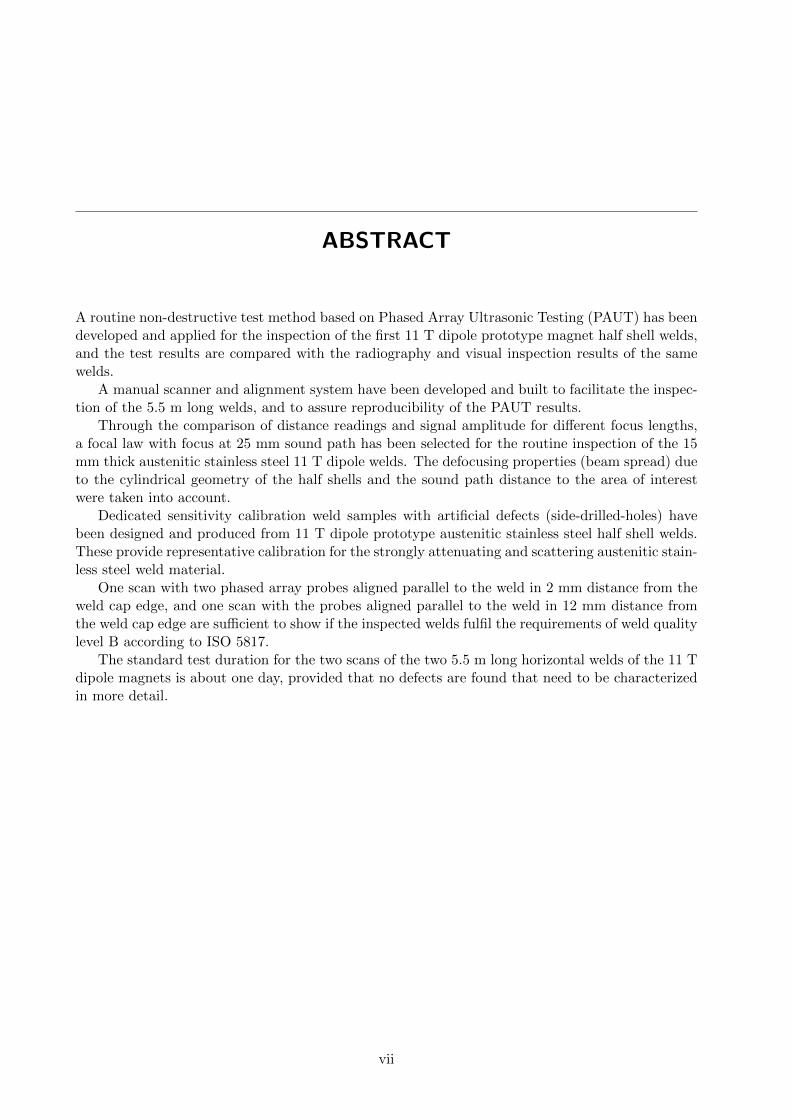
PAUT Phased Array Ultrasonic TestingDMA Dual Matrix ArrayCFU Couplant Feed UnitHAZ Heat-Affected-ZoneFSH Full-Screen-HeightSDH Side-Drilled-Hole: an artificially produced defect simulating volume defects
such as pores, inclusions, shrinkage cavity etc.FBH Flat-Bottomed-Hole: an artificially produced defect simulating flat defects
such as cracks and Lack-of-Fusion in the weld bevel.LOF Lack-Of-Fusion: an area of the weld which has not fused to the parent material.
Occurs typically at the weld bevel and between weld passes.
xi

CONTENTS
Abstract vii
Acknowledgements ix
Notation xi
1 Introduction 1
2 Theory 5
2.1 Basics of Ultrasonic Testing . . . . . . . . . . . . . . . . . . . . . . . . . . . . . . . . 5
2.2 Phased Array Ultrasonic Testing . . . . . . . . . . . . . . . . . . . . . . . . . . . . . 12
2.3 316LN Austenitic Stainless Steel . . . . . . . . . . . . . . . . . . . . . . . . . . . . . 17
3 Experimental Details 21
3.1 The Horizontal Welds of the 316LN Austenitic Stainless Steel Half Shells . . . . . . 21
3.2 PAUT Equipment . . . . . . . . . . . . . . . . . . . . . . . . . . . . . . . . . . . . . 24
3.3 Manual Scanner for Ultrasonic Testing of the Long Horizontal Welds of the 11 Tdipole . . . . . . . . . . . . . . . . . . . . . . . . . . . . . . . . . . . . . . . . . . . . 26
3.4 Calibration of the PAUT Set-Up . . . . . . . . . . . . . . . . . . . . . . . . . . . . . 27
3.5 Wedge-Surface Coupling to the Stainless Steel Shells and Required Surface Prepa-rations . . . . . . . . . . . . . . . . . . . . . . . . . . . . . . . . . . . . . . . . . . . . 31
3.6 Software . . . . . . . . . . . . . . . . . . . . . . . . . . . . . . . . . . . . . . . . . . . 32
3.7 Explanations of Views for Interpretation of PAUT data . . . . . . . . . . . . . . . . 32
4 Ultrasonic Beam Dynamics and Comparison of PAUT Focal Laws 37
4.1 The Effect of Structure of the Weld Material on Ultrasonic Beam Dynamics . . . . . 37
4.2 The Effect of the Stainless Steel Half Shells on Ultrasonic Beam Dynamics . . . . . . 41
4.3 Comparison of PAUT Focal Laws . . . . . . . . . . . . . . . . . . . . . . . . . . . . . 44
4.4 Discussion of the Results of Ultrasonic Beam Dynamics and Comparison of PAUTFocal Laws . . . . . . . . . . . . . . . . . . . . . . . . . . . . . . . . . . . . . . . . . 48
5 PAUT of the 11 T Dipole Magnet Welds 49
5.1 Results of Calibration and Reference Weld Samples . . . . . . . . . . . . . . . . . . 49
5.2 Results of the 11 T Dipole Prototype Magnet Horizontal Welds . . . . . . . . . . . . 59
5.3 Discussion of the Results of PAUT of the 11 T Dipole Magnet Welds . . . . . . . . . 66
6 Conclusion 69
xiii

xiv CONTENTS
Appendix A Weld Quality and Testing Requirements 73A.1 Quality Levels . . . . . . . . . . . . . . . . . . . . . . . . . . . . . . . . . . . . . . . . 73A.2 Acceptance Levels . . . . . . . . . . . . . . . . . . . . . . . . . . . . . . . . . . . . . 78A.3 Testing Techniques and Testing Level . . . . . . . . . . . . . . . . . . . . . . . . . . 80
Appendix B PAUT Equipment for 11 T Dipole Weld Inspection 83B.1 Main PAUT Equipment . . . . . . . . . . . . . . . . . . . . . . . . . . . . . . . . . . 83B.2 11 T Dipole Weld Calibration and Reference Samples . . . . . . . . . . . . . . . . . 85B.3 11 T Dipole Weld Samples . . . . . . . . . . . . . . . . . . . . . . . . . . . . . . . . . 86B.4 Other magnet austenitic stainless steel shell weld samples . . . . . . . . . . . . . . . 87B.5 16 mm Thick Austenitic Stainless Steel Flat Weld Sample . . . . . . . . . . . . . . . 87B.6 11 T Single Aperture Short Model Weld Samples . . . . . . . . . . . . . . . . . . . . 88B.7 Tools and Attachments . . . . . . . . . . . . . . . . . . . . . . . . . . . . . . . . . . . 88B.8 Miscellaneous Items . . . . . . . . . . . . . . . . . . . . . . . . . . . . . . . . . . . . 89
References 91
1
INTRODUCTION
CERN, the European Organization for Nuclear Research1, is the worlds largest particle physicslaboratory situated just outside Geneva, Switzerland. With over 10,000 visiting scientists, users,fellows and students representing over 600 universities from all over the world, the frontiers offundamental physics is being explored.
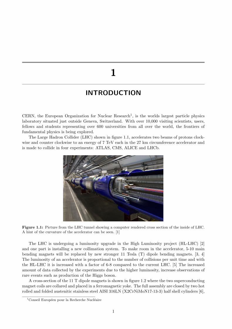
The Large Hadron Collider (LHC) shown in figure 1.1, accelerates two beams of protons clock-wise and counter clockwise to an energy of 7 TeV each in the 27 km circumference accelerator andis made to collide in four experiments: ATLAS, CMS, ALICE and LHCb.
Figure 1.1: Picture from the LHC tunnel showing a computer rendered cross section of the inside of LHC.A hint of the curvature of the accelerator can be seen. [1]
The LHC is undergoing a luminosity upgrade in the High Luminosity project (HL-LHC) [2]and one part is installing a new collimation system. To make room in the accelerator, 5-10 mainbending magnets will be replaced by new stronger 11 Tesla (T) dipole bending magnets. [3, 4]The luminosity of an accelerator is proportional to the number of collisions per unit time and withthe HL-LHC it is increased with a factor of 6-8 compared to the current LHC. [5] The increasedamount of data collected by the experiments due to the higher luminosity, increase observations ofrare events such as production of the Higgs boson.
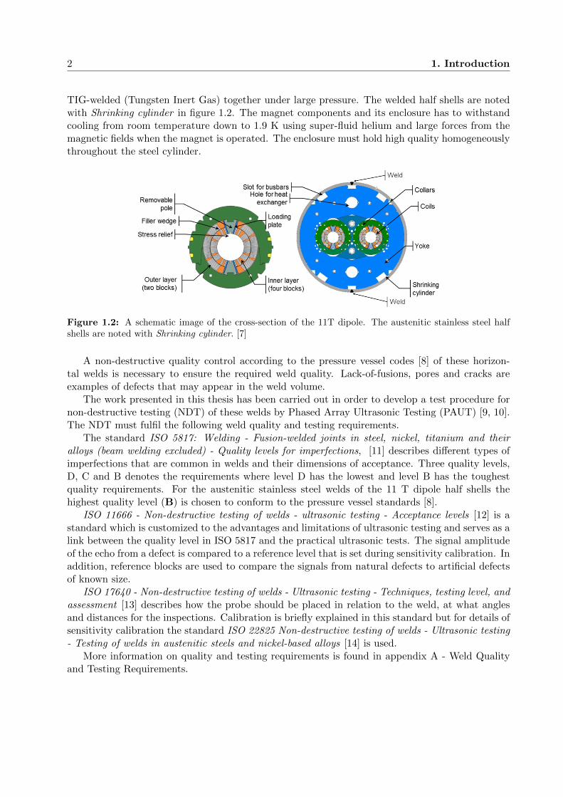
A cross-section of the 11 T dipole magnets is shown in figure 1.2 where the two superconductingmagnet coils are collared and placed in a ferromagnetic yoke. The full assembly are closed by two hotrolled and folded austenitic stainless steel AISI 316LN (X2CrNiMoN17-13-3) half shell cylinders [6],
1Conseil Europeen pour la Recherche Nucleaire
1
2 1. Introduction
TIG-welded (Tungsten Inert Gas) together under large pressure. The welded half shells are notedwith Shrinking cylinder in figure 1.2. The magnet components and its enclosure has to withstandcooling from room temperature down to 1.9 K using super-fluid helium and large forces from themagnetic fields when the magnet is operated. The enclosure must hold high quality homogeneouslythroughout the steel cylinder.
Figure 1.2: A schematic image of the cross-section of the 11T dipole. The austenitic stainless steel halfshells are noted with Shrinking cylinder. [7]
A non-destructive quality control according to the pressure vessel codes [8] of these horizon-tal welds is necessary to ensure the required weld quality. Lack-of-fusions, pores and cracks areexamples of defects that may appear in the weld volume.
The work presented in this thesis has been carried out in order to develop a test procedure fornon-destructive testing (NDT) of these welds by Phased Array Ultrasonic Testing (PAUT) [9, 10].The NDT must fulfil the following weld quality and testing requirements.
The standard ISO 5817: Welding - Fusion-welded joints in steel, nickel, titanium and theiralloys (beam welding excluded) - Quality levels for imperfections, [11] describes different types ofimperfections that are common in welds and their dimensions of acceptance. Three quality levels,D, C and B denotes the requirements where level D has the lowest and level B has the toughestquality requirements. For the austenitic stainless steel welds of the 11 T dipole half shells thehighest quality level (B) is chosen to conform to the pressure vessel standards [8].
ISO 11666 - Non-destructive testing of welds - ultrasonic testing - Acceptance levels [12] is astandard which is customized to the advantages and limitations of ultrasonic testing and serves as alink between the quality level in ISO 5817 and the practical ultrasonic tests. The signal amplitudeof the echo from a defect is compared to a reference level that is set during sensitivity calibration. Inaddition, reference blocks are used to compare the signals from natural defects to artificial defectsof known size.
ISO 17640 - Non-destructive testing of welds - Ultrasonic testing - Techniques, testing level, andassessment [13] describes how the probe should be placed in relation to the weld, at what anglesand distances for the inspections. Calibration is briefly explained in this standard but for details ofsensitivity calibration the standard ISO 22825 Non-destructive testing of welds - Ultrasonic testing- Testing of welds in austenitic steels and nickel-based alloys [14] is used.
More information on quality and testing requirements is found in appendix A - Weld Qualityand Testing Requirements.

3
The beam formation and propagation of ultrasound in the austenitic stainless steel weld cause alarge noise level but can be suppressed to acceptable levels using correct equipment and equipmentsettings. Water is used as coupling medium for the ultrasonic beam. To ensure a good coupling,the surface of the weld area is prepared before testing.
Longitudinal compression waves are used for the austenitic stainless steel. However only thefirst leg of the ultrasonic beam can be used with good certainty i.e. no skipping on the backwall. Because of the strong attenuation in the weld material and because of mode conversion fromlongitudinal waves to shear waves when the beam is skipped on the back wall, these signals canonly be used as an indicator of the presence of defects and is cause for further testing of the area.
The PAUT results are compared with radiography results of the same welds including detectabil-ity of different defects and a small discussion of the two methods advantages and disadvantages aregiven.

2
THEORY
2.1 Basics of Ultrasonic Testing
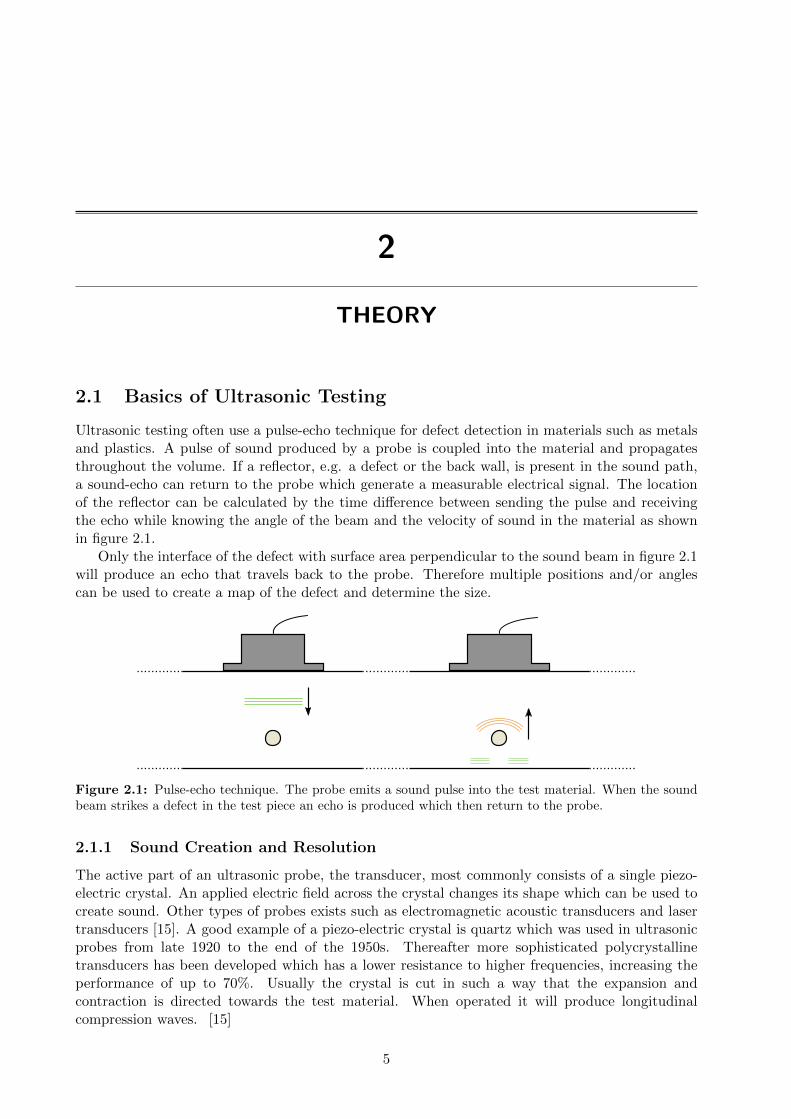
Ultrasonic testing often use a pulse-echo technique for defect detection in materials such as metalsand plastics. A pulse of sound produced by a probe is coupled into the material and propagatesthroughout the volume. If a reflector, e.g. a defect or the back wall, is present in the sound path,a sound-echo can return to the probe which generate a measurable electrical signal. The locationof the reflector can be calculated by the time difference between sending the pulse and receivingthe echo while knowing the angle of the beam and the velocity of sound in the material as shownin figure 2.1.
Only the interface of the defect with surface area perpendicular to the sound beam in figure 2.1will produce an echo that travels back to the probe. Therefore multiple positions and/or anglescan be used to create a map of the defect and determine the size.
Figure 2.1: Pulse-echo technique. The probe emits a sound pulse into the test material. When the soundbeam strikes a defect in the test piece an echo is produced which then return to the probe.
2.1.1 Sound Creation and Resolution
The active part of an ultrasonic probe, the transducer, most commonly consists of a single piezo-electric crystal. An applied electric field across the crystal changes its shape which can be used tocreate sound. Other types of probes exists such as electromagnetic acoustic transducers and lasertransducers [15]. A good example of a piezo-electric crystal is quartz which was used in ultrasonicprobes from late 1920 to the end of the 1950s. Thereafter more sophisticated polycrystallinetransducers has been developed which has a lower resistance to higher frequencies, increasing theperformance of up to 70%. Usually the crystal is cut in such a way that the expansion andcontraction is directed towards the test material. When operated it will produce longitudinalcompression waves. [15]
5

6 2. Theory
The pulse of sound is generated by applying a sharp electrical pulse to the piezo-electric crys-tal which then starts to oscillate at its own resonance frequency, fres, determined by the crystalthickness, tpiezo, and the compression wave velocity, Vpiezo, inside the piezo-crystal. By reducingthickness, the resonant frequency increase as described by equation 2.1, [15]. Typical useful fre-quencies for ultrasonic inspection range from 500 kHz to 20 MHz [16], and the diameter of thetransducer range from 6 mm to 13 mm, and even larger up to 25 mm in diameter for certainapplications. It should be noted that the crystal does not produce sound waves of only the exactresonant frequency. Rather it is a range of frequencies centred to the resonant frequency, called thebandwidth of the transducer.
fres =Vpiezo2tpiezo
(2.1)
The sound waves are coupled from the transducer into the test material using a liquid. Theatoms in the liquid start to oscillate at the same frequency as the crystal and eventually as thevibrations propagate they are coupled into the test material. It is important to have a low pulselength of the sound wave, i.e. to keep the number of resonant vibration periods low, typically1 to 5, because the pulse length determine the resolution of the inspection. For example twodefects close to each other as shown in figure 2.2. The time difference between the front and backof the pulses ∆t = t1 − t2, must be smaller than the time difference between reaching the twodifferent defects ∆T = T1 − T2. The pulse length, ∆t, can be calculated as the product betweennumber of periods, N, and wavelength, λ, in the material being inspected (∆t = N ∗ λ). Thepiezo-crystal of a conventional probe will normally have 12 or more periods depending on crystaldiameter and excitation method among others, which in most cases are too many. Therefore, byapplying a backing material on the backside of the crystal the number of periods is reduced throughdamping. [15, 9]
∆t = t1 − t2
∆T = T1 − T2
Figure 2.2: To distinguish between the two defects the relation: ∆t<∆T must be fulfilled.
2.1.2 Huygen’s Principle
According to Huygen’s principle, each point of an advancing wave-front acts as a point sourceof sound, emitting a new spherical wave. The resulting wave is the superposition of each of thesecondary waves. [9, 17] If the transducer is big compared to the wavelength, the result will bean almost straight beam. Nearly all of these ”point sources”, except the ones at the edges of thecrystal, will experience constructive interference only parallel to the path of propagation and forma uniform wave-front. However, if the transducer is small compared to the wavelength the resultwill become more of a spherical wave. A special case arise when using a rectangular transducerwhich can be considered big in one direction and small in the other and will therefore act as a linesource, creating cylindrical waves. This will become important in section 2.2.
2.1 Basics of Ultrasonic Testing 7
2.1.3 Modes of Propagation and Velocity
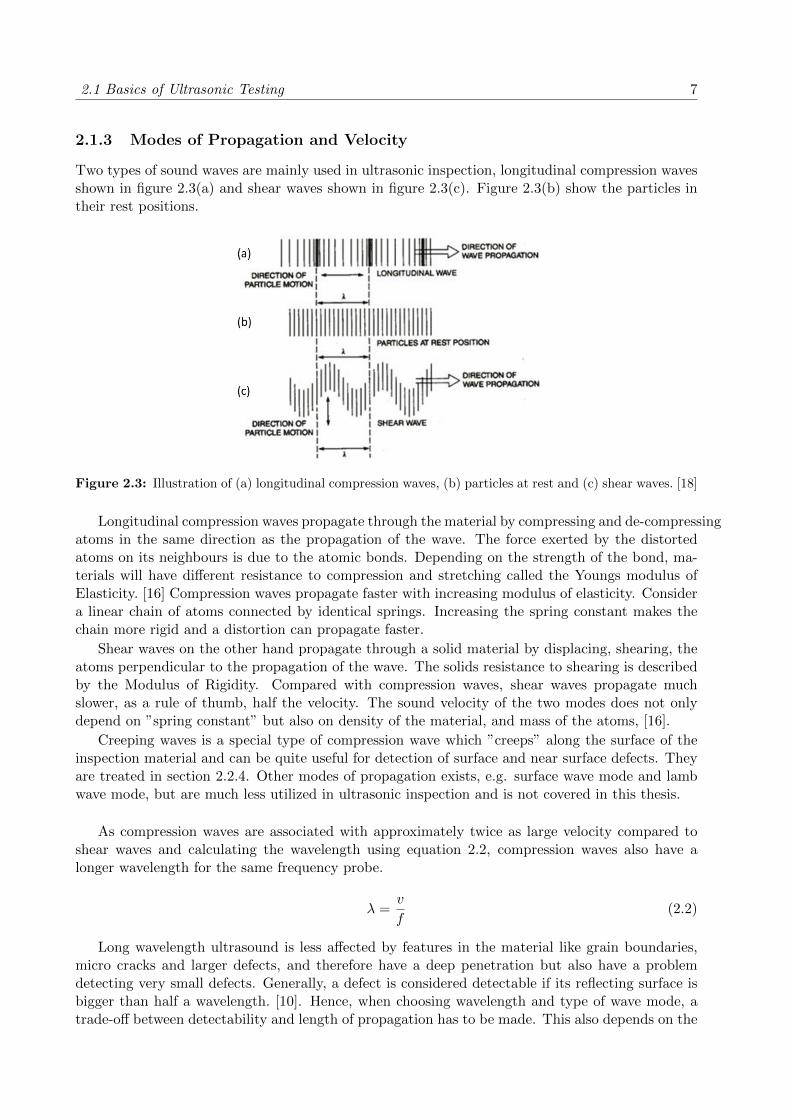
Two types of sound waves are mainly used in ultrasonic inspection, longitudinal compression wavesshown in figure 2.3(a) and shear waves shown in figure 2.3(c). Figure 2.3(b) show the particles intheir rest positions.
Figure 2.3: Illustration of (a) longitudinal compression waves, (b) particles at rest and (c) shear waves. [18]
Longitudinal compression waves propagate through the material by compressing and de-compressingatoms in the same direction as the propagation of the wave. The force exerted by the distortedatoms on its neighbours is due to the atomic bonds. Depending on the strength of the bond, ma-terials will have different resistance to compression and stretching called the Youngs modulus ofElasticity. [16] Compression waves propagate faster with increasing modulus of elasticity. Considera linear chain of atoms connected by identical springs. Increasing the spring constant makes thechain more rigid and a distortion can propagate faster.
Shear waves on the other hand propagate through a solid material by displacing, shearing, theatoms perpendicular to the propagation of the wave. The solids resistance to shearing is describedby the Modulus of Rigidity. Compared with compression waves, shear waves propagate muchslower, as a rule of thumb, half the velocity. The sound velocity of the two modes does not onlydepend on ”spring constant” but also on density of the material, and mass of the atoms, [16].
Creeping waves is a special type of compression wave which ”creeps” along the surface of theinspection material and can be quite useful for detection of surface and near surface defects. Theyare treated in section 2.2.4. Other modes of propagation exists, e.g. surface wave mode and lambwave mode, but are much less utilized in ultrasonic inspection and is not covered in this thesis.
As compression waves are associated with approximately twice as large velocity compared toshear waves and calculating the wavelength using equation 2.2, compression waves also have alonger wavelength for the same frequency probe.
λ =v
f(2.2)
Long wavelength ultrasound is less affected by features in the material like grain boundaries,micro cracks and larger defects, and therefore have a deep penetration but also have a problemdetecting very small defects. Generally, a defect is considered detectable if its reflecting surface isbigger than half a wavelength. [10]. Hence, when choosing wavelength and type of wave mode, atrade-off between detectability and length of propagation has to be made. This also depends on the

8 2. Theory
material to be inspected, some materials have large grains and many small features which result ina higher attenuation than others with small grains and few features.
2.1.4 Acoustical Coupling
Liquids and gases have no modulus of rigidity, therefore shear waves cannot propagate throughthem. They do however have a resistance to compression and stretching, i.e. elasticity, and thereforealso support compression waves! As mentioned earlier, ultrasound is coupled from the probe tothe inspected material using a liquid. The reason for this is to match the acoustical impedance,Zi, between probe and test piece. Equation 2.3 is used to calculate the percentage of reflectedsound energy, ER, when a wave encounters an interface between two materials, and is completelydetermined by the matching of the acoustical impedance. The percentage of transmitted sound,ET , is given by equation 2.4.
ER =
(Z1 − Z2
Z1 + Z2
)2
∗ 100% (2.3)
ET = 100%− ER (2.4)
where Z1 and Z2 are the impedances of material 1 and 2 respectively. The impedance miss-match between air (Z = 0.0004) and metal (Z = 44.8 for stainless steel) is very high meaningthat almost all energy is reflected. The miss-match between water (Z = 1.48) and stainless steelis much less but will still have an energy reflection of about 88%, meaning that only 12% of theenergy is usefully transmitted. Echoes returning from a defect experience the same reflection andtransmission, so only 12% of this is usefully transmitted back to the probe. In total, using the bestcouplant (e.g. glycerin) at optimal conditions, just above 2% of the energy will come back to theprobe. [19] If water is used as a couplant, the number is closer to 1.5%.
2.1.5 Snell’s Law and Mode Conversion
A sound beam incident on an interface of two materials with different sound velocities will bereflected and refracted according to Snells law, see equation 2.5.
sin(θi)
vi=
sin(θr)
vr=
sin(θR)
vR(2.5)
where θi, θr and θR are the incident, refracted and reflected beam angle respectively and vi, vrand vR the respective speed of sound in the material of propagation. A beam exiting a low velocityand entering a high velocity material, like wedge (plastic rexolite) to steel, will be refracted to agreater angle as shown in figure 2.4, and vice versa. Also, mode conversion takes place meaningthat an incident compression (C-wave) or shear wave (S-wave) will, at the interface, partly convertinto the opposite mode, both for the reflected and refracted beams. [20] Since compression andshear waves have different velocities they will be refracted and/or reflected at different angles. Forexample the shear wave is reflected at a smaller angle because it travels with about half the speedof sound compared to the compression wave. From here on it will be assumed that the incidentbeam is compression mode.

2.1 Basics of Ultrasonic Testing 9
Incident C-wave S-waveC-wave
C-wave
S-wave
Wedge
Steelθr,C
θr,S
θi,C
θR,S
θR,C
Figure 2.4: Snell’s law for a wedge (see section 2.2.3) to steel interface and incident C-wave. The reflectedC-wave has the same angle as the incident beam, but the mode converted S-wave reflection is at a smallerangle due to the lower velocity. The high velocity associated with C-waves in the steel cause a large refractionangle, but small for the slower S-wave.
Mode Conversion for Refraction
Parts of an incoming beam at a water-to-steel interface will, depending on the incident angle, berefracted and mode converted into shear waves. For low incidence angles in the water, the range of0◦-9◦, the percentage of mode conversion is small, i.e. an incoming compression wave will mostlyrefract in compression mode. But as the incidence angle is increased, a larger percentage of modeconversion takes place. At around 10◦ in the water, mode conversion is strong enough to convertshear waves with sufficient amplitude to give ”false” readings if a defect is present.
For an inspection with angled beams, a plastic wedge is commonly used, see section 2.2.3. Sincethe resulting beam angle in the sample, e.g. steel, is the same independent on choice of couplant,and only depends on the wedge angle, one can use the wedge angle as a reference. By using Snell’slaw to obtain the refraction angles for the interface between the wedge and couplant, e.g. water,(Eq. 2.6) and then for the interface between the couplant and the sample, e.g. steel, (Eq. 2.7) onecan eliminate the term for the couplant (Eq. 2.8).
sin(θwedge)
vwedge=
sin(θwater)
vwater(2.6)
sin(θwater)
vwater=
sin(θsteel)
vsteel(2.7)
=⇒sin(θwedge)
vwedge=
sin(θsteel)
vsteel(2.8)
Figure 2.5 illustrates mode conversion for different wedge angles. The first critical angle in aplastic rexolite wedge to steel interface is about 28◦ (15◦ for water) where the compression modewaves suffer total internal reflection. At larger angles only shear waves are transmitted. There isalso a second critical angle at 57◦ (28◦ for water) where not even shear waves can exist and iseventually mode converted into surface (Rayleigh) wave. [20]

10 2. Theory
Figure 2.5: Mode conversion of refraction for a compression wave probe for different incidence angles. Thex-axis is given in wedge angle, see 2.2.3. [9]
Mode Conversion for Reflection
The mode conversion for reflection is a bit different from refraction. If the incident beam travel ina liquid, typically a couplant between probe and test object, there can be no mode conversion intoshear waves since the liquid does not support shear waves. However, if there is an interface, e.g.steel to air in the form of a crack or a pore in a solid object, mode conversion for reflection canoccur. Low incidence angle compression waves produce reflections in mostly compression mode,but as the angle increases so does the mode converted shear wave until a maximum shear mode isreached as shown in figure 2.6(a).
Shear waves at low incidence angles will analogously reflect in shear mode. Increasing theincidence angle means increasing amount of compression mode waves as shown in figure 2.6(b). [20]
(a) Incident compression waves (b) Incident shear waves
Figure 2.6: (a) Mode conversion for reflection of an incident compression wave beam versus incidence angle.(b) Mode conversion for reflection of an incident shear wave beam versus incidence angle. [20]
2.1 Basics of Ultrasonic Testing 11
2.1.6 Attenuation and Beam characteristics
The energy loss when the sound beam is propagating through a material, i.e. attenuation, is causedby absorption, scattering, interference effects and beam spread [21].
Scattering and Absorption
Scattering depends on the size of the grains in the material where larger grains result in a largerscattering effect. This is because the grain boundaries of very large grains are wide and thereforeresult in a more prominent interface where reflection and refraction can occur. Absorption dependson the elastic properties of the material and is due to the movement of the atoms which continu-ously require energy. Longer wavelengths is less affected by the grain boundaries, and have lowerabsorption, so for a highly attenuating material one have to choose a probe with long wavelength,i.e. a low frequency. [21]
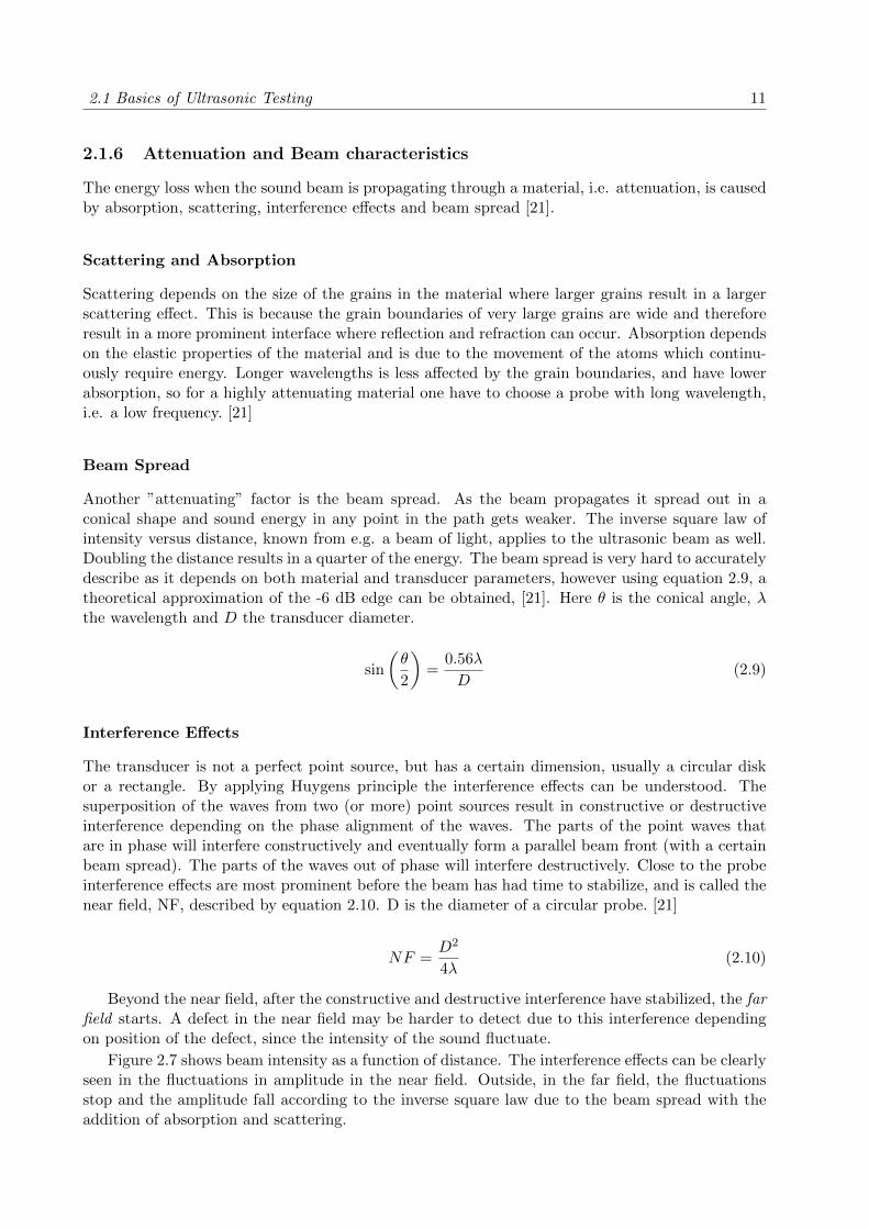
Beam Spread
Another ”attenuating” factor is the beam spread. As the beam propagates it spread out in aconical shape and sound energy in any point in the path gets weaker. The inverse square law ofintensity versus distance, known from e.g. a beam of light, applies to the ultrasonic beam as well.Doubling the distance results in a quarter of the energy. The beam spread is very hard to accuratelydescribe as it depends on both material and transducer parameters, however using equation 2.9, atheoretical approximation of the -6 dB edge can be obtained, [21]. Here θ is the conical angle, λthe wavelength and D the transducer diameter.
sin
(θ
2
)=
0.56λ
D(2.9)
Interference Effects
The transducer is not a perfect point source, but has a certain dimension, usually a circular diskor a rectangle. By applying Huygens principle the interference effects can be understood. Thesuperposition of the waves from two (or more) point sources result in constructive or destructiveinterference depending on the phase alignment of the waves. The parts of the point waves thatare in phase will interfere constructively and eventually form a parallel beam front (with a certainbeam spread). The parts of the waves out of phase will interfere destructively. Close to the probeinterference effects are most prominent before the beam has had time to stabilize, and is called thenear field, NF, described by equation 2.10. D is the diameter of a circular probe. [21]
NF =D2
4λ(2.10)
Beyond the near field, after the constructive and destructive interference have stabilized, the farfield starts. A defect in the near field may be harder to detect due to this interference dependingon position of the defect, since the intensity of the sound fluctuate.
Figure 2.7 shows beam intensity as a function of distance. The interference effects can be clearlyseen in the fluctuations in amplitude in the near field. Outside, in the far field, the fluctuationsstop and the amplitude fall according to the inverse square law due to the beam spread with theaddition of absorption and scattering.

12 2. Theory
Figure 2.7: The interference effects in the near field and the inverse square law in the far field. [9]
2.1.7 Focusing
Beam spread has a negative impact on the inspection sensitivity, where the sound energy is dispersedconically as shown in figure 2.8(a). However, using Huygens principle, shaping the transducerparabolic one can make the sound converge at a certain distance from the probe as shown infigure 2.8(b), maximizing the energy in that area. Described in section 2.1.4, the more energyat the defect, the stronger the returning signal. Since machining the transducer is permanent, aconventional focused probe can only be used in situations where the focus depth is matched to thetest object.
(a) (b)
Figure 2.8: (a) A conical beam from a conventional ultrasonic probe. (b) A focused beam from a conven-tional ultrasonic probe with parabolic transducer. [10]
2.2 Phased Array Ultrasonic Testing
The phased array probe basically consist of many small conventional ultrasonic probes packed inan array as shown in figure 2.9(a). The most common type is the linear array (1-D) which consistof several rectangular elements packed together with the long side towards each other. The small
2.2 Phased Array Ultrasonic Testing 13
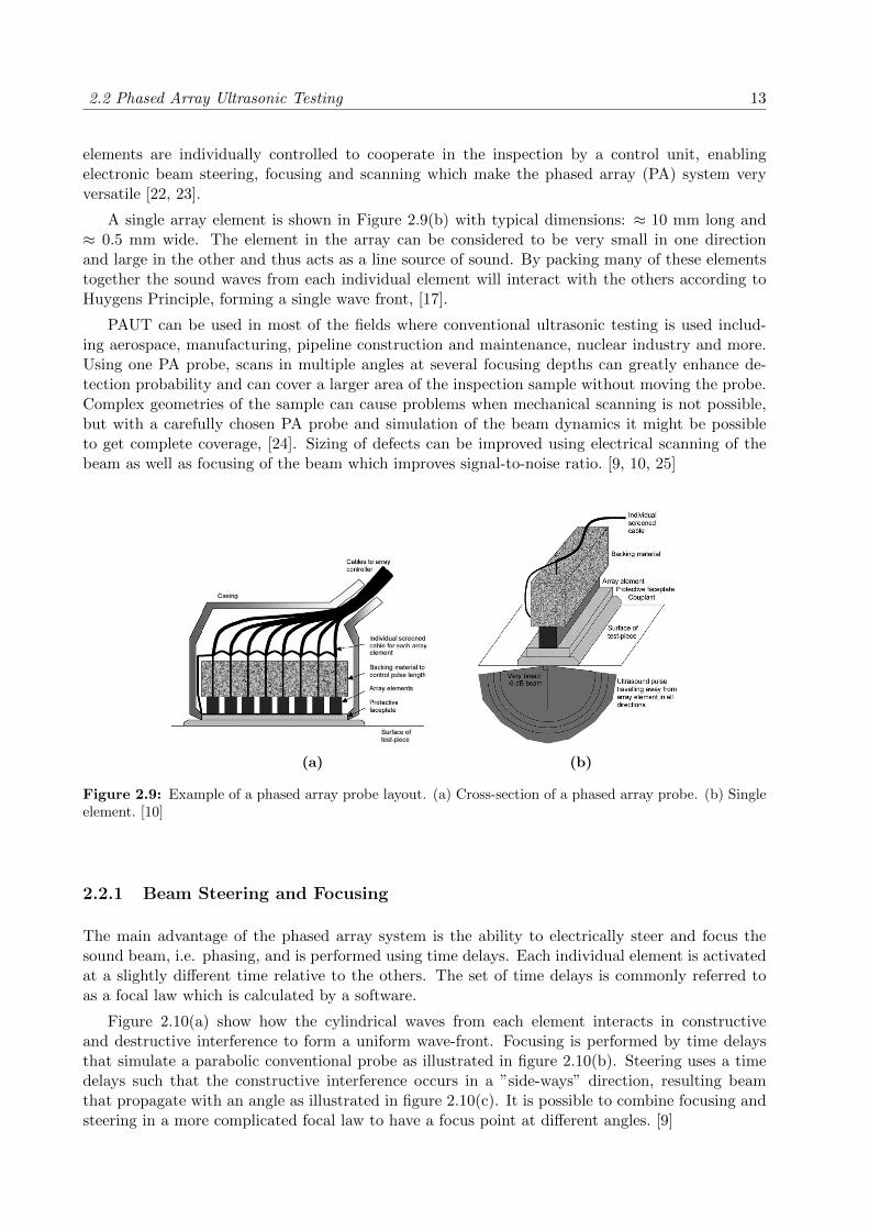
elements are individually controlled to cooperate in the inspection by a control unit, enablingelectronic beam steering, focusing and scanning which make the phased array (PA) system veryversatile [22, 23].
A single array element is shown in Figure 2.9(b) with typical dimensions: ≈ 10 mm long and≈ 0.5 mm wide. The element in the array can be considered to be very small in one directionand large in the other and thus acts as a line source of sound. By packing many of these elementstogether the sound waves from each individual element will interact with the others according toHuygens Principle, forming a single wave front, [17].
PAUT can be used in most of the fields where conventional ultrasonic testing is used includ-ing aerospace, manufacturing, pipeline construction and maintenance, nuclear industry and more.Using one PA probe, scans in multiple angles at several focusing depths can greatly enhance de-tection probability and can cover a larger area of the inspection sample without moving the probe.Complex geometries of the sample can cause problems when mechanical scanning is not possible,but with a carefully chosen PA probe and simulation of the beam dynamics it might be possibleto get complete coverage, [24]. Sizing of defects can be improved using electrical scanning of thebeam as well as focusing of the beam which improves signal-to-noise ratio. [9, 10, 25]
(a) (b)
Figure 2.9: Example of a phased array probe layout. (a) Cross-section of a phased array probe. (b) Singleelement. [10]
2.2.1 Beam Steering and Focusing
The main advantage of the phased array system is the ability to electrically steer and focus thesound beam, i.e. phasing, and is performed using time delays. Each individual element is activatedat a slightly different time relative to the others. The set of time delays is commonly referred toas a focal law which is calculated by a software.
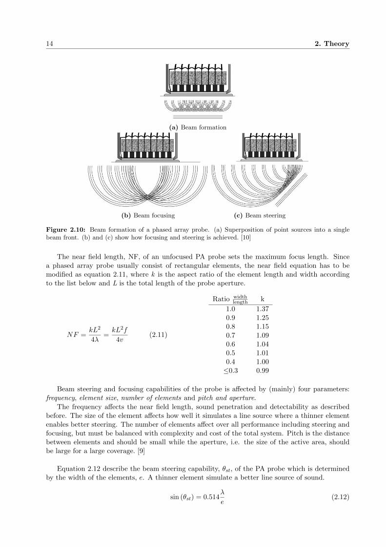
Figure 2.10(a) show how the cylindrical waves from each element interacts in constructiveand destructive interference to form a uniform wave-front. Focusing is performed by time delaysthat simulate a parabolic conventional probe as illustrated in figure 2.10(b). Steering uses a timedelays such that the constructive interference occurs in a ”side-ways” direction, resulting beamthat propagate with an angle as illustrated in figure 2.10(c). It is possible to combine focusing andsteering in a more complicated focal law to have a focus point at different angles. [9]
14 2. Theory
(a) Beam formation
(b) Beam focusing (c) Beam steering
Figure 2.10: Beam formation of a phased array probe. (a) Superposition of point sources into a singlebeam front. (b) and (c) show how focusing and steering is achieved. [10]
The near field length, NF, of an unfocused PA probe sets the maximum focus length. Sincea phased array probe usually consist of rectangular elements, the near field equation has to bemodified as equation 2.11, where k is the aspect ratio of the element length and width accordingto the list below and L is the total length of the probe aperture.
NF =kL2
4λ=kL2f
4v(2.11)
Ratio widthlength k
1.0 1.370.9 1.250.8 1.150.7 1.090.6 1.040.5 1.010.4 1.00≤0.3 0.99
Beam steering and focusing capabilities of the probe is affected by (mainly) four parameters:frequency, element size, number of elements and pitch and aperture.
The frequency affects the near field length, sound penetration and detectability as describedbefore. The size of the element affects how well it simulates a line source where a thinner elementenables better steering. The number of elements affect over all performance including steering andfocusing, but must be balanced with complexity and cost of the total system. Pitch is the distancebetween elements and should be small while the aperture, i.e. the size of the active area, shouldbe large for a large coverage. [9]
Equation 2.12 describe the beam steering capability, θst, of the PA probe which is determinedby the width of the elements, e. A thinner element simulate a better line source of sound.
sin (θst) = 0.514λ
e(2.12)

2.2 Phased Array Ultrasonic Testing 15
The versatility of the phased array probe enables the user to scan an area much faster thanwith conventional probes. By using a sequence of time delays in the focal law, refracted angles inthe sample from e.g. 40◦- 80◦ at an increment of 1◦ can be scanned simultaneously. And everyangle can have a different focus depth for maximum energy at the desired position. Compare withthe conventional probe which can scan only one angle at one focus depth.
2.2.2 Attenuation and Beam Spread
The sources of attenuation of the ultrasonic beam is the same for the phased array system as fora conventional probe. However the beam spread for rectangular elements depend on the lengthand width of the element and is described by equation 2.13. In the active steering plane, theelements are very small and therefore give a large beam spread, which is a wanted feature forelectronic steering. In the inactive plane however, the beam spread is small due to the relativelylong elements which is also a wanted feature! [9]
If the element width is too small, equation 2.13 becomes invalid, but the element will imitate aline source even better, which implies the beam spread is 180◦.
sinθb.sp
2=
0.44λ
L(2.13)
The width of the wave front in the inactive plane is considered approximately constant due tothe relatively long elements. Some beam spread occurs even for the long side of the element asseen in equation 2.14, but much less than for the short side of the element, equation 2.15. Theelement dimensions were taken as Llong = 10 mm and Lshort = 0.5 mm. Here λ = c/f = 1.45 mmfor stainless steel (c = 5800 m/s) and using a 4 MHz probe.
sinθb.sp
2=
0.44λ
Llong=
0.44 ∗ 1.45
10= 0.0638 −→ θb.sp = 7.32◦ (2.14)
sinθb.sp
2=
0.44λ
Lshort=
0.44 ∗ 1.45
0.5= 1.2760 −→ θb.sp = 180◦ (2.15)
2.2.3 Wedge
In many cases, especially for weld inspection, there is a need to use high angles, typically 40◦to90◦. Since the steering capabilities of a phased array system is limited, it poses a problem formany applications. By mounting the probe on a wedge one can set a mechanical starting anglefrom where the beam steering is offset to, illustrated in figure 2.11(b). When the probe is operatedwithout steering there is a relatively large angle of the sound in the test piece. From this new”zero” angle a range of e.g. 30◦to 90◦is possible. In addition the wedge acts as a protection for thesensitive probe surface from wear during the inspections.
Since the wedge is used for guiding the sound beam it is critical that the wedge parameters,e.g. geometry and speed of sound, are known so that the software know how to calculate the focallaws. For best results and best signal to noise ratio it is important that as much sound energy iscoupled into the test piece. The wedge should therefore have a very low attenuation and couplewell to the test piece, a common material is the plastic rexolite.

16 2. Theory
(a) (b)
Figure 2.11: (a) Example of a wedge, here with a probe (transmitter and receiver) mounted on top. (b)Illustration of the beam offset due to the angled wedge. [22]
2.2.4 Creeping Waves
Creeping waves can be seen as longitudinal compression waves that are refracted at very highangles, above 70◦ to 80◦, and propagate close to the surface of the test piece. They can thereforesuccessfully be used for sensitive detection of near surface defects. As the beam propagates, partsof the compression waves comes across the metal-air interface and thus continuously produce mode-converted shear waves, and can only be used for short distances. [26, 27]
Phased array probes that steer a beam above approximately 70◦ to 80◦ (using a wedge) willtherefore produce creeping waves. Because of the additional mode converted shear waves, a largernumber of reflected signals will most likely be received which can introduce interpretation difficul-ties. However, since the creeping waves travel with the same speed as the longitudinal compressionwaves, and shear waves travel with around half that speed, the signals from the creeping waves canoften be distinguished.
2.3 316LN Austenitic Stainless Steel 17
2.3 316LN Austenitic Stainless Steel
The half shell cylinders that encloses the 11 T dipole magnets are produced from 316LN austeniticstainless steel. Typical 316LN austenitic stainless steel material has an equiaxed homogeneous grainstructure, i.e. the shape of the grains. It has fairly small grains and no other phases or segregations.A chemical composition with large concentrations of Cr (16%-18%) and Ni (10%-14%) alloyed withFe form a stable austenitic phase in the 316 type stainless steel. Other alloying elements are alsoused, and traces of unwanted elements will be present that cannot be completely removed. [28]
The addition of N and Mo among others to a stainless steel Fe-Cr-Ni system, will furtherstabilize the austenitic phase, γ, such that precipitation of ferrite and martensite phase can befully eliminated. ”Nitrogen increases austenite stability against martensitic transformations and isa powerful austenite former with respect to ferrite. Nitrogen substantially increases strength, whileallowing ductility to be maintained down to cryogenic temperatures”. [29]
The completely austenitic phase of the half shells is required for many reason. For example, theaustenitic phase is non-magnetic is therefore well suited for a magnet enclosure, and it is unlikelyto crack when cooling to cryogenic temperatures. However, the process of welding in austeniticstainless steels changes the structure of the weld metal.
2.3.1 Grain structure of austenitic stainless steel welds
The result of welding in austenitic stainless steel depend on many variables such as welding process(Metal Inert Gas (MIG), Tungsten Inert Gas (TIG), electron beam...), choice of protection gas,heat input, additive material and welding speed to mention a few. [30, 31].
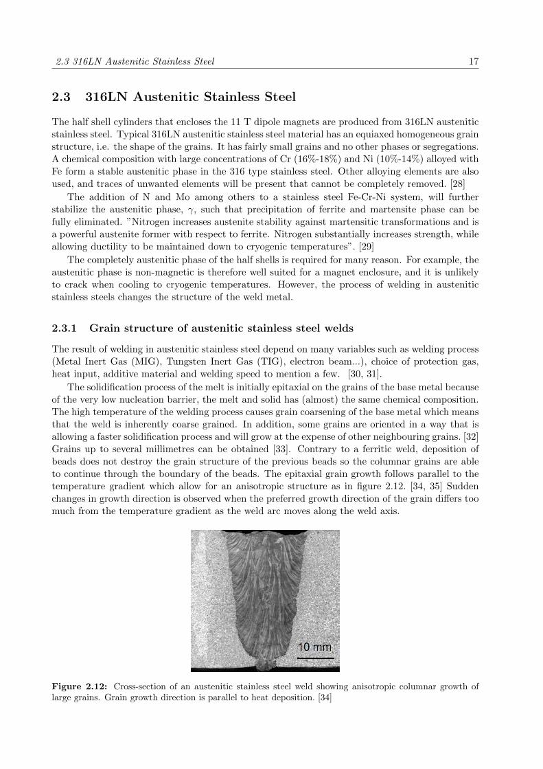
The solidification process of the melt is initially epitaxial on the grains of the base metal becauseof the very low nucleation barrier, the melt and solid has (almost) the same chemical composition.The high temperature of the welding process causes grain coarsening of the base metal which meansthat the weld is inherently coarse grained. In addition, some grains are oriented in a way that isallowing a faster solidification process and will grow at the expense of other neighbouring grains. [32]Grains up to several millimetres can be obtained [33]. Contrary to a ferritic weld, deposition ofbeads does not destroy the grain structure of the previous beads so the columnar grains are ableto continue through the boundary of the beads. The epitaxial grain growth follows parallel to thetemperature gradient which allow for an anisotropic structure as in figure 2.12. [34, 35] Suddenchanges in growth direction is observed when the preferred growth direction of the grain differs toomuch from the temperature gradient as the weld arc moves along the weld axis.
Figure 2.12: Cross-section of an austenitic stainless steel weld showing anisotropic columnar growth oflarge grains. Grain growth direction is parallel to heat deposition. [34]

18 2. Theory
The grains of the 316LN austenitic stainless steel weld material has a sub-grain microstructurewhich the parent material do not, shown in figure 2.13. Equiaxed, columnar and dendritic sub-grain structures is obtained [36]. The phase is still homogeneously austenitic, however an increasedamount of Cr and Mo is found in the sub-grain boundaries which induce lattice disorders such asdislocations. [37]
Figure 2.13: (a) SEM image showing the difference between the parent and weld metal of a 316LN austeniticstainless steel. (b) SEM image showing equiaxed sub-grain structure. (c) SEM image showing columnarsub-grain structure. (d) SEM image showing dendritic sub-grain structure. [36]
2.3.2 Precipitation of Other Phases in the Weld
In the weld solidification process the chemical composition of the melt can vary locally which canresult in precipitation of other phases than the face-centred-cubic, FCC, γ-austenite. [32] Body-centred-cubic, BCC, δ-ferrite has been observed to precipitate in between the γ dendrites in 316stainless steel, although in very small amounts. The chemical composition of the parent materialstrongly affect the composition of the melt and will determine the amount of δ-ferrite. For examplethe 304 type austenitic stainless steel is more susceptible to δ-ferrite precipitation in comparisonto the 316LN grade. [38, 39]
From δ-ferrite islands it is common to find transformed inter-metallic σ-phase which is ascribeda decreased corrosion resistance and degrading mechanical properties due to its bad coherence withaustenite and high interface energy. The σ-phase has a complex tetragonal structure and is veryhard and brittle. [38, 40, 41].
2.3.3 Formation of Macroscopic Defects
Many types of macroscopic weld defects (size in the order of millimetres) exist and their causesis manifold making it difficult to account for the origin of all of them. Defects such as incom-plete/excess root penetration, incorrect weld toe, overlap, burn through etc. (see appendix A) is

2.3 316LN Austenitic Stainless Steel 19
due to incorrect welding parameters such as too fast/slow welding speed, too little/much heat inputand incorrect amount of addition material. [42]
Pores and inclusions
Pores and inclusions are foreign material, gases and solids respectively, that is trapped inside theweld. While inclusions are intuitively understood as a foreign solid embedded in the weld, porosityhas multiple causes.
The protection gas shields the weld from the air which otherwise will oxidise the weld melt andcausing O and N to be trapped inside or react with the weld to form porosity. Each steel has anoptimum shielding gas composition which produce the highest quality weld for each application. [31]Small disturbances in the flow of shielding gas such as drafts in the room, too small or too largegas flow can cause air to reach the weld. Moisture or other contaminants such as paint, grease oroil is vaporized in the high welding temperature and disturbs the weld procedure which can causeporosity.
Cracks
316LN austenitic stainless steel has an excellent fracture resistance, but welding cause a significantdecrease in the resistance due to the sub-grain boundaries of the weld metal. An anisotropic fracturebehaviour has been observed, where the cracks prefer to propagate parallel to the dendritic structure[36]. Intermetallic σ phase embedded in the austenite matrix further weakens the weld metal andcan be the source of a crack.
Hot cracks can occur where cracks form in the solidification process and propagate through theweakened weld metal [43]. In addition, thermal shrinkage during cool-down and force impacts cancause cracking.
Lack-Of-Fusion
Lack-of-fusion is a part of the weld where the weld metal has not fused sufficiently to the basemetal, either at the weld bevel or at the previous weld pass in a multi-pass weld. They are likelyto occur when the weld arc is unable to raise the temperature to the melting point.
2.3.4 Sound Anisotropy and Large Attenuation of the Weld Material
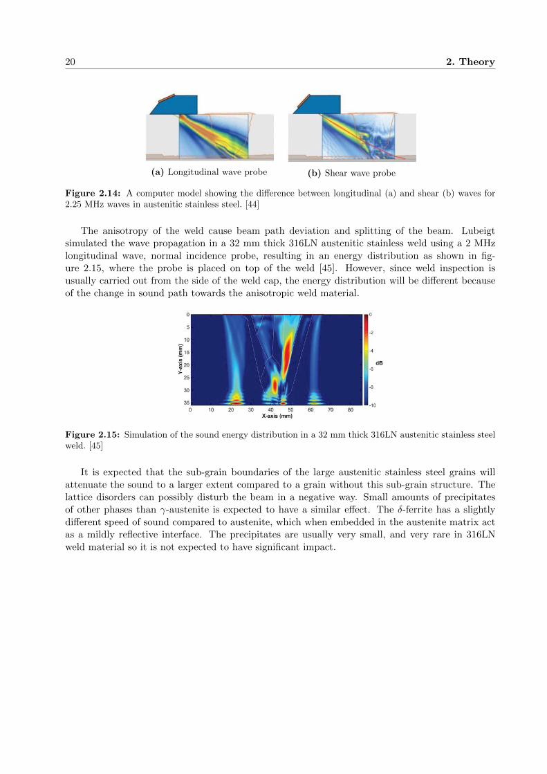
The large grained, anisotropic structure with columnar grains oriented parallel to the temperaturegradient has a big impact on the sound properties of the austenitic stainless steel weld metal. Shearwaves have been found to be affected more than longitudinal waves, resulting in high skewing andshort penetration depth as shown in figure 2.14. Therefore longitudinal waves are recommendedfor austenitic stainless steel. [44]
As the grains are comparably large to the wavelength of the sound, both in the order of 1mm, the grain boundary interfaces scatters the beam for a rather large beam spread. [34] Thisdeteriorate the signal to noise ratio because of the dispersed energy to a larger area. It also meansthat a larger area is covered which can cause a defect to appear in the wrong position or largerthan it normally would. [35]
The size of the defects are in the millimetre scale, i.e. the same scale as the actual grain size.Luckily the defect interfaces are much more reflective than the grain interfaces, and can produce alarge amplitude signal.
20 2. Theory
(a) Longitudinal wave probe (b) Shear wave probe
Figure 2.14: A computer model showing the difference between longitudinal (a) and shear (b) waves for2.25 MHz waves in austenitic stainless steel. [44]
The anisotropy of the weld cause beam path deviation and splitting of the beam. Lubeigtsimulated the wave propagation in a 32 mm thick 316LN austenitic stainless weld using a 2 MHzlongitudinal wave, normal incidence probe, resulting in an energy distribution as shown in fig-ure 2.15, where the probe is placed on top of the weld [45]. However, since weld inspection isusually carried out from the side of the weld cap, the energy distribution will be different becauseof the change in sound path towards the anisotropic weld material.
Figure 2.15: Simulation of the sound energy distribution in a 32 mm thick 316LN austenitic stainless steelweld. [45]
It is expected that the sub-grain boundaries of the large austenitic stainless steel grains willattenuate the sound to a larger extent compared to a grain without this sub-grain structure. Thelattice disorders can possibly disturb the beam in a negative way. Small amounts of precipitatesof other phases than γ-austenite is expected to have a similar effect. The δ-ferrite has a slightlydifferent speed of sound compared to austenite, which when embedded in the austenite matrix actas a mildly reflective interface. The precipitates are usually very small, and very rare in 316LNweld material so it is not expected to have significant impact.

3
EXPERIMENTAL DETAILS
3.1 The Horizontal Welds of the 316LN Austenitic Stainless SteelHalf Shells
The 5.5 m long HL-LHC 11 T dipole magnet coil assembly is closed by two 6.5 m long and 15 mmthick AISI 316LN (X2CrNiMoN17-13-3) austenitic stainless steel half shells [6] welded togetherunder large pre-pressure in an automated horizontal weld press, shown in figure 3.1. Both sides areTIG-welded simultaneously for a total of 13 passes, each pass taking ≈ 1 hour, depending on weldparameters. A 30mm×4mm backing plate placed behind the weld area keep the Ar protection gasfrom blowing away from the weld region when putting the first pass. After the horizontal weldsare finished ≈30 cm on each sides are cut away so the weld quality is not compromised from thestart and end of the weld passes.
Figure 3.1: Image of the welding procedure of the first 11 T dipole prototype magnet austenitic stainlesssteel half shells. The full magnet assembly is placed in a weld press with the pressure applied vertically andboth sides of the half shells welded simultaneously.
The pre-pressure created from the weld process is needed because of the thermal cycles themagnet is subjected to when cooling the magnet from room temperature to 1.9 K and back. Thedifferent thermal expansion coefficients of the magnet components can cause parts to move insidethe magnet if the pre-pressure is not large enough which will damage the sensitive superconducting
21
22 3. Experimental Details
coils. In operation, the large magnetic forces created in the two 11 T magnets can damage thesuperconducting cables if not fixed in their permanent positions.
A high quality austenitic stainless steel enclosure is needed to ensure that the magnet has a longoperation time. The weakest link is the welds which must be inspected non-destructively accordingto the standards of pressure vessels. [8]
The half shells are produced by ArcelorMittal according to CERN specifications [6], and followAISI 316LN or X2CrNiMoN17-13-3 according to EN 10028-7 [46] unless otherwise stated. Therequired chemical composition are shown in table 3.1. The physical and mechanical properties of thesteel, for example thermal contraction, relative magnetic permeability, tensile strength, weldabilityand machinability is all affected by the composition and this steel has been calculated to complywith the application requirements.
Table 3.1: Chemical composition of the 316LN austenitic stainless steel half shells. Concentration by mass%. Absolute concentration is given for one shell as an example. * CERN requirement. [6]
Element Concentration, % Limit, %
Chromium, Cr 18.0 *Min = 16.0; max = 18.0Nickel, Ni 12.7 *Min = 12; max = 14.0
Molybdenum, Mo 2.56 *Min = 2.00; max = 3.00Nitrogen, N 0.17 *Min = 0.15; max = 0.20
Carbon, C 0.03 Min = -; max = 0.03Silicon, Si 0.48 Min = -; max = 1.00
Manganese, Mn 1.19 Min = -; max = 2.00Cobalt, Co 0.02 Min = -; max = 0.10
Phosphor, P 0.016 *Min = -; max = 0.030Sulphur, S 0.001 *Min = -; max = 0.010
Iron, Fe 65 Remainder
The structure of the steel is completely homogeneous with only stable austenitic phase, no otherphases or segregations. It has a relative small grain size, the ASTM grain size number is higherthan 3 and homogeneous within ±1 throughout the shell. This is equivalent to a minimum of 62grains/mm2 calculated with equation: N = 15.5 ∗ 2G−1 where G is the grain size number. [47]
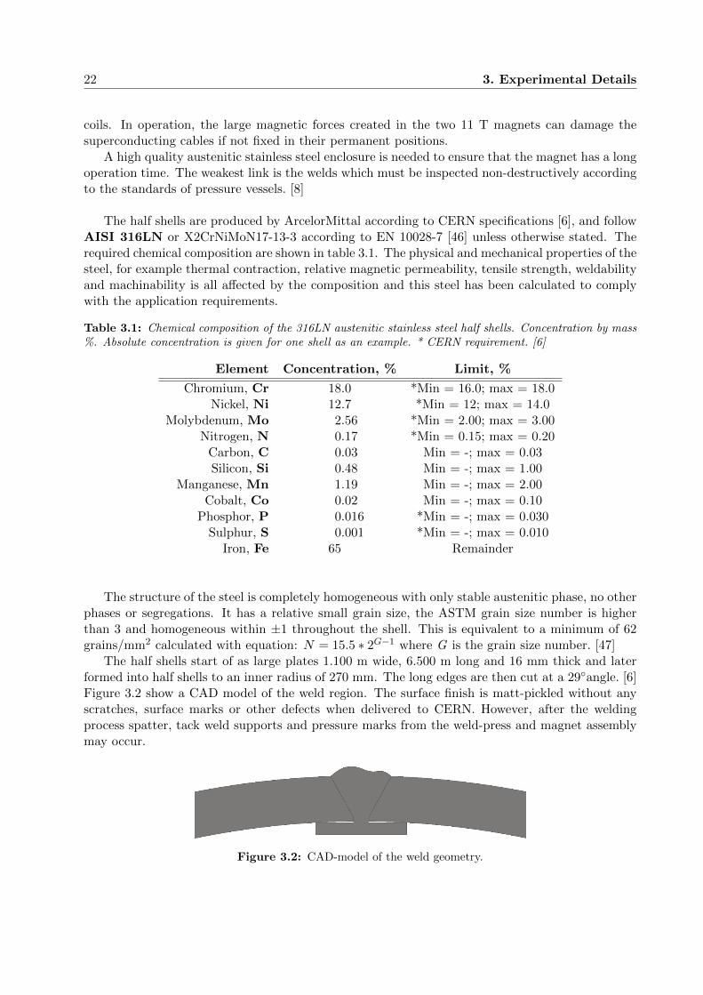
The half shells start of as large plates 1.100 m wide, 6.500 m long and 16 mm thick and laterformed into half shells to an inner radius of 270 mm. The long edges are then cut at a 29◦angle. [6]Figure 3.2 show a CAD model of the weld region. The surface finish is matt-pickled without anyscratches, surface marks or other defects when delivered to CERN. However, after the weldingprocess spatter, tack weld supports and pressure marks from the weld-press and magnet assemblymay occur.
Figure 3.2: CAD-model of the weld geometry.
3.1 The Horizontal Welds of the 316LN Austenitic Stainless Steel Half Shells 23
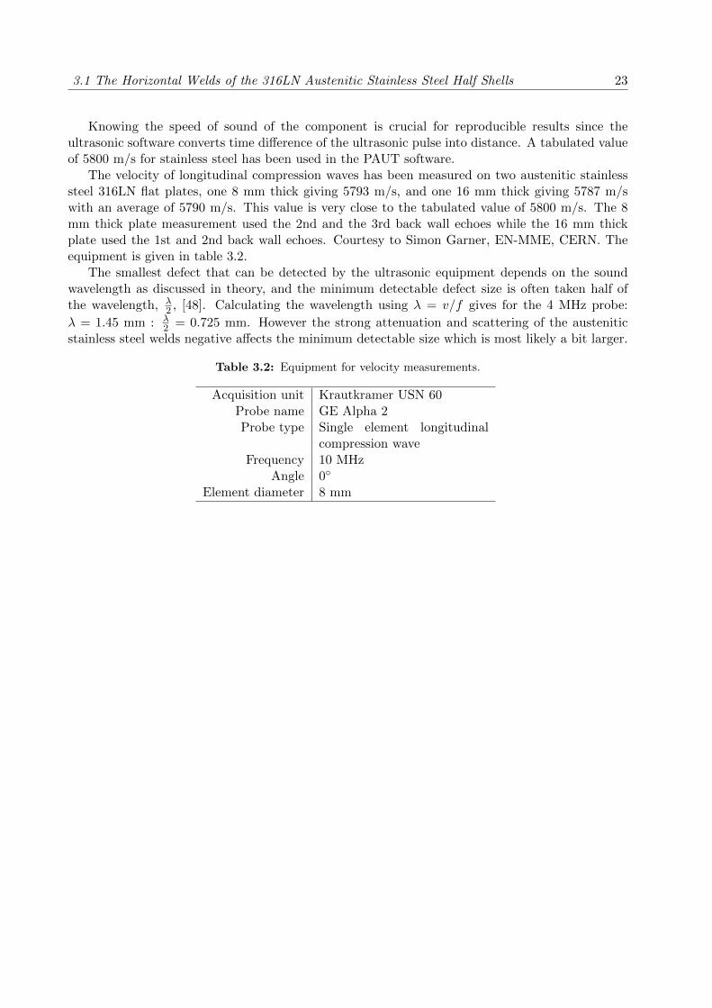
Knowing the speed of sound of the component is crucial for reproducible results since theultrasonic software converts time difference of the ultrasonic pulse into distance. A tabulated valueof 5800 m/s for stainless steel has been used in the PAUT software.
The velocity of longitudinal compression waves has been measured on two austenitic stainlesssteel 316LN flat plates, one 8 mm thick giving 5793 m/s, and one 16 mm thick giving 5787 m/swith an average of 5790 m/s. This value is very close to the tabulated value of 5800 m/s. The 8mm thick plate measurement used the 2nd and the 3rd back wall echoes while the 16 mm thickplate used the 1st and 2nd back wall echoes. Courtesy to Simon Garner, EN-MME, CERN. Theequipment is given in table 3.2.
The smallest defect that can be detected by the ultrasonic equipment depends on the soundwavelength as discussed in theory, and the minimum detectable defect size is often taken half ofthe wavelength, λ
2 , [48]. Calculating the wavelength using λ = v/f gives for the 4 MHz probe:
λ = 1.45 mm : λ2 = 0.725 mm. However the strong attenuation and scattering of the austenitic
stainless steel welds negative affects the minimum detectable size which is most likely a bit larger.
Table 3.2: Equipment for velocity measurements.
Acquisition unit Krautkramer USN 60Probe name GE Alpha 2Probe type Single element longitudinal
compression waveFrequency 10 MHz
Angle 0◦
Element diameter 8 mm

24 3. Experimental Details
3.2 PAUT Equipment
The essential PAUT components are the acquisition unit, the probes with wedges and the en-coder for position measurement. A full list of the PAUT equipment can be found in appendix B- PAUT Equipment for 11 T Dipole Weld Inspection. The PAUT unit Omniscan MX2 fromOlympus is shown in figure 3.3. The acquisition/control unit OMNI-M2-PA 32:128PR capableof simultaneous and individual control of 32 elements, with support for 128 channels. A splitter,Omni-A2-SPLIT128, is used to be able to connect two probes for a two side inspection set-up.The longitudinal 4 MHz Dual-Matrix-Array, DMA, probes Olympus DMA-4M-16X2-A27 that areshown in figure 3.4(c), contain a transmitter and a receiver in separate housings. The longitudi-nal DMA wedges SA27-DN55L-FD15-IHC, (figure 3.4(b)), have a sound insulating barrier in themiddle so that the transmitter and receiver probes are acoustically insulated, which minimizes theacoustic feedback. The Olympus Mini-Wheel encoder, (figure 3.4(d)), is capable of recording 12steps/mm.
Figure 3.3: Omniscan MX2 acquisition unit.
(a) (b)
(c) (d)
Figure 3.4: (a) Probe and wedge assembly. (b) Wedge Olympus SA27-DN55L-FD15-IHC, (c) dual matrixarray probes Olympus DMA-4M-16X2-A27 and (d) encoder for PAUT testing of the 11 T dipole shells.

3.2 PAUT Equipment 25
The 4 MHz longitudinal wave dual matrix probes DMA-4M-16X2-A27 have been selected be-cause of their good penetration depth in large grained austenitic stainless steel welds and theirrelatively good sensitivity for small sized defects. The splitting of the probe into one transmitterand one receiver, called the transmit-receive longitudinal (TRL) technique, gives an improved signalto noise ratio. ”These probes eliminate the interface echo, have no dead zones due to wedge echoes,reduce the backscattering signals and permit the use of higher gain”, [49]. The TRL technique isespecially used for acoustically noisy materials such as austenitic stainless steel welds and dissimilarweld material.
Wedges with an 18.7◦ wedge angle are used in order to offset the beam to around 55◦ in the steelmaterial, as described in the theory section (figure 2.11(b)), so that it can enter the weld region.With the additional mechanical 55◦ offset, the electronic beam steering can reach angles betweenapproximately 30◦ to 85◦. The wedges are custom made for the TRL DMA probes with a soundinsulating barrier to isolate the transmitter from the receiver parts. The two probe housings arethen placed on the wedge which has a small roof angle that creates a pseudo-focused beam, i.e. thereceiver is only sensitive for signals from a limited volume where two beams from the transmitterand receiver overlap as shown in figure 3.5. [44]
Figure 3.5: The TRL technique. [44]
Probe: DMA-4M-16X2-A27 Wedge: SA27-DN55L-FD15-IHC• Dual matrix array, DMA • Longitudinal DMA wedge• Longitudinal waves • Wedge angle: 18.7◦
• Frequency: 4MHz • Roof angle: 3.7◦
• Element count: 64 • Material: Rexolite• Active area: Length 16 mm, elevation 6 mm • Nominal beam angle: 55◦
• Primary pitch: 1.0 mm • Bottom surface: Flat• Secondary pitch: 3.0 mm • Irrigation ports for water couplant• Matching medium: Rexolite • Carbides for wear protection
For the active area, 16 mm×6 mm, and the width of the element, ≈1 mm, the near field distanceis: N = 0.99∗162
4∗1.45 ≈ 44mm using equation 2.11 with aspect ratio k = 0.99 and λ = cf = 5800m/s
4MHz =1.45mm
The beam steering capability is: θst = arcsin(0.514 ∗ 1.45
1
)≈ 48.2◦ using equation 2.12
Beam spread in the inactive plane of the probe is calculated using equation 2.13:θb.sp = 2 ∗ arcsin
(0.44∗1.45
6
)≈ 12.2◦
The encoder Mini-Wheel shown in figure 3.4(d), from Olympus is connected to the Omniscanto synchronize the probe movement with data acquisition in the scan axis at 12 steps/mm. Thisenables the user to position and dimension indications found in the weld. The encoder attachment

26 3. Experimental Details
is spring loaded to keep it in contact with the rolling surface at all times.
A couplant feed unit from Olympus, CFU05, was acquired to supply water couplant to thewedges. The pump is a diaphragm type to avoid priming problems and has a bypass to ensureconstant water flow. The maximum flow capacity is 3.78 L/min, and adjustable through a controlvalve. The water inlet tube is equipped with a check valve to make sure it is always filled, an algaefilter and a debris filter. [50]
3.3 Manual Scanner for Ultrasonic Testing of the Long HorizontalWelds of the 11 T dipole
A mechanical scanner for PAUT testing of the horizontal welds of the 11 T dipole half shells has beendeveloped and was produced in the Large Magnet Facility (LMF) workshop at CERN. Figure 3.6(a)shows the scanner placed on top of the first 11 T dipole prototype magnet. Figure 3.6(b) show aCAD assembly of the scanner.
(a) (b)
Figure 3.6: (a) 11 T dipole prototype magnet weld with PAUT set-up. (b) CAD assembly of the scanneron top of magnet half shells. A mounted T-bar is also shown.
The scanner allows to guide two DMA probes along either side of the weld. An alignmentsystem, two adjustable wedge holders, a length position encoder, coupling water supply and cableholders are integrated in the scanner for easier operation.
The frame was built with aluminium profiles for good mechanical stability and offers to addparts in the future. The wheels, handles, hinges, tubes and other small parts were bought off theshelf. Custom parts, e.g. the wedge holders, were produced in-house.
The scanner is aligned to the weld by a T-bar that is mounted on top of the weld using speciallydesigned T-bar holders and clamps see appendix B, figure B.1. Four wheels, two on each side withrolling direction in the horizontal plane is pressing towards the T-bar with spring loaded hinges asshown in figure 3.6(b). This means that the probes will have a constant distance to the T-bar atall times.
The wedges are mounted on spring loaded linear gliders to keep the wedge pressed to the halfshell surface during the entire scan, shown in figure 3.7. The wedge holders have multiple degreesof freedom in order to align probe height, vertical distance and angle with respect to the weld.

3.4 Calibration of the PAUT Set-Up 27
(a) (b)
Figure 3.7: (a) Top view of the wedge holder with mounted wedge. (b) Front view of the wedge holder.Arrows show axis of motion.
3.4 Calibration of the PAUT Set-Up
The primary purpose of the PAUT set-up calibration is to be able to draw quantitative conclusionsof the position, the size and the type of defects that are causing an echo in the PAUT inspectiondata. By using dedicated calibration blocks with different artificial defects, the gain of the reflectedsignal can be adjusted in a way that same sized defects give a similar response independent ofdefect location.
3.4.1 Range Calibration
Before range calibration the beam exit point from the wedge must be determined. The beam exitpoint is defined as the point on the bottom of the wedge where the most energy exits the wedge, i.e.at the centre of the beam. A phased array probe has a range of beam exit points, approximately2 mm, depending on the different angles of the beams. In this note the 55◦ beam was chosen fordetermining beam exit point since this is the wedge offset angle.
Calibration block No 2 (figure 3.8(a)) has been used for beam exit point and range calibrationas described in ISO 7963 - Welds in steel - Calibration block No. 2 for ultrasonic examination ofwelds [52]. The beam exit point for the 55◦ beam is found by placing the probe facing the 25 mmradius and maximizing the signal from the (1st) back wall echo shown in figure 3.8(b). Section 3.7describes how to interpret the data in figure 3.8(b). The exit of the centre of the beam energynow coincide with the centre of the 25 mm radius back wall. The sound path distance measuredby the instrument should show 25 mm, although that is rarely the case before calibration. Smalldifferences in wedge dimensions will show up as range deviations. Therefore a wedge delay ismanually set until the echo align with 25mm.
The echoes in the angular range deviate slightly from the 25 mm sound path as shown infigure 3.8(b). This is because of the different beam exit points for higher and lower angle beams.By applying an angle dependent wedge delay, more for large angles and less for low angles thePAUT equipment can compensate for the different beam exit points so all angles show 25±1 mmsound path.

28 3. Experimental Details
To control the quality of the range calibration a measurement on the 50 mm radius on block No.2 shall be performed routinely before starting the 11 T dipole weld inspection. Measuring on otheraustenitic stainless steel blocks with known artificial defects can be used to verify the calibrationas well.
(a) (b)
Figure 3.8: (a) Probe and wedge positioned on the calibration block No. 2. (b) A- and S-scan of the backwall echo from the 25 mm radius of calibration block No. 2.
3.4.2 Sensitivity Calibration
Typically, two types of sensitivity calibrations are required, Angle-Corrected-Gain (ACG) andTime-Corrected-Gain (TCG). The ACG is very important and will determine detectability andsizing of defects. TCG on the other hand is not required in this project because the sound pathdistances to the areas of interest in the relatively thin 15 mm half shell welds are similar, between20 and 30 mm. Therefore, unless explicitly mentioned, all PAUT results presented in this notehave been acquired with ACG but not with TCG.
Two defects of the same type, size and distance to the beam exit point will not give the sameamplitude response depending on the needed beam angle to reach them. The increased beamspread, mode conversion, attenuation and scattering associated with high angle beams result in aweak signal. The ACG apply an angle dependent gain to bring the signals of defects of the samesize and type from all angles to the same amplitude.
An ACG can be constructed by two different methods. One method is by directly adjustingthe gain while measuring on a block with a radius, like on calibration block No.2. The amplituderecorded for each angle is corrected by the machine to show e.g. 80% full-screen-height, FSH.
The other method is by recording the amplitude from two or three artificial defects at the samesound path but reached by different angled beams. The signals received from these defects arecorrected to show e.g. 80% FSH. Based on the corrected gain for these two or three angles themachine extrapolates a correction gain for all other angles.
The last method offers more flexibility. The choice of artificial defect type and size will affectthe calibration. A good representative calibration is obtained with a block with artificial defectsproduced from a weld material. The best calibration is obtained if the block is an exact replica ofthe material intended for the inspection. Therefore, calibration blocks has been produced from thecut-off end welds of the 11 T dipole prototype magnet.
The highly attenuating and anisotropic austenitic stainless steel weld material and the curvedshell surface of the 11 T dipole magnet will affect the ultrasonic beam propagation in an oftenunexpected manner. By machining side-drilled-holes (SDHs) in the weld material these can beused to directly measure the received amplitudes and that way estimate the ultrasonic propertiesfor the ACG. A CAD model of a weld sample with SDHs in the weld centreline is shown infigure 3.9(a) and a reference sample with SDHs in the fusion line is shown in figure 3.9(b). Similar

3.4 Calibration of the PAUT Set-Up 29
weld samples with notches in the surfaces, flat-bottomed-holes (FBHs) drilled to the fusion lineand SDHs at different positions can be used as references for sizing and positioning of defects.
(a) Centreline (b) Fusion line
Figure 3.9: (a) CAD model of a sample with centreline SDHs. (b) CAD model of a sample with fusionline SDHs.
3.4.3 Calibration Station
A good calibration of the ultrasonic testing system is needed for a quantitative defect analysis.Again, the mechanical stability and position of the probes in regard to the weld of the blocks are ofhighest importance. As described in ISO 17640 [13] the system must be calibrated before and afterevery test and if any changes in configuration is made. Therefore, the calibration station shown infigure 3.10 was designed and produced to facilitate routine sensitivity calibrations prior to the 11T dipole weld inspections.
The purpose of the station is to simulate the magnet inspection while using calibration blockswith known and defined artificial defects. The blocks are placed on the red rubber covered tubesand aligned to the T-bar. After calibration the probe and wedges can remain mounted in thescanner while it is removed. This way the probe-weld distance and probe angle in relation to theweld can be maintained for representative calibration.
Figure 3.10: The calibration station with scanner. The calibration blocks are placed on the red tubes, theT-bar is used to align the scanner to the welds of the samples. The rails keep the scanner in the correctheight position.
3.4.4 Stainless Steel Welds from 11 T Dipole with Artificial Defects for Cali-bration and Reference measurements
From the 15 mm thick 316LN austenitic stainless steel half shell welds that were cut from theextending ends of the first 11 T dipole prototype magnet half shells, four representative calibrationand reference samples with artificial defects could be produced. Their design follow ISO 22825 [14].
30 3. Experimental Details
In order to exclude the presence of large natural defects, and to confirm the position of theartificial defects (SDHs, FBHs and notches), the weld samples were examined by radiography,which did not reveal any natural defects.
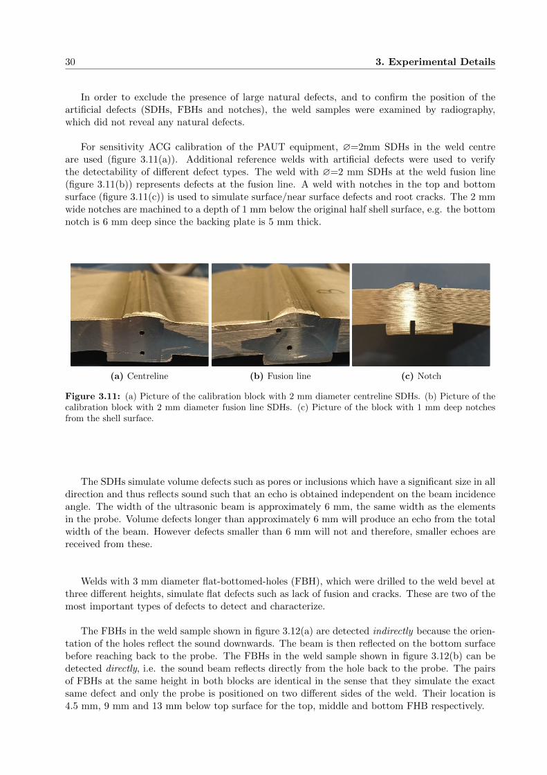
For sensitivity ACG calibration of the PAUT equipment, ∅=2mm SDHs in the weld centreare used (figure 3.11(a)). Additional reference welds with artificial defects were used to verifythe detectability of different defect types. The weld with ∅=2 mm SDHs at the weld fusion line(figure 3.11(b)) represents defects at the fusion line. A weld with notches in the top and bottomsurface (figure 3.11(c)) is used to simulate surface/near surface defects and root cracks. The 2 mmwide notches are machined to a depth of 1 mm below the original half shell surface, e.g. the bottomnotch is 6 mm deep since the backing plate is 5 mm thick.
(a) Centreline (b) Fusion line (c) Notch
Figure 3.11: (a) Picture of the calibration block with 2 mm diameter centreline SDHs. (b) Picture of thecalibration block with 2 mm diameter fusion line SDHs. (c) Picture of the block with 1 mm deep notchesfrom the shell surface.
The SDHs simulate volume defects such as pores or inclusions which have a significant size in alldirection and thus reflects sound such that an echo is obtained independent on the beam incidenceangle. The width of the ultrasonic beam is approximately 6 mm, the same width as the elementsin the probe. Volume defects longer than approximately 6 mm will produce an echo from the totalwidth of the beam. However defects smaller than 6 mm will not and therefore, smaller echoes arereceived from these.
Welds with 3 mm diameter flat-bottomed-holes (FBH), which were drilled to the weld bevel atthree different heights, simulate flat defects such as lack of fusion and cracks. These are two of themost important types of defects to detect and characterize.
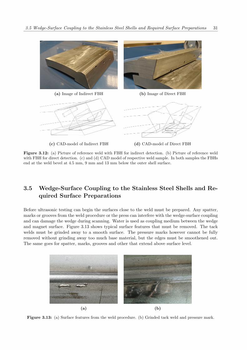
The FBHs in the weld sample shown in figure 3.12(a) are detected indirectly because the orien-tation of the holes reflect the sound downwards. The beam is then reflected on the bottom surfacebefore reaching back to the probe. The FBHs in the weld sample shown in figure 3.12(b) can bedetected directly, i.e. the sound beam reflects directly from the hole back to the probe. The pairsof FBHs at the same height in both blocks are identical in the sense that they simulate the exactsame defect and only the probe is positioned on two different sides of the weld. Their location is4.5 mm, 9 mm and 13 mm below top surface for the top, middle and bottom FHB respectively.
3.5 Wedge-Surface Coupling to the Stainless Steel Shells and Required Surface Preparations 31
(a) Image of Indirect FBH (b) Image of Direct FBH
(c) CAD-model of Indirect FBH (d) CAD-model of Direct FBH
Figure 3.12: (a) Picture of reference weld with FBH for indirect detection. (b) Picture of reference weldwith FBH for direct detection. (c) and (d) CAD model of respective weld sample. In both samples the FBHsend at the weld bevel at 4.5 mm, 9 mm and 13 mm below the outer shell surface.
3.5 Wedge-Surface Coupling to the Stainless Steel Shells and Re-quired Surface Preparations
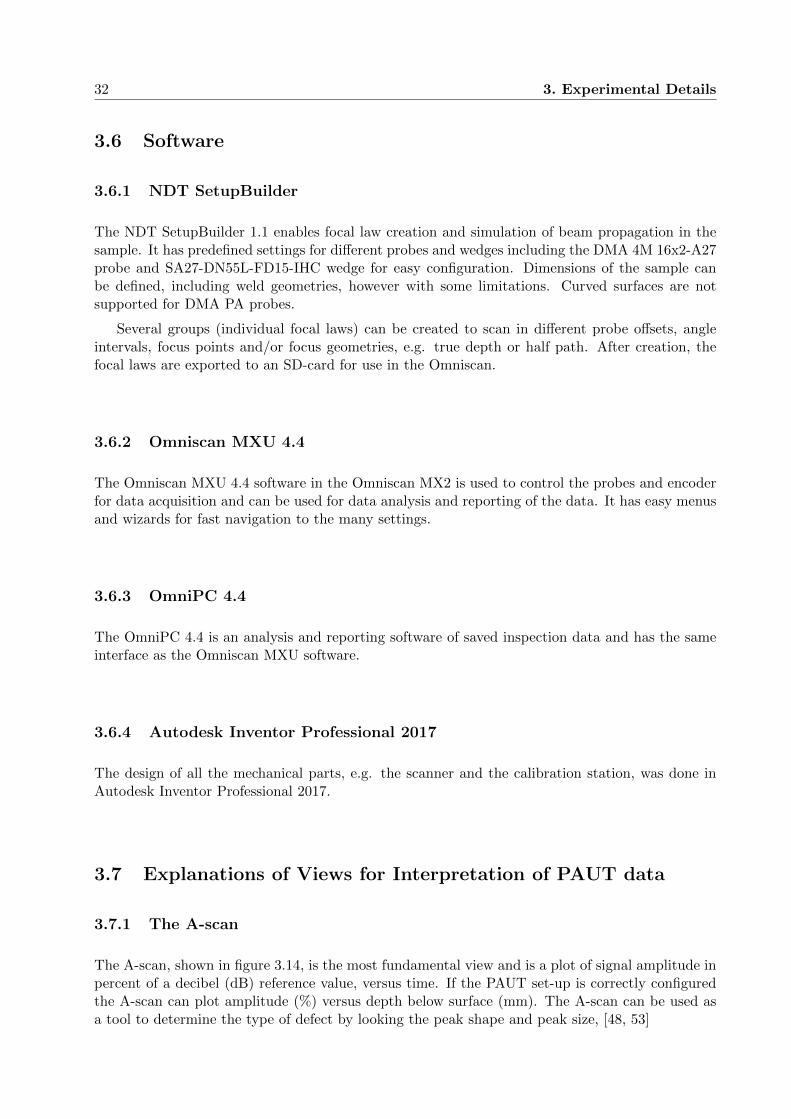
Before ultrasonic testing can begin the surfaces close to the weld must be prepared. Any spatter,marks or grooves from the weld procedure or the press can interfere with the wedge-surface couplingand can damage the wedge during scanning. Water is used as coupling medium between the wedgeand magnet surface. Figure 3.13 shows typical surface features that must be removed. The tackwelds must be grinded away to a smooth surface. The pressure marks however cannot be fullyremoved without grinding away too much base material, but the edges must be smoothened out.The same goes for spatter, marks, grooves and other that extend above surface level.
(a) (b)
Figure 3.13: (a) Surface features from the weld procedure. (b) Grinded tack weld and pressure mark.
32 3. Experimental Details
3.6 Software
3.6.1 NDT SetupBuilder
The NDT SetupBuilder 1.1 enables focal law creation and simulation of beam propagation in thesample. It has predefined settings for different probes and wedges including the DMA 4M 16x2-A27probe and SA27-DN55L-FD15-IHC wedge for easy configuration. Dimensions of the sample canbe defined, including weld geometries, however with some limitations. Curved surfaces are notsupported for DMA PA probes.
Several groups (individual focal laws) can be created to scan in different probe offsets, angleintervals, focus points and/or focus geometries, e.g. true depth or half path. After creation, thefocal laws are exported to an SD-card for use in the Omniscan.
3.6.2 Omniscan MXU 4.4
The Omniscan MXU 4.4 software in the Omniscan MX2 is used to control the probes and encoderfor data acquisition and can be used for data analysis and reporting of the data. It has easy menusand wizards for fast navigation to the many settings.
3.6.3 OmniPC 4.4
The OmniPC 4.4 is an analysis and reporting software of saved inspection data and has the sameinterface as the Omniscan MXU software.
3.6.4 Autodesk Inventor Professional 2017
The design of all the mechanical parts, e.g. the scanner and the calibration station, was done inAutodesk Inventor Professional 2017.
3.7 Explanations of Views for Interpretation of PAUT data
3.7.1 The A-scan
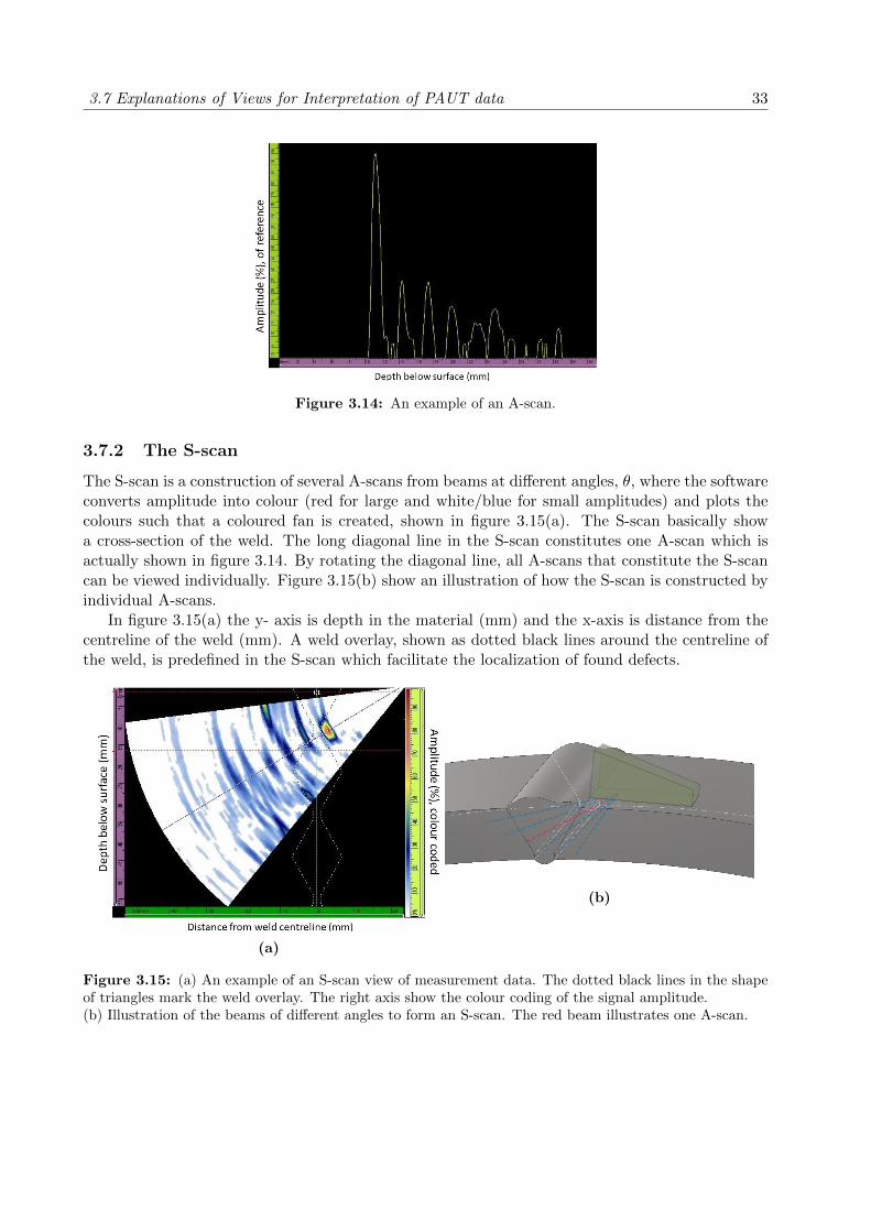
The A-scan, shown in figure 3.14, is the most fundamental view and is a plot of signal amplitude inpercent of a decibel (dB) reference value, versus time. If the PAUT set-up is correctly configuredthe A-scan can plot amplitude (%) versus depth below surface (mm). The A-scan can be used asa tool to determine the type of defect by looking the peak shape and peak size, [48, 53]
3.7 Explanations of Views for Interpretation of PAUT data 33
Figure 3.14: An example of an A-scan.
3.7.2 The S-scan
The S-scan is a construction of several A-scans from beams at different angles, θ, where the softwareconverts amplitude into colour (red for large and white/blue for small amplitudes) and plots thecolours such that a coloured fan is created, shown in figure 3.15(a). The S-scan basically showa cross-section of the weld. The long diagonal line in the S-scan constitutes one A-scan which isactually shown in figure 3.14. By rotating the diagonal line, all A-scans that constitute the S-scancan be viewed individually. Figure 3.15(b) show an illustration of how the S-scan is constructed byindividual A-scans.
In figure 3.15(a) the y- axis is depth in the material (mm) and the x-axis is distance from thecentreline of the weld (mm). A weld overlay, shown as dotted black lines around the centreline ofthe weld, is predefined in the S-scan which facilitate the localization of found defects.
(a)
(b)
Figure 3.15: (a) An example of an S-scan view of measurement data. The dotted black lines in the shapeof triangles mark the weld overlay. The right axis show the colour coding of the signal amplitude.(b) Illustration of the beams of different angles to form an S-scan. The red beam illustrates one A-scan.
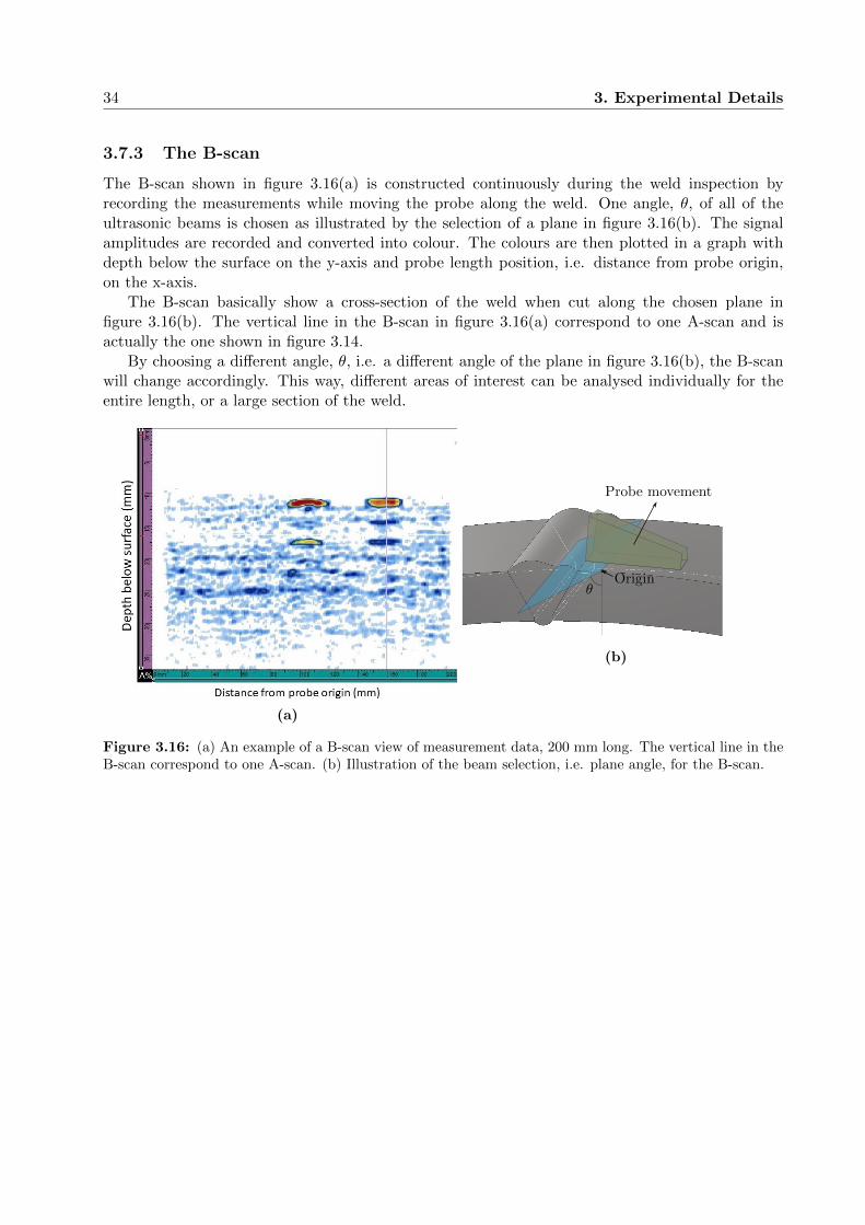
34 3. Experimental Details
3.7.3 The B-scan
The B-scan shown in figure 3.16(a) is constructed continuously during the weld inspection byrecording the measurements while moving the probe along the weld. One angle, θ, of all of theultrasonic beams is chosen as illustrated by the selection of a plane in figure 3.16(b). The signalamplitudes are recorded and converted into colour. The colours are then plotted in a graph withdepth below the surface on the y-axis and probe length position, i.e. distance from probe origin,on the x-axis.
The B-scan basically show a cross-section of the weld when cut along the chosen plane infigure 3.16(b). The vertical line in the B-scan in figure 3.16(a) correspond to one A-scan and isactually the one shown in figure 3.14.
By choosing a different angle, θ, i.e. a different angle of the plane in figure 3.16(b), the B-scanwill change accordingly. This way, different areas of interest can be analysed individually for theentire length, or a large section of the weld.
(a)
θOrigin
Probe movement
(b)
Figure 3.16: (a) An example of a B-scan view of measurement data, 200 mm long. The vertical line in theB-scan correspond to one A-scan. (b) Illustration of the beam selection, i.e. plane angle, for the B-scan.

3.7 Explanations of Views for Interpretation of PAUT data 35
3.7.4 The C-scan
To create the C-scan the software takes all the B-scans and compresses them into one plot andthe result is shown in figure 3.17(a). The x-axis is the distance from origin, and the y-axis is theθ-angle. In other words, each angle (horizontal line) in the C-scan correspond to one B-scan whichis illustrated in figure 3.17(b).
The horizontal line in figure 3.17(b) correspond to the B-scan in figure 3.16(b).To make the C-scan more useful, one can choose to only visualize parts of the information by
placing a gate that selects only the information that was acquired from signals that travelled acertain distance. This was done for the C-scan shown in figure 3.17(a).
(a)
Probe movement
Origin
(b)
Figure 3.17: (a) An example of a C-scan view of measurement data, 200 mm long. (b) Illustration of thebeam selection for the C-scan.


4
ULTRASONIC BEAM DYNAMICS AND COMPARISONOF PAUT FOCAL LAWS
4.1 The Effect of Structure of the Weld Material on UltrasonicBeam Dynamics
Figure 4.1 show a microscopy image of the cross-section of the 11 T dipole horizontal austeniticstainless steel weld. The surface was polished and oxalic etched. The general structure of theweld can be seen and the individual weld passes can be distinguished as dark/white ”interfaces”,especially clear for the first four root passes. A clear difference between weld metal and parentmetal is observed where the weld metal is rather rough and disordered while the parent metal hasan ordered and even structure.
The theory section describes the austenitic stainless steel weld material as very coarse grainedwith columnar grains in the order of millimetres, the same size scale as the weld defects that mustbe detected. The structure that can be seen in the weld material in figure 4.1 matches the descrip-tion of the grain structure in the theory section, but it has not been definitively confirmed that thestructures seen are the individual grains.
The first three weld passes has a rather circular melt area and the columnar structures (possiblythe grains) are oriented towards the centre of the circles, i.e. parallel with the thermal gradient,which was predicted for grain growth during solidification of the weld pool, according to the theory.
The remaining weld passes are rather wide and flat. The width of the weld passes increases foreach new layer, but eventually the width of the gap becomes too big and the weld cannot coverit completely with the melt. Around weld pass number seven, when roughly half of the weld wascompleted, the next pass was placed on one side of the weld region, to the right in figure 4.1. Thiscauses the structures to be tilted towards the top-left corner of the figure, thus the weld is no longersymmetrical around the weld axis.
This anisotropic structure affects the behaviour of the ultrasonic beams that is used for weldquality inspection. Placing the ultrasonic probe on either side of the weld cap result in differentsensitivity to defects in various positions because of the anisotropy. The beam path deviation, beamsplitting and scattering as discussed in the theory section is going to be different when measuringfrom either sides and must be taken into account.
37

38 4. Ultrasonic Beam Dynamics and Comparison of PAUT Focal Laws
(a)
(b)
(c)
(d)
Figure 4.1: Metallographic cross-section of the 11 T dipole weld. The individual weld passes can beidentified and a columnar structure, tilted towards the top-left corner of the image can be seen. More detailsin areas (a), (b), (c) and (d) are given in figure 4.2. Courtesy M. Meyer, CERN, EN-MME.
Figure 4.2(b) show the 316LN parent metal and shows horizontal lines in a structure that isvery different from the weld metal. The backing plate shown in figure 4.2(a) show a homogeneousisotropic structure. The parent metal structures could be explained by the process when formingthe backing plate and the original plates of the half shells [54]. Assuming that the structuresobserved in the images are in fact the grains, then grain coarsening is observed close to the weldfusion line with an almost quadrupling of the grain size. Still, the grain size is significantly smallerthan in the weld metal which is best seen in figure 4.2(c)
Figure 4.2(c) and 4.2(d) show the fusion of weld material to the weld bevel and the centreweld metal respectively. Again, assuming that it is the individual grains that is seen, a sub-grain micro-structure is clearly observed inside the grains, and both columnar and equiaxed sub-grain structure can be identified. (This is also supported in the literature of 316LN austeniticstainless steel weld material [36] presented in the theory section, however must be confirmed by adifferent microscopy method.) Because of the inhomogeneities presented in sub-grain boundariessuch as different chemical composition and lattice disorders, the ultrasonic waves suffer from higherattenuation and scattering compared to a weld material without sub-grain structure.
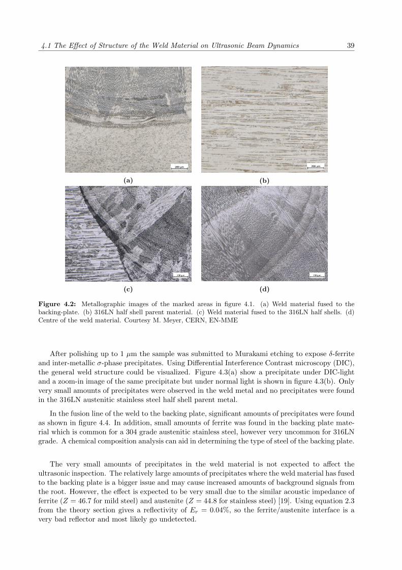
4.1 The Effect of Structure of the Weld Material on Ultrasonic Beam Dynamics 39
(a) (b)
(c) (d)
Figure 4.2: Metallographic images of the marked areas in figure 4.1. (a) Weld material fused to thebacking-plate. (b) 316LN half shell parent material. (c) Weld material fused to the 316LN half shells. (d)Centre of the weld material. Courtesy M. Meyer, CERN, EN-MME
After polishing up to 1 µm the sample was submitted to Murakami etching to expose δ-ferriteand inter-metallic σ-phase precipitates. Using Differential Interference Contrast microscopy (DIC),the general weld structure could be visualized. Figure 4.3(a) show a precipitate under DIC-lightand a zoom-in image of the same precipitate but under normal light is shown in figure 4.3(b). Onlyvery small amounts of precipitates were observed in the weld metal and no precipitates were foundin the 316LN austenitic stainless steel half shell parent metal.
In the fusion line of the weld to the backing plate, significant amounts of precipitates were foundas shown in figure 4.4. In addition, small amounts of ferrite was found in the backing plate mate-rial which is common for a 304 grade austenitic stainless steel, however very uncommon for 316LNgrade. A chemical composition analysis can aid in determining the type of steel of the backing plate.
The very small amounts of precipitates in the weld material is not expected to affect theultrasonic inspection. The relatively large amounts of precipitates where the weld material has fusedto the backing plate is a bigger issue and may cause increased amounts of background signals fromthe root. However, the effect is expected to be very small due to the similar acoustic impedance offerrite (Z = 46.7 for mild steel) and austenite (Z = 44.8 for stainless steel) [19]. Using equation 2.3from the theory section gives a reflectivity of Er = 0.04%, so the ferrite/austenite interface is avery bad reflector and most likely go undetected.
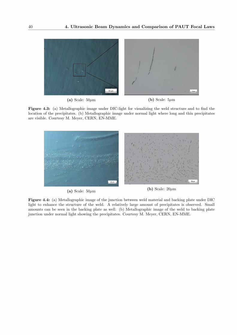
40 4. Ultrasonic Beam Dynamics and Comparison of PAUT Focal Laws
(a) Scale: 50µm (b) Scale: 5µm
Figure 4.3: (a) Metallographic image under DIC-light for visualizing the weld structure and to find thelocation of the precipitates. (b) Metallographic image under normal light where long and thin precipitatesare visible. Courtesy M. Meyer, CERN, EN-MME.
(a) Scale: 50µm(b) Scale: 20µm
Figure 4.4: (a) Metallographic image of the junction between weld material and backing plate under DIClight to enhance the structure of the weld. A relatively large amount of precipitates is observed. Smallamounts can be seen in the backing plate as well. (b) Metallographic image of the weld to backing platejunction under normal light showing the precipitates. Courtesy M. Meyer, CERN, EN-MME.

4.2 The Effect of the Stainless Steel Half Shells on Ultrasonic Beam Dynamics 41
4.2 The Effect of the Stainless Steel Half Shells on UltrasonicBeam Dynamics
4.2.1 Wedge-Surface Distance
For a good coupling of sound from the wedge and the test object, the gap between the wedge andtest piece should not exceed d = 0.50 mm according to ISO 17640 [13]. Because the wedge shoe isflat and the cylindrical 11 T dipole magnet surface is not, only a small part of the wedge in actualcontact with the magnet surface and a gap is obtained, illustrated in figure 4.5. Water is used as acoupling medium between the wedge and the surface. The water is continuously pumped throughthe irrigation ports of the wedge which ensures that a film of water is obtained between the twosurfaces throughout the scan.
y
x
R
(x1, y1) (x2, y2)
r =√x2 + y2
d(x0, y0)
Figure 4.5: An exaggerated illustration of the gap between wedge and surface due to curvature.
Assuming that the contact point (x0, y0) = (0.0, 0.0) of the wedge coincides with the beam exitpoint, i.e. the point where maximum wave energy leaves the wedge, one can calculate the wedgeto surface distance for any point of the wedge using the equation 4.1.
d = r −R =√x2 + y2 −R (4.1)
The maximum width of the beam was calculated where point 1 and point 2 in figure 4.5 is theextreme ends where the beam exits the wedge. Point 1 was calculated to (x1, y1) = (−9.1, 285.0)mm, which gives d = 0.15 mm. Point 2 was calculated to (x2, y2) = (8.5, 285.0) mm, which givesd = 0.13 mm. The requirement that d<0.50 mm is fulfilled with good margin, and therefore thewedge can be used without any changes to its dimensions.
4.2.2 Beam Spread due to the Cylindrical Surface
The use of a flat wedge in the inspection of the cylindrical 11 T dipole horizontal welds will causea significant beam spread which must be taken into account for the interpretation of the PAUTresults, especially when determining the position of potential weld defects. Snells law states thatthe refraction and reflection angles depend on the incidence angle of the ultrasonic beam accordingto equation 2.5, as described in theory.
Figure 4.6 illustrate the refraction angles obtained for a beam without beam steering or focusing.The blue area shows the beam refraction if a flat surface was inspected. The green area shows theadditional coverage when inspecting on the cylindrical surface of the 11 T dipole magnets.

42 4. Ultrasonic Beam Dynamics and Comparison of PAUT Focal Laws
Figure 4.7 show a graph of the beam spread that is obtained in the inspection of the 11 Tdipole half shell welds if no focusing of the ultrasonic beam is used. Point A, AB, B, BC and C isindicated in figure 4.6.
Most of the ultrasonic energy exits the wedge close to point B, which has about the samerefraction angle as when inspecting an object with a flat surface. This means that defects aredetected with the strongest signal amplitude at, or very close to, the correct angle.
The graph shows that the beam spread between point AB and BC is much less than betweenpoint A and C. When considering this centre part of the ultrasonic beam, the total beam spread isabout +3◦ and -2.5◦ for a 55◦ beam. For beam steering above 72.5◦, the total beam spread reachesits maximum, and parts of the ultrasonic beam is propagating at a 90◦ angle, i.e. parallel to thesurface.
Beam spread has a negative impact on sizing of defects where they appear larger than normaland the noise level will increase due to dispersed energy from the desired area to the surroundings.For beam steering above 72.5◦ a large portion of the beam is expected to travel close to the surfacewhich can be used for detection of surface and near surface defects, although with a weak signalamplitude. The depth localization and sizing of near surface defects in the PAUT set-up are notaccurate where defects appear smaller than they actually are, and at a deeper position in the weldvolume.
AB
C ABBC
Figure 4.6: Ultrasonic beam spread due to the inspection of a curved surface. The blue area shows beampropagation in the case of a flat piece (dotted lines). The blue and green area combined is for curved surface(dashed lines).

4.2 The Effect of the Stainless Steel Half Shells on Ultrasonic Beam Dynamics 43
Figure 4.7: Graph showing the calculated beam spread of the refraction angles obtained in the 11 T dipolehalf shells versus incidence angles in the wedge. Beams above approximately 70◦ have a particularly largebeam spread. The curves are calculated for the beams originating from point A, AB, B, BC, and C infigure 4.6. The solid line indicates the refraction angle for an inspection on a flat surface.
4.2.3 Beam Angle Offset due to the Cylindrical Surface
The curvature of the surface of the 11 T dipole magnet, and the wedge displacement from thecentre of the tube creates an angle offset, α, shown in figure 4.8. This offset angle was calculatedfor the case that the probe is placed 2 mm apart from the weld cap (a + b = 22 mm from weldcentre) which gives α = 4.4◦. For example, the 53◦ beam is offset by 4.4◦ to β = 53 + α = 57.4◦.
This affects the accuracy of determining the position of the defects. Defects appear to resideshallower than their actual position.
a b
α
53◦
β
Figure 4.8: Illustration of the angle offset, α, due to the curvature of the 11 T dipole half shell.

44 4. Ultrasonic Beam Dynamics and Comparison of PAUT Focal Laws
4.3 Comparison of PAUT Focal Laws
In order to compare different focal laws, and to determine a good focal law for the PAUT inspectionof the 15 mm thick austenitic stainless steel welds of the 11 T dipole magnets, a flat 16 mm thick,austenitic stainless steel block was used, shown in figure 4.9.
∅ = 2 mm SDHs and 1.5 mm deep notches were machined in various positions in the block.Five areas have been marked with a permanent pen, and each area simulate a weld with defects.The probe was placed parallel to and close to the ”weld” area which would be the case duringa real weld inspection. Only the signals from identical artificial defects at different positions wascompared, therefore the SDHs in ”weld” areas 1, 2 and 5 were used.
Four different focal laws with focus at 15 mm, 20 mm, 25 mm and 30 mm sound path have beencompared for sensitivity and for their accuracy of locating the artificial defects in depth below thesurface, length away from the probe and the length of the sound path. No sensitivity calibrationwas done for these measurements since it would interfere with the focusing effects of the calculatedfocal laws. However, range calibration was necessary to get representative distance readings.
The two focal laws with focus at 25 mm and 30 mm sound path were found to have the bestaccuracy in determining the position of the defects. The different focal laws sensitivity to detectthe SDHs was also compared. After considering the defocusing properties, i.e. beam spread, of thecylindrical surface of the half shells, a focus of 20 mm or 25 mm sound path was found to have thestrongest sensitivity to the defects.
From these comparisons, a focal law with focus at 25 mm sound path was determined to havethe best properties for the inspection of the 11 T dipole horizontal welds.
1. 2. 3.
4. 5(a) 5(b)
Figure 4.9: A 16 mm thick flat austenitic stainless steel block with SDHs and notches. The black penmarkings show a ”weld” area(1, 2, 3, 4 and 5) with artificial defects.
4.3.1 The Effect of the Range of Beam Steering Angles
Ultrasonic inspections that uses longitudinal wave probes suffer from mode converted signals, i.e.a conversion from longitudinal waves into shear waves as described in the theory section. Thiseffect is mostly observed for angled ultrasonic beam inspections. The amount of mode conversionincreases with the incidence angle of the ultrasonic beam [20]. An angled beam inspection is used

4.3 Comparison of PAUT Focal Laws 45
for the 11 T dipole half shell welds, where the phased array probe is producing longitudinal waves,incident with an angle towards the half shell surface.
To avoid an excessive amount of mode converted signals which can cause confusion in theinterpretation of the data, a maximum beam steering angle of 80◦ was chosen. Similarly, to avoidexcessive number of signals from the beams that are reflected from the backside of the half shells,a minimum beam steering angle of 40◦ was chosen.
4.3.2 The Effect of Focus Length on Distance Readings
To compare the differences in distance readings due to the focus length of the focal law, the probewas placed facing each of the ”weld” areas, and readings from all four focal laws were taken withoutmoving the probe. The depth, length and sound path distances were measured with a ruler andis shown in table 4.1. Based on these measurements, the required ultrasonic beam angle wascalculated.
Table 4.1: Measured distances using a ruler for the reflectors of each ”weld” area of the block in figure 4.9.The left side of area 5 is called 5(a) the right side is called 5(b).
Reflector Angle (◦) Depth(mm)
Length(mm)
Sound Path(mm)
1. SDH 67.8 8.5 10.5 22.52. Bottom SDH 60 12 10 242. Top SDH 81.8 3 10 215(a) Top SDH 84.3 3 18.5 305(a) Bottom SDH 66.9 11 14 285(b) Top SDH 76.1 3 1 12.55(b) Bottom SDH 56.6 11 5.5 20
The distance readings from the PAUT inspection are given in table 4.2 for each of the focuslengths. The difference between the measured distance and the actual distance is presented initalic.
On average, the depth measurements for the four focal laws are a bit too shallow and the lengthmeasurements a bit too long. The sound path measurement is very accurate and deviate less than1 mm for most echoes. The exception is when focus is placed very close to the probe at 15 mmsound path, and for the reflections at very large angles, above 75◦.
The focal laws with focus at 25 mm and 30 mm has length, depth and sound path measurementswhich deviate less than 1 mm for most SDHs. The focal law with focus at 30 mm sound path showthe most accurate distance measurements. The two other focal laws with focus at 15 mm and 20mm sound path have deviations in length, depth and sound path larger than 1 mm for many SDHs.It was therefore decided that these two focal laws will not be used for weld inspection.
The special cases when the required ultrasonic beam angle is larger than 80◦ to reach the SDHsare interesting because these defects are still detectable although beam steering is limited between40◦ to 80◦. However, the amplitude of the signals from these defects are very low.
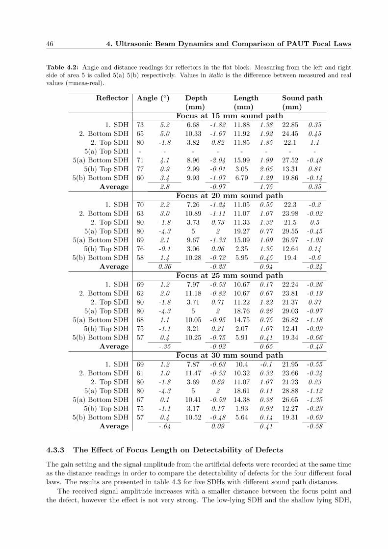
46 4. Ultrasonic Beam Dynamics and Comparison of PAUT Focal Laws
Table 4.2: Angle and distance readings for reflectors in the flat block. Measuring from the left and rightside of area 5 is called 5(a) 5(b) respectively. Values in italic is the difference between measured and realvalues (=meas-real).
Reflector Angle (◦) Depth(mm)
Length(mm)
Sound path(mm)
Focus at 15 mm sound path1. SDH 73 5.2 6.68 -1.82 11.88 1.38 22.85 0.35
2. Bottom SDH 65 5.0 10.33 -1.67 11.92 1.92 24.45 0.452. Top SDH 80 -1.8 3.82 0.82 11.85 1.85 22.1 1.1
5(a) Top SDH - - - - - - - -5(a) Bottom SDH 71 4.1 8.96 -2.04 15.99 1.99 27.52 -0.48
5(b) Top SDH 77 0.9 2.99 -0.01 3.05 2.05 13.31 0.815(b) Bottom SDH 60 3.4 9.93 -1.07 6.79 1.29 19.86 -0.14
Average 2.8 -0.97 1.75 0.35
Focus at 20 mm sound path1. SDH 70 2.2 7.26 -1.24 11.05 0.55 22.3 -0.2
2. Bottom SDH 63 3.0 10.89 -1.11 11.07 1.07 23.98 -0.022. Top SDH 80 -1.8 3.73 0.73 11.33 1.33 21.5 0.5
5(a) Top SDH 80 -4.3 5 2 19.27 0.77 29.55 -0.455(a) Bottom SDH 69 2.1 9.67 -1.33 15.09 1.09 26.97 -1.03
5(b) Top SDH 76 -0.1 3.06 0.06 2.35 1.35 12.64 0.145(b) Bottom SDH 58 1.4 10.28 -0.72 5.95 0.45 19.4 -0.6
Average 0.36 -0.23 0.94 -0.24
Focus at 25 mm sound path1. SDH 69 1.2 7.97 -0.53 10.67 0.17 22.24 -0.26
2. Bottom SDH 62 2.0 11.18 -0.82 10.67 0.67 23.81 -0.192. Top SDH 80 -1.8 3.71 0.71 11.22 1.22 21.37 0.37
5(a) Top SDH 80 -4.3 5 2 18.76 0.26 29.03 -0.975(a) Bottom SDH 68 1.1 10.05 -0.95 14.75 0.75 26.82 -1.18
5(b) Top SDH 75 -1.1 3.21 0.21 2.07 1.07 12.41 -0.095(b) Bottom SDH 57 0.4 10.25 -0.75 5.91 0.41 19.34 -0.66
Average -.35 -0.02 0.65 -0.43
Focus at 30 mm sound path1. SDH 69 1.2 7.87 -0.63 10.4 -0.1 21.95 -0.55
2. Bottom SDH 61 1.0 11.47 -0.53 10.32 0.32 23.66 -0.342. Top SDH 80 -1.8 3.69 0.69 11.07 1.07 21.23 0.23
5(a) Top SDH 80 -4.3 5 2 18.61 0.11 28.88 -1.125(a) Bottom SDH 67 0.1 10.41 -0.59 14.38 0.38 26.65 -1.35
5(b) Top SDH 75 -1.1 3.17 0.17 1.93 0.93 12.27 -0.235(b) Bottom SDH 57 0.4 10.52 -0.48 5.64 0.14 19.31 -0.69
Average -.64 0.09 0.41 -0.58
4.3.3 The Effect of Focus Length on Detectability of Defects
The gain setting and the signal amplitude from the artificial defects were recorded at the same timeas the distance readings in order to compare the detectability of defects for the four different focallaws. The results are presented in table 4.3 for five SDHs with different sound path distances.
The received signal amplitude increases with a smaller distance between the focus point andthe defect, however the effect is not very strong. The low-lying SDH and the shallow lying SDH,

4.3 Comparison of PAUT Focal Laws 47
”5(b) Bottom SDH” and ”5(a) Top SDH” respectively, had the same gain setting for the focal laws,and clearly show that using a focus distance which is close to the defect gives a stronger signal.
The sensitivity of the inspection is dependent on the angle of the ultrasonic beam where largerangles require more gain to raise the signal amplitude of the defects to approximately 80% whichis also shown in table 4.3. This is the reason why the angular-corrected-gain (ACG) sensitivitycalibration is required. The shallow defects which theoretically require an ultrasonic beam above80◦ is detected in this PAUT set-up, however the gain required to raise their signal amplitudes arevery large.
The sound path distances to the areas of interest are approximately between 20 and 30 mm.Therefore, after considering the defocusing properties (beam spread) of the cylindrical geometry inthe inspection of the 11 T dipole magnets, a focus between 20 and 25 mm should be considered.
Table 4.3: Comparison of amplitude response of five defects shown in figure 4.9 for the four focal laws.The gain and amplitude is presented along with distance between focal point and defect for each focal law.
Focuslength(mm)
Distance, focusto defect (mm)
Gain (dB) Amplitude (%)
1. SDH, 22.5 mm sound path(67.8◦)
15 -7.5 34 8020 -2.5 31 7425 2.5 31 7330 7.5 31 70
2. Bottom SDH, 24 mm sound path (60◦)
15 -9 34 8520 -4 31 8225 1 31 8730 6 31 83
5(b) Bottom SDH, 20 mm sound path (56.6◦)
15 -5 27 7020 0 27 8625 5 27 8330 10 27 77
5(b) Top SDH, 12,5 mm sound path (76.1◦)
15 2.5 33 8320 7.5 33 7225 12.5 33 5730 17.5 33 51
5(a) Top SDH, 30 mm sound path (84.3◦)
15 -15 - -20 -10 48 5225 -5 46 5430 0 46 58

48 4. Ultrasonic Beam Dynamics and Comparison of PAUT Focal Laws
4.4 Discussion of the Results of Ultrasonic Beam Dynamics andComparison of PAUT Focal Laws
The microscopy of the 11 T dipole weld cross-section revealed an asymmetric weld structure wherethe sonic properties, according to the theory (chapter 2), is different when inspecting from eitherside of the weld.
The geometry of the horizontal welds of the 11 T half shells affects the ultrasonic beam dynamicsand must be taken into account in the interpretation of the results. Weld imperfections will appearlarger than normal due to the beam spread caused by the cylindrical surface. In addition, shallowdefects, reached by ultrasonic beams larger than 70◦-75◦ will appear as surface breaking defectsindependently if they are or not (figure 4.7).
Furthermore, the cylindrical geometry of the half shell welds causes an offset of +4.4◦ of theultrasonic beam as shown in figure 4.8, causing defects to appear more shallow than the actualcase. However, unlike the calculations, the real half shell weld area is not a perfect cylinder anddissimilarities in the geometry is difficult to predict, so the offset can differ slightly. Though theeffect is quite small as shown in chapter 5.
Several different PAUT focal laws have been calculated. Through the comparison of distancereadings and signal amplitude for different focus lengths, a focal law with focus at 25 mm soundpath has been selected for the routine inspection of the 15 mm thick austenitic stainless steel 11 Tdipole welds. The defocusing properties (beam spread) due to the cylindrical geometry of the halfshells and the sound path distance to the area of interest were taken into account.
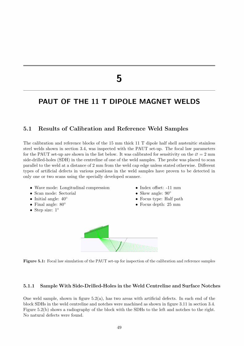
5
PAUT OF THE 11 T DIPOLE MAGNET WELDS
5.1 Results of Calibration and Reference Weld Samples
The calibration and reference blocks of the 15 mm thick 11 T dipole half shell austenitic stainlesssteel welds shown in section 3.4, was inspected with the PAUT set-up. The focal law parametersfor the PAUT set-up are shown in the list below. It was calibrated for sensitivity on the ∅ = 2 mmside-drilled-holes (SDH) in the centreline of one of the weld samples. The probe was placed to scanparallel to the weld at a distance of 2 mm from the weld cap edge unless stated otherwise. Differenttypes of artificial defects in various positions in the weld samples have proven to be detected inonly one or two scans using the specially developed scanner.
• Wave mode: Longitudinal compression • Index offset: -11 mm• Scan mode: Sectorial • Skew angle: 90◦
• Initial angle: 40◦ • Focus type: Half path• Final angle: 80◦ • Focus depth: 25 mm• Step size: 1◦
Figure 5.1: Focal law simulation of the PAUT set-up for inspection of the calibration and reference samples
5.1.1 Sample With Side-Drilled-Holes in the Weld Centreline and Surface Notches
One weld sample, shown in figure 5.2(a), has two areas with artificial defects. In each end of theblock SDHs in the weld centreline and notches were machined as shown in figure 3.11 in section 3.4.Figure 5.2(b) shows a radiography of the block with the SDHs to the left and notches to the right.No natural defects were found.
49

50 5. PAUT of the 11 T Dipole Magnet Welds
(a)
SDHs Notches
(b)
Figure 5.2: (a) Image of the centreline SDH weld sample where two SDHs can be seen in the front of theblock and two top surface notches can be seen in back. (b) Top view radiographic image of the centrelineSDH weld sample where the SDHs are seen as one dark line because they overlap. The bottom and top centrenotches overlap slightly while the side notches are clearly distinguished. No natural defects were found.
The weld sample was inspected from both sides of the weld with the probes parallel to the weldat a 2 mm distance from the weld cap. Two significantly different responses from the centrelineSDHs were received. For the left-side inspection (figure 5.3(a)) the amplitudes were 140% and151% FSH for respective hole. In the right-side inspection (figure 5.3(b)), the amplitudes were85% and 81% FSH for the top and bottom SDH respectively. The sensitivity ACG calibration ofthe PAUT-setup was performed on these SDHs from the right side (figure 5.3(b)) which thereforeshould show 80% full-screen-height (FSH). However, the probe position was not exactly the samefor the inspection as for calibration so small differences were observed.
In the inspection from the left side, the probe could be placed closer to the SDHs due to theconstraints of the weld cap, and therefore a shorter sound path to the hole of approximately 2 mmwas obtained. This and the anisotropy of the weld material, where ultrasonic beams of differentdirections are not equally attenuated as discussed in the theory chapter, could explain why theamplitude response is so much larger for this side. As expected, these defects would be judgedunacceptable according to sensitivity level 2 from ISO 11666, particularly when viewed from theleft side of the weld.
(a) (b)
Figure 5.3: Left (a) and right (b) side S-scan respectively for the SDH area. The direct signals are markedwith arrows. The other signals are combinations of skipped and mode-converted beams.

5.1 Results of Calibration and Reference Weld Samples 51
The detection of the 1 mm deep notches (counted from the half shell surface) are a bit moredifficult to distinguish. The notch in the weld bevel is clearly detected with the direct reflection,shown in figure 5.4(a). The root notch has only a very weak direct signal and the centreline notchdoes not have one at all. Therefore it is necessary to look for the secondary signals in the skippedbeam and mode converted zone, shown in figure 5.4(b).
The mode converted root signal at 75◦ increase in signal amplitude significantly to 88% FSHfrom background (30%-50%) when inspecting the root notch. The 55 mm long root notch signalcan be distinguished from the 45 mm long centreline notch signals since these appear shorter in thescan by approximately 12 mm, consistent with the actual length of the notches. Two secondarysignals from the 45 mm long notch have large amplitudes of 78% and 104%. A short signal of 65%amplitude, approximately 7 mm long, appear at the position of a 10 mm long shallow notch in thesurface of the block.
Although it is possible to detect the notches through the mode converted and skipped secondarysignals, it is required to have a direct signal to determine whether they are conforming or not. Thiscan be obtained if the weld cap is removed.
The root notch did not cause a strong direct signal because it was not machined in the correctposition due to a design error. A root notch is typically a very strong reflector, however in thissample it was machined inside the junction between the weld and the backing plate. The normalcase is to machine the root notch on the side of this junction.
(a)
(b)
Figure 5.4: (a) S-scan from the left side of the weld with notches. Arrows marks the direct signals from thesurface notch in the weld fusion line and the root notch. (b) A 60 mm long 75◦ B-scan showing the skipped/mode converted signals of the notches. The black arrows mark the signals from the surface centreline notch,the yellow arrow mark the longer root notch signal and the red arrow mark the signal from a small surfacenotch.
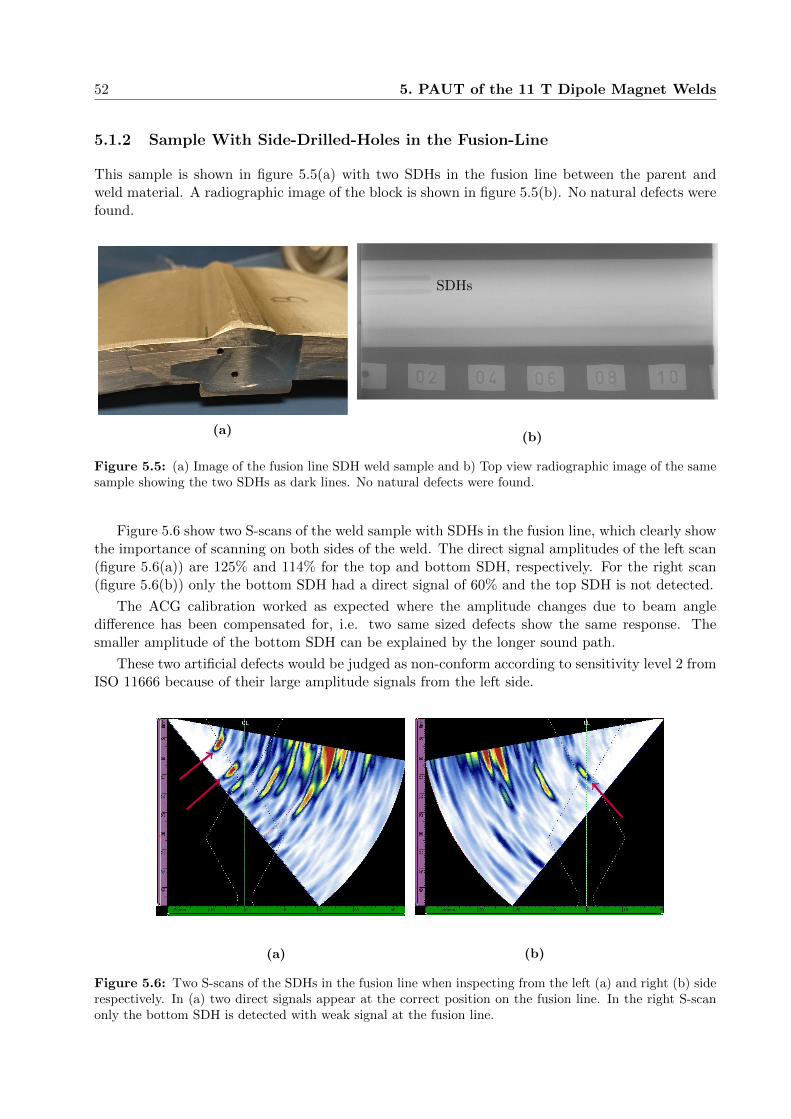
52 5. PAUT of the 11 T Dipole Magnet Welds
5.1.2 Sample With Side-Drilled-Holes in the Fusion-Line
This sample is shown in figure 5.5(a) with two SDHs in the fusion line between the parent andweld material. A radiographic image of the block is shown in figure 5.5(b). No natural defects werefound.
(a)
SDHs
(b)
Figure 5.5: (a) Image of the fusion line SDH weld sample and b) Top view radiographic image of the samesample showing the two SDHs as dark lines. No natural defects were found.
Figure 5.6 show two S-scans of the weld sample with SDHs in the fusion line, which clearly showthe importance of scanning on both sides of the weld. The direct signal amplitudes of the left scan(figure 5.6(a)) are 125% and 114% for the top and bottom SDH, respectively. For the right scan(figure 5.6(b)) only the bottom SDH had a direct signal of 60% and the top SDH is not detected.
The ACG calibration worked as expected where the amplitude changes due to beam angledifference has been compensated for, i.e. two same sized defects show the same response. Thesmaller amplitude of the bottom SDH can be explained by the longer sound path.
These two artificial defects would be judged as non-conform according to sensitivity level 2 fromISO 11666 because of their large amplitude signals from the left side.
(a) (b)
Figure 5.6: Two S-scans of the SDHs in the fusion line when inspecting from the left (a) and right (b) siderespectively. In (a) two direct signals appear at the correct position on the fusion line. In the right S-scanonly the bottom SDH is detected with weak signal at the fusion line.
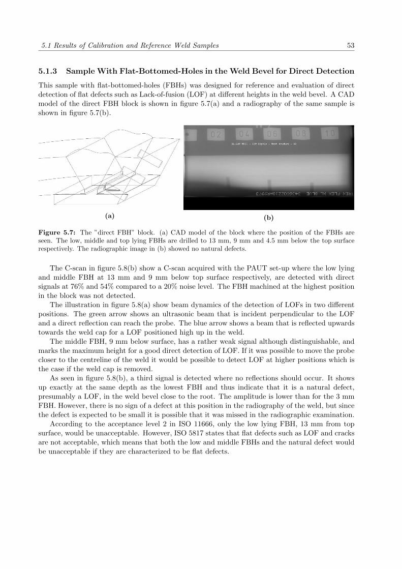
5.1 Results of Calibration and Reference Weld Samples 53
5.1.3 Sample With Flat-Bottomed-Holes in the Weld Bevel for Direct Detection
This sample with flat-bottomed-holes (FBHs) was designed for reference and evaluation of directdetection of flat defects such as Lack-of-fusion (LOF) at different heights in the weld bevel. A CADmodel of the direct FBH block is shown in figure 5.7(a) and a radiography of the same sample isshown in figure 5.7(b).
(a) (b)
Figure 5.7: The ”direct FBH” block. (a) CAD model of the block where the position of the FBHs areseen. The low, middle and top lying FBHs are drilled to 13 mm, 9 mm and 4.5 mm below the top surfacerespectively. The radiographic image in (b) showed no natural defects.
The C-scan in figure 5.8(b) show a C-scan acquired with the PAUT set-up where the low lyingand middle FBH at 13 mm and 9 mm below top surface respectively, are detected with directsignals at 76% and 54% compared to a 20% noise level. The FBH machined at the highest positionin the block was not detected.
The illustration in figure 5.8(a) show beam dynamics of the detection of LOFs in two differentpositions. The green arrow shows an ultrasonic beam that is incident perpendicular to the LOFand a direct reflection can reach the probe. The blue arrow shows a beam that is reflected upwardstowards the weld cap for a LOF positioned high up in the weld.
The middle FBH, 9 mm below surface, has a rather weak signal although distinguishable, andmarks the maximum height for a good direct detection of LOF. If it was possible to move the probecloser to the centreline of the weld it would be possible to detect LOF at higher positions which isthe case if the weld cap is removed.
As seen in figure 5.8(b), a third signal is detected where no reflections should occur. It showsup exactly at the same depth as the lowest FBH and thus indicate that it is a natural defect,presumably a LOF, in the weld bevel close to the root. The amplitude is lower than for the 3 mmFBH. However, there is no sign of a defect at this position in the radiography of the weld, but sincethe defect is expected to be small it is possible that it was missed in the radiographic examination.
According to the acceptance level 2 in ISO 11666, only the low lying FBH, 13 mm from topsurface, would be unacceptable. However, ISO 5817 states that flat defects such as LOF and cracksare not acceptable, which means that both the low and middle FBHs and the natural defect wouldbe unacceptable if they are characterized to be flat defects.
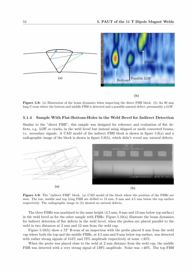
54 5. PAUT of the 11 T Dipole Magnet Welds
(a)Bottom
Possible LOF
Middle
(b)
Figure 5.8: (a) Illustration of the beam dynamics when inspecting the direct FBH block. (b) An 80 mmlong C-scan where the bottom and middle FBH is detected and a possible natural defect, presumably a LOF.
5.1.4 Sample With Flat-Bottom-Holes in the Weld Bevel for Indirect Detection
Similar to the ”direct FBH”, this sample was designed for reference and evaluation of flat de-fects, e.g. LOF or cracks, in the weld bevel but instead using skipped or mode converted beams,i.e. secondary signals. A CAD model of the indirect FBH block is shown in figure 5.9(a) and aradiographic image of the block is shown in figure 5.9(b), which didn’t reveal any natural defects.
(a)(b)
Figure 5.9: The ”indirect FBH” block. (a) CAD model of the block where the position of the FBHs areseen. The low, middle and top lying FBH are drilled to 13 mm, 9 mm and 4.5 mm below the top surfacerespectively. The radiographic image in (b) showed no natural defects.
The three FBHs was machined to the same height (4.5 mm, 9 mm and 13 mm below top surface)in the weld bevel as for the other sample with FBHs. Figure 5.10(a) illustrate the beam dynamicsfor indirect detection of flat defects in the weld bevel, when the probes are placed parallel to theweld in two distances at 2 mm and 12 mm from the weld cap.
Figure 5.10(b) show a 72◦ B-scan of an inspection with the probe placed 6 mm from the weldcap where both the top and the middle FBHs, at 4.5 mm and 9 mm below top surface, was detectedwith rather strong signals of 154% and 72% amplitude respectively at noise <35%.
When the probe was placed close to the weld at 2 mm distance from the weld cap, the middleFBH was detected with a very strong signal of 139% amplitude. Noise was <40%. The top FBH

5.1 Results of Calibration and Reference Weld Samples 55
was barely detected in this probe configuration. Moving the probe further away from the weld to12 mm from the weld cap, a large signal for the top lying FBH at 201% was obtained, comparedto noise level <40%. The FBH machined 13 mm below surface, was not detected in any probeconfiguration.
The acceptability of these artificial defects cannot be concluded from the acceptance levelsin ISO 11666 because they were only identified with secondary signals and not direct detection.Therefore, the weld cap must be removed so the probe can be placed directly on top of the weldand a direct signal can be obtained.
(a)
Top Middle
(b)
Figure 5.10: (a) Illustration of the beam when inspecting the indirect FBH block. The green arrow showprobe position at 2 mm from weld cap and the blue arrow for probe position at 12 mm from weld cap. (b)A 100 mm long B-scan at 72◦ for a probe position at 6 mm from weld cap where both top and middle FBHsare detected.
5.1.5 Sample with Natural Defect
A natural defect was found in the radiography of a 35 cm long block of the same weld material asthe reference and calibration blocks, i.e. the 15 mm thick austenitic stainless steel welds of an 11T dipole prototype magnet. The defect was identified as a shrinkage cavity approximately 7 mmlong and 3 mm wide, shown in figure 5.11(a)
The defect was clearly detected from probes on either side of the weld including when scanningthe heat-affected-zone which indicate that the defect is volumetric and not flat as shown in fig-ure 5.11(b). The signal amplitude was 153% and noise level <25%, which according to ISO 11666is unacceptable.

56 5. PAUT of the 11 T Dipole Magnet Welds
(a)
(b)
Figure 5.11: (a) Radiography and (b) PAUT C-scan of a block with a natural shrinkage groove, approxi-mately 7 mm long and 3 mm wide.
5.1.6 Two Weld Samples from 10 mm Thick LHC Main Dipole Half Shells
Two cylindrical austenitic stainless steel weld samples from an LHC main dipole magnet, 10 mmthick, were tested using the PAUT set-up. They were welded using MIG without backing plate.
A 20 cm long sample weld was inspected with radiography at high energy before artificial defectswere machined into it, which revealed a 1 mm diameter porosity and a 0.5 mm diameter inclusionlocated close to the weld bevel, shown in figure 5.12(a). Three artificial defects were machined andare indicated in the radiography image. One 25 mm long, 2 mm deep saw kerf and a 20 mm long,1 mm deep notch were machined right next to the root. A 30 mm long, ∅ = 2 mm SDH weremachined in the centre of the weld. Two C-scans are shown in figure 5.12(b) and figure 5.12(c) forscanning on the ”close” and ”far” side respectively. The probe position where the ultrasonic beamcan reach the root defects without propagating through the weld material is called ”close-side”, theother is called the ”far-side”.
All three artificial defects were detected with strong signals for both scans, however with slightlydifferent result and with noise level <30%. The saw kerf had a signal amplitude of 140%, and thenotch had 77% signal amplitude for both sides. The signal strength for the SDH differed significantlywhere the ”close” side had 87% and ”far” side had 148%.
The sonic anisotropy of the weld material is observed in the changes of the amplitude for the sawkerf which appear as three distinct points when the beam must travel through the weld materialin the ”far-side” scan. Also, the SDH has significantly different signal amplitude when measuringfrom either side of the weld even though the sound path is the same.
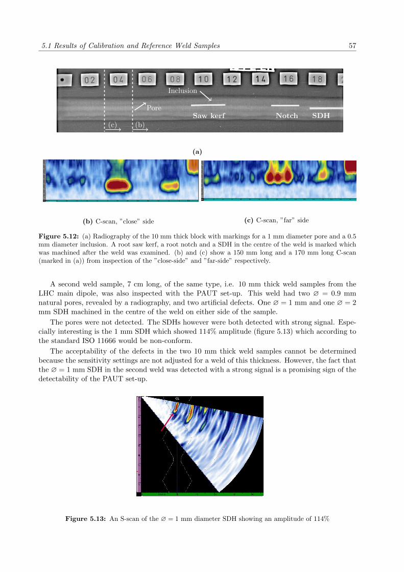
5.1 Results of Calibration and Reference Weld Samples 57
(b)(c)
Pore
Inclusion
Saw kerf Notch SDH
(a)
(b) C-scan, ”close” side (c) C-scan, ”far” side
Figure 5.12: (a) Radiography of the 10 mm thick block with markings for a 1 mm diameter pore and a 0.5mm diameter inclusion. A root saw kerf, a root notch and a SDH in the centre of the weld is marked whichwas machined after the weld was examined. (b) and (c) show a 150 mm long and a 170 mm long C-scan(marked in (a)) from inspection of the ”close-side” and ”far-side” respectively.
A second weld sample, 7 cm long, of the same type, i.e. 10 mm thick weld samples from theLHC main dipole, was also inspected with the PAUT set-up. This weld had two ∅ = 0.9 mmnatural pores, revealed by a radiography, and two artificial defects. One ∅ = 1 mm and one ∅ = 2mm SDH machined in the centre of the weld on either side of the sample.
The pores were not detected. The SDHs however were both detected with strong signal. Espe-cially interesting is the 1 mm SDH which showed 114% amplitude (figure 5.13) which according tothe standard ISO 11666 would be non-conform.
The acceptability of the defects in the two 10 mm thick weld samples cannot be determinedbecause the sensitivity settings are not adjusted for a weld of this thickness. However, the fact thatthe ∅ = 1 mm SDH in the second weld was detected with a strong signal is a promising sign of thedetectability of the PAUT set-up.
Figure 5.13: An S-scan of the ∅ = 1 mm diameter SDH showing an amplitude of 114%

58 5. PAUT of the 11 T Dipole Magnet Welds
5.1.7 Background Signals and Noise of the 11 T Dipole Welds
Figure 5.14 show typical background signals and noise from the 11 T dipole half shell weld inspectionusing the PAUT set-up with probes parallel to the weld and at 2 mm distance from the weld cap.The strong attenuation and scattering of the weld material is seen as increased noise as the ultrasonicbeam enters the weld. Background signal(s) from the root are obtained as weak echoes originatingfrom the fusion interface between the backing plate and the half shells.
The ultrasonic beams above approximately 75◦ have a large percentage of mode conversion intoshear waves which will propagate with a different refraction angle and with approximately halfof the speed of longitudinal waves. This, in combination with a large gain for the high anglesobtained from the sensitivity calibration, gives rather strong background signals of approximately50%. They originate from the different weld features, e.g. the shape of the weld cap or the weld tobacking plate fusion. The inspections on either side of the weld do not show the same backgroundsignals or noise.
The PAUT signals from actual defects can be distinguished from the background since thebackground is always present and does not change much throughout the length of the inspection.
Figure 5.14: Typical background signals and noise for the PAUT set-up when inspecting the 11 T dipolewelds.
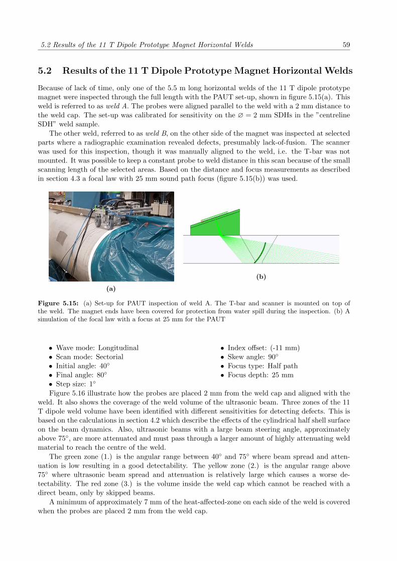
5.2 Results of the 11 T Dipole Prototype Magnet Horizontal Welds 59
5.2 Results of the 11 T Dipole Prototype Magnet Horizontal Welds
Because of lack of time, only one of the 5.5 m long horizontal welds of the 11 T dipole prototypemagnet were inspected through the full length with the PAUT set-up, shown in figure 5.15(a). Thisweld is referred to as weld A. The probes were aligned parallel to the weld with a 2 mm distance tothe weld cap. The set-up was calibrated for sensitivity on the ∅ = 2 mm SDHs in the ”centrelineSDH” weld sample.
The other weld, referred to as weld B, on the other side of the magnet was inspected at selectedparts where a radiographic examination revealed defects, presumably lack-of-fusion. The scannerwas used for this inspection, though it was manually aligned to the weld, i.e. the T-bar was notmounted. It was possible to keep a constant probe to weld distance in this scan because of the smallscanning length of the selected areas. Based on the distance and focus measurements as describedin section 4.3 a focal law with 25 mm sound path focus (figure 5.15(b)) was used.
(a)
(b)
Figure 5.15: (a) Set-up for PAUT inspection of weld A. The T-bar and scanner is mounted on top ofthe weld. The magnet ends have been covered for protection from water spill during the inspection. (b) Asimulation of the focal law with a focus at 25 mm for the PAUT
• Wave mode: Longitudinal • Index offset: (-11 mm)• Scan mode: Sectorial • Skew angle: 90◦
• Initial angle: 40◦ • Focus type: Half path• Final angle: 80◦ • Focus depth: 25 mm• Step size: 1◦
Figure 5.16 illustrate how the probes are placed 2 mm from the weld cap and aligned with theweld. It also shows the coverage of the weld volume of the ultrasonic beam. Three zones of the 11T dipole weld volume have been identified with different sensitivities for detecting defects. This isbased on the calculations in section 4.2 which describe the effects of the cylindrical half shell surfaceon the beam dynamics. Also, ultrasonic beams with a large beam steering angle, approximatelyabove 75◦, are more attenuated and must pass through a larger amount of highly attenuating weldmaterial to reach the centre of the weld.
The green zone (1.) is the angular range between 40◦ and 75◦ where beam spread and atten-uation is low resulting in a good detectability. The yellow zone (2.) is the angular range above75◦ where ultrasonic beam spread and attenuation is relatively large which causes a worse de-tectability. The red zone (3.) is the volume inside the weld cap which cannot be reached with adirect beam, only by skipped beams.
A minimum of approximately 7 mm of the heat-affected-zone on each side of the weld is coveredwhen the probes are placed 2 mm from the weld cap.
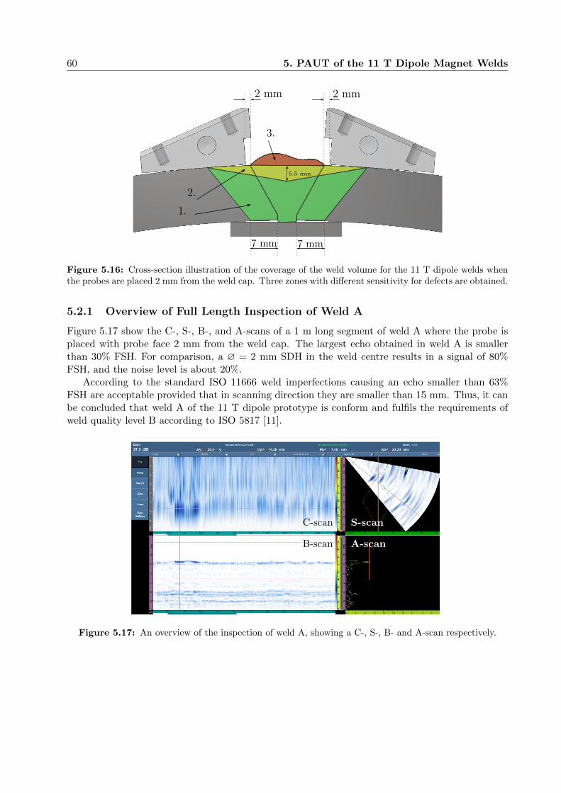
60 5. PAUT of the 11 T Dipole Magnet Welds
3.
2.
1.
5.5 mm
2.
1.
3.
2 mm 2 mm
7 mm 7 mm
Figure 5.16: Cross-section illustration of the coverage of the weld volume for the 11 T dipole welds whenthe probes are placed 2 mm from the weld cap. Three zones with different sensitivity for defects are obtained.
5.2.1 Overview of Full Length Inspection of Weld A
Figure 5.17 show the C-, S-, B-, and A-scans of a 1 m long segment of weld A where the probe isplaced with probe face 2 mm from the weld cap. The largest echo obtained in weld A is smallerthan 30% FSH. For comparison, a ∅ = 2 mm SDH in the weld centre results in a signal of 80%FSH, and the noise level is about 20%.
According to the standard ISO 11666 weld imperfections causing an echo smaller than 63%FSH are acceptable provided that in scanning direction they are smaller than 15 mm. Thus, it canbe concluded that weld A of the 11 T dipole prototype is conform and fulfils the requirements ofweld quality level B according to ISO 5817 [11].
B-scan
C-scan S-scan
A-scan
Figure 5.17: An overview of the inspection of weld A, showing a C-, S-, B- and A-scan respectively.
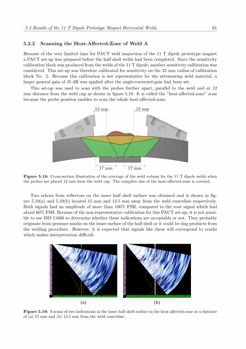
5.2 Results of the 11 T Dipole Prototype Magnet Horizontal Welds 61
5.2.2 Scanning the Heat-Affected-Zone of Weld A
Because of the very limited time for PAUT weld inspection of the 11 T dipole prototype magneta PAUT set-up was prepared before the half shell welds had been completed. Since the sensitivitycalibration block was produced from the welds of the 11 T dipole, another sensitivity calibration wasconsidered. This set-up was therefore calibrated for sensitivity on the 25 mm radius of calibrationblock No. 2. Because this calibration is not representative for the attenuating weld material, alarger general gain of 45 dB was applied after the angle-corrected-gain had been set.
This set-up was used to scan with the probes further apart, parallel to the weld and at 12mm distance from the weld cap as shown in figure 5.18. It is called the ”heat-affected-zone” scanbecause the probe position enables to scan the whole heat-affected-zone.
12 mm 12 mm
17 mm 17 mm
Figure 5.18: Cross-section illustration of the coverage of the weld volume for the 11 T dipole welds whenthe probes are placed 12 mm from the weld cap. The complete size of the heat-affected-zone is covered.
Two echoes from reflectors on the inner half shell surface was obtained and is shown in fig-ure 5.19(a) and 5.19(b) located 15 mm and 13.5 mm away from the weld centreline respectively.Both signals had an amplitude of more than 100% FSH, compared to the root signal which hadabout 60% FSH. Because of the non-representative calibration for this PAUT set-up, it is not possi-ble to use ISO 11666 to determine whether these indications are acceptable or not. They probablyoriginate from pressure marks on the inner surface of the half shell or it could be slag products fromthe welding procedure. However, it is expected that signals like these will correspond to crackswhich makes interpretation difficult.
(a) (b)
Figure 5.19: S-scans of two indications in the inner half shell surface in the heat-affected-zone at a distanceof (a) 15 mm and (b) 13.5 mm from the weld centreline.

62 5. PAUT of the 11 T Dipole Magnet Welds
5.2.3 Scanning Selected Regions of Weld A at High Gain
Increasing the gain to a total of 45 dB enabled more analysis since the subtle amplitude differencesbecomes clearer. Noise and background signals are equally amplified, i.e. one cannot decide if thefound indications are acceptable or not. However it is a cause for further testing of the region,maximizing the signal and perhaps using a different inspection method.
In a section of the weld, the root have melted significantly more than normal and fused to thebacking plate at a wider area as shown in figure 5.20. A comparison between radiography andultrasonic inspection is given. This feature of the weld is seen by both PAUT probes from bothsides of the weld and is approximately 20 cm long.
(a)
(b)
Figure 5.20: The root has fused to a larger area of the backing plate, ≈20 cm. (a) Radiographic image.(b) Corresponding B-scan, the radiographic image show the area between the black lines.
(a)
(b)
Figure 5.21: (a) Picture of the surface with the surface-lack-of-fusion. The arrow indicate the clearestarea, but the whole line is affected. (b) B-scan from the corresponding area.

5.2 Results of the 11 T Dipole Prototype Magnet Horizontal Welds 63
In another section of the weld, a surface-lack-of-fusion (surface-LOF), approximately 30 cmlong was found, shown in and confirmed with a visual inspection shown in figure 5.21(a). The welddid not fuse completely with the parent material at the top surface, which show up clearly in theB-scan in figure 5.21(b). The arrow indicate the clearest spot but the whole line in the image hasthis surface-LOF. It was estimated to have a depth of <0.5 mm.
5.2.4 Scanning Selected Regions in Weld A where Radiography Revealed Pores
The PAUT set-up shown in figure 5.16 that was calibrated for sensitivity with the ∅ = 2 mmSDHs in the 11 T weld sample was used to inspect a region in weld A where a radiography revealedporosity shown in Figure 5.22(a). Their size were approximately 0.8 mm diameter, separated byless than 1 mm. Individually, the maximum size of a pore is 3 mm diameter according to ISO 5817,however since they are so close to each other, they must be considered as one, making this groupof pores unacceptable.
This area of the weld was extensively tested with the PAUT set-up at a very large general gainsetting to be able to distinguish the signal from the pores from the background noise, howeverunsuccessful. After the weld cap was grinded away an ultrasonic test using a 4 MHz longitudinalwave, dual element conventional probe at 0◦ showed that it is possible to detect pores of this size.
After grinding down to the location of the two closely lying pores, their depth below half shellsurface was measured to 2 mm. The ultrasonic beam angle that is required to reach these poreswith the PAUT set-up would be very large, >85◦, if inspected from the side of the ungroundedweld cap, at a sound path of approximately 25 mm. At such large angles there is large attenuation,resulting in bad signal to noise ratio making it hard to distinguish the signal. It may be possibleto detect a pore of this size if the required ultrasonic beam angle is smaller.
(a)
(b)
Figure 5.22: (a) Radiographic image of region of weld A with pores. The single pore at the left side isacceptable. The two closely lying pores on the right form an unacceptable defect. (b) Two exposed closelylying pores 2 mm below shell surface.

64 5. PAUT of the 11 T Dipole Magnet Welds
5.2.5 Scanning Regions in Weld B where a Radiography Revealed Defects
A radiography of a region in weld B revealed three defects which could potentially be LOF, shownin figure 5.24(a). Since LOF is one of the most important type of defect to detect and characterize,this area was tested extensively both using the scanner and manually. The PAUT set-up calibratedon ∅ = 2 mm SDHs in the centreline of an 11 T dipole weld sample was used, however at a largergeneral gain of 40.5 dB.
When scanning the weld with probes parallel to the weld at a 2 mm distance from the weld capas shown in figure 5.16 the defects were not detected. By skewing the probes by 15◦ as shown infigure 5.23, all three defects were detected in one scan as shown in figure 5.24(b). The dependencyof probe angle to receive a strong ultrasonic echo is typical for a flat defect which suggest that thedefects are in fact LOF or crack.
Figure 5.23: Top view illustration of one of the 15◦ skewed probe scans. The scanning direction is alongthe weld, i.e. up or down of the paper.
The root background signals are suppressed to much lower levels when skewing the probescompared to when scanning with probes parallel to the weld which enables the use of a higher gainwithout root signal interference. The noise was below 20% while the defects had a signal amplitudelarger than 100% FSH which made them easy to distinguish. The defects were only detected bythe probe from one side of the weld.
The measured depth of the defects by the PAUT set-up were 16 mm and 15 mm below surface.However due to the probe skew angle on the cylindrical surface, the positioning accuracy of thisscan is estimated to ±2 mm.
Because of the longer sound path distance to the weld region and the worse coupling to thecylindrical surface of the half shells in the skewed probe configuration, a larger general gain must beapplied. The reference sensitivity level for acceptance level according to ISO 11666 is therefore notapplicable. However, as these defects are suspected of being LOF or cracks which is not permittedaccording to ISO 5817, this scan can be used for determining areas which require further testing.
After the weld cap had been removed this area was inspected with one hand-held probe in orderto maximize the signal from the defects. A signal amplitude of 190% FSH was obtained and noiseless than 30% FSH.
Figure 5.24(c) show the exposed defects after grinding down the weld area. Their depthsmeasured 15.1 mm and 14.2 mm below surface using callipers.

5.2 Results of the 11 T Dipole Prototype Magnet Horizontal Welds 65
(a)
(b)
(c)
Figure 5.24: (a) Radiographic image between 290 cm and 300 cm of weld B showing three defects, pre-sumably LOF. (b) B-scan of the same weld volume where the defects appear at the same position. Adifferent point of origin was chosen compared to the radiography. (c) Photography of the exposed defectsafter grinding down the weld area.
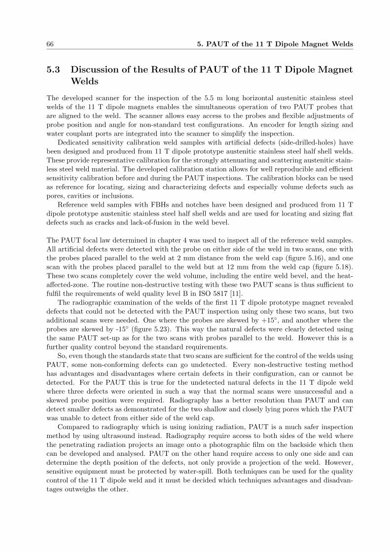
66 5. PAUT of the 11 T Dipole Magnet Welds
5.3 Discussion of the Results of PAUT of the 11 T Dipole MagnetWelds
The developed scanner for the inspection of the 5.5 m long horizontal austenitic stainless steelwelds of the 11 T dipole magnets enables the simultaneous operation of two PAUT probes thatare aligned to the weld. The scanner allows easy access to the probes and flexible adjustments ofprobe position and angle for non-standard test configurations. An encoder for length sizing andwater couplant ports are integrated into the scanner to simplify the inspection.
Dedicated sensitivity calibration weld samples with artificial defects (side-drilled-holes) havebeen designed and produced from 11 T dipole prototype austenitic stainless steel half shell welds.These provide representative calibration for the strongly attenuating and scattering austenitic stain-less steel weld material. The developed calibration station allows for well reproducible and efficientsensitivity calibration before and during the PAUT inspections. The calibration blocks can be usedas reference for locating, sizing and characterizing defects and especially volume defects such aspores, cavities or inclusions.
Reference weld samples with FBHs and notches have been designed and produced from 11 Tdipole prototype austenitic stainless steel half shell welds and are used for locating and sizing flatdefects such as cracks and lack-of-fusion in the weld bevel.
The PAUT focal law determined in chapter 4 was used to inspect all of the reference weld samples.All artificial defects were detected with the probe on either side of the weld in two scans, one withthe probes placed parallel to the weld at 2 mm distance from the weld cap (figure 5.16), and onescan with the probes placed parallel to the weld but at 12 mm from the weld cap (figure 5.18).These two scans completely cover the weld volume, including the entire weld bevel, and the heat-affected-zone. The routine non-destructive testing with these two PAUT scans is thus sufficient tofulfil the requirements of weld quality level B in ISO 5817 [11].
The radiographic examination of the welds of the first 11 T dipole prototype magnet revealeddefects that could not be detected with the PAUT inspection using only these two scans, but twoadditional scans were needed. One where the probes are skewed by +15◦, and another where theprobes are skewed by -15◦ (figure 5.23). This way the natural defects were clearly detected usingthe same PAUT set-up as for the two scans with probes parallel to the weld. However this is afurther quality control beyond the standard requirements.
So, even though the standards state that two scans are sufficient for the control of the welds usingPAUT, some non-conforming defects can go undetected. Every non-destructive testing methodhas advantages and disadvantages where certain defects in their configuration, can or cannot bedetected. For the PAUT this is true for the undetected natural defects in the 11 T dipole weldwhere three defects were oriented in such a way that the normal scans were unsuccessful and askewed probe position were required. Radiography has a better resolution than PAUT and candetect smaller defects as demonstrated for the two shallow and closely lying pores which the PAUTwas unable to detect from either side of the weld cap.
Compared to radiography which is using ionizing radiation, PAUT is a much safer inspectionmethod by using ultrasound instead. Radiography require access to both sides of the weld wherethe penetrating radiation projects an image onto a photographic film on the backside which thencan be developed and analysed. PAUT on the other hand require access to only one side and candetermine the depth position of the defects, not only provide a projection of the weld. However,sensitive equipment must be protected by water-spill. Both techniques can be used for the qualitycontrol of the 11 T dipole weld and it must be decided which techniques advantages and disadvan-tages outweighs the other.

5.3 Discussion of the Results of PAUT of the 11 T Dipole Magnet Welds 67
Due to the anisotropy of the weld material, shown in chapter 4, the sound beam is differentlyattenuated, scattered and diverted when measuring on either side of the weld. This is most clearlyshown in the weld samples which have artificial defects symmetrically around the weld centreline.For example, the SDHs in the centreline of the 11 T dipole weld sample where a difference of 70%FSH (151%-81%) was obtained when measuring the bottom SDHs from either side. As a compari-son the signal amplitude from the bottom SDH in the fusion line weld sample was 114% where thebeam does not pass through any weld material and has similar sound path. This anisotropy causesa sensitivity calibration uncertainty.
Approval of the test procedure for the non-destructive testing of the 11 T dipole welds needs tobe done by an expert with level 3 expertise (table 5.1) within ultrasonic testing according to ISO9712 - Non-destructive testing - Qualification and certification of NDT personnel [56]. Personnelwith expertise of level 2 can perform the routine tests, analyse the data and report the results.
Table 5.1: Minimum requirements for level certification for ultrasonic testing. [56]
Level 1 Level 2 Level 3Training 40 hours 80 hours 40 hours
Industrial experience 3 months 9 months 18 months


6
CONCLUSION
A test setup for the non-destructive testing of the 11 T dipole horizontal welds by PAUT hasbeen developed and commissioned. A scanner that allows to control the welds in a well-definedand reproducible test geometry with two phased array probes aligned to the 5.5 m long horizontalwelds has been designed and built.
Dedicated calibration and reference blocks with artificial defects have been developed and pro-duced. Different focal laws have been compared, and the sensitivity to detect different defect typeshas been determined.
One scan with two phased array probes aligned parallel to the weld in 2 mm distance from theweld cap edge, and one scan with the probes aligned parallel to the weld in 12 mm distance fromthe weld cap edge are sufficient to show if the inspected welds fulfil the requirements of weld qualitylevel B according to ISO 5817 [11].
The standard test duration for the two scans of the two 5.5 m long horizontal welds of the 11 Tdipole magnets is about one day, provided that no defects are found that need to be characterizedin more detail.
Some natural defects were only seen with two additional scans, one with +15◦ and one with-15◦ skewed probes in relation to the weld.
The ultrasonic inspection can be much more sensitive and efficient if the weld cap is removedprior to the weld inspection, so that a direct detection of the entire weld volume with a singleultrasound probe is possible. This can be exploited to examine in more detail defects that havebeen revealed by the PAUT test.
In order to assure a good coupling of the wedges to the steel shells, on 5 cm on either side of thewelds surface irregularities like tack-welds, weld projections and pressure marks must be removedprior to the weld inspection. Water is used as coupling medium, and the surrounding equipmentmust be protected from water spill.
According to ISO 9712, level 2 certification is required for the non-destructive testing of thepressure vessel welds by phased array ultrasonic testing, and level 3 certification is required in orderto approve the test procedure, set-up and equipment [56].
69


Appendices
71

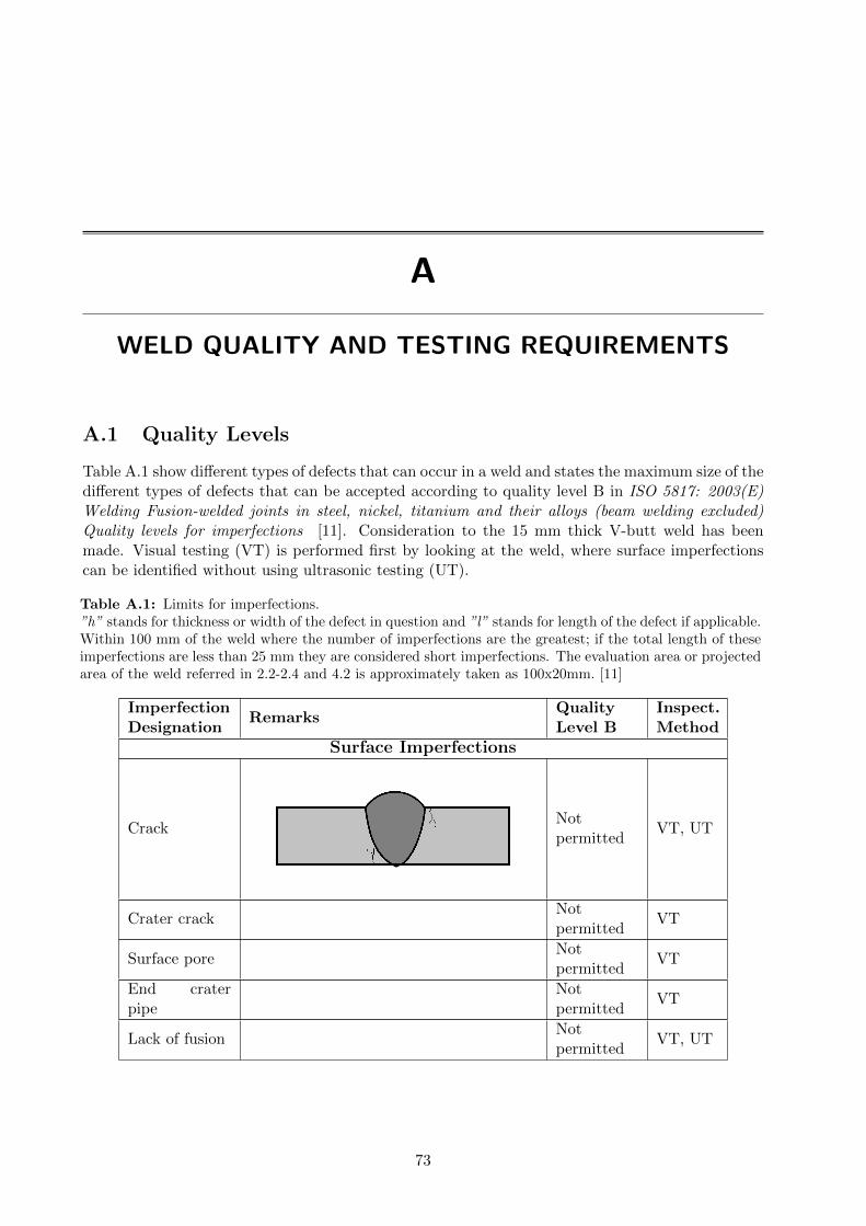
A
WELD QUALITY AND TESTING REQUIREMENTS
A.1 Quality Levels
Table A.1 show different types of defects that can occur in a weld and states the maximum size of thedifferent types of defects that can be accepted according to quality level B in ISO 5817: 2003(E)Welding Fusion-welded joints in steel, nickel, titanium and their alloys (beam welding excluded)Quality levels for imperfections [11]. Consideration to the 15 mm thick V-butt weld has beenmade. Visual testing (VT) is performed first by looking at the weld, where surface imperfectionscan be identified without using ultrasonic testing (UT).
Table A.1: Limits for imperfections.”h” stands for thickness or width of the defect in question and ”l” stands for length of the defect if applicable.Within 100 mm of the weld where the number of imperfections are the greatest; if the total length of theseimperfections are less than 25 mm they are considered short imperfections. The evaluation area or projectedarea of the weld referred in 2.2-2.4 and 4.2 is approximately taken as 100x20mm. [11]
ImperfectionDesignation
RemarksQualityLevel B
Inspect.Method
Surface Imperfections
CrackNotpermitted
VT, UT
Crater crackNotpermitted
VT
Surface poreNotpermitted
VT
End craterpipe
Notpermitted
VT
Lack of fusionNotpermitted
VT, UT
73

74 A. Weld Quality and Testing Requirements
ImperfectionDesignation
RemarksQualityLevel B
Inspect.Method
Incompleteroot penetra-tion
Notpermitted
UT
Continuousundercut andintermittentundercut
h ≤ 0.5mm VT
Shrinkagegroove
Short im-perfections:h ≤ 0.5mm
UT
Excess weldmetal
h ≤ 3mm VT
Excesspenetration
h ≤ 2mm UT
Incorrect weldtoe
α ≥ 150◦ VT
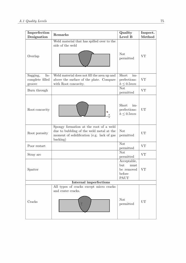
A.1 Quality Levels 75
ImperfectionDesignation
RemarksQualityLevel B
Inspect.Method
Overlap
Weld material that has spilled over to theside of the weld
Notpermitted
VT
Sagging, In-complete filledgroove
Weld material does not fill the area up andabove the surface of the plate. Comparewith Root concavity.
Short im-perfections:h ≤ 0.5mm
VT
Burn throughNotpermitted
VT
Root concavityShort im-perfections:h ≤ 0.5mm
UT
Root porosity
Spongy formation at the root of a welddue to bubbling of the weld metal at themoment of solidification (e.g. lack of gasbacking)
Notpermitted
UT
Poor restartNotpermitted
VT
Stray arcNotpermitted
VT
Spatter
Acceptable,but mustbe removedbeforePAUT
VT
Internal imperfections
Cracks
All types of cracks except micro cracksand crater cracks.
Notpermitted
UT
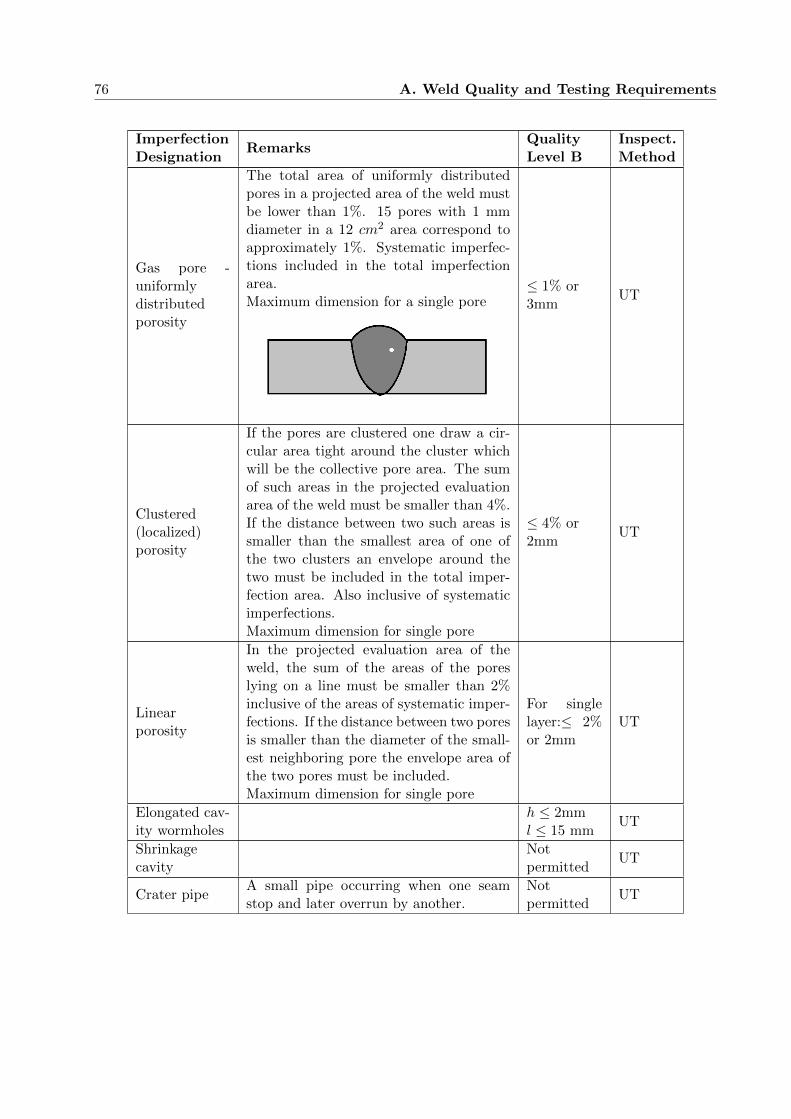
76 A. Weld Quality and Testing Requirements
ImperfectionDesignation
RemarksQualityLevel B
Inspect.Method
Gas pore -uniformlydistributedporosity
The total area of uniformly distributedpores in a projected area of the weld mustbe lower than 1%. 15 pores with 1 mmdiameter in a 12 cm2 area correspond toapproximately 1%. Systematic imperfec-tions included in the total imperfectionarea.Maximum dimension for a single pore
≤ 1% or3mm
UT
Clustered(localized)porosity
If the pores are clustered one draw a cir-cular area tight around the cluster whichwill be the collective pore area. The sumof such areas in the projected evaluationarea of the weld must be smaller than 4%.If the distance between two such areas issmaller than the smallest area of one ofthe two clusters an envelope around thetwo must be included in the total imper-fection area. Also inclusive of systematicimperfections.Maximum dimension for single pore
≤ 4% or2mm
UT
Linearporosity
In the projected evaluation area of theweld, the sum of the areas of the poreslying on a line must be smaller than 2%inclusive of the areas of systematic imper-fections. If the distance between two poresis smaller than the diameter of the small-est neighboring pore the envelope area ofthe two pores must be included.Maximum dimension for single pore
For singlelayer:≤ 2%or 2mm
UT
Elongated cav-ity wormholes
h ≤ 2mml ≤ 15 mm
UT
Shrinkagecavity
Notpermitted
UT
Crater pipeA small pipe occurring when one seamstop and later overrun by another.
Notpermitted
UT

A.1 Quality Levels 77
ImperfectionDesignation
RemarksQualityLevel B
Inspect.Method
Inclusions
Solid inclusions, Slag inclusions, flux in-clusions and oxide inclusions
h ≤ 2mml ≤ 15 mm
UT
Metallicinclusionsother thancopper
h ≤ 2mm UT
Copperinclusions
Notpermitted
UT
Lack of fusion
In these three areas:
• Side wall, see figure• Inter-run• Root
Notpermitted
UT
Imperfections in joint geometry
Linearmisalignment
h ≤ 1.5mm VT
Multiple imperfections
Multipleimperfectionsin any crosssection
Maximumtotal heightof imper-fectionsΣh ≤ 3mm
Notapplicable
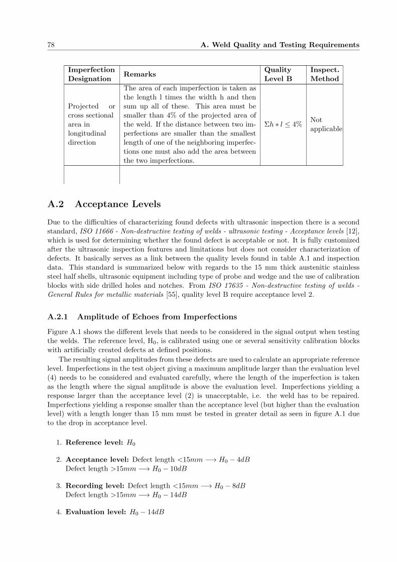
78 A. Weld Quality and Testing Requirements
ImperfectionDesignation
RemarksQualityLevel B
Inspect.Method
Projected orcross sectionalarea inlongitudinaldirection
The area of each imperfection is taken asthe length l times the width h and thensum up all of these. This area must besmaller than 4% of the projected area ofthe weld. If the distance between two im-perfections are smaller than the smallestlength of one of the neighboring imperfec-tions one must also add the area betweenthe two imperfections.
Σh ∗ l ≤ 4%Notapplicable
A.2 Acceptance Levels
Due to the difficulties of characterizing found defects with ultrasonic inspection there is a secondstandard, ISO 11666 - Non-destructive testing of welds - ultrasonic testing - Acceptance levels [12],which is used for determining whether the found defect is acceptable or not. It is fully customizedafter the ultrasonic inspection features and limitations but does not consider characterization ofdefects. It basically serves as a link between the quality levels found in table A.1 and inspectiondata. This standard is summarized below with regards to the 15 mm thick austenitic stainlesssteel half shells, ultrasonic equipment including type of probe and wedge and the use of calibrationblocks with side drilled holes and notches. From ISO 17635 - Non-destructive testing of welds -General Rules for metallic materials [55], quality level B require acceptance level 2.
A.2.1 Amplitude of Echoes from Imperfections
Figure A.1 shows the different levels that needs to be considered in the signal output when testingthe welds. The reference level, H0, is calibrated using one or several sensitivity calibration blockswith artificially created defects at defined positions.
The resulting signal amplitudes from these defects are used to calculate an appropriate referencelevel. Imperfections in the test object giving a maximum amplitude larger than the evaluation level(4) needs to be considered and evaluated carefully, where the length of the imperfection is takenas the length where the signal amplitude is above the evaluation level. Imperfections yielding aresponse larger than the acceptance level (2) is unacceptable, i.e. the weld has to be repaired.Imperfections yielding a response smaller than the acceptance level (but higher than the evaluationlevel) with a length longer than 15 mm must be tested in greater detail as seen in figure A.1 dueto the drop in acceptance level.
1. Reference level: H0
2. Acceptance level: Defect length <15mm −→ H0 − 4dBDefect length >15mm −→ H0 − 10dB
3. Recording level: Defect length <15mm −→ H0 − 8dBDefect length >15mm −→ H0 − 14dB
4. Evaluation level: H0 − 14dB

A.2 Acceptance Levels 79
Figure A.1: Acceptance level diagram with respect to defect length [12].
A.2.2 Grouping of Closely Lying Imperfections
In addition, individually acceptable imperfections with amplitude larger than the recording level arebeing grouped together if the distance between the two imperfections are smaller than a specifiedvalue, different depending on direction, see figure A.2. The grouped imperfections is then againassessed towards figure A.1 using the maximum amplitude of the two and with the total combinedlength. The length of a group shall not be used for further grouping.
Two imperfections are grouped if:
a) dx is less than twice the length of the longer indication
b) dy is smaller than 7.5 mm
c) dz is smaller than 7.5 mm
Example: l1 and l2 are too close, then the combined length is l12 = l1 + l2 + dx
Figure A.2: Grouping of closely lying imperfections. [12]
A.2.3 Limits of the Total Length of Acceptable Indications in a Weld Section
The total cumulative length, lc, of all acceptable indications, individual or grouped, in any lw = 90mm section of the weld, cannot exceed 20%, see figure A.3. This length is given by all single
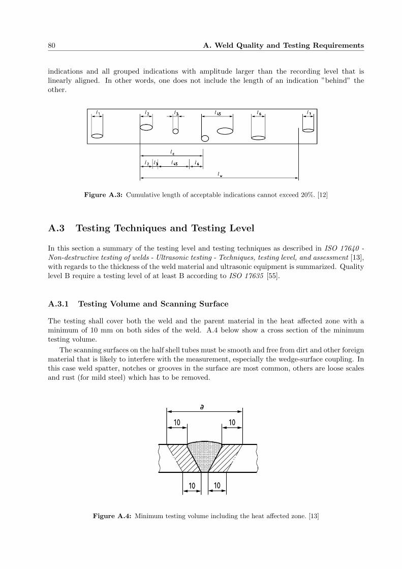
80 A. Weld Quality and Testing Requirements
indications and all grouped indications with amplitude larger than the recording level that islinearly aligned. In other words, one does not include the length of an indication ”behind” theother.
Figure A.3: Cumulative length of acceptable indications cannot exceed 20%. [12]
A.3 Testing Techniques and Testing Level
In this section a summary of the testing level and testing techniques as described in ISO 17640 -Non-destructive testing of welds - Ultrasonic testing - Techniques, testing level, and assessment [13],with regards to the thickness of the weld material and ultrasonic equipment is summarized. Qualitylevel B require a testing level of at least B according to ISO 17635 [55].
A.3.1 Testing Volume and Scanning Surface
The testing shall cover both the weld and the parent material in the heat affected zone with aminimum of 10 mm on both sides of the weld. A.4 below show a cross section of the minimumtesting volume.
The scanning surfaces on the half shell tubes must be smooth and free from dirt and other foreignmaterial that is likely to interfere with the measurement, especially the wedge-surface coupling. Inthis case weld spatter, notches or grooves in the surface are most common, others are loose scalesand rust (for mild steel) which has to be removed.
Figure A.4: Minimum testing volume including the heat affected zone. [13]
A.3 Testing Techniques and Testing Level 81
A.3.2 Range and Sensitivity Settings
The range and sensitivity calibration is performed using the techniques of side-drilled-holes in oneor several specifically designed calibration blocks, and on a standard calibration block. Checks toconfirm the settings shall be performed every 4 hours of testing and at completion of the testingon the same blocks. If a system parameter has changed during the test additional checks must bedone.
If the sensitivity checks reveal a deviation ≤4 dB the sensitivity setting must be corrected beforecontinuing testing. However, if the check show a deviation >4 dB, the setting must be correctedand the testing performed after the previous check has to be repeated. The same goes for rangecalibration where a range deviation of ≤2% shall be corrected before continuing testing. Deviations>2% must be corrected and the previous testing period must be repeated.
A.3.3 Probe Position
Two probe positions are required, one on either side of the weld. If only one side is accessible,two probe angles must be used. The probe position in the axial direction must be recorded inrelation to a reference point on the test piece. The reference point makes it possible to introducea coordinate system where any imperfections in the material can be located.
Since two probes are used simultaneously on both sides of the weld there is no need to usedifferent probe angles, although more angles and/or probe positions will provide more informationwhich could help in the analysis of the PAUT data. By placing the probe wedges with the frontface parallel to the weld axis and as close to the weld crown as possible one can ensure that thewhole weld volume is covered.


B
PAUT EQUIPMENT FOR 11 T DIPOLE WELDINSPECTION
B.1 Main PAUT Equipment
• Omniscan MX2 phased array flaw detector, shown in figure B.1 (a)• 1 Splitter, Omni-A2-Split128, for connecting 2 probes to the Omniscan, shown in figure B.1
(a)• 2 sets of PAUT probes, DMA-4M-16X2-A27, Olympus, shown in figure B.2 (a)• 2 PAUT wedges, SA27-DN55L-FD15-IHC, with 18.7 wedge angle for DMA probes, shown in
figure B.2 (b)• 1 Mini-wheel encoder for length encoding of the acquired PAUT data, shown in figure B.2 (c)• 1 Scanner for double sided PAUT inspection of the horizontal welds of the 11 T dipole, shown
in figure B.3 (a) and figure B.3 (b)• 1 Calibration station for calibration of the PAUT set-up while using the scanner, shown in
figure B.3 (c)• 1 CFU-05 couplant feed unit, water tank, inlet tube with a filter and outlet tube, shown in
figure B.4• 2 T-bar holders for mounting a T-bar on top of the 11 T dipole magnet, shown in figure B.1
(b)• 4 clamps to fix the T-bar holders on top of the 11 T magnet, shown in figure B.1 (b)• 2 Aluminium T-bars, 6.5 m long, 50 mm height, 50 mm width and 5 mm material thickness• 1 Power cable drum with 4 outlets (30 m)• 2 bottles Ultrasonic Gel, Ultragel II, Controltech• 1 Trolley for transport of the PAUT equipment
83
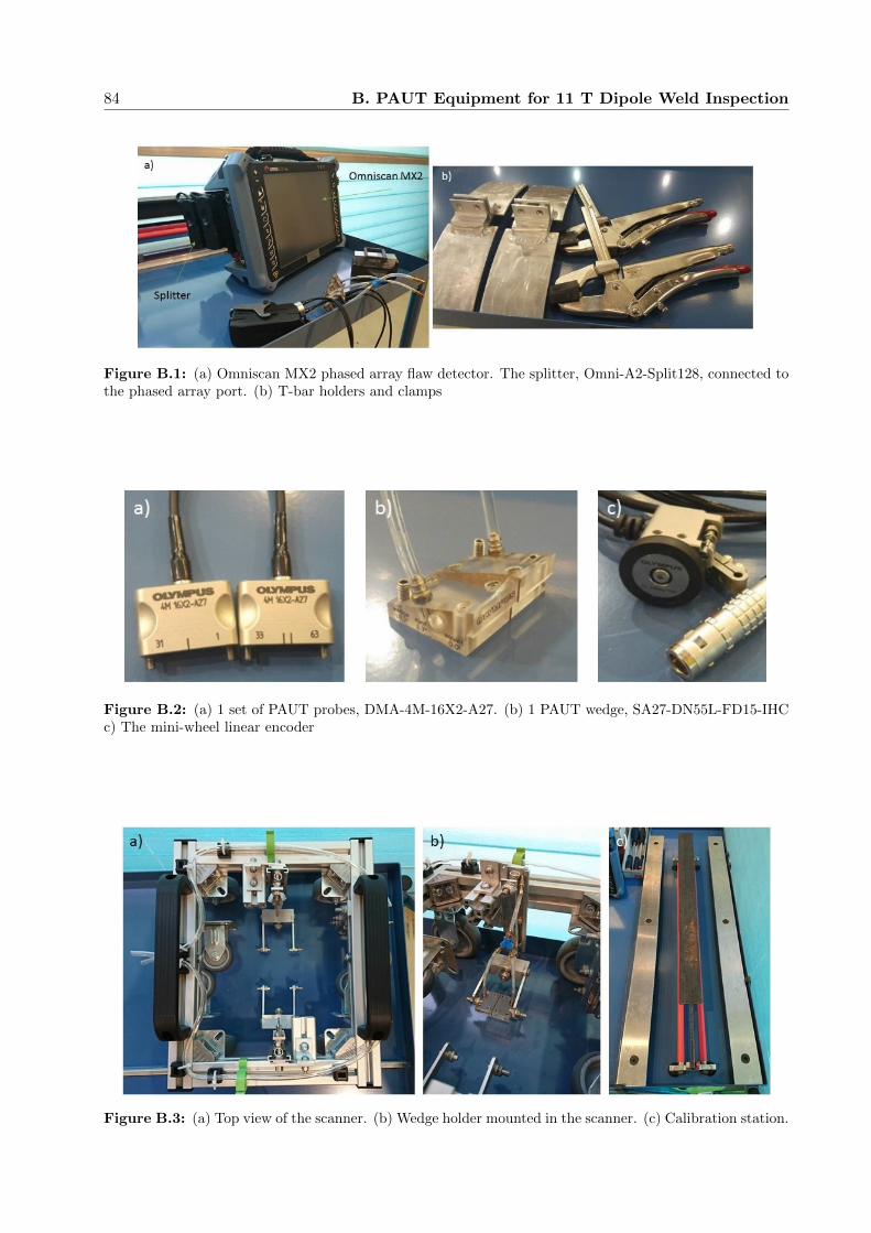
84 B. PAUT Equipment for 11 T Dipole Weld Inspection
Figure B.1: (a) Omniscan MX2 phased array flaw detector. The splitter, Omni-A2-Split128, connected tothe phased array port. (b) T-bar holders and clamps
Figure B.2: (a) 1 set of PAUT probes, DMA-4M-16X2-A27. (b) 1 PAUT wedge, SA27-DN55L-FD15-IHCc) The mini-wheel linear encoder
Figure B.3: (a) Top view of the scanner. (b) Wedge holder mounted in the scanner. (c) Calibration station.
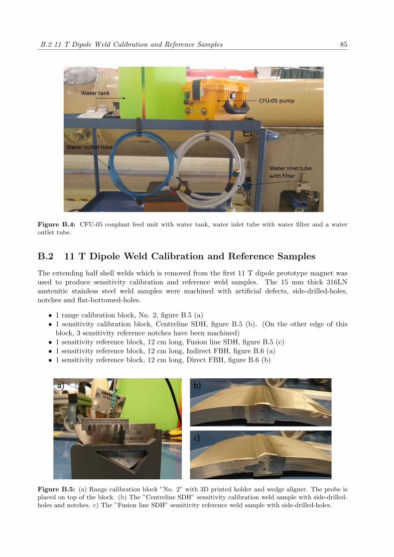
B.2 11 T Dipole Weld Calibration and Reference Samples 85
Figure B.4: CFU-05 couplant feed unit with water tank, water inlet tube with water filter and a wateroutlet tube.
B.2 11 T Dipole Weld Calibration and Reference Samples
The extending half shell welds which is removed from the first 11 T dipole prototype magnet wasused to produce sensitivity calibration and reference weld samples. The 15 mm thick 316LNaustenitic stainless steel weld samples were machined with artificial defects, side-drilled-holes,notches and flat-bottomed-holes.
• 1 range calibration block, No. 2, figure B.5 (a)• 1 sensitivity calibration block, Centreline SDH, figure B.5 (b). (On the other edge of this
block, 3 sensitivity reference notches have been machined)• 1 sensitivity reference block, 12 cm long, Fusion line SDH, figure B.5 (c)• 1 sensitivity reference block, 12 cm long, Indirect FBH, figure B.6 (a)• 1 sensitivity reference block, 12 cm long, Direct FBH, figure B.6 (b)
Figure B.5: (a) Range calibration block ”No. 2” with 3D printed holder and wedge aligner. The probe isplaced on top of the block. (b) The ”Centreline SDH” sensitivity calibration weld sample with side-drilled-holes and notches. c) The ”Fusion line SDH” sensitivity reference weld sample with side-drilled-holes.
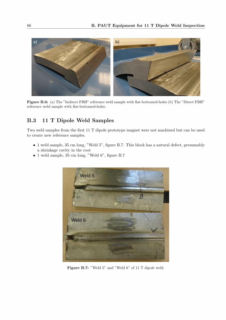
86 B. PAUT Equipment for 11 T Dipole Weld Inspection
Figure B.6: (a) The ”Indirect FBH” reference weld sample with flat-bottomed-holes (b) The ”Direct FBH”reference weld sample with flat-bottomed-holes.
B.3 11 T Dipole Weld Samples
Two weld samples from the first 11 T dipole prototype magnet were not machined but can be usedto create new reference samples.
• 1 weld sample, 35 cm long, ”Weld 5”, figure B.7. This block has a natural defect, presumablya shrinkage cavity in the root• 1 weld sample, 35 cm long, ”Weld 6”, figure B.7
Figure B.7: ”Weld 5” and ”Weld 6” of 11 T dipole weld.

B.4 Other magnet austenitic stainless steel shell weld samples 87
B.4 Other magnet austenitic stainless steel shell weld samples
These weld samples from an LHC main dipole have a MIG weld in 10 mm thick austenitic stainlesssteel half shells, no backing plate. These samples have been machined with artificial defects, side-drilled-holes and root notches.
• 1 weld sample, 7 cm long, SDH block, figure B.8• 1 weld sample, 20 cm long, Notch block, figure B.8
Figure B.8: The two LHC main dipole weld samples are marked with ”SDH block” and ”Notch block”.The four calibration and reference weld samples from the 11 T dipole is also shown.
B.5 16 mm Thick Austenitic Stainless Steel Flat Weld Sample
This 40 cm long and 16 mm thick sample (figure B.9) has five weld areas where artificial defectshave been machined in the parent material. (side-drilled-holes and notches)
Figure B.9: Flat sample with artificial defects machined in five different ”weld areas”.

88 B. PAUT Equipment for 11 T Dipole Weld Inspection
B.6 11 T Single Aperture Short Model Weld Samples
These weld samples from an 11 T single aperture short model are TIG welded and has a backingplate. The austenitic stainless steel half shells are 12 mm thick and the samples has not beenmachined with artificial defects.
• 1 weld sample, 13 cm long, with 3 surface notches, figure B.10• 4 weld samples, 13 cm long, figure B.11
Figure B.10: 1 weld sample from an 11 T single aperture short model with 3 surface notches.
Figure B.11: 4 weld samples from an 11 T single aperture short model without any artificial defects.
B.7 Tools and Attachments
• 2 adjustable spanners• 1 set of Hex-keys• 1 set of Hex-keys with handles• 1 Phillips screwdriver• Attachments for modifications of the scanner
– Screws, lock nuts and washers in M3, M4, M5 and M6 in various sizes.– M6 wing nuts

B.8 Miscellaneous Items 89
– M5 aluminium profile attachments– 4 types of compression springs for wedge holder
B.8 Miscellaneous Items
• 1 Steel T-bar, 1.8 m long, 50 mm height, 50 mm width and 6 mm material thickness forPAUT inspection of horizontal welds on 11 T short models.• 3D-printed parts
– 1 calibration block No. 2 holder with separate piece for wedge alignment, Figure 42 (a)– 7 hooks for trolley in 2 sizes (grey)– 6 aligners for aluminium T-bar (white)– 3 block aligners for steel T-bar (grey)– 1 drainage funnel (green)
• 1 spool transparent water tube, 4 mm inner diameter• 1 bucket• 1 blue paper roll• 8 rolls of plastic bags• 1 roll of red heat shrink tube• 1 roll white duct tape

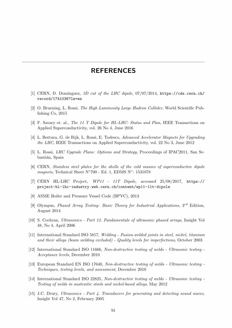
REFERENCES
[1] CERN, D. Dominguez, 3D cut of the LHC dipole, 07/07/2014, https://cds.cern.ch/
record/1741036?ln=en
[2] O. Bruening, L. Rossi, The High Luminosity Large Hadron Collider, World Scientific Pub-lishing Co, 2015
[3] F. Savary et. al., The 11 T Dipole for HL-LHC: Status and Plan, IEEE Transactions onApplied Superconductivity, vol. 26 No 4, June 2016
[4] L. Bottura, G. de Rijk, L. Rossi, E. Todesco, Advanced Accelerator Magnets for Upgradingthe LHC, IEEE Transactions on Applied Superconductivity, vol. 22 No 3, June 2012
[5] L. Rossi, LHC Upgrade Plans: Options and Strategy, Proceedings of IPAC2011, San Se-bastian, Spain
[6] CERN, Stainless steel plates for the shells of the cold masses of superconductive dipolemagnets, Technical Sheet N◦700 - Ed. 1, EDMS N◦: 1531078
[7] CERN HL-LHC Project, WP11 - 11T Dipole, accessed 25/08/2017, https://
project-hl-lhc-industry.web.cern.ch/content/wp11-11t-dipole
[8] ASME Boiler and Pressure Vessel Code (BPVC), 2013
[9] Olympus, Phased Array Testing: Basic Theory for Industrial Applications, 3rd Edition,August 2014
[10] S. Cochran, Ultrasonics - Part 12. Fundamentals of ultrasonic phased arrays, Insight Vol48, No 4, April 2006
[11] International Standard ISO 5817, Welding - Fusion-welded joints in steel, nickel, titaniumand their alloys (beam welding excluded) - Quality levels for imperfections, October 2003
[12] International Standard ISO 11666, Non-destructive testing of welds - Ultrasonic testing -Acceptance levels, December 2010
[13] European Standard EN ISO 17640, Non-destructive testing of welds - Ultrasonic testing -Techniques, testing levels, and assessment, December 2010
[14] International Standard ISO 22825, Non-destructive testing of welds - Ultrasonic testing -Testing of welds in austenitic steels and nickel-based alloys, May 2012
[15] J.C. Drury, Ultrasonics - Part 4. Transducers for generating and detecting sound waves,Insight Vol 47, No 2, February 2005
91

92 REFERENCES
[16] J.C. Drury, Ultrasonics - Part 1. Basic principles of sound, Insight Vol 46, No 11, November2004
[17] F. A. Jenkins, W. W. Watson Huygen’s principle, Access Science, 2014
[18] https://www.nde-ed.org/EducationResources/CommunityCollege/Ultrasonics/
Physics/wavepropagation.htm, Accessed 23-04-2018
[19] J.C. Drury, Ultrasonics - Part 2. Properties of sound waves, Insight Vol 46, No 12, Decem-ber 2004
[20] J.C. Drury, Ultrasonics - Part 3. Refraction and mode conversion, Insight Vol 47, No 1,January 2005
[21] J.C. Drury, Ultrasonics - Part 7. The ultrasonic beam, Insight Vol 47, No 5, May 2005
[22] B. W. Drinkwater, P. D. Wilcox, Ultrasonic arrays for non-destructive evaluation: A re-view, NDT&E International 39 (2006) 525-541
[23] M. Moles, S. Labb’e, Ultrasonic Inspection of Pressure Vessel Construction Welds usingPhased Arrays, www.ndt.net, 3rd MENDT, Middle East Nondestructive Testing Confer-ence & Exhibition, 27-30 Nov 2005, Bahrain, Manama
[24] S. Mahaut, O. Roy, C. Beroni, B. Rotter, Development of phased array techniques toimprove characterization of defect located in a component of complex geometry, Ultrasonics40 (2002) 165-169.
[25] E. Ginzel, Phased Arrays and Mechanised Ultrasonic Testing - A Handbook, Second Edi-tion, Prometheus Press, 2013
[26] S. Baby, T. Balasubramanian, R. J. Pardikar, Ultrasonic study for detection of inner diam-eter cracking in pipeline girth welds using creeping waves, International Journal of PressureVessels and Piping 80 (2003) 139-146
[27] British Institute of Non-Destructive Testing, Creep Waves - High angle ultra-sonic longitudinal waves, http://www.bindt.org/What-is-NDT/Index-of-acronyms/C/Creep-Waves/, accessed 24-04-2018
[28] J. K. Leuk Lai, C. H. Shek, K. H. Lo, Stainless Steel: An Introduction and Their RecentDevelopments, 1st Edition, Bentham Science Publishers, 2012-01-31
[29] S. Sgobba, Materials for high vacuum technology: an overview, CERN, Geneva, Switzerland
[30] D. Klobcar et. al., Active flux tungsten inert gas welding of austenitic stainless steelAISI304, Metalurgija 55 (2016) 4, 617-620
[31] G. Costano, A. Sili, M. E. Tata, Weldability of austenitic stainless steel by metal arcwelding with different shielding gas, Science Direct, Procedia Structural Integrity 2 (2016)3508-3514
[32] D. A. Porter, K. E. Easterling, M. Y. Sherif, Phase Transformations in Metals and Alloys,Third edition, CRC Press Taylor and Francis Group, 2009
[33] M. Moles, S. Righault, Guidelines for Automated Ultrasonic InspectionAustenitic Welds, Olympus, https://www.olympus-ims.com/en/applications/
improved-ut-inspection-austentic-welds/, accessed 25/01/2018

REFERENCES 93
[34] S. Dugan, S. Wagner, Ultrasonic Inspection of Austenitic Stainless Steel Welds with Ar-tificially Produced Stress Corrosion Cracks, AIP Conf. Proc. 1581, 992-998 (2014); doi10.1063/1.4864929
[35] B. Chassignole et. al., Ultrasonic and structural characterization of anisotropic austeniticstainless steel welds: Towards a higher reliability in ultrasonic non-destructive testing,NDT&E International 43, 2010, 273-282
[36] D. Keshun et. al., Varied sub-grain microstructure impacts fracture behaviour and resistancein 316LN weld metal, Engineering Fracture Mechanics 176, 100-115, 2017
[37] D. Keshun, Effect of solution treatment on microstructure and cryogenic toughness of316LN austenite stainless steel weld metal welded by NG-MAG arc welding, Fusion En-gineering and Design 125 (2017) 178-188
[38] C-C. Hsieh, Weite Wu, Overview on Intermetallic Sigma (σ) Phase Precipitation in Stain-less Steels, ISRN Metallurgy, Vol 2012, Article ID 732471, 16p
[39] M. Alali, I. Todd, B.P. Wynne, Through-thickness microstructure and mechanical propertiesof electron beam welded 20 mm thick AISI 316L austenitic stainless steel, Materials $ Design130 (2017) 488-500
[40] A. Perron et. al., Understanding sigma-phase precipitation in a stabilized austenitic stainlesssteel (316Nb) through complementary CALPHAD-based and experimental investigations,Acta Materialia 79 (2014) 16-29
[41] J. M. Vitek, S. A. David, The Sigma Phase Transformation in austenitic Stainless Steels,Welding Research Supplement, 106-111, 1986
[42] V. P. Kujanpaa, Weld Defects in Austenitic Stainless Steel Sheets - Effect of WeldingParameters, Welding Research Supplement, 45-52, 1983
[43] V. P. Kujanpaa, S. A. David, C. L. White, Formation of Hot Cracks in Austenitic StainlessSteel Welds - Solidification Cracking, Welding Research Supplement, 203-212, 1986
[44] Olympus Application Notes, Easy Ultrasonic Phased Array Inspection of Corrosion-resistant Alloys and Dissimilar Weld Materials, https://www.olympus-ims.com/en/
easy-ultrasonic-phased-array-inspection-of-corrosion-resistant-alloys-and-dissimilar-weld-materials/,accessed 25/01/2018
[45] E. Lubeigt et. al., Flaws Detection and Localization in Weld Structure Using the TopologicalEnergy Method, 43rd Ann. Rev. of Prog. in Quant. Non-destr. Eval., Vol 36
[46] European Standard EN 10028-7, Flat products made of steels for pressure purposes - Part7: Stainless steels, August 2008
[47] International ASTM E112-13, Standard Test Methods for Determining Average Grain Size,2013
[48] Ultrasonic Testing (UT) - Welds NDT4, TWI Ltd 2013, rev 3, April 2012
[49] Olympus, Dual Matrix Array for the Inspection of Acoustically Noisy Welds, 11/08/2017,http://www.olympus-ims.com/en/applications/dual-matrix-array-inspection/
[50] Olympus NDT inc. CFU03/CFU05/CFU-PWZ Couplant Feed Unit: User’s Manual,DMTA048-01EN - Revision C, February 2013
94 REFERENCES
[51] International Standard ISO 16811, Non-destructive testing of welds - Ultrasonic testing -Sensitivity and range setting, April 2012
[52] International Standard ISO 7963, Welds in steel - Calibration block No. 2 for ultrasonicexamination of welds, September 1985
[53] International Standard ISO 16827, Non-destructive testing of welds - Ultrasonic testing -Characterization and sizing of discontinuities, April 2012
[54] A. G. Terricabras, C. G. Schon, Characterization of the anisotropic necking in duplexstainless steels with lamellar microstructures, Materials Science & Engineering A 717 (2018)20-25
[55] International Standard ISO 17635, Non-destructive testing of welds - Ultrasonic testing -Techniques, General rules for metallic materials, March 2010
[56] International Standard ISO 9712, Non-destructive testing of welds - Qualification and cer-tification of NDT personnel, June 2012
Related Documents