Phase Space Formulation of Quantum Mechanics · Phase Space Formulation of Quantum Mechanics Tony Bracken Centre for Mathematical Physics and Department of Mathematics University

Phase Space Formulation of Quantum Mechanics

Tony Bracken

Centre for Mathematical Physics

and

Department of Mathematics

University of Queensland

SMFT07, Melbourne, January-February 2007

1

Lecture 1 Introduction:

— from the coordinate representation to the phase space

representation; the Weyl-Wigner transform

Lecture 2 The Wigner function:

— nonpositivity; quantum tomography

Lecture 3 Classical and quantum dynamics:

— the Groenewold operator; semiquantum mechanics

2


• QM has many representations

— coordinate rep, momentum rep, Bargmann rep, Zak’s kq – rep, . . .

— each has its own advantages — most are equivalent

3





• The phase space rep is different in character

— not equivalent to the above

— prominent in recent years for applications to quantum optics,

quantum information theory, quantum tomography, . . .

— also for questions re foundations of QM and classical mechanics (CM)

— QM as a deformation of CM, the nature of the QM-CM interface, . . .

4





• The phase space rep is different in character

— not equivalent to the above

— prominent in recent years for applications to quantum optics,

quantum information theory, quantum tomography, . . .

— also for questions re foundations of QM and classical mechanics (CM)

— QM as a deformation of CM, the nature of the QM-CM interface, . . .

• The development of the theory is associated with a very long list of names: Weyl, Wigner,

von Neumann, Groenewold, Moyal, Takabayasi, Stratonovich, Baker, Berezin, Pool, Berry,

Bayen et al., Shirokov, . . .

Our treatment will necessarily be very selective . . .

5

• Start with some familiar reps of QM, related by unitary transformations.

Consider how we form the coordinate rep for a quantum system with one linear degree of

freedom — dynamical variables q, p.

6




• Start with abstract H: complex Hilbert space of state vectors |ϕ〉, |ψ〉, . . .

— scalar product 〈ϕ|ψ〉.

7






• Introduce generalized eigenvectors of q: q|x〉 = x|x〉

— orthonormal 〈x|y〉 = δ(x− y) and complete∫|x〉〈x| dx = I

8






• Introduce generalized eigenvectors of q: q|x〉 = x|x〉

— orthonormal 〈x|y〉 = δ(x− y) and complete∫|x〉〈x| dx = I

• Define a unitary mapping

H u−→ H′ = L2(C, dx) , |ϕ〉 u−→ ϕ = u|ϕ〉

by setting

ϕ(x) = 〈x|ϕ〉 .

9

• Inverse

|ϕ〉 = u−1ϕ =

∫|x〉〈x|ϕ〉 dx

=

∫ϕ(x)|x〉 dx .

Unitarity is evident — u−1 = u†:

〈ϕ|ψ〉 =

∫〈ϕ|x〉〈x|ψ〉 dx =

∫ϕ(x)∗ψ(x) dx .

10

• Inverse

|ϕ〉 = u−1ϕ =

∫|x〉〈x|ϕ〉 dx

=

∫ϕ(x)|x〉 dx .

Unitarity is evident — u−1 = u†:

〈ϕ|ψ〉 =

∫〈ϕ|x〉〈x|ψ〉 dx =

∫ϕ(x)∗ψ(x) dx .

• In the same way we can form the momentum rep:–

p|p〉 = p|p〉

ϕ = v|ϕ〉 ∈ L2(C, dp) , ϕ(p) = 〈p|ϕ〉

v†ϕ = |ϕ〉 =

∫|p〉ϕ(p) dp

11

• Then the coordinate and momentum reps are also related by a unitary transformation:

ϕ = u|ϕ〉 = uv†ϕ

ϕ(x) =

∫〈x|p〉ϕ(p) dp

— the Fourier Transform: 〈x|p〉 = 1√2πeixp/~

All very familiar — dates back (at least) to Dirac’s book.

12

• Before we move on, consider what happens to operators, e.g. in the coordinate rep:

a −→ a′ = u a u†

(a′ϕ)(x) = (u a u†ϕ)(x) =

∫〈x|a|y〉ϕ(y) dy .

— integral operator with kernel aK(x, y) = 〈x|a|y〉.

Note that

a b −→ u a b u† = u a u† u b u† = a′ b′

— so these unitary transformations preserve the product structure of the algebra of

operators on H

— they define algebra isomorphisms.

13

• To define the phase space rep, we have a different starting point:

Consider T : complex Hilbert space of linear operators a on H s.t.

Tr(a† a) <∞— Hilbert-Schmidt operators

— scalar product ((a, b)) = Tr(a†b)

14

• To define the phase space rep, we have a different starting point:

Consider T : complex Hilbert space of linear operators a on H s.t.

Tr(a† a) <∞— Hilbert-Schmidt operators

— scalar product ((a, b)) = Tr(a†b)

• The importance of T stems from the fact that it contains the density operator (matrix)

ρ(t) =

|ψ(t)〉〈ψ(t)| pure state∑

r pr|ψr(t)〉〈ψr(t)| mixed state

pr > 0 ,∑

r pr = 1

ρ(t)† = ρ(t) , ρ(t) ≥ 0 , Tr(ρ(t)) = 1

15

In fact

((ρ(t), ρ(t))) ≡ Tr(ρ(t)2) ≤ 1 ,

so ρ(t) is in T .

Furthermore, we can calculate the expectation value of any observable a ∈ T as

〈a〉(t) = Tr(ρ(t)a) = ((ρ(t), a)) .

Unfortunately, T does not contain I , q , p , . . .

16

• We overcome this by ‘rigging’ T :

Consider S ⊂ T with S = T . Then T ∗ ⊂ S∗, so

S ⊂ T ≡ T ∗ ⊂ S∗

or, with an abuse of notation,

S ⊂ T ⊂ S∗ Gel′fand triple

Choosing e.g.

S = linear span{|m〉〈n|}in terms of the number states |m〉 for m, n = 0, 1, 2, . . . , it is easy to see that S∗

contains all polynomials in I , q , p .

We can extend the definition of ((., .)) to S∗ in a natural way. Then we can calculate

〈a〉(t) = ((ρ(t), a))

for most observables of interest.

17

Question: Do we need H, the space of state vectors, to do QM, or can we get by with T(or more precisely, with S∗)?

(Berry phase? Charge quantization? ....)

18

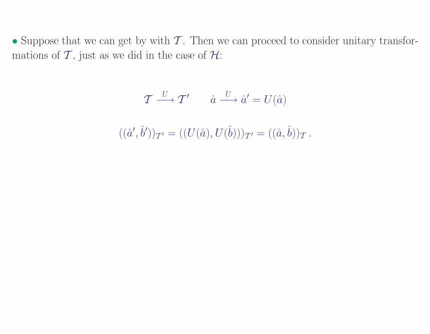
• Suppose that we can get by with T . Then we can proceed to consider unitary transfor-

mations of T , just as we did in the case of H:

T U−→ T ′ aU−→ a′ = U(a)

((a′, b′))T ′ = ((U(a), U(b)))T ′ = ((a, b))T .

19

• Suppose that we can get by with T . Then we can proceed to consider unitary transfor-

mations of T , just as we did in the case of H:

T U−→ T ′ aU−→ a′ = U(a)

((a′, b′))T ′ = ((U(a), U(b)))T ′ = ((a, b))T .

• The previously-defined transformations of operators, induced by transformations of

vectors in H, provide examples:

U(a) = u a u†

((a′, b′))T ′ = Tr(u a u†, u b u†))T ′ = Tr(a, b) = ((a, b))T .

However, it is important to see that not every possible U(a) is of the form u a u†.

20

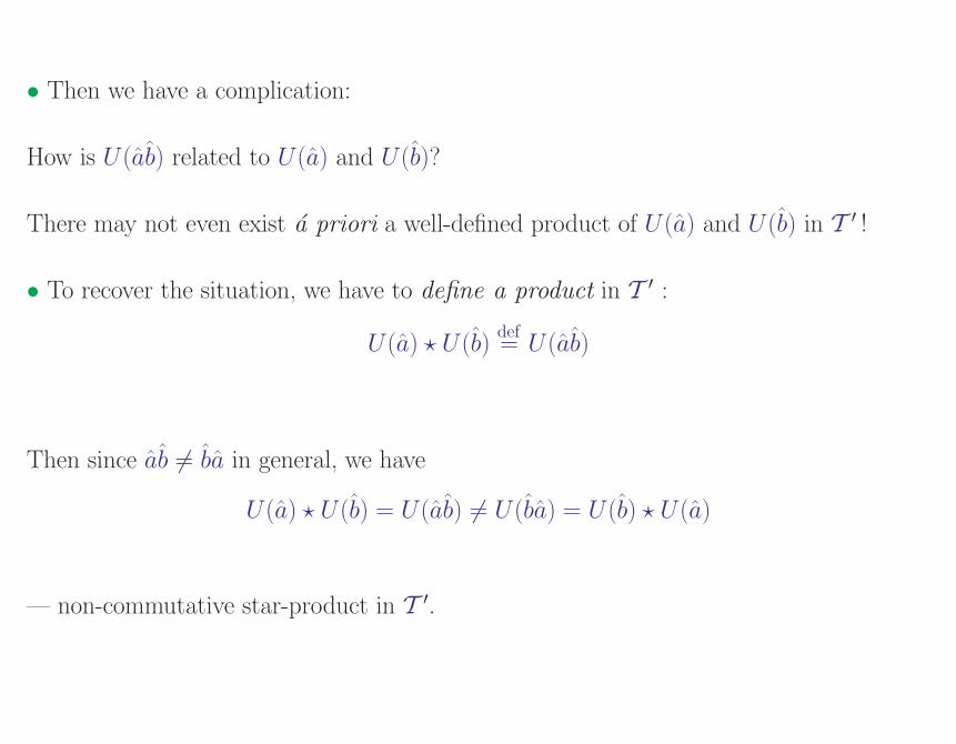
• Then we have a complication:

How is U(ab) related to U(a) and U(b)?

There may not even exist a priori a well-defined product of U(a) and U(b) in T ′ !

21

• Then we have a complication:

How is U(ab) related to U(a) and U(b)?

There may not even exist a priori a well-defined product of U(a) and U(b) in T ′ !

• To recover the situation, we have to define a product in T ′ :

U(a) ? U(b)def= U(ab)

Then since ab 6= ba in general, we have

U(a) ? U(b) = U(ab) 6= U(ba) = U(b) ? U(a)

— non-commutative star-product in T ′.

22

• To set up the unitary U defining the phase space rep, consider the

(hermitian) kernel operator (Stratonovich, 1957)

∆(q, p) = 2P e2i(qp−pq)/~ = 2e−2iqp/~ P e−2ipq/~ e2iqp/~ = 2e2iqp/~ P e2iqp/~ e−2ipq/~

where P is the parity operator: P |x〉 = | − x〉.

23



∆(q, p) = 2P e2i(qp−pq)/~ = 2e2iqp~ P e2iqp/~ e−2ipq/~ = 2e−2iqp~ P e−2ipq/~ e2iqp/~


• The kernel sits in S∗ and defines a continuous generalized basis for T .

Orthonormal:

((∆(q, p), ∆(q′, p′))) = Tr(∆(q, p)†∆(q′, p′)) = 2π~δ(q − q′)δ(p− p′) .

Complete:1

2π~

∫∆(q, p)((∆(q, p), a)) dq dp = a ∀a ∈ T .

24



∆(q, p) = 2P e2i(pq−qp)/~ = 2e2iqp~ P e−2iqp/~ e2ipq/~ = 2e−2iqp~ P e2ipq/~ e−2iqp/~


• The kernel sits in S∗ and defines a continuous generalized basis for T .

Orthonormal:

((∆(q, p), ∆(q′, p′))) = Tr(∆(q, p)†∆(q′, p′)) = 2π~ δ(q − q′) δ(p− p′) .Complete:

1

2π~

∫∆(q, p)((∆(q, p), a)) dq dp = a ∀a ∈ T .

• cf. 〈x|y〉 = δ(x− y) ,∫|x〉〈x|ϕ〉 dx = |ϕ〉 ∀|ϕ〉 ∈ H .

25

• We now define the phase space rep by setting

A(q, p) = ((∆(q, p), a)) = Tr(∆(q, p)†a)

— symbolically, A =W(a) W = Weyl-Wigner transform.

26


A(q, p) = ((∆(q, p), a)) = Tr(∆(q, p)†a)


• Then

((a, b))W−→ 1

2π~

∫A(q, p)∗B(q, p) dq dp ,

so that T ′ = L2(C, dqdp) = K, say.

27


A(q, p) = ((∆(q, p), a)) = Tr(∆(q, p)†a)


• Then

((a, b))W−→ 1

2π~

∫A(q, p)∗B(q, p) dq dp ,

so that T ′ = L2(C, dqdp) = K, say.

• The inverse mapping is

a =W−1(A) =1

2π~

∫∆(q, p)A(q, p) dq dp .

28

• cf.

ϕ(x) = 〈x|ϕ〉

— symbolically, ϕ = u|ϕ〉.

• Then

〈ϕ|ψ〉 u−→∫ϕ(x)∗ψ(x) dx

so that H′ = L2(C, dx).

• The inverse transformation is

|ϕ〉 = u−1ϕ =

∫|x〉ϕ(x) dx .

29

In the case of W , there is a natural product in T ′ = K, namely the ordinary

product of functions A(q, p)B(q, p)

— but clearly this is not the image of ab, because it is commutative.

So in the case of the phase space rep, we will need to use

A ? B =W(ab) 6= AB

(A ? B)(q, p) = ((∆(q, p), ab)) .

30

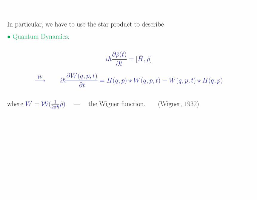
In particular, we have to use the star product to describe

• Quantum Dynamics:

i~∂ρ(t)

∂t= [H, ρ]

W−→ i~∂W (q, p, t)

∂t= H(q, p) ? W (q, p, t)−W (q, p, t) ? H(q, p)

where W =W( 12π~ρ) — the Wigner function. (Wigner, 1932)

31

In particular, we have to use the star product to describe

• Quantum Dynamics:

i~∂ρ(t)

∂t= [H, ρ]

W−→ i~∂W (q, p, t)

∂t= H(q, p) ? W (q, p, t)−W (q, p, t) ? H(q, p)

where W =W( 12π~ρ) — the Wigner function. (Wigner, 1932)

• Quantum symmetries:

a′ = ug a u†g

W−→ Ug(q, p) ? A(q, p) ? Ug(q, p)∗

ug u†g = u†g ug = I ,

W−→ Ug ? U∗g = U ∗g ? Ug = 1 .

— star-unitary representations of groups on phase space. (Fronsdal, 1978)

32

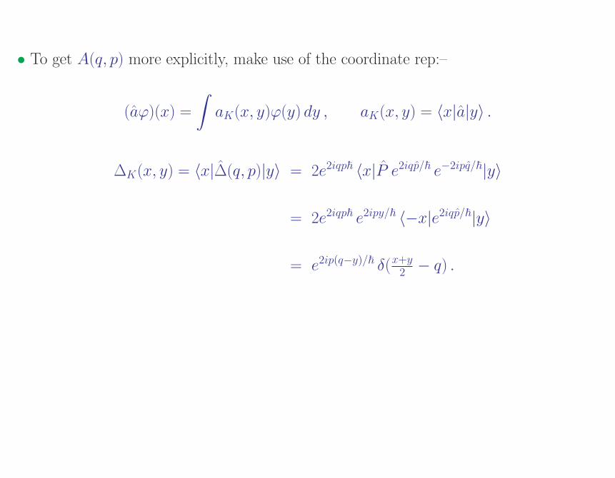
• To get A(q, p) more explicitly, make use of the coordinate rep:–

(aϕ)(x) =

∫aK(x, y)ϕ(y) dy , aK(x, y) = 〈x|a|y〉 .

∆K(x, y) = 〈x|∆(q, p)|y〉 = 2e2iqp~ 〈x|P e2iqp/~ e−2ipq/~|y〉

= 2e2iqp~ e2ipy/~ 〈−x|e2iqp/~|y〉

= e2ip(q−y)/~ δ(x+y2 − q) .

33

• To get A(q, p) more explicitly, make use of the coordinate rep:–

(aϕ)(x) =

∫aK(x, y)ϕ(y) dy , aK(x, y) = 〈x|a|y〉 .

∆K(x, y) = 〈x|∆(q, p)|y〉 = 2e2iqp~ 〈x|P e2iqp/~ e−2ipq/~|y〉

= 2e2iqp~ e2ipy/~ 〈−x|e2iqp/~|y〉

= e2ip(q−y)/~ δ(x+y2 − q) .

• Then

Tr(∆(q, p)a) =

∫〈x|∆(q, p)|y〉〈y|a|x〉 dx dy

=

∫e2ip(q−y)/~ δ(x+y2 − q)aK(y, x) dx dy

i.e. A(q, p) =

∫aK(q − y/2, q + y/2) eipy/~ dy

34

•

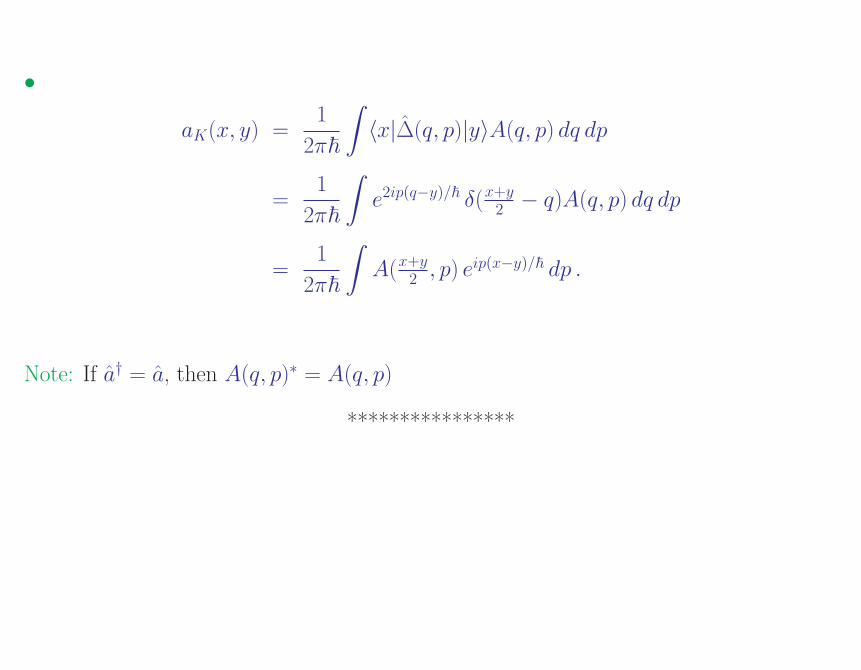
aK(x, y) =1

2π~

∫〈x|∆(q, p)|y〉A(q, p) dq dp

=1

2π~

∫e2ip(q−y)/~ δ(x+y2 − q)A(q, p) dq dp

=1

2π~

∫A(x+y2 , p) eip(x−y)/~ dp .

Note: If a† = a, then A(q, p)∗ = A(q, p)

****************

35

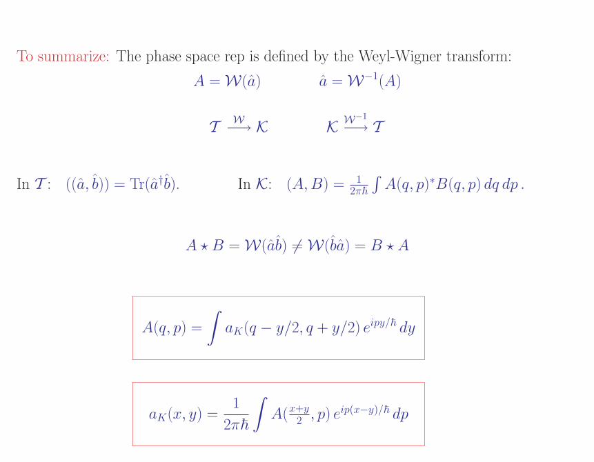
To summarize: The phase space rep is defined by the Weyl-Wigner transform:

A =W(a) a =W−1(A)

T W−→ K K W−1−→ T

In T : ((a, b)) = Tr(a†b). In K: (A,B) = 12π~

∫A(q, p)∗B(q, p) dq dp .

A ? B =W(ab) 6=W(ba) = B ? A

A(q, p) =

∫aK(q − y/2, q + y/2) eipy/~ dy

aK(x, y) =1

2π~

∫A(x+y2 , p) eip(x−y)/~ dp

36

Phase Space Formulation of Quantum Mechanics · Phase Space Formulation of Quantum Mechanics Tony Bracken Centre for Mathematical Physics and Department of Mathematics University

Documents