Rochester Institute of Technology RIT Scholar Works eses esis/Dissertation Collections 6-21-2013 Phase Retrieval using Power Measurements Jamal Arif Follow this and additional works at: hp://scholarworks.rit.edu/theses is esis is brought to you for free and open access by the esis/Dissertation Collections at RIT Scholar Works. It has been accepted for inclusion in eses by an authorized administrator of RIT Scholar Works. For more information, please contact [email protected]. Recommended Citation Arif, Jamal, "Phase Retrieval using Power Measurements" (2013). esis. Rochester Institute of Technology. Accessed from

Welcome message from author
This document is posted to help you gain knowledge. Please leave a comment to let me know what you think about it! Share it to your friends and learn new things together.
Transcript
Rochester Institute of TechnologyRIT Scholar Works
Theses Thesis/Dissertation Collections
6-21-2013
Phase Retrieval using Power MeasurementsJamal Arif
Follow this and additional works at: http://scholarworks.rit.edu/theses
This Thesis is brought to you for free and open access by the Thesis/Dissertation Collections at RIT Scholar Works. It has been accepted for inclusionin Theses by an authorized administrator of RIT Scholar Works. For more information, please contact [email protected].
Recommended CitationArif, Jamal, "Phase Retrieval using Power Measurements" (2013). Thesis. Rochester Institute of Technology. Accessed from
Rochester Institute of Technology
College of Applied Sciences and Technology
Electrical Computer and Telecommunications Engineering Technology (ECTET)
Phase Retrieval using
Power Measurements
Jamal Arif
June 21,2013
Rochester, NewYork, USA
A Research Thesis Submitted in Partial Fulfillment of the Requirements
for the degree of
Masters of Science in Telecommunications Engineering Technology (MSTET)

Thesis Supervisor
Professor Dr.Drew N. Maywar
Department of Telecommunications Technology
College of Applied Sciences and Technology
Rochester Institute of Technology
Rochester, NewYork
Approved by:
Dr. Drew N. Maywar
Thesis Advisor, Department of Electrical and Telecommunications
Engineering Technology.
Professor Mark J. Indelicato
Committee Member, Department of Electrical and Telecommunications
Engineering Technology.
Dr. Miguel Bazdresch
Committee Member, Department of Electrical and Telecommunications
Engineering Technology.
1

Dedicated to my parents..
2
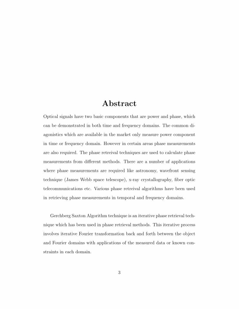
Abstract
Optical signals have two basic components that are power and phase, which
can be demonstrated in both time and frequency domains. The common di-
agonistics which are available in the market only measure power component
in time or frequency domain. However in certain areas phase measurements
are also required. The phase retreival techniques are used to calculate phase
measurements from different methods. There are a number of applications
where phase measurements are required like astronomy, wavefront sensing
technique (James Webb space telescope), x-ray crystallography, fiber optic
telecommunications etc. Various phase retreival algorithms have been used
in retrieving phase measurements in temporal and frequency domains.
Gerchberg Saxton Algorithm technique is an iterative phase retrieval tech-
nique which has been used in phase retrieval methods. This iterative process
involves iterative Fourier transformation back and forth between the object
and Fourier domains with applications of the measured data or known con-
straints in each domain.
3
We worked on developing an iterative phase retrieval technique keeping
Gerchberg Saxton Algorithm as the basis of it and were able to successfully
demonstrate phase retrieval in both temporal and spectral forms for a) Gaus-
sian pulses having a wide range of initial educated guess phase; b) Chirped
Gaussian pulses having various amounts of chirp; c) Chirped Super Gaussian
pulses having various amounts of chirp. A metrics system was defined on
which phase retrieval technique’s success was based showing minimization
of power, phase and instantaneous frequency metrics. During the study we
found that chirped super Gaussian pulses of order 4 converge better than
the chirped Gaussian pulses and also explored a way to choose a good edu-
cational phase without knowledge of the actual phase. Thus, this research
provided a new foundation for further research on phase retrieval techniques
of Gaussian and chirped Gaussian pulses.
4

Acknowledgments
I would like to start in the name of Allah, the most merciful, the most ben-
eficient; for giving me the strength and capability to complete this major
milestone in my life with honor and success.
I would take this opportunity to thank different people who have guided
and supported me throughtout the course of thesis research.
First and Foremost, I want to thank my thesis advisor Professor Drew N.
Maywar for his constant supervision and guidance. It was his continuous sup-
port and encouragement that we were able to complete our thesis research.
I would specially like to thank him for being supportive and patient during
my co-op quarter, and also during the final weeks working with me on some
precise timelines to complete thesis reaserch well before time.
I want to thank Dr. David Aronstein for his inputs in the Gerchberg
Saxton Algorithm and the constant phase offset.
5

I also want to express my gratitude to all the staff, faculty members
of ECTET, my fellow batch mates for their persistent help throughout the
course of my masters degree completion. I want to thank my family and
friends for giving me the love and support throughtout my life.
Finally I would also like to thank my parents and my fiance for believing in
me and supporting me, from coursework completion to thesis research. Their
continuous encouragement made it a lot easier to steer through towards the
completion of the masters degree and thesis research.
6
Contents
1 Introduction 16
1.1 X-Ray Crystallography . . . . . . . . . . . . . . . . . . . . . . 17
1.2 Wavefront Sensing and Phase Retrieval . . . . . . . . . . . . . 17
1.3 Transmission Electron Microscopy . . . . . . . . . . . . . . . . 18
1.4 Fiber Optic Telecommunications . . . . . . . . . . . . . . . . . 19
1.5 Phase Retrieval Technique . . . . . . . . . . . . . . . . . . . . 20
1.6 Overview of Thesis . . . . . . . . . . . . . . . . . . . . . . . . 20
2 Fourier Transform and Gaussian Pulse 22
2.1 Fourier Transform . . . . . . . . . . . . . . . . . . . . . . . . 22
2.2 Analytic Fourier Transform of a Simple Gaussian Pulse . . . . 24
2.3 FFT of a Simple Gaussian Pulse . . . . . . . . . . . . . . . . . 28
2.4 Analytic Fourier Transform of a Complex Gaussian Pulse . . 31
2.5 FFT of a Complex Gaussian Pulse . . . . . . . . . . . . . . . 34
2.6 Inverse Fourier Transform (iFFT) back into temporal Form of
a Gaussian Pulse . . . . . . . . . . . . . . . . . . . . . . . . . 37
2.7 Shift Theorem on Gaussian pulse . . . . . . . . . . . . . . . . 39
7

2.8 Time and Frequency Vector for FFT and iFFT . . . . . . . . 41
3 Phase retrieval technique by Using power Measurements 43
3.1 Phase retrieval technique . . . . . . . . . . . . . . . . . . . . 43
3.2 Establishment of Phase Retrieval Technique . . . . . . . . . . 45
3.2.1 Establishment of Actual Temporal and Spectral Opti-
cal Signals . . . . . . . . . . . . . . . . . . . . . . . . . 45
3.2.2 Establishment of Retrieval Algorithm having Multiple
Iterations . . . . . . . . . . . . . . . . . . . . . . . . . 48
3.2.3 Calculated Temporal Optical Signal . . . . . . . . . . . 50
3.2.4 Calculated Spectral Optical Signal . . . . . . . . . . . 51
3.3 Observations and Issues in Phase Retrieval Technique . . . . . 53
3.3.1 Constant Phase Offset . . . . . . . . . . . . . . . . . . 54
3.3.2 Noise in Calculated Phase Forms . . . . . . . . . . . . 54
3.4 Final Phase Retrieval Technique . . . . . . . . . . . . . . . . . 55
4 Phase Retrieval Technique Metrics 58
4.1 Power Metrics . . . . . . . . . . . . . . . . . . . . . . . . . . . 59
4.1.1 Temporal Power Metric . . . . . . . . . . . . . . . . . 60
4.1.2 Spectral Power Metric . . . . . . . . . . . . . . . . . . 61
4.2 Phase Metrics . . . . . . . . . . . . . . . . . . . . . . . . . . . 63
4.2.1 Temporal Phase Metric . . . . . . . . . . . . . . . . . . 63
4.2.2 Spectral Phase Metric . . . . . . . . . . . . . . . . . . 66
4.3 Instantaneous Frequency Metric . . . . . . . . . . . . . . . . . 69
4.4 Metrics Summary . . . . . . . . . . . . . . . . . . . . . . . . . 72
8
5 Constant Phase Offset in Phase Retrieval Technique 73
5.1 Binary Segmentation Vector . . . . . . . . . . . . . . . . . . . 75
5.1.1 Temporal Power Binary Segmentation Vector . . . . . 76
5.1.2 Spectral Power Binary Segmentation Vector . . . . . . 77
5.2 Constant Phase Offset Removal Technique . . . . . . . . . . . 79
6 Impact of Educated Guess Phase on Phase Retrieval Tech-
nique 82
6.1 Educated Temporal Phase Guess - Narrow Phase Example . . 84
6.2 Educated Temporal Phase Guess - Broad Phase Example . . . 88
6.3 Educated Temporal Phase Guess - Shifted Phase Example . . 91
6.4 Educated Temporal Phase Guess - Shifted Dissimilar Shape
Example . . . . . . . . . . . . . . . . . . . . . . . . . . . . . . 95
7 Phase Retrieval Technique for Chirped Pulses 100
7.1 Defining Chirped Optical Pulse . . . . . . . . . . . . . . . . . 101
7.2 Phase Retrieval on Chirped Pulse . . . . . . . . . . . . . . . . 103
7.3 Metrics of Phase Retrieval on Chirped Pulses . . . . . . . . . 106
7.4 Phase Retrieval Technique on Other Chirped Pulses . . . . . . 109
7.4.1 Phase Retrieval on Chirped Pulse: C = 7 and D = 2 . 110
7.4.2 Retrieval on Chirped Pulse : C = −9 and D = −1 . . . 114
7.5 Sweet Spot for Phase Retrieval technique for Chirped Pulses . 119
8 Phase Retrieval of Chirped Super Gaussian Pulses 122
8.1 Chirped Super Gaussian Pulse . . . . . . . . . . . . . . . . . . 122
9
8.2 Phase retrieval on Chirped Super Gaussian Pulse . . . . . . . 125
8.3 Metrics of Phase Retrieval on Chirped Super Gaussian Pulse . 128
8.3.1 Power Metrics . . . . . . . . . . . . . . . . . . . . . . . 128
8.3.2 Phase Metrics . . . . . . . . . . . . . . . . . . . . . . . 128
8.4 Phase Retrieval on Other chirped Super Gaussian Pulses . . . 129
8.4.1 Chirped Super Gaussian Pulse: C = 16, D = 1 . . . . . 130
8.5 Sweet Spot for Chirped Super Gaussian Pulses . . . . . . . . . 133
10
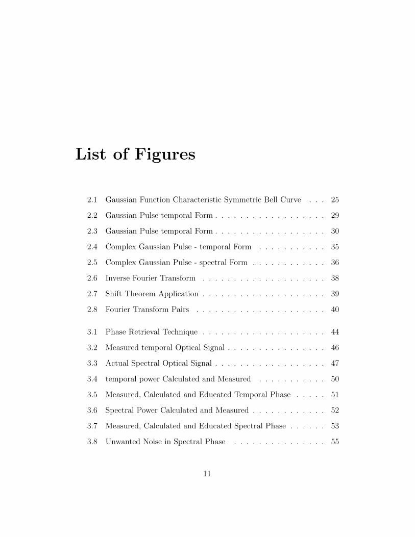
List of Figures
2.1 Gaussian Function Characteristic Symmetric Bell Curve . . . 25
2.2 Gaussian Pulse temporal Form . . . . . . . . . . . . . . . . . . 29
2.3 Gaussian Pulse temporal Form . . . . . . . . . . . . . . . . . . 30
2.4 Complex Gaussian Pulse - temporal Form . . . . . . . . . . . 35
2.5 Complex Gaussian Pulse - spectral Form . . . . . . . . . . . . 36
2.6 Inverse Fourier Transform . . . . . . . . . . . . . . . . . . . . 38
2.7 Shift Theorem Application . . . . . . . . . . . . . . . . . . . . 39
2.8 Fourier Transform Pairs . . . . . . . . . . . . . . . . . . . . . 40
3.1 Phase Retrieval Technique . . . . . . . . . . . . . . . . . . . . 44
3.2 Measured temporal Optical Signal . . . . . . . . . . . . . . . . 46
3.3 Actual Spectral Optical Signal . . . . . . . . . . . . . . . . . . 47
3.4 temporal power Calculated and Measured . . . . . . . . . . . 50
3.5 Measured, Calculated and Educated Temporal Phase . . . . . 51
3.6 Spectral Power Calculated and Measured . . . . . . . . . . . . 52
3.7 Measured, Calculated and Educated Spectral Phase . . . . . . 53
3.8 Unwanted Noise in Spectral Phase . . . . . . . . . . . . . . . 55
11
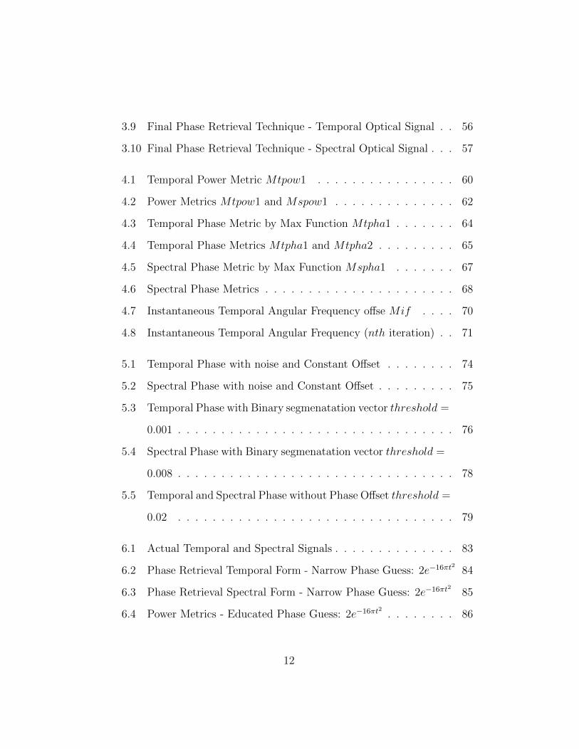
3.9 Final Phase Retrieval Technique - Temporal Optical Signal . . 56
3.10 Final Phase Retrieval Technique - Spectral Optical Signal . . . 57
4.1 Temporal Power Metric Mtpow1 . . . . . . . . . . . . . . . . 60
4.2 Power Metrics Mtpow1 and Mspow1 . . . . . . . . . . . . . . 62
4.3 Temporal Phase Metric by Max Function Mtpha1 . . . . . . . 64
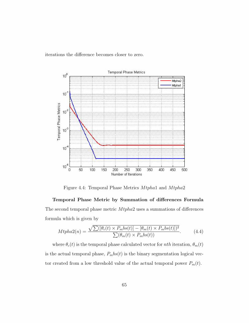
4.4 Temporal Phase Metrics Mtpha1 and Mtpha2 . . . . . . . . . 65
4.5 Spectral Phase Metric by Max Function Mspha1 . . . . . . . 67
4.6 Spectral Phase Metrics . . . . . . . . . . . . . . . . . . . . . . 68
4.7 Instantaneous Temporal Angular Frequency offse Mif . . . . 70
4.8 Instantaneous Temporal Angular Frequency (nth iteration) . . 71
5.1 Temporal Phase with noise and Constant Offset . . . . . . . . 74
5.2 Spectral Phase with noise and Constant Offset . . . . . . . . . 75
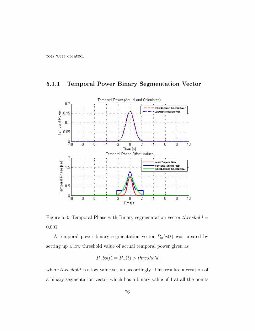
5.3 Temporal Phase with Binary segmenatation vector threshold =
0.001 . . . . . . . . . . . . . . . . . . . . . . . . . . . . . . . . 76
5.4 Spectral Phase with Binary segmenatation vector threshold =
0.008 . . . . . . . . . . . . . . . . . . . . . . . . . . . . . . . . 78
5.5 Temporal and Spectral Phase without Phase Offset threshold =
0.02 . . . . . . . . . . . . . . . . . . . . . . . . . . . . . . . . 79
6.1 Actual Temporal and Spectral Signals . . . . . . . . . . . . . . 83
6.2 Phase Retrieval Temporal Form - Narrow Phase Guess: 2e−16πt2
84
6.3 Phase Retrieval Spectral Form - Narrow Phase Guess: 2e−16πt2
85
6.4 Power Metrics - Educated Phase Guess: 2e−16πt2
. . . . . . . . 86
12
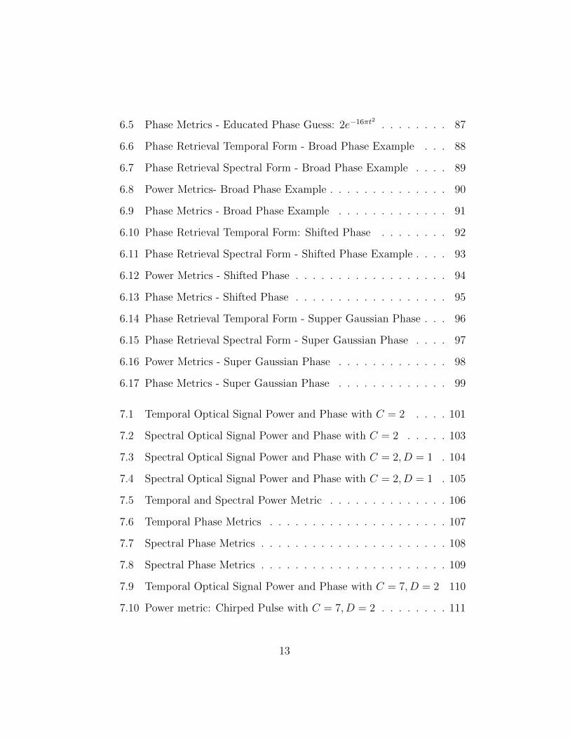
6.5 Phase Metrics - Educated Phase Guess: 2e−16πt2
. . . . . . . . 87
6.6 Phase Retrieval Temporal Form - Broad Phase Example . . . 88
6.7 Phase Retrieval Spectral Form - Broad Phase Example . . . . 89
6.8 Power Metrics- Broad Phase Example . . . . . . . . . . . . . . 90
6.9 Phase Metrics - Broad Phase Example . . . . . . . . . . . . . 91
6.10 Phase Retrieval Temporal Form: Shifted Phase . . . . . . . . 92
6.11 Phase Retrieval Spectral Form - Shifted Phase Example . . . . 93
6.12 Power Metrics - Shifted Phase . . . . . . . . . . . . . . . . . . 94
6.13 Phase Metrics - Shifted Phase . . . . . . . . . . . . . . . . . . 95
6.14 Phase Retrieval Temporal Form - Supper Gaussian Phase . . . 96
6.15 Phase Retrieval Spectral Form - Super Gaussian Phase . . . . 97
6.16 Power Metrics - Super Gaussian Phase . . . . . . . . . . . . . 98
6.17 Phase Metrics - Super Gaussian Phase . . . . . . . . . . . . . 99
7.1 Temporal Optical Signal Power and Phase with C = 2 . . . . 101
7.2 Spectral Optical Signal Power and Phase with C = 2 . . . . . 103
7.3 Spectral Optical Signal Power and Phase with C = 2, D = 1 . 104
7.4 Spectral Optical Signal Power and Phase with C = 2, D = 1 . 105
7.5 Temporal and Spectral Power Metric . . . . . . . . . . . . . . 106
7.6 Temporal Phase Metrics . . . . . . . . . . . . . . . . . . . . . 107
7.7 Spectral Phase Metrics . . . . . . . . . . . . . . . . . . . . . . 108
7.8 Spectral Phase Metrics . . . . . . . . . . . . . . . . . . . . . . 109
7.9 Temporal Optical Signal Power and Phase with C = 7, D = 2 110
7.10 Power metric: Chirped Pulse with C = 7, D = 2 . . . . . . . . 111
13
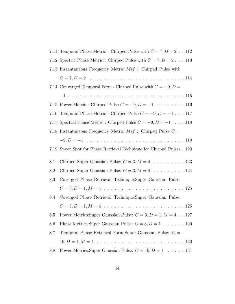
7.11 Temporal Phase Metric : Chirped Pulse with C = 7, D = 2 . . 112
7.12 Spectric Phase Metric : Chirped Pulse with C = 7, D = 2 . . . 113
7.13 Instantaneous Frequency Metric Mif : Chirped Pulse with
C = 7, D = 2 . . . . . . . . . . . . . . . . . . . . . . . . . . . 114
7.14 Converged Temporal Form - Chirped Pulse with C = −9, D =
−1 . . . . . . . . . . . . . . . . . . . . . . . . . . . . . . . . . 115
7.15 Power Metric : Chirped Pulse C = −9, D = −1 . . . . . . . . 116
7.16 Temporal Phase Metric : Chirped Pulse C = −9, D = −1 . . . 117
7.17 Spectral Phase Metric : Chirped Pulse C = −9, D = −1 . . . 118
7.18 Instantaneous Frequency Metric Mif : Chirped Pulse C =
−9, D = −1 . . . . . . . . . . . . . . . . . . . . . . . . . . . . 119
7.19 Sweet Spot for Phase Retrieval Technique for Chirped Pulses . 120
8.1 Chirped Super Gaussian Pulse: C = 3,M = 4 . . . . . . . . . 123
8.2 Chirped Super Gaussian Pulse: C = 3,M = 4 . . . . . . . . . 124
8.3 Coverged Phase Retrieval Technique:Super Gaussian Pulse:
C = 3, D = 1,M = 4 . . . . . . . . . . . . . . . . . . . . . . . 125
8.4 Coverged Phase Retrieval Technique:Super Gaussian Pulse:
C = 3, D = 1,M = 4 . . . . . . . . . . . . . . . . . . . . . . . 126
8.5 Power Metrics:Super Gaussian Pulse: C = 3, D = 1,M = 4 . . 127
8.6 Phase Metrics:Super Gaussian Pulse: C = 3, D = 1 . . . . . . 129
8.7 Temporal Phase Retrieval Form:Super Gaussian Pulse: C =
16, D = 1,M = 4 . . . . . . . . . . . . . . . . . . . . . . . . . 130
8.8 Power Metrics:Super Gaussian Pulse: C = 16, D = 1 . . . . . 131
14

8.9 Power Metrics:Super Gaussian Pulse: C = 16, D = 1 . . . . . 132
8.10 Power Metrics:Super Gaussian Pulse: C = 16, D = 1 . . . . . 134
15
Chapter 1
Introduction
Whenever certain measurements are made in certain instances, phase infor-
mation of the optical field is lost. This phase problem is observed in a number
of different areas and it is desired to calculate the phase of the light signal
as it also contains some necessary information. Phase retrieval is a process
of retrieving the phase of optical signal through certain algorithmic compu-
tational functions, but without directly measuring the phase.
Various algorithms have been applied over the years for phase retrieval.
Phase retrieval methods make use of an educated guess. The algorithm is
carried out several times until the phase converges. This model system is
then compared with the actual optical system having known data patterns,
from which the missing parameters of the optical system can be determined
correctly. It can be further used to calibrate actual optical systems [5].
16
Some of the common areas where phase retrieval methods are employed
are discussed below.
1.1 X-Ray Crystallography
In x-ray crystallography, the crystals are exposed to a beam of x-rays. Inter-
ference is measured and as a result of which unique diffraction patterns are
observed. These diffraction patterns are unique for each crystal. In measure-
ments of these diffracted rays, only intensity measurements are made and
phase measurements, which can be used to specify the atomic positions in
a crystal, are lost in the experiment. Computing phase from these intensity
measurements is desirable and various algorithms have been developed over
the years to calculate phase through phase retrieval techniques [7].
1.2 Wavefront Sensing and Phase Retrieval
Wavefront can be described as a combination of points that have same prop-
erties for instance a combination of points having same phase. Wavefront
sensors are developed in order to measure the wavefront irregularities that
are found in an optical system which can relate to the quality of that optical
system [5].
Wavefront sensing techniques along with phase retrieval algorithms were
employed in the Hubble telescope initially to work on the wavefront aber-
17
rations found in the telescope. Blurred images which were collected by the
Hubble telescope were corrected by the help of wavefront sensing techniques
using phase retrieval methods [5].
The same technology is also being planned by NASA to be used in the
James Webb Space Telescope (JWST to be launched in 2018). JWST con-
sists of a large mirror, i.e. 6.6 meters in diameter, which cant be sent in
space fully open. Therefore it will be folded and opened in outer space.
There are 18 hexagonal segments of the mirror which will unfold accurately
to their positions in the outer space. This would be accomplished by using an
image-based wave front sensing technique employing various phase retrieval
algorithms [5].
1.3 Transmission Electron Microscopy
Transmission Electron microscopy is a technique which is commonly used in
biological sciences and in physics. It is used to examine extremely fine de-
tail of a subject in question. It uses a beam of electrons that is transmitted
through the sample; the beam of electrons interacts as it passes through the
sample and as a result an image is formed. This image is then magnified
and is then focused onto any imaging device. Some information of the image
magnified is lost in between which can be reconstructed using various phase
retrieval methods. In most cases discussed above, phase retrieval work has
been done in space and with spatial frequency [3].
18

1.4 Fiber Optic Telecommunications
A time dependent phase corresponds to a variation in instantaneous temporal
frequency, known as chirp and expressed as
ωi =dθ
dt
where ωi is the instantaneous temporal angular frequency and θ is the
temporal phase. Chirp is often a problem because it leads to wide pulse
spreading via chromatic dispersion. So chirp characteristics are important.
Furthermore, the most advanced fiber-optic telecom systems use phase
modulation to encode data. For instance, Quadrature Phase Shift Keying
(QPSK) is used to achieve 100 Gb/s in the most advanced commercial sys-
tems. So it is important to have phase information.
However, the two most common diagnostics are the optical spectrum
analyzers (OSAs) and photodiode-oscilloscope used in telecommunications.
Neither common diagnostic measures the temporal phase of the optical sig-
nal. Because these diagnostics are common, we seek to use them as the basis
of phase retrieval.
19
1.5 Phase Retrieval Technique
A number of different areas are discussed in the background section providing
an insight to applications of phase retrieval in certain areas. Phase retrieval
techniques have also been applied in astronomy.
In a number of these areas for instance in electron microscopy, wave front
sensing, astronomy, crystallography, and in other fields most of the cases
only intensity measurements are made however as discussed above one wants
to recover phase. One of the approaches which has been quiet successful is
to use the Gerchberg-Saxton algorithm, which is an iterative phase retrieval
technique [3].
The iterative algorithm involves iterative Fourier transformation back and
forth between the object and Fourier domains and application of the mea-
sured data or known constraints in each domain [3]. The iterative technique
of Gerchberg-Saxton, sometimes known as error-reduction algorithm, has
been used in a number of phase retrieval areas discussed in References [8],
[10] and [9].
1.6 Overview of Thesis
An iterative phase retrieval technique is established in the MATLAB envi-
ronment using Gerchberg-Saxton technique as the basis of it. The phase
20
retrieval technique established uses temporal and spectral power measure-
ments to retrieve the phase. Gaussian pulses are chosen to be tested on
the phase retrieval technique because of their unique behavior under going
Fourier transform. A brief overview of thesis documentation is given below.
In chapter 2 a Gaussian pulse is analytically Fourier transformed and
the unique behavior of Gaussian pulses is shown. A Gaussian pulse when
undergoes a Fourier transform, it gives another Gaussian pulse. Time and
frequency vectors are also defined for temporal and spectral forms. In chapter
3 a phase retrieval technique is established using the Gerchberg-Saxton iter-
ative approach as its basis. In chapter 4 metrics are defined which measure
the progress of the phase retrieval technique.
In later chapters a number of new areas are researched upon. In chapter
5, a binary segmentation vector technique is applied on the phase retrieval
technique to have a better phase convergence. The improved phase retrieval
technique is tested with a wide range of educated temporal phase guesses in
chapter 6 and it is shown that the phase retrieval technique works in all cases.
In the last two chapters, chapter 7 and 8, chirped pulses are studied.
The phase retrieval technique is applied on chirped Gaussian and chirped
super Gaussian pulses and some conclusions are made showing that phase
retrieval technique works for chirped Gaussian and super Gaussian pulses in
a particular range of educated temporal phase guesses.
21

Chapter 2
Fourier Transform and
Gaussian Pulse
2.1 Fourier Transform
The Fourier Transform has been named after Joseph Fourier. The Fourier
Transform is a mathematical transform that has found extensive applications
in fields of physics and engineering.
The Fourier transform is a study that is driven by the study of Fourier
series. In Fourier series we observe how any periodic function can be written
as a sum of simple sinusoids. The same concept is applied and drawn-out for
the Fourier Transform, which is applied on non-periodic functions.
The Fourier Transform is a mathematical transform function which in
22
common terms transforms a mathematical function having arguments in
time (a time-domain function) to a function having arguments in frequency
(a frequency-domain function). This new function now created after being
transformed from a time-domain function is known as the Fourier Transform
of the original time-domain function. There are a number of conventions
according to which a Fourier Transform is defined. The Following is one way
of defining Fourier transform.
Consider a time-domain function f(t) (which can be a complex or a real-
valued function) then its Fourier Transform F (s) is given as
F{f(t)}(s) = F (s) =
∞∫−∞
f(t)e−i2πstdt. (2.1)
Where the variable t is defined as time (with units in seconds) and the trans-
form variable s is the frequency (with units in Hertz). This is also commonly
known as Forward Fourier Transform. In most cases F (s) is a complex valued
function and this complex value provides information for both the amplitude
and the phase of the resultant frequency components.
We can also perform an inverse Fourier Transform to get the actual func-
tion f(t) from its Fourier Transform F (s).
The inverse Fourier Transform is given as
F−1{F (s)}(t) = f(t) =
∞∫−∞
F (s)ei2πstds. (2.2)
23
In both equations i =√−1. The functions f(t) and its Fourier Transform
F (s) are known as Fourier Transform Pairs as both can be obtained by the
Fourier Transform and Inverse Fourier Transform. The Following notation
is generally used to show that both of these functions are Fourier Transform
Pairs.
f(t)⇔ F (s)
2.2 Analytic Fourier Transform of a Simple
Gaussian Pulse
A Gaussian Pulse is of the form
f(x) = ae
−(x− b)2
2c2 . (2.3)
where a, b, c are real constants. The Gaussian pulse provides a characteristic
graph which is in the form of a symmetric bell curve. In this symmetric bell
curve a provides the height of this curve, b gives the position of the center of
the peak and c provides the information about the width of the bell curve. A
symmetric bell curve of the the Gaussian pulse is shown in Figure 2.1. To un-
derstand the behavior of a Fourier Transform on a Gaussian pulse, a Fourier
Transform would be applied on the following simple form of a Gaussian pulse.
A simple Gaussian function in time t is expressed as
f(t) = e−πt2
24
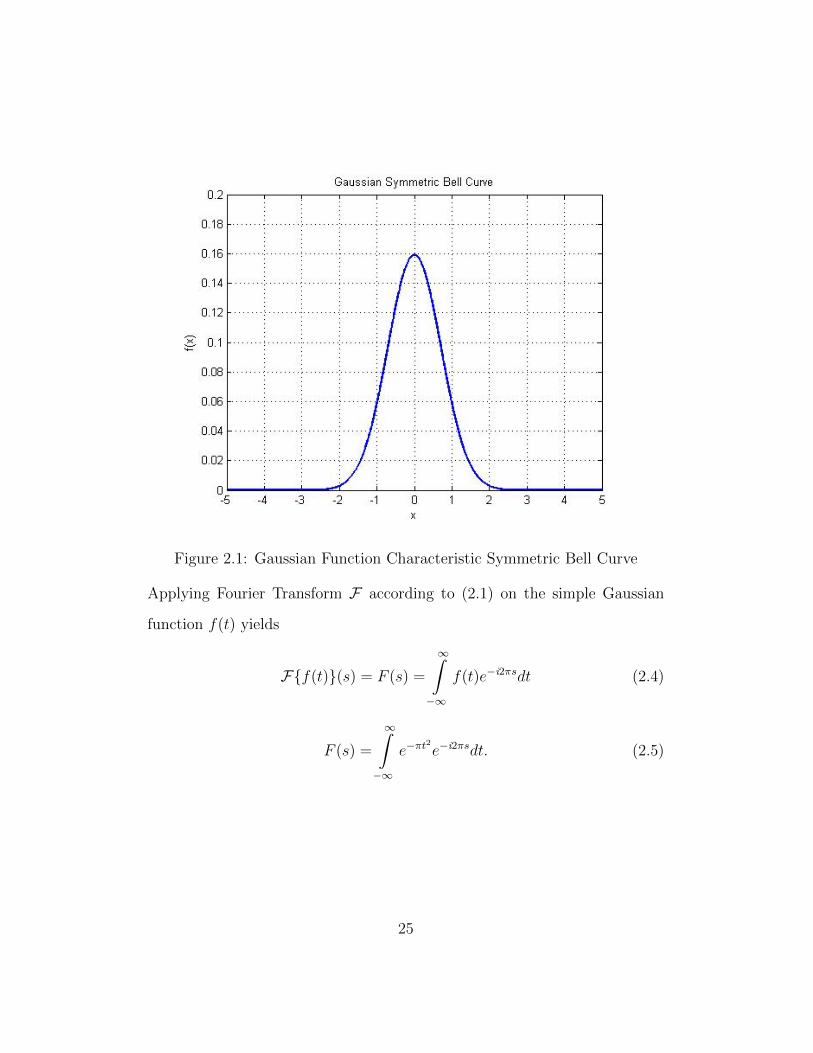
Figure 2.1: Gaussian Function Characteristic Symmetric Bell Curve
Applying Fourier Transform F according to (2.1) on the simple Gaussian
function f(t) yields
F{f(t)}(s) = F (s) =
∞∫−∞
f(t)e−i2πsdt (2.4)
F (s) =
∞∫−∞
e−πt2
e−i2πsdt. (2.5)
25
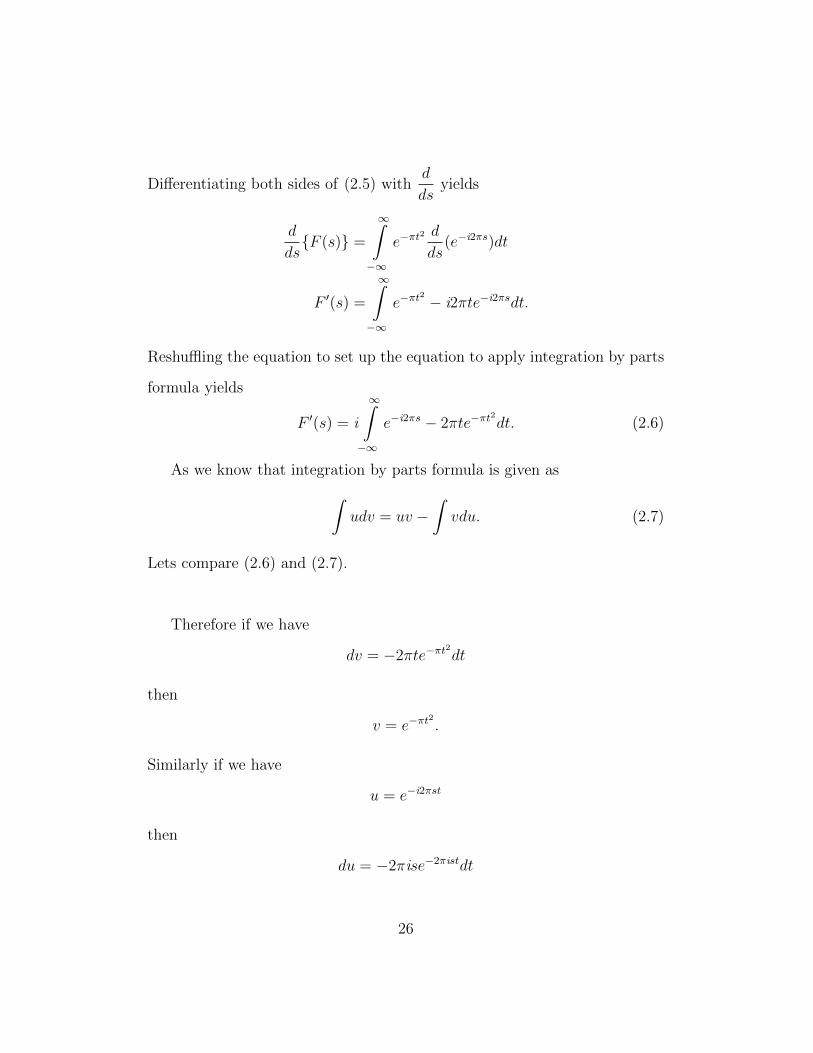
Differentiating both sides of (2.5) withd
dsyields
d
ds{F (s)} =
∞∫−∞
e−πt2 d
ds(e−i2πs)dt
F ′(s) =
∞∫−∞
e−πt2 − i2πte−i2πsdt.
Reshuffling the equation to set up the equation to apply integration by parts
formula yields
F ′(s) = i
∞∫−∞
e−i2πs − 2πte−πt2
dt. (2.6)
As we know that integration by parts formula is given as∫udv = uv −
∫vdu. (2.7)
Lets compare (2.6) and (2.7).
Therefore if we have
dv = −2πte−πt2
dt
then
v = e−πt2
.
Similarly if we have
u = e−i2πst
then
du = −2πise−2πistdt
26
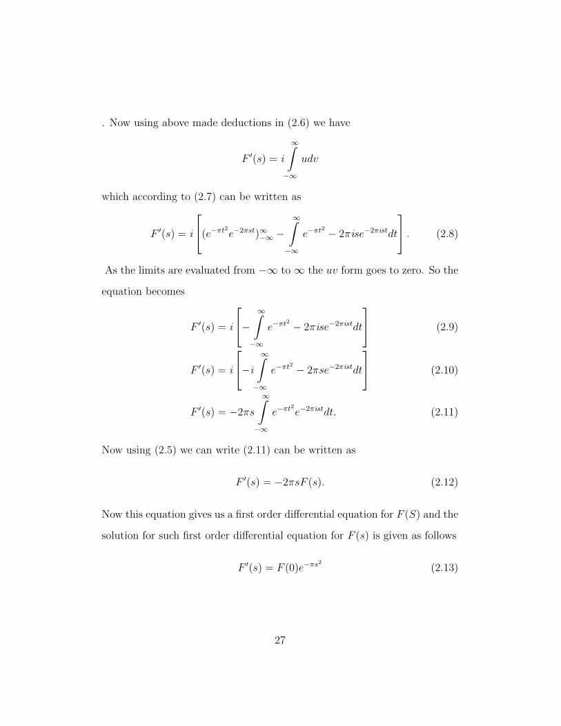
. Now using above made deductions in (2.6) we have
F ′(s) = i
∞∫−∞
udv
which according to (2.7) can be written as
F ′(s) = i
(e−πt2
e−2πst)∞−∞ −∞∫
−∞
e−πt2 − 2πise−2πistdt
. (2.8)
As the limits are evaluated from −∞ to∞ the uv form goes to zero. So the
equation becomes
F ′(s) = i
− ∞∫−∞
e−πt2 − 2πise−2πistdt
(2.9)
F ′(s) = i
−i ∞∫−∞
e−πt2 − 2πse−2πistdt
(2.10)
F ′(s) = −2πs
∞∫−∞
e−πt2
e−2πistdt. (2.11)
Now using (2.5) we can write (2.11) can be written as
F ′(s) = −2πsF (s). (2.12)
Now this equation gives us a first order differential equation for F (S) and the
solution for such first order differential equation for F (s) is given as follows
F ′(s) = F (0)e−πs2
(2.13)
27
where we have
F (0) =
∞∫−∞
e−πt2
e−2πi0tdt (2.14)
F (0) =
∞∫−∞
e−πt2
dt. (2.15)
As according to Eulers Identity we know that
∞∫−∞
e−πt2
dt = 1
therefore
F (0) = 1. (2.16)
Putting value of F (0) in (2.13) we have
F (s) = e−πs2
. (2.17)
Therefore (2.17) shows that Fourier Transform of a Gaussian pulse is another
Gaussian pulse.
F{f(t)}(s) = F (s) = e−πs2
. (2.18)
2.3 FFT of a Simple Gaussian Pulse
In the last section it was shown analytically that Fourier Transform of a
simple Gaussian pulse (time domain) results in a Gaussian pulse in the fre-
quency/spectral domain. The same characteristic of a Gaussian pulse was
applied in the MATLAB environment to check if the MATLAB results are
28
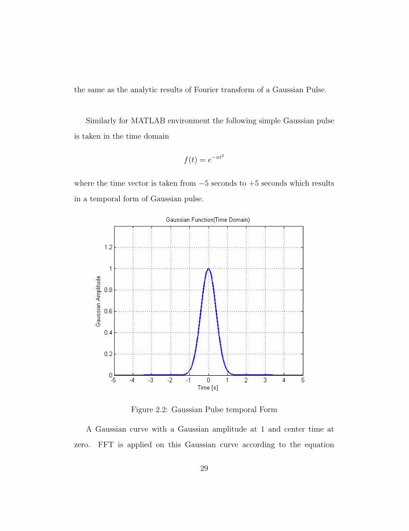
the same as the analytic results of Fourier transform of a Gaussian Pulse.
Similarly for MATLAB environment the following simple Gaussian pulse
is taken in the time domain
f(t) = e−πt2
where the time vector is taken from −5 seconds to +5 seconds which results
in a temporal form of Gaussian pulse.
Figure 2.2: Gaussian Pulse temporal Form
A Gaussian curve with a Gaussian amplitude at 1 and center time at
zero. FFT is applied on this Gaussian curve according to the equation
29
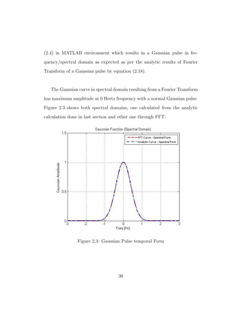
(2.4) in MATLAB environment which results in a Gaussian pulse in fre-
quency/spectral domain as expected as per the analytic results of Fourier
Transform of a Gaussian pulse by equation (2.18).
The Gaussian curve in spectral domain resulting from a Fourier Transform
has maximum amplitude at 0 Hertz frequency with a normal Gaussian pulse.
Figure 2.3 shows both spectral domains, one calculated from the analytic
calculation done in last section and other one through FFT.
Figure 2.3: Gaussian Pulse temporal Form
30
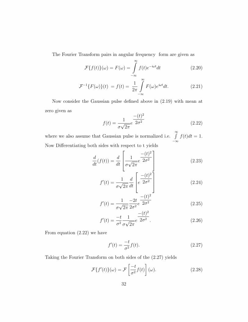
2.4 Analytic Fourier Transform of a Complex
Gaussian Pulse
In previous sections, a simple Gaussian pulse was taken with its mean at
zero. However in this section, a relatively complex Gaussian pulse form is
taken which takes into effect its variance and mean factor into consideration
as well and a Fourier Transform is applied on it.
Consider following Gaussian pulse
f(t) =1
σ√
2πe
−(t− µ)2
2σ2 (2.19)
where parameter µ is the mean of the Gaussian pulse, the parameter σ2 con-
trols the width of the Gaussian characteristic bell curve and is therefore the
variance and σ becomes the standard deviation.
As discussed in previous sections, the Fourier transform is defined in dif-
ferent forms. Previously a simple Gaussian function f(t) in time domain was
transformed into another Gaussian function in frequency domain F (s). In
this section the Fourier Transform given in angular frequency ω would be
applied on a Gaussian distribution function defined above in equation (2.19).
31
The Fourier Transform pairs in angular frequency form are given as
F{f(t)}(ω) = F (ω) =
∞∫−∞
f(t)e−iωtdt (2.20)
F−1{F (ω)}(t) = f(t) =1
2π
∞∫−∞
F (ω)eiωtdt. (2.21)
Now consider the Gaussian pulse defined above in (2.19) with mean at
zero given as
f(t) =1
σ√
2πe
−(t)2
2σ2 (2.22)
where we also assume that Gaussian pulse is normalized i.e.∞∫−∞
f(t)dt = 1.
Now Differentiating both sides with respect to t yields
d
dt(f(t)) =
d
dt
1
σ√
2πe
−(t)2
2σ2
(2.23)
f ′(t) =1
σ√
2π
d
dt
e−(t)2
2σ2
(2.24)
f ′(t) =1
σ√
2π
−2t
2σ2e
−(t)2
2σ2 (2.25)
f ′(t) =−tσ2
1
σ√
2πe
−(t)2
2σ2 . (2.26)
From equation (2.22) we have
f ′(t) =−tσ2f(t). (2.27)
Taking the Fourier Transform on both sides of the (2.27) yields
F{f ′(t)}(ω) = F[−tσ2f(t)
](ω). (2.28)
32
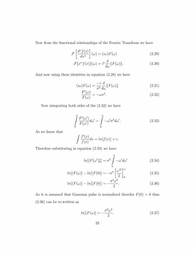
Now from the functional relationships of the Fourier Transform we have
F[dnf(x)
dxn
](ω) = (iω)F (ω) (2.29)
F{xnf(x)}(ω) = ind
dω{F (ω)}. (2.30)
And now using these identities in equation (2.28) we have
(iω)F (ω) =−iσ2
d
dω{F (ω)} (2.31)
F ′(ω)
F (ω)= −ωσ2. (2.32)
Now integrating both sides of the (2.32) we have
ω∫0
F ′(ω′)
F (ω′)dω′ =
ω∫0
−ω′σ2dω′. (2.33)
As we know that ∫f ′(x)
f(x)dx = ln[f(x)] + c.
Therefore substituting in equation (2.33) we have
ln[(F (ω′)]ω0 = σ2
ω∫0
−ω′dω′ (2.34)
ln[(F (ω)]− ln[(F (0)] = −σ2
[ω′2
2
]ω0
(2.35)
ln[(F (ω)]− ln[(F (0)] = −σ2ω2
2. (2.36)
As it is assumed that Gaussian pulse is normalized therefor F (0) = 0 thus
(2.36) can be re-written as
ln[(F (ω)] = −σ2ω2
2. (2.37)
33
Now the equation can be written as follows if we apply exponential at
both sides
eln[f(ω)] = e−σ2ω2
2 (2.38)
F (ω) = e−σ2ω2
2 . (2.39)
Equation (2.39) shows that Fourier Transform (angular frequency form ω) of
a complex Gaussian pulse is another Gaussian pulse as well.
Now we can re-write equation (2.21) as
F{ 1
σ√
2πe
−(t)2
2σ2 }(ω) = F (ω) = e−σ2ω2
2 . (2.40)
This shows that Fourier Transform of a Gaussian pulse is another Gaus-
sian pulse. The same would be now shown in MATLAB environment that
FFT of a Gaussian pulse is another Gaussian pulse.
2.5 FFT of a Complex Gaussian Pulse
In the last section a complex form of Gaussian was taken and it was shown
analytically that Fourier Transform of a Gaussian pulse is another Gaussian.
The same characteristic would be shown in MATLAB environment and
analytic results would be checked in MATLAB.
34
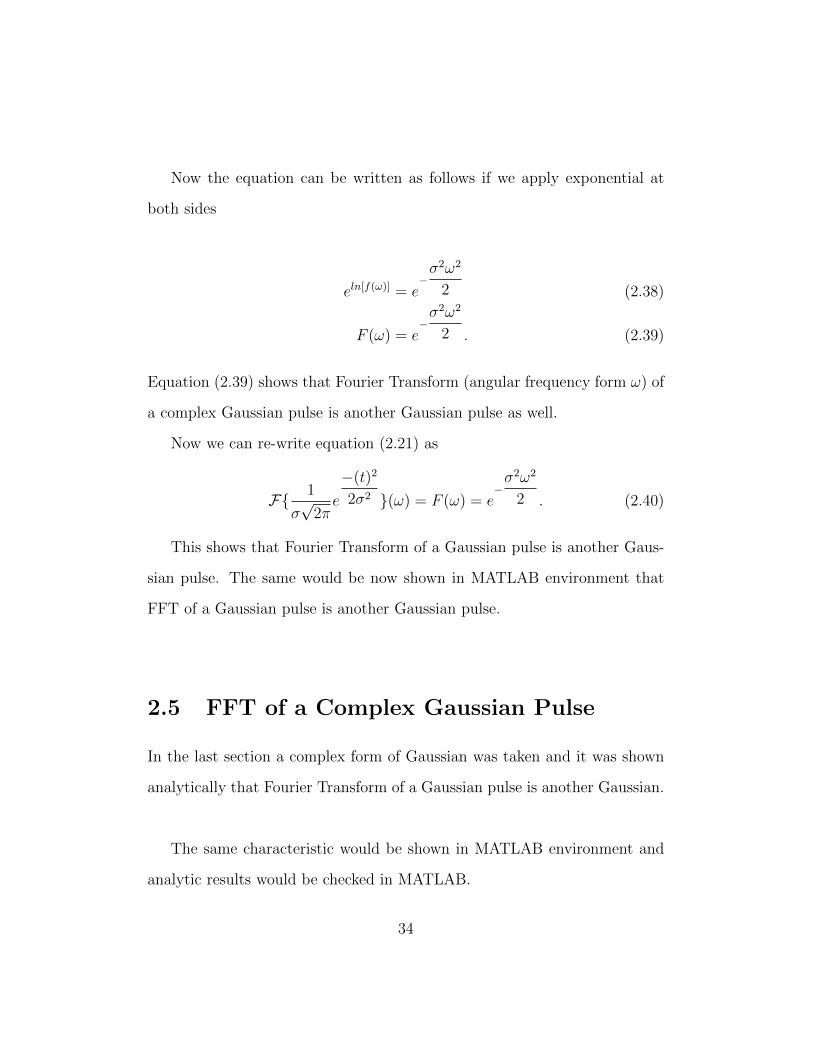
Consider the following Complex Form of Gaussian pulse from (2.19)
f(t) =1
σ√
2πe
−(t− µ)2
2σ2 . (2.41)
Figure 2.4: Complex Gaussian Pulse - temporal Form
For simplification purposes lets assume µ is taken zero where as σ = 1.
The time vector taken for Gaussian Pulse is −20s to 20s having N = 214
number of points.
The Gaussian pulse generated in figure in temporal form shows that its
mean is at zero as assumed in the equation with its variance being σ.
35
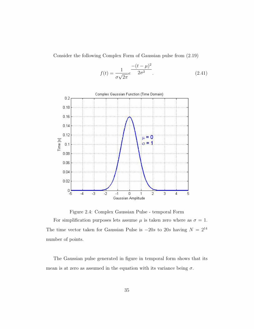
Figure 2.5: Complex Gaussian Pulse - spectral Form
FFT is applied on this complex Gaussian pulse and as it was shown in
last section that another Gaussian pulse in spectral form is generated. Figure
2.5 shows that analytic results are proven in MATLAB environment as well
that Fourier Transform of a Gaussian pulse is another Gaussian pulse.
36
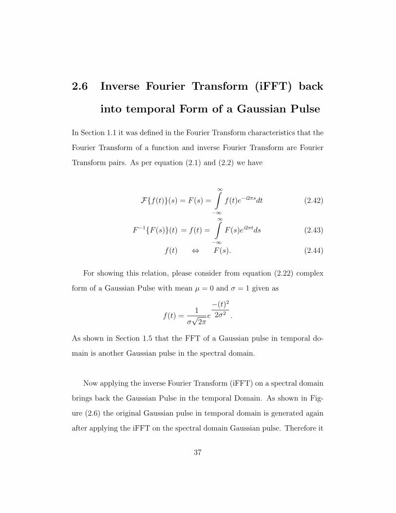
2.6 Inverse Fourier Transform (iFFT) back
into temporal Form of a Gaussian Pulse
In Section 1.1 it was defined in the Fourier Transform characteristics that the
Fourier Transform of a function and inverse Fourier Transform are Fourier
Transform pairs. As per equation (2.1) and (2.2) we have
F{f(t)}(s) = F (s) =
∞∫−∞
f(t)e−i2πsdt (2.42)
F−1{F (s)}(t) = f(t) =
∞∫−∞
F (s)ei2πtds (2.43)
f(t) ⇔ F (s). (2.44)
For showing this relation, please consider from equation (2.22) complex
form of a Gaussian Pulse with mean µ = 0 and σ = 1 given as
f(t) =1
σ√
2πe
−(t)2
2σ2 .
As shown in Section 1.5 that the FFT of a Gaussian pulse in temporal do-
main is another Gaussian pulse in the spectral domain.
Now applying the inverse Fourier Transform (iFFT) on a spectral domain
brings back the Gaussian Pulse in the temporal Domain. As shown in Fig-
ure (2.6) the original Gaussian pulse in temporal domain is generated again
after applying the iFFT on the spectral domain Gaussian pulse. Therefore it
37
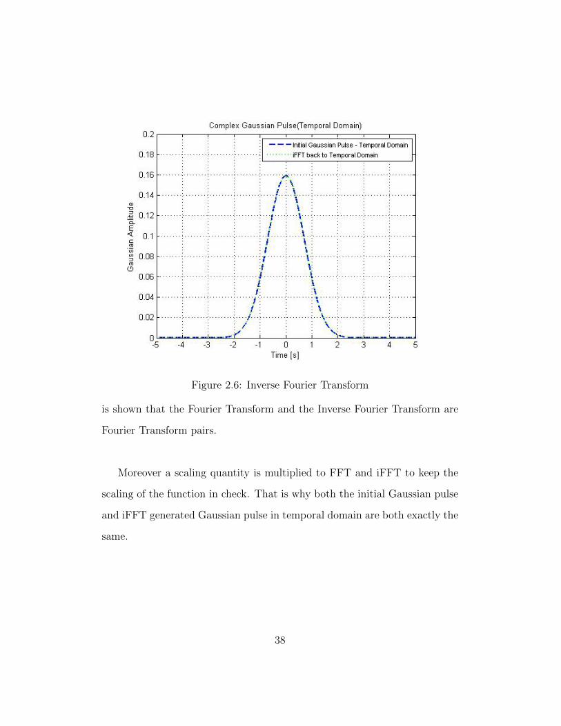
Figure 2.6: Inverse Fourier Transform
is shown that the Fourier Transform and the Inverse Fourier Transform are
Fourier Transform pairs.
Moreover a scaling quantity is multiplied to FFT and iFFT to keep the
scaling of the function in check. That is why both the initial Gaussian pulse
and iFFT generated Gaussian pulse in temporal domain are both exactly the
same.
38
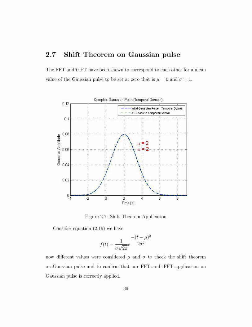
2.7 Shift Theorem on Gaussian pulse
The FFT and iFFT have been shown to correspond to each other for a mean
value of the Gaussian pulse to be set at zero that is µ = 0 and σ = 1.
Figure 2.7: Shift Theorem Application
Consider equation (2.19) we have
f(t) =1
σ√
2πe
−(t− µ)2
2σ2
now different values were considered µ and σ to check the shift theorem
on Gaussian pulse and to confirm that our FFT and iFFT application on
Gaussian pulse is correctly applied.
39
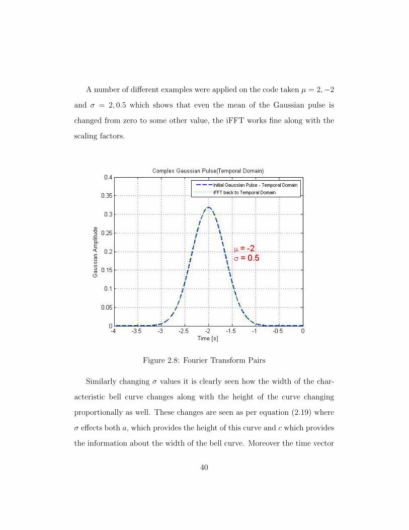
A number of different examples were applied on the code taken µ = 2,−2
and σ = 2, 0.5 which shows that even the mean of the Gaussian pulse is
changed from zero to some other value, the iFFT works fine along with the
scaling factors.
Figure 2.8: Fourier Transform Pairs
Similarly changing σ values it is clearly seen how the width of the char-
acteristic bell curve changes along with the height of the curve changing
proportionally as well. These changes are seen as per equation (2.19) where
σ effects both a, which provides the height of this curve and c which provides
the information about the width of the bell curve. Moreover the time vector
40
and frequency vector are kept same in all the examples i.e. time vector is
−20s to 20s having N = 214 number of points.
2.8 Time and Frequency Vector for FFT and
iFFT
The time vector and frequency vector for the FFT and iFFT are an impor-
tant part of Fourier Transform application in MATLAB. The time vector
and frequency vector are defined as such that give enough sampling points in
both temporal form and spectral form to generate a characteristic bell curve
for a Gaussian pulse.
The time vector for temporal domain chosen for FFT has tmin = −20
and tmax = 20. The time vector is set up
time = linspace(tmin, tmax,N)
where N = 214 Moreover a scaling factor dt is also calculated where dt =
2× tmaxN − 1
. The scaling factor dt is multiplied to the FFT for scaling purposes.
The Frequency vector chosen for spectral form is defined as
Freq = linspace(−fmax, fmax,N + 1)
where fmax =1
2× dt, and to have N number of points frequency vector is
again set as
Freq = Freq(1 : end− 1).
41
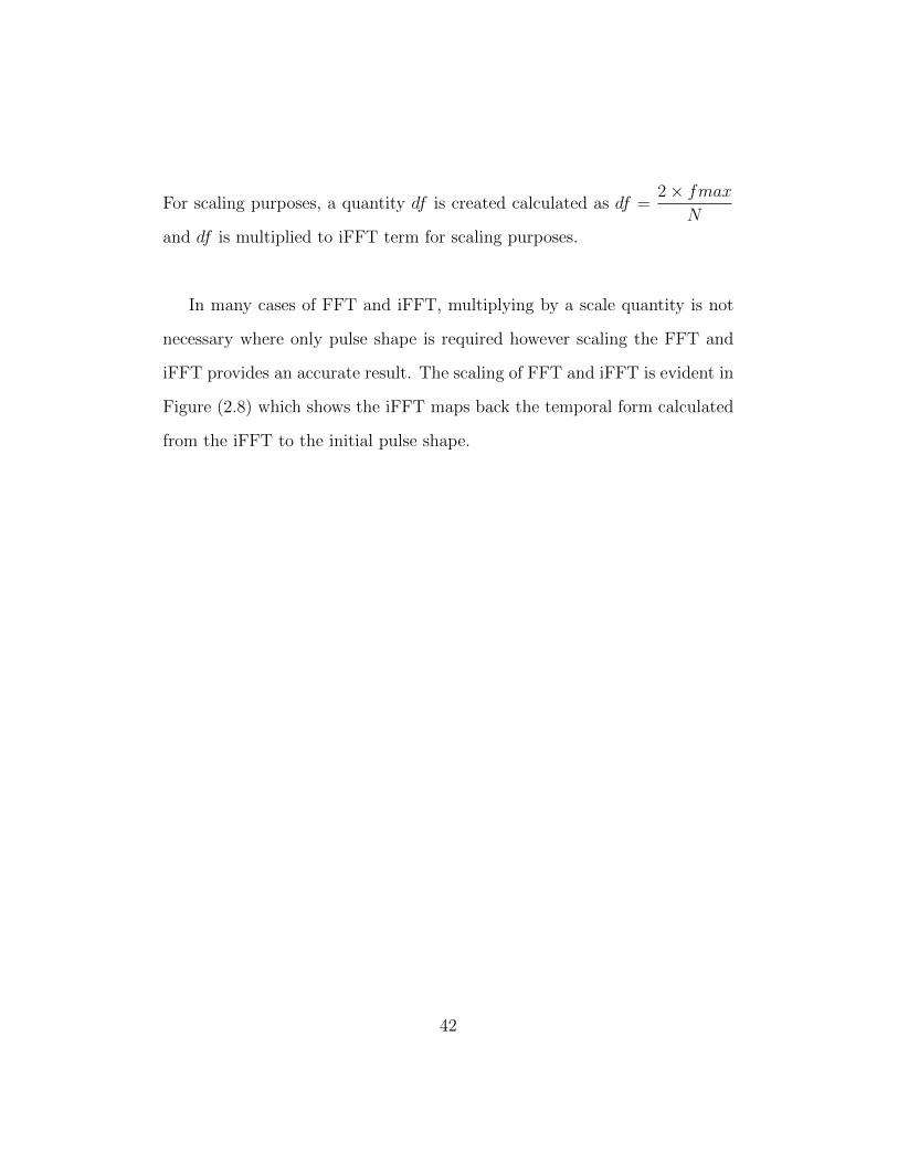
For scaling purposes, a quantity df is created calculated as df =2× fmax
Nand df is multiplied to iFFT term for scaling purposes.
In many cases of FFT and iFFT, multiplying by a scale quantity is not
necessary where only pulse shape is required however scaling the FFT and
iFFT provides an accurate result. The scaling of FFT and iFFT is evident in
Figure (2.8) which shows the iFFT maps back the temporal form calculated
from the iFFT to the initial pulse shape.
42
Chapter 3
Phase retrieval technique by
Using power Measurements
3.1 Phase retrieval technique
The proposed Phase retrieval technique is to establish a technique which
produces temporal phase and spectral phase using only measurements of
temporal power and spectral power.
It is assumed that actual temporal power measurements and spectral
power measurements of an optical signal are known however there is no in-
formation of the temporal and spectral phase measurements. A schematic
illustration of phase retrieval technique is shown in Figure 3.1
43
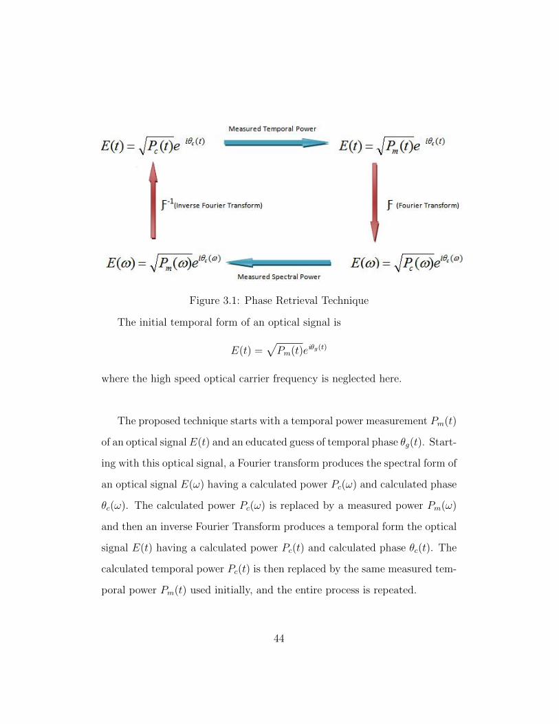
Figure 3.1: Phase Retrieval Technique
The initial temporal form of an optical signal is
E(t) =√Pm(t)eiθg(t)
where the high speed optical carrier frequency is neglected here.
The proposed technique starts with a temporal power measurement Pm(t)
of an optical signal E(t) and an educated guess of temporal phase θg(t). Start-
ing with this optical signal, a Fourier transform produces the spectral form of
an optical signal E(ω) having a calculated power Pc(ω) and calculated phase
θc(ω). The calculated power Pc(ω) is replaced by a measured power Pm(ω)
and then an inverse Fourier Transform produces a temporal form the optical
signal E(t) having a calculated power Pc(t) and calculated phase θc(t). The
calculated temporal power Pc(t) is then replaced by the same measured tem-
poral power Pm(t) used initially, and the entire process is repeated.
44
The calculated phases θc(t) and θc(ω) are updated each iteration while
the powers are substituted for their measured value as shown in Figure 3.1.
A number of iterations are to be performed until the phase or power values
converge.
3.2 Establishment of Phase Retrieval Tech-
nique
The phase phase retrieval technique is established in MATLAB environment.
Gaussian pulses are selected for the study of the phase retrieval technique
because of their unique behavior under the Fourier Transform and inverse
Fourier Transform.
3.2.1 Establishment of Actual Temporal and Spectral
Optical Signals
An optical signal consists of two parts, its optical power and its optical phase.
The form of the optical signal being used in the phase retrieval technique is
given as
E(t) =√P (t)eiθ(t) (3.1)
where P (t) is the optical signal power and eiθ(t) is the optical signal phase.
The phase retrieval technique is applied on a Gaussian pulse. An optical
signal in temporal form E(t) is created. The Initial temporal power measured
45
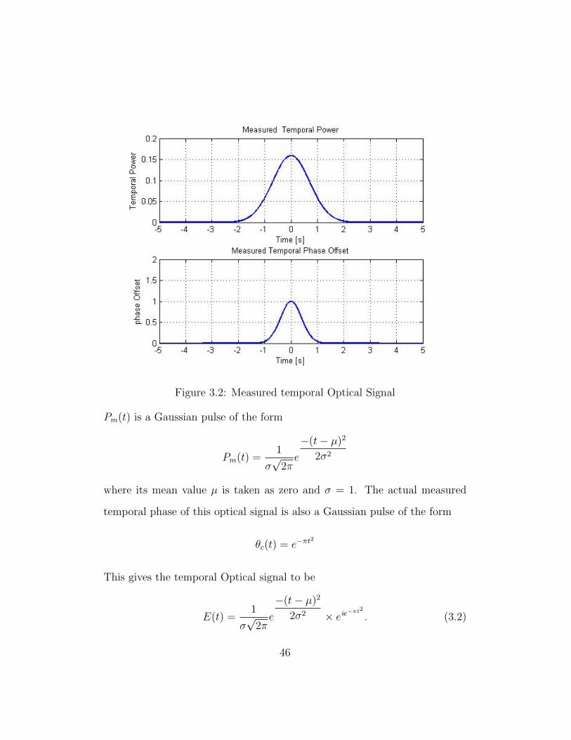
Figure 3.2: Measured temporal Optical Signal
Pm(t) is a Gaussian pulse of the form
Pm(t) =1
σ√
2πe
−(t− µ)2
2σ2
where its mean value µ is taken as zero and σ = 1. The actual measured
temporal phase of this optical signal is also a Gaussian pulse of the form
θc(t) = e−πt2
This gives the temporal Optical signal to be
E(t) =1
σ√
2πe
−(t− µ)2
2σ2 × eie−πt2
. (3.2)
46
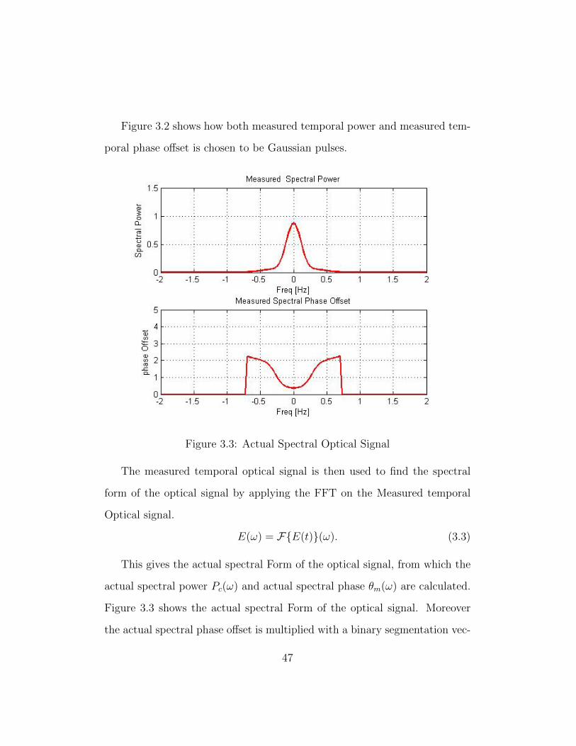
Figure 3.2 shows how both measured temporal power and measured tem-
poral phase offset is chosen to be Gaussian pulses.
Figure 3.3: Actual Spectral Optical Signal
The measured temporal optical signal is then used to find the spectral
form of the optical signal by applying the FFT on the Measured temporal
Optical signal.
E(ω) = F{E(t)}(ω). (3.3)
This gives the actual spectral Form of the optical signal, from which the
actual spectral power Pc(ω) and actual spectral phase θm(ω) are calculated.
Figure 3.3 shows the actual spectral Form of the optical signal. Moreover
the actual spectral phase offset is multiplied with a binary segmentation vec-
47
tor created by a low threshold value of the measured spectral power. This
shreds off the unwanted information created by computer noise and leaves of
the measured spectral phase offset which would be further explained in later
chapters.
Time and frequency vectors for temporal and spectral domains respec-
tively are created as discussed in the previous chapter. FFT and iFFT ap-
plied in the establishment of the phase retrieval technique are also scaled by
appropriate parameters as already discussed in the last chapter.
3.2.2 Establishment of Retrieval Algorithm having Mul-
tiple Iterations
The creation of measured temporal and spectral optical signals provides the
measured power spectrum of temporal Pm(t) and spectral Pm(ω) forms which
would be used in the retrieval algorithm as discussed in Section 4.1.
Now a guess temporal optical signal is created using the measured tem-
poral power Pm(t) and an educated guess of the temporal phase offset θg(t).
This educated phase offset is an educated guess of the form of a Gaussian
pulse different from the one used in the measured temporal phase offset.
The educated phase temporal optical signal is transformed into spectral
form by FFT using the scaling factor as discussed earlier. spectral optical
48
signal now consists of a calculated spectral power Pc(ω) and calculated spec-
tral phase θc(ω). The calculated spectral power is replaced by the measured
spectral power Pc(ω) as calculated in Section 3.2.1 and then an iFFT is ap-
plied on it to get a calculated temporal optical signal Ec(t) which consists of
calculated temporal power Pc(t) and calculated temporal phase θc(t). The
calculated temporal power is replaced by the measured temporal power Pm(t)
created in Section 3.2.1 and then FFT is applied on it to take it back into
the calculated spectral form.
The same process is repeated again to a certain number of iterations.
As we have created the measured optical signals therefore we can check the
calculated temporal phase values against the measured temporal phase values
and see if the retrieval algorithm actually converges the phase to its actual
known phase value.
49
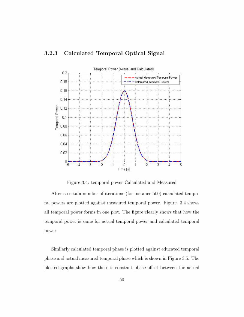
3.2.3 Calculated Temporal Optical Signal
Figure 3.4: temporal power Calculated and Measured
After a certain number of iterations (for instance 500) calculated tempo-
ral powers are plotted against measured temporal power. Figure 3.4 shows
all temporal power forms in one plot. The figure clearly shows that how the
temporal power is same for actual temporal power and calculated temporal
power.
Similarly calculated temporal phase is plotted against educated temporal
phase and actual measured temporal phase which is shown in Figure 3.5. The
plotted graphs show how there is constant phase offset between the actual
50
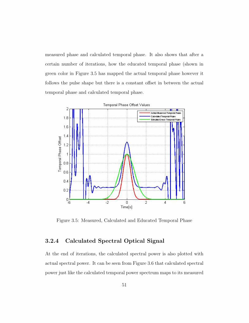
measured phase and calculated temporal phase. It also shows that after a
certain number of iterations, how the educated temporal phase (shown in
green color in Figure 3.5 has mapped the actual temporal phase however it
follows the pulse shape but there is a constant offset in between the actual
temporal phase and calculated temporal phase.
Figure 3.5: Measured, Calculated and Educated Temporal Phase
3.2.4 Calculated Spectral Optical Signal
At the end of iterations, the calculated spectral power is also plotted with
actual spectral power. It can be seen from Figure 3.6 that calculated spectral
power just like the calculated temporal power spectrum maps to its measured
51
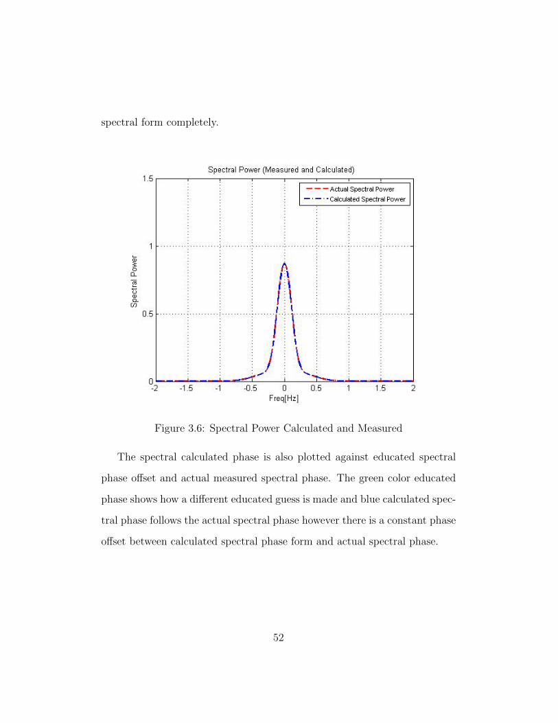
spectral form completely.
Figure 3.6: Spectral Power Calculated and Measured
The spectral calculated phase is also plotted against educated spectral
phase offset and actual measured spectral phase. The green color educated
phase shows how a different educated guess is made and blue calculated spec-
tral phase follows the actual spectral phase however there is a constant phase
offset between calculated spectral phase form and actual spectral phase.
52
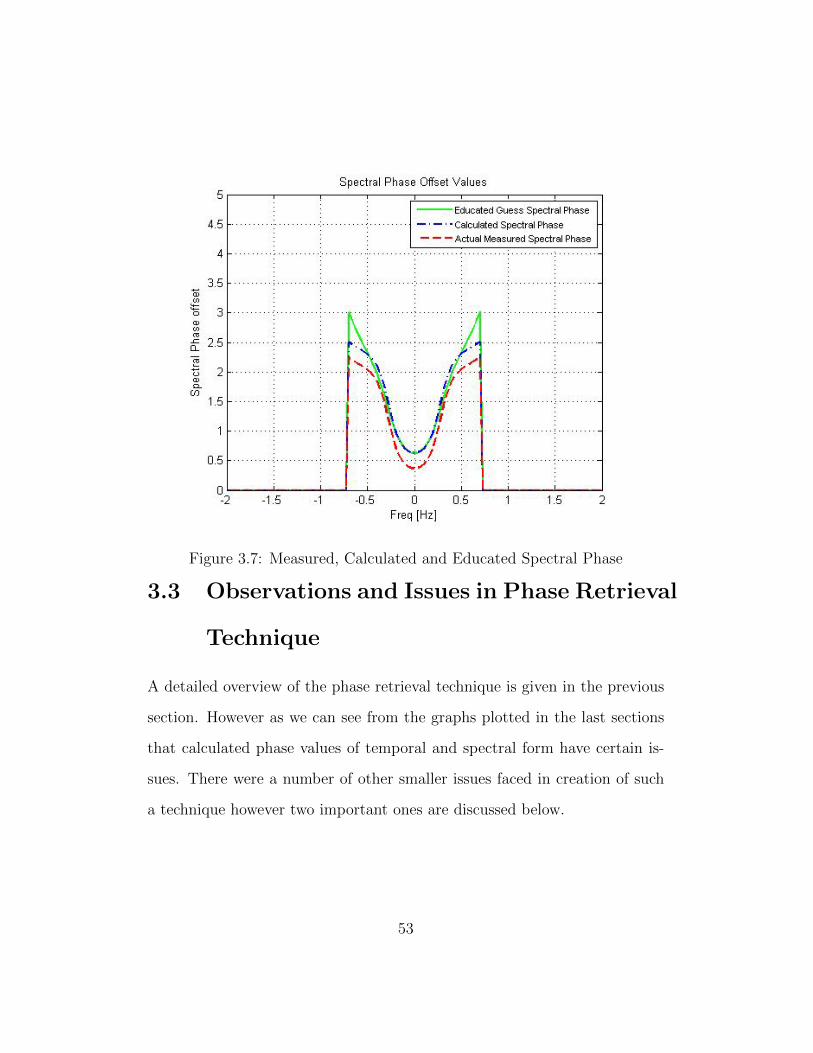
Figure 3.7: Measured, Calculated and Educated Spectral Phase
3.3 Observations and Issues in Phase Retrieval
Technique
A detailed overview of the phase retrieval technique is given in the previous
section. However as we can see from the graphs plotted in the last sections
that calculated phase values of temporal and spectral form have certain is-
sues. There were a number of other smaller issues faced in creation of such
a technique however two important ones are discussed below.
53
3.3.1 Constant Phase Offset
As it is seen in Figure 3.7 and Figure 3.5 there is a constant phase offset
between calculated temporal and spectral phase against their actual phase
forms. Similarly in temporal phase plotted graphs, there are a wings which
are created as we move farther from the mean value at each side.
The number of iterations was changed multiple times, giving different
number of iterations each time however it is found that their is a constant
phase offset between calculated temporal phase and actual temporal phase.
Similar constant phase offset is also observed in each case in spectral calcu-
lated phase and actual spectral phase.
3.3.2 Noise in Calculated Phase Forms
It is also further observed that there is some unwanted noise in the calculated
phase forms. In the temporal calculated phase there are creations of wings
which are seen as we move away from the mean of the Gaussian curve. These
wings are always there no matter how many iterations are run for retrieval
technique and each time gives rise to a different set of wings. These wings
can also be seen in Figure 3.5.
Similarly in spectral calculated phase, there are unwanted noise which
creates a difficulty in mapping out the required spectral phase values. As
54
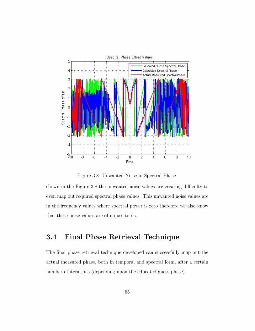
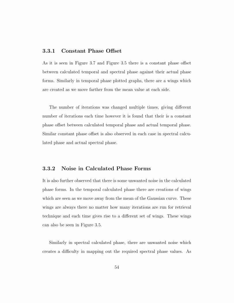
Figure 3.8: Unwanted Noise in Spectral Phase
shown in the Figure 3.8 the unwanted noise values are creating difficulty to
even map out required spectral phase values. This unwanted noise values are
in the frequency values where spectral power is zero therefore we also know
that these noise values are of no use to us.
3.4 Final Phase Retrieval Technique
The final phase retrieval technique developed can successfully map out the
actual measured phase, both in temporal and spectral form, after a certain
number of iterations (depending upon the educated guess phase).
55

Figure 3.9: Final Phase Retrieval Technique - Temporal Optical Signal
Figure 3.9 shows how the issues faced in constant phase offset is com-
pletely cleared. The calculated temporal power successfully maps the actual
temporal measured phase. Moreover there are no wings at the edges of
the calculated temporal phase as well. The techniques applied behind these
remedies would be discussed in later chapters.
56
Figure 3.10: Final Phase Retrieval Technique - Spectral Optical Signal
It can be seen how the spectral phase calculated maps successfully the
actual measured spectral phase and also there are no unwanted noise which
makes it easier to map out the required spectral phase values.
57
Chapter 4
Phase Retrieval Technique
Metrics
The phase retrieval technique using spectral and temporal power measure-
ments has been discussed in detail in last chapter. There were various prob-
lems which were faced during the development of the phase retrieval tech-
nique, some of which were discussed briefly in last chapter, however we were
able to overcome those issues and come up with a phase retrieval technique
which successfully maps out the actual phase. However, we believe, that dur-
ing the phase retrieval algorithm there should be a mechanism which tells us
the algorithms progress after each iteration (i.e. FFT into spectral form and
iFFT back into temporal form) and in a way informs us that whether we are
moving in the right direction or not.
An important part of the phase retrieval technique is to make an educated
58
guess about the required phase, and then applying the phase retrieval tech-
nique on the educated form of the optical signal. In order for us to observe
that whether our educated guess of the temporal phase was appropriately
chosen or not, we need to find a mechanism that informs us of our progress
in mapping out the actual temporal and spectral phase. That mechanism
will inform us that if we are getting closer to our main objective of retrieving
out the actual temporal and spectral phase information or if we are getting
even further away of our actual phase values.
This need for us to observe the progress of our phase retrieval algorithm
after each iteration lead us to use some algorithm progress metrics using cal-
culated power and phase measurements of spectral and temporal form. Each
metric defined in our algorithm will be explained below.
Metrics plotted below will be for the phase retrieval technique defined in
Section 3.4 where temporal power and phase measurements are shown in Fig-
ure 3.9 and spectral phase and power measurements are shown in Figure 3.10.
4.1 Power Metrics
We investigated different power metrics using both spectral power and tem-
poral power forms.
59
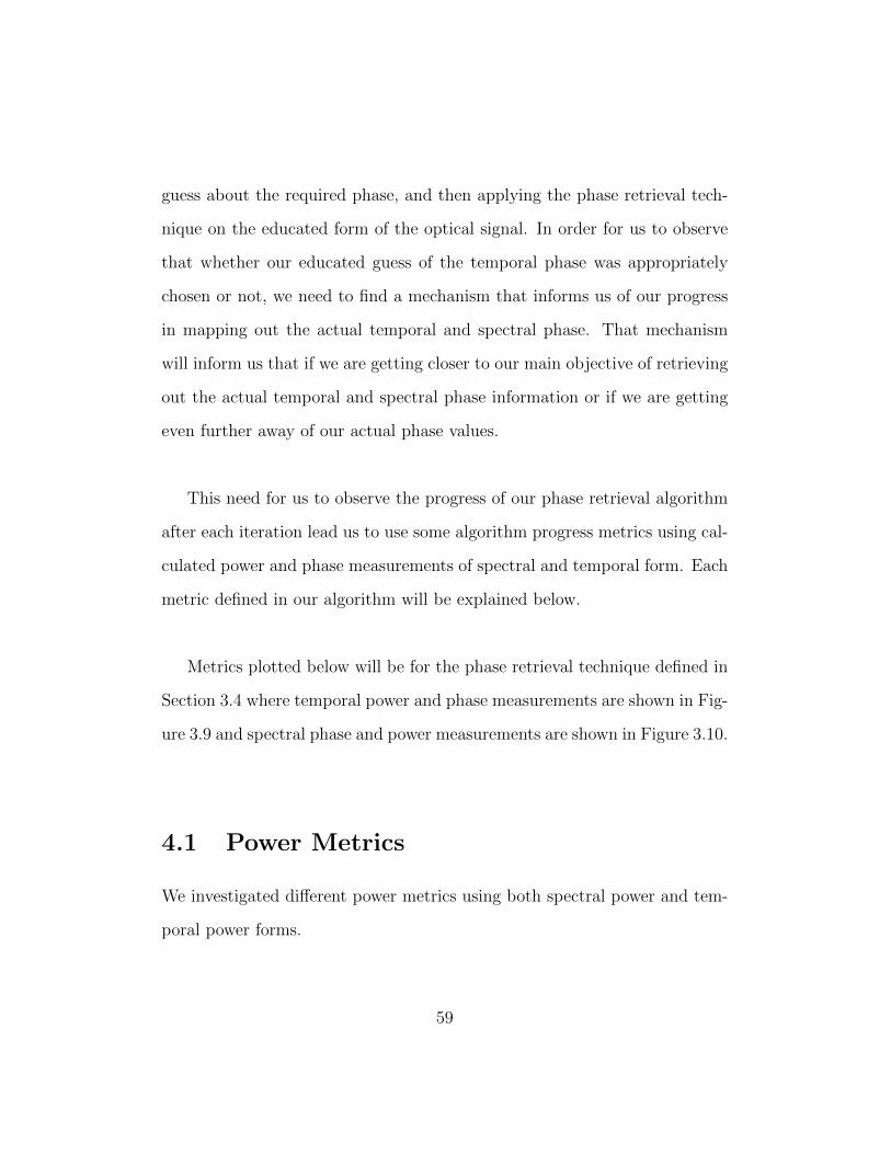
4.1.1 Temporal Power Metric
Figure 4.1: Temporal Power Metric Mtpow1
The temporal power metric is given by the following formula [8]
Mtpow1(n) =
√∑(Pc(t)− Pm(t))2∑
Pm(t). (4.1)
where Pc(t) is temporal power calculated vector after nth iteration and Pm(t)
is actual temporal power vector and n is nth number of iteration. At each
iteration this value is calculated.
This power metric is just taking a sum of the squared difference of the
calculated temporal power vector Pc(t) and measured temporal power vector
60

Pm(t) and dividing it by the sum of actual measured temporal power vector.
Taking a square of the difference of calculated temporal power and measured
temporal power gets rid of the negative sign.
This temporal power metric is calculated after each iteration and it is
plotted against the number of iterations showing a progress of phase retrieval
algorithm in calculated temporal power. If the temporal power metric is
getting closer to zero that suggests that the educated guess is rightly chosen
and calculated temporal power is mapping the actual actual temporal power
in the start. The same is shown in Figure 4.1 where temporal power metric
Mtpow1 is continuously decreasing till 200 iterations after which the change
is negligible. This also shows that 200 iterations are probably enough for
phase retrieval algorithm to map out the actual phase in temporal or spectral
form.
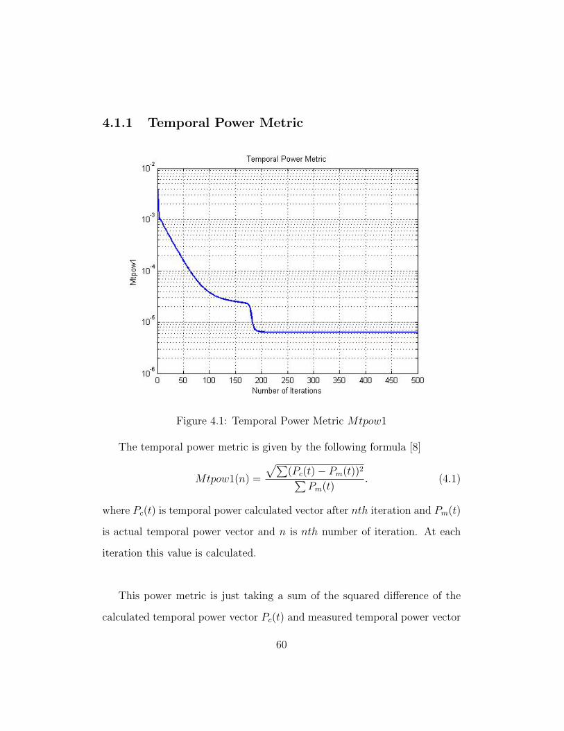
4.1.2 Spectral Power Metric
The spectral power metric mspow1 is given as
Mspow1(n) =
√∑(Pc(ω)− Pm(ω))2∑
Pm(ω). (4.2)
where we have Pc(ω) as spectral power calculated vector for nth iteration,
Pm(ω) as spectral power measured vector. Similarly n defines the nth itera-
tion.
The power metric for spectral power also finds a difference between the
61
Figure 4.2: Power Metrics Mtpow1 and Mspow1
calculated spectral power vector of each iteration and actual measured spec-
tral power. The difference is squared to get rid of any negative signs in the
process. The sum of differences is then divided by the sum of actual spectral
power vector.
The spectral power metric is plotted for each iterations and shows the
progress of phase retrieval technique in spectral power form. As we can see
from Figure 4.2 that the spectral power metric is decreasing showing posi-
tive progress towards mapping out the actual spectral power, which in return
would likely mean that the calculated spectral phase would be similarly map-
62
ping actual spectral phase.The total number of iterations are kept at 500 just
to show that a certain number of iterations are enough for mapping out the
phase as we can see in Figure 4.2 that 200 iterations are probably enough for
convergence of temporal and spectral power.
4.2 Phase Metrics
To check progress of calculated phase of optical signal, phase metrics are also
developed.
4.2.1 Temporal Phase Metric
There are two temporal phase metrics developed for the phase retrieval tech-
nique.
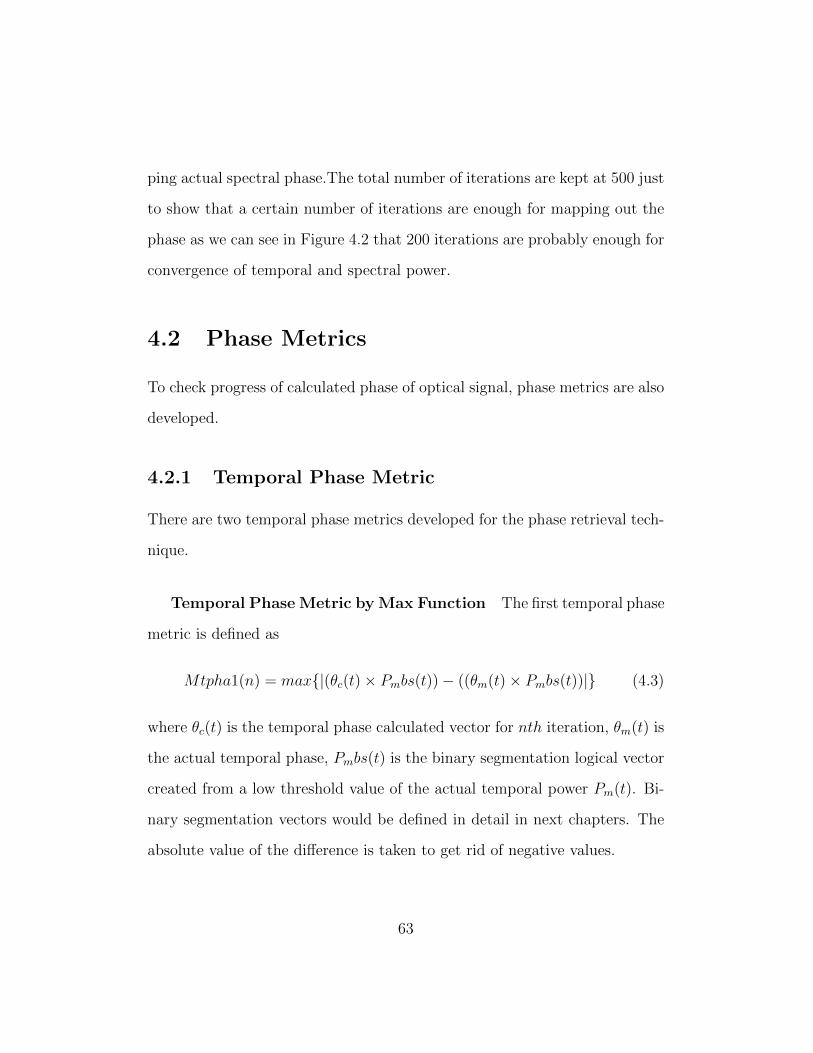
Temporal Phase Metric by Max Function The first temporal phase
metric is defined as
Mtpha1(n) = max{|(θc(t)× Pmbs(t))− ((θm(t)× Pmbs(t))|} (4.3)
where θc(t) is the temporal phase calculated vector for nth iteration, θm(t) is
the actual temporal phase, Pmbs(t) is the binary segmentation logical vector
created from a low threshold value of the actual temporal power Pm(t). Bi-
nary segmentation vectors would be defined in detail in next chapters. The
absolute value of the difference is taken to get rid of negative values.
63
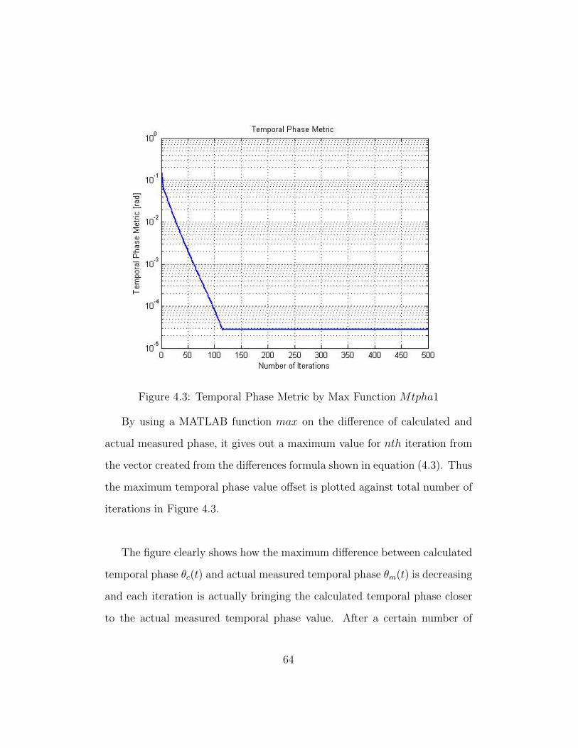
Figure 4.3: Temporal Phase Metric by Max Function Mtpha1
By using a MATLAB function max on the difference of calculated and
actual measured phase, it gives out a maximum value for nth iteration from
the vector created from the differences formula shown in equation (4.3). Thus
the maximum temporal phase value offset is plotted against total number of
iterations in Figure 4.3.
The figure clearly shows how the maximum difference between calculated
temporal phase θc(t) and actual measured temporal phase θm(t) is decreasing
and each iteration is actually bringing the calculated temporal phase closer
to the actual measured temporal phase value. After a certain number of
64
iterations the difference becomes closer to zero.
Figure 4.4: Temporal Phase Metrics Mtpha1 and Mtpha2
Temporal Phase Metric by Summation of differences Formula
The second temporal phase metric Mtpha2 uses a summations of differences
formula which is given by
Mtpha2(n) =
√∑([θc(t)× Pmbs(t)]− [θm(t)× Pmbs(t)])2∑
(θm(t)× Pmbs(t)). (4.4)
where θc(t) is the temporal phase calculated vector for nth iteration, θm(t)
is the actual temporal phase, Pmbs(t) is the binary segmentation logical vec-
tor created from a low threshold value of the actual temporal power Pm(t).
65
This temporal phase metric is created in the same way as the power
metrics. This temporal phase metric doesn’t point out any one point in the
calculated phase but makes a vector of the differences of the actual temporal
phase θm(t) and calculated temporal phase θc(t). The plotted Figure 4.4
clearly shows how the difference values is decreasing with increase in the
number of iterations and each iteration is making the calculated temporal
phase more closer to the actual temporal measured phase value. This metric
shows more detail than the temporal phase metric created with just the
max function as it takes into effect minute changes in the whole calculated
temporal phase. The binary segmentation vector helps in shredding off the
unwanted noise in the calculated temporal phase.
4.2.2 Spectral Phase Metric
There are two spectral phase metrics created.
Spectral Phase Metric by Max Function The spectral phase dif-
ference metric is given by
Mspha1(n) = max{|(θc(ω)× Pmbs(ω))− ((θm(ω)× Pmbs(ω))|}. (4.5)
where θc(ω) is the spectral phase calculated vector for nth iteration, θm(ω)
is the actual spectral phase, Pmbs(ω) is the binary segmentation logical vec-
tor created from a low threshold value of the actual spectral power vector
Pm(ω). The binary segmentation vector is used to shred off the unwanted
noise in phase vector.
66
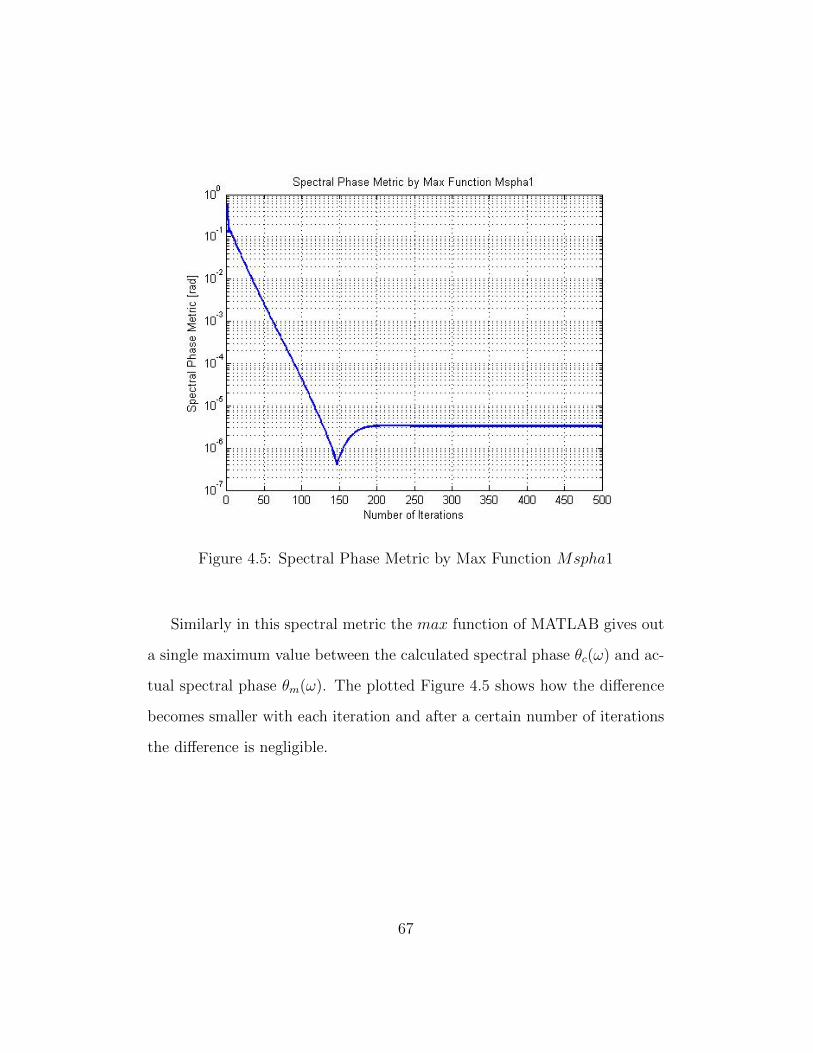
Figure 4.5: Spectral Phase Metric by Max Function Mspha1
Similarly in this spectral metric the max function of MATLAB gives out
a single maximum value between the calculated spectral phase θc(ω) and ac-
tual spectral phase θm(ω). The plotted Figure 4.5 shows how the difference
becomes smaller with each iteration and after a certain number of iterations
the difference is negligible.
67
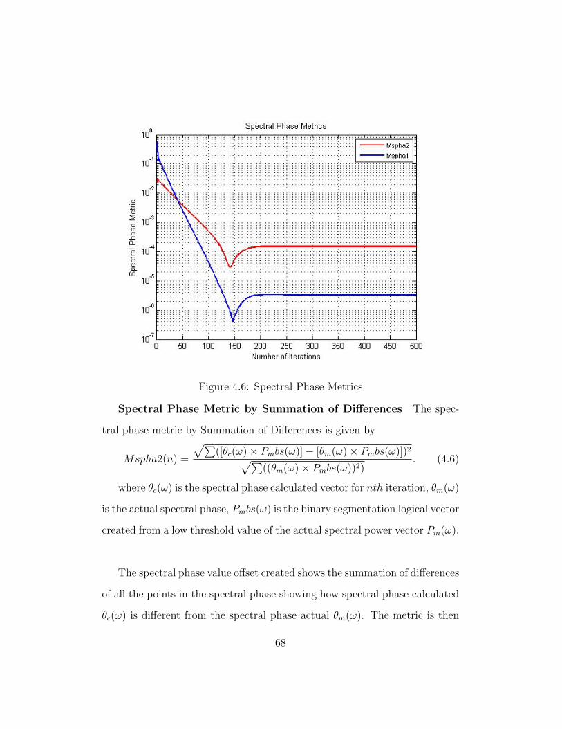
Figure 4.6: Spectral Phase Metrics
Spectral Phase Metric by Summation of Differences The spec-
tral phase metric by Summation of Differences is given by
Mspha2(n) =
√∑([θc(ω)× Pmbs(ω)]− [θm(ω)× Pmbs(ω)])2√∑
((θm(ω)× Pmbs(ω))2). (4.6)
where θc(ω) is the spectral phase calculated vector for nth iteration, θm(ω)
is the actual spectral phase, Pmbs(ω) is the binary segmentation logical vector
created from a low threshold value of the actual spectral power vector Pm(ω).
The spectral phase value offset created shows the summation of differences
of all the points in the spectral phase showing how spectral phase calculated
θc(ω) is different from the spectral phase actual θm(ω). The metric is then
68
plotted against each iteration showing clearly if there is an increase in the
difference or decrease in the difference. If we observe Figure 4.6 we can see
that how the spectral phase offset is decreasing continuously however it also
shows a dip at 150 iteration after which it settles down closer to the actual
spectral phase.
The Figure 4.6 shows how if there are some unique issues in our algorithm,
any unusual dips or spikes, we can observe them by using these metrics. By
using metrics in each temporal and spectral form and following spectral and
temporal power and phase values progress in each iteration we are able to
observe minute changes in our algorithm.
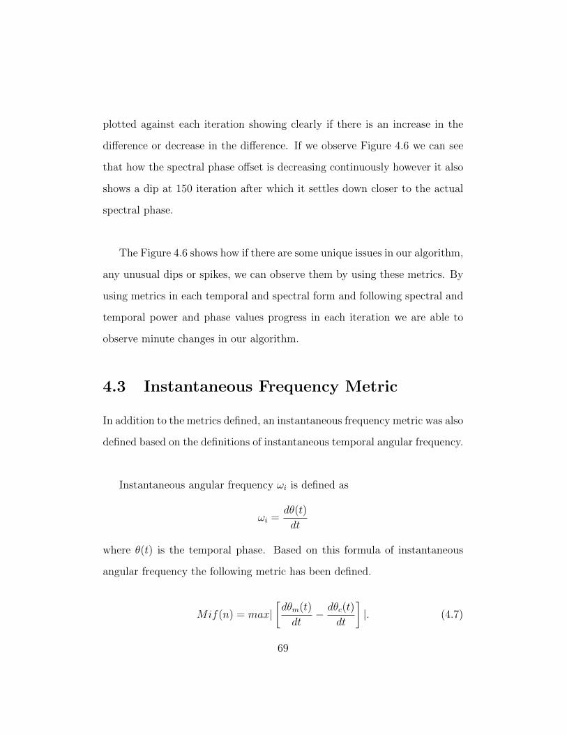
4.3 Instantaneous Frequency Metric
In addition to the metrics defined, an instantaneous frequency metric was also
defined based on the definitions of instantaneous temporal angular frequency.
Instantaneous angular frequency ωi is defined as
ωi =dθ(t)
dt
where θ(t) is the temporal phase. Based on this formula of instantaneous
angular frequency the following metric has been defined.
Mif(n) = max|[dθm(t)
dt− dθc(t)
dt
]|. (4.7)
69
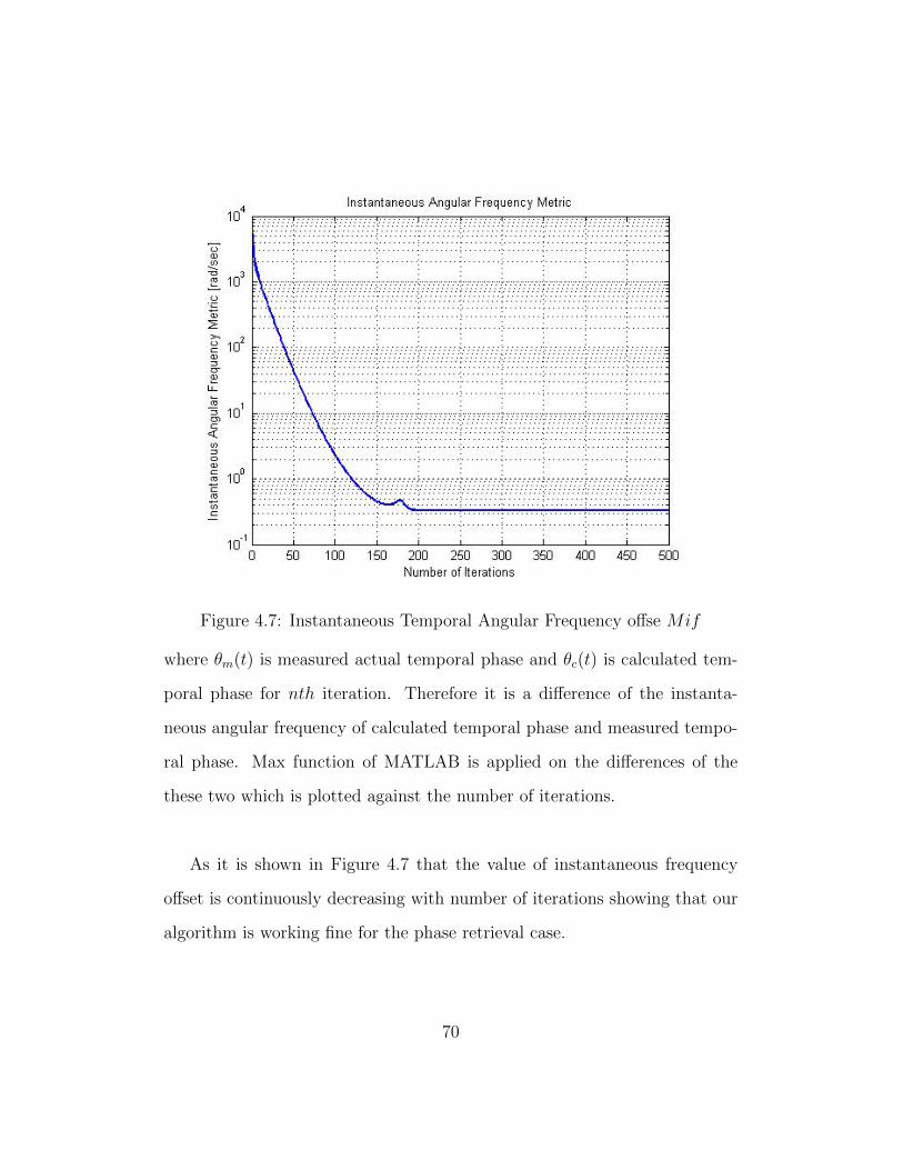
Figure 4.7: Instantaneous Temporal Angular Frequency offse Mif
where θm(t) is measured actual temporal phase and θc(t) is calculated tem-
poral phase for nth iteration. Therefore it is a difference of the instanta-
neous angular frequency of calculated temporal phase and measured tempo-
ral phase. Max function of MATLAB is applied on the differences of the
these two which is plotted against the number of iterations.
As it is shown in Figure 4.7 that the value of instantaneous frequency
offset is continuously decreasing with number of iterations showing that our
algorithm is working fine for the phase retrieval case.
70
In many cases of phase retrieval processes, the pulse shape is required
and hence such a metric defined accordingly with the change in phase value
with change in time. Alongside this metric, we have also plotted instanta-
neous angular frequency of calculated temporal phase and measured actual
temporal phase and is shown in Figure 4.8.
Figure 4.8: Instantaneous Temporal Angular Frequency (nth iteration)
Figure 4.8 is showing instantaneous angular frequencydθ(t)
dtof tempo-
ral measured and calculated phase values over each other showing how the
change in phase with time is the same for both calculated and measured
forms of temporal phase for nth iteration. Any iteration can be chosen in
the algorithm and can be plotted for as required and Figure 4.8 is the plot
71
for n = 500.
4.4 Metrics Summary
A number of different metrics were developed using phase and power values
at different stages of the phase retrieval algorithm. All these metrics can be
used in various techniques. Bu developing metrics which follow algorithms
progress in both spectral form and temporal form has allowed us to use dif-
ferent metrics for different techniques. For instance, in some examples the
change in the temporal phase or spectral phase might not be enough to de-
duce any satisfactory results however the same change in temporal power
metric might be observed in unusual spikes. One such example was using
chirp phases signals in the algorithm which would be discussed in later chap-
ters.
Therefore all of these metrics are developed keeping in mind that different
metric can be used in different circumstances.
72
Chapter 5
Constant Phase Offset in Phase
Retrieval Technique
It was discussed briefly in Chapter 3 that the phase retrieval technique al-
ways gave a constant phase offset in its final calculated temporal and spectral
phase. As shown in Figure 5.1 and 5.2 both the spectral and temporal calcu-
lated phase are having an offset from the actual spectral and temporal phase
respectively. This issue was observed constantly even if we keep on running
the iterations.
In addition to the constant offset, there is an unwanted noise for both
spectral and temporal phase as we move away from the mean value of µ = 0.
As we can also observe from Figure 5.1 and Figure 5.2 that in both cases of
temporal and spectral phase, the unwanted noise functions which are present
are in the areas where temporal power and spectral power are zero.
73
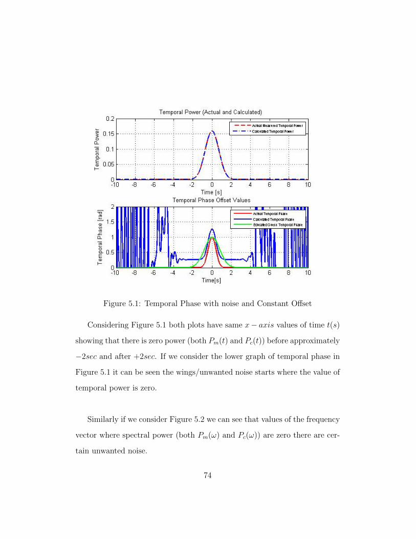
Figure 5.1: Temporal Phase with noise and Constant Offset
Considering Figure 5.1 both plots have same x− axis values of time t(s)
showing that there is zero power (both Pm(t) and Pc(t)) before approximately
−2sec and after +2sec. If we consider the lower graph of temporal phase in
Figure 5.1 it can be seen the wings/unwanted noise starts where the value of
temporal power is zero.
Similarly if we consider Figure 5.2 we can see that values of the frequency
vector where spectral power (both Pm(ω) and Pc(ω)) are zero there are cer-
tain unwanted noise.
74
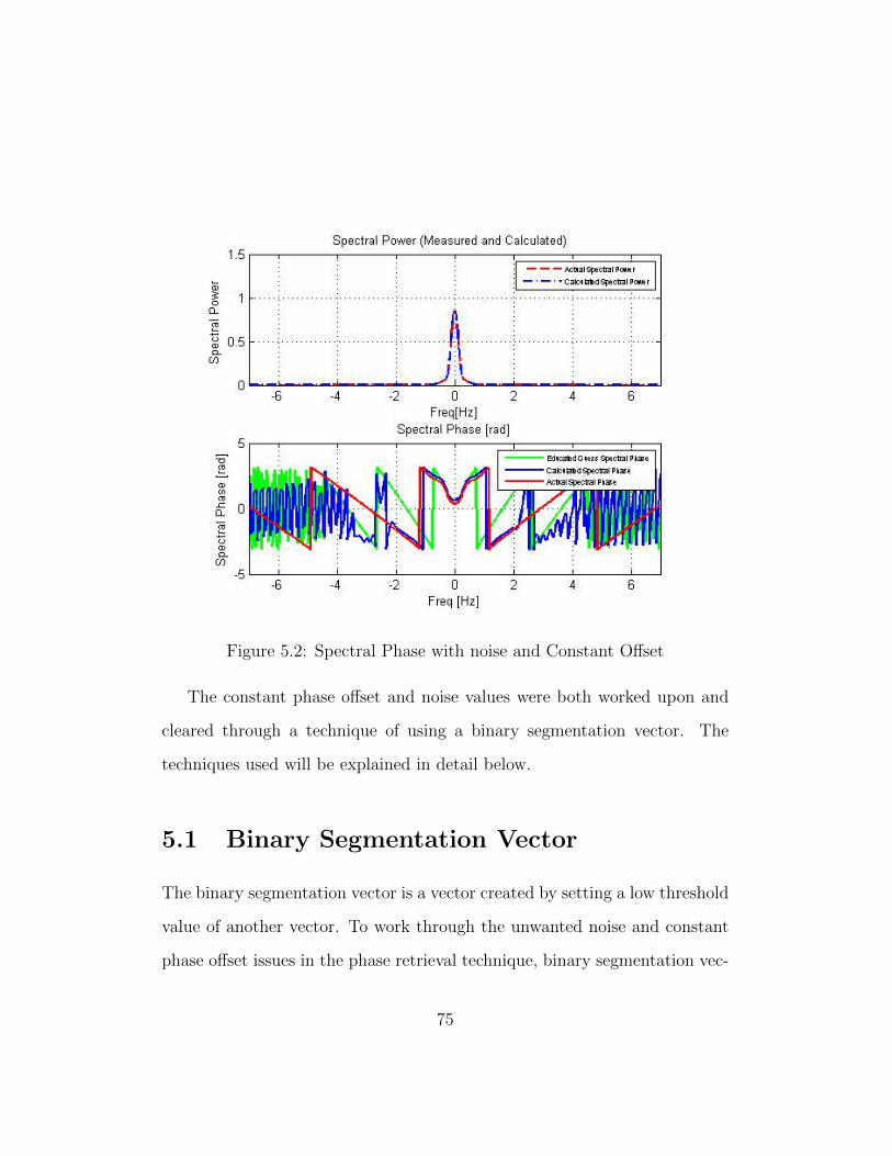
Figure 5.2: Spectral Phase with noise and Constant Offset
The constant phase offset and noise values were both worked upon and
cleared through a technique of using a binary segmentation vector. The
techniques used will be explained in detail below.
5.1 Binary Segmentation Vector
The binary segmentation vector is a vector created by setting a low threshold
value of another vector. To work through the unwanted noise and constant
phase offset issues in the phase retrieval technique, binary segmentation vec-
75
tors were created.
5.1.1 Temporal Power Binary Segmentation Vector
Figure 5.3: Temporal Phase with Binary segmenatation vector threshold =
0.001
A temporal power binary segmentation vector Pmbs(t) was created by
setting up a low threshold value of actual temporal power given as
Pmbs(t) = Pm(t) > threshold
where threshold is a low value set up accordingly. This results in creation of
a binary segmentation vector which has a binary value of 1 at all the points
76
greater than threshold value and a binary value of 0 at all the points which
are less than threshold.
The resultant temporal power binary segmentation vector when multi-
plied with calculated temporal phase results in getting rid off all the phase
values other than where the Power is more than the threshold value. In this
way we get rid off the phase information which we don’t care about and keep
the phase information which is important to us.
Considering Figure 5.1 and multiplying calculated temporal phase with
the temporal power binary segmentation vector we get Figure 5.3 which
shows how the unwanted wings/noise is no more to be observed.
5.1.2 Spectral Power Binary Segmentation Vector
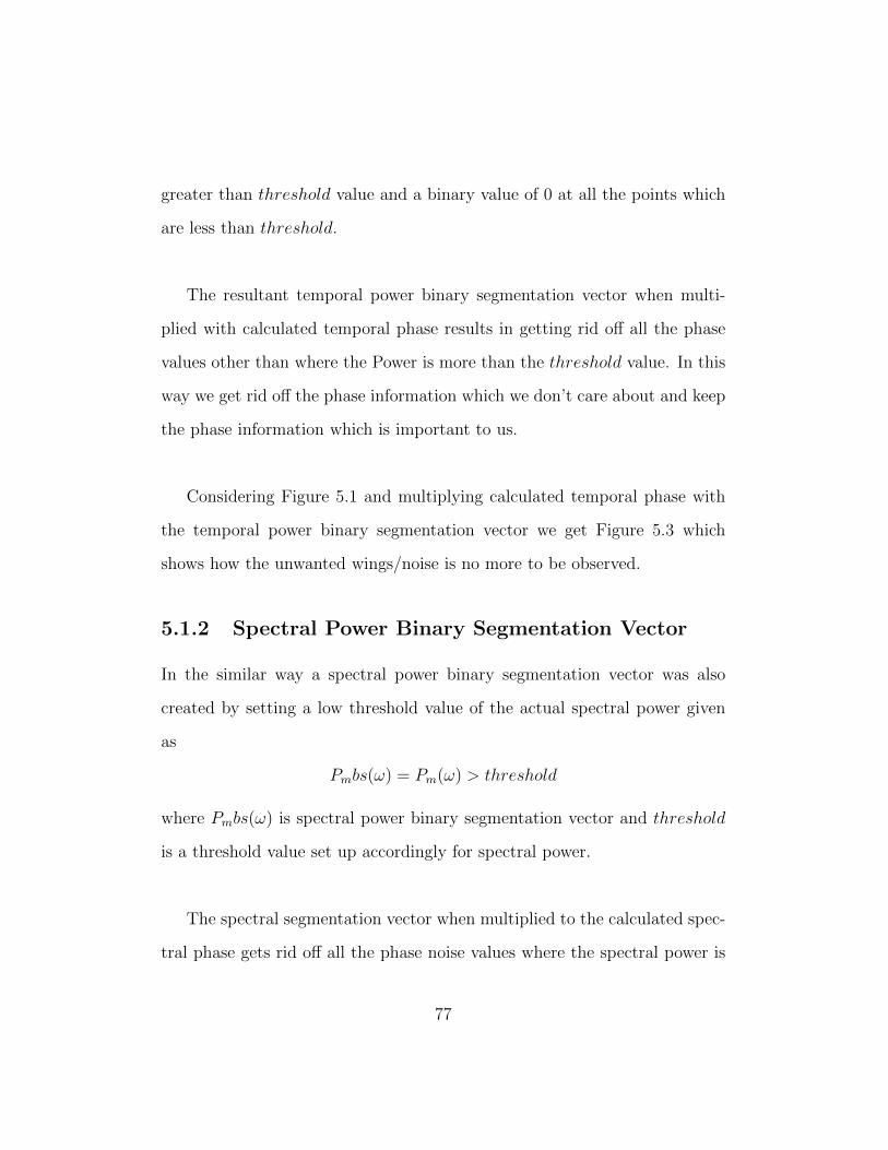
In the similar way a spectral power binary segmentation vector was also
created by setting a low threshold value of the actual spectral power given
as
Pmbs(ω) = Pm(ω) > threshold
where Pmbs(ω) is spectral power binary segmentation vector and threshold
is a threshold value set up accordingly for spectral power.
The spectral segmentation vector when multiplied to the calculated spec-
tral phase gets rid off all the phase noise values where the spectral power is
77
less than the threshold value. Considering Figure 5.2 if we set up a spectral
power binary segmentation vector we get rid of all the noise phase and thus
we can just get the required results of phase as shown in Figure 5.4.
Figure 5.4: Spectral Phase with Binary segmenatation vector threshold =
0.008
Figure 5.4 and 5.3 show that we can get rid of noise by using binary
segmentation vectors in our plots.
78
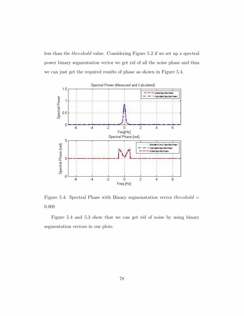
5.2 Constant Phase Offset Removal Technique
As it is observed in 5.1 that there is a constant phase offset which is there in
the temporal phase. However by use of the binary segmentation vector with
in our phase retrieval technique, we can get rid of this constant phase offset.
Figure 5.5: Temporal and Spectral Phase without Phase Offset threshold =
0.02
The technique defined for removal of a constant offset includes setting up
a low threshold value of the temporal power and creating a temporal power
binary segmentation vector in the start of the phase retrieval technique as
79
follows
Pmbs(t) = Pm(t) > threshold.
In the next step, to get rid of unwanted temporal phase information calcu-
lated temporal phase θc(t) is fine tuned as
θc(t)(n) = θc(t)(n).× Pmbs(t)
where n stands for nth iteration. By multiplying binary segmentation vector
Pmbs(t) with calculated temporal phase θc(t) in nth iteration, calculated tem-
poral phase is fine tuned and all unwanted phase/noise values are nullified.
This means that in ever nth iteration the unwanted noise values are nullified
in calculated temporal phase and the same noise values are not taken into
account again in nth+ 1 iteration.
Applying such technique removes the constant phase offset in both tem-
poral and spectral calculated phases. Considering phase plots in Figure 5.2
and 5.1, by applying this technique constant phase offset can be removed as
shown in Figure 5.5 where temporal phase calculated in every iteration is
fine tuned by a binary segmentation vector defined above.
Moreover a number of test cases were taken and total number of itera-
tions were increased as far as 4000 just to check that if the same technique
doesn’t give any unusual behavior once the calculated temporal phase maps
the actual temporal phase but no abnormality was found. It was observed
that a few number of iterations ranging from 50 to 200, depending upon the
80

educated guess phase, were required for phase retrieval with this technique.
Any more number of iterations just keeps the retrieved phase the same, which
was confirmed by the phase metrics defined in last chapter.
81
Chapter 6
Impact of Educated Guess
Phase on Phase Retrieval
Technique
The phase retrieval technique has been shown to achieve successfully the ac-
tual temporal and spectral phases after an improvised technique of binary
segmentation. However in previous chapters phase retrieval technique was
applied with only one educated guess of temporal phase. In this chapter dif-
ferent educated guesses of temporal phase would be tested against the phase
retrieval algorithm to check how it responds.
In all the cases that would be discussed in this chapter, the actual tem-
poral optical signal and spectral signal would be kept constant. However
different educated temporal phase guesses will be applied to check the phase
82
retrieval algorithm response. Figure 6.1 shows the actual temporal and spec-
tral power and phase.
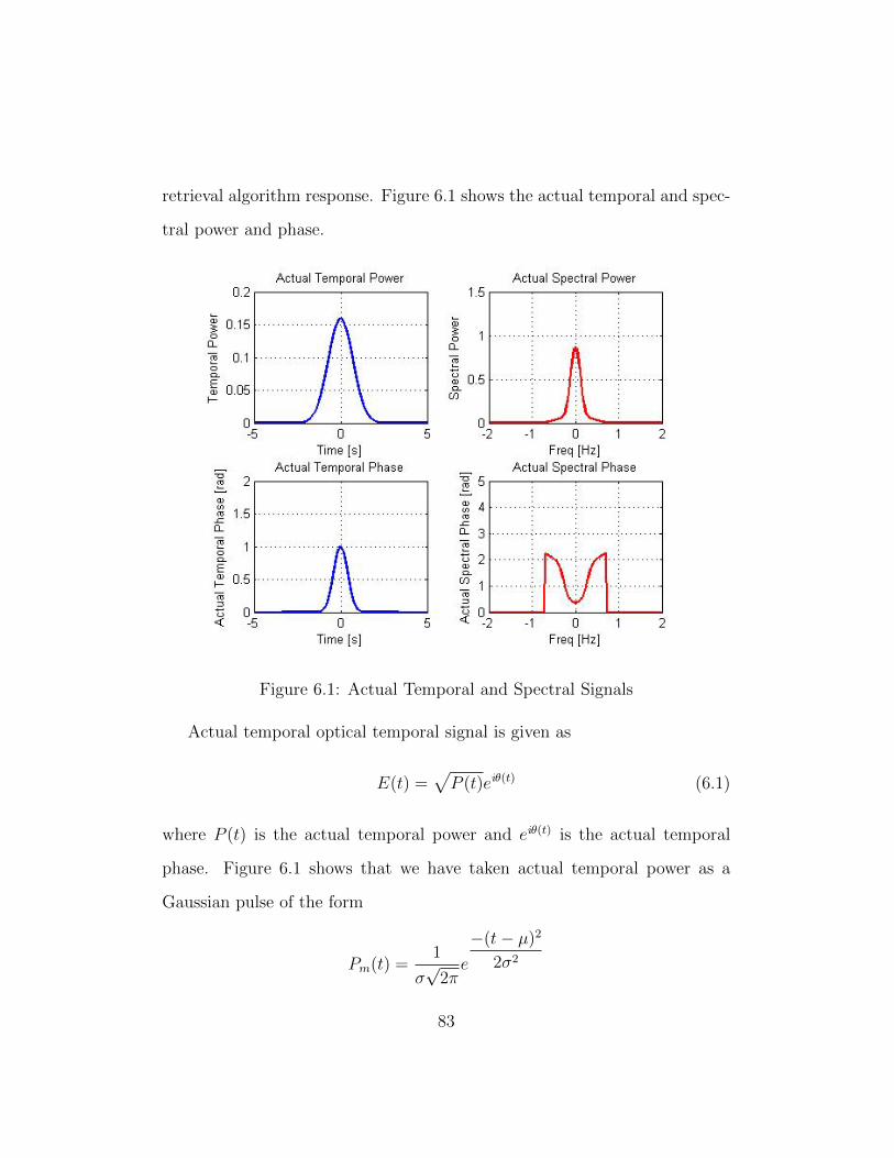
Figure 6.1: Actual Temporal and Spectral Signals
Actual temporal optical temporal signal is given as
E(t) =√P (t)eiθ(t) (6.1)
where P (t) is the actual temporal power and eiθ(t) is the actual temporal
phase. Figure 6.1 shows that we have taken actual temporal power as a
Gaussian pulse of the form
Pm(t) =1
σ√
2πe
−(t− µ)2
2σ2
83
where its mean value µ is taken as zero and σ = 1. The actual measured
temporal phase of this optical signal is also a Gaussian pulse of the form
θa(t) = e−πt2
.
The FFT of actual temporal optical signal gives us the actual spectral
power and phase as shown in Figure 6.1.
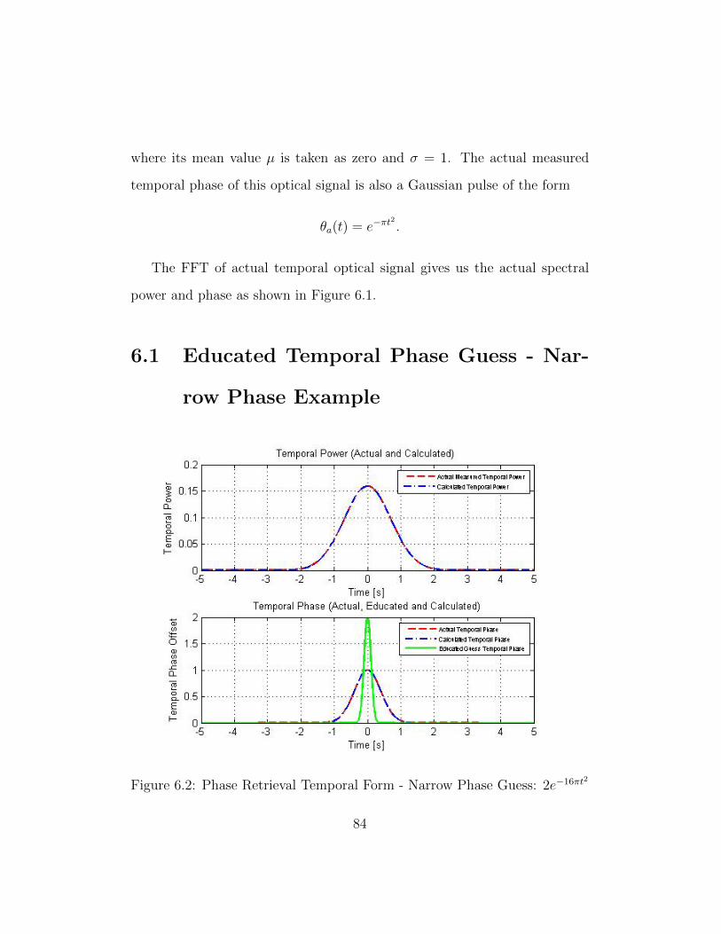
6.1 Educated Temporal Phase Guess - Nar-
row Phase Example
Figure 6.2: Phase Retrieval Temporal Form - Narrow Phase Guess: 2e−16πt2
84
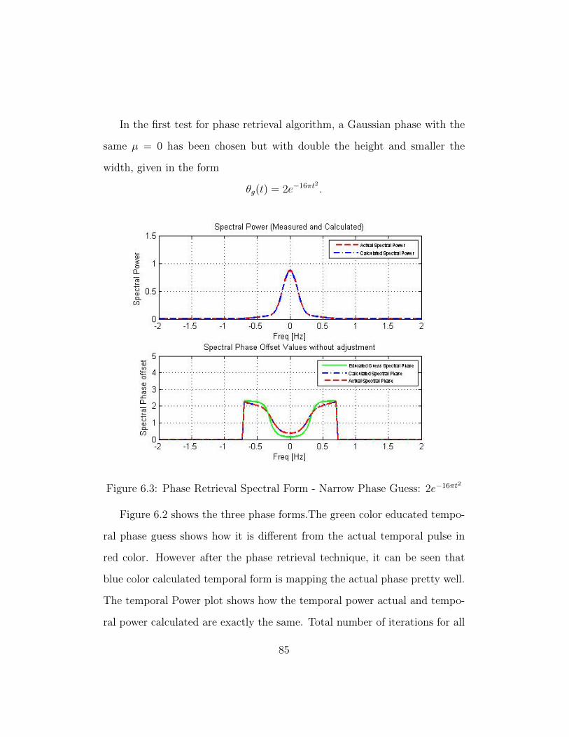
In the first test for phase retrieval algorithm, a Gaussian phase with the
same µ = 0 has been chosen but with double the height and smaller the
width, given in the form
θg(t) = 2e−16πt2
.
Figure 6.3: Phase Retrieval Spectral Form - Narrow Phase Guess: 2e−16πt2
Figure 6.2 shows the three phase forms.The green color educated tempo-
ral phase guess shows how it is different from the actual temporal pulse in
red color. However after the phase retrieval technique, it can be seen that
blue color calculated temporal form is mapping the actual phase pretty well.
The temporal Power plot shows how the temporal power actual and tempo-
ral power calculated are exactly the same. Total number of iterations for all
85
convergence plots in this chapter is N = 500 which would be shown in metric
plots how the convergence takes place as a function of N .
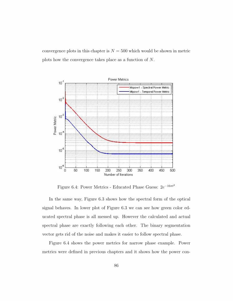
Figure 6.4: Power Metrics - Educated Phase Guess: 2e−16πt2
In the same way, Figure 6.3 shows how the spectral form of the optical
signal behaves. In lower plot of Figure 6.3 we can see how green color ed-
ucated spectral phase is all messed up. However the calculated and actual
spectral phase are exactly following each other. The binary segmentation
vector gets rid of the noise and makes it easier to follow spectral phase.
Figure 6.4 shows the power metrics for narrow phase example. Power
metrics were defined in previous chapters and it shows how the power con-
86
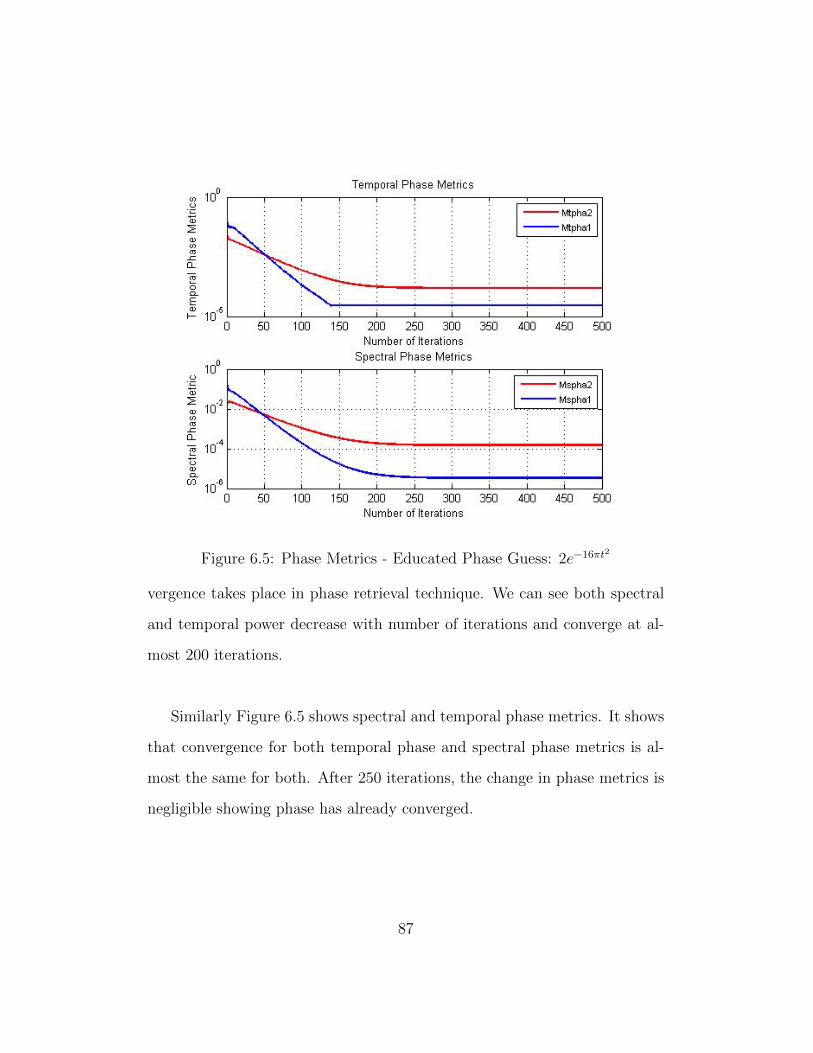
Figure 6.5: Phase Metrics - Educated Phase Guess: 2e−16πt2
vergence takes place in phase retrieval technique. We can see both spectral
and temporal power decrease with number of iterations and converge at al-
most 200 iterations.
Similarly Figure 6.5 shows spectral and temporal phase metrics. It shows
that convergence for both temporal phase and spectral phase metrics is al-
most the same for both. After 250 iterations, the change in phase metrics is
negligible showing phase has already converged.
87
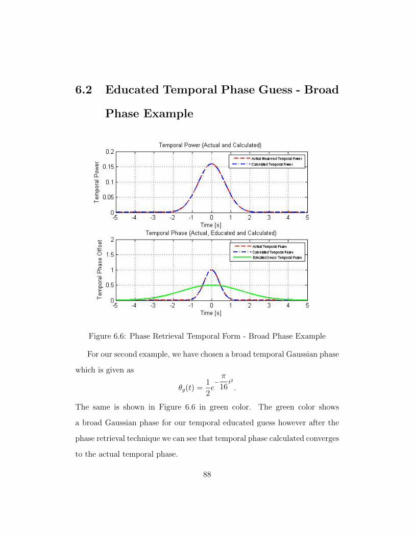
6.2 Educated Temporal Phase Guess - Broad
Phase Example
Figure 6.6: Phase Retrieval Temporal Form - Broad Phase Example
For our second example, we have chosen a broad temporal Gaussian phase
which is given as
θg(t) =1
2e−π
16t2
.
The same is shown in Figure 6.6 in green color. The green color shows
a broad Gaussian phase for our temporal educated guess however after the
phase retrieval technique we can see that temporal phase calculated converges
to the actual temporal phase.
88
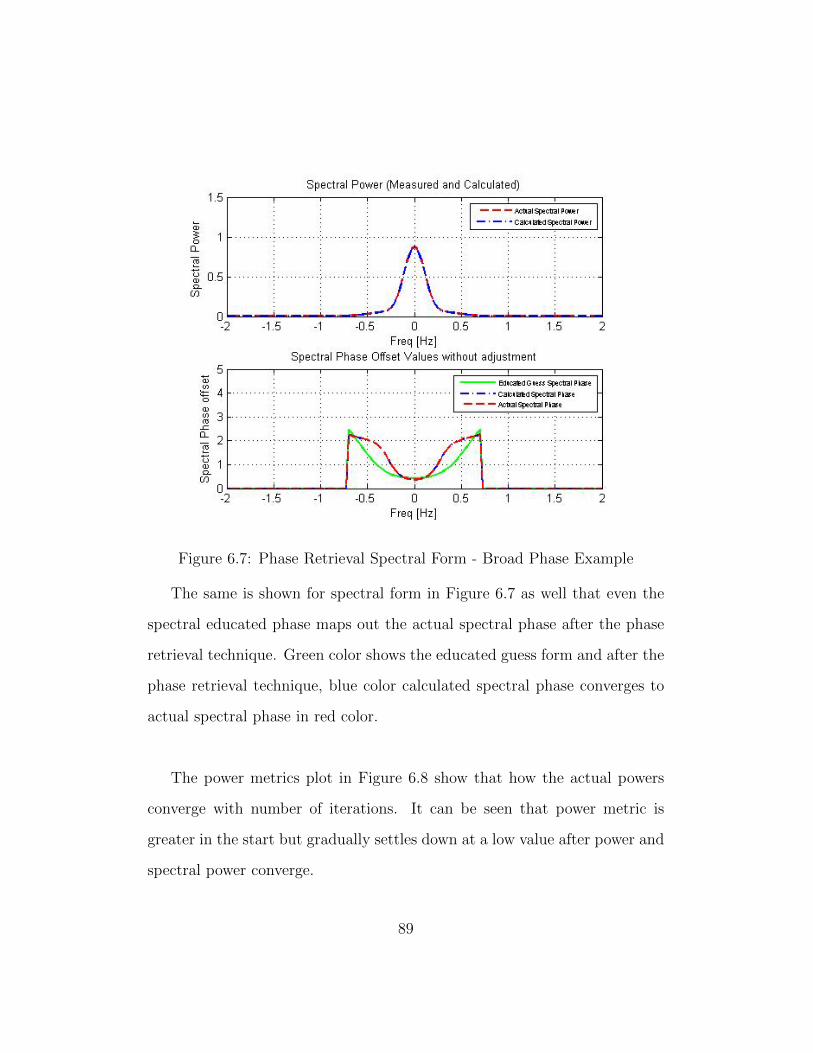
Figure 6.7: Phase Retrieval Spectral Form - Broad Phase Example
The same is shown for spectral form in Figure 6.7 as well that even the
spectral educated phase maps out the actual spectral phase after the phase
retrieval technique. Green color shows the educated guess form and after the
phase retrieval technique, blue color calculated spectral phase converges to
actual spectral phase in red color.
The power metrics plot in Figure 6.8 show that how the actual powers
converge with number of iterations. It can be seen that power metric is
greater in the start but gradually settles down at a low value after power and
spectral power converge.
89
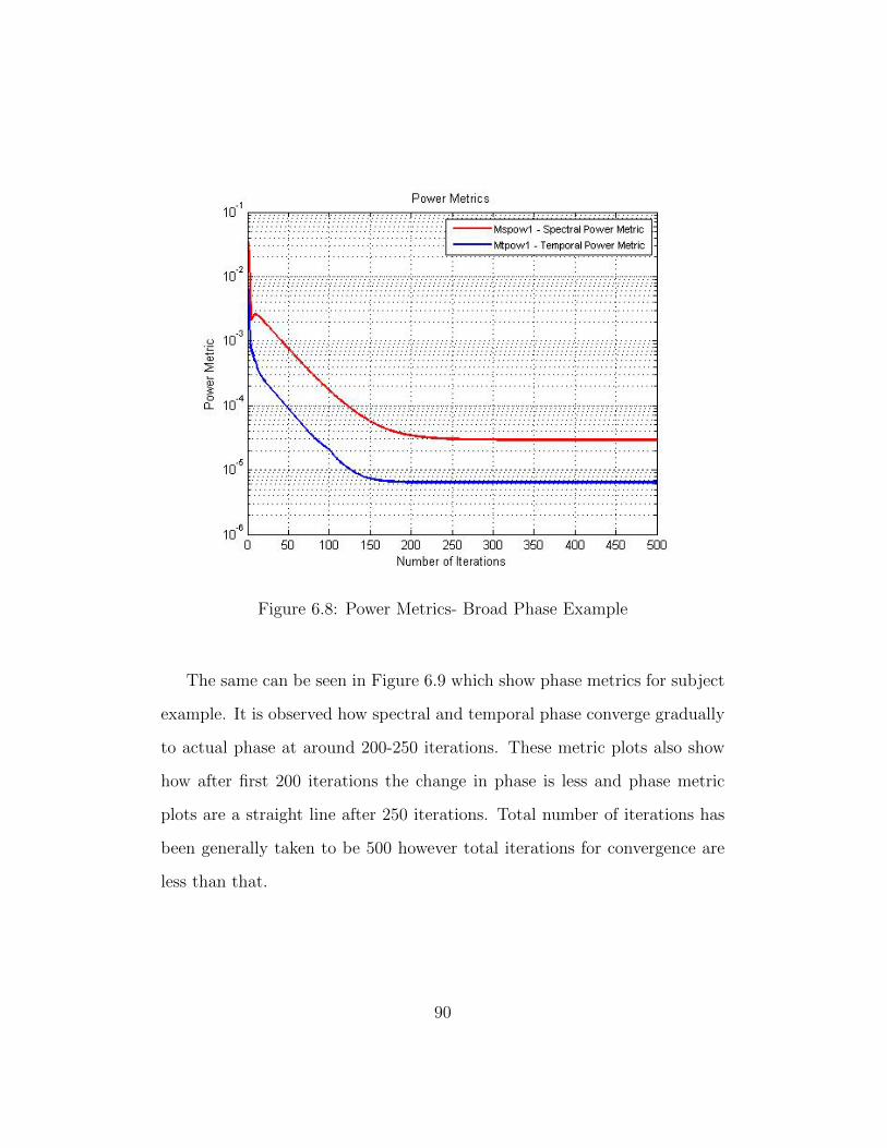
Figure 6.8: Power Metrics- Broad Phase Example
The same can be seen in Figure 6.9 which show phase metrics for subject
example. It is observed how spectral and temporal phase converge gradually
to actual phase at around 200-250 iterations. These metric plots also show
how after first 200 iterations the change in phase is less and phase metric
plots are a straight line after 250 iterations. Total number of iterations has
been generally taken to be 500 however total iterations for convergence are
less than that.
90
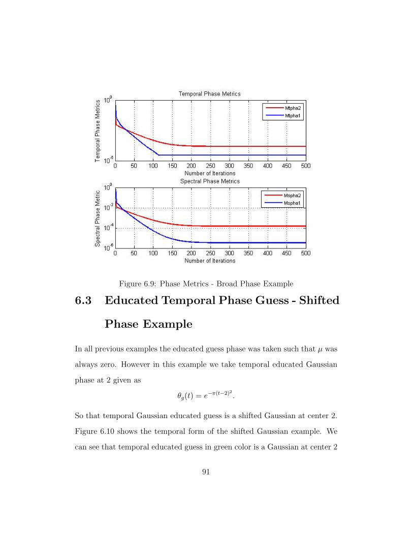
Figure 6.9: Phase Metrics - Broad Phase Example
6.3 Educated Temporal Phase Guess - Shifted
Phase Example
In all previous examples the educated guess phase was taken such that µ was
always zero. However in this example we take temporal educated Gaussian
phase at 2 given as
θg(t) = e−π(t−2)2
.
So that temporal Gaussian educated guess is a shifted Gaussian at center 2.
Figure 6.10 shows the temporal form of the shifted Gaussian example. We
can see that temporal educated guess in green color is a Gaussian at center 2
91
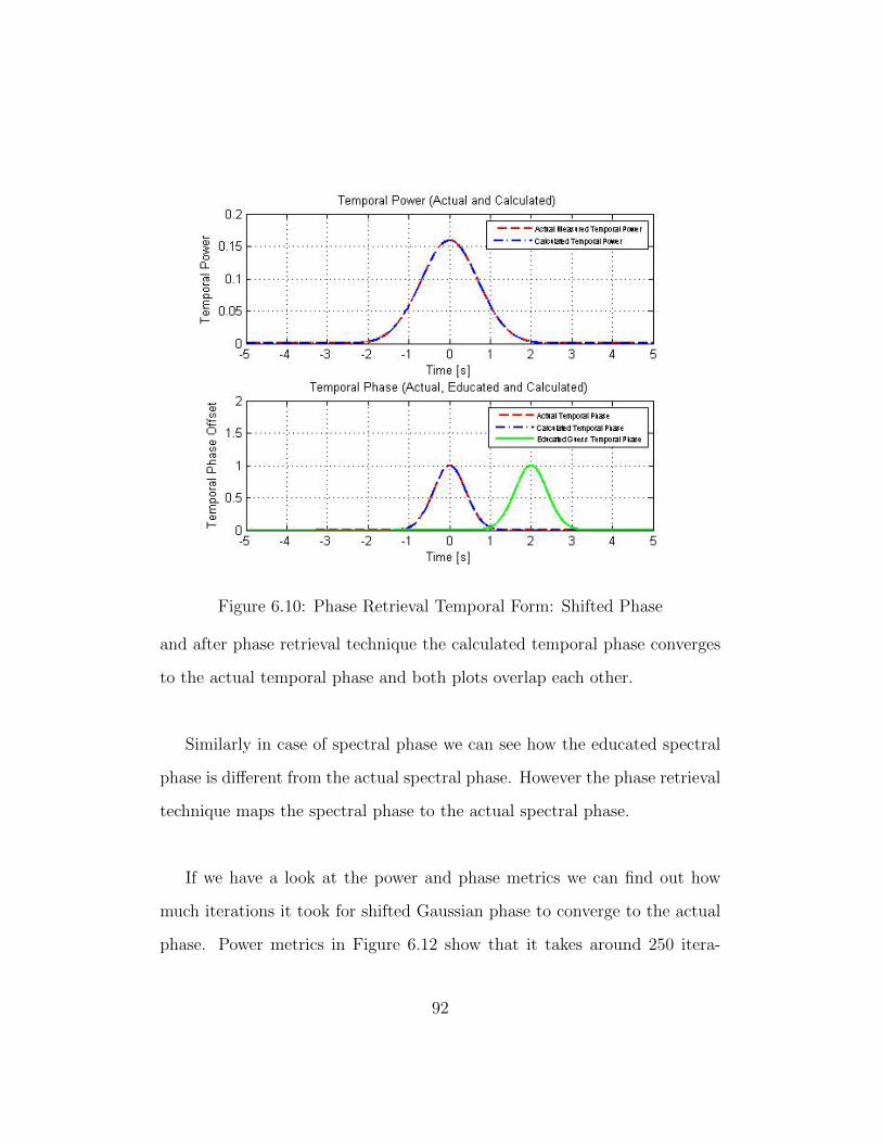
Figure 6.10: Phase Retrieval Temporal Form: Shifted Phase
and after phase retrieval technique the calculated temporal phase converges
to the actual temporal phase and both plots overlap each other.
Similarly in case of spectral phase we can see how the educated spectral
phase is different from the actual spectral phase. However the phase retrieval
technique maps the spectral phase to the actual spectral phase.
If we have a look at the power and phase metrics we can find out how
much iterations it took for shifted Gaussian phase to converge to the actual
phase. Power metrics in Figure 6.12 show that it takes around 250 itera-
92
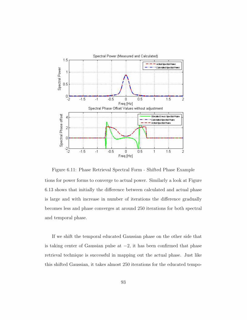
Figure 6.11: Phase Retrieval Spectral Form - Shifted Phase Example
tions for power forms to converge to actual power. Similarly a look at Figure
6.13 shows that initially the difference between calculated and actual phase
is large and with increase in number of iterations the difference gradually
becomes less and phase converges at around 250 iterations for both spectral
and temporal phase.
If we shift the temporal educated Gaussian phase on the other side that
is taking center of Gaussian pulse at −2, it has been confirmed that phase
retrieval technique is successful in mapping out the actual phase. Just like
this shifted Gaussian, it takes almost 250 iterations for the educated tempo-
93
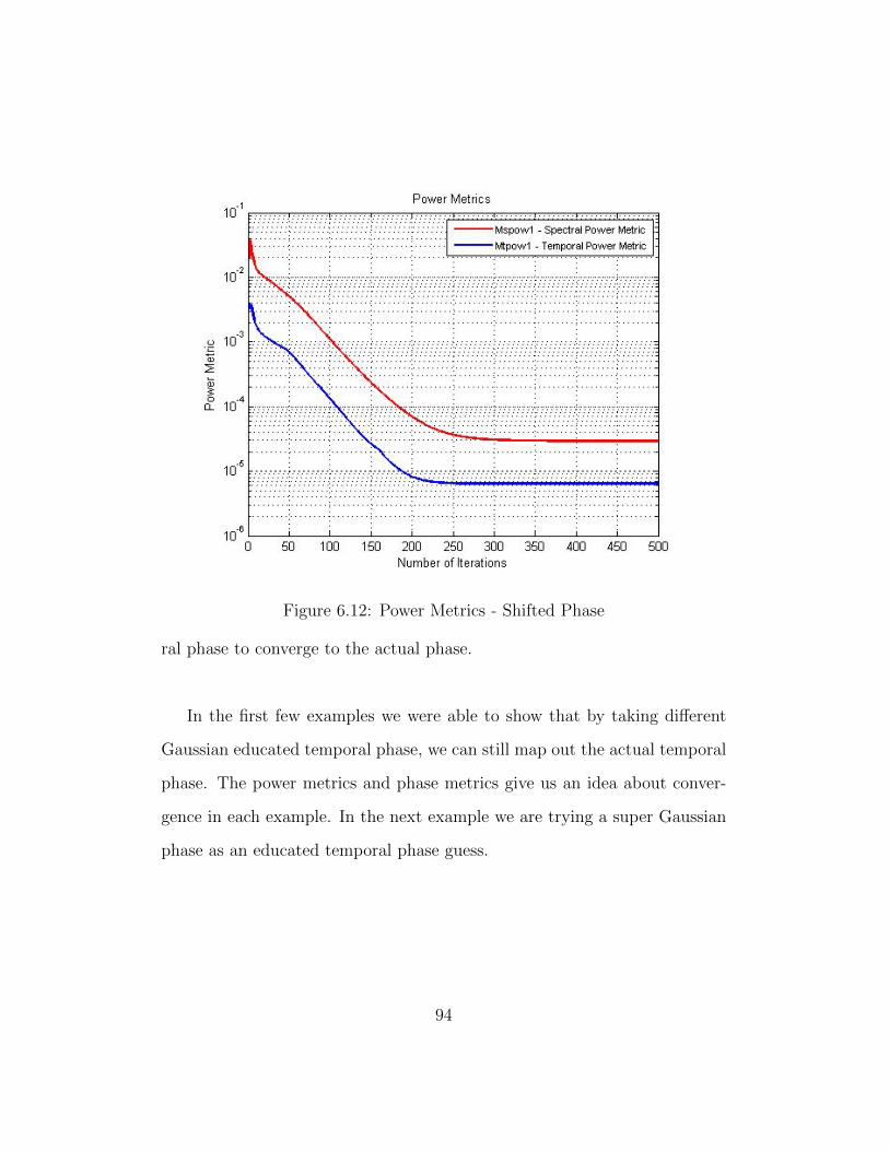
Figure 6.12: Power Metrics - Shifted Phase
ral phase to converge to the actual phase.
In the first few examples we were able to show that by taking different
Gaussian educated temporal phase, we can still map out the actual temporal
phase. The power metrics and phase metrics give us an idea about conver-
gence in each example. In the next example we are trying a super Gaussian
phase as an educated temporal phase guess.
94
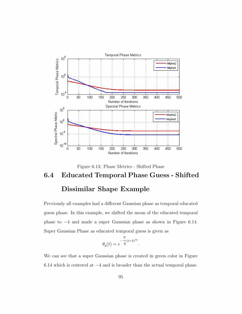
Figure 6.13: Phase Metrics - Shifted Phase
6.4 Educated Temporal Phase Guess - Shifted
Dissimilar Shape Example
Previously all examples had a different Gaussian phase as temporal educated
guess phase. In this example, we shifted the mean of the educated temporal
phase to −4 and made a super Gaussian phase as shown in Figure 6.14.
Super Gaussian Phase as educated temporal guess is given as
θg(t) = e−π
4(t+4)10
.
We can see that a super Gaussian phase is created in green color in Figure
6.14 which is centered at −4 and is broader than the actual temporal phase.
95
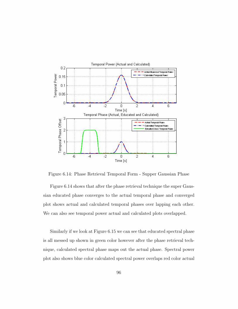
Figure 6.14: Phase Retrieval Temporal Form - Supper Gaussian Phase
Figure 6.14 shows that after the phase retrieval technique the super Gaus-
sian educated phase converges to the actual temporal phase and converged
plot shows actual and calculated temporal phases over lapping each other.
We can also see temporal power actual and calculated plots overlapped.
Similarly if we look at Figure 6.15 we can see that educated spectral phase
is all messed up shown in green color however after the phase retrieval tech-
nique, calculated spectral phase maps out the actual phase. Spectral power
plot also shows blue color calculated spectral power overlaps red color actual
96
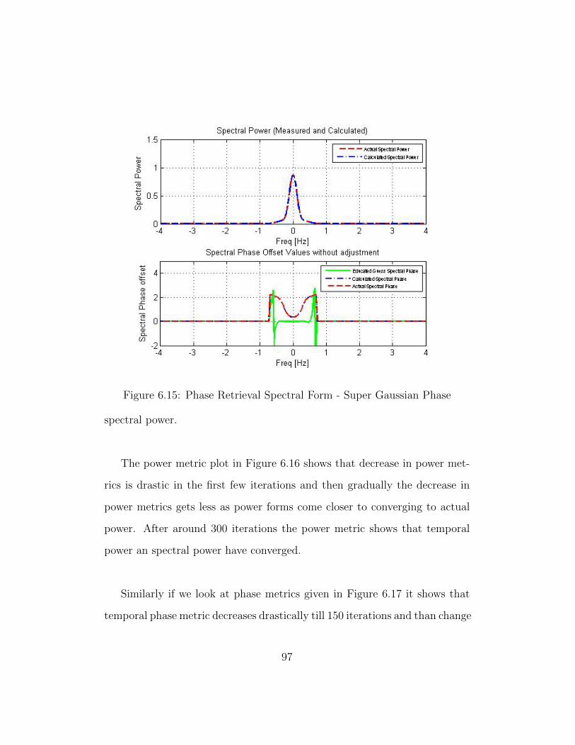
Figure 6.15: Phase Retrieval Spectral Form - Super Gaussian Phase
spectral power.
The power metric plot in Figure 6.16 shows that decrease in power met-
rics is drastic in the first few iterations and then gradually the decrease in
power metrics gets less as power forms come closer to converging to actual
power. After around 300 iterations the power metric shows that temporal
power an spectral power have converged.
Similarly if we look at phase metrics given in Figure 6.17 it shows that
temporal phase metric decreases drastically till 150 iterations and than change
97
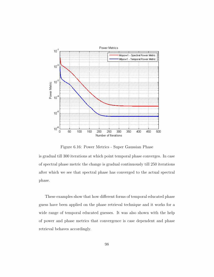
Figure 6.16: Power Metrics - Super Gaussian Phase
is gradual till 300 iterations at which point temporal phase converges. In case
of spectral phase metric the change is gradual continuously till 250 iterations
after which we see that spectral phase has converged to the actual spectral
phase.
These examples show that how different forms of temporal educated phase
guess have been applied on the phase retrieval technique and it works for a
wide range of temporal educated guesses. It was also shown with the help
of power and phase metrics that convergence is case dependent and phase
retrieval behaves accordingly.
98
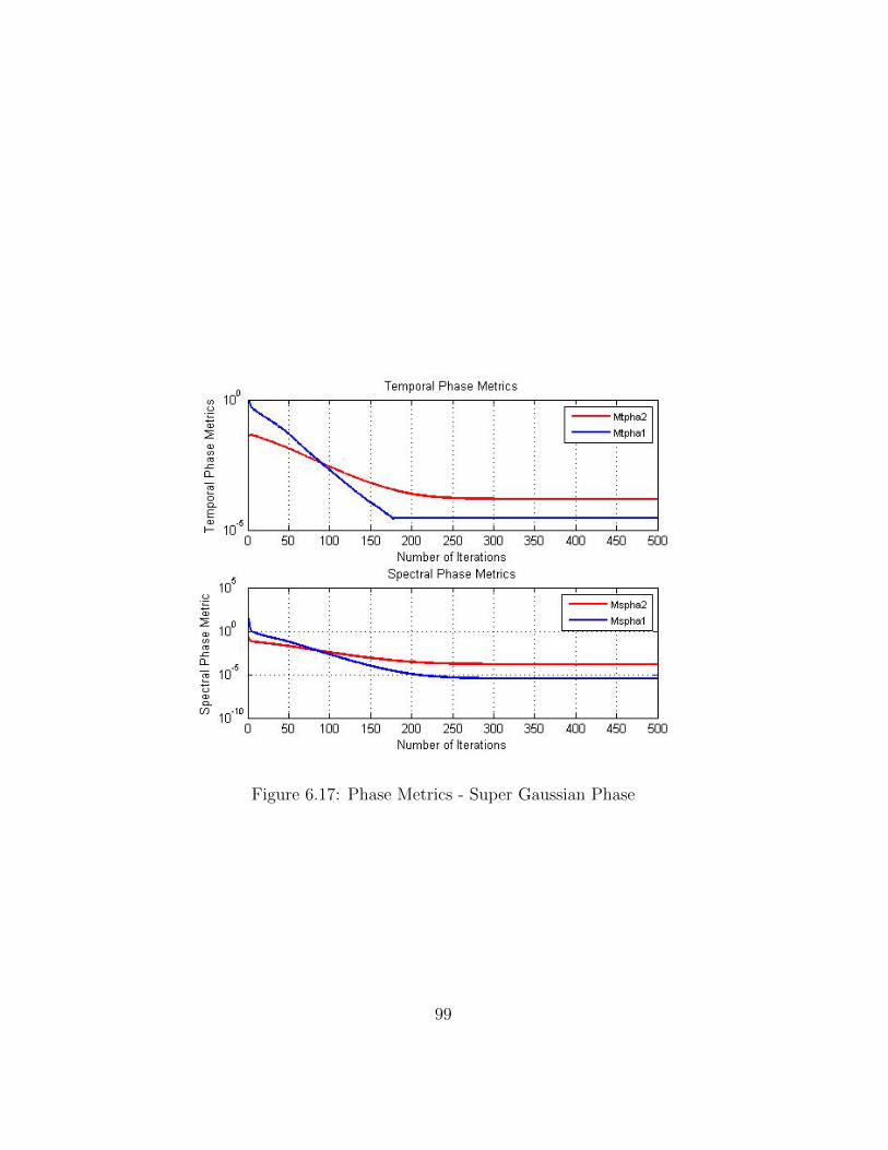
Figure 6.17: Phase Metrics - Super Gaussian Phase
99
Chapter 7
Phase Retrieval Technique for
Chirped Pulses
The Phase retrieval technique discussed so far has been applied using Gaus-
sian phase. Gaussian pulses have been used in setting up actual temporal
phase, for educated temporal phase a different type of Gaussian has been
chosen. In last chapter it was shown even when shifted Gaussian and Super
Gaussian pulses were used for educated temporal phase, the phase retrieval
technique does map educated temporal and spectral phases to their respec-
tive actual phase. In this chapter, we are going to study chirped pulses and
the phase retrieval technique’s response.
100

Figure 7.1: Temporal Optical Signal Power and Phase with C = 2
7.1 Defining Chirped Optical Pulse
Figure 7.1 shows a chirped actual temporal pulse which is being used for a
temporal optical signal. As we know that optical signal in time domain is
given by
E(t) =√P (t)eiθ(t)
where P (t) is the temporal power, θ(t) is the temporal phase. The high
speed optical carrier frequency is neglected here. For chirped pulses, actual
temporal phase is taken as following
θ(t) =−C(t− µ)2
2σ2
101
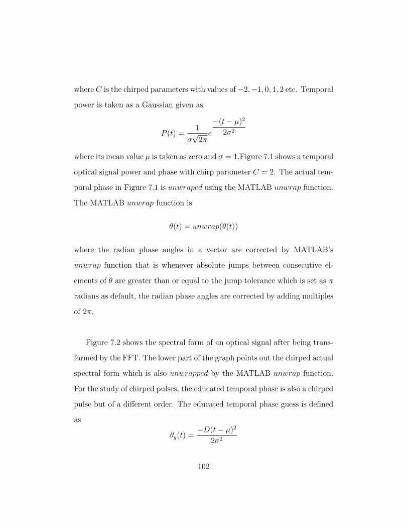
where C is the chirped parameters with values of−2,−1, 0, 1, 2 etc. Temporal
power is taken as a Gaussian given as
P (t) =1
σ√
2πe
−(t− µ)2
2σ2
where its mean value µ is taken as zero and σ = 1.Figure 7.1 shows a temporal
optical signal power and phase with chirp parameter C = 2. The actual tem-
poral phase in Figure 7.1 is unwraped using the MATLAB unwrap function.
The MATLAB unwrap function is
θ(t) = unwrap(θ(t))
where the radian phase angles in a vector are corrected by MATLAB’s
unwrap function that is whenever absolute jumps between consecutive el-
ements of θ are greater than or equal to the jump tolerance which is set as π
radians as default, the radian phase angles are corrected by adding multiples
of 2π.
Figure 7.2 shows the spectral form of an optical signal after being trans-
formed by the FFT. The lower part of the graph points out the chirped actual
spectral form which is also unwrapped by the MATLAB unwrap function.
For the study of chirped pulses, the educated temporal phase is also a chirped
pulse but of a different order. The educated temporal phase guess is defined
as
θg(t) =−D(t− µ)2
2σ2
102
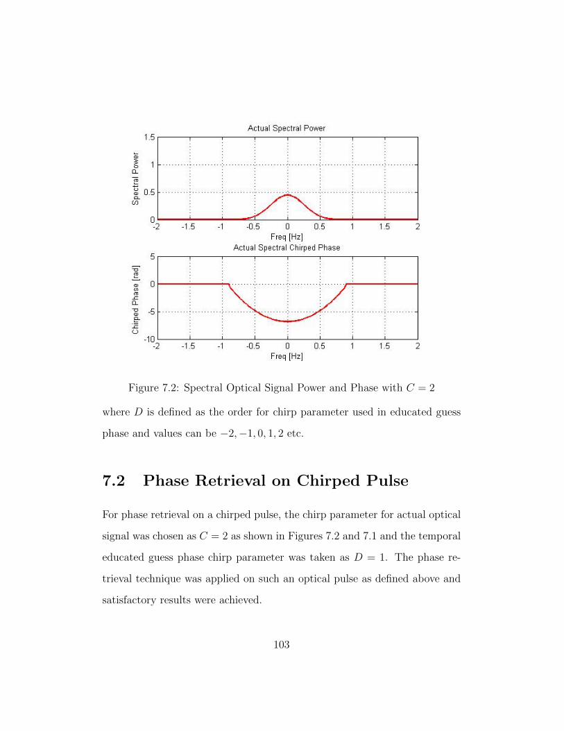
Figure 7.2: Spectral Optical Signal Power and Phase with C = 2
where D is defined as the order for chirp parameter used in educated guess
phase and values can be −2,−1, 0, 1, 2 etc.
7.2 Phase Retrieval on Chirped Pulse
For phase retrieval on a chirped pulse, the chirp parameter for actual optical
signal was chosen as C = 2 as shown in Figures 7.2 and 7.1 and the temporal
educated guess phase chirp parameter was taken as D = 1. The phase re-
trieval technique was applied on such an optical pulse as defined above and
satisfactory results were achieved.
103
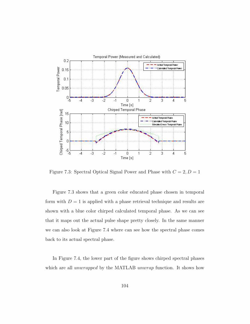
Figure 7.3: Spectral Optical Signal Power and Phase with C = 2, D = 1
Figure 7.3 shows that a green color educated phase chosen in temporal
form with D = 1 is applied with a phase retrieval technique and results are
shown with a blue color chirped calculated temporal phase. As we can see
that it maps out the actual pulse shape pretty closely. In the same manner
we can also look at Figure 7.4 where can see how the spectral phase comes
back to its actual spectral phase.
In Figure 7.4, the lower part of the figure shows chirped spectral phases
which are all unwrapped by the MATLAB unwrap function. It shows how
104
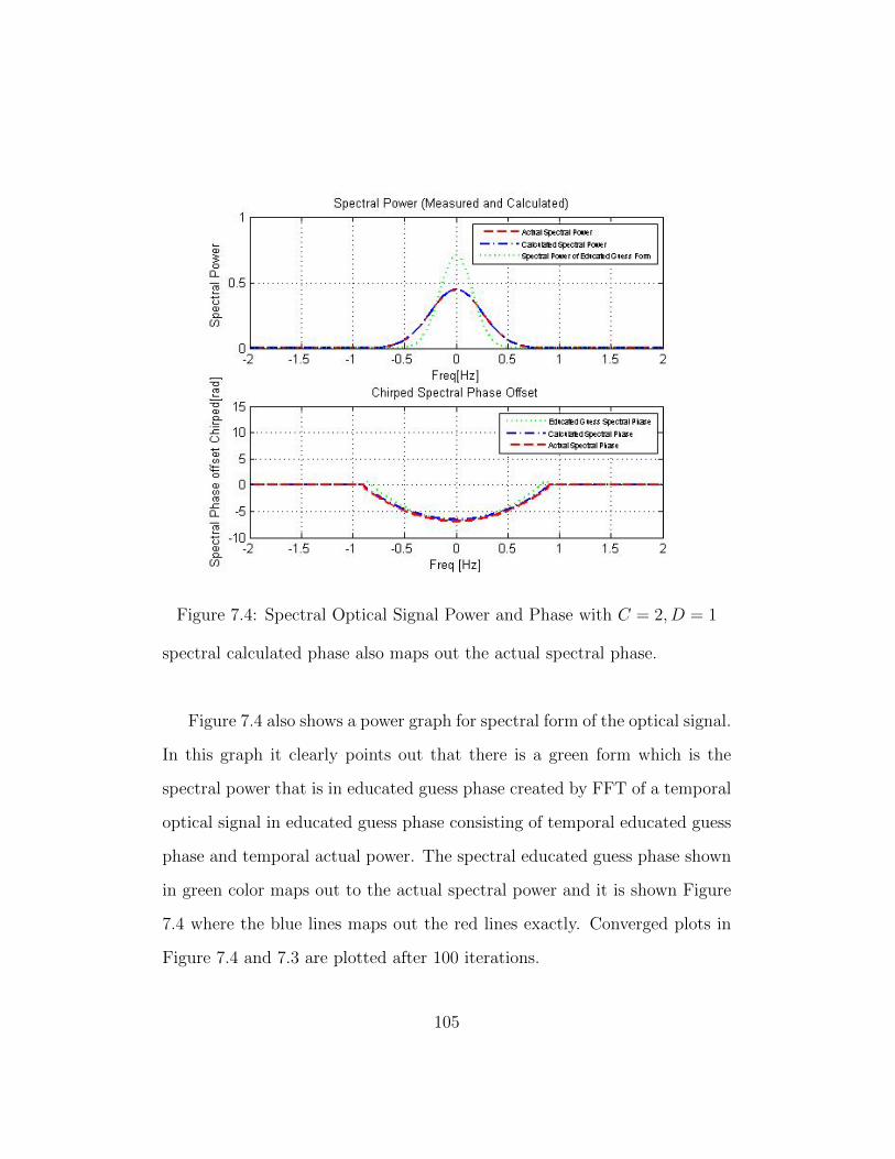
Figure 7.4: Spectral Optical Signal Power and Phase with C = 2, D = 1
spectral calculated phase also maps out the actual spectral phase.
Figure 7.4 also shows a power graph for spectral form of the optical signal.
In this graph it clearly points out that there is a green form which is the
spectral power that is in educated guess phase created by FFT of a temporal
optical signal in educated guess phase consisting of temporal educated guess
phase and temporal actual power. The spectral educated guess phase shown
in green color maps out to the actual spectral power and it is shown Figure
7.4 where the blue lines maps out the red lines exactly. Converged plots in
Figure 7.4 and 7.3 are plotted after 100 iterations.
105
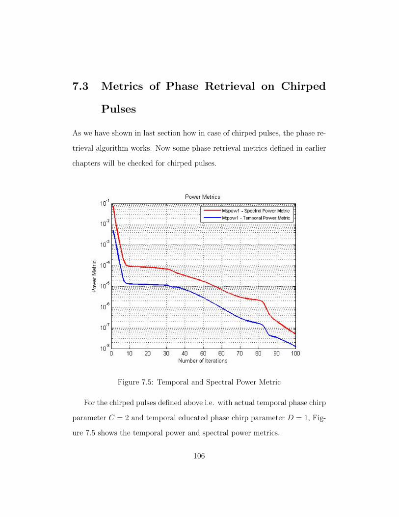
7.3 Metrics of Phase Retrieval on Chirped
Pulses
As we have shown in last section how in case of chirped pulses, the phase re-
trieval algorithm works. Now some phase retrieval metrics defined in earlier
chapters will be checked for chirped pulses.
Figure 7.5: Temporal and Spectral Power Metric
For the chirped pulses defined above i.e. with actual temporal phase chirp
parameter C = 2 and temporal educated phase chirp parameter D = 1, Fig-
ure 7.5 shows the temporal power and spectral power metrics.
106
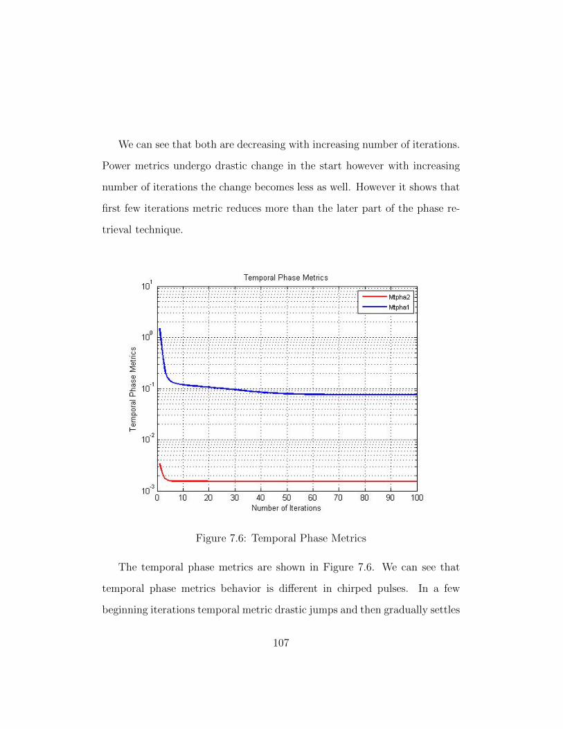
We can see that both are decreasing with increasing number of iterations.
Power metrics undergo drastic change in the start however with increasing
number of iterations the change becomes less as well. However it shows that
first few iterations metric reduces more than the later part of the phase re-
trieval technique.
Figure 7.6: Temporal Phase Metrics
The temporal phase metrics are shown in Figure 7.6. We can see that
temporal phase metrics behavior is different in chirped pulses. In a few
beginning iterations temporal metric drastic jumps and then gradually settles
107
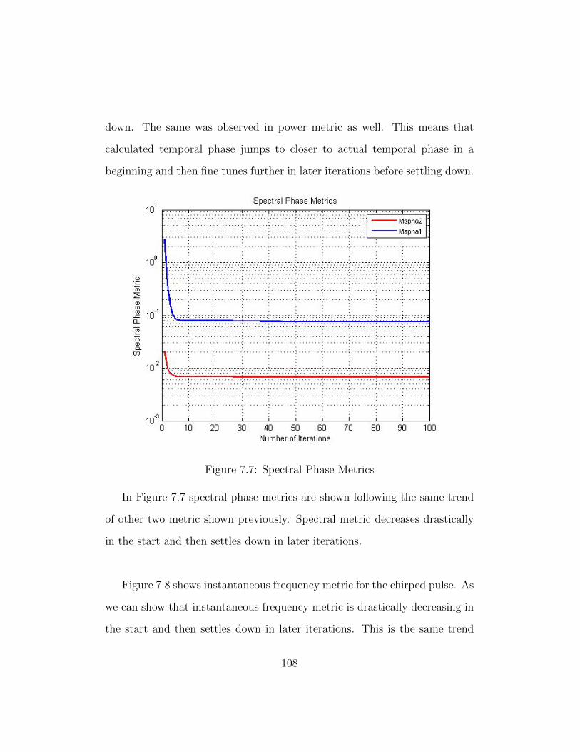
down. The same was observed in power metric as well. This means that
calculated temporal phase jumps to closer to actual temporal phase in a
beginning and then fine tunes further in later iterations before settling down.
Figure 7.7: Spectral Phase Metrics
In Figure 7.7 spectral phase metrics are shown following the same trend
of other two metric shown previously. Spectral metric decreases drastically
in the start and then settles down in later iterations.
Figure 7.8 shows instantaneous frequency metric for the chirped pulse. As
we can show that instantaneous frequency metric is drastically decreasing in
the start and then settles down in later iterations. This is the same trend
108
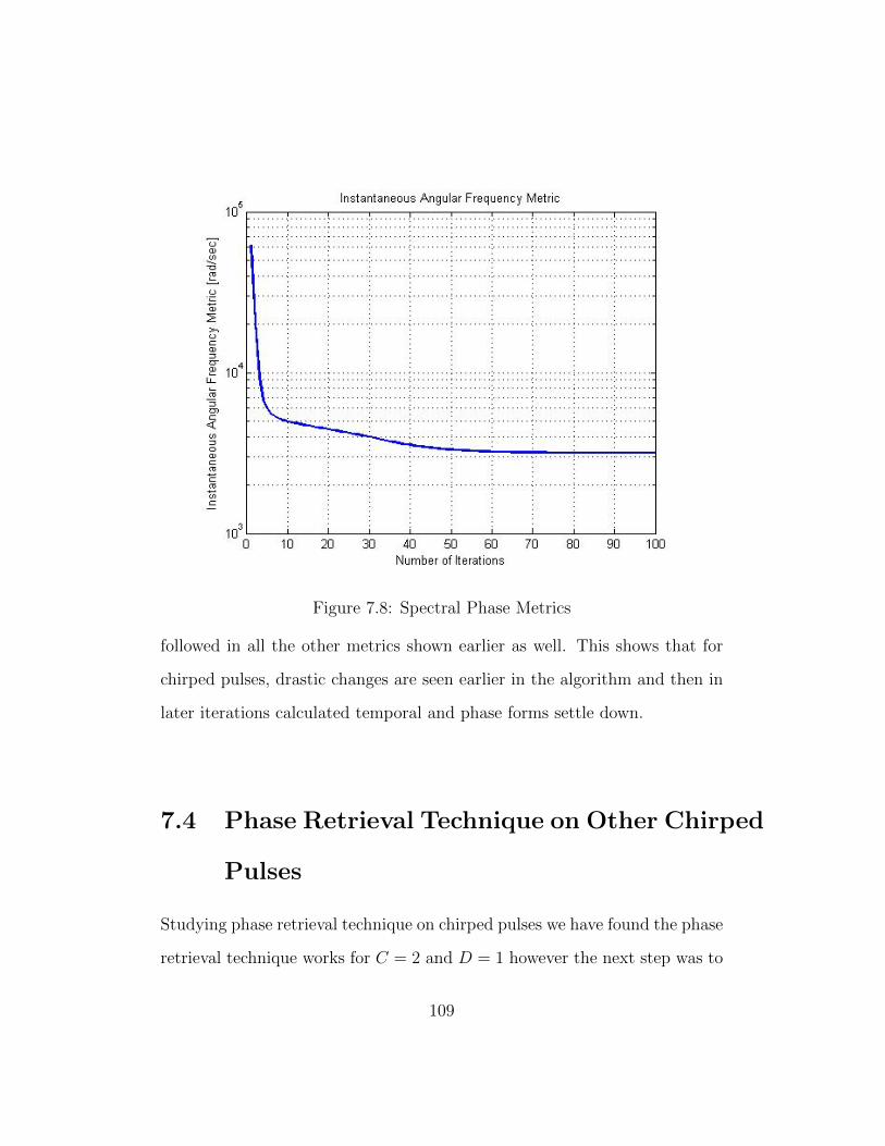
Figure 7.8: Spectral Phase Metrics
followed in all the other metrics shown earlier as well. This shows that for
chirped pulses, drastic changes are seen earlier in the algorithm and then in
later iterations calculated temporal and phase forms settle down.
7.4 Phase Retrieval Technique on Other Chirped
Pulses
Studying phase retrieval technique on chirped pulses we have found the phase
retrieval technique works for C = 2 and D = 1 however the next step was to
109
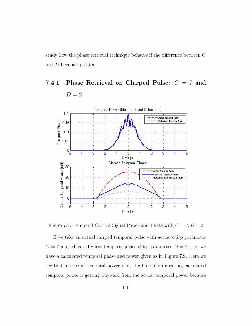
study how the phase retrieval technique behaves if the difference between C
and D becomes greater.
7.4.1 Phase Retrieval on Chirped Pulse: C = 7 and
D = 2
Figure 7.9: Temporal Optical Signal Power and Phase with C = 7, D = 2
If we take an actual chirped temporal pulse with actual chirp parameter
C = 7 and educated guess temporal phase chirp parameter D = 2 then we
have a calculated temporal phase and power given as in Figure 7.9. Here we
see that in case of temporal power plot, the blue line indicating calculated
temporal power is getting wayward from the actual temporal power because
110

of the huge difference between actual chirp parameter and educated guess
chirp paramter.
Figure 7.10: Power metric: Chirped Pulse with C = 7, D = 2
Similarly if we look at the lower plot of Figure 7.9 where we are plotting
temporal phase forms, it can be seen that calculated temporal form is having
a different phase and an unusual dip in the center as well which is not found
in actual temporal phase form.
Moreover we can study metrics in chirped pulse cases as they are showing
major changes indicating that phase retrieval technique has certain barriers
in which it works perfect for chirped pulses before going wayward. Consider
111
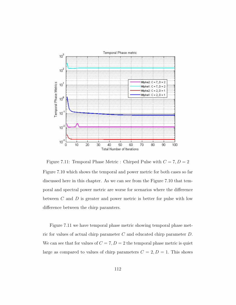
Figure 7.11: Temporal Phase Metric : Chirped Pulse with C = 7, D = 2
Figure 7.10 which shows the temporal and power metric for both cases so far
discussed here in this chapter. As we can see from the Figure 7.10 that tem-
poral and spectral power metric are worse for scenarios where the difference
between C and D is greater and power metric is better for pulse with low
difference between the chirp paramters.
Figure 7.11 we have temporal phase metric showing temporal phase met-
ric for values of actual chirp parameter C and educated chirp parameter D.
We can see that for values of C = 7, D = 2 the temporal phase metric is quiet
large as compared to values of chirp parameters C = 2, D = 1. This shows
112
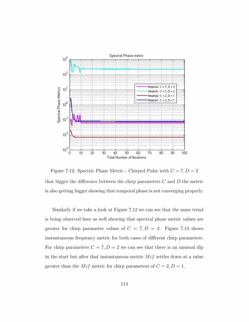
Figure 7.12: Spectric Phase Metric : Chirped Pulse with C = 7, D = 2
that bigger the difference between the chirp parameters C and D the metric
is also getting bigger showing that temporal phase is not converging properly.
Similarly if we take a look at Figure 7.12 we can see that the same trend
is being observed here as well showing that spectral phase metric values are
greater for chirp parameter values of C = 7, D = 2. Figure 7.13 shows
instantaneous frequency metric for both cases of different chirp parameters.
For chirp parameters C = 7, D = 2 we can see that there is an unusual dip
in the start but after that instantaneous metric Mif settles down at a value
greater than the Mif metric for chirp parameters of C = 2, D = 1.
113
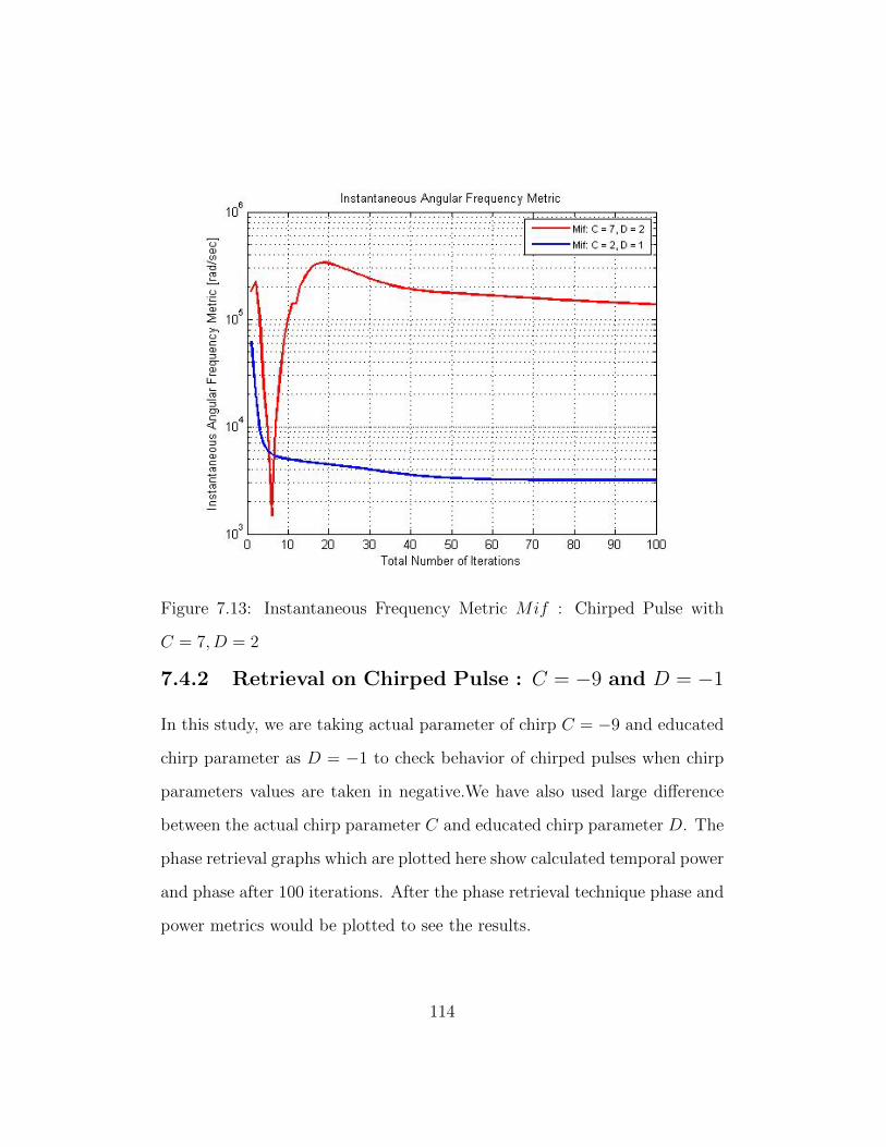
Figure 7.13: Instantaneous Frequency Metric Mif : Chirped Pulse with
C = 7, D = 2
7.4.2 Retrieval on Chirped Pulse : C = −9 and D = −1
In this study, we are taking actual parameter of chirp C = −9 and educated
chirp parameter as D = −1 to check behavior of chirped pulses when chirp
parameters values are taken in negative.We have also used large difference
between the actual chirp parameter C and educated chirp parameter D. The
phase retrieval graphs which are plotted here show calculated temporal power
and phase after 100 iterations. After the phase retrieval technique phase and
power metrics would be plotted to see the results.
114
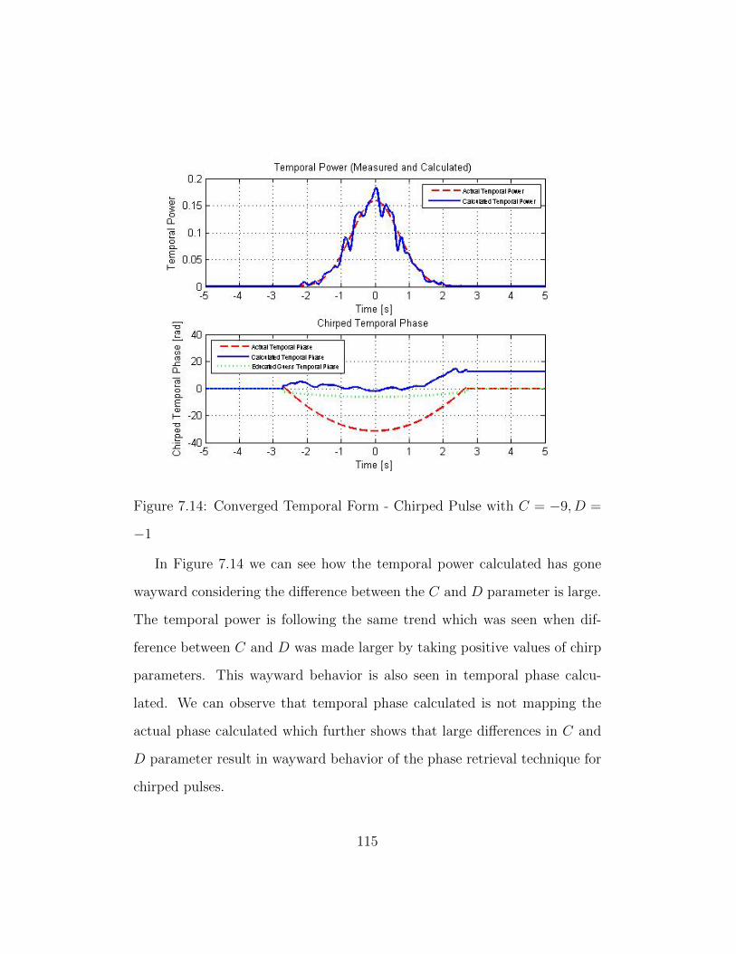
Figure 7.14: Converged Temporal Form - Chirped Pulse with C = −9, D =
−1
In Figure 7.14 we can see how the temporal power calculated has gone
wayward considering the difference between the C and D parameter is large.
The temporal power is following the same trend which was seen when dif-
ference between C and D was made larger by taking positive values of chirp
parameters. This wayward behavior is also seen in temporal phase calcu-
lated. We can observe that temporal phase calculated is not mapping the
actual phase calculated which further shows that large differences in C and
D parameter result in wayward behavior of the phase retrieval technique for
chirped pulses.
115
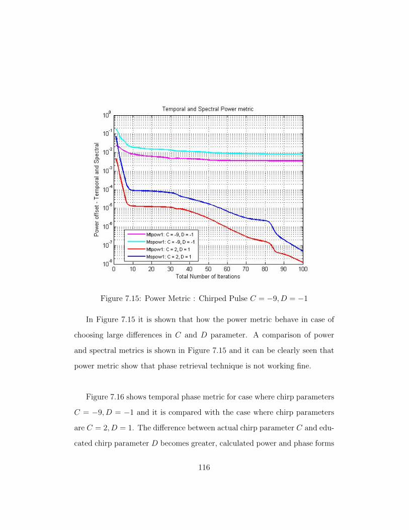
Figure 7.15: Power Metric : Chirped Pulse C = −9, D = −1
In Figure 7.15 it is shown that how the power metric behave in case of
choosing large differences in C and D parameter. A comparison of power
and spectral metrics is shown in Figure 7.15 and it can be clearly seen that
power metric show that phase retrieval technique is not working fine.
Figure 7.16 shows temporal phase metric for case where chirp parameters
C = −9, D = −1 and it is compared with the case where chirp parameters
are C = 2, D = 1. The difference between actual chirp parameter C and edu-
cated chirp parameter D becomes greater, calculated power and phase forms
116
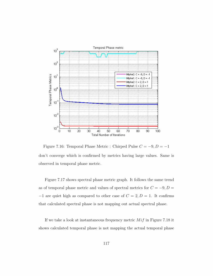
Figure 7.16: Temporal Phase Metric : Chirped Pulse C = −9, D = −1
don’t converge which is confirmed by metrics having large values. Same is
observed in temporal phase metric.
Figure 7.17 shows spectral phase metric graph. It follows the same trend
as of temporal phase metric and values of spectral metrics for C = −9, D =
−1 are quiet high as compared to other case of C = 2, D = 1. It confirms
that calculated spectral phase is not mapping out actual spectral phase.
If we take a look at instantaneous frequency metric Mif in Figure 7.18 it
shows calculated temporal phase is not mapping the actual temporal phase
117

Figure 7.17: Spectral Phase Metric : Chirped Pulse C = −9, D = −1
for cases of C = −9, D = −1. Mif metric is messed up showing wayward
behavior of calculated phase.
In all the metrics shown above, the trend has been the same that if the
difference between actual chirp parameter C and educated chirp parameter
D is greater then the temporal and power forms do not map the actual forms
perfectly and the same is confirmed by checking power and phase metrics.
118
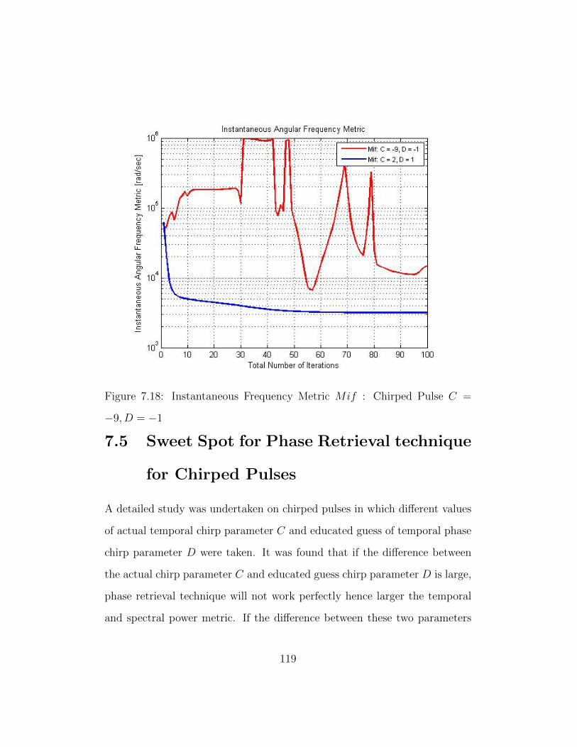
Figure 7.18: Instantaneous Frequency Metric Mif : Chirped Pulse C =
−9, D = −1
7.5 Sweet Spot for Phase Retrieval technique
for Chirped Pulses
A detailed study was undertaken on chirped pulses in which different values
of actual temporal chirp parameter C and educated guess of temporal phase
chirp parameter D were taken. It was found that if the difference between
the actual chirp parameter C and educated guess chirp parameter D is large,
phase retrieval technique will not work perfectly hence larger the temporal
and spectral power metric. If the difference between these two parameters
119
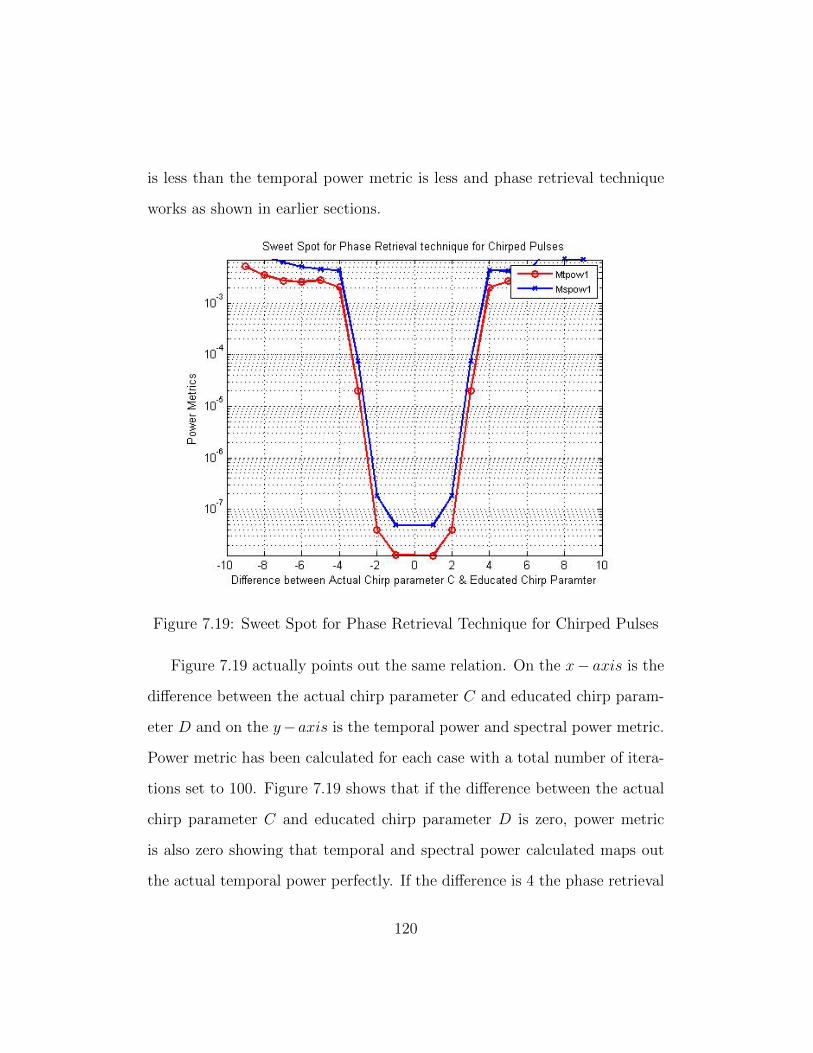
is less than the temporal power metric is less and phase retrieval technique
works as shown in earlier sections.
Figure 7.19: Sweet Spot for Phase Retrieval Technique for Chirped Pulses
Figure 7.19 actually points out the same relation. On the x− axis is the
difference between the actual chirp parameter C and educated chirp param-
eter D and on the y−axis is the temporal power and spectral power metric.
Power metric has been calculated for each case with a total number of itera-
tions set to 100. Figure 7.19 shows that if the difference between the actual
chirp parameter C and educated chirp parameter D is zero, power metric
is also zero showing that temporal and spectral power calculated maps out
the actual temporal power perfectly. If the difference is 4 the phase retrieval
120

technique does work but there are some differences in the actual temporal
power and calculated temporal power and similarly in temporal phase forms
as well. However if the difference gets larger to 8 the phase retrieval technique
doesn’t respond well. This gives us a sweet spot right in the middle of the
Figure 7.19 showing that if the difference between actual chirp parameter C
and educated chirp parameter D is between 0 to 4 phase retrieval technique
will respond well otherwise it won’t give desired results.
121
Chapter 8
Phase Retrieval of Chirped
Super Gaussian Pulses
In the last chapter we discussed about phase retrieval technique on chirped
pulses. We figured out the phase retrieval technique for chirped pulses works
well when the difference between the actual chirp parameter C and educated
guess chirp parameter D is small. In this chapter we are going to study the
phase retrieval technique on chirped super Gaussian pulses.
8.1 Chirped Super Gaussian Pulse
As we know that the optical signal in temporal domain is given by
E(t) =√P (t)eiθ(t)
122
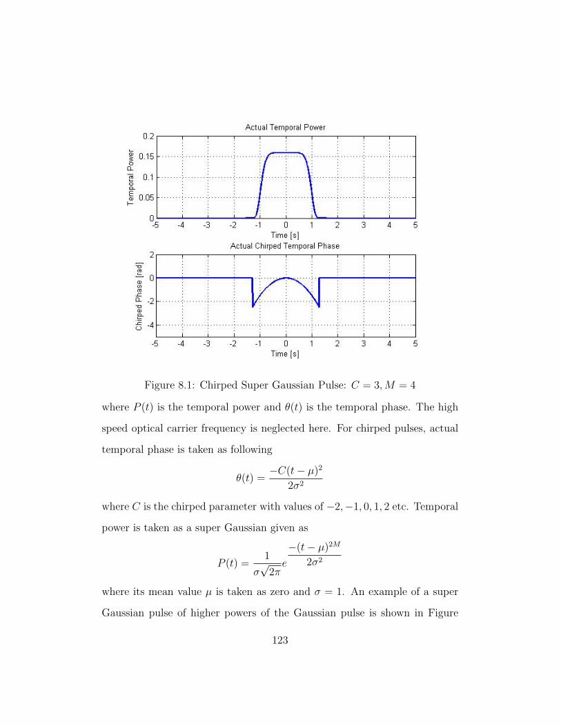
Figure 8.1: Chirped Super Gaussian Pulse: C = 3,M = 4
where P (t) is the temporal power and θ(t) is the temporal phase. The high
speed optical carrier frequency is neglected here. For chirped pulses, actual
temporal phase is taken as following
θ(t) =−C(t− µ)2
2σ2
where C is the chirped parameter with values of −2,−1, 0, 1, 2 etc. Temporal
power is taken as a super Gaussian given as
P (t) =1
σ√
2πe
−(t− µ)2M
2σ2
where its mean value µ is taken as zero and σ = 1. An example of a super
Gaussian pulse of higher powers of the Gaussian pulse is shown in Figure
123
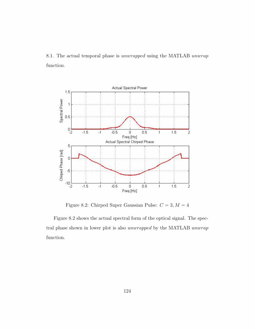
8.1. The actual temporal phase is unwrapped using the MATLAB unwrap
function.
Figure 8.2: Chirped Super Gaussian Pulse: C = 3,M = 4
Figure 8.2 shows the actual spectral form of the optical signal. The spec-
tral phase shown in lower plot is also unwrapped by the MATLAB unwrap
function.
124
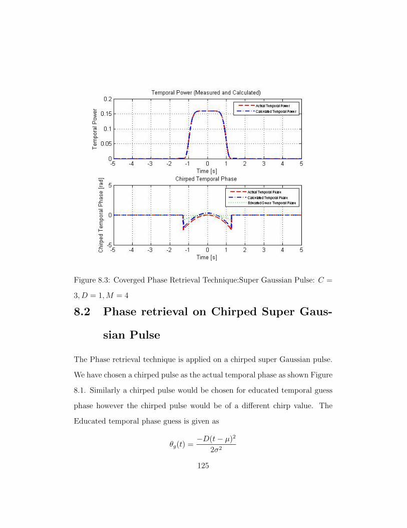
Figure 8.3: Coverged Phase Retrieval Technique:Super Gaussian Pulse: C =
3, D = 1,M = 4
8.2 Phase retrieval on Chirped Super Gaus-
sian Pulse
The Phase retrieval technique is applied on a chirped super Gaussian pulse.
We have chosen a chirped pulse as the actual temporal phase as shown Figure
8.1. Similarly a chirped pulse would be chosen for educated temporal guess
phase however the chirped pulse would be of a different chirp value. The
Educated temporal phase guess is given as
θg(t) =−D(t− µ)2
2σ2
125
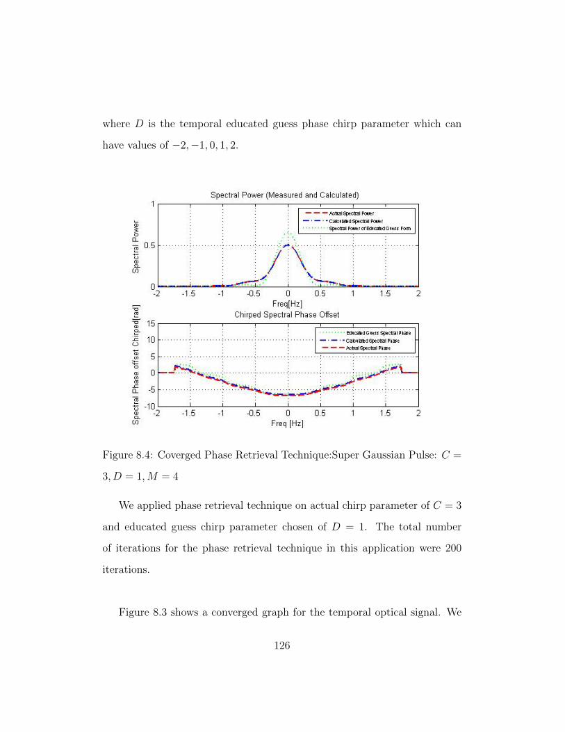
where D is the temporal educated guess phase chirp parameter which can
have values of −2,−1, 0, 1, 2.
Figure 8.4: Coverged Phase Retrieval Technique:Super Gaussian Pulse: C =
3, D = 1,M = 4
We applied phase retrieval technique on actual chirp parameter of C = 3
and educated guess chirp parameter chosen of D = 1. The total number
of iterations for the phase retrieval technique in this application were 200
iterations.
Figure 8.3 shows a converged graph for the temporal optical signal. We
126
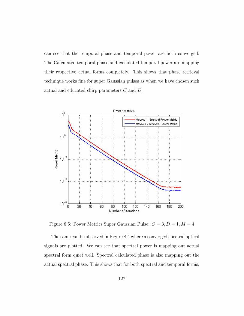
can see that the temporal phase and temporal power are both converged.
The Calculated temporal phase and calculated temporal power are mapping
their respective actual forms completely. This shows that phase retrieval
technique works fine for super Gaussian pulses as when we have chosen such
actual and educated chirp parameters C and D.
Figure 8.5: Power Metrics:Super Gaussian Pulse: C = 3, D = 1,M = 4
The same can be observed in Figure 8.4 where a converged spectral optical
signals are plotted. We can see that spectral power is mapping out actual
spectral form quiet well. Spectral calculated phase is also mapping out the
actual spectral phase. This shows that for both spectral and temporal forms,
127
phase retrieval technique is working.
8.3 Metrics of Phase Retrieval on Chirped
Super Gaussian Pulse
In the previous section we plotted actual and calculated forms of the chirped
super Gaussian pulse. In this section we will see how the different metrics
defined for our phase retrieval technique behave in the case of phase retrieval
on chirped super Gaussian pulse.
8.3.1 Power Metrics
We have defined two types of power metrics i.e. a temporal power metric
Mtpow1 and a spectral power metric Mspow1. Both of these are plotted in
Figure 8.5. We can see that both spectral and temporal power metrics are
decreasing in the start showing that power and temporal forms converge to
the temporal and spectral forms with very small metric values. Around after
150 iterations the power metrics gradually settle down.
8.3.2 Phase Metrics
In the same way we can have a look at the phase metrics of the phase retrieval
technique on a chirped super Gaussian pulse. We can see that the values of
both phase metrics are decreasing in the start and then after some iterations
they settle down. Both spectral and phase metrics are following the same
128
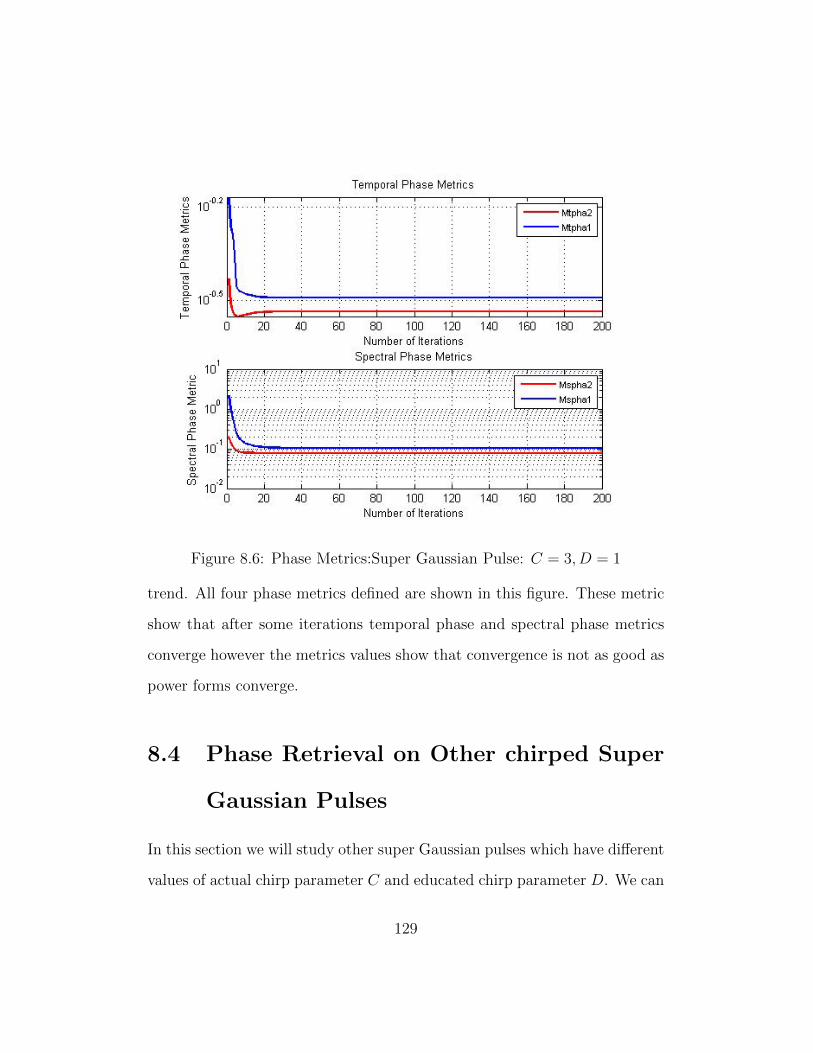
Figure 8.6: Phase Metrics:Super Gaussian Pulse: C = 3, D = 1
trend. All four phase metrics defined are shown in this figure. These metric
show that after some iterations temporal phase and spectral phase metrics
converge however the metrics values show that convergence is not as good as
power forms converge.
8.4 Phase Retrieval on Other chirped Super
Gaussian Pulses
In this section we will study other super Gaussian pulses which have different
values of actual chirp parameter C and educated chirp parameter D. We can
129
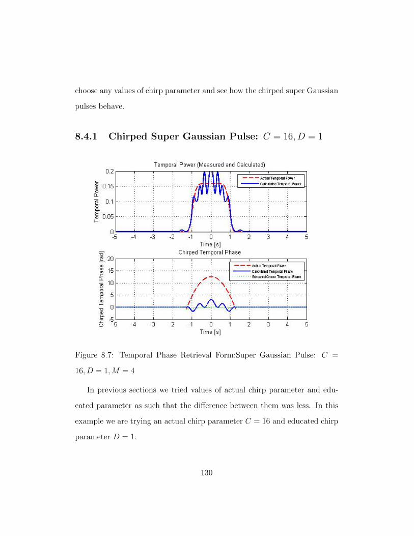
choose any values of chirp parameter and see how the chirped super Gaussian
pulses behave.
8.4.1 Chirped Super Gaussian Pulse: C = 16, D = 1
Figure 8.7: Temporal Phase Retrieval Form:Super Gaussian Pulse: C =
16, D = 1,M = 4
In previous sections we tried values of actual chirp parameter and edu-
cated parameter as such that the difference between them was less. In this
example we are trying an actual chirp parameter C = 16 and educated chirp
parameter D = 1.
130
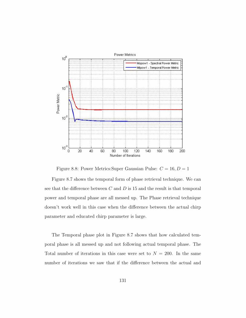
Figure 8.8: Power Metrics:Super Gaussian Pulse: C = 16, D = 1
Figure 8.7 shows the temporal form of phase retrieval technique. We can
see that the difference between C and D is 15 and the result is that temporal
power and temporal phase are all messed up. The Phase retrieval technique
doesn’t work well in this case when the difference between the actual chirp
parameter and educated chirp parameter is large.
The Temporal phase plot in Figure 8.7 shows that how calculated tem-
poral phase is all messed up and not following actual temporal phase. The
Total number of iterations in this case were set to N = 200. In the same
number of iterations we saw that if the difference between the actual and
131
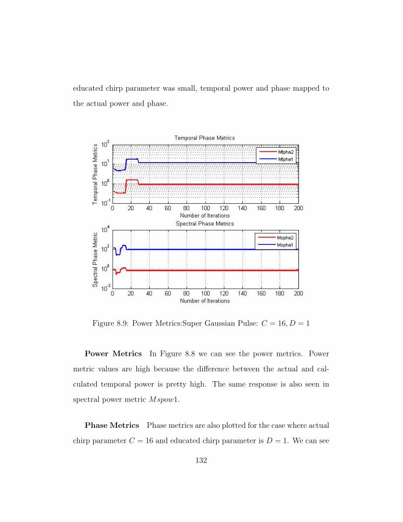
educated chirp parameter was small, temporal power and phase mapped to
the actual power and phase.
Figure 8.9: Power Metrics:Super Gaussian Pulse: C = 16, D = 1
Power Metrics In Figure 8.8 we can see the power metrics. Power
metric values are high because the difference between the actual and cal-
culated temporal power is pretty high. The same response is also seen in
spectral power metric Mspow1.
Phase Metrics Phase metrics are also plotted for the case where actual
chirp parameter C = 16 and educated chirp parameter is D = 1. We can see
132
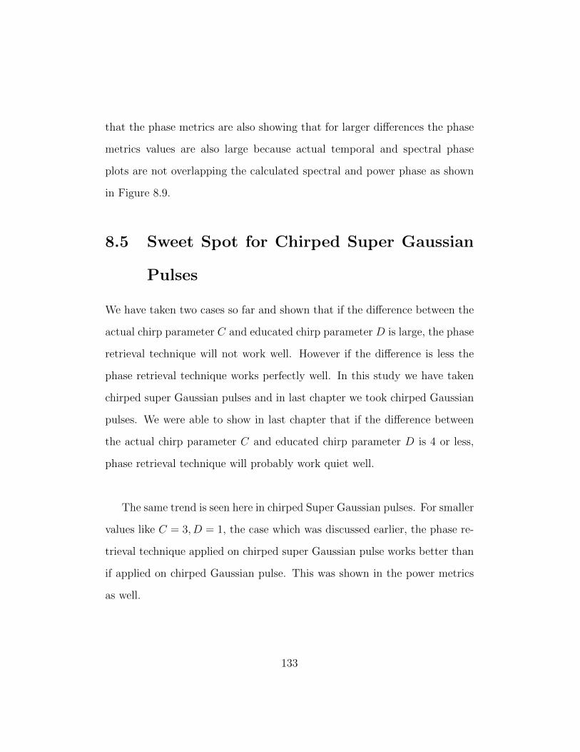
that the phase metrics are also showing that for larger differences the phase
metrics values are also large because actual temporal and spectral phase
plots are not overlapping the calculated spectral and power phase as shown
in Figure 8.9.
8.5 Sweet Spot for Chirped Super Gaussian
Pulses
We have taken two cases so far and shown that if the difference between the
actual chirp parameter C and educated chirp parameter D is large, the phase
retrieval technique will not work well. However if the difference is less the
phase retrieval technique works perfectly well. In this study we have taken
chirped super Gaussian pulses and in last chapter we took chirped Gaussian
pulses. We were able to show in last chapter that if the difference between
the actual chirp parameter C and educated chirp parameter D is 4 or less,
phase retrieval technique will probably work quiet well.
The same trend is seen here in chirped Super Gaussian pulses. For smaller
values like C = 3, D = 1, the case which was discussed earlier, the phase re-
trieval technique applied on chirped super Gaussian pulse works better than
if applied on chirped Gaussian pulse. This was shown in the power metrics
as well.
133
Figure 8.10: Power Metrics:Super Gaussian Pulse: C = 16, D = 1
Figure 8.10 shows relationship of difference between actual chirp param-
eter C and educated chirp parameter D and power metrics. if the difference
|C −D| is less than 5 then the power metrics show that the convergence of
phase retrieval technique on chirped Gaussian pulse is pretty good. However
there is an unusual spike at difference of |C −D| at 7. As the difference gets
larger the power metrics get large too showing that the converged temporal
power and spectral power are not overlapping actual temporal and spectral
power.
Figure 8.10 can be used as a reference when trying to choose for educated
134

guess parameter D. If by choosing some value of D we end up with a larger
power metric, that means the difference between the actual chirp parameter
of a chirped super Gaussian pulse and our educated chirp parameter is large.
Therefore we need to use a different D.
135
Bibliography
[1] C Dainty JR Fienup. Phase retrieval and image reconstruction for as-
tronomy. Image Recovery: Theory and Application, ed. byH. Stark,
Academic Press, San Diego, pages 231–275, 1987.
[2] J. R. Fienup. Reconstruction of an object from the modulus of its fourier
transform. Opt. Lett., 3(1):27–29, Jul 1978.
[3] J. R. Fienup. Phase retrieval algorithms: a comparison. Appl. Opt.,
21(15):2758–2769, Aug 1982.
[4] J. R. Fienup. Phase-retrieval algorithms for a complicated optical sys-
tem. Appl. Opt., 32(10):1737–1746, Apr 1993.
[5] J. R. Fienup, J. C. Marron, T. J. Schulz, and J. H. Seldin. Hubble space
telescope characterized by using phase-retrieval algorithms. Appl. Opt.,
32(10):1747–1767, Apr 1993.
[6] Manuel Guizar-Sicairos and James R Fienup. Image reconstruction by
phase retrieval with transverse translation diversity. In Optical Engi-
136
neering+ Applications, pages 70760A–70760A. International Society for
Optics and Photonics, 2008.
[7] H.A. Hauptman. The phase problem of x-ray crystallography.
Hauptman-Woodward Medical Research Institute, Inc., 1991.
[8] E. T. J. Nibbering, M. A. Franco, B. S. Prade, G. Grillon, J.-P. Cham-
baret, and A. Mysyrowicz. Spectral determination of the amplitude
and the phase of intense ultrashort optical pulses. J. Opt. Soc. Am. B,
13(2):317–329, Feb 1996.
[9] J. Peatross and A. Rundquist. Temporal decorrelation of short laser
pulses. J. Opt. Soc. Am. B, 15(1):216–222, Jan 1998.
[10] Andy Rundquist, Anatoly Efimov, and David H. Reitze. Pulse shaping
with the gerchberg-saxton algorithm. J. Opt. Soc. Am. B, 19(10):2468–
2478, Oct 2002.
137
Related Documents