` PHASE FIELD MODELING A REPORT SUBMITTED ON THE COMPLETION OF SUMMER INTERNSHIP AT BHABHA ATOMIC RESEARCH CENTRE . UNDER THE GUIDANCE OF: SUBMITTD BY: DR. ASHOK ARYA NITIN SINGH MATERIALS SCIENCE DIVISION 09MT3010 BHABHA ATOMIC RESEARCH CENTRE IIT KHARAGPUR MUMBAI

Phase Field Modeling
Oct 29, 2014
An introduction to phase filed modeling is being provided along with the methodology to solve few common problems in most general environment.
Welcome message from author
This document is posted to help you gain knowledge. Please leave a comment to let me know what you think about it! Share it to your friends and learn new things together.
Transcript
`
PHASE FIELD
MODELING A REPORT SUBMITTED ON THE COMPLETION OF SUMMER
INTERNSHIP AT BHABHA ATOMIC RESEARCH CENTRE .
UNDER THE GUIDANCE OF: SUBMITTD BY:
DR. ASHOK ARYA NITIN SINGH
MATERIALS SCIENCE DIVISION 09MT3010
BHABHA ATOMIC RESEARCH CENTRE IIT KHARAGPUR
MUMBAI
[Pick the date]
1
INTRODUCTION: The phase-field method has recently
emerged as a powerful computational approach to modeling and
predicting mesoscale morphological and microstructure evolution
in materials. It describes a microstructure using a set of conserved
and non conserved field variables (or order parameters) that are
continuous across the interfacial regions. The temporal and
spatial evolution of the field variables is governed by the Cahn-
Hilliard nonlinear diffusion equation and the Allen-Cahn
relaxation equation. With the fundamental thermodynamic and
kinetic information as the input, the phase-field method is able to
predict the evolution of arbitrary morphologies and complex
microstructures without explicitly tracking the positions of
interfaces.
1 - WHY PHASE FIELD MODELLING IS IMPORTANT
IN MATERIAL SCIENCE? The properties of most engineered materials have a connection
with their underlying microstructure. For example, the crystal
structure and impurity content of silicon will determine its band
structure and its subsequent quality of performance in modern
electronics. Most large-scale civil engineering applications demand
high-strength steels containing a mix of refined crystal grains and
a dispersion of hard and soft phases throughout their
microstructure. For aerospace and automotive applications, where
weight to strength ratios are a paramount issue, lighter alloys are
strengthened by precipitating second-phase particles within the
original grain structure. The combination of grain boundaries,
precipitated particles, and the combination of soft and hard
regions allow metals to be very hard and still have room for
ductile deformation. It is notable that the lengthening of span
bridges in the world can be directly linked to the development of
pearlitic steels. In general, the technological advance of societies
has often been linked to their ability to exploit and engineer new
materials and their properties.
In most of the above examples, as well as a plethora of
untold others, microstructures are developed during the process of
solidification, solid-state precipitation, and thermomechanical
processing. All these processes are governed by the fundamental
[Pick the date]
2
physics of free boundary dynamics and nonequilibrium phase
transformation kinetics. For example, in solidification and
recrystallization – both of which serve as a paradigm of a first-
order transformation – nucleation of crystal grains is followed by a
competitive growth of these grains under the drive to reduce the
overall free energy – bulk and surface – of the system, limited,
however, in their kinetics by the diffusion of heat and mass.
Thermodynamic driving forces can vary. For example,
solidification is driven by bulk free energy minimization, surface
energy and anisotropy. On the other hand, strain-induced
transformation must also incorporate elastic effects. These can
have profound effects on the morphologies and distribution of, for
example, second-phase precipitates during heat treatment of an
alloy.
The above raised arguments are quite sufficient to support
the cause of understanding and simulating the formation of
microstructure. Phase Field Modeling has emerged as a powerful
tool to simulate the evolution of microstructure which is much
easier than its predecessor („sharp interface approach‟) for such
work in terms of mathematics and its application. The following
section will make it much clearer.
1.2 - SHARP INTERFACE APPROACH:
In conventional modeling technique of for phase transformations
and microstructural evolution i.e the sharp interface approach,
the interfaces between different domains are considered to be
infinitely sharp, and a multi-domain structure is described by the
position of the interfacial boundaries. The kinetics of
microstructure formation is then modeled by a set of partial
differential equations that describe the release and diffusion of
heat, the transport of impurities, and the complex boundary
conditions that govern the thermodynamics at the interface for
each domain
. As a concrete example, in the solidification of a pure
material the advance of the solidification front is limited by the
diffusion of latent heat away from the solid–liquid interface, and
the ability of the interface to maintain two specific boundary
conditions; flux of heat toward one side of the interface is balanced
[Pick the date]
3
by an equivalent flux away from the other side, and the
temperature at the interface undergoes a curvature correction
known as the Gibbs–Thomson condition. These conditions are
mathematically expressed in the following sharp interface model,
commonly known as the Stefan problem:
∂T/∂t = ∇.(k.∇T/б.cp) = ∇.(α ∇T)
бLf Vn = ks∇T. n|sint - kL∇T. n|L
int (1)
Tint = Tm-(γTM/Lf)κ – (Vn/μ)
where T =T(x, t) denotes temperature, k thermal conductivity
(which assumes values ks and kL in the solid and liquid,
respectively), б the density of the solid and liquid, cp the specific
heat at constant pressure, α the thermal diffusion coefficient, Lf
the latent heat of fusion for solidification, γ the solid–liquid
surface energy, TM the melting temperature, κ the local solid
liquid interface curvature, Vn the local normal velocity of the
interface, and μ the local atomic interface mobility. Finally, the
subscript “int” refers to interface and the superscripts “S” and “L”
refer to evaluation at the interface on the solid and liquid side,
respectively.
Like solidification, there are other diffusion-limited phase
transformations whose interface properties can, on large enough
length scales, be described by specific sharp interface kinetics.
Most of them can be described by sharp interface equations
analogous to those in Equation 1. Such models – often referred to
as sharp interface models – operate on scales much larger than
the solid–liquid interface width, itself of atomic dimensions. As a
result, they incorporate all information from the atomic scale
through effective constants such as the capillary length, which
depend on surface energy, the kinetic attachment coefficient, and
thermal impurity diffusion coefficient.
1.3 - SHARP INTERFACE MODELS VS DIFFUSE INTERFACE
MODELS (MORE GENERALLY REFERRED TO AS PHASE
FIELD MODELS):
A limitation encountered in modeling free boundary problems is
that the appropriate sharp interface model is often not known for
[Pick the date]
4
many classes of phenomena. For example, the sharp interface
model for phase separation or particle coarsening, while easy to
formulate nominally , is unknown for the case when mobile
dislocations and their effect of domain coarsening are included. A
similar situation is encountered in the description of rapid
solidification when solute trapping and drag are relevant. There
are several sharp interface descriptions of this phenomenon, each
differing in the way they treat the phenomenological drag
parameters and trapping coefficients and lateral diffusion along
the interface.
Another drawback associated with sharp interface
models is that their numerical simulation also turns out to be
extremely difficult. The most challenging aspect is the complex
interactions between topologically complex interfaces that
undergo merging and pinch-off during the course of a phase
transformation. Such situations are often addressed by applying
somewhat arbitrary criteria for describing when interface merging
or pinch-off occurs and by manually adjusting the interface
topology. It is worth noting that numerical codes for sharp
interface models are very lengthy and complex, particularly in 3D.
Along with these two drawbacks of sharp
interface models, one would not be able to completely appreciate
the diffuse interface approach if the most important advantage of
the later over former is not mentioned here. Main advantage
gained by using phase-field method to model phase transitions,
compared to the sharp-interface method, is that the explicit
tracking of the moving surface, the liquid and solid interface, is
completely avoided. Instead, the phase of each point in the
simulated volume is computed at each time step. In classical
formulation the basic equations have to be written for each
medium and the interface boundary conditions must be explicitly
tracked. In diffuse-interface theory the basic equations, with
supplementary phase field terms, are deduced from a free energy
functional for the whole system and interface conditions do not
occur. In fact, they are replaced by a partial differential equation
for the phase field.
[Pick the date]
5
2 – DETAILS OF PHASE FIELD MODELLING: As already mentioned, the phase field method has proved to be
extremely powerful in the visualization of the development of
microstructure without having to track the evolution of individual
interfaces, as is the case with sharp interface models. The method,
within the framework of irreversible thermodynamics, also allows
many physical phenomena to be treated simultaneously.
The primary purpose of this section is to present the general
concepts underlying the phase field modeling.
Imagine the growth of a
precipitate which is isolated from the matrix by an interface.
There are three distinct entities to consider: the precipitate,
matrix and interface. The interface can be described as an
evolving surface whose motion is controlled according to the
boundary conditions consistent with the mechanism of
transformation. The interface in this mathematical description is
simply a two dimensional surface; it is said to be a sharp interface
which is associated with an interfacial energy σ per unit area.
In the phase field method, the state of the entire
microstructure is represented continuously by a single variable
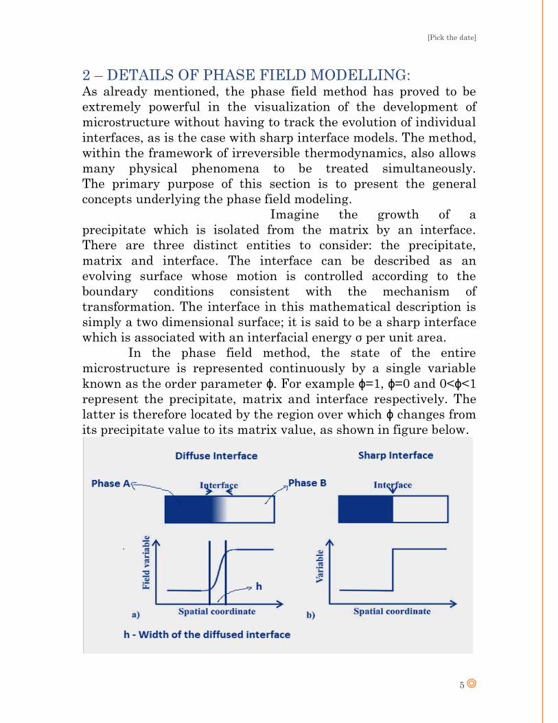
known as the order parameter ϕ. For example ϕ=1, ϕ=0 and 0<ϕ<1
represent the precipitate, matrix and interface respectively. The
latter is therefore located by the region over which ϕ changes from
its precipitate value to its matrix value, as shown in figure below.
[Pick the date]
6
The range over which it changes is the width of the interface. The
set of values of the order parameter over the whole volume is the
phase field. The total free energy G of the volume is then
described in terms of the order parameter and its gradients, and
the rate at which the structure evolves with time is set in the
context of irreversible thermodynamics, and depends on how G
varies with ϕ. It is the gradients in thermodynamic variables that
drive the evolution of structure.
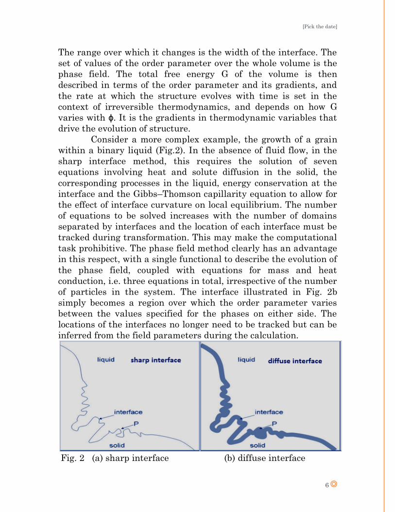
Consider a more complex example, the growth of a grain
within a binary liquid (Fig.2). In the absence of fluid flow, in the
sharp interface method, this requires the solution of seven
equations involving heat and solute diffusion in the solid, the
corresponding processes in the liquid, energy conservation at the
interface and the Gibbs–Thomson capillarity equation to allow for
the effect of interface curvature on local equilibrium. The number
of equations to be solved increases with the number of domains
separated by interfaces and the location of each interface must be
tracked during transformation. This may make the computational
task prohibitive. The phase field method clearly has an advantage
in this respect, with a single functional to describe the evolution of
the phase field, coupled with equations for mass and heat
conduction, i.e. three equations in total, irrespective of the number
of particles in the system. The interface illustrated in Fig. 2b
simply becomes a region over which the order parameter varies
between the values specified for the phases on either side. The
locations of the interfaces no longer need to be tracked but can be
inferred from the field parameters during the calculation.
Fig. 2 (a) sharp interface (b) diffuse interface
[Pick the date]
7
Notice that the interface in Fig. 2b is drawn as a region with finite
width, because it is defined by a smooth variation in ϕ between ϕ=
0(solid) and ϕ=1(liquid). The order parameter does not change
discontinuously during the traverse from the solid to the liquid.
The position of the interface is fixed by the surface where ϕ=0.5.
2.1 - ORDER PARAMETER:
The order parameter in phase field modeling is a function
of space and time which may or may not have macroscopic
physical interpretations. For two-phase materials, ϕ is typically
set to 0 and 1 for the individual phases, and the interface is the
domain where 0<ϕ<1. For the general case of N phases present in
a matrix, there will be a corresponding number of phase field
order parameters ϕi with i=1 to N. ϕi=1 then represents the
domain where phase i exists, ϕi=0 where it is absent and 0<ϕi<1
its bounding interfaces. Suppose that the matrix is represented by
ϕo then it is necessary that at any location:
N
Σ ϕi = 1
i=0
It follows that the interface between phases 1 and 2, where 0<ϕ1<1
and 0<ϕ2<1 is given by ϕ1+ ϕ2 =1; similarly, for a triple junction
between three phases where 0<ϕi<1 for i=1,2,3, the junction is the
domain where ϕ1+ ϕ2+ ϕ3 = 1.
The order parameters in phase field modeling can be the
either of two types:
Conserved Order Parameters – Conserved quantities as quite
clearly decipherable, are the ones which remain unchanged during
the process to be studied. Example can be the concentration of an
element or alloy undergoing solidification, because the average
concentration is never going to change. The change in conserved
order parameters with time is governed by Cahn-Hilliard
equation.
Non-conserved Order Parameters – Non-conserved quantities
are the ones that change during a process. Example can be spin
or crystalline order. The change in non-conserved order
parameters with time is governed by Cahn-Allen equation.
[Pick the date]
8
2.2 – GOVERNING EQUATIONS AND MATHEMATICS OF
PHASE FIELD MODELLING:
“Derivations of the important expressions are given in full, on the
premise that it is easier for a reader to skip a step than it is for
another to bridge the algebraic gap between it is easily shown that
and the ensuing equation” – J.E Hilliard (on the mathematics of
their phase field model for spinodal decomposition)
As a first requirement for any problem to be modeled by phase
field modeling, a free energy functional (for isothermal cases
and for non-isothermal cases free entropy functional) has to
be defined as a function of order parameter. The general
expression of a free energy functional is shown below:
F = ʃv [f (ϕ, c, T) + (Ɛ2c/2)*| ∇c|2 + (Ɛ2
ϕ/2)*| ∇ϕ|2] dv (2)
The first term in the left hand side of the equation is free energy
density of the bulk phase as a function of concentration, order
parameter and temperature. The second and the third term
denote the energy of the interface. The second term denotes the
energy due to the gradient present in the concentration and the
third term denotes the energy due to the gradient present in the
order parameter.
After doing a little bit of mathematics (which is intentionally
ignored here, considering the point that only the application of
these equations shall be sufficient at undergraduate level study),
one arrives at two kinds of equation. The first one is for conserved
order parameters and the second one is for non-conserved order
parameters.
Cahn-Hilliard Equation – Cahn-Hilliard equation gives the rate
of change of conserved order parameter with time.
∂ ϕ /∂t = M.∇2[∂f/∂ϕ - Ɛ2ϕ ∇2ϕ] (3)
The above equation is for constant (position-independent) mobility
M. ϕ is order parameter, ∇ is divergence, f is free energy of the
bulk, Ɛϕ is gradient energy coefficient. As one can quite clearly
notice that Cahn-Hilliard equation is nothing but modified form of
Fick‟s second law for transient diffusion.
[Pick the date]
9
Cahn-Allen Equation - Cahn-Allen equation gives the rate of
change of non-conserved order parameter with time.
∂ϕ/∂t = -M [∂f/∂ϕ – Ɛ2ϕ ∇2ϕ] (4)
Cahn-Allen equation is also known as time-dependent Ginsburg-
Landau equation.
Note: While deriving the Cahn-Hilliard and Cahn-Allen equation,
an important expression ∂ϕ/∂t = M*∂F/∂ϕ was used, which clearly
does makes sense because the change in free energy functional
with respect to change in order parameter ϕ, must be in some
relation with change in order parameter ϕ with respect to time.
2.3 – PSEUDO ALGORITHM TO MODEL A PROCESS VIA
PHASE FIELD MODELING:
The “diffuse interface‟ idea can be extended to almost all systems
with an evolution of microstructure or interfacial boundary
involved in it. Here is the Pseudo algorithm to approach a
problem:
Describe the microstructure using a suitable set of field
variables (commonly referred as order parameters), some are
conserved variables and others are non-conserved.
Write the energy of a configuration consistent with the
system‟s thermodynamics. It will have both bulk and
gradient energy terms, similar to as equation (2)
Write the evolution equations: Cahn-Hilliard equation for
conserved variables, and Cahn-Allen equation for non-
conserved variables.
Discretize the evolution equations via a suitable scheme (a
variety of schemes can be found in the literature, each
having their own advantages over others) to solve it
numerically.
Provide the system inputs as well as spacial and time
information and then numerically march in time in order to
evolve the order parameters.
Hope (pray?) that your model will behave nicely!

[Pick the date]
10
3 – EXAMPLES: As already explained, a diffuse interface approach is very much
capable to model almost any kind of problem in the field of
material science. The most common problems that are solved are:
Spinodal decomposition.
Isothermal and non-isothermal solidification.
Disorder – order phase transformation.
Grain growth during recrystallization.
Dislocation dynamics.
Dendritic growth.
A problem involving a combination of above mentioned and many
a others to count.
In the present report, three kinds of problem i.e Spinodal
Decomposition, Isotermal Solidification for pure substance
and Dendritic Growth for pure substance are studied, their
theory and a detailed method to solve them via phase field
modeling is presented
3.1 – SPINODAL DECOMPOSITION:
Spinodal decomposition is a mechanism by which a solution of two
or more components can separate into distinct regions (or phases)
with distinctly different chemical compositions and physical
properties. This mechanism differs from classical nucleation in
that phase separation due to spinodal decomposition is much more
subtle, and occurs uniformly throughout the material and not just
at discrete nucleation sites.
Spinodal decomposition is of interest for two
primary reasons. In the first place, it is one of the few phase
transformations in solids for which there is any plausible
quantitative theory. The reason for this is the inherent simplicity
of the reaction. Since there is no thermodynamic barrier to the
reaction inside of the spinodal region, the decomposition is
determined solely by diffusion. Thus, it can be treated purely as a
diffusional problem.
From a more practical standpoint, spinodal decomposition
provides a means of producing a very finely dispersed
microstructure that can significantly enhance the physical
properties of the material.
[Pick the date]
11
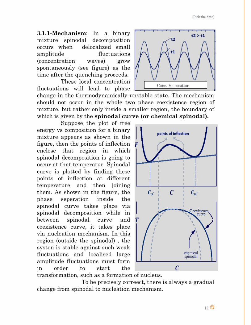
3.1.1-Mechanism: In a binary
mixture spinodal decomposition
occurs when delocalized small
amplitude fluctuations
(concentration waves) grow
spontaneously (see figure) as the
time after the quenching proceeds.
These local concentration
fluctuations will lead to phase
change in the thermodynamically unstable state. The mechanism
should not occur in the whole two phase coexistence region of
mixture, but rather only inside a smaller region, the boundary of
which is given by the spinodal curve (or chemical spinodal).
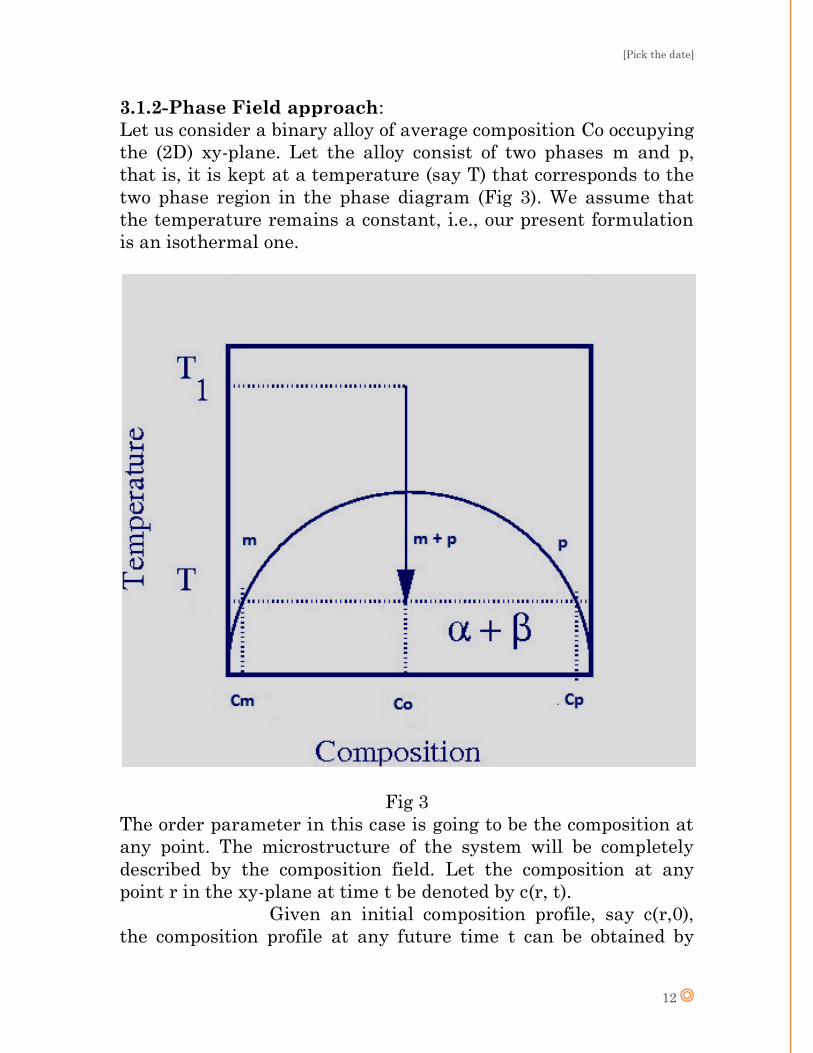
Suppose the plot of free
energy vs composition for a binary
mixture appears as shown in the
figure, then the points of inflection
enclose that region in which
spinodal decomposition is going to
occur at that temperatur. Spinodal
curve is plotted by finding these
points of inflection at different
temperature and then joining
them. As shown in the figure, the
phase seperation inside the
spinodal curve takes place via
spinodal decomposition while in
between spinodal curve and
coexistence curve, it takes place
via nucleation mechanism. In this
region (outside the spinodal) , the
systen is stable against such weak
fluctuations and localised large
amplitude fluctuations must form
in order to start the
transformation, such as a formation of nucleus.
To be precisely correect, there is always a gradual
change from spinodal to nucleation mechanism.
Conc. Vs position
[Pick the date]
12
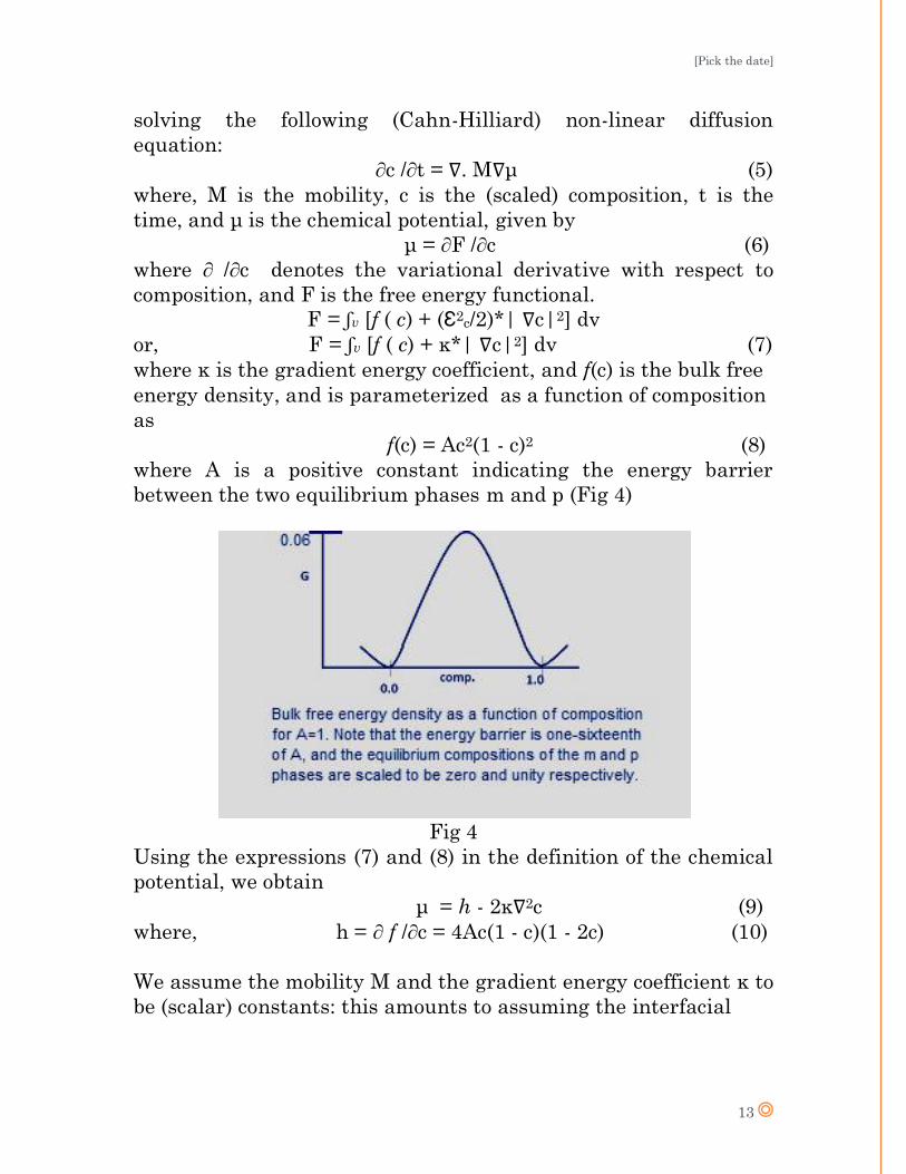
3.1.2-Phase Field approach:
Let us consider a binary alloy of average composition Co occupying
the (2D) xy-plane. Let the alloy consist of two phases m and p,
that is, it is kept at a temperature (say T) that corresponds to the
two phase region in the phase diagram (Fig 3). We assume that
the temperature remains a constant, i.e., our present formulation
is an isothermal one.
Fig 3
The order parameter in this case is going to be the composition at
any point. The microstructure of the system will be completely
described by the composition field. Let the composition at any
point r in the xy-plane at time t be denoted by c(r, t).
Given an initial composition profile, say c(r,0),
the composition profile at any future time t can be obtained by
[Pick the date]
13
solving the following (Cahn-Hilliard) non-linear diffusion
equation:
∂c /∂t = ∇. M∇μ (5)
where, M is the mobility, c is the (scaled) composition, t is the
time, and μ is the chemical potential, given by
μ = ∂F /∂c (6)
where ∂ /∂c denotes the variational derivative with respect to
composition, and F is the free energy functional.
F = ʃv [f ( c) + (Ɛ2c/2)*| ∇c|2] dv
or, F = ʃv [f ( c) + κ*| ∇c|2] dv (7)
where κ is the gradient energy coefficient, and f(c) is the bulk free
energy density, and is parameterized as a function of composition
as
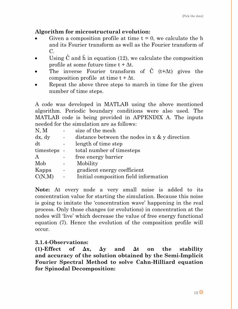
f(c) = Ac2(1 - c)2 (8)
where A is a positive constant indicating the energy barrier
between the two equilibrium phases m and p (Fig 4)
Fig 4
Using the expressions (7) and (8) in the definition of the chemical
potential, we obtain
μ = h - 2κ∇2c (9)
where, h = ∂ f /∂c = 4Ac(1 - c)(1 - 2c) (10)
We assume the mobility M and the gradient energy coefficient κ to
be (scalar) constants: this amounts to assuming the interfacial

[Pick the date]
14
energies and the diffusivities to be isotropic.
Using the Equation (9) above, and the fact that M is a constant,
we obtain the Cahn-Hilliard equation as follows:
∂c /∂t = M∇2(h - 2κ∇2c) (11)
3.1.3-Numerical Method to solve equation (11):
Since Cahn-Hilliard equation is nonlinear, it can only be solved
numerically through discretization in space and time. Due to its
simplicity and small memory requirement, most of the phase-field
simulations in the literature employed the explicit forward Euler
method in time and finite-difference in space. To maintain the
stability and to achieve high accuracy for the solutions, the time
step and spatial grid size have to be very small, which seriously
limits the system size and time duration of a simulation. The
ability to performing reliable long-time simulation
is critical in the fundamental understanding of the scaling
behavior of morphological pattern evolution.
In this report, we implement an accurate and
efficient semi-implicit Fourier-spectral method suggested by
L.Q.Chen, J.Shen for solving the phase-field equations. For the
time variable semi-implicit scheme is being employed. Thanks to
the exponential convergence of the Fourier-spectral discretization,
it requires a significantly smaller number of grid points to resolve
the solution to within a prescribed accuracy, say 1%. Moreover,
the semi-implicit Fourier spectral method is easy to implement
and can be extended for systems with position-dependent mobility.
Equation (11) is first non-dimensionalised and is then
discretised by employing Semi-Implicit Fourier-Spectral Method.
The discretised equation is:
Ĉ(k, t+Δt) = Ĉ(k, t) – ΔtMk2ĥ(k,t) (12) 1 + 2ΔtMk4 κ
In the above equation Ĉ and ĥ represent the fourier transform of
composition field and h field, where h is given by equation (10). k
= (k1, k2) is a vector in the Fourier space, k = (k12+k22)1/2 is the
magnitude of k. Other symbols have their usual meanings.
[Pick the date]
15
Algorithm for microstructural evolution:
Given a composition profile at time t = 0, we calculate the h
and its Fourier transform as well as the Fourier transform of
C.
Using Ĉ and ĥ in equation (12), we calculate the composition
profile at some future time t + Δt.
The inverse Fourier transform of Ĉ (t+Δt) gives the
composition profile at time t + Δt.
Repeat the above three steps to march in time for the given
number of time steps.
A code was developed in MATLAB using the above mentioned
algorithm. Periodic boundary conditions were also used. The
MATLAB code is being provided in APPENDIX A. The inputs
needed for the simulation are as follows:
N, M - size of the mesh
dx, dy - distance between the nodes in x & y direction
dt - length of time step
timesteps - total number of timesteps
A - free energy barrier
Mob - Mobility
Kappa - gradient energy coefficient
C(N,M) - Initial composition field information
Note: At every node a very small noise is added to its
concentration value for starting the simulation. Because this noise
is going to imitate the „concentration wave‟ happening in the real
process. Only those changes (or evolutions) in concentration at the
nodes will „live‟ which decrease the value of free energy functional
equation (7). Hence the evolution of the composition profile will
occur.
3.1.4-Observations:
(1)-Effect of Δx, Δy and Δt on the stability
and accuracy of the solution obtained by the Semi-Implicit
Fourier Spectral Method to solve Cahn-Hilliard equation
for Spinodal Decomposition:
[Pick the date]
16
All the results correspond to a double well free energy potential
function with minima at 0 and 1. And the value of initial
composition i.e c_0 = 0.5.
Effect of Δx and Δy with Δt = 1.0 - Keeping all the
thermodynamic parameters i.e A, kappa, mobility equal to one
and a 256x256 mesh size, it was observed that stable solution was
obtained in the range of Δx = Δy = [0.45, 2.5]. The accuracy of
solution increased as the value was increased from 1.0. The
increase in accuracy can be attributed to the fact that all the
numerical methods to solve a Partial Differential Equation suffer
inaccuracy and anomaly when the value of Δt is larger than Δx ( or
Δy) beyond a certain value.
Effect of Δt with and Δy = 1.0 - Keeping all the
thermodynamic parameters i.e A, kappa, mobility equal to one
and a 256x256 mesh size, it was observed that stable solution was
obtained with Δt as large as 6.0 for the problem being examined.
The accuracy of the solution was of course better with smaller
value of Δt. None of the earlier proposed method to solve the
corresponding discretized equations could be able to handle such a
large value of time step. This is surely one of the major
advantages of Semi-Implicit Fourier Spectral Method where the
emphasis may be on quantitative analysis rather than precise
accuracy.
However, to be on the safer side for all the discussions that
follow the values chosen are Δx = Δy = 1.0, Δt = 2.5.
(2)- Effect of Initial Concentration on the solvability of
Cahn-Hilliard equation for Spinodal Decomposition via
Semi-Implicit Fourier Spectral method for a double free
energy well potential function:
All the results correspond to a double well free energy potential
function with minima at 0 and 1.
When all the thermodynamic parameters were set to one,
the composition segregation occurred perfectly fine for initial
concentration value c_0 in the range (0.3, 0.7).
[Pick the date]
17
However, when the initial composition value was chosen in
the range of (0, 0.3] or [0.7, 1), the composition segregation did not
occur and the concentration values at all points moved to the
nearest free energy double well potential minima in each case.
One possible explanation to this observation
can be that when the value of c_0 is too small (or too large) to
jump the free energy barrier, the composition segregation becomes
impossible to be achieved. As a solution to this problem, the value
of A was increased. It was observed that below c_0 = 0.3, value of
A=1.3(or greater) was able to show composition segregation.
However, the value of A has to be progressively increased as we
approach c_0 nearer to 0.0. The same holds true when the value of
c_0 is greater than or equal to 0.7
For all the discussions that follow, c_0 = 0.5 will be used in
computations.
(3) Effect of noise strength on the microstructure evolution
during Spinodal Decomposition:
Why the noise was introduced into the system?
Spinodal Decomposition occurs when in a thermodynamically
unstable initial state, long wavelength small amplitude stastical
fluctuations grow spontaneously in amplitude as time proceeds. To
simulate, these „concentration waves‟ (or simply concentration
fluctuations), randomness about average composition is
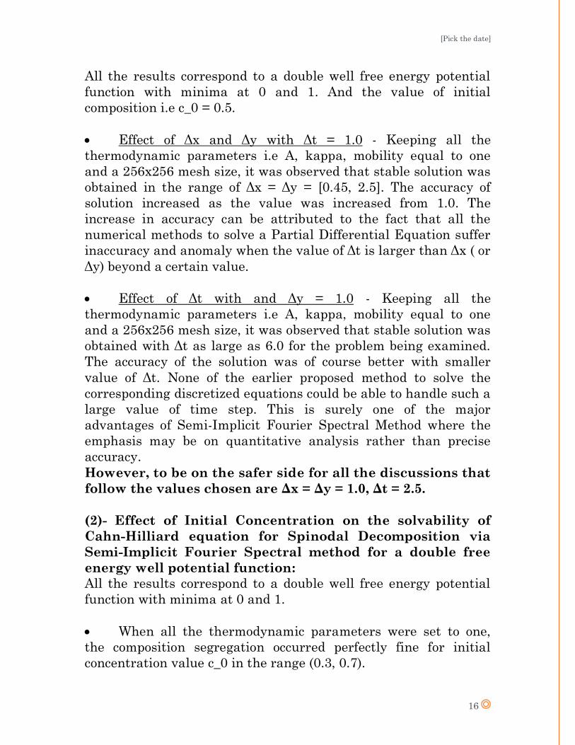
introduced by imparting a small noise to the system.
Case1 - Noise = 0.5*10-1 Case2 - Noise = 0.5* 10-2
t = 2.5 t = 2.5
[Pick the date]
18
t = 62.5 t = 62.5
t = 150 t = 150
Conclusions drawn from the above results:
Before we proceed, we must make a point clear that a noise value
of 0.5*10-1 is quite large and is rarely experienced by any system,
however just for the sake of comparison we have chosen it against
the one that is having far more possibility of occurring.
t = 2.5 - As the value of noise in increased, after the first time
step, larger concentration segregation is observed in Case1. In
Case1 the range of concentration was [0.4854, 0.5149], whereas in
the Case2 the range was [0.498, 0.501].
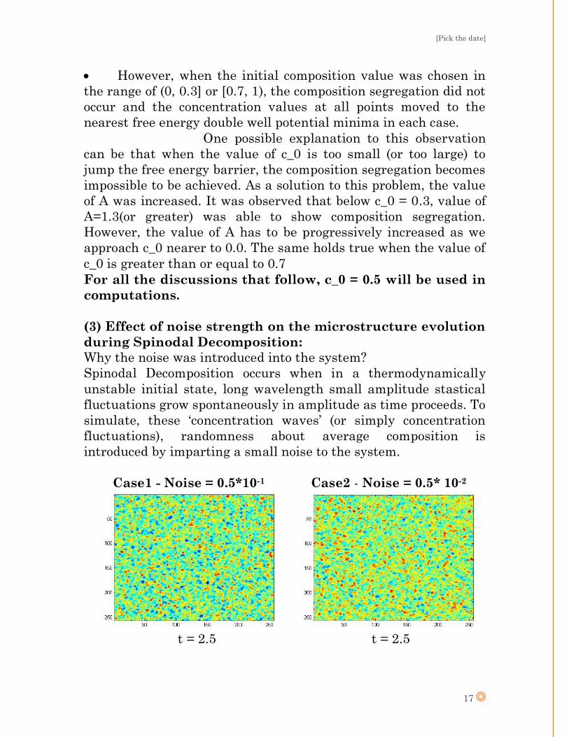
t = 62.5 – The concentration segregation was greater in Case1
than Case2 as it can be clearly seen in the images shown above as
well. The area covered by the diffuse interface was also lesser for
the Case1 then Case2.
[Pick the date]
19
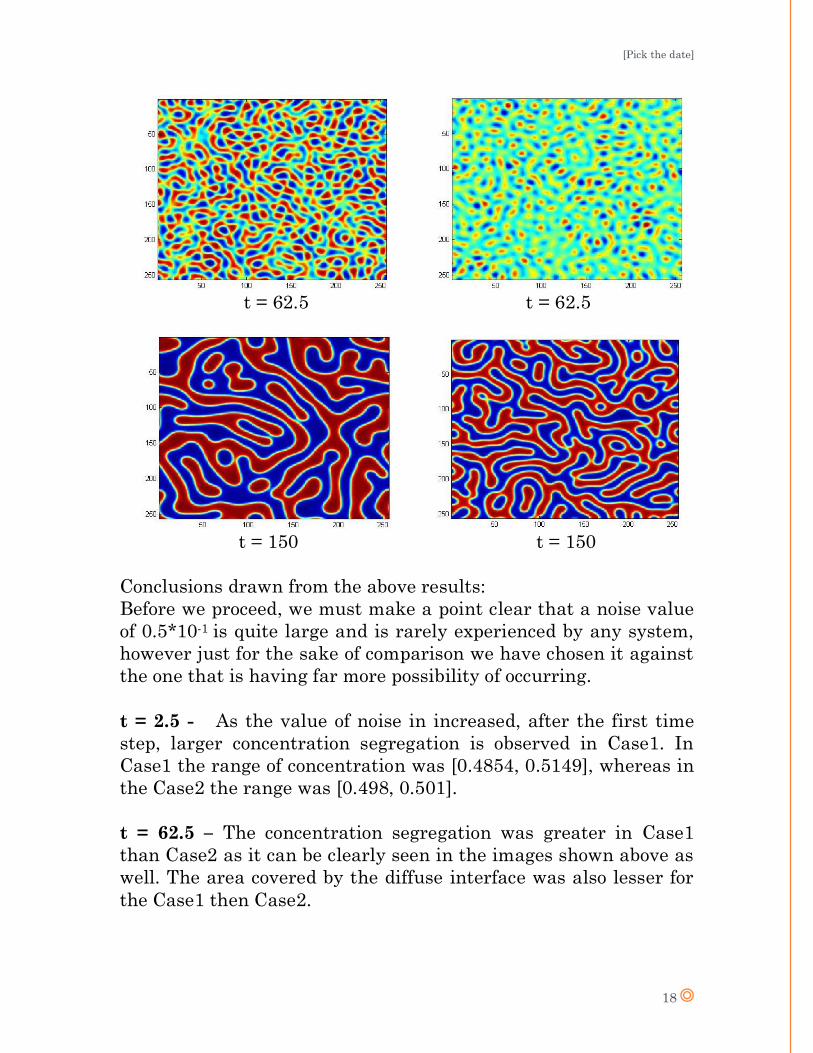
t = 450 – At this time, the shape and size of the region occupied by
two phases in Case1 became more or less stable and the system
seemed to have attained the final state with well segregated
regions. However in Case2, the decomposition was not stabilized
and the coarsening of the regions would have continued had the
system been allowed more time to stand.
From the above discussion, few conclusions that can be
made are that with larger noise the segregation becomes easy and
that system attains equilibrium state relatively quickly. Moreover
at any time, the area covered by the diffuse interface in the
microstructure is lesser. For the proceeding discussions, the
value of noise strength will be 0.5*10-2 unless otherwise
stated.
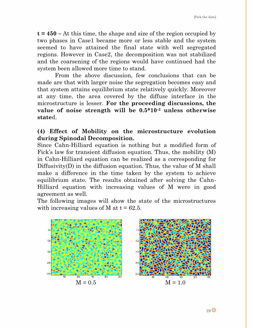
(4) Effect of Mobility on the microstructure evolution
during Spinodal Decomposition.
Since Cahn-Hilliard equation is nothing but a modified form of
Fick‟s law for transient diffusion equation. Thus, the mobility (M)
in Cahn-Hilliard equation can be realized as a corresponding for
Diffusivity(D) in the diffusion equation. Thus, the value of M shall
make a difference in the time taken by the system to achieve
equilibrium state. The results obtained after solving the Cahn-
Hilliard equation with increasing values of M were in good
agreement as well.
The following images will show the state of the microstructures
with increasing values of M at t = 62.5.
M = 0.5 M = 1.0
[Pick the date]
20
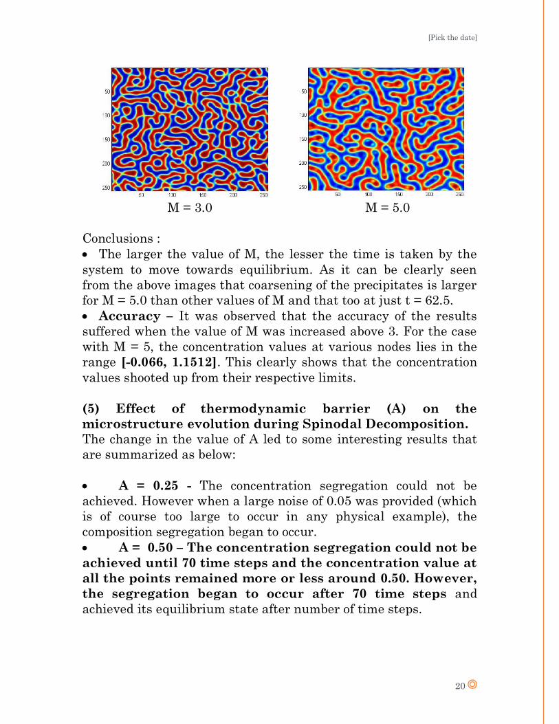
M = 3.0 M = 5.0
Conclusions :
The larger the value of M, the lesser the time is taken by the
system to move towards equilibrium. As it can be clearly seen
from the above images that coarsening of the precipitates is larger
for M = 5.0 than other values of M and that too at just t = 62.5.
Accuracy – It was observed that the accuracy of the results
suffered when the value of M was increased above 3. For the case
with M = 5, the concentration values at various nodes lies in the
range [-0.066, 1.1512]. This clearly shows that the concentration
values shooted up from their respective limits.
(5) Effect of thermodynamic barrier (A) on the
microstructure evolution during Spinodal Decomposition.
The change in the value of A led to some interesting results that
are summarized as below:
A = 0.25 - The concentration segregation could not be
achieved. However when a large noise of 0.05 was provided (which
is of course too large to occur in any physical example), the
composition segregation began to occur.
A = 0.50 – The concentration segregation could not be
achieved until 70 time steps and the concentration value at
all the points remained more or less around 0.50. However,
the segregation began to occur after 70 time steps and
achieved its equilibrium state after number of time steps.
[Pick the date]
21
A = 1.0 - The segregation in this case occurred just fine
right from the start and achieved equilibrium after around 300
time steps.
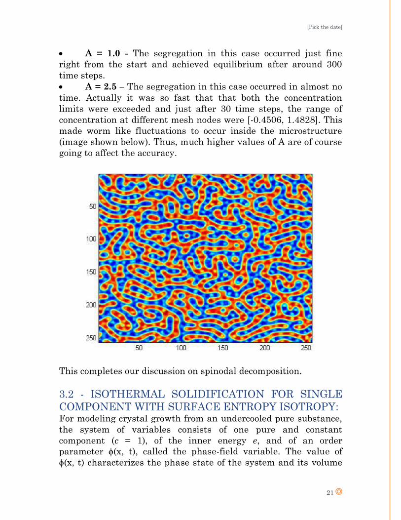
A = 2.5 – The segregation in this case occurred in almost no
time. Actually it was so fast that that both the concentration
limits were exceeded and just after 30 time steps, the range of
concentration at different mesh nodes were [-0.4506, 1.4828]. This
made worm like fluctuations to occur inside the microstructure
(image shown below). Thus, much higher values of A are of course
going to affect the accuracy.
This completes our discussion on spinodal decomposition.
3.2 - ISOTHERMAL SOLIDIFICATION FOR SINGLE
COMPONENT WITH SURFACE ENTROPY ISOTROPY: For modeling crystal growth from an undercooled pure substance,
the system of variables consists of one pure and constant
component (c = 1), of the inner energy e, and of an order
parameter ϕ(x, t), called the phase-field variable. The value of
ϕ(x, t) characterizes the phase state of the system and its volume
[Pick the date]
22
fraction in space at time t. In contrast to classical sharp interface
models, the interfaces are represented by thin diffuse regions in
which ϕ(x, t) smoothly varies between the values of φ associated
with the adjoining bulk phases. For a solid–liquid phase system, a
phase-field model may be scaled such that ϕ(x, t) = 1 characterizes
the region of the solid phase and ϕ(x, t) = 0 the region of the liquid
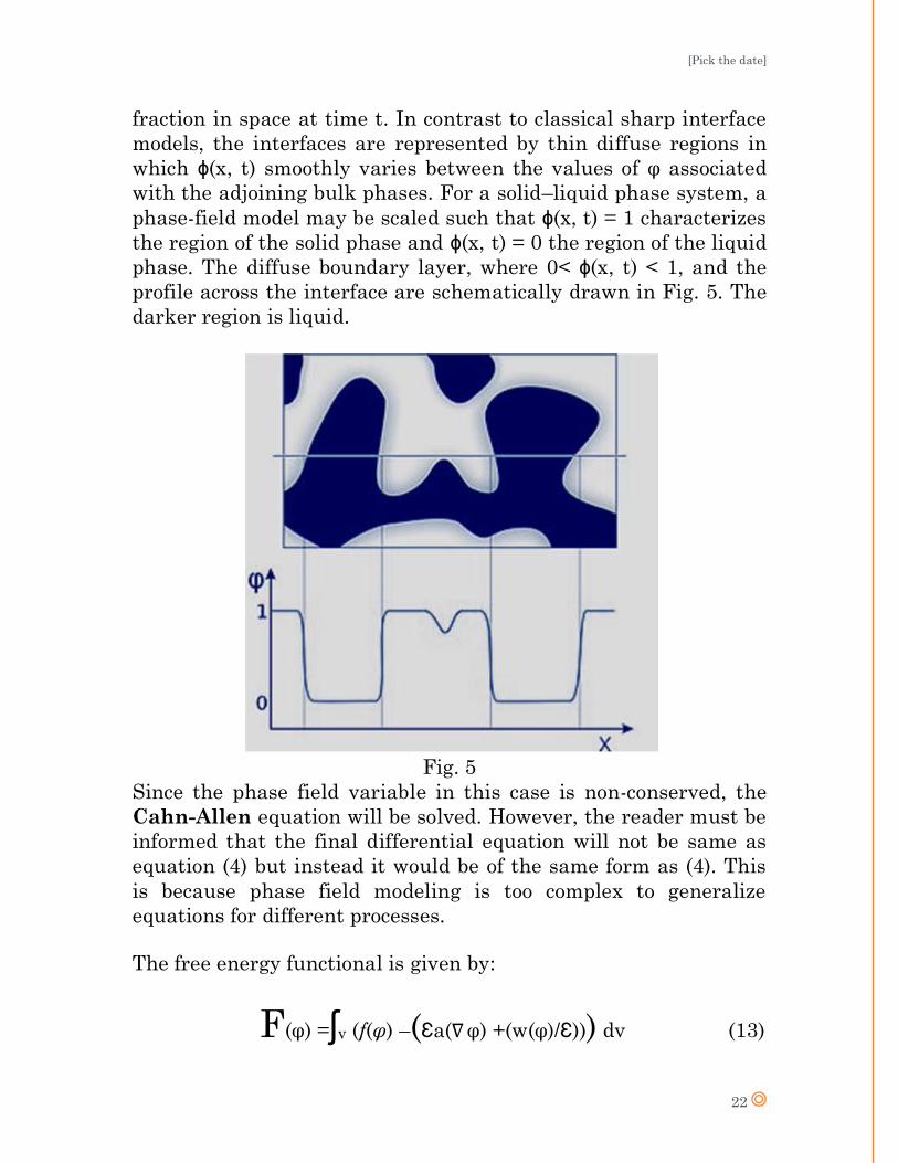
phase. The diffuse boundary layer, where 0< ϕ(x, t) < 1, and the
profile across the interface are schematically drawn in Fig. 5. The
darker region is liquid.
Fig. 5
Since the phase field variable in this case is non-conserved, the
Cahn-Allen equation will be solved. However, the reader must be
informed that the final differential equation will not be same as
equation (4) but instead it would be of the same form as (4). This
is because phase field modeling is too complex to generalize
equations for different processes.
The free energy functional is given by:
F(φ) =ʃv (f(φ) –(Ɛa(∇φ) +(w(φ)/Ɛ))) dv (13)
[Pick the date]
23
This equation is similar to the free energy functional shown
previously. The second term in the integral (enclosed in the
brackets) reflects the thermodynamics of the interface Ɛ is a small
length scale parameter related to the thickness of the diffuse
interface.
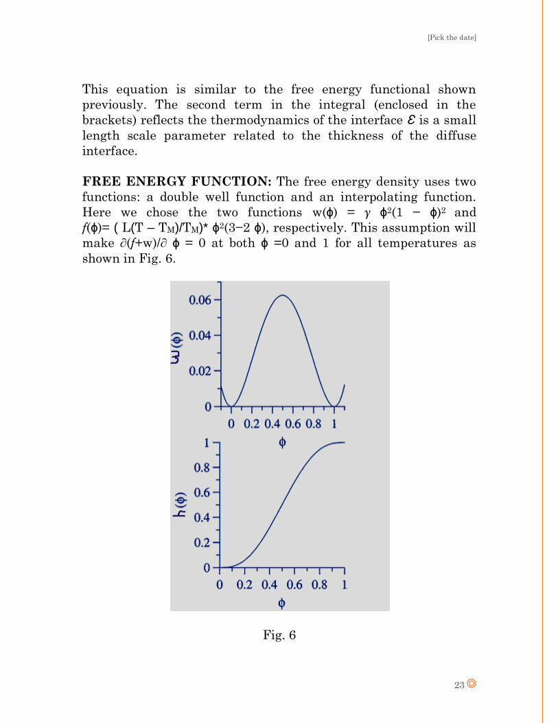
FREE ENERGY FUNCTION: The free energy density uses two
functions: a double well function and an interpolating function.
Here we chose the two functions w(ϕ) = γ ϕ2(1 − ϕ)2 and
f(ϕ)= ( L(T – TM)/TM)* ϕ2(3−2 ϕ), respectively. This assumption will
make ∂(f+w)/∂ ϕ = 0 at both ϕ =0 and 1 for all temperatures as
shown in Fig. 6.
Fig. 6
[Pick the date]
24
After applying the equation for the energy conservation, a phase
field equation Ɛτ∂ϕ/∂t = M*∂F/∂ϕ (where τ is kinetic mobility)
and a little bit of mathematics, the details of which are
intentionally avoided here, one arrives at the final partial
differential equation for the evolution of the phase field variable ϕ.
Ɛτ∂ϕ/∂t = ε∇ · a,∇ϕ(∇ϕ) - w,ϕ(ϕ)/Ɛ - f,ϕ(T,ϕ)/T (14)
where a,∇ϕ, w,ϕ, and f, ϕ denote the partial derivative with respect
to ∇ ϕ and ϕ, respectively.
f(T,ϕ) =( L(T – TM)/TM)* ϕ2(3 − 2ϕ) bulk free energy density
w(ϕ) = γ ϕ2(1 − ϕ)2 double well potential
a(∇ϕ) = γ ac2 (∇ ϕ)|∇ ϕ|2 gradient entropy density
where TM is the melting temperature and γ defines the surface
entropy density of the solid– liquid interface.
For the system of two phases, the gradient entropy
density reads a(∇ϕ) = γ|∇ϕ|2. The double well potential is w(ϕ) = γ
ϕ2(1 − ϕ)2. And f(T,ϕ) =m*ϕ2(3 − 2ϕ), where m is a constant bulk
energy density related to the driving force of the process, for
example, to the isothermal undercooling ΔT, for example, m =
m(ΔT). By utilizing the phase field equation and by inserting the
values of above mentioned term in equation (14), the modified
form of the partial differential equation becomes:
τƐ∂tϕ = Ɛ(2 γ) Δϕ − (18 γ (2ϕ3 − 3ϕ2 + ϕ)/Ɛ) − 6mϕ(1 −ϕ) (15)
Δϕ is the laplacian of the ϕ matrix.
3.2.1 – Numerical method to solve equation (15):
The most straightforward discretization of finite differences with
an explicit time marching scheme is used here by writing the
phase-field equation (15) in discrete form and by defining suitable
boundary conditions.
ϕi,jn+1 = ϕi,j +∂t/τ{2γ((ϕi+1,jn-2ϕi,j
n + ϕi-1,jn)/∂x2 + (ϕi,j+1
n- 2ϕi,jn+ ϕi,j1
n)/∂y2)
- A*18γ/Ɛ2(2(ϕi,jn)3-3)( ϕi,j
n)2+ ϕi,jn) – B*6m/Ɛ(ϕi,j
n(1- ϕi,jn))} (16)
[Pick the date]
25
Here, A,B ∈ {0, 1} are introduced in order to switch on or off the
corresponding terms in the phase-field equation for our later case
study. Two types of boundary conditions are used in the
simulation.
Periodic boundary condition: A periodic boundary condition
mimics an infinite domain size with a periodicity in the structure.
The values of the boundary are set to the value of the neighboring
cell from the opposite side of the domain.
ϕ1,j = ϕNx-1,j , ϕNx,j = ϕ2,j with j = 1, . . . , Ny
ϕi,1 = ϕi,Ny-1 , ϕi,Ny = ϕi,2 with 1 = 1, . . . , Nx
Neumann Boundary condition: The component of ∇ϕ normal to
the domain boundary should be zero. In our rectangular domain,
this can be realized by copying the ϕ value of the neighboring
(interior) cell to the boundary cell:
ϕ1,j = ϕ2,j , ϕNx,j = ϕNx-1,j with j = 1, . . . , Ny
ϕi,1 = ϕi,2 , ϕi,Ny = ϕi,Ny-1 with 1 = 1, . . . , Nx
Stability Condition: To ensure the stability of the explicit
numerical method and to avoid generating oscillations, the
following condition for the time step ∂t depending on the spatial
discretizations ∂x and ∂y must be fulfilled:
∂t < (1/4γ)*(1/∂x2 + 1/∂y2)-1
A code in Matlab was developed to evolve the phase field variable
using equation (16) and suitable boundary conditions. The code is
being provided in APPENDIX B. The inputs needed for the
simulation are as follows:
N, M - size of the mesh
dx, dy - distance between the nodes in x & y direction
dt - length of time step
timesteps - total number of timesteps
p(N,M) - Initial phase field variable information
epsilon - thickness of the interface
m - driving force
Mob - Kinetic Mobility
Gamma - Surface isotropy density
A, B - coefficients to switch on or off the respective
. terms
[Pick the date]
26
3.2.2 – Observations:
To investigate the phase-field equation, we switch on the potential
entropy contribution wϕ (ϕ) and the bulk driving force fϕ (ϕ) by
setting the coefficients A = 1 and B = 1. The colorscale indicates
ϕ = 1(solid) in yellow, ϕ = 0(liquid) in black, and the diffuse
interface region in varying colors.
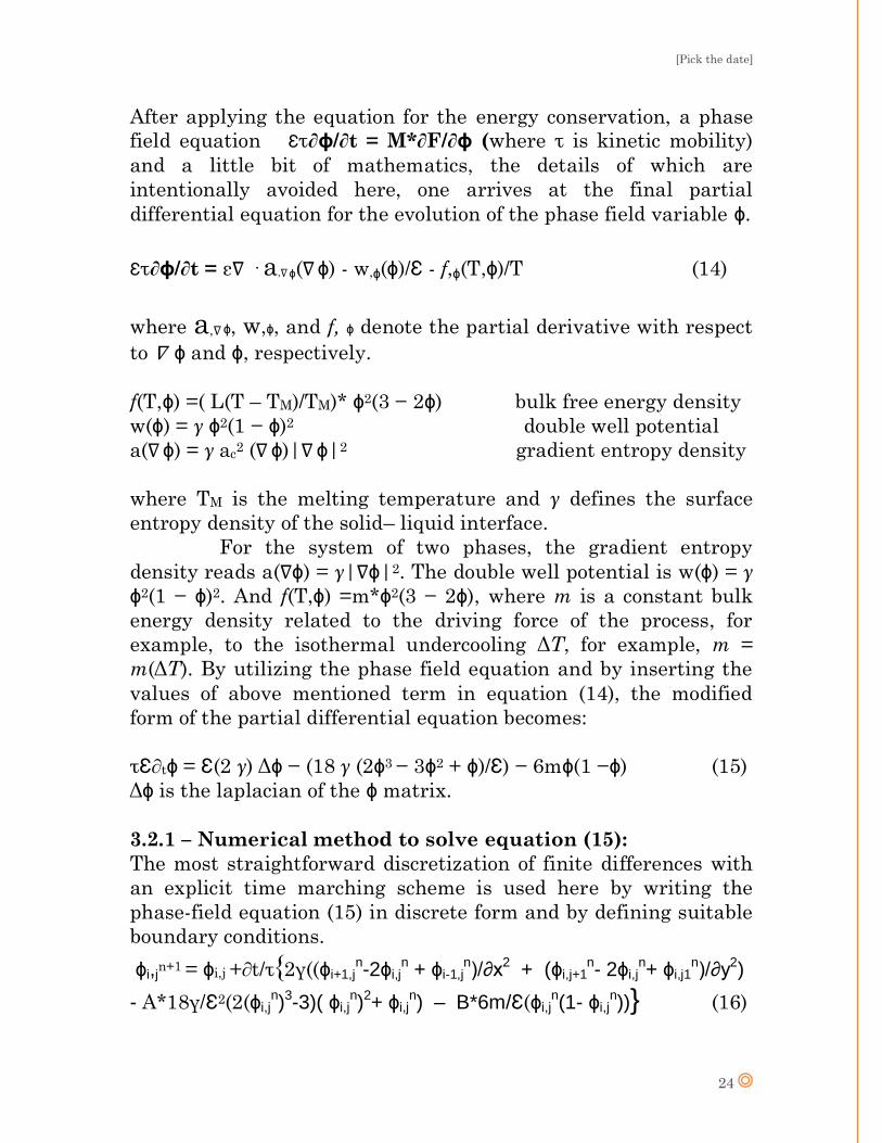
(1)Diffuse Interface Thickness: A planar solid–liquid front is
placed in the center of the domain at Nx/2 with a sharp interface
profile, with zero driving force m = 0 and with Neumann boundary
conditions on each side. The effect of different values of the small
length scale parameter: Ɛ = 1 and Ɛ = 10 responsible for the
thickness of the diffuse interface is shown in Fig. 7a, Fig 7.b
Fig 7.a
Fig 7.b
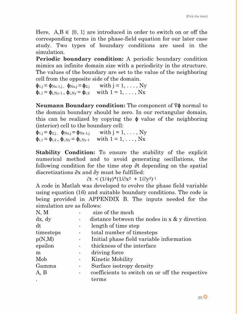
(2)Driving Force: As a next configuration, the three simulations
shown in Fig. 8a–c were performed with Ɛ = 1 with different
values of the driving force and with the initial configuration of
Fig. (a). For m = 0, the initial planar front remains stable, for

[Pick the date]
27
m = −1 the solid phase (yellow color) grows, whereas for m = 1 the
solid phase shrinks.
Fig. 8a
Fig. 8b
Fig. 8c
Fig. 8d
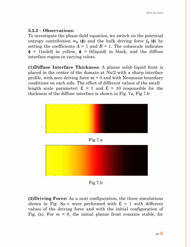
(3)Phase-Field Simulation of growing nucleus: For the
simulation in Fig. 9a, a solid nucleus is set in a 2D domain of
Nx×Ny = 100×100 grid points, with A = 1, B = 1, with driving force
[Pick the date]
28
m = −2.5 and with Neumann boundary condition. Due to periodic
boundary conditions in Fig. 9b the particle grows across the lower
boundary and appears at the top boundary.
Fig. 9a
Fig. 9b
3.3 – DEDRITIC SOLIDIFICATION:
Dendrites are formed when surface anisotropy is included in the
system, which means that now there are going to be some
preferred directions for solidification. Though there are many
models to simulate dendritic growth in the literature but in the
present report, a phase field model suggested by Ryo Kobayashi is
being studied.
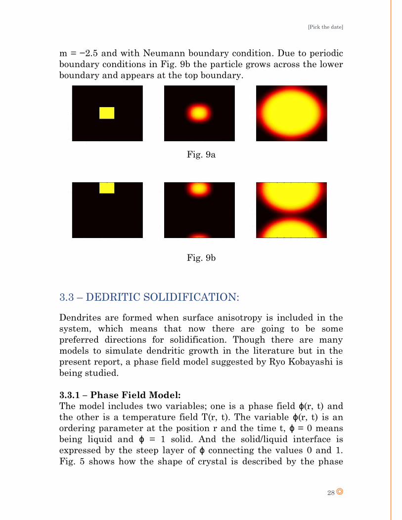
3.3.1 – Phase Field Model:
The model includes two variables; one is a phase field ϕ(r, t) and
the other is a temperature field T(r, t). The variable ϕ(r, t) is an
ordering parameter at the position r and the time t, ϕ = 0 means
being liquid and ϕ = 1 solid. And the solid/liquid interface is
expressed by the steep layer of ϕ connecting the values 0 and 1.
Fig. 5 shows how the shape of crystal is described by the phase
[Pick the date]
29
field ϕ. In order to keep the profile of ϕ such form and to move it
reasonably, we consider the following Ginzburg-Landau type free
energy functional F similar to equation (2) including m as a
parameter:
F = ʃv [f (ϕ, m) + (Ɛ2ϕ/2)*| ∇ϕ|2] dv (17)
where Ɛ is a small parameter which determines the thickness of
the layer. It is a microscopic interaction length and it also controls
the mobility of the interface. f is a double-well potential which has
local minimums at ϕ = 0 and 1 for each m. Here we take the
specific form of f as follows:
f(ϕ, m) = 1/4ϕ4 - (1/2 – 1/3*m)ϕ3 + (1/4 -1/2*m)ϕ2 (18)
Anisotropy can be introduced by assuming that Ɛ depends on the
direction of the outer normal vector at the interface. So Ɛ is
represented as a function of the vector v = vi satisfying
Ɛ(λ,v) = Ɛ(v) for λ>0. The outer normal vector is represented by -∇ϕ at the interface. Thus, we consider:
F = ʃv [f (ϕ, m) + (Ɛ(-∇ϕ )2/2)*| ∇ϕ|2] dv (19)
From the formula τ ∂ϕ/∂t = ∂f/ϕ and further simplifying, we have
the following evolution equation:
τ ∂ϕ/∂t = -∂/∂x(ƐƐ’∂ϕ/∂y)+ ∂/∂y(ƐƐ’∂ϕ/∂x) + ∇.(Ɛ2∇ϕ) + ϕ(1-ϕ)(ϕ-0.5+m)
(20)
where τ is a small positive constant and ∂Ɛ/∂v=(∂Ɛ/∂vi)i. The
parameter m gives a thermodynamical driving force. Especially in
two dimensional space, we can take Ɛ = Ɛ(θ) where θ is an angle
between v and a certain direction (for example the positive
direction of the x-axis). Ɛ’ means derivative with respect to θ.
Equation (20) gives the evolution of the order parameter or phase
field variable ϕ with time.
[Pick the date]
30
Here we assume that m is a function of the temperature T, for
example, m(T) = γ(Te - T) where Te is an equilibrium temperature,
which means that the driving force of interfacial motion is
proportional to the supercooling there. But in the following
simulations, we used the form m(T)=(α -l[γ(Te - T)] where α
and γ are positive constants; α < 1, since this assures |m(T)| < ½
for all values of T. Also m(T) is almost linear for T near Te. To
take anisotropy into account, let us specify Ɛ to be:
Ɛ = 1 + δcos(j(θ-θo)) (21)
The parameter δ means the strength of anisotropy and j is a mode
number of anisotropy. Side branching can be stimulated in the
dendrites by adding a small random noise in the equation (20).
The noise can be of the form aϕ(1-ϕ)x, where a is the strength of
noise and x is a random number in the range[-0.5,0.5].
The equation for T is derived from the conservation
law of enthalpy as:
∂T/∂t = ∇2T + K∂p/∂t (22)
T is non-dimensionalized so that the characteristic cooling
temperature is 0 and the equilibrium temperature is 1. K is a
dimensionless latent heat which is proportional to the latent heat
and inversely proportional to the strength of the cooling. For
simplicity, the diffusion constant is set to be identical in both of
solid and liquid regions. (22) is a heat conduction equation having
a heat source along the moving interface, since K∂p/∂t has
non-zero value only when the interface passes through the point.
3.3.2 – Numerical method to simulate the Dendritic growth:
The simplest finite difference scheme with a nine point laplacian
is used to solve equations (20) and (22). First, the new value of
phase field variable is calculated to substitute it into the
temperature field to get the new value of temperature field. Nine
point laplacian is required for the stability of the solution.
A code in Matlab was developed to evolve the phase
field variable and temperature field using equations (20) and (22)
[Pick the date]
31
respectively and periodic boundary conditions. The code is
attached along with this report in the CD-Drive. The inputs
needed for the simulation are as follows:
N, M - size of the mesh
dx, dy - distance between the nodes in x & y direction
dt - length of time step
timesteps - total number of timesteps
p(N,M) - initial phase field variable information
T(N,M) - initial temperature field information
K - latent Heat
TAU - phase field relaxation time
EPS - interfacial width
DELTA - strength of anisotropy
ANISO - mode number of anisotropy
ALPHA - positive constant
GAMMA - positive constant
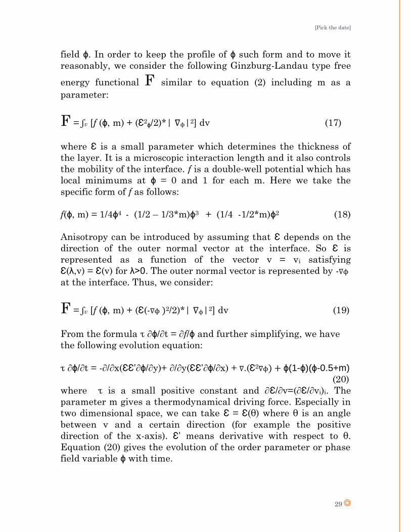
3.3.2 – Observations:
The code written in Matlab was run using the following inputs:
N= 500; M=500; dx=0.03; dy=0.03;dt=0.0003; K=4; TAU=0.0003,
EPS= 0.01; GAMMA=10.0; DELTA=0.02; ANISO=4.0;ALPHA=0.9;
Noise was not added to the system. The following was the
structure of dendrites obtained.
The yellow region indicates solid, black region indicates liquid
while the rest in indicated by the interface. Notice that there is
directional solidification in four directions because ANISO = 4.0 .
[Pick the date]
32
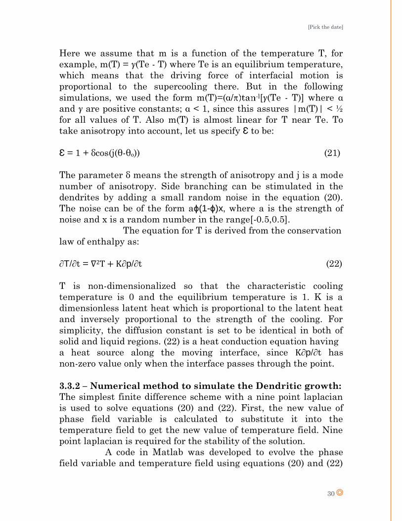
Effect of latent heat of solidification K:
The below shown four images correspond to a dimensionless latent
heat K =0.8, 1.0, 1.2 and 1.8 from left to right and top to bottom.
Notice that as the value of latent heat is increased, the dendritic
structure becomes much defined because release of latent heat is
the driving force for the process. Also noise is added to stimulate
side branching.
[Pick the date]
33
(4) CONCLUSION Phase-field models have been successfully applied to various
materials processes including solidification, solid-state phase
transformations, coarsening, and growth. With the phase-field
approach, one can deal with the evolution of arbitrary
morphologies and complex microstructures without explicitly
tracking the positions of interfaces. This approach can describe
different processes such as phase transformations and particle
coarsening within the same formulation, and it is rather
straightfoward to incorporate the effect of coherency and applied
stresses, as well as electrical and magnetic fields. Efforts are
being made in Material Science to focus on the exploration of
novel applications of the phase-field method to various materials
problems, e.g., problems involving simultaneous long-range elastic
and electric or magnetic dipole-dipole interactions, low-
dimensional systems such as thin films and multilayer structures,
and interactions between phase and defect microstructures such
as random defects and dislocations. There will also be increasing
efforts in establishing schemes to obtain the phase-field
parameters directly from more fundamental first-principles
electronic structure or atomic calculations. For practical
applications, significant additional efforts are required to develop
approaches for connecting phase-field models with existing or
future thermodynamic, kinetic, and crystallographic databases.

[Pick the date]
34
APPENDIX A MATLAB code for spinodal decomposition:
%Numerical solution of Cahn-
%Hilliard Equation via Semi-
%implicit Fourier Spectral %method for conserved
%quantities. %Non-dimensionalisation is done
%and isothermal conditions are
%considered
%For further details, refer to
%the research paper"Applications
%of semi-implicit Fourier-
%spectral method to phase field
%equations"-L.Q. Chen, Jie Shen
clear clc format long
%spatial dimensions -- adjust N
%and M to increase or decrease %the size of the computed
%solution.
N =256; M = 256; del_x = 1.0; del_y = 1.0;
%time parameters -- adjust ntmax
%to take more time steps, and %del_t to take longer time
%steps. del_t = 2.5; ntmax = 500;
%thermodynamic parameters A = 1.0; Mob = 1.0; kappa = 1.0;
%initial composition and noise
%strenght information c_0 = 0.50; noise_str = 0.5*(10^-2);
%composition used in
%calculations with a noise for i = 1:N for j = 1:M
comp(j+M*(i-1)) = c_0 +
noise_str*(0.5-rand); end end
%The half_N and half_M are
%needed for imposing the
%periodic boundary conditions half_N = N/2; half_M = M/2;
del_kx = (2.0*pi)/(N*del_x); del_ky = (2.0*pi)/(M*del_y);
for index = 1:ntmax %calculate g, g is parameterised
%as 2Ac(1-c)(1-2c) for i = 1:N for j = 1:M g(j+M*(i-1)) =
2*A*comp(j+M*(i-1))*(1-
comp(j+M*(i-1)))*(1-
2*comp(j+M*(i-1))); end end
%calculate the fourier transform
%of composition and g field f_comp = fft(comp); f_g = fft(g);
%Next step is to evolve the
&composition profile for i1 = 1:N if i1 < half_N kx = i1*del_kx; else kx = (i1-N-2)*del_kx; end kx2 = kx*kx; for i2 = 1:M if i2 < half_M ky = i2*del_ky; else ky = (i2-M-
2)*del_ky; end ky2 = ky*ky;
k2 = kx2 + ky2;
[Pick the date]
1
k4 = k2*k2; denom = 1.0 +
2.0*kappa*Mob*k4*del_t; f_comp(i2+M*(i1-1)) =
(f_comp(i2+M*(i1-1))-
k2*del_t*Mob*f_g(i2+M*(i1-
1)))/denom;
end end
%Let us get the composition back
%to real space comp = real(ifft(f_comp));
disp(comp);
disp(index);
%for graphical display of the
%microstructure evolution, %lets store the composition
%field into a 256x256 2-d
%Matrix. for i = 1:N for j = 1:M U(i,j) = comp(j+M*(i-
1)); end end %visualization of the output
figure(1) image(U*55) colormap(Jet) end disp('done');
APPENDIX B MATLAB code for isothermal solidification with no anisotropy:
% Isothermal solidifation of a
%single component liquid phase
%using explicit finite %difference scheme without any
%surface aniostropy.
% For more details, refer to
%chapter 7-Phase Field
%Modelling,Britta Nestler % -Computational Materials
%Engineering, Bernaad Jansenns.
clear clc %input parameters epsilon = 1.0; %thickness
%of the interface gamma = 1.0; %surface
%anistropy density m = -2.5; %driving
%force Mob = 1.0; %kinetic
%mobility Nx = 100; Ny = 100; %mesh size dx = 0.1; dy = 0.1; %distance
%between two consecutive nodes dt = 0.001; %length of
%time step timesteps = 100; %total
%number of time steps A = 1.0; %A and B
%are the coefiecients to switch
B = 1.0; %on and
%off the corresponding terms.
%Lets generate the initial
%picture p=zeros(Nx,Ny); for i1=Nx/2-10:Nx/2+10 for i2=Ny/2-10:Ny/2+10 p(i1,i2)=1; end end
%evolution of the order
%parameter for index=1:timesteps Lap = (4*del2(p))/(dx^2);
%Laplacian of the matrix p
for i1=1:Nx for i2=1:Ny p(i1,i2) = p(i1,i2) +
(dt/Mob)*((2*gamma*Lap(i1,i2))-
A*(18*gamma*((2*(p(i1,i2)^3))-
(3*(p(i1,i2)^2))+p(i1,i2))/(epsi
lon^2))-B*(6*m*(p(i1,i2)*(1-
p(i1,i2)))/epsilon)); end end %periodic boundary condition for i1=1:Nx p(i1,1) = p(i1,Ny-1); p(i1,Ny)= p(i1,2);
[Pick the date]
1
end for i2=1:Ny p(1,i2) = p(Nx-1,i2); p(Nx,i2)= p(2,i2); end
%neumann boundary condition %for i1=1:Nx % p(i1,1) = p(i1,2); % p(i1,Ny)= p(i1,Ny-1); %end %for i2=1:Ny % p(1,i2) = p(2,i2); % p(Nx,i2)= p(Nx-1,i2); %end %visualization of the output
disp(p) figure(1) image(p*50) colormap('hot')
end
APPENDIX C MATLAB code for dendritic solidification based on Kobayashi‟s
Model: %Phase Field Modelling of
%dendritic growth as suggested
%by Ryo Kobayashi %For more details refer to
%"Modeling and numerical
%simulationsof dendritic crystal
%growth-Ryo Kobayashi
clear clc
K = 4.0; %Latent
%heat TAU =0.0003; %PF
%relaxation time EPS =0.01; %interfacial
%width DELTA= 0.02; %modulation
%of the interfacial width ANGLEO =0.0; %orientation
%of the anisotropy axis ANISO= 4.0; %anisotropy
%2*PI/ANISO ALPHA =0.9; %m(T) =
%ALPHA/PI * atan(GAMMA*(TEQ-T)) GAMMA= 10.0; TEQ =1.0; %melting
%temperature NX= 500; %size of the
%mesh NX*NY NY =500;
H= 0.03; %spatial
%resolution DT =0.0003; %temporal
%resolution timesteps =2000000; %number of
%time steps pi =3.14159265358;
%intial temperature and phase
%field information T = zeros(NY,NX); p = zeros(NY,NX); for i1=1:NY for i2=1:NX if ((i1-NY/2)*(i1-
NY/2)+(i2-NX/2)*(i2-NX/2)<100) p(i1,i2) = 1.0; else p(i1,i2) = 0.0; end end end
%preallocation of matrices for
%faster calculations grad_p_X = zeros(NY,NX); grad_p_Y = zeros(NY,NX); aX = zeros(NY,NX); aY = zeros(NY,NX); eps2 = zeros(NY,NX);
[Pick the date]
1
angle = zeros(NY,NX); epsilon_prime = zeros(NY,NX); epsilon = zeros(NY,NX); dXdY = zeros(NY,NX); dYdX = zeros(NY,NX); grad_eps2_X = zeros(NY,NX); grad_eps2_Y = zeros(NY,NX); lap_p = zeros(NY,NX); lap_T = zeros(NY,NX);
for index=1:timesteps %calculation of all the relevant
%matrices for i1=1:NY for i2=1:NX ip = mod(i2,NX)+1; im = mod((NX+i2-
2),NX)+1; jp = mod(i1,NY)+1; jm = mod((NY+i1-
2),NY)+1; grad_p_X(i1,i2) =
((p(i1,ip) - p(i1,im))/H); grad_p_Y(i1,i2) =
((p(jp,i2) - p(jm,i2))/H); lap_p(i1,i2) =
(2.0*(p(i1,ip)+p(i1,im)+p(jp,i2)
+p(jm,i2))+p(jp,ip)+p(jm,im)+p(j
p,im)+p(jm,ip)-
12.0*p(i1,i2))/(3.0*H*H); lap_T(i1,i2) =
(2.0*(T(i1,ip)+T(i1,im)+T(jp,i2)
+T(jm,i2))+T(jp,ip)+T(jm,im)+T(j
p,im)+T(jm,ip)-
12.0*T(i1,i2))/(3.0*H*H); end end
for i1 = 1:NY for i2=1:NX if (grad_p_X(i1,i2)==0.0
&& grad_p_Y(i1,i2)>0.0) angle(i1,i2) =
0.5*pi; end if (grad_p_X(i1,i2)==0.0
&& grad_p_Y(i1,i2)<=0.0) angle(i1,i2) = -
0.5*pi; end
if (grad_p_X(i1,i2)>0.0
&& grad_p_Y(i1,i2)>0.0)
angle(i1,i2) =
atan(grad_p_Y(i1,i2)/grad_p_X(i1
,i2)); end
if (grad_p_X(i1,i2)>0.0
&& grad_p_Y(i1,i2)<=0.0) angle(i1,i2) = 2.0*pi
+
atan(grad_p_Y(i1,i2)/grad_p_X(i1
,i2)); end
if(grad_p_X(i1,i2)<0.0) angle(i1,i2) = pi +
atan(grad_p_Y(i1,i2)/grad_p_X(i1
,i2)); end end end
for i1 =1:NY for i2=1:NX epsilon(i1,i2) =
EPS*(1.0 +
DELTA*cos(ANISO*(angle(i1,i2)-
ANGLEO))); epsilon_prime(i1,i2) = -
EPS*ANISO*DELTA*sin(ANISO*(angle
(i1,i2)-ANGLEO)); end end
for i1 = 1:NY for i2=1:NX aY(i1,i2) = -
epsilon(i1,i2)*epsilon_prime(i1,
i2) * grad_p_Y(i1,i2); aX(i1,i2) =
epsilon(i1,i2)*epsilon_prime(i1,
i2) * grad_p_X(i1,i2); eps2(i1,i2) =
epsilon(i1,i2)*epsilon(i1,i2); end end
for i1=1:NY for i2=1:NX ip = mod(i2,NX)+1; im = mod((NX+i2-
2),NX)+1; jp = mod(i1,NY)+1; jm = mod((NY+i1-
2),NY)+1; dXdY(i1,i2) = (aY(i1,ip)
- aY(i1,im))/H;
[Pick the date]
2
dYdX(i1,i2) = (aX(jp,i2)
- aX(jm,i2))/H; grad_eps2_X(i1,i2) =
(eps2(i1,ip) - eps2(i1,im))/H; grad_eps2_Y(i1,i2) =
(eps2(jp,i2) - eps2(jm,i2))/H; end end
for i1=1:NY for i2=1:NX po = p(i1,i2); m = (ALPHA/pi) *
atan(GAMMA*(TEQ-T(i1,i2))); scal=
grad_eps2_X(i1,i2)*grad_p_X(i1,i
2)+
grad_eps2_Y(i1,i2)*grad_p_Y(i1,i
2); %evolution of the phase field
variable
p(i1,i2) =
p(i1,i2)+((dXdY(i1,i2)+dYdX(i1,i
2) + eps2(i1,i2)*lap_p(i1,i2)+
scal + po*(1.0-po)*(po-
0.5+m))*DT/TAU); %evolution of temperature field T(i1,i2) =
T(i1,i2)+(lap_T(i1,i2)*DT) +
(K*(p(i1,i2) - po)); end end
%visualization of the output disp(p) figure(1) image(p*50) colormap('hot')
end
Related Documents