Phase and Frequency Estimation: High-Accuracy and Low-Complexity Techniques by Yizheng Liao A Thesis Submitted to the Faculty of the WORCESTER POLYTECHNIC INSTITUTE in partial fulfillment of the requirements for the Degree of Master of Science in Electrical and Computer Engineering by May 2011 APPROVED: Professor D. Richard Brown III, Major Advisor Professor John A. McNeill, Committee Member Professor Andrew G. Klein, Committee Member

Welcome message from author
This document is posted to help you gain knowledge. Please leave a comment to let me know what you think about it! Share it to your friends and learn new things together.
Transcript

Phase and Frequency Estimation:
High-Accuracy and Low-Complexity Techniques
by
Yizheng Liao
A ThesisSubmitted to the Faculty
of theWORCESTER POLYTECHNIC INSTITUTEin partial fulfillment of the requirements for the
Degree of Master of Sciencein
Electrical and Computer Engineeringby
May 2011
APPROVED:
Professor D. Richard Brown III, Major Advisor
Professor John A. McNeill, Committee Member
Professor Andrew G. Klein, Committee Member

Abstract
The estimation of the frequency and phase of a complex exponential in additive white
Gaussian noise (AWGN) is a fundamental and well-studied problem in signal processing
and communications. A variety of approaches to this problem, distinguished primarily
by estimation accuracy, computational complexity, and processing latency, have been de-
veloped. One class of approaches is based on the Fast Fourier Transform (FFT) due to
its connections with the maximum likelihood estimator (MLE) of frequency. This thesis
compares several FFT-based approaches to the MLE in terms of their estimation accuracy
and computational complexity. While FFT-based frequency estimation tends to be very
accurate, the computational complexity of the FFT and the latency associated with per-
forming these computations after the entire signal has been received can be prohibitive in
some scenarios. Another class of approaches that addresses some of these shortcomings is
based on linear regression of samples of the instantaneous phase of the observation. Linear-
regression-based techniques have been shown to be very accurate at moderate to high signal
to noise ratios and have the additional benefit of low computational complexity and low
latency due to the fact that the processing can be performed as the samples arrive. These
techniques, however, typically require the computation of four-quadrant arctangents, which
must be approximated to retain low computational complexity. This thesis proposes a new
frequency and phase estimator based on simple estimates of the zero-crossing times of the
observation. An advantage of this approach is that it does not require arctangent calcu-
lations. Simulation results show that the zero-crossing frequency and phase estimator can
provide high estimation accuracy, low computational complexity, and low processing la-
tency, making it suitable for real-time applications. Accordingly, this thesis also presents a
real-time implementation of the zero-crossing frequency and phase estimator in the context
of a time-slotted round-trip carrier synchronization system for distributed beamforming.
The experimental results show this approach can outperform a Phase Locked Loop (PLL)
implementation of the same distributed beamforming system.

iii
Acknowledgements
First of all, I would like to express my deep and sincere gratitude to my advisor, Pro-
fessor D. Richard Brown, for providing me this great research opportunity, for giving me
the professional and insightful comments and suggestions on my research work, and for
encouraging and motivating me to move forward on the research. As an advisor, he taught
me how to start a research project, and how to face the challenges during the research work.
The research I carried out under Professor Brown has deeply motivated me to pursue my
Ph.D degree in the Electrical and Computer Engineering, and to become a faculty member
in the future.
Besides my advisor, I would also like to express gratitude to my committee members:
Professor John A. McNeill and Professor Andrew G. Klein. Thank you for reviewing my
thesis, participating in my defence, and for asking me challenging questions and giving me
professional comments on my thesis.
Most importantly, I want to say thanks to my parents. Without your encouragement
and support I would not have been able to come to the United States to study and be where
I am today. I am forever in debt to your for you unconditional love!
I would also like to thank my fellow spinlab members, Min Ni and Joshua Bacon. Thank
you for taking the time to discuss my research and help me with the experiments.
I also want to say thanks to all of my friends at WPI. Because of you, the last three
years at WPI have provided me with some of my most memorable moments in life.
Last, but not least, I am grateful for the generous support of Texas Instruments for
donating the equipment, and for the financial support of National Science Foundation.

iv
Contents
List of Figures vi
List of Tables viii
1 Introduction 1
2 Background 4
2.1 Cramer-Rao Lower Bound . . . . . . . . . . . . . . . . . . . . . . . . . . . . 52.2 FFT-Based Maximum Likelihood Estimation . . . . . . . . . . . . . . . . . 62.3 Linear-Regression-Based Maximum Likelihood Estimation . . . . . . . . . . 7
3 FFT-Based Phase and Frequency Estimation 11
3.1 Approximate Maximum Likelihood Estimation using Fast Fourier Transformand No Post-Processing . . . . . . . . . . . . . . . . . . . . . . . . . . . . . 13
3.2 Approximate Maximum Likelihood Estimation using FFT and QuadraticInterpolation . . . . . . . . . . . . . . . . . . . . . . . . . . . . . . . . . . . 18
3.3 Approximate Maximum Likelihood Estimation using FFT and Secant Method 223.4 Approximate Maximum Likelihood Estimation using FFT and Newton’s Method 31
3.4.1 Comparison of the FFT-Secant MLE and the FFT-Newton MLE . . 343.5 Approximate Maximum Likelihood Estimation using FFT and Bisection Method 373.6 Conclusion . . . . . . . . . . . . . . . . . . . . . . . . . . . . . . . . . . . . 43
4 Zero Crossing Phase and Frequency Estimation 45
4.1 Algorithm . . . . . . . . . . . . . . . . . . . . . . . . . . . . . . . . . . . . . 464.1.1 Zero-Crossing Phase and Frequency Estimator . . . . . . . . . . . . 464.1.2 Sequential Implementation . . . . . . . . . . . . . . . . . . . . . . . 48
4.2 Computational Complexity . . . . . . . . . . . . . . . . . . . . . . . . . . . 494.3 Numerical Results and Discussion . . . . . . . . . . . . . . . . . . . . . . . . 504.4 Conclusion . . . . . . . . . . . . . . . . . . . . . . . . . . . . . . . . . . . . 54
5 Zero Crossing Estimator Refinements 55
5.1 Zero Crossing Estimator using Local Linear Regression for Zero-crossings . 555.1.1 Numerical Results and Discussion . . . . . . . . . . . . . . . . . . . 59
5.2 Zero Crossing Estimator using Pre-Filtered Observation . . . . . . . . . . . 59

v
5.2.1 Numerical Results and Discussion . . . . . . . . . . . . . . . . . . . 595.3 Zero Crossing Estimator using Non-Linear Iterative Method . . . . . . . . . 62
5.3.1 Numerical Results and Discussion . . . . . . . . . . . . . . . . . . . 635.4 Conclusion . . . . . . . . . . . . . . . . . . . . . . . . . . . . . . . . . . . . 66
6 A Software-Defined-Radio Implementation of Time-Slotted Round-Trip
Carrier Synchronization for Distributed Beamforming via Zero-Crossing
Estimation 68
6.1 Two-Source Synchronization . . . . . . . . . . . . . . . . . . . . . . . . . . . 706.2 Experimental Methodology for Two-Source Test in Wire-Connected Channel 716.3 Zero-Crossing Estimator Implemented on Source Node . . . . . . . . . . . . 74
6.3.1 Implementation of the Round-Trip Time Table . . . . . . . . . . . . 746.3.2 Implementation of Zero-Crossing Estimator . . . . . . . . . . . . . . 766.3.3 Implementation of Holdover . . . . . . . . . . . . . . . . . . . . . . . 796.3.4 Implementation of FIR Filter . . . . . . . . . . . . . . . . . . . . . . 80
6.4 Data Analysis Methodology . . . . . . . . . . . . . . . . . . . . . . . . . . . 816.5 Experimental Results . . . . . . . . . . . . . . . . . . . . . . . . . . . . . . . 82
7 Conclusion 83
A The Specification of Computer and Matlab for Simulation 85
A.1 The Specification of Computer for Simulation . . . . . . . . . . . . . . . . . 85A.2 The Specification of Matlab Software for Simulation . . . . . . . . . . . . . 85
B Source Code of the TMS320C6713 Source Node in the Two-Source Sys-
tem 86
C Approximate Maximum Likelihood Estimation using Secant Method Mat-
lab Source Code 110
C.1 Main Function . . . . . . . . . . . . . . . . . . . . . . . . . . . . . . . . . . 110C.2 Function of Implementing the FFT-Secant MLE . . . . . . . . . . . . . . . 112C.3 Function of Computing A(ω) . . . . . . . . . . . . . . . . . . . . . . . . . . 114C.4 Function of Computing F
′
(ω) . . . . . . . . . . . . . . . . . . . . . . . . . . 114C.5 Function of Phase Unwrapping . . . . . . . . . . . . . . . . . . . . . . . . . 116
Bibliography 117

vi
List of Figures
3.1 Application of Maximum Likelihood Estimation. . . . . . . . . . . . . . . . 123.2 FFT MLE example with M = 212. . . . . . . . . . . . . . . . . . . . . . . . 153.3 Mean squared frequency estimation error for complex observation of FFT
MLE. . . . . . . . . . . . . . . . . . . . . . . . . . . . . . . . . . . . . . . . 163.4 Mean squared phase estimation error for complex observation of FFT MLE. 163.5 Total execution time for 500 complex observations of FFT MLE. . . . . . . 173.6 FFT-Quad MLE Example. . . . . . . . . . . . . . . . . . . . . . . . . . . . . 193.7 Mean squared frequency estimation error for complex observation of FFT-
Quad MLE. . . . . . . . . . . . . . . . . . . . . . . . . . . . . . . . . . . . . 203.8 Mean squared phase estimation error for complex observation of FFT-Quad
MLE. . . . . . . . . . . . . . . . . . . . . . . . . . . . . . . . . . . . . . . . 213.9 The Secant Method example with two iterations. . . . . . . . . . . . . . . . 233.10 FFT-Secant MLE example. . . . . . . . . . . . . . . . . . . . . . . . . . . . 263.11 Mean squared frequency estimation error for complex signal of FFT-Secant
MLE with ε = 10−4. . . . . . . . . . . . . . . . . . . . . . . . . . . . . . . . 273.12 Mean squared phase estimation error for complex signal of FFT-Secant MLE
with ε = 10−4. . . . . . . . . . . . . . . . . . . . . . . . . . . . . . . . . . . 283.13 Mean squared frequency estimation error for complex signal of FFT-Secant
MLE with ε = 10−6. . . . . . . . . . . . . . . . . . . . . . . . . . . . . . . . 293.14 Mean squared phase estimation error for complex signal of FFT-Secant MLE
with ε = 10−6. . . . . . . . . . . . . . . . . . . . . . . . . . . . . . . . . . . 303.15 FFT-Newton MLE example. . . . . . . . . . . . . . . . . . . . . . . . . . . . 333.16 Mean squared frequency estimation error for complex signal of FFT-Newton
MLE with ε = 10−4. . . . . . . . . . . . . . . . . . . . . . . . . . . . . . . . 343.17 Mean squared phase estimation error for complex signal of FFT-Newton MLE
with ε = 10−4. . . . . . . . . . . . . . . . . . . . . . . . . . . . . . . . . . . 353.18 Mean squared frequency estimation error for complex signal of FFT-bisection
MLE with ε = 10−4. . . . . . . . . . . . . . . . . . . . . . . . . . . . . . . . 393.19 Mean squared phase estimation error for complex signal of FFT-bisection
MLE with ε = 10−4. . . . . . . . . . . . . . . . . . . . . . . . . . . . . . . . 403.20 Mean squared frequency estimation error for complex signal of FFT-bisection
MLE with ε = 10−6. . . . . . . . . . . . . . . . . . . . . . . . . . . . . . . . 41

vii
3.21 Mean squared frequency estimation error for complex signal of FFT-bisectionMLE with ε = 10−8. . . . . . . . . . . . . . . . . . . . . . . . . . . . . . . . 42
4.1 State machine implementation of the zero crossing detector. . . . . . . . . . 474.2 Noisy observation with α = 0.5. . . . . . . . . . . . . . . . . . . . . . . . . . 474.3 Mean squared frequency estimation error of ZC estimator with α = 0.4. . . 514.4 Mean squared phase estimation error of ZC estimator with α = 0.4. . . . . 524.5 Mean squared frequency estimation error of ZC estimator with α = 0.2. . . 534.6 Mean squared phase estimation error of ZC estimator with α = 0.2. . . . . 53
5.1 Mean squared frequency estimation error of ZC estimator via local linearinterpolation with α = 0.4. . . . . . . . . . . . . . . . . . . . . . . . . . . . 57
5.2 Mean squared phase estimation error of ZC estimator via local linear inter-polation with α = 0.4. . . . . . . . . . . . . . . . . . . . . . . . . . . . . . . 58
5.3 Mean squared frequency estimation error of ZC estimator with α = 0.4 anda 64th order FIR filter. . . . . . . . . . . . . . . . . . . . . . . . . . . . . . . 60
5.4 Mean squared phase estimation error of ZC estimator with α = 0.4 and a64th order FIR filter. . . . . . . . . . . . . . . . . . . . . . . . . . . . . . . . 61
5.5 Mean squared frequency estimation error of ZC estimator via the SecantMethod with α = 0.4. . . . . . . . . . . . . . . . . . . . . . . . . . . . . . . 64
5.6 Mean squared phase estimation error of ZC estimator via the Secant Methodwith α = 0.4. . . . . . . . . . . . . . . . . . . . . . . . . . . . . . . . . . . . 65
6.1 Time-slotted round-trip carrier synchronization system with two source nodes. 696.2 Implementation block diagram of the two-source time-slotted round-trip car-
rier synchronization system where the blue and green lines each represents adifferent signal wired path . . . . . . . . . . . . . . . . . . . . . . . . . . . . 72
6.3 Effect of multipath on ZC estimation and holdover. . . . . . . . . . . . . . . 81

viii
List of Tables
4.1 Phase of a complex exponential at zero crossing . . . . . . . . . . . . . . . . 464.2 Computational Complexity of Tretter, Kay, and zero-crossing estimators . . 50
6.1 Two-source round-trip synchronization protocol timing. After detection ofthe primary beacon, each node keeps time using its sample clock running at16 kHz. . . . . . . . . . . . . . . . . . . . . . . . . . . . . . . . . . . . . . . 73
6.2 Experimental results of two-source wired-channel tests. Each experimentconsisted of 100 distributed beamforming tests. . . . . . . . . . . . . . . . . 82
A.1 The Specification of simulation computer . . . . . . . . . . . . . . . . . . . 85A.2 The Specification of Matlab . . . . . . . . . . . . . . . . . . . . . . . . . . . 85
1
Chapter 1
Introduction
The estimation of the frequency and phase of a complex exponential in additive white
Gaussian noise (AWGN) is a fundamental and well-studied problem in signal processing
and communications. Its numerous applications include carrier recovery in a communi-
cation system [1], determination of the object position in radar and sonar systems [2, 3],
estimation of the heart rate of a fetus in biomedicine [4], and carrier synchronization in
a distributed beamforming system [5]. Regardless of the application, poor estimation can
lead to disastrous results. For example, in communication system, with the poor carrier
frequency estimate, the down-converter may not be able to demodulate the passband signal
to baseband [1]. In the smart antenna system and speech processing system, a poor phase
estimator may cause the system to fail to identify the direction of arrival of the signal [6, 7].
Nowadays, a variety of approaches to the frequency and phase estimation problem,
distinguished primarily by estimation accuracy, computational complexity, and process-
ing latency, have been developed. One class of approaches is based on the Fast Fourier
Transform (FFT) due to its connections with the maximum likelihood estimation (MLE)
of frequency. The MLE has very high accuracy because it achieves the Cramer-Rao Lower
Bound (CRLB), which is the minimum possible error for the unbiased estimator, over a
wide range of Signal-to-Noise Ratio (SNR) values. Several FFT-based MLEs have been
proposed in [8], [9], [10], [11], and [12]. However, none of the literature compares the com-
putational complexity of each approach. Therefore, in this thesis, we compare the accuracy

2
and the computational complexity of the approach given in [8] and its refinements. The
results show that by using the root-finding algorithms the accuracy of the FFT-based MLE
is improved significantly. Also, the computational complexity is reduced by avoiding the
FFT with a large number of points. Although the FFT-based MLE can provide a high
accuracy of estimation, the latency can be prohibitive in some scenarios because the FFT
can only be performed after receiving the entire signal.
Another class of approaches that addresses the shortcomings of the FFT-based MLEs
is based on linear regression of samples of the instantaneous phase of the observation.
Several approaches have been proposed in [13], [14], [15], and [16]. Linear-regression-based
techniques have been shown to be very accurate at moderate to high SNRs. In addition,
some of the approaches have been shown to have low computational complexity and low
latency due to the fact that the processing can be performed on a sample-by-sample basis.
These techniques, however, typically require the computation of four-quadrant arctangents,
which must be approximated to retain low computational complexity. In this thesis, we
propose a new frequency and phase estimator called the zero-crossing phase and frequency
estimator. The proposed estimator is based on the simple estimates of the zero-crossing
times of the observation. Compared with the estimators presented in [13] and [14], our
approach has similar performance, but lower computational complexity. Our proposed
estimator avoids the arctangent operation by using the instantaneous phase of each zero
crossing, which is known. In addition, rather than computing the instantaneous phase
of each received sample, our approach only computes the instantaneous phase of the zero
crossings. Therefore, less operations are required. Furthermore, our approach has low
latency because it can be implemented in a sequential way. Due to its high accuracy, low
computational complexity, and low processing latency, the proposed zero-crossing estimator
is suitable for real-time applications.
To demonstrate the real-time applicability of the zero-crossing phase and frequency
estimator, this thesis also presents a real-time implementation of the zero-crossing phase
and frequency estimator in the context of a distributed beamforming system utilizing the
time-slotted round-trip carrier synchronization protocol. Compared with the experimental
results of the same distributed beamforming system implemented via a hybrid Phase Locked

3
Loop (PLL) in [17], our approach offers less signal power lost at the destination. Also, our
experimental results are more consistent.
The rest of this thesis is organized as follows. Chapter 2 introduces the Cramer-Rao
Lower Bound and gives a review of FFT-based and linear-regression-based estimations.
Chapter 3 discusses the FFT-based maximum likelihood estimation and its refinements by
using quadratic interpolation and root-finding algorithms. For each estimator in Chapter 3,
we provide numerical results as a function of SNR. In addition, the computational complex-
ity is discussed for each estimator. Chapter 4 proposes the algorithm of the Zero-Crossing
phase and frequency estimator, and also compares numerical results with Tretter’s estimator
and Kay’s estimator. Chapter 5 presents three refinements of the proposed ZC estimator.
Each refinement is analysed numerically, and the performance is compared with the fun-
damental zero-crossing estimator, Tretter’s estimator, and Kay’s estimator. In Chapter 6,
the zero crossing estimator is implemented in a time-slotted round-trip carrier synchroniza-
tion distributed beamforming system by software-defined-radio in a wire-connected chan-
nel. Finally, the software implementation of the zero crossing algorithm is discussed and
the methodology of the experiment is given. This thesis then concludes with experimental
results from this chapter.

4
Chapter 2
Background
In the problem of estimating the unknown parameters of a single tone in noise from the
discrete-time observations, we consider the complex-valued received signal
z[n] = b0 exp(j(ω0nT + θ0)) + w[n] (2.1)
for n = n0, . . . , n0 + N − 1, where frequency ω0, ω0 ≥ 0, amplitude b0, and phase offset
θ0, −π ≤ θ0 < π, are unknown constants. The variable T denotes the sampling period, n0
denotes the index of the first sample, and w[n] is a zero-mean proper complex Gaussian
random variable with var <(w[n]) = var =(w[n]) = σ2. The covariance of <(w[n]) and=(w[n]) is zero. Therefore, we assume that w[n] are independent and identically distributed
(i.i.d) for n = n0, n0 + 1, . . . , n0 + N − 1. The Signal-to-Noise ratio (SNR) is defined as
SNR :=b202σ2 .
The N -sample observation of (2.1) is provided as an input to a phase and frequency
estimator. The phase and frequency estimates generated by the estimators are denoted as
θ and ω respectively. The resulting phase and frequency errors are denoted as θ := θ0 − θ
and ω := ω0 − ω, respectively.

5
2.1 Cramer-Rao Lower Bound
In this paper, we use the Cramer-Rao Lower Bound (CRLB) as a benchmark for the
performance of an estimator. An unbiased estimator that achieves the CRLB is said to be
“efficient” , in the sense that it achieves the best possible performance in the context of
a squared-error cost. The Fisher information matrix for the CRLB for complex signal is
[8, 12]
J(β) :=1
σ2
b20T2(n2
0N + 2n20P +Q) 0 b20T (n0N + P )
0 N 0
b20T (n0N + P ) 0 b20N
(2.2)
where β = [ω0, b0, θ0]T ,
P :=
N−1∑
n=0
n =N(N − 1)
2(2.3)
Q :=N−1∑
n=0
n2 =N(N − 1)(2N − 1)
6and
β := [ω0, b0, θ0]T . (2.4)
When all three parameters are unknown, after inverting all the variations of the information
matrix J, the variances obtain the following set of bounds:
varb0 ≥ σ2
N(2.5)
varω0 ≥ 12σ2
b20T2N(N2 − 1)
(2.6)
varθ0 ≥ 12σ2(n20N + 2n0P +Q)
b20N2(N2 − 1)
(2.7)

6
The CRLB for the covariance of the frequency and phase errors of a complex exponential
in AWGN when both of the phase and frequency are unknown is given as [8]
cov
[
ω, θ]T
≥ σ2
b20
NT 2(NP−Q2)
−(Nn0+P )T (NP−Q2)
−(Nn0+P )T (NP−Q2)
Nn20+2n0P+Q(NP−Q2)
.
(2.8)
where the notation A ≥ B means that A−B is positive semi-definite. In order to isolate the
phase and frequency errors, we choose the first sample index n0 = −P/N , the off-diagonal
terms of (2.8) can be set to zero and the frequency and phase estimation performance of
each algorithm can be evaluated independently.
2.2 FFT-Based Maximum Likelihood Estimation
The maximum likelihood (ML) frequency estimator given the observation (2.1) is [8]
ωML = argmaxω∈Ω
|A(ω)| (2.9)
where Ω ⊆ [0,∞), and
A(ω) =1
N
N−1∑
n=0
z[n] exp(−jnωT ). (2.10)
After finding ωML, the phase estimate is computed by using the follow equation
θML = ∠ exp(−jωMLt0)A(ωML) (2.11)
where t0 := n0T . The amplitude is estimated by using
b0ML = |A(ωML)| (2.12)
A well-known numerical method to locate ωML is given in [8]. In order to locate ωML,
they use the discrete Fourier transform (DFT) to find ω which approximately maximizes
|A(ω)|. In fact, the M -point DFT is a sampled version of A(ω) at frequencies ω = 2πkMT for
k := 0, ...,M − 1. Usually, the Fast Fourier transform (FFT) is used to compute A( 2πkMT )

7
for k := 0, ...,M − 1. Then they select the index k at which A( 2πkMT ) attains its maximum
magnitude. In other words, (2.9) is maximized over a discrete set rather than Ω. Then the
frequency estimate can be computed as
ωRife =2πk
MT. (2.13)
After finding ωRife, we can use (2.11) and (2.12) to find the phase and amplitude estimates.
As presented in [8], when none of the frequency, phase, and amplitude is known, the
proposed estimator computes the frequency estimate as first. Then the phase and amplitude
estimates are computed based on the frequency estimate. Therefore, the accuracy of the
frequency estimator is very important. With a poor frequency estimator, it is difficult to
have a good phase and amplitude estimates. Thus, in [8], Rife and Boorstyn proposed
a two-part search routine. The first part is called the coarse search which uses the FFT
method discussed above to locate the ω. The second part locates the local maximum closet
to the value of ω picked out by the first part. This part is called the fine search. If
the frequency estimate computed by coarse search is accurate, this procedure will locate
the global maximum of |A(ω)| and thus the best approximate ML estimates. In [8], the
Secant method is used for the fine search. However, few details are provided about how to
implement it. In Section 3.3, a detailed study is provided about using the FFT and the
Secant Method to implement the approximate maximum likelihood estimation.
2.3 Linear-Regression-Based Maximum Likelihood Estima-
tion
In the previous section, the discussed maximum likelihood estimator uses the FFT to
locate the estimate ωML approximately, which maximizes the likelihood function |A(ω)|. Forthe proposed method in [8], the estimator needs to process after receiving all the samples.
It is not an efficient algorithm for the applications require low latency. In addition, the
computational complexity of the FFT isO(M logM), whereM is the number of FFT points.
This computation of the FFT will increase the latency of estimation as well. Nowadays,

8
more and more applications require a low-latency algorithm for computation. One of the
well-known solutions is the linear-regression-based maximum likelihood estimation. For this
category of estimation, the estimators find the phase of the received observation, i.e.
φ[n] := ∠z[n] = ω0nT + θ0, (2.14)
and then apply the linear regression to φ[n]|n = n0+0, n0+1, . . . n0+N−1 for estimating
ω and θ. Most of the proposed algorithms can attain the CRLB over a wide range of SNR
values.
Tretter is the first person to present the idea of using phase samples to estimate frequency
and phase [13]. The observed signal in (2.1) can be expressed as
z[n] = 1 + v[n] b0 exp(j(w0nT + θ0)) (2.15)
where
v[n] =1
b0w[n] exp(−j(w0nT + θ0)). (2.16)
Let v[n] = vR[n] + jvI [n], then
1 + v[n] =
1 + vR[n]2 + v2I [n]1/2
× exp
j arctanvI [n]
1 + vR[n]
(2.17)
For high SNR, when 1 vR[n] and 1 vI [n], we can write
(1 + v2R[n])2 + v2I [n]1/2 ' 1 (2.18)
and
1 + v[n] ' exp j arctan vI [n] ' jvI [n] . (2.19)
Hence, 1 + v[n] ' jvI [n].

9
This approximation can then be plugged back into (2.15) to write
z[n] ' b0 exp j(w0nT + θ0 + vI [n]) . (2.20)
All the required information is contained in the phase angle of (2.20)
φ[n] := ω0nT + θ0 + vI [n]. (2.21)
(2.21) can be computed by applying a phase unwrapping algorithm and using an arctangent
operation, i.e. φ[n] = unwraparctanz[n]. The parameters ωtretter and θtretter can be
calculated by least squares (LS) regression, i.e.
ωtretter
θtretter
=12
T 2N2(N2 − 1)
×
N −T (Nn0 + P )
−T (Nn0 + P ) T 2(Nn20 + 2n0P +Q)
×[
n0+N−1∑
n=n0
nTφ(n)n0+N−1∑
n=n0
φ(n)
]
. (2.22)
As discussed in [13], Tretter’s estimator can only achieve the CRLB as a sufficiently high
SNR.
Compared with the Rife’s MLE, Tretter’s estimator does not require to use the FFT.
Instead, linear regression is applied to the phase of each sample. Therefore, the computa-
tional complexity is reduced. In addition, based on (2.22), the proposed estimator can be
implemented in sequence. This advantage makes it possible to implement Tretter’s estima-
tor with low latency. However, the phase unwrapping is not an efficient operation, which
may increase the computational complexity. In addition, the phase unwrapping algorithm
may fail at low SNR [14].
In [14], Kay proposed a similar algorithm which still uses the phase of each sample for
estimation, but avoids the phase unwrapping by using the differenced phase of two adjacent

10
points. From (2.20) and (2.21), we have
∆[n+ 1] = ∠z[n+ 1]− ∠z[n]
= φ[n+ 1]− φ[n]
= ω0T + vI [n+ 1]− vI [n] (2.23)
When SNR is high, we know 1 vI [n]. Therefore, vI [n + 1] − vI [n] ' 0. Thus, as long as
SNR is high enough, we can apply the least square regression again to (2.23) to estimate ω.
In [14], an alternative approach is introduced. Since ∠z[n+1]−∠z[n] = ∠ z[n+ 1]z∗[n],in addition the noise vI [n] is coloured noise, the standard weighted least-squares theory [18]
leads to a weighted average estimate, given by
ωkay =1
(N − 1)T
N−2∑
n=0
p[n] arg z∗[n]z[n + 1] (2.24)
where
p[n] =6(n + 1) [N − (n+ 1)]
N(N2 − 1). (2.25)
As shown in [14], Kay’s estimator can only attain the CRLB at high SNR. The unweighed
Kay’s estimator is very close to the CRLB but not attain it. In addition, compared with
the FFT-based MLE, the threshold of Kay’s estimator is larger.
In [14], the estimator for θkay is not given. Since the least square estimation is equivalent
to ML method when the estimate is unbiased, hence, we use (2.11) for phase estimation,
i.e.
θkay = arg exp(−jωkayn0)A(ωkay) (2.26)
Compared with Tretter’s estimate, Kay’s estimate does not require to use the phase un-
wrapping algorithm, which makes the computation more efficient. In [13], the author does
not give a specific phase unwrapping algorithm for Tretter’s method. In [19], the author
shows that Kay’s method is equivalent to Tretter’s method with Itoh’s phase unwrapping
algorithm.

11
Chapter 3
FFT-Based Phase and Frequency
Estimation
The Maximum Likelihood Estimator (MLE) has many applications in the estimation of
unknown parameters of a complex exponential because it is asymptotically efficient [18], i.e.
it achieves the CRLB as the number of samples becomes large. Many articles, such as [8],
[10], and [18], have discussed the methods to search for the value of the unknown variable
which maximizes the likelihood function (3.2). However, all of the methods are required to
know the entire signal before estimation. Therefore, the MLE is not the primary choice for
the applications that require fast estimation or computationally-constrained applications.
In some applications, the MLE can be used to analyse and to evaluate the performance of
other estimation techniques when the “truth” is not known. In order to do that, the Mean
Squared Error (MSE) of the ML frequency estimator, which is defined as E[(ω0 − ω)2],
and the MSE of ML phase estimator, which is defined as E[(θ0 − θ)2], where E denotes
the expectation, have to be significantly better than the estimator of interest. The best
any unbiased estimator can do is attaining the CRLB over a wide range of SNR values,
especially at high SNR.
Figure 3.1 shows an application using the MLE to analyse a hybrid Phase Locked Loop
(PLL) algorithm for the carrier synchronization of the distribute beamforming [17, 20]. In
this test, two software-defined radios (SDRs) are used as transmitter and receiver separately.

12
Transmitter Receiver
ML Estimator
PLL
MSE
Signal
Generator
Tx[n] Rx[n]
Figure 3.1: Application of Maximum Likelihood Estimation.
The Signal Generator produces the sinusoidal beacon Tx[n] = cos(nTω + θ), where ω is
known frequency and θ is known phase offset. The transmitter reconstructs the beacon
Tx[n] and then sends it to the receiver. After receiving the beacon, the receiver samples
the received signal and then sends the sampled signal Rx[n] = cos(nT ω + θ) to the PLL
estimator. After convergence, the PLL estimator outputs the frequency and phase estimates,
ωPLL and θPLL respectively. Finally, we compute the frequency MSE, E[(ω− ωPLL)2], and
the phase MSE, E[(θ − θPLL)2]. In this test, we do not know the true ω and θ. Therefore,
we need to have an estimator with high accuracy to compute the best possible true values of
ω and θ. As discussed in [18], the maximum likelihood estimator is asymptotically efficient.
Therefore, this estimator can be used to compute ω and θ when the number of samples is
large. As shown in Figure 3.1, the received signal Rx[n] is also sent to the ML estimator.
The outputs of the ML estimator are ωML and θML. Due to its high accuracy, we assume
ω = ωML and θ = θML. Hence, now we have enough knowledge to evaluate the performance
of the hybrid PLL.
The example presented above is not singular. There are many other applications requir-
ing a high accurate estimator. However, as discussed in Section 2.2, the frequency estimate
ωML requires numerical methods to compute. Therefore, five approximate maximum like-
lihood estimators are proposed and discussed in this chapter. They are:
1. Approximate maximum likelihood estimator using Fast Fourier Transform (FFT) and
no post-processing (FFT estimator)
2. Approximate maximum likelihood estimator using FFT and quadratic interpolation
(FFT-Quad estimator)

13
3. Approximate maximum likelihood estimator using FFT and Secant method (FFT-
Secant estimator)
4. Approximate maximum likelihood estimator using FFT and Newton’s method (FFT-
Newton estimator)
5. Approximate maximum likelihood estimator using FFT and bisection method (FFT-
bisection estimator)
All the estimation techniques are based on the FFT. The only difference among them is the
post-processing after the FFT. For instance, the FFT-Quad estimator uses the quadratic
interpolation to compute the unknown parameters after FFT. The FFT-Secant estimator
and the FFT-Newton estimator use different root-finding algorithms to estimate the un-
known parameters. For each estimator, we will evaluate the frequency and phase MSEs as
a function of SNR. Also, we will discuss the computational complexity of each algorithm.
At the end of this chapter, we will summarize the performance and finally give a guideline
for choosing the algorithm for approximate MLE.
3.1 Approximate Maximum Likelihood Estimation using Fast
Fourier Transform and No Post-Processing
As discussed in Section 2.2, the frequency estimate of the maximum likelihood estimator
is
ωML = argmaxω∈Ω
|A(ω)| (3.1)
where
A(ω) =1
N
N−1∑
n=0
z[n] exp(−jnωT ) (3.2)
and Ω ⊆ [0,∞).
In [8] and [9], Rife presents an approximate method which uses the Discrete Fourier
Transform (DFT) to approximately locate the value of ω, which maximizes |A(ω)|. In fact,
the M -point DFT is a sampled version of A(ω) at frequencies ω = 2πkMT for k ∈ K and

14
K := 0, 1, . . . ,M − 1. Usually, we use the Fast Fourier Transform (FFT) to compute
A( 2πkMT ) for k ∈ K [8]. Hence, (3.1) becomes to
k = argmaxk∈K
∣
∣
∣
∣
A
(
2πk
MT
)∣
∣
∣
∣
. (3.3)
After finding k, we can form an approximate estimate ωML, ωFFT , by using (3.4)
ωFFT =2πk
MT, (3.4)
which requires an exhaustive search, but over a finite set of discrete points. Then the
approximate phase θFFT can be estimated by using (3.5)
θFFT = ∠exp(−jωFFT t0)A(ωFFT ) (3.5)
where t0 := n0T .
In order to show how the FFTML estimator works, we present a numerical example here.
For example, an observation without noise has N = 513 samples, sampling period T = 1
second, first sample index n0 = −256, the frequency ω0 = 0.1 × 2π = 0.6283 rad/second
(rad/s) and the phase offset θ0 = 0 rad. We use a M = 212 points FFT to estimate the
frequency. As shown in Figure 3.2, the peak is located at k = 410. After calculation by
using (3.4), we find ωFFT = 0.6289 rad/s, and θFFT = 0 rad, which is as same as θ0. The
squared frequency estimate error is 3.7650 × 10⁻⁷.
If we increase M to 214, the peak is located at k = 1638. Then ωFFT = 0.6282 rad/s,
which is much closer to ω0, and θFFT = 0 rad. The squared error of the frequency estimate
is 2.3531 × 10⁻⁸, which is improved by 10 times from the previous case. If we increase M
to 218, the peak is located at k = 26214. Then ωFFT = 0.6283 rad/s and θFFT = 0 rad.
The squared frequency estimate error is again improved to 9.1918 × 10⁻¹¹.
Figure 3.3 and Figure 3.4 show the MSE of the frequency and phase estimates of the FFT
MLE respectively as a function of SNR := 10 log10(b20/2σ
2) for five values of M , M = 210,
M = 212,M = 214,M = 216, and M = 220, for a complex observation with AWGN. All the
results assume an observation with N = 513, sampling period T = 1 second, and the first

15
400 405 410 415 4200
0.2
0.4
0.6
0.8
1
index
|A|
Figure 3.2: FFT MLE example with M = 212.
sample time n0 = −256. The frequency is an independent random variable for a uniform
distribution
ω0 ∼ U(0.09 × 2π, 0.11 × 2π). (3.6)
The phase is an independent random variable for a uniform distribution
θ0 ∼ U(−π, π). (3.7)
500 realizations of the random complex exponential signal using (2.1) and AWGN are gen-
erated with fixed b0 = 1.
In Figure 3.3, the estimators with M = 210 and M = 212 fail to track on the CRLB
over the entire SNR range. The low-SNR threshold of all of the rest estimators is a SNR of
about -9dB. The estimator with M = 214 closely tracks the CRLB up to a SNR of about
0dB. The estimator with M = 216 closely tracks the CRLB up to a SNR of about 12dB. For
the estimator with M = 220, the estimation range is much wider than other four estimators.

16
−10 0 10 20 30 40 50 6010
−15
10−10
10−5
100
SNR(dB)
mea
n sq
uare
d fr
eque
ncy
estim
atio
n er
ror
M = 210
M = 212
M = 214
M = 216
M = 220
CRLB
Figure 3.3: Mean squared frequency estimation error for complex observation of FFT MLE.
−10 0 10 20 30 40 50 6010
−10
10−8
10−6
10−4
10−2
100
SNR(dB)
mea
n sq
uare
d ph
ase
estim
atio
n er
ror
M = 210
M = 212
M = 214
M = 216
M = 220
CRLB
Figure 3.4: Mean squared phase estimation error for complex observation of FFT MLE.

17
It tracks the CRLB for up to a SNR of about 38dB. In Figure 3.4, which shows the phase
estimation performance, all of the estimators can track the CRLB from -9dB to 60dB.
2^10 2^12 2^14 2^16 2^18 2^2010
−1
100
101
102
Number of FFT points
Exe
cutio
n tim
e fo
r 50
0 ob
serv
atio
ns
Figure 3.5: Total execution time for 500 complex observations of FFT MLE.
Figure 3.3 shows that an increase of the value of M can improve the estimation accuracy.
However, when we increase M , the execution time also increases. Figure 3.5 shows the total
execution time for 500 complex observations of the FFT MLE. As shown in the figure, the
execution time increases when M increases. For the FFT MLE, the most time consumption
part is the computation of FFT. The computational complexity of the FFT is O(M logM).
If we increase M from M = 212 to M = 214, the execution time will be increased by a
factor of 4.67. Figure 3.5 shows that if we increase M from 212 to 220, the execution time is
increased by more than 100 times. One thing we should notice is since the Matlab uses the
multiple threads computation automatically, the plot in Figure 3.5 does not exactly follow
the ratio of M logM . In addition, memory space is an issue when using a large value of M .
In our simulation, we use double precision complex variable to store the output of one FFT
computation. Assume each double precision complex variable requires 128 bits. Then for

18
a 214 points FFT, we need 256 KB memory to store the values. For a 220 points FFT, we
need 32 MB memory to store the values. If we want to use single 228 points FFT, we need
to have a 4 GB memory to store the variables. Therefore, in order to achieve high accuracy,
the FFT ML estimator requires a high performance computer with large memory space.
3.2 Approximate Maximum Likelihood Estimation using FFT
and Quadratic Interpolation
Let us reconsider the FFT MLE example with M = 212 from Section 3.1. When ω0 =
0.1× 2π = 0.6283 rad/s, by using (3.8), we find that the peak of |A(ω)| is located between
k = 409 and k = 410.
kML =ω0MT
2π=
0.2π × 212 × 1
2π= 409.6 (3.8)
However, the index of FFT cannot be an non-integer number. Therefore, in order to improve
the accuracy, one approach is to interpolate between points near the peak of the FFT. In
[12], the FFT magnitude is interpolated by quadratic polynomial to improve the estimation
accuracy. For example, we find the peak of FFT locates at FFT index k. A quadratic
fit y = a + bx + cx2 in the neighbourhood of the maximum can be computed given the
frequencies x ∈
2π(k−1)MT , 2π(k)MT , 2π(k+1)
MT
and FFT magnitudes y = |A(x)|. Then the peak
of the quadratic fit, which is also the frequency estimate, is ωQuad = −b2c . Finally, we can
estimate phase θQuad by using (3.10). This method is described as the FFT-Quad MLE in
this thesis.
We use the example inFigure 3.2 to demonstrate how the FFT-Quad MLE works. We
use a M = 212 points FFT estimator to locate the peak at k = k1 = 410, as shown in Figure
3.6.
We can compute the quadratic polynomial coefficients a, b, c by solving the linear system

19
405 406 407 408 409 410 411 412 413 414 4150.9
0.92
0.94
0.96
0.98
1
index
|A|
FFT Plotk
ML
Quadratic Interpolation
Figure 3.6: FFT-Quad MLE Example.
(3.9),
(
2π(k−1)MT
)22π(k−1)
MT 1(
2π(k)MT
)22π(k)MT 1
(
2π(k+1)MT
)22π(k+1)
MT 1
c
b
a
=
|A(2π(k−1)MT )|
|A(2π(k)MT )||A(2π(k+1)
MT )|
(3.9)
which gives an exact quadratic fit to the data. The matrix on the left is commonly referred
as a Vandermonde matrix [21]. After solving the linear system in (3.9), we compute ωQuad =
−b2c , which is the peak of the quadratic fit and also the frequency estimate.
In our example, the maximum found by the quadratic interpolation is ωQuad = 0.6283.
Then, we can estimate θQuad by calculating (3.10)
θQuad = ∠exp(−jωQuadt0)A(ωQuad) = 0. (3.10)
The associated squared error of the frequency estimate is 2.9591 × 10⁻¹². This squared

20
error is much smaller than that of the FFT estimator with the same M value and also
smaller than that of the FFT estimator with M = 218.
Figure 3.7 and Figure 3.8 show the MSE of the frequency and phase estimates of the
FFT-Quad ML respectively as a function of SNR for different values of M, for a complex
observation with AWGN. All the results assume an observation with N = 513, sampling
period T = 1 second, and the first sample time n0 = −256. The frequency and phase are
independent random variables for the uniform distributions (3.6) and (3.7) respectively. 500
realizations of the random complex exponential signal using (2.1) and AWGN are generated
with fixed b0 = 1. Since we have known that with the increase of the value of M , the
accuracy of the estimation will be improved as well. Hence, we only consider about the
cases with small values of M . Here we only consider M = 210, M = 212, and M = 214.
−10 0 10 20 30 40 50 6010
−15
10−10
10−5
100
SNR(dB)
mea
n sq
uare
d fr
eque
ncy
estim
atio
n er
ror
M = 210
M = 212
M = 214
CRLB
Figure 3.7: Mean squared frequency estimation error for complex observation of FFT-QuadMLE.
In Figure 3.7, all estimators have the same threshold, which is -9dB. However, the
estimator with M = 210 fails to achieve the CRLB after 0dB. Compared with the FFT

21
−10 0 10 20 30 40 50 6010
−10
10−8
10−6
10−4
10−2
100
SNR(dB)
mea
n sq
uare
d ph
ase
estim
atio
n er
ror
M = 210
M = 212
M = 214
CRLB
Figure 3.8: Mean squared phase estimation error for complex observation of FFT-QuadMLE.

22
MLEs, the estimators with M = 212 and M = 214 have a wider estimation range. The
former one tracks the CRLB up to a SNR of about 38dB. And the latter one tracks the
CRLB up to a high SNR of 60dB. Figure 3.8 shows that all of the phase estimators can
attain the CRLB.
Compared with Figure 3.3 and Figure 3.4, Figure 3.7 and Figure 3.8 show that the es-
timation accuracy is improved by a significant level because of the quadratic interpolation
post-processing. In order to form the Vandermonde matrix in (3.9), we need four multi-
plications. The computational complexity of matrix inversion via Gaussian Elimination is
O(N3) and the approximate number of operations is 2n3/3 [22]. Therefore, for a 3 × 3
matrix, the number of operations of matrix inversion is 18. For the matrix multiplication,
the number of multiplication is 27. Therefore, finally, the computational complexity for
FFT-Quad MLE is O(M logM) + 45 ' O(M logM) +O(1).
3.3 Approximate Maximum Likelihood Estimation using FFT
and Secant Method
In [8] and [9], the maximum likelihood estimation search routine has two parts. The
first search part is called the coarse search, which is the FFT MLE described in Section 3.1.
The accuracy of the coarse search is strongly affected by the number of points of FFT, as
discussed in Section 3.1. In order to improve the estimation accuracy, the coarse search is
followed by a fine search. One example of a fine search is the FFT-Quad MLE presented in
Section 3.2. In [8], another fine search approach was described: the Secant method. This
section discusses the Secant method and its application to ML frequency estimation.
The Secant method is a iterative method used to find roots of a equation f : < → <.The iteration formula is [23]
x(m) :=x(m−2)f(x(m−1))− x(m−1)f(x(m−2))
f(x(m−1))− f(x(m−2)), m ≥ 2
= x(m−1) − f(x(m−1))x(m−1) − x(m−2)
f(x(m−1))− f(x(m−2)). (3.11)
The two initial values, x(0) and x(1), are chosen to lie close to the desired root. As shown

23
in Figure 3.9, we want to find the root of y = 4(x + 1)(x − 0.5)(−x + 2)(−x + 2.8) near
x = 0.5. We picked up the initial point x(0) = 1.5 and x(1) = −0.5. Then we apply (3.11)
to compute x(2) and continue. After two iterations, x(3) converges to a value which is very
close to the root at x = 0.5.
−1 −0.5 0 0.5 1 1.5 2 2.5−20
−15
−10
−5
0
5
10
x
f(x)
x0x1
x2x3
Figure 3.9: The Secant Method example with two iterations.
Finding ω which maximizes |A(ω)| is equivalent to finding a root of the first order
derivative of |A(ω)| or a root of the first order derivative of |A(ω)|2. The DFT in (2.10) can
be written in rectangular form as:
A(ω) := B(ω) + jC(ω) (3.12)
where
B(ω) :=1
N
N−1∑
n=0
βn cos(nωT ) + γn sin(nωT ), (3.13)
C(ω) :=−1
N
N−1∑
n=0
βn sin(nωT )− γn cos(nωT ), (3.14)

24
and where
βn = <z[n] and (3.15)
γn = =z[n]. (3.16)
Hence,
F (ω) := |A(ω)|2 = A(ω)A∗(ω) = B2(ω) + C2(ω). (3.17)
Now, we have
F ′(ω) =dF
dω:= 2B
dB
dω+ 2C
dC
dω(3.18)
wheredB
dω:=
T
N
N−1∑
n=0
n(−βn sin(Tnω) + γn cos(Tnω))
dC
dω:=
−T
N
N−1∑
n=0
n(βn cos(Tnω) + γn sin(Tnω))
Therefore, (3.11) becomes
ω(m) = ω(m−1) − F′
(ω(m−1))ω(m−1) − ω(m−2)
F′
(ω(m−1))− F′
(ω(m−2)). (3.19)
The stopping criteria for the Secant Method includes three conditions [22]:
1. |ω(m) − ω(m−1)| ≤ ε, where ε is the error tolerance
2. F′
(ω(m)) = F′
(ω(m−1))
3. F′
(ω(m)) = 0.
When any of them is satisfied, the iteration will stop and output the latest ω(m), which
is the approximate maximum likelihood frequency estimate ωSecant. The phase estimate is
then
θSecant = ∠exp(−jωSecantt0)A(ωSecant). (3.20)
The algorithm of the Secant method is described in Algorithm 1.

25
Algorithm 1 The Secant Method
Import ω(0), ω(1)
∆ = 1, n = 1while |∆| ≥ ε do
n = n+ 1∆ = F
′
(ω(m−1)) ω(m−1)−ω(m−2)
F ′(ω(m−1))−F ′ (ω(m−2))
ω(m) = ω(m−1) −∆if F
′
(ω(m−1)) == F′
(ω(m)) OR F′
(ω(m)) == 0 then
BREAK;end if
end while
return ω(m)
We use the example presented in Section 3.1 to show how the FFT-Secant MLE works.
As shown in Figure 3.6, the peak is located at k = 410. Then we pick up the neighbourhood
points and assign them to be ω(0) and ω(1). Thus, ω(0) = 2π × 409/(MT ) and ω(1) =
2π × 411/(MT ). Now we start the iteration. As shown in Figure 3.10, the estimator only
takes two steps to converge within ε = 10−4. The iteration finds ωSecant = 0.6284. Since
the error tolerance is a parameter that we control, we can ensure that the squared error
of frequency estimate is less than 10−8. In fact, the squared error of frequency estimate is
1.8948 × 10⁻⁹. When we increase ε to 10−6, the iteration takes 4 steps to converge.
Figure 3.11 and Figure 3.12 show the MSE of the frequency and phase estimators of
the FFT-Secant MLE respectively as a function of SNR for three values of M , M = 210,
M = 212, and M = 214, for a complex observation with AWGN. All the results assume
an observation with N = 513, sampling period T = 1 second, and the first sample time
t0 = −256. The frequency and the phase are independent random variables for uniform
distributions given by (3.6) and (3.7) respectively. 500 realizations of the complex expo-
nential signal using (2.1) and AWGN are generated with fixed b0 = 1. The error tolerance
ε is set to 10−4 for the iteration. The initial values are ω(0) = (k − 1)2π/(MT ) and
ω(1) = (k + 1)2π/(MT ), where k is the peak index estimated by the coarse search.
In Figure 3.11, the thresholds of the estimators with M = 212 and M = 214 are both
about a SNR of -9dB. For the estimator with M = 212, it tracks the CRLB up to a SNR
about 35dB, which is better than the FFT-Quad estimator with the same value of M . The

26
0 1 2 3 4
10−15
10−10
Number of steps
Squ
ared
Err
or
ε = 10−6
ε = 10−4
Figure 3.10: FFT-Secant MLE example.
FFT-Secant estimator with M = 214 can achieve the CRLB up to 60dB. As shown in Figure
3.12, since the FFT-Secant MLE has a bad frequency estimation when M = 210, the phase
estimation also fails to attain the CRLB.
The performance of the iteration method is affected by the value ε. In Figure 3.13 and
Figure 3.14, we reduce ε from 10−4 to 10−6. In Figure 3.13, the thresholds of the FFT-
Secant estimators with M = 212 and M = 214 remain the same. However, the FFT-Secant
estimator with M = 212 can track the CRLB up to 60dB.
In both cases, the estimator with M = 210 does not converge. Therefore, it is worth
discussing the convergence condition. Assume ω(0) < ω(1). Because F : [ω(0), ω(1)] → < and
F ∈ C2[ω(0), ω(1)], therefore, F ′(ω) is a continuous function on the interval [ω(0), ω(1)]. In
addition, we pick up ω(0) and ω(1) from the left side and the right side of the peak point,
which is located by the coarse search. Hence, we know F′
(ω(0))F′
(ω(1)) < 0. According to
theorem of zeros for continuous functions, we can ensure that there exists τ ∈ (ω(0), ω(1))
such that F ′(τ) = 0. In addition, since F (τ) is the maximum, therefore, F′′
(τ) 6= 0.

27
−10 0 10 20 30 40 50 60
10−14
10−12
10−10
10−8
10−6
10−4
10−2
100
SNR(dB)
mea
n sq
uare
d fr
eque
ncy
estim
atio
n er
ror
M = 210
M = 212
M = 214
CRLB
Figure 3.11: Mean squared frequency estimation error for complex signal of FFT-SecantMLE with ε = 10−4.

28
−10 0 10 20 30 40 50 60
10−8
10−6
10−4
10−2
100
SNR(dB)
mea
n sq
uare
d ph
ase
estim
atio
n er
ror
M = 210
M = 212
M = 214
CRLB
Figure 3.12: Mean squared phase estimation error for complex signal of FFT-Secant MLEwith ε = 10−4.

29
−10 0 10 20 30 40 50 6010
−15
10−10
10−5
100
SNR(dB)
mea
n sq
uare
d fr
eque
ncy
estim
atio
n er
ror
M = 210
M = 212
M = 214
CRLB
Figure 3.13: Mean squared frequency estimation error for complex signal of FFT-SecantMLE with ε = 10−6.

30
−10 0 10 20 30 40 50 60
10−8
10−6
10−4
10−2
100
SNR(dB)
mea
n sq
uare
d ph
ase
estim
atio
n er
ror
M = 210
M = 212
M = 214
CRLB
Figure 3.14: Mean squared phase estimation error for complex signal of FFT-Secant MLEwith ε = 10−6.

31
Therefore, if the FFT gives the points which are sufficiently close to τ , then we can ensure
the convergence [22]. The reason that the estimator with M = 210 does not converge is the
initial points we pick up are not close enough to the root. It also explains why when we
increase the value of M to 212, the estimator can attain the CRLB for a wide range of SNR
values. In addition, when
F′
(ω(m−1))ω(m−1) − ω(m−2)
F′
(ω(m−1))− F′
(ω(m−2))' 0, (3.21)
the FFT-Secant MLE will not converge either.
In summary, compared with the FFT ML estimator and the FFT-Quad ML estimator,
the estimation accuracy of the FFT-Secant ML estimator is improved significantly for small
values of M . With a suitable error tolerance, the FFT-Secant ML estimator can track the
CRLB over a wide range of SNR with a relatively coarse FFT, as shown in Figure 3.14.
3.4 Approximate Maximum Likelihood Estimation using FFT
and Newton’s Method
Newton’s Method, also known as Newton-Raphson Method, is another method used to
find the root of the function f : < → <. The iterative formula for Newton’s method is [22]:
x(m) = x(m−1) − f(x(m−1))
f ′(x(m−1))∀m ≥ 1 (3.22)
where f′
(x) is the first order derivative of the function f respect to the variable x. Rather
than two initial values in the Secant method, only one is needed in Newton’s method.
In order to apply Newton’s method for finding a root of the first order derivative of
F′
(ω)(3.18), we need to compute F′′
(ω) = d2Fdω2 . We have
d2F
dω2= 2
(
dB
dω
)2
+ 2Bd2B
d2ω+ 2
(
dC
dω
)2
+ 2CdC2
d2ω(3.23)

32
where
dB
dω:=
T
N
N−1∑
n=0
n(−βn sin(Tnω) + γn cos(Tnω)), (3.24)
dC
dω:=
−T
N
N−1∑
n=0
n(βn cos(Tnω) + γn sin(Tnω)), (3.25)
d2B
dω2:=
T 2
N
N−1∑
n=0
n2(−βn cos(Tnω)− γn sin(Tnω)), and (3.26)
d2C
dω2:=
T 2
N
N−1∑
n=0
n2(−βn sin(Tnω) + γn cos(Tnω)). (3.27)
Then the iterative formula becomes to
ω(m) = ω(m−1) − F′
(ω(m−1))
F ′′(ω(m−1)). (3.28)
The stopping criteria of Newton’s Method are the same as those of the Secant Method.
Then we know the approximate maximum likelihood frequency estimate ωNewton = ω(m).
Finally, we can find θNewton by
θNewton = ∠exp(−jωNewtont0)A(ωNewton). (3.29)
The algorithm of the Newton’s method is described in Algorithm 2.
Algorithm 2 Newton’s Method
Import ω(0)
∆ = 1, n = 0while |∆| ≥ ε do
n = n+ 1
∆ = F′
(ω(m−1))
F ′′(ω(m−1))
ω(m) = ω(m−1) −∆if F
′
(ω(m−1)) == F′
(ω(m)) OR F′
(ω(m)) == 0 then
BREAK;end if
end while
return ω(m)
We use Figure 3.6 as an example to show how the FFT-Newton estimator works. As

33
0 1 210
−20
10−18
10−16
10−14
10−12
10−10
10−8
10−6
Number of steps
Squ
ared
err
or
ε = 10−4
ε = 10−6
Figure 3.15: FFT-Newton MLE example.
shown in Figure 3.6, the peak is located at k = 410. Then we pick up one neighbourhood
point and assign it to be ω(0). Thus, ω(0) = 2π×409/(MT ). Now we start the iteration. As
shown in Figure 3.15, the estimator only takes one step to converge within ε = 10−4. The
iteration finds ωNewton = 0.6283. Since the error tolerance is controllable, we can ensure
that the squared error of frequency estimate is less than 10−8. In fact, the squared error of
frequency estimate is 7.9984 × 10⁻¹⁰. If we increase ε to 10−6, the iteration only takes one
more step to converge.
Figure 3.16 and Figure 3.17 show the MSE of the frequency and phase estimators of
the FFT-Newton MLE respectively as a function of SNR for three values of M, M = 210,
M = 212, and M = 214, for a complex observation with AWGN. All the results assume
an observation with N = 513, sampling period T = 1 second, and the first sample time
t0 = −256. The frequency and the phase are independent random variables for uniform dis-
tributions given by (3.6) and (3.7) respectively. 500 realizations of the complex exponential
signal using (2.1) and AWGN are generated with fixed b0 = 1. The error tolerance ε is set

34
to 10−4 for the iteration. The initial value is ω(0) = (k − 1)2π/(MT ), where k is the peak
index estimated by the coarse search.
−10 0 10 20 30 40 50 60
10−14
10−12
10−10
10−8
10−6
10−4
10−2
100
SNR(dB)
mea
n sq
uare
d fr
eque
ncy
estim
atio
n er
ror
M = 210
M = 212
M = 214
CRLB
Figure 3.16: Mean squared frequency estimation error for complex signal of FFT-NewtonMLE with ε = 10−4.
Compared with the FFT-Secant estimator with the same M , the FFT-Newton estimator
with M = 212 can track the CRLB up to the SNR of 60dB while the iteration has ε = 10−4.
It shows that the FFT-Newton estimator has a better iteration performance than the FFT-
Secant estimator for small M . Figure 3.17 shows the mean squared phase estimation error.
Similar to the FFT-Secant MLE, the phase estimator with M = 210 fails to track the CRLB
over the entire range. It is caused by the bad estimation of the frequency.
3.4.1 Comparison of the FFT-Secant MLE and the FFT-Newton MLE
As shown in Figure 3.13 and Figure 3.16, both MLEs can attain the CRLB up a high
SNR. Therefore, a discussion of their errors, computational complexity, and convergence is
necessary.

35
−10 0 10 20 30 40 50 60
10−8
10−6
10−4
10−2
100
SNR(dB)
mea
n sq
uare
d ph
ase
estim
atio
n er
ror
M = 210
M = 212
M = 214
CRLB
Figure 3.17: Mean squared phase estimation error for complex signal of FFT-Newton MLEwith ε = 10−4.
36
The error formula of the Secant method is
α− xn+1 = −(α− xn−1)(α − xn)f
′′
(ζn)
2f ′(ξn)(3.30)
with ξn between xn−1 and xn, and ζn between xn−1 , xn, and α [21].
For Newton’s method, the error formula is
α− xn+1 = −(α− xn)2 f
′′
(ζnf ′(xn)
. (3.31)
For both methods, the error formulas are similar. If we pick up the initial point(s) very
close to the root α, the converge errors should be very close.
As shown in the iteration formulas (3.11) and (3.22), for each iterate, the Secant Method
requires one function evaluation, f(x), and Newton’s method requires two function eval-
uations, f(x) and f′
(x). Therefore, Newton’ s method is generally more expensive per
iteration.
Newton’s method tends to converge faster, however, than the Secant method. Recall the
definition of the order of convergence. A sequence of iterates xn|n ≥ 0 is said to converge
with order p ≥ 1 to a point α if
|α− xn+1| ≤ c|α− xn|p n ≥ 0 (3.32)
for some c ≥ 0. The constant c is called the rate of convergence of xn at α [21]. According
to this definition, Newton’s method has an order of convergence p = 2. For the Secant
method, the order of convergence is p = (1 +√5)/2 ' 1.62. Therefore, Newton’s method
trends to converge more rapidly, and consequently it will require fewer iterations to attain
a given desired accuracy, which has been shown in Figure 3.10 and Figure 3.15. The reason
is that x(m−1)−x(m−2)
f(x(m−1))−f(x(m−2))is an approximation of 1/f
′
(x).
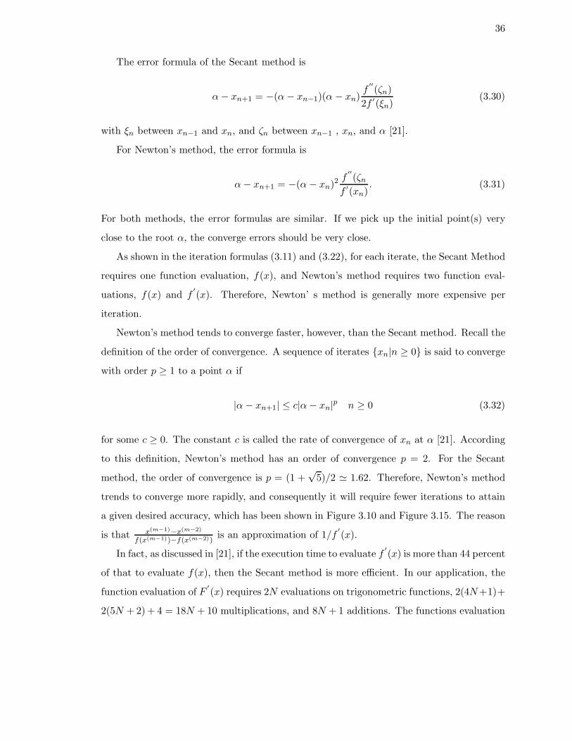
In fact, as discussed in [21], if the execution time to evaluate f′
(x) is more than 44 percent
of that to evaluate f(x), then the Secant method is more efficient. In our application, the
function evaluation of F′
(x) requires 2N evaluations on trigonometric functions, 2(4N+1)+
2(5N +2)+ 4 = 18N +10 multiplications, and 8N +1 additions. The functions evaluation

37
of F′′
(x) requires 2N evaluations on trigonometric functions, 2(5N + 2) + 2(6N + 2) +
12 = 26N + 20 multiplications, and 8N + 3 additions. Therefore, for the computation of
multiplications and additions, the ratios of evaluation are 26N+2018N+10 and 8N+3
8N+1 respectively.
Therefore, the Secant method tends to be more efficient in this application when N is large.
3.5 Approximate Maximum Likelihood Estimation using FFT
and Bisection Method
Although we have introduced two iterative ML estimators which can track the CRLB
over a wide range of SNR, both of them have a common drawback. Without the knowledge
of the observation, the estimator may pick up the points which are not close enough to
the peak. Therefore, in order to ensure the converge, we introduce another root-finding
method called the bisection method. If f is a continuous function on the interval [a, b] and
f(a)f(b) < 0, then the bisection method converges to the root of f by halving the range.
The best estimation is the midpoint of the smallest range found. Therefore, after n steps,
the absolute error is
|x(n) − x(n−1)| = |b− a|2n
.
In our application, we firstly use the coarse search to locate the peak index, k, of the
Fourier Transform observation. Then we initialize ω(0) = (k − 1)2π/(MT ) and ω(1) =
(k + 1)2π/(MT ). Since ω(0) and ω(1) locate on two opposite sides of ωbisection, which
maximizes F (x) approximately, we can ensure convergence. The stop conditions for the
FFT-bisection MLE is the same as those of the FFT-Secant MLE. The algorithm of the
bisection method is described in Algorithm 3.
Figure 3.18 and Figure 3.19 show the MSE of the frequency and phase estimators of the
FFT-bisection MLE respectively as a function of SNR for M = 210, M = 212, and M = 214,
for a complex observation. All the results assume an observation with N = 513, sampling
period T = 1 second, and the first sample time t0 = −256. The frequency and the phase
are independent random variables for the uniform distributions (3.6) and (3.7) respectively.
500 realization of the complex exponential signal using (2.1) and AWGN are generated with

38
Algorithm 3 The Bisection Method
Import ω(0), ω(1)
if F′
(ω(0)) ≤ 0 then
lo = ω(0)
hi = ω(1)
else
lo = ω(1)
hi = ω(0)
end if
ω(2) = lo+ (hi−lo)2
m = 2while (ω(m−1) 6= lo)AND(ω(m−1) 6= hi) dom = m+ 1if F
′
(ω(m−1)) ≤ 0 then
lo = ω(m−1)
else
hi = ω(m−1)
end if
∆ = hi−lo2
ω(m) = lo+∆if |∆| ≤ ε OR F
′
(ω(m−1)) == F′
(ω(m)) OR F′
(ω(m)) == 0 then
BREAKend if
end while
return ω(m)

39
fixed b0 = 1. The error tolerance ε is set to 10−4 for the iteration. The initial values are
ω(0) = (k − 1)2π/(MT ) and ω(1) = (k + 1)2π/(MT ), where k is the peak index estimated
by the coarse search.
−10 0 10 20 30 40 50 60
10−14
10−12
10−10
10−8
10−6
10−4
10−2
100
SNR(dB)
mea
n sq
uare
d fr
eque
ncy
estim
atio
n er
ror
M = 210
M = 212
M = 214
CRLB
ε2
Figure 3.18: Mean squared frequency estimation error for complex signal of FFT-bisectionMLE with ε = 10−4.
Compared with the FFT-Secant ML estimator and the FFT-Newton ML estimator, the
most obvious advantage of the FFT-bisection ML estimator is that the estimator converges
even with small values of M . As shown in Figure 3.18, the estimator with M = 210 can
track the CRLB over a small range of SNR. However, compared with the FFT-Secant and
the FFT-Newton estimators with the same value of M , the estimators with M = 212 and
M = 214 have worse performances. They can only track the CRLB up to a SNR about
9dB, which is a smaller estimation range. In order to improve the performance, we increase
ε from 10−4 to 10−6. As shown in Figure 3.20, the frequency estimation range is extended
to the SNR of 50dB. We try to increase ε further to 10−8. As shown in Figure 3.21, the
frequency estimation range extends to the SNR of 60dB.

40
−10 0 10 20 30 40 50 6010
−10
10−8
10−6
10−4
10−2
100
SNR(dB)
mea
n sq
uare
d ph
ase
estim
atio
n er
ror
M = 210
M = 212
M = 214
CRLB
Figure 3.19: Mean squared phase estimation error for complex signal of FFT-bisection MLEwith ε = 10−4.

41
−10 0 10 20 30 40 50 6010
−15
10−10
10−5
SNR(dB)
mea
n sq
uare
d fr
eque
ncy
estim
atio
n er
ror
M = 210
M = 212
M = 214
CRLB
ε2
Figure 3.20: Mean squared frequency estimation error for complex signal of FFT-bisectionMLE with ε = 10−6.

42
−10 0 10 20 30 40 50 60
10−14
10−12
10−10
10−8
10−6
10−4
10−2
100
SNR(dB)
mea
n sq
uare
d fr
eque
ncy
estim
atio
n er
ror
M = 210
M = 212
M = 214
CRLB
Figure 3.21: Mean squared frequency estimation error for complex signal of FFT-bisectionMLE with ε = 10−8.

43
Although decreasing the ε can improve the estimation accuracy, at the same time, the
execution time also increases. Compared with other two iterative estimators, the FFT-
bisection estimator has the slowest convergence speed. By using the definition of the order
of convergence (3.32) given in Section 3.4.1, we can find the order of convergence of the
bisection method is 1. It means the bisection converges linearly. Compared with other
two estimators, which converge quadratically, the FFT-bisection estimator does not have
advantage on convergence speed. Therefore, the bisection method is not the first choice.
When other two estimators do not converge, then we can apply the FFT-bisection MLE for
estimation because the convergence is guaranteed.
3.6 Conclusion
In this chapter, we discussed five approximate maximum likelihood estimators and anal-
ysed the their performance in terms of the mean squared frequency and phase estimation
errors as well as the computational complexity. Firstly, we introduced the Fast Fourier
Transform Maximum Likelihood Estimator (FFT MLE), which cannot track the CRLB at
high SNR unless the number of FFT points becomes very large. Then we presented four
fine search techniques, each of them uses the FFT MLE as the coarse search and refines
this coarse estimate to improve the performance. The first one is using the quadratic in-
terpolation to locate the approximate maximum, which has better estimation performance
but still cannot track the CRLB at the high SNR unless M is large. Then we provided a
detailed study about the FFT-Secant MLE, which is presented by Rife in [8]. After that,
we proposed other two iterative estimators: the FFT-Newton MLE and the FFT-bisection
MLE. We discussed the MSE of these three iterative MLE as well as the computational
complexity of them.
Besides the FFT-Secant MLE and the FFT-Newton MLE with bad initial values, all the
proposed FFT-based MLEs have similar threshold, which is about a SNR of -9dB. All of
them can attain the CRLB at low SNR. However, when the SNR is high, some MLEs fail to
achieve the CRLB. For a small value of M , the FFT MLE cannot achieve the CRLB at high
SNR values. Compared with the FFT MLE, the FFT-Quad MLE has a wider estimation

44
range. However, it only achieves the CRLB at 60dB when M = 214. For the iterative
MLEs, the FFT-Secant MLE and the FFT-Newton MLE do not converge when M = 210.
The reason is the initial points are not sufficiently close to the root of F′
(ω). When M is
larger, both FFT-Secant and FFT-Newton MLEs can attain the CRLB up to 60dB SNR
with reasonable error tolerance. The FFT-bisection MLE can always attain the CRLB at
60dB SNR because its algorithm guarantees the convergence.
For the estimation at low SNR, we recommend the user to choose the FFT MLE or
the Quad MLE with two reasons. The first reason is both MLEs can attain the CRLB at
low SNR. In addition, the computational complexity of the FFT MLE and the Quad MLE
is less than the iterative MLE because the function evaluation of F′
(ω) is not efficient.
For the estimation at high SNR, neither the FFT MLE nor the Quad MLE is a good fit
because both of them fail to achieve the CRLB at high SNR unless we use a large value of
M . Among the three iterative MLEs, we encourage the user to try the FFT-Secant MLE
at first. The FFT-Secant needs less computation than the FFT-Newton MLE and has
faster convergence speed than the FFT-bisection MLE. When the FFT-Secant MLE does
not converge, an alternative estimator is the FFT-bisection MLE, which can guarantee the
convergence.
We believe the these discussed methodologies will be useful in applications such as data
analysis and performance evaluation. Therefore, for a system with low sampling rate, the
proposed estimators can be applied to the real-time applications via hardware accelerating
such as Field-Programmable Gate Array (FPGA) and Graphics Processing Unit (GPU).
By using these devices, the most time consuming part, the computation of the FFT, can
be reduced significantly.

45
Chapter 4
Zero Crossing Phase and
Frequency Estimation
The common feature of the ML estimators presented in previous chapter is the estimator
requires to know the entire signal before doing estimation. However, in a real-time applica-
tion, this approach may lead to undesired latency in the computation of the estimates. In
real-time applications, it is desirable to estimate the unknown parameters in a sequential
way. This section presents a new low-complexity and low-latency algorithm for estimating
the phase and frequency of a single tone in white noise. The proposed “zero-crossing” (ZC)
phase and frequency estimator is based on zero-crossing detection of the real and imaginary
parts of the complex observation. Like Tretter and Kay estimators in [13] and [14], the ZC
estimator is based on the linear regression of the instantaneous phase of the observation of
(2.1). A key difference is that the ZC estimator operates only on the time/phase coordinates
of the real and imaginary zero crossings of (2.1). An advantage of this approach is that no
arctangent operations are required since the phase of the signal at zero crossings is known
(modulo 2π). Another advantage of this approach is that the number of zero crossing is
(2.1) is typically less than N . A sequential least squares implementation of the zero-crossing
estimator is also presented in which the phase and frequency estimates are updated as each
new crossing is detected. This feature provides the availability for real-time applications.

46
4.1 Algorithm
4.1.1 Zero-Crossing Phase and Frequency Estimator
The zero-crossing estimator operates by detecting zero crossings in the real and imagi-
nary components of (2.1) and storing the estimated time and phase of these zero crossing
points to a coordinate set S = (t1, φ1), . . . , (tL, φL) where L is the number of detected
zero crossings. The zero crossing occur at known phase (modulo 2π) according to Table
4.1. The ZC estimate is the obtained by performing linear regression on the coordinate set
S.
Table 4.1: Phase of a complex exponential at zero crossing
type of zero crossing phase
imag part, positive k2π
real part, negative k2π + π/2
imag part, negative k2π + π
real part, positive k2π + 3π/2
In order to avoid the incorrect zero crossing detection, which can be caused by the
noise, a state machine shown in Figure 4.1 is used to detect zero crossings. The variable
x[n] denotes either the real part or imaginary part of z[n]. A negative-slope zero crossing
is detected on state transitions 1 → 2 and 3 → 2. A positive-slope zero crossing is detected
on state transitions 2 → 1 and 4 → 1. The hysteresis parameter α ≥ 0 sets the threshold
at which zero crossings are detected. Two of these state machines run simultaneously, each
appending coordinates to S as zero crossings are detected in the real and imaginary parts
of the observation.
In order to illustrate how the state machine works, consider the example shown in Figure
4.2 with α = 0.5. We initialize the coordinate set S = ∅. The first zero crossing is detected
by the imaginary state machine as a positive-slope zero crossing of the imaginary part of
the signal when state of the imaginary signal transitions from state 4 to state 1 at sample
index n = 8. The time of this crossing is estimated by using a simple linear interpolation
between the last sample in state 2, i.e. n = 4, and the first sample in state 1, i.e. n = 8.

47
Figure 4.1: State machine implementation of the zero crossing detector.
0 5 10 15 20 25 30−1.5
−1
−0.5
0
0.5
1
1.5
sample index n
obse
rvat
ion
real partimaginary part
Figure 4.2: Noisy observation with α = 0.5.

48
Therefore, the time t1 is computed by (4.1)
t1 = tn1 −=z[n1]
=z[n2]−=z[n1]tn2−tn1
(4.1)
where tn1 = 4T , tn2 = 8T and =z[n] denotes the value of the imaginary part of the
complex exponential signal z[n] at sample index n. The phase of this positive-slope zero
crossing of the imaginary signal is set to zero. Hence, the first coordinate (t1, 0) is added
to the coordinate set S.The next zero crossing in Figure 4.2 is detected by the real state machine as a negative-
slope zero crossing of the real part of the signal when state of the real signal transitions
from state 3 to state 2 at sample index n = 12. The time of this zero crossing is estimated
by the simple linear interpolation between the last sample in state 1, i.e. n = 9, and the
first sample in state 2, i.e. n = 12. Therefore, the time t2 is computed by (4.2)
t2 = tn2 −<z[n2]
<z[n1]−<z[n2]tn1−tn2
(4.2)
where tn1 = 9T , tn2 = 12T and <z[n] denotes the value of the real part of the complex
exponential signal z[n] at sample index n. The phase of this negative-slope zero crossing of
the real signal is set to π/2 and the second coordinate (t2, π/2) is added to the coordinate
set S.This processing is repeated as additional zero crossings are detected by the real and
imaginary state machines. In the example shown in Figure 4.2, a total of five zero crossings
are detected. Therefore, S = (t1, 0), (t2, π/2), (t3, π), (t4, 3π/2), (t5, 2π). At any point in
time once L ≥ 2, the zero crossing phase and frequency estimates can be generated by
performing a linear regression [24] on S to determine the least-squares fit for the slope and
intercept. the stop and intercept are set to ωZC and θZC , respectively.
4.1.2 Sequential Implementation
Like other linear-regression-based estimators, such as Tretter’s method, the ZC estimator
also can be implemented efficiently on a sample-by-sample basis. Prior to the first sample

49
of the observation, we initialize the tracking variables A = B = C = D = E = 0. When
a new coordinate (ti, θi) is added to the coordinate set S, the tracking variables are also
updated as follows:
A = A+ t2i ,
B = B + 1,
C = C + ti
D = D − tiθi, and
E = E − θi (4.3)
As shown in [24], the intercept and slope can be calculated directly from the tracking
variables as
θZC = intercept = −EA− CD
BA− C2, and (4.4)
ωZC = slope = −C
AθZC − D
A. (4.5)
4.2 Computational Complexity
Since there are typically four real and imaginary zero crossings per period, the number
of real and imaginary zero crossings in (2.1) is approximated as L ' 4Nf0fs , where f0 = ω0
2π .
At each detection of zero crossing, the estimator calculates the time of the zero crossing
(via interpolation) and also updates the tracking variables. The simple linear interpolation,
as shown in (4.1) and (4.2), requires one real-valued multiplication and three real-valued
additions. The update of the tracking variables requires two real-valued multiplications and
five real-valued additions. Computing the intercept and slope in (4.4) and (4.5) requires
eight real-valued multiplications and five real-valued additions. Therefore, the total number
of multiplications required to implement the zero-crossing estimator can be approximated
as
number of real multiplication ' 3L+ 8 =12Nf0fs
+ 8, (4.6)

50
and
number of real addition ' 8L+ 5 =32Nf0fs
+ 5. (4.7)
Note that these operations (except for the last eight multiplications and the last five addi-
tions) can be performed as the sample arrives. Also, there are no arctangent operations,
which are typically performed with a lookup Table 4.2.
Table 4.2: Computational Complexity of Tretter, Kay, and zero-crossing estimators
Algorithm Number of real multiplication Number of arctangent
Zero-crossing 12Nf0fs +O(1) 0
Kay with exact atan2 5N +O(1) N − 1
Tretter with exact atan2 N +O(1) N
Kay with approx atan2 7N +O(1) 0
Tretter with approx atan2 3N +O(1) 0
For the approximations for the arctangent function were discussed in [25], each approx-
imate arctangent can be computed with one to three real-valued multiplications. In the
table above, we assume two real multiplications per arctangent operation. For the complex
multiplication, we use the fact that one complex multiplication is equal to four real-valued
multiplications.
4.3 Numerical Results and Discussion
This section presents numerical results comparing the proposed zero-crossing estimator
to Tretter’s and Kay’s estimators. For Tretter’s and Kay’s estimators, we use both the
exact arctangent and the approximate four quadrant arctangent [25].
Figure 4.3 and Figure 4.4 show the MSE of the frequency and phase estimators of the
zero-crossing estimator, Kay’s estimator, and Tretter’s estimator respectively as a function
of SNR for a complex observation. All the results assume an observation with N = 513,
sampling period T = 1 second, and the first sample time t0 = −256. The frequency is an
independent random variable for a uniform distribution
ω0 ∼ U(0.09 × 2π, 0.11 × 2π). (4.8)

51
The phase is an independent random variable for a uniform distribution
θ0 ∼ U(−π, π). (4.9)
500 realizations of the complex exponential signal using (2.1) and AWGN are generated
with fixed b0 = 1. The hysteresis parameter of the ZC estimator is α = 0.4. Since Tretter’s
method using the exact arctangent is as same as Kay’s method using the exact arctangent
[19], we use the same plot for these two methods.
−10 −5 0 5 10 15 20 25 30 35 4010
−12
10−10
10−8
10−6
10−4
10−2
100
SNR (dB)
mea
n sq
uare
d fr
eque
ncy
estim
atio
n er
ror
zero−crossingTretter/Kay with exact atan2Tretter with approx atan2Kay with approx atan2CRLB
Figure 4.3: Mean squared frequency estimation error of ZC estimator with α = 0.4.
Figure 4.3 shows the mean squared frequency estimation error as a function of SNR.
Besides Kay’s estimator with the approximate arctangent, all the estimators have the same
threshold, which is about a SNR of 10dB. The ZC estimator provides frequency within
about 2.5dB of the CRLB for 10 ≤ SNR ≤ 30dB. Above 30dB SNR, the ZC estimator’s
performance continues to improve, but deviates from the CRLB due to the error of linear
interpolation as discussed in [26]. Tretter’s estimator, independent of which method is used

52
−10 −5 0 5 10 15 20 25 30 35 4010
−8
10−7
10−6
10−5
10−4
10−3
10−2
10−1
100
101
SNR (dB)
mea
n sq
uare
d ph
ase
estim
atio
n er
ror
zero−crossingTretter/Kay with exact atan2Tretter with approx atan2Kay with approx atan2CRLB
Figure 4.4: Mean squared phase estimation error of ZC estimator with α = 0.4.
to calculate arctangent function, can always track the CRLB up to a SNR of 40dB. Kay’s
estimator with the approximate arctangent function fails to track the CRLB. The reason
is that the Kay estimator performs arctangent operations on the phase increments between
two consecutive samples of the observation. At high SNR the sequence of phase increments
tends to be very similar. Hence, any error in the arctangent approximation is repeated and
the frequency estimate becomes biased.
Figure 4.4 shows the mean squared phase estimation error as a function of SNR. The
threshold of all the estimators is about a SNR of 10dB. The ZC estimator tracks the CRLB
within about 2.5 dB up to a SNR of 30dB. After 30 dB, the ZC estimator’s performance
still improves but deviates from the CRLB due to the error of linear interpolation. Since
the phase estimator of Kay’s method depends on the estimated frequency, the phase plot of
the Kay’s method with approximate arctangent starts to deviate from the CRLB at 20dB.
Other estimators can track the CRLB up to a SNR of 40dB.
Figure 4.5 shows the frequency estimate MSE as a function of SNR with α = 0.2.

53
−10 −5 0 5 10 15 20 25 30 35 4010
−12
10−10
10−8
10−6
10−4
10−2
100
SNR (dB)
mea
n sq
uare
d fr
eque
ncy
estim
atio
n er
ror
zero−crossingTretter/Kay with exact atan2Tretter with approx atan2Kay with approx atan2CRLB
Figure 4.5: Mean squared frequency estimation error of ZC estimator with α = 0.2.
−10 −5 0 5 10 15 20 25 30 35 4010
−8
10−7
10−6
10−5
10−4
10−3
10−2
10−1
100
101
SNR (dB)
mea
n sq
uare
d ph
ase
estim
atio
n er
ror
zero−crossingTretter/Kay with exact atan2Tretter with approx atan2Kay with approx atan2CRLB
Figure 4.6: Mean squared phase estimation error of ZC estimator with α = 0.2.
54
Compared with Figure 4.3, the threshold is increased to 12.5dB. However, the gap between
the ZC estimator and the CRLB is smaller. For example, at 40dB, the ZC estimator with
α = 0.4 has a MSE about 7× 10⁻¹¹. At the same time, the ZC estimator with α = 0.2 has
a MSE about 2× 10⁻¹¹.
Figure 4.6 shows the phase estimate MSE as a function of SNR with α = 0.2. Compared
with Figure 4.4, the threshold is increases to 12.5dB. But the ZC estimator with α = 0.2
is closer to the CRLB. For example, at 40dB, the ZC estimator with α = 0.4 has a MSE
about 8× 10⁻⁷ in Figure 4.4. In Figure 4.6, the error is reduced to 5× 10⁻⁷.
In summary, when the hysteresis parameter α is reduced from 0.4 to 0.2, the threshold
of the estimation is increased. However, at the same time, the ZC estimator is closer to the
CRLB. Therefore, it is a trade-off to decide the value of the hysteresis parameter α.
4.4 Conclusion
This chapter proposes a new algorithm for the phase and frequency estimation of a single
tone complex observation in white noise. The proposed zero-crossing phase and frequency
estimator is based on the detection of zero crossing of the real and imaginary parts of the
complex observation and sequential least squares processing. Compared with other linear-
regression-based estimators, such as Tretter’s method and Kay’s method, the zero-crossing
estimator does not require any arctangent operations. In addition, the proposed estimator
provides low latency with the fact that phase and frequency estimates can be updated
sequentially as new zero crossings are detected.

55
Chapter 5
Zero Crossing Estimator
Refinements
The algorithm introduced in Section 4.1 is the fundamental algorithm of the zero-crossing
estimator. With some additional improvements and modifications, the performance of the
zero-crossing estimator can be improved significantly. In this section, three improvement
methods are introduced. The first refined estimator uses a new approach for interpolation
with better accuracy. The second approach uses a bandpass filter as the pre-processing. The
third approach uses the ZC estimator as the coarse search and the root-finding algorithm as
the fine search. For each new approach, we compute the mean squared frequency and phase
estimation errors as a function of SNR. Also, we compare the MSEs of the new approaches
with the fundamental approach. The numerical results show that all of the new approaches
have better performance.
5.1 Zero Crossing Estimator using Local Linear Regression
for Zero-crossings
Since the performance of the ZC estimator depends on the accuracy of the zero crossing
time estimates, the choice of the interpolation technique used to estimate the zero crossing
times is very important [26]. In Section 4.1.1, we discuss about using the simple linear

56
interpolation to estimate the time of crossing, i.e. (4.1) and (4.2). However, in this inter-
polation method, only two points are used. Hence, the accuracy of the interpolation is low.
A better interpolation method is proposed in this section.
In this new interpolation method, we use a local linear regression, which uses all of
the samples from the last sample above/below to the first sample below/above the hysteresis
threshold. Depending on the normalized frequency of the observation and the hysteresis
parameter, α, local linear regression can produce significantly better zero crossing time
estimates by exploiting the information contained in the samples between the hysteresis
thresholds.
Let’s recalled the example in Section 4.1.1, in order to estimate the time of the first zero
crossing by using this new method, we need to collect the sample indices and the associated
magnitudes and put into a coordinate set L. Therefore, when state machine of the imaginary
signal transitions from state 4 to state 1 at sample index n = 8, the coordinate set L is
L = (tn1 ,=z[n1]), (tn2 ,=z[n2]), (tn3 ,=z[n3]), (tn4 ,=z[n4]), (tn5 ,=z[n5]) (5.1)
where n1, n2, n3, n4, n5 are equal to 4, 5, 6, 7, 8 respectively, tni= ni × T , and =z[ni] is
the imaginary part of the complex exponential signal z[n] at sample index ni. Now we can
apply the linear regression to the coordinate set L. Since this regression can be achieved
on a sample-by-sample basis, we can use the similar idea presented Section 4.1.2. Five new
tracking variables, A, B, C, D, and E, are set and updated as shown in (4.3). After the zero
crossing is detected, the intercept, b, and the slope, g, are estimated by using (5.2) and
(5.3).
b = intercept = − EA− CD
BA− C2, and (5.2)
g = slope = − C
Ab− D
A. (5.3)
Then, the time of crossing is (5.4)
t = − b
g(5.4)

57
−10 −5 0 5 10 15 20 25 30 35 4010
−12
10−10
10−8
10−6
10−4
10−2
100
SNR (dB)
mea
n sq
uare
d fr
eque
ncy
estim
atio
n er
ror
zero−crossingTretter/Kay with exact atan2Tretter with approx atan2Kay with approx atan2CRLB
Figure 5.1: Mean squared frequency estimation error of ZC estimator via local linear inter-polation with α = 0.4.

58
−10 −5 0 5 10 15 20 25 30 35 4010
−8
10−7
10−6
10−5
10−4
10−3
10−2
10−1
100
101
SNR (dB)
mea
n sq
uare
d ph
ase
estim
atio
n er
ror
zero−crossingTretter/Kay with exact atan2Tretter with approx atan2Kay with approx atan2CRLB
Figure 5.2: Mean squared phase estimation error of ZC estimator via local linear interpo-lation with α = 0.4.

59
5.1.1 Numerical Results and Discussion
Figure 5.1 and Figure 5.2 show the mean squared frequency and phase estimation errors
as a function of SNR for a complex observation. The simulation parameters are the same
as what we used in Section 4.3. For the interpolation, we use the local interpolation on
all the samples between the last sample above/below and the first sample below/above the
hysteresis threshold. Then the zero crossing time can be estimated. In this simulation, the
hysteresis threshold is α = 0.4.
Compared with Figure 4.3 and Figure 4.4, the performance of the ZC estimator us-
ing the new interpolation method is improved significantly. These results show that the
zero-crossing estimator provides frequency and phase estimates within about one dB of the
CRLB for 10 ≤ SNR ≤ 30dB. Above 30dB SNR, the zero-crossing estimator’s performance
continues to improve, but deviates from the CRLB due to the error of interpolation. How-
ever, compared with Figure 4.3 and Figure 4.4, the improvement is significant. For example,
in Figure 4.3, the mean squared frequency estimation error at 40dB is about 7× 10⁻¹¹. For
the ZC estimator using the local interpolation technique, the error is reduced to a MSE
about 1× 10⁻¹¹.
5.2 Zero Crossing Estimator using Pre-Filtered Observation
In many communication and signal processing applications, the central frequency is
known by both transmitter and receiver. For example, under IEEE 802.11g standard,
we know the central frequency of each channel. Therefore, a bandpass filter can be pre-
computed and used as the pre-processing of estimation. Since the noise is filtered, the
detection of the zero crossing is more accurate. Consequently, the accuracy of the ZC
estimator is improved.
5.2.1 Numerical Results and Discussion
Figure 5.3 and Figure 5.4 show the mean squared frequency and phase estimate errors
as a function of SNR for a complex observation. All the results assume an observation with
N = 513, sampling frequency fs = 16000 Hz, and the first sample time t0 = −256. The

60
−10 −5 0 5 10 15 20 25 30 35 4010
−12
10−10
10−8
10−6
10−4
10−2
100
SNR (dB)
mea
n sq
uare
d fr
eque
ncy
estim
atio
n er
ror
zero−crossingTretter/Kay with exact atan2Tretter with approx atan2Kay with approx atan2CRLB
Figure 5.3: Mean squared frequency estimation error of ZC estimator with α = 0.4 and a64th order FIR filter.

61
−10 −5 0 5 10 15 20 25 30 35 4010
−7
10−6
10−5
10−4
10−3
10−2
10−1
100
101
SNR (dB)
mea
n sq
uare
d ph
ase
estim
atio
n er
ror
zero−crossingTretter/Kay with exact atan2Tretter with approx atan2Kay with approx atan2CRLB
Figure 5.4: Mean squared phase estimation error of ZC estimator with α = 0.4 and a 64thorder FIR filter.

62
frequency is an independent random variable for a uniform distribution
ω0 ∼ U(1019 × 2π, 1021 × 2π). (5.5)
The phase is an independent random variable for a uniform distribution
θ0 ∼ U(−π, π). (5.6)
500 realizations of the complex exponential signal using (2.1) and AWGN are generated
with fixed b0 = 1. The hysteresis parameter of the ZC estimator is α = 0.4. Simple
linear interpolation is used in this simulation. In addition, a 64th order Finite Impulse
Response (FIR) filter is used to pre-process the observation. Therefore, the observation will
be filtered by the FIR filter and the output of the filter will be used for the estimation. In
this simulation, the passband of the bandpass filter is [920, 1120] Hz.
Compared with Figure 4.3 and Figure 4.4, the performance of the ZC estimator is
improved significantly. In Figure 5.3 and Figure 5.4, the threshold is decreased from a SNR
of 10dB to a SNR of 0dB, which is better than that of Tretter and Kay estimators. In
addition, the frequency and phase estimates within about one dB of the CRLB up to a
SNR of 40dB, which is much better than the fundamental ZC estimator without filter.
5.3 Zero Crossing Estimator using Non-Linear Iterative Method
In Chapter 3, we presented five approximate maximum likelihood estimators. The FFT-
Secant MLE, the FFT-Newton MLE, and the FFT-bisection MLE use the Fast Fourier
Transform (FFT) as the coarse search and different root-finding algorithms as the fine
search. Compared with FFT MLE, the performance of these three MLEs are improved
significantly due to iterative methods. However, the computation of the FFT is slow and
the FFT estimators require to know the entire observation before estimation. Therefore, the
latency may be too high for real-time application. Nevertheless, these estimators provide a
new idea which uses the ZC estimator as the coarse search and the root-finding algorithm
as the fine search.

63
In this new approach, we still implement the zero-crossing estimator as we proposed
in Section 4.1. After computing (4.4) and (4.5), the estimated frequency ωZC are used
as the coarse search frequency estimate for the fine search. Then we can use the Secant
Method, as the fine search, to find the root of F′
(ω) in (3.18) because it has fast convergence
speed and needs less computation. In the example shown in Section 3.3, only two steps are
required to converge with error tolerance ε = 10−4. Now the initial values of the Secant
Method are ω(0) = ωZC and ω(1) = ωZC −∆ω, where ∆ω is a very small real number. As
shown in Figure 4.3, the error of ZC estimator is very small. Thus, we can ensure that the
initial points we pick are sufficiently close to the root. Consequently, we can ensure the
convergence of the iteration. One thing we should notice is that in this approach, we do not
need to compute the FFT. Therefore, the computational complexity of this new approach
is less than the FFT-based MLEs. The algorithm of the Secant Method is shown Algorithm
1. The converged value will be ωZC−Secant and finally we can compute θZC−Secant by using
(5.7)
θZC−Secant = ∠exp(−jωZC−Secantt0)A(ωZC−Secant). (5.7)
5.3.1 Numerical Results and Discussion
Figure 5.5 and Figure 5.6 show the mean squared frequency and phase estimation errors
as a function of SNR for a complex observation. All the results assume an observation
with N = 513, sampling period T = 1 second, and the first sample time t0 = −256. The
frequency is an independent random variable for a uniform distribution
ω0 ∼ U(0.09 × 2π, 0.11 × 2π). (5.8)
The phase is an independent random variable for a uniform distribution
θ0 ∼ U(−π, π). (5.9)
500 realizations of the complex exponential signal using (2.1) and AWGN are generated
with fixed b0 = 1. The hysteresis parameter of the ZC estimator is α = 0.4. The Secant

64
−10 −5 0 5 10 15 20 25 30 35 4010
−12
10−10
10−8
10−6
10−4
10−2
100
102
SNR (dB)
mea
n sq
uare
d fr
eque
ncy
estim
atio
n er
ror
zero−crossingTretter/Kay with exact atan2Tretter with approx atan2Kay with approx atan2CRLB
Figure 5.5: Mean squared frequency estimation error of ZC estimator via the Secant Methodwith α = 0.4.

65
−10 −5 0 5 10 15 20 25 30 35 4010
−8
10−7
10−6
10−5
10−4
10−3
10−2
10−1
100
101
SNR (dB)
mea
n sq
uare
d ph
ase
estim
atio
n er
ror
zero−crossingTretter/Kay with exact atan2Tretter with approx atan2Kay with approx atan2CRLB
Figure 5.6: Mean squared phase estimation error of ZC estimator via the Secant Methodwith α = 0.4.

66
Method is used as the post-processing of estimation. The error tolerance is ε = 10−4. The
initial values of the Secant Method are ω(0) = ωZC and ω(1) = ωZC − 5× 10⁻⁴.
Compared with Figure 4.3 and Figure 4.4, the zero-crossing estimator with non-iterative
method has much better performance. Although the threshold of estimation remains the
same, the new approach has smaller mean squared error. As shown in Figure 5.5 and Figure
5.6, the new approach tracks the CRLB up to a SNR of 40dB.
5.4 Conclusion
In this chapter, we propose three improved approaches for the zero-crossing estimator.
Compared with the mean squared frequency and phase estimation errors given in Figure
4.3 and Figure 4.4, all of the new approaches have better performance. Compared with
the fundamental zero crossing estimator in Section 4.1, the first approach uses a local
interpolation to improve the performance. Rather than using the two points to estimate
the zero crossing time, the new interpolation algorithm uses all the points between the last
sample above/below and the first sample below/above the hysteresis threshold to locate
the time of zero crossing via a local linear interpolation. The numerical results show that
the gap between the MSE and the CRLB is smaller than the fundamental estimator. The
second approach uses a filter to improve the SNR. In the example we demonstrated, a
64th order FIR bandpass filter is used to reduce the power of noise. The numerical results
show that compared with the fundamental approach and the ZC estimator with accurate
interpolation, the ZC estimator with filter has a smaller threshold and MSEs. The third
approach is using a root-finding algorithm as the fine search to improve the performance of
the fundamental estimator. Although the threshold of this new method remains the same
as the fundamental method, this approach has the least MSE among all the zero-crossing
estimation refinements. The numerical results show that the estimator tracks the CRLB
up a high SNR of 40dB.
Among all of the improvements, many common applications will benefit from the second
one, which is uses the filter to pre-process the samples as they arrive. As what we will be
discussed in the following chapter, this approach can be implemented in a sequential way

67
by using the circular buffer [27]. Although the ZC estimator with accurate interpolation
can be applied in a real-time application as well, the performance of this estimator is worse
than that of the one with filter. For the ZC estimator with non-linear iterative method,
although the number of iterations is low, the function evaluation of F′
(ω) is not efficient.
Also, this approach may fail without the prior knowledge about the SNR of communication
channel.

68
Chapter 6
A Software-Defined-Radio
Implementation of Time-Slotted
Round-Trip Carrier
Synchronization for Distributed
Beamforming via Zero-Crossing
Estimation
Transmit beamforming is an energy-efficient communication technique in which a trans-
mitter sends a beacon over two or more antennas and aligns the phases of the transmissions
across the antennas such as, after propagation, the signals combine constructively at the
intended direction [5]. The recent idea about achieving transmit beamforming has been
extended from a single antenna array to a network of cooperating single-antenna sources
which behave in a distributed fashion, which is described as the distributed beamforming.
Unlike conventional transmit beamforming, each single-antenna transmitter has its local
oscillator, which is independent from other source nodes and also imperfect. Therefore, in

69
order to achieve beamforming at the destination in the desired direction, the carrier phase
and frequency synchronization among the transmitter nodes is necessary [17].
In [28], the round-trip carrier synchronization algorithm was proposed for the carrier
synchronization of the distributed beamforming. This algorithm uses the equivalence of
round-trip propagation delays through a multihop chain of source nodes to achieve phase and
frequency synchronization [17, 28]. [17] and [20] show an experiment of implementing the
round-trip carrier synchronization by using software-defined radios (SDRs). The experiment
includes two-source synchronization and three-source synchronization in both wired channel
and acoustic channel. The hybrid Phase Locked Loop (PLL) is used for estimating unknown
parameters. A two-source round-trip model is shown in Figure 6.1.
Figure 6.1: Time-slotted round-trip carrier synchronization system with two source nodes.
As shown in Figure 6.1, the fundamental concept of this algorithm is that an unmod-
ulated carrier transmitted by the destination node and “bounced” around the clockwise
circuit will incur the same total phase shift as an unmodulated carrier transmitted by the
destination node “bounced” around the counter-clockwise circuit. In practice, the “bounc-
ing” of carrier can be performed actively by having each source estimated the unknown
parameters of the received beacon transmitted by other nodes. Then each source transmit-

70
ted a periodic extension of the signal received in a previous timeslot. Coherent combing
is achieved since the destination is receiving the sum of two carriers, modulated by the
common message, after they have propagated through circuits with identical phase shifts.
In the algorithm above, each node estimates the frequency and phase of the received
signal in a specific timeslot. In order to reduce the total time for synchronization, a fast
frequency and phase estimator is required for each timeslot. Therefore, a sequential estima-
tor satisfies such requirement. Hence, we implement the proposed zero-crossing phase and
frequency estimator in the time-slotted round-trip carrier synchronization and analyse the
performance of this estimator in a wired channel.
In our implementation, we will use the methodology for the two-source case in wired
channel discussed in [17]. The following sections will introduce the protocol of two source
nodes synchronization system. Then the specific timeslot schedule and the map of equip-
ment connection are given. In addition, the C functions of each key component of the
round-trip synchronization system are discussed. Finally, the test results will be analysed
and compared with the results from [17].
6.1 Two-Source Synchronization
As illustrated in [17], in a two-source system, there are four timeslots for the round-trip
synchronization protocol. Among them, the first three slots are used for synchronizing the
local oscillator of each node and the last slot is used for beamforming.
TS(0) : The destination node transmits the sinusoidal primary beacon to both source nodes.
Both source nodes estimate phase and frequency from their local observation, denoted
as θ0i and ω0i, respectively, at source node Si for i ∈ 1, 2.
TS(1) : Source node S1 transmits a sinusoidal secondary beacon to source node S2. This
secondary beacon is transmitted as a periodic extension of the beacon received in
TS(0). S2 estimates local phase and frequency from this received observation which
are denoted by θ12 and ω12, respectively.
TS(2) : Source node S2 transmits a sinusoidal secondary beacon to source node S1. This sec-

71
ondary beacon is transmitted as a periodic extension of the beacon received in TS(0),
with initial phase extrapolated from the phase and frequency estimates obtained by
S2 in TS(0). S1 generates local phase and frequency estimates from this observation
denoted as θ21 and ω21, respectively.
TS(3) : Both sources transmit simultaneously to the destination as a distributed beamformer.
The carrier frequency of each source is based on both local frequency estimates ob-
tained in the prior timeslots. The initial phase of the carrier at each source is ex-
trapolated from the local phase and frequency estimates from the secondary beacon
observation.
6.2 Experimental Methodology for Two-Source Test inWire-
Connected Channel
Each source node in the wired two-source time-slotted round-trip carrier synchroniza-
tion system is implemented by using one Taxes Instrument TMS320C6713DSK board at
a sampling frequency 16kHz. Besides the DSK boards, the experiment kit also includes
a CD player (SONY CD Walkman D-CJ01), a Behringer EURORACK UB1201 Mixer, a
Tektronix TDS 3014 oscilloscope, a Marntz PMD 661 solid state recorder, various RCA,
BNC connectors, and cables for connecting between the electronic computers’ inputs and
outputs. The whole system is shown in Figure 6.2.
According to the discussion in Section 6.1, after the estimation, each source node needs
to keep its estimates for transmission. Therefore, we put the estimates in holdover. In
addition, each node needs to estimate the unknown parameters twice in the two-source
system. Therefore, we set two estimators and two holdovers on each node and they can
operate simultaneously.
The detector for the first beacon, the round-trip protocol, and the ZC estimator are
implemented by programming the TMS320C6713DSK in C language using Texas Instru-
ment’s Code Composer Studio integrated development environment. Each source node runs
the system independently and there is not connection between each two nodes. The “des-

72
Figure 6.2: Implementation block diagram of the two-source time-slotted round-trip carriersynchronization system where the blue and green lines each represents a different signalwired path

73
tination node” was created by using the CD player for playing primary beacon, as well as
the recorder for recording the beacons. An oscilloscope was connected to the output of the
recorder for real-time monitoring. Each test is a complete execution of the 4 timeslots of the
round-trip protocol. At the beginning, each source node enters into a state where it waits
for the primary beacon. Once the primary beacon is detected, the nodes start to execute
the round-trip protocol according to the schedule shown in Table 6.1.
Timeslot Time S1 S2
TS0
0.00s detect primary beacon detect primary beacon0.00-0.10s wait wait0.10-0.60s update tracking variables of ZC1 update tracking variables of
ZC10.6s estimate frequency and phase for ZC1 estimate frequency and phase
for ZC10.60-1.25s holdover ZC1 holdover ZC1
TS1
1.25-1.35s transmit holdover ZC1 holdover ZC11.35-1.85s transmit holdover ZC1 holdover ZC1 and update track-
ing variable of ZC21.85s transmit holdover ZC1 estimate frequency and phase
for ZC2 and holdover ZC11.85-2.25s transmit holdover ZC1 holdover ZC1 and ZC22.25-2.50s wait holdover ZC1 and ZC2
TS2
2.50-2.60s wait transmit holdover ZC1; alsoholdover ZC2
2.60-3.10s update tracking variables of ZC2 transmit holdover ZC1; alsoholdover ZC2
3.10 estimate frequency and phase for ZC2 transmit holdover ZC1; alsoholdover ZC2
3.10-3.50s holdover ZC2 transmit holdover ZC1; alsoholdover ZC2
3.50-3.80s holdover ZC2 holdover ZC2
TS33.80-5.80s transmit holdover ZC2 transmit holdover ZC25.80-6.80s clear state clear state6.80s re-arm primary beacon detector re-arm primary beacon detector
Table 6.1: Two-source round-trip synchronization protocol timing. After detection of theprimary beacon, each node keeps time using its sample clock running at 16 kHz.

74
6.3 Zero-Crossing Estimator Implemented on Source Node
The round-trip protocol and the ZC estimator are implemented on the TMS320C6713DSK
board via C language. Based on the architecture and the design of the TMS320C6713DSK
board, when a new sample arrives, the interrupt service routine (ISR) will be executed [29].
Therefore, the number of execution is equal to the sampling frequency in one second. In
order to implement the sequential estimation, all the C codes are included in the ISR. Be-
cause of two estimators and two holdovers, all the estimation variables, such as the tracking
variables and the estimates, are stored in array and indicated by the index of the estimator.
The following parts will give detailed discussion of the implementations of the round-trip
time table, the FIR filter, and the zero-crossing estimator. The competed code is presented
in Appendix.
6.3.1 Implementation of the Round-Trip Time Table
According to Table 6.1, the two-source round-trip synchronization protocol is divided
into four timeslots. There is a global variable called TS, which is used to identify the
timeslot. Since the ISR is executed when a new sample is arrived, in each time slot, we
use a unsigned integer counter to track the time. The variable counter is increased by one
when the ISR is executed. The time of each event is pre-loaded and we compare counter
with the pre-loaded schedule in each ISR call. Once they are equal, we will change to next
event. Here is an example of how to implement it in Time Slot 0 (TS0).
1
2 // de f i n e time f o r each event
3
4 const unsigned int s t a r t s l o t = 0 ; // s t a r t o f time s l o t
5 const unsigned int s t a r t l i s t e n = 1600; // s t a r t to l i s t e n @ 0.1 s
6 const unsigned int s t o p l i s t e n = 9600; // s top to l i s t e n @ 0.6 s
7 const unsigned int end s l o t = 20000; //end o f time s l o t @ 1.25 s
8 const unsigned int s t a r t p l a y = 0 ; // s t a r t to p lay
9 const unsigned int s top p lay = 16000; // s top to p lay @ 1s

75
10
11 //end
12
13 // schedu l e p ro t o co l
14 i f ( ( counter < s t a r t l i s t e n )&&(counter>=s t a r t s l o t ) ) // 0.1 s wai t
15 16 // wai t
17 counter++;
18 19 // 0.5 s t rack
20 else i f ( ( counter >= s t a r t l i s t e n )&&(counter < s t o p l i s t e n ) )
21 22 // update t r a c k i n g v a r i a b l e f o r ZC1
23 counter++;
24
25 26 else i f ( counter == s t o p l i s t e n )
27 28 // es t imate f requency and phase f o r ZC1
29
30 counter++;
31 phase updater ( 0 ) ;
32 33 else i f ( ( counter > s t o p l i s t e n ) && ( counter < end s l o t ) )
34 35 // ho ldove r ZC1
36 counter ++;
37 38 else i f ( counter == end s l o t )

76
39 40 // ho ldove r ZC1
41 TS++; // change to next time s l o t
42 counter = 0 ;
43
6.3.2 Implementation of Zero-Crossing Estimator
The implementation of zero crossing estimator includes four part: the state machine,
the interpolation, the update of tracking variables, and the estimation based on tracking
variables. The first three components are implemented sequentially. They are executed
when a new sample arrives. The last component, the estimation, is only called at 0.6
second.
Implementation of State Machine
As discussed in Section 4.1, each received sample will be sent to the state machine and
compared with the hysteresis parameter α. Since the transmitted beacon is sinusoid signal,
therefore, only one state machine is needed. We use the if-else statement to implement the
state machine. Once the zero crossing is detected, the time and the phase will be generated
at first based on Table 4.1. Then the tracking variables will be updated according to (4.3).
Here is an example of showing the State 3 in C code.
1 i f ( s t a t e [ZCnum] == 3)
2 3 i f ( input > A)
4 5 // t r an s i t i o n to s t a t e 1
6 7 else i f ( ( input > A i ) && ( input < A))
8 9 // s tay in s t a t e 3

77
10 11 else i f ( input < A i )
12 13 // d e t e c t zero−c ro s s i n g
14
15 // compute time and phase v ia
16 // s imple l i n e a r i n t e r p o l a t i o n
17
18 // update the t r a c k i n g v a r i a b l e s
19 // t r an s i t i o n to s t a t e 2
20
21 22
Implementation of Simple Linear Interpolation
In order to estimate the time of zero crossing, we implement the simple linear interpo-
lation on the last sample above the upper hysteresis parameter and the first sample below
the lower hysteresis parameter, which has been presented in Section 4.1. In the software
implementation, we use two variables to track these two samples. Once a zero crossing is
detected, we apply either (4.1) or (4.2) to estimate the time. The phase of the zero crossing
is decided according to Table 4.1. Here is an example of showing linear interpolation in
State 3.
1
2 // I n t e r p o l a t i o n
3 s l op e = ( i 2 v a l u e [ZCnum] − i 1 v a l u e [ZCnum] ) ∗ f s ;
4 temp = i2 [ZCnum] − i 1 [ZCnum] ;
5 s l op e = s l op e / (double ) ( temp ) ;
6 zt [ZCnum] = (double ) i 1 [ZCnum]∗ i n v f s ;
7 zt [ZCnum] = zt [ZCnum] − i 1 v a l u e [ZCnum]/ s l op e ;

78
8 //END of i n t e r p o l a t i o n
9
10 n [ZCnum]++; // update number o f zero c ro s s i n g s
11
12 //Decide phase
13 i f (n [ZCnum]>=2)
14 15 ph [ZCnum] = ph [ZCnum] + pi ;
16 17 else ph [ZCnum] = pi ;
18
19
20 // s h i f t to s t a t e 2
21 s t a t e [ZCnum]= 2 ;
Implementation of Updating Tracking Variables
The tracking variables are initialized to zero before starting the estimation process. In
the process, the tracking variables are updated when a zero crossing is detected. Then the
tracking variables will be updated according to (4.3). Here is a C function for updating
tracking variables.
1 void ZC updatepar (unsigned short ZCnum)
2 3 AA[ZCnum] = AA [ZCnum]+ zt [ZCnum]∗ zt [ZCnum] ;
4 BB[ZCnum]++;
5 CC[ZCnum] = CC[ZCnum] + zt [ZCnum] ;
6 DD[ZCnum] = DD[ZCnum] − zt [ZCnum]∗ ph [ZCnum] ;
7 EE[ZCnum] = EE[ZCnum] − ph [ZCnum] ;
8

79
Implementation of Frequency and Phase Estimation
After receiving 0.5 second beacon, the frequency and phase estimates are computed
based on the tracking variables. (4.4) and (4.5) are used to estimate the frequency and
phase. The C code for estimating unknown parameters is listed as:
1 void ZC est imation (unsigned short ZCnum)
2 3 d e l t a [ZCnum] = BB[ZCnum]−CC[ZCnum]∗CC[ZCnum]/AA[ZCnum] ;
4 phhat [ZCnum] = −(EE[ZCnum]−CC[ZCnum]∗DD[ZCnum]/AA[ZCnum] )
5 / d e l t a [ZCnum] ;
6 fhat [ZCnum] = −CC[ZCnum]/AA[ZCnum]∗ phhat [ZCnum]−7 DD[ZCnum]/AA[ZCnum] ;
8
6.3.3 Implementation of Holdover
For each node, the a sinusoid beacon is generated based on the estimates and transmitted
to other nodes. As we discussed before, the transmitted beacon is a periodic extension of
the received beacon. Therefore, the phase, φ = ωnT + θ, is a large number since n is large.
In order to avoid overflow of using the C standard math function sin, we need to keep φ
within the range [0, 2π]. Hence, the unwrapping algorithm is needed. However, it is not
efficient to unwrap a large φ. Thus, we unwrap the phase φ under holdover mode. The
listing below shows the C function for updating phase in holdover mode.
1 void phase updater (unsigned short ZCnum)
2 3 phase [ZCnum] = phase [ZCnum] + fhat [ZCnum]∗ i n v f s ;
4
5 // phase unwrap
6 while ( phase [ZCnum] > 2∗ p i )7 phase [ZCnum] = phase [ZCnum] − 2∗ p i ;8 while ( phase [ZCnum] < 0)

80
9 phase [ZCnum] = phase [ZCnum] + 2∗ p i ;10
6.3.4 Implementation of FIR Filter
For the FIR bandpass filter, we use the Matlab to compute the filter coefficients and
pre-load them to the DSK. The discrete-time convolution is
y[n] =∞∑
k=−∞
x[k]h[n − k] (6.1)
where y[n] is the output of a linear, time-invariant, discrete-time system (LTI), x[n] is the
input, and h[n] is the unit pulse response. By using the circular buffers, we can implement
this convolution in sequence [27]. Here is an example of implementing the FIR filter via the
circular buffers.
1 /∗ ∗∗∗∗∗∗∗∗∗∗∗∗∗∗∗∗∗∗FIR F i l t e r ∗∗∗∗∗∗∗∗∗∗∗∗∗∗∗∗∗∗∗∗∗∗∗ ∗/2
3 i f ( cont == BL)
4 cont= 0 ;
5
6 // wr i t e s data in r i g h t channel i n t o b u f f e r
7 f i l t e r [ cont ] = read ing ;
8
9 j = 0 ;
10 input = 0 ;
11
12 for ( i = cont ; i>= 0 ; i−−)13 14 input += B[ j ]∗ f i l t e r [ i ] ;
15 j++;
16

81
17
18 for ( i = BL−1; i>cont ; i−−)19 20 input += B[ j ]∗ f i l t e r [ i ] ;
21 j++;
22
In the example above, array B stores the filter coefficients, BL is the order of filter, and
array filter with size BL stores the last BL received samples.
6.4 Data Analysis Methodology
As discussed in [17], the round-trip synchronization system has multipath channels.
Therefore, each source node should delay tracking the beacon until the transient effects of
the channel have become negligible. Then, during the steady-state portion of the observa-
tion, the source node starts the tracking process and sends the received samples to the state
machine for zero crossing detection. The estimates are put into holdover mode prior to the
end of the steady-state portion of the beacon. This is illustrated in Figure 6.3.
beacon
detected
ZC estimation
begins
ZC estimation ends
(holdover)
transient transient
envelop of beacon
steady-state
Figure 6.3: Effect of multipath on ZC estimation and holdover.
For the experiment with N wired beamforming tests, the uncompressed .wav recording

82
of the experiment was transferred to a PC and analysed in MATLAB to generated the
statistical results. The “power ratio” ρ of the beamformer is calculated by estimating the
power received during beamforming [17]. A power ratio of one means an ideal beamformer
without any frequency offset and phase offset. A power ratio of zero corresponds to the
case where the carriers completely cancel at the destination. In two source nodes system,
the formula for computing power ratio is
ρ[n] =
(
bbf0 [n]
b120 [n] + b210 [n]
)2
. (6.2)
The amplitude estimates in each test are obtained via the FFT-Secant MLE described in
Section 3.3.
6.5 Experimental Results
Three wired-channel experiments were performed and the experimental results can be
founded in Table 6.2. In this test, the central frequency of the beacon is 1020Hz. The
Variable Experiment 1 Experiment 2 Experiment 3
Min(ρ) 0.9996 0.9995 0.9990Max(ρ) 1.0000 1.0000 1.0000Mean(ρ) 0.9998 0.9998 0.9997Std(ρ) 7.5866e − 5 1.1948e − 4 2.2029e − 4
Table 6.2: Experimental results of two-source wired-channel tests. Each experiment con-sisted of 100 distributed beamforming tests.
sampling frequency is 16000Hz. For the zero-crossing estimator, the hysteresis parameter is
0.2. A bandpass FIR filter with 64 orders is used. The passband of the filter is [920, 1120]Hz.
The filter coefficients are generated by Matlab. Each experiment contains 100 tests.
Compared with the proposed experimental results in [17], our proposed estimator has
much better results. The minimum and mean of the power ratios are larger than those of
the PLL estimator. In addition, our power ratio is more consistent. The worst case of ZC
estimator is still 10 times better than the best case of PLL estimator.

83
Chapter 7
Conclusion
In the first part of this thesis we discussed two classes of maximum likelihood esti-
mation. The first category discussed is FFT-based maximum likelihood estimation (FFT
MLE). We based our discussion on the FFT MLE given by Rife and Boorstyn in [8]. The
numerical results show that their estimator can only achieve the CRLB at 60dB SNR with
a large value of M . In order to reduce the computational complexity, we proposed and dis-
cussed four refined approximate maximum likelihood estimators, the FFT-Quad estimator,
the FFT-Secant estimator, the FFT-Newton estimator, and the FFT-bisection estimator.
The numerical results show that for the small value of M , all the refinements can provide
better performance. Also, the refinements can achieve the CRLB at 60dB SNR with less
computational complexity.
The second part of this thesis proposed a new linear-regression-based maximum likeli-
hood estimator called the Zero-Crossing Phase and Frequency Estimator. Compared with
the well-known estimators in this category, Tretter’s estimator [13] and Kay’s estimator
[14], our proposed estimator has similar performance. In addition, the computational com-
plexity of our approach is less than the others for two main reasons. First, instead of using
every received sample, our approach only uses the zero crossings. Second, our approach
avoids the arctangent operation since the phase of each zero crossing is known. The re-
finements of the zero-crossing estimator show better performance than that of Tretter’s
and Kay’s estimators. Finally, our estimator is implemented in the time-slotted round-trip

84
carrier synchronization system of distributed beamforming using software-defined-radios.
Compared with the published results in [17], which use the hybrid Phase Lock Loop as the
estimator, our estimator has better and more consistent results.
There are many potential future research opportunities that stem from this thesis. One
such opportunity improves the accuracy of interpolation. Although both the simple inter-
polation and the local linear regression have given a good performance, at high SNR, the
error of interpolation causes the mean squared errors to deviate from the CRLB. Therefore,
a more accurate algorithm is needed to find the time of each zero crossing.

85
Appendix A
The Specification of Computer and
Matlab for Simulation
A.1 The Specification of Computer for Simulation
Table A.1: The Specification of simulation computer
Operation System (OS) 32-bit Microsoft Windows 7 Enterprise
Processor Two Intel(R) Core(TM) i7 870 processors with 2.93GHz
Number of Threads 8
Memory 4GB
A.2 The Specification of Matlab Software for Simulation
Table A.2: The Specification of Matlab
Version 7.11.0.584 (32-bit)
Maximum Possible Array 1249MB
Memory Available for All Arrays 1417MB

86
Appendix B
Source Code of the TMS320C6713
Source Node in the Two-Source
System
The following C code is the software implementation of the two-source time-slotted
round-trip carrier synchronization system. When the switch 1 on the board is pressed, the
DSK board performs as source node 1, whereas switch 2 corresponds to source node 2.
1 /* z_c.c by Yizheng Liao 12-OCT -2010 */
2
3 /*
4 This program is used to implement the two -source time -slotted
5 round -trip carrier synchronization system. The C code is loaded to
6 TMS320C6713 Digital Signal Processing Kit (DSK ). When the switch 1
7 on the DSK is pressed , the board performs as source node 1. When
8 switch 2 is pressed , the board performs as source node 2.
9 */
10
11 /* Defines */
12 #define CHIP_6713 // define the chip
13 #define thresh 0.2 // hysteresis parameter
14 #define bz 80 // size of detector buffer
15 #define N 2 // Number of node

87
16 #define PI 3.141592654 // phi
17
18 /* Header Files */
19 #include <stdio.h>
20 #include <stdlib.h>
21 #include <math .h>
22 #include <c6x.h>
23 #include <csl.h>
24 #include <csl_mcbsp .h>
25 #include <csl_irq.h>
26
27 // DSK Configuration Files
28 #include "dsk6713.h"
29 #include "dsk6713_aic23 .h"
30 #include "fastrts67x .h"
31
32
33 // contains coeff of filter
34 #include "FIRcoeff .h"
35
36 extern const int BL;
37 extern const double B[65];
38
39 /* Codec Configurations */
40 DSK6713_AIC23_CodecHandle hCodec;
41 // Codec configuration with default settings
42 DSK6713_AIC23_Config config = DSK6713_AIC23_DEFAULTCONFIG;
43
44
45
46
47 /* ******** Global constant ************** */
48
49 /* *************** Time Table for Each Time Slot ****************** */
50 /* For TS0 , TS1 , TS2 */
51
52 // start of time slot

88
53 const unsigned int start_slot = 0;
54
55 // start to listen @ 0.1s
56 const unsigned int start_listen = 1600;
57
58 // stop to listen @ 0.6s
59 const unsigned int stop_listen = 9600;
60
61 // end of time slot @ 1.25 s
62 const unsigned int end_slot = 20000;
63
64 // start to play
65 const unsigned int start_play = 0;
66
67 // stop to play @ 1s
68 const unsigned int stop_play = 16000;
69
70 /* For TS3 */
71
72 // start of time slot
73 const unsigned int start_slot_last = 0;
74
75 // wait 0.05 s before playing
76 const unsigned int start_play_last = 800;
77
78 // 160800; // play 10s
79 const unsigned int stop_play_last = 32800;
80
81 // 180000;
82 const unsigned int end_slot_last = 48800;
83 // wait 1.2s for end of time slot
84
85 const double pi = PI;
86 const double fs = 16000.00; // sampling frequency
87 const double A = thresh;
88 const double A_i = -thresh;
89 const double max = 32767;

89
90 const double det_sum = 0.01; // threshold for signal detector
91
92
93 /* Global Variables and Initializations */
94
95 /* FOR each Zero -Crossing estimator */
96
97 // threshold index
98 unsigned int i1[N], i2[N];
99
100 // sample asscoiated to threshold index
101 double i1_value [N], i2_value [N];
102
103 // tracking variables
104 double AA[N], BB[N], CC[N], DD[N], EE[N],delta[N];
105
106 // zero corssing time and phase
107 double zt[N], ph[N];
108
109 // observation index , state of state machine
110 unsigned int n[N], ind[N], state[N];
111
112 // estimates
113 double fhat [N], phhat[N];
114
115 // max of input beacon
116 double peak [N];
117
118 //1/ peak
119 double scale[N];
120
121 /* FOR FIR Filter */
122
123 // Buffer for filter count
124 unsigned int cont ;
125
126 // buffer for filter , size 65

90
127 double filter [65];
128
129 /* FOR Detector */
130
131 // 0.5 ms for detection
132 double detect_buffer [bz];
133
134 // detection index
135 int detector_index ;
136
137 // sum of detection
138 double detector_sum = 0;
139
140
141 /* Other Parameters */
142 double inv_max ;
143 unsigned int counter;
144 unsigned int start;
145 double inv_fs;
146 unsigned short TS;
147 unsigned short node ;
148 double acme ;
149
150 /* Functions */
151 interrupt void serialPortRcvISR (void );
152 void ZC_track (double input , unsigned short ZCnum);
153 void ZC_updatepar (unsigned short ZCnum);
154 void ZC_init (unsigned short ZCnum);
155 void ZC_estimation (unsigned short ZCnum);
156 double ZC_play (unsigned short ZCnum);
157 void phase_updater (unsigned short ZCnum);
158
159 void main ()
160
161 int i = 0;
162
163 DSK6713_init (); // Initialize the board support library

91
164 DSK6713_DIP_init (); // Initializes DIP switches
165 DSK6713_LED_init (); // Initializes LEDs
166
167 hCodec = DSK6713_AIC23_openCodec(0, &config ); // Open the codec
168
169 // Configure buffered serial port for 32-bit operation
170 // This allows transfer of both right and left channels
171 // in one read /write
172 MCBSP_FSETS (SPCR1 , RINTM , FRM );
173 MCBSP_FSETS (SPCR1 , XINTM , FRM );
174 MCBSP_FSETS (RCR1 , RWDLEN1 , 32 BIT);
175 MCBSP_FSETS (XCR1 , XWDLEN1 , 32 BIT);
176
177 // set the sampling rate
178 DSK6713_AIC23_setFreq (hCodec , DSK6713_AIC23_FREQ_16KHZ);
179
180
181 // Initialize right and left channel buffers with zeros
182 // So no garbage is in the channel buffers
183 for (i = 0; i < BL; i++)
184
185 filter[i] = 0;
186
187
188
189
190 for (i = 0; i < bz; i++)
191
192 detect_buffer [i] = 0.0;
193
194
195
196
197 inv_max =1 / max;
198 inv_fs = 1/ fs;
199 ZC_init (0);
200 ZC_init (1);

92
201 start = 0;
202 detector_index = 0;
203 detector_sum = 0;
204 counter = 0;
205 cont = 0;
206 acme = 0;
207
208
209 // Globally disables interrupts
210 IRQ_globalDisable ();
211 // Enables the NMI interrupt
212 IRQ_nmiEnable ();
213 // Maps an event to a physical interrupt
214 IRQ_map (IRQ_EVT_RINT1 , 15);
215 // Enables the event
216 IRQ_enable ( IRQ_EVT_RINT1 );
217 // Globally enables interrupts
218 IRQ_globalEnable ();
219
220 // decide the node number
221 if (DSK6713_DIP_get (1) == 0)
222
223 node = 1;
224
225 else if ( DSK6713_DIP_get (2) == 0)
226
227 node = 2;
228
229 else node = 0;
230 DSK6713_LED_on (node );
231
232 // Infinite Loop
233 while (1)
234
235
236
237

93
238
239
240 interrupt void serialPortRcvISR ()
241
242 union Uint32 combo; short channel [2]; data ;
243 short i = 0, j;
244 double input = 0;
245 double output = 0;
246 double reading ;
247 /* ***********************************Read input sample *************************/
248 // Read L+R channels
249 data .combo = MCBSP_read ( DSK6713_AIC23_DATAHANDLE);
250 reading = (double)data .channel [0]* inv_max ;
251 if (acme < reading )
252 acme = reading;
253
254
255
256 /* ******************************FIR Filter ************************/
257
258 if (cont == BL)
259 cont = 0;
260
261 // writes data in right channel into buffer
262 filter[cont ] = reading ;
263
264 j = 0;
265 input = 0;
266
267 for (i = cont; i>= 0; i--)
268
269 input += B[j]* filter[i];
270 j++;
271
272
273 for (i = BL -1;i>cont ;i--)
274

94
275 input += B[j]* filter[i];
276 j++;
277
278
279 cont ++;
280
281 /* ******************************FIR Filter END ***********************/
282
283
284 if (start == 0)
285
286
287 /* *********************************DETECTOR ********************* */
288
289 detect_buffer [ detector_index ] = input*input;
290
291
292
293
294 if (detector_index < 79)
295
296 detector_sum = detector_sum +
297 detect_buffer [detector_index ] -
298 detect_buffer [detector_index +1];
299 detector_index ++;
300
301 else
302
303 detector_sum = detector_sum +
304 detect_buffer [detector_index ] -
305 detect_buffer [0];
306 detector_index = 0;
307
308
309
310
311 if ( detector_sum > det_sum )

95
312
313 counter = 0;
314 start = 1;
315 ZC_init (0);
316 ZC_init (1);
317 TS = 0;
318
319
320
321
322 /* *********************************DETECTOR END ********************* */
323
324 /* *****************************State Machine ************************/
325 else
326
327 if(TS == 0) // time slot 0
328
329 if (( counter <start_listen )&&( counter >= start_slot )) // 0.1s wait
330
331 if (counter < 80)
332
333 detect_buffer [counter] = 0;
334
335 if (input > peak [0])
336
337 peak [0] = input;
338 scale [0] = 1/ peak [0];
339
340 counter ++;
341
342 else if (( counter >= start_listen ) && (counter < stop_listen ))
343 // 0.5s track
344
345 ZC_track (input ,0);
346 counter ++;
347 // ind [0]++;
348

96
349
350 else if (counter == stop_listen )
351
352 ZC_estimation (0);
353 counter ++;
354 ind [0]++;
355
356 else if (( counter > stop_listen ) && (counter < end_slot ))
357
358 ind [0]++;
359 counter ++;
360
361 else if (counter == end_slot )
362
363 ind [0]++;
364 TS ++;
365 counter = 0;
366
367
368 else if (TS == 1) // time slot 1
369
370 if (node == 1)
371
372 if (( counter >= start_play ) && (counter <= stop_play ))
373
374
375 output = ZC_play (0);
376 data .channel [0] = (short)( output *32000);
377 data .channel [1] = data .channel [0];
378 counter ++;
379 ind [0]++;
380 phase_updater (0);
381
382 // Write L+R channels
383 MCBSP_write ( DSK6713_AIC23_DATAHANDLE , data .combo );
384
385 else if (( counter > stop_play ) && (counter < end_slot ))

97
386
387 counter ++;
388
389 else if (counter == end_slot )
390
391 counter = 0;
392 TS ++;
393
394
395 else if (node == 2) // time slot 2
396
397 if (( counter <start_listen )&&( counter >= start_slot ))
398 // 0.1s wait
399
400 if (input > peak [1])
401
402 peak [1] = input;
403 scale [1] = 1/ peak [1];
404
405 counter ++;
406 ind [0]++;
407 phase_updater (0);
408
409 else if (( counter >= start_listen ) && (counter < stop_listen ))
410 // 0.5s track
411
412 ZC_track (input ,1);
413 counter ++;
414 ind [0]++;
415 phase_updater (0);
416
417
418 else if (counter == stop_listen )
419
420 ZC_estimation (1);
421 counter ++;
422 phase_updater (0);

98
423 phase [1] = (double)ind [1]* inv_fs*fhat [1] + phhat [1];
424 phase [1] = phase [1] - 2*pi *510;
425 while (phase [1] > 2*pi)
426 phase [1] = phase[1] - 2*pi;
427 while (phase [1] < 0)
428 phase [1] = phase[1] + 2*pi;
429 phase_updater (1);
430 ind [0]++;
431 ind [1]++;
432
433 else if (( counter > stop_listen ) && (counter < end_slot ))
434
435 ind [0]++;
436 ind [1]++;
437 counter ++;
438 phase_updater (0);
439 phase_updater (1);
440
441
442 else if (counter == end_slot )
443
444 phase_updater (0);
445 phase_updater (1);
446 ind [0]++;
447 ind [1]++;
448 TS ++;
449 counter = 0;
450
451
452
453
454
455 else if (TS == 2) // time slot 2
456
457 if(node == 1)
458
459 if (( counter <start_listen )&&( counter >= start_slot ))

99
460 // 0.1s wait
461
462 if (input > peak [1])
463
464 peak [1] = input;
465 scale [1] = 1/ peak [1];
466
467 counter ++;
468
469 else if (( counter >= start_listen ) && (counter < stop_listen ))
470 // 0.5s track
471
472 ZC_track (input ,1);
473 counter ++;
474
475
476 else if (counter == stop_listen )
477
478 ZC_estimation (1);
479 counter ++;
480 ind [1]++;
481
482 phase [1] = (double)ind [1]* inv_fs*fhat [1] + phhat [1];
483 phase [1] = phase [1] - 2*pi *510;
484 while (phase [1] > 2*pi)
485 phase [1] = phase[1] - 2*pi;
486 while (phase [1] < 0)
487 phase [1] = phase[1] + 2*pi;
488 phase_updater (1);
489
490 else if (( counter > stop_listen ) && (counter < end_slot ))
491
492 ind [1]++;
493 counter ++;
494 phase_updater (1);
495
496 else if (counter == end_slot )

100
497
498 ind [1]++;
499 phase_updater (1);
500 TS ++;
501 counter = 0;
502
503
504 else if (node == 2)
505
506 if (( counter >= start_play ) && (counter <= stop_play ))
507
508 output = ZC_play (0);
509
510 data .channel [0] = (short)( output *32000);
511 data .channel [1] = data .channel [0];
512 counter ++;
513 ind [0]++;
514 ind [1]++;
515 phase_updater (0);
516 phase_updater (1);
517
518 // Write L+R channels
519 MCBSP_write ( DSK6713_AIC23_DATAHANDLE , data .combo );
520
521 else if (( counter > stop_play ) && (counter < end_slot ))
522
523 counter ++;
524 ind [1]++;
525 phase_updater (1);
526
527 else if (counter == end_slot )
528
529 counter = 0;
530 phase_updater (1);
531 ind [1]++;
532 TS ++;
533

101
534
535
536 else if (TS == 3) // time slot 3
537
538 if (( counter >= start_slot_last ) && (counter < start_play_last ))
539
540 ind [1]++;
541 phase_updater (1);
542 counter ++;
543
544 if (( counter >= start_play_last ) && (counter <= stop_play_last ))
545
546
547 output = ZC_play (1);
548 phase_updater (1);
549
550 data .channel [0] = (short)( output *32000);
551 data .channel [1] = data .channel [0];
552 counter ++;
553 ind [1]++;
554
555 MCBSP_write ( DSK6713_AIC23_DATAHANDLE , data .combo );
556
557 else if (( counter > stop_play_last ) && (counter < end_slot_last ))
558
559 counter ++;
560
561 else if (counter == end_slot_last )
562
563 counter = 0;
564 TS = 0;
565 start = 0;
566 detector_index = 0;
567 detector_sum = 0;
568
569
570

102
571
572
573
574 void ZC_track (double input , unsigned short ZCnum)
575 /*
576 This function is used to update the tracking variables
577 of the linear regression for each estimator .
578
579 input: the read sample from ADC
580 The sample is compared with the hysteresis
581 parameter and used to decide if the state
582 is changed .
583
584 ZCnum: index of the estimator
585 */
586
587 double slope = 0;
588 int temp = 0;
589
590 input = input * scale[ZCnum];
591
592 if (ind[ZCnum] == 0)
593
594 if (input > A)
595
596 i1[ZCnum] = 0;
597 i1_value [ZCnum] = input;
598 state[ZCnum] = 1;
599
600 else if (input < A_i)
601
602 i2[ZCnum] = 0;
603 i2_value [ZCnum] = input;
604 state[ZCnum] = 2;
605
606 else state[ZCnum] = 0;
607

103
608 else
609
610 if(state[ZCnum] == 0)
611
612 if(input > A)
613
614 i1[ZCnum] = ind[ZCnum ];
615 i1_value [ZCnum] = input;
616 state[ZCnum] = 1;
617
618 else if(input <A_i)
619
620 i2[ZCnum] = ind[ZCnum ];
621 i2_value [ZCnum] = input;
622 state[ZCnum] = 2;
623
624
625 else if (state[ZCnum] == 1)
626
627 if(input > A)
628
629 i1[ZCnum] = ind[ZCnum ];
630 i1_value [ZCnum] = input;
631
632 else if (( input > A_i) && (input < A))
633
634 state[ZCnum] = 3;
635
636 else if (input < A_i)
637
638 i2[ZCnum] = ind[ZCnum ];
639 i2_value [ZCnum] = input;
640 slope = (i2_value [ZCnum] - i1_value [ZCnum ])*fs;
641 temp = i2[ZCnum] - i1[ZCnum];
642 slope = slope / (double )( temp );
643 zt[ZCnum] = (double)i1[ZCnum]* inv_fs;
644 zt[ZCnum] = zt[ZCnum] - i1_value [ZCnum]/ slope;

104
645 n[ZCnum ]++;
646 if (n[ZCnum] >= 2)
647
648 ph[ZCnum] = ph[ZCnum]+pi;
649
650 else ph[ZCnum] = pi;
651 state[ZCnum] = 2;
652
653 ZC_updatepar (ZCnum);
654
655
656 else if (state[ZCnum] == 2)
657
658 if (input < A_i)
659
660 i2[ZCnum] = ind[ZCnum ];
661 i2_value [ZCnum] = input;
662
663 else if (( input > A_i) && (input < A))
664
665 state[ZCnum] = 4;
666
667 else if (input > A)
668
669 i1[ZCnum] = ind[ZCnum ];
670 i1_value [ZCnum] = input;
671 slope = (i2_value [ZCnum] - i1_value [ZCnum ])*fs;
672 temp = i2[ZCnum] - i1[ZCnum];
673 slope = slope / (double )( temp );
674 zt[ZCnum] = (double)i2[ZCnum]* inv_fs;
675 zt[ZCnum] = zt[ZCnum] - i2_value [ZCnum]/ slope;
676 n[ZCnum ]++;
677 if (n[ZCnum]>=2)
678 ph[ZCnum] += pi;
679 else ph[ZCnum] = 0;
680
681 state[ZCnum] = 1;

105
682
683 ZC_updatepar (ZCnum);
684
685
686 else if (state[ZCnum] == 3)
687
688 if (input > A)
689
690 i1[ZCnum] = ind[ZCnum ];
691 i1_value [ZCnum] = input;
692 state[ZCnum] = 1;
693
694 else if (( input > A_i) && (input < A))
695
696 state[ZCnum] = 3;
697
698 else if (input < A_i)
699
700 i2[ZCnum] = ind[ZCnum ];
701 slope = (i2_value [ZCnum] - i1_value [ZCnum ])*fs;
702 temp = i2[ZCnum] - i1[ZCnum];
703 slope = slope / (double )( temp );
704 zt[ZCnum] = (double)i1[ZCnum]* inv_fs;
705 zt[ZCnum] = zt[ZCnum] - i1_value [ZCnum]/ slope;
706 n[ZCnum ]++;
707 if (n[ZCnum]>=2)
708
709 ph[ZCnum] = ph[ZCnum] + pi;
710
711 else ph[ZCnum] = pi;
712
713 state [ZCnum]= 2;
714 ZC_updatepar (ZCnum);
715
716
717 else if (state[ZCnum] == 4)
718

106
719 if(input < A_i)
720
721 i2[ZCnum] = ind[ZCnum ];
722 i2_value [ZCnum] = input;
723 state[ZCnum] = 2;
724
725 else if (( input > A_i) && (input < A))
726
727 state[ZCnum] = 4;
728
729 else if (input > A)
730
731 i1[ZCnum] = ind[ZCnum ];
732 i1_value [ZCnum] = input;
733 slope = (i2_value [ZCnum] - i1_value [ZCnum]) *fs;
734 temp = i2[ZCnum] - i1[ZCnum];
735 slope = slope / (double )( temp );
736 zt[ZCnum] = (double)i2[ZCnum]* inv_fs;
737 zt[ZCnum] = zt[ZCnum] - i2_value [ZCnum]/ slope;
738 n[ZCnum ]++;
739 if (n[ZCnum]>= 2)
740
741 ph[ZCnum] = ph[ZCnum]+pi;
742
743 else ph[ZCnum] = 0;
744
745 state[ZCnum] = 1;
746 ZC_updatepar (ZCnum);
747
748
749
750
751
752 ind[ZCnum ]++;
753
754
755

107
756 void ZC_updatepar (unsigned short ZCnum)
757 /*
758 This function is used to update the tracking variables
759
760 ZCnum: index of the estimator
761 */
762
763 AA[ZCnum] = AA [ZCnum]+ zt[ZCnum]*zt[ZCnum];
764 BB[ZCnum ]++;
765 CC[ZCnum] = CC[ZCnum] + zt[ZCnum];
766 DD[ZCnum] = DD[ZCnum] - zt[ZCnum]*ph[ZCnum];
767 EE[ZCnum] = EE[ZCnum] - ph[ZCnum];
768
769
770
771 void ZC_estimation (unsigned short ZCnum)
772 /*
773 This function is used to estimate the unknown parameters based on
774 the tracking variables .
775
776 ZCnum: index of the estimator
777 */
778
779 delta[ZCnum] = BB[ZCnum] - CC[ZCnum] *CC[ZCnum] /AA[ZCnum];
780 phhat[ZCnum] = -(EE[ZCnum]-CC[ZCnum]* DD[ZCnum]/AA[ZCnum ])/ delta[ZCnum];
781 fhat [ZCnum] = -CC[ZCnum] /AA[ZCnum] *phhat[ZCnum]-DD[ZCnum]/AA[ZCnum];
782
783
784 void ZC_init (unsigned short ZCnum)
785 /*
786 This function is used to initalize the parameters .
787
788 ZCnum: index of the estimator
789 */
790
791
792 i1[ZCnum] = 0;

108
793 i2[ZCnum] = 0;
794 i1_value [ZCnum] = 0;
795 i2_value [ZCnum] = 0;
796 AA[ZCnum] = 0;
797 BB[ZCnum] = 0;
798 CC[ZCnum] = 0;
799 DD[ZCnum] = 0;
800 EE[ZCnum] = 0;
801 delta[ZCnum] = 0;
802 zt[ZCnum] = 0;
803 ph[ZCnum] = 0;
804 n[ZCnum] = 0;
805 ind[ZCnum] = 0;
806 state[ZCnum] = 0;
807 fhat [ZCnum] = 0;
808 phhat[ZCnum] = 0;
809 peak [ZCnum ]= -1.0; // max of input beacon
810 scale[ZCnum] = 1.0; //1/ peak
811 acme = 0;
812
813
814 double ZC_play (unsigned short ZCnum)
815 /*
816 This function is used to generate the sinosoid wave
817 based on the estimates .
818
819 ZCnum: index of the estimator
820 */
821
822 double output;
823 output = sindp(phase[ZCnum]);
824
825 return output;
826
827
828
829 void phase_updater (unsigned short ZCnum)

109
830 /*
831 This function is used to update the phase under
832 holdover mode .
833
834 ZCnum: index of the estimator
835 */
836
837 phase[ZCnum] = phase[ZCnum] + fhat [ZCnum]* inv_fs;
838 while (phase[ZCnum] > 2* pi)
839 phase[ZCnum] = phase[ZCnum] - 2*pi;
840 while (phase[ZCnum] < 0)
841 phase[ZCnum] = phase[ZCnum] + 2*pi;
842

110
Appendix C
Approximate Maximum Likelihood
Estimation using Secant Method
Matlab Source Code
The following MATLAB code is used to analyze the recording in *.WAV format by
using the FFT-Secant MLE described in Section 3.3. By using this code, the amplitude
estimate in each timeslot can be calculated and thus the power ratio ρ of the beamformer
is computed.
C.1 Main Function
1 % LYZ Sept -21 -201
2 % Use Secant ML estimator to estiamte
3 % for phase , frequency , and amplitude
4
5 clear all;
6 clc;
7 % ------------------------------------------
8 % USER PARAMETERS
9 % ------------------------------------------
10 M = 2; % number of nodes

111
11 nfft = 2^16; % number of points in estimator FFT
12 N = 100; % number of tests
13 T = 0.6; % duration of signal used for estimates
14 j = sqrt (-1);
15 delay = 0.13; % time before the beacon started
16 period = 7; % length of each test
17 tstart = 0.2; % start time to cut signal
18 tend = tstart+T; % end time to cut signal
19 D = 1.25; % time difference between successive signals
20 D_last = 2; % time different between the last beacon
21 % and the 2nd last beacon
22 el = 1e-7; % error bound for iteration
23 slot = [0 D 2*D 2*D+D_last ];
24 slot = slot + delay;
25
26
27
28 % ------------------------------------------
29
30 format compact
31
32 % read datafile (variables y and fs)
33 % load .mat
34 [y,fs] = wavread(’cut4 .wav’);
35 ahat = zeros (2*M,N);
36 omegahat = zeros (2*M,N);
37 thetahat = zeros (2*M,N);
38 counter = zeros (2*M,N);
39
40
41
42 tic
43
44 for i = 1:N
45 for k = 1:2* M
46 t0 = slot (k)+(i -1)* period;
47 sigstartindex = round((t0+tstart )*fs);

112
48 sigendindex = round((t0+tend )* fs)-1;
49 sig = y(sigstartindex :sigendindex );
50 NN = length( sigstartindex : sigendindex );
51 n0 = sigstartindex ;
52 startindex = round(((k -1)* period+tstart )*fs );
53 endindex = round(((k -1)* period+tend )*fs)-1;
54 NN = length(sig );
55 [omegahat (k,i),thetahat (k,i),ahat (k,i),ifconv] = ...
56 ML_est(sig ’,nfft ,NN ,el ,1/fs ,n0);
57
58 if ifconv == 0,
59 break;
60 end
61
62 end
63
64 if ifconv == 0,
65 continue ;
66 end
67 [i toc 4]
68 end
69 ampratio = ahat (end ,:)./( ahat (2 ,:)+ ahat (3 ,:));
70 powratio = ampratio .^2;
71 minimum = min(powratio )
72 maximum = max(powratio )
73 average = mean (powratio )
74 sd = (var(powratio )^0.5)
75 save ahat_cut14 .mat ahat ampratio powratio omegahat thetahat counter
C.2 Function of Implementing the FFT-Secant MLE
This function is used to implement the FFT-Secant MLE.
1 function [omega ,theta ,ahat ,flag_conv ] = ML_est(z,nfft ,N,e,T,n0 )
2 %UNTITLED3 Summary of this function goes here
3 % Detailed explanation goes here
4
5 A = fft(z,nfft )/N;

113
6 [peak ,k] = max(abs(A(1: nfft /2)));
7
8 omega1 = k*2*pi/nfft /T;
9 omega2 = (k -2)*2*pi/nfft /T;
10 y1 = dA_fun(N,z,omega1 ,1/T);
11 y2 = dA_fun(N,z,omega2 ,1/T);
12
13 delta = 1;
14 jj= 2;
15 error = 0;
16 while abs(delta)>e
17 jj = jj +1;
18
19 delta = y1 * (omega1 - omega2 )/(y1 -y2);
20 omega2 = omega1;
21 y2 = y1;
22 omega1 = omega1 - delta;
23
24 y1 = dA_fun(N,z,omega1 ,1/T);
25 if (jj > 2000)
26 error = 1;
27 break;
28 end
29
30 end
31
32 if error == 1
33 flag_conv = 0;
34 printf(’Error\n’)
35 else
36 flag_conv = 1;
37 end
38
39 omega = omega1;
40 theta = angle(exp(-1j*( omega1*n0*T))*...
41 A_fun(N,z,omega1 ,1/T));
42 ahat = abs(A_fun(N,z,omega1 ,1/T));

114
43
44 end
C.3 Function of Computing A(ω)
This function is used to compute (2.10).
1 function value = A_fun(N,xx ,w,fs)
2 % Compute the likelihood function A(omega) from Rife ’s paper
3
4
5 % Input Paramter :
6 % N: length of signal
7 % xx: input signal
8 % w: omega
9 % fs: sampling frequency
10
11 % Output Parameter :
12 % value: A(k)
13
14 %w = 2*pi*k*fs/nfft ;
15
16 T = 1/fs;
17 j = sqrt (-1);
18 nn = 0:N-1;
19
20 value = (1/N)* sum(xx.*exp(-j*nn*w*T));
21
22
23 end
C.4 Function of Computing F′
(ω)
This function is used to compute (3.18).
1 function da = dA_fun( N,xx ,w,fs)

115
2 % Input Paramter :
3 % N: length of signal
4 % xx: input signal
5 % w: omega
6 % fs: sampling frequency
7
8 % Output Parameter :
9 % da: A’(k)
10
11 %w = 2*pi*k*fs/nfft ;
12
13 T = 1/fs;
14
15 n = 0:N-1;
16 sine = sin(T*n*w);
17 cose = cos(T*n*w);
18
19 x = real (xx);
20 y = imag (xx);
21
22 B = sum(x.* cose +y.* sine );
23 B = B/N;
24 C = sum(x.* sine - y.* cose );
25 C = -C/N;
26
27 dB = sum(n.*(y.* cose - x.* sine ));
28 dB = dB*T/N;
29 dC = sum(n.*(x.* cose + y.* sine ));
30 dC = -T/N*dC;
31
32 da = 2*B*dB +2*C*dC;
33
34
35 end

116
C.5 Function of Phase Unwrapping
This function is used unwrap the phase to the range (−π, π].
1 function y = dounwrap (x)
2 % doing phase unwrapping
3
4 y = x;
5 I = find (x>pi);
6 y(I) = y(I)-2* pi;
7 I = find (x<-pi);
8 y(I) = y(I)+2* pi;

117
Bibliography
[1] C. Johnson, W. Sethares, and A. Klein, Software Receiver Design: Build Your Own
Digital Communications System in Five Easy Steps. 2011.
[2] M. Skolnik, “Introduction to radar systems,” 1980.
[3] W. Knight, R. Pridham, and S. Kay, “Digital signal processing for sonar,” Proceedings
of the IEEE, vol. 69, no. 11, pp. 1451–1506, 1981.
[4] B. Widrow and S. Stearns, “Adaptive signal processing,” Englewood Cliffs, NJ,
Prentice-Hall, Inc., 1985, 491 p., vol. 1, 1985.
[5] R. Mudumbai, D. Brown, U. Madhow, and H. Poor, “Distributed transmit beamform-
ing: challenges and recent progress,” Communications Magazine, IEEE, vol. 47, no. 2,
pp. 102–110, 2009.
[6] J. DiBiase, H. Silverman, and M. Brandstein, “8 Robust Localization in Reverberant
Rooms,” Microphone arrays: signal processing techniques and applications, p. 157,
2001.
[7] K. Varma, Time-delay-estimate based direction-of-arrival estimation for speech in re-
verberant environments. PhD thesis, Citeseer, 2002.
[8] D. Rife and R. Boorstyn, “Single-tone parameter estimation from discrete-time ob-
servations,” IEEE Transactions on Information Theory, vol. 20, no. 5, pp. 591–598,
1974.

118
[9] D. Rife, Digital tone parameter estimation in the presence of Gaussian noise. PhD
thesis, Polytechnic Institute of Brooklyn, 1973.
[10] T. Abatzoglou, “A fast maximum likelihood algorithm for frequency estimation of a
sinusoid based on Newton’s method,” IEEE transactions on acoustics, speech, and
signal processing, vol. 33, no. 1, pp. 77–89, 1985.
[11] M. Macleod, “Fast nearly ML estimation of the parameters of real or complex single
tones or resolved multiple tones,” Signal Processing, IEEE Transactions on, vol. 46,
no. 1, pp. 141–148, 1998.
[12] D. Brown III, Y. Liao, and N. Fox, “Low-Complexity Real-Time Single-Tone Phase
and Frequency Estimation,” IEEE Military Communication, 2010.
[13] S. Tretter, “Estimating the frequency of a noisy sinusoid by linear regression (Cor-
resp.),” Information Theory, IEEE Transactions on, vol. 31, no. 6, pp. 832–835, 2002.
[14] S. Kay, “A fast and accurate single frequency estimator,” Acoustics, Speech and Signal
Processing, IEEE Transactions on, vol. 37, no. 12, pp. 1987–1990, 2002.
[15] U. Mengali and M. Morelli, “Data-aided frequency estimation for burst digital trans-
mission,” Communications, IEEE Transactions on, vol. 45, no. 1, pp. 23–25, 1997.
[16] D. Kim, M. Narasimha, and D. Cox, “An improved single frequency estimator,” Signal
Processing Letters, IEEE, vol. 3, no. 7, pp. 212–214, 1996.
[17] M. Ni, An Optimized Software-Defined-Radio Implementation of Time-Slotted Car-
rier Synchronization for Distributed Beamforming. PhD thesis, WORCESTER POLY-
TECHNIC INSTITUTE, 2011.
[18] S. Kay, Fundamentals of statistical signal processing: estimation theory. 1993.
[19] M. Fowler, “Phase-based frequency estimation: A review,” Digital Signal Processing,
vol. 12, no. 4, pp. 590–615, 2002.
[20] D. Brown, B. Zhang, B. Svirchuk, and M. Ni, “An experimental study of acoustic
distributed beamforming using round-trip carrier synchronization,” in Phased Array

119
Systems and Technology (ARRAY), 2010 IEEE International Symposium on, pp. 316–
323, IEEE.
[21] K. Atkinson, “An introduction to numerical analysis. 1989,” New York, p. 528.
[22] A. Quarteroni, R. Sacco, and F. Saleri, Numerical mathematics. Springer Verlag, 2007.
[23] F. Hildebrand, Introduction to numerical analysis. Dover Pubns, 1987.
[24] G. Allaire and S. Kaber, Numerical linear algebra. Springer Verlag, 2008.
[25] S. Rajan, S. Wang, R. Inkol, and A. Joyal, “Efficient approximations for the arctangent
function,” Signal Processing Magazine, IEEE, vol. 23, no. 3, pp. 108–111, 2006.
[26] V. Friedman, “A zero crossing algorithm for the estimation of the frequency of a single
sinusoid in white noise,” Signal Processing, IEEE Transactions on, vol. 42, no. 6,
pp. 1565–1569, 2002.
[27] S. Tretter, Communication System Design Using DSP Algorithms: With Laboratory
Experiments for the TMS320C6713 DSK. Springer Verlag, 2008.
[28] D. Brown and H. Poor, “Time-slotted round-trip carrier synchronization for distributed
beamforming,” Signal Processing, IEEE Transactions on, vol. 56, no. 11, pp. 5630–
5643, 2008.
[29] N. Kehtarnavaz, Real-time digital signal processing based on the TMS320C6000.
Newnes, 2005.
Related Documents