PHAISTOS: A framework for Markov chain Monte Carlo simulation and inference of protein structure

PHAISTOS: A Framework for Markov Chain MonteCarlo Simulation and Inference of Protein Structure

Wouter Boomsma∗αβ, Jes Frellsenα, Tim Harderγα, Sandro Bottaroδε,Kristoffer E. Johanssonα, Pengfei Tianζ, Kasper Stovgaardα,

Christian Andreettaηα, Simon Olssonα, Jan Valentinα, Lubomir D. Antonovα,Anders S. Christensenθ, Mikael Borgια, Jan H. Jensenθ, Kresten Lindorff-Larsenα,

Jesper Ferkinghoff-Borgε, and Thomas Hamelryckα

March 14, 2013

Abstract

We present a new software framework for Markov chain Monte Carlo samplingfor simulation, prediction, and inference of protein structure. The software packagecontains implementations of recent advances in Monte Carlo methodology, such as ef-ficient local updates and sampling from probabilistic models of local protein structure.These models form a probabilistic alternative to the widely used fragment and rotamerlibraries. Combined with an easily-extendible software architecture, this makes PHAIS-TOS well-suited for Bayesian inference of protein structure from sequence and/or exper-imental data. Currently, two force-fields are available within the framework: PROFASIand the OPLS-AA/L force-field with the GB/SA solvent model. A flexible command-line and configuration-file interface allows users quickly to set up simulations with thedesired configuration.

PHAISTOS is released under the GNU General Public License v3.0. Source codeand documentation are freely available from http://phaistos.sourceforge.net. The soft-ware is implemented in C++, and has been tested on Linux and OSX platforms.

Keywords: Markov chain Monte Carlo simulation, protein structure, probabilisticmodels, local moves, conformational sampling

∗to whom correspondence should be addressedαDepartment of Biology, University of Copenhagen, 2200 Copenhagen, DenmarkβDepartment of Astronomy & Theoretical Physics, University of Lund, SE-223 62 Lund, SwedenγCenter for Bioinformatics, University of Hamburg, 20146 Hamburg, GermanyδScuola Internazionale Superiore di Studi Avanzati, 34136 Trieste, ItalyεDepartment of Biomedical Engineering, DTU Elektro, DTU, 2800 Kgs. Lyngby, DenmarkζNiels Bohr Institute, University of Copenhagen, 2100 Copenhagen, DenmarkηUni Computing, Uni Research AS, NorwayθDepartment of Chemistry, University of Copenhagen, 2100 Copenhagen, DenmarkιBILS, Science for Life Laboratory, Box 1031, 171 21 Solna, Sweden

1

We present a new software package for simulation and infer-ence of protein structure. The PHAISTOS framework con-tains a range of novel sampling techniques and probabilisticmodels, constituting a versatile toolkit for efficient simulationsof protein structure. The package provides tools for a varietyof tasks, including reversible folding simulations and proba-bilistic inference of protein structure from experimental data.The source code is released under an open source license andfull documentation is available online.

2

INTRODUCTION

Two methods dominate the field of molecular simulation: molecular dynamics (MD) and

Markov chain Monte Carlo (MCMC). The main difference between the methods lies in the

way the system is updated in each iteration. MD involves iterating between calculating

the forces exerted on each particle in the system, and using Newton’s equations of motion

to update their positions. In contrast, MCMC is a statistical approach, where the goal is

to generate samples from a probability distribution associated with the system, typically a

Boltzmann distribution. MD has generally been regarded as best-suited for exploring dense

molecular systems such as the native ensemble of proteins, while MCMC methods can be

more efficient for longer time scale simulations involving large structural rearrangements1.

Using optimized move sets it has, however, been demonstrated that even in the densely

packed native state, MCMC can serve as an efficient alternative to MD2–4. In addition,

the statistical nature of MCMC methods make them particularly well-suited for Bayesian

inference of protein structure from experimental data5.

The freedom in the choice of moves in Monte Carlo simulations means that there is poten-

tial progress to be made in designing new, improved move types, thereby further increasing

the time scales and molecular sizes amenable to simulation. In this paper, we present a

software framework designed with this goal in mind. The PHAISTOS framework contains

implementations of recently developed tools that increase the efficiency and scope of MCMC-

based simulations. Through a modular design, the software can easily be extended with new

move types and force-fields, making it possible to experiment with novel Monte Carlo strate-

gies. Finally, using flexible configuration file and command line options, users can quickly set

up simulations with any combination of moves, energy terms and other simulation settings.

By making our methods available in an easily extendible, open source framework, we

hope to further encourage the use of MCMC for protein simulations, and promote the devel-

opment of new MCMC methodologies for the simulation, prediction and inference of protein

structure.

3

METHODOLOGY

The framework is split into four main types of components: moves, energy terms, observables

and Monte Carlo methods. For each of these types, a number of algorithms are available.

Moves and energies are normally used in sets: a weighted set of moves is referred to as a

move collection, while an energy function is composed of a weighted sum of energy terms.

Observables are similar to energy terms, but are typically only evaluated at certain intervals

to extract statistics during a simulation. In the following description, each algorithm is

annotated with its corresponding command line option name in a monospace font.

Moves

One of the main distinguishing features of the PHAISTOS package is efficient sampling,

obtained through an elaborate set of both established and novel Monte Carlo moves. Each

move stochastically modifies a protein chain in a specific way. Weighted sets of these moves

can be selected from the command line, allowing the user to easily experiment and fine-

tune the set of moves for a given simulation scenario. All moves in PHAISTOS can be

applied such that detailed balance is obeyed, which ensures, if the sampling is ergodic,

that simulations sample from a well-defined target distribution (e.g. the canonical or multi-

canonical ensemble).

The framework contains many of the established moves from the literature, including var-

ious pivot moves (move-pivot-uniform, move-pivot-local), the crankshaft/backrub local

move (move-crankshaft)6,7, the CRA local move (move-cra)8, and the semi-local biased

Gaussian step (BGS) (move-semilocal)9. Side-chain conformational sampling can be done

either from Gaussian distributions given by rotamer libraries (move-sidechain-rotamer)10

or through Gaussians centered around the current side-chain conformation (move-sidechain-local).

Moves using Probabilistic Models

PHAISTOS has broad support for sampling using biased proposals. Usually, if an MCMC

simulation were to be conducted without the presence of a force-field, a uniform distribution

in configurational space would be obtained. In the case of biased sampling, moves are instead

4

allowed to follow a specific distribution during the simulation. This bias can then, optionally,

be divided out so that it does not influence the final statistical ensemble, but only serves

to increase sampling efficiency by focusing on the most important regions of conformational

space. If the bias is left in, it corresponds to an implicit extra term in the energy function.

Typically, the bias is chosen to reflect prior knowledge about the local structure of the

molecule. A good example is the common use of fragment and rotamer libraries for structure

prediction11,12. These methods are used strictly for sampling, and the introduced bias is not

easily quantifiable, which also makes it difficult to ensure detailed balance for the Markov

chain. In contrast, PHAISTOS includes a number of moves based on probabilistic models,

which support both sampling of conformations and the evaluation of the bias introduced

with those moves. This makes them uniquely suited for use in MCMC simulations.

Four different structural, probabilistic models are available: FB5HMM models the Cα

trace of a protein13, COMPAS models a reduced single-particle representation of amino

acid side-chains, while TORUSDBN and BASILISK, respectively, model backbone and side-

chain structure in atomic detail14,15. All models can be applied both as proposal distribu-

tions in the form of Monte Carlo moves (move-backbone-dbn, move-sidechain-basilisk,

move-sidechain-compas) and as probabilistic components of an energy function (energy-

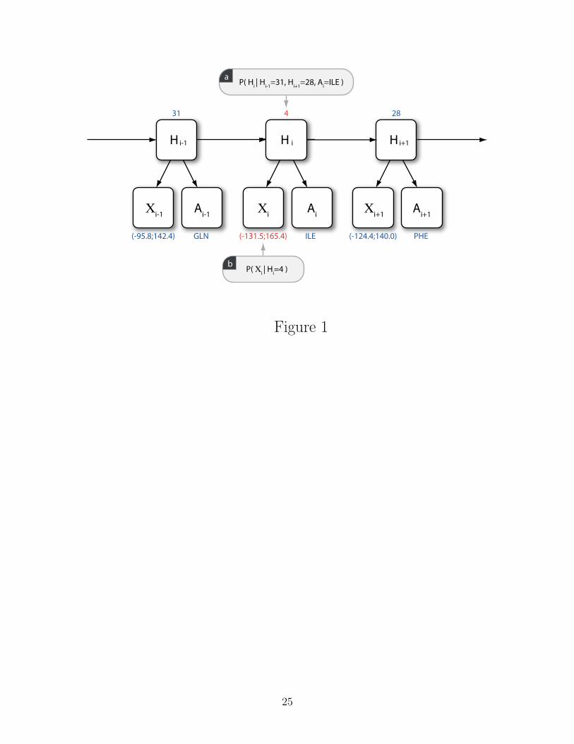
backbone-dbn, energy-basilisk, energy-compas). Figure 1 illustrates how dihedral angles

are sampled from a TORUSDBN-like model of the protein backbone. The practical details

on how probabilistic models can be incorporated in an energy function are discussed in the

Energy section below.

Efficient local updates

An important challenge in Monte Carlo simulations is to ensure efficient sampling in dense

states where proposed conformational changes will have a high probability of containing

self-collisions. In particular, pivot moves will typically have very poor acceptance rates in

this scenario. The solution is typically to expand the move set to include local moves, which

only change the atom positions within a small segment of the chain.

In addition to various established local move methods from the literature, PHAISTOS

includes a novel method, called CRISP4 (move-crisp), which is particularly well-suited for

5

this problem. Unlike other local move approaches7,8, CRISP is able to generate updates to

a segment of the chain without disrupting its local geometry. Often, local move algorithms

are designed as a two step process, where some angular degrees of freedom are modified

stochastically (pre-rotation), while other are modified deterministically to bring the chain

back to a closed state (post-rotation). From the work of Go and Scheraga16, it is known that

in general, six degrees of freedom are required for the post-rotation step. CRISP distinguishes

itself from previous methods by merging these two steps, modifying the stochastic pre-

rotation step so that it takes the resulting post-rotation step into account. More precisely, for

each application of the move, a random segment of the protein is selected, and a multivariate

Gaussian distribution is constructed over the angular change in the n−6 pre-rotation degrees

of freedom δχpre

P (δχpre) ∝ exp

(−1

2δχT

preλ(Cn−6 + STC6S)δχpre

). (1)

Here, C is an inverse diagonal covariance matrix specifying the desired fluctuations for

the individual angular degrees of freedom, S is a linear transformation mapping the pre-

rotational degrees of freedom to the corresponding post-rotational values, and λ is a scaling

parameter determining the size of the move. In effect, to first order, the method samples from

a distribution of closed chain structures, ensuring high quality local structure in all samples.

We have recently shown that this has a dramatic impact on simulation performance, in

particular for dense molecular systems4.

Low acceptance rates are also sometimes observed in side-chain moves. When using a fine-

grained force-field such as OPLS-AA/L, we have experienced that the standard resampling

of side-chains can be overly intrusive. Particularly in the case of side-chains involved in

several simultaneous hydrogen bonds, traditional moves tend to break all hydrogen bonds at

once, typically leading to the rejection of such updates. To avoid this problem, PHAISTOS

includes a novel move (sidechain-local) that, for a given side-chain, randomly selects an

atom that potentially participates in hydrogen bonds, and constrains its position using a

technique similar to that of the semi-local BGS backbone move4,9.

6

Energies

Two established force-fields are currently implemented within the framework: the PROFASI

force-field17, and the OPLS-AA/L18 force-field in combination with the GB/SA implicit

solvent model19. These represent two extremes in the range of force-fields available in the

literature: an ultrafast force-field modeling effective interactions in the presence of a solvent,

and a classic fine-grained molecular mechanics force-field combined with a more accurate

implicit solvent model. The two forcefields were selected to provide support for a broad range

of simulation tasks. The efficiency of the PROFASI forcefield makes it possible readily to

conduct reversible folding simulations of peptides and small proteins17. The OPLS forcefield

in combination with the GB/SA solvent model is more accurate, but also significantly slower,

and is typically used for exploring the details of native ensembles. It can also be used for

structure refinement, for instance of structures obtained in a reversible folding simulation

using PROFASI. For increased efficiency, all non-bonded force-field terms in both forcefields

have been implemented using the chaintree data structure20, which avoids recalculation of

energy contributions that are not modified in a given iteration of the simulation. Together

with effective local moves, this can result in a considerable computational speed-up.

PROFASI

The PROFASI force-field consists of four terms17

E = Eev + Ehb + Esc + Eloc (2)

where Eev captures excluded volume effects, Ehb is a hydrogen bond term, Esc is a side-chain

interaction term and Eloc concerns the local interactions along the chain. The excluded

volume potential is a simple r−12 interaction between all atom pairs, where r denotes the

distance between the atoms. The strength of a hydrogen bond in PROFASI depends on

the detailed geometry of the bond, parameterized through the N-H-O and H-O-C angles.

The side-chain potential consists of a charge-charge and a hydrophobicity contribution. For

each residue pair, these consist of a product between a conformation-dependent contact

strength and an energy that depends on the specific amino acid types involved in the bond.

7

Finally, the local energy term captures interactions between partial charges in neighbouring

peptide units along the chain, with a correction term for improved consistency with the

Ramachandran plot, and a side-chain torsion potential. Since bond angles and bond lengths

are assumed fixed during PROFASI simulations, no further local interactions are included.

A distinguishing feature of the PROFASI force-field is the presence of a global interaction

cutoff of 4.5A. While this necessarily excludes various long range interactions, it is also one

of the main reasons behind the efficiency of the force-field. Despite this restriction, the force-

field has been demonstrated to successfully fold a range of peptides and small proteins17,

while still being fast enough for many-body aggregation simulations21,22.

OPLS-AA/L

In contrast to PROFASI, the OPLS-AA/L force-field includes local terms for bond angles,

bond lengths and torsions. The bond angle and bond length potentials are simple harmonic

terms, while the torsion term has the form18

Etorsion =∑i

3∑j=1

wj(1 + (−1)j+1 cos(jθi)) (3)

where the outer sum iterates over all dihedrals θi. The non-bonded interactions include

standard Lennard-Jones and Coulomb potentials

Enb =∑i>j

wij

(4ϵij

((σijrij

)12

−(σijrij

)6)

+1

4πε0

qiqjrij

)(4)

where rij is the distance between atoms i and j, qi and qj are the corresponding partial

charges, ε0 is the vacuum permittivity and σij and ϵij are calculated using the combination

rules σij =√σiσj and ϵij =

√ϵiϵj. Finally, wij works to exclude interactions between atoms

that are separated by only a few covalent bonds. Thus, wij = 0.0 for direct neighbours (1,2)

and pairs separated by a single other atom (1,3), wij = 0.5 for pairs separated by two atoms

(1,4), and wij = 1.0 for all others.

Our implementation of OPLS-AA/L follows that of the Tinker simulation package23. We

ensured that energies produced by our program match those obtained when running Tinker.

8

GB/SA

The PROFASI force-field is parameterized to capture effective interactions in the presence of

a solvent. In contrast, OPLS should be combined with a suitable solvent model to reproduce

physiological conditions. In order to model the effect of the solvent on hydrophobic inter-

actions and electrostatics, we use the OPLS forcefield in combination with the Generalized

Born Surface Area (GB/SA) implicit solvent model19.

Many implicit solvent models express the solvation free energy Gsolv as a sum of non-polar

and electrostatic contributions

Gsolv = Gnpol +Gpol (5)

Here, Gnpol is the free energy of solvating the molecule with all the partial charges set to

zero, and Gpol is the reversible work required to increase the charges from zero to their full

values24. In GB/SA, the non-polar contribution Gnpol is assumed to be proportional to the

solvent accessible surface area, while the generalized Born approximation is used to calculate

the electrostatic solvation energy using the pairwise summation25

Gpol = − 1

8πε0

(1− 1

ε

) n∑i,j

qiqjfGB

(6)

where ε is the dielectric constant of the solvent and qi is the partial charge of atom i.

fGB =√r2ij + αiαj exp (−r2ij/4αiαj) is a function of the distance rij and of the so-called Born

radii α, which reflects the average distance of the charged atom to the dielectric medium. For

our implementation, the Born radii are calculated using an analytical expression proposed

by Still and coworkers19.

Incorporating Probabilistic Models in the Energy Function

When using moves that are based on probabilistic models such as TORUSDBN or BASILISK,

it gives rise to a bias in the simulation, which can be regarded as an implicit energy term.

In PHAISTOS, the energy contributions of these probabilistic models can also be evaluated

explicitly, by adding them as a term to the energy function. This makes it possible to use the

probabilistic models as energies in a simulation with a standard set of unbiased moves, or to

compensate for the bias of a move by adding the corresponding energy term with negative

9

weight. When used as energies, the values are reported in minus log-probabilities. In order

to facilitate the combination of classic energy terms with probabilistic terms, the energies

of physical force-fields such as PROFASI and OPLS-AA/L are likewise reported as minus

log-probabilities: they are multiplied by −1/kT , where T is the simulation temperature and

k is the Boltzmann constant.

As an example, for the TORUSDBN-like model in Figure 1, the log-likelihood for a given

state is

LL(X, A) = ln∑H

P (X, A, H) (7)

= ln∑H

P (X1|H1)P (A1|H1)P (H1)N∏i=2

P (Xi|Hi)P (Ai|Hi)P (Hi|Hi−1)

where X, A and H are the sequences of angle pairs, amino acid labels, and hidden node

labels, respectively, i is the residue index, and N is the sequence length. Each hidden node

label is the index of a component of the emission distributions of the model. For instance, the

Ramachandran distribution is modeled as a weighted sum of bivariate von Mises distribution

components14. The hidden nodes are “nuisance” parameters, and are therefore summed out

in the evaluation of the likelihood. Note that the sum runs over all possible hidden node

sequences, a calculation which can be done efficiently using dynamic programming14.

Observables

Observables in PHAISTOS allow a user to extract information about the current state of a

simulation. Examples of observables include root-mean-square-deviation (RMSD) (observable-

rmsd) and radius of gyration (observable-rg). In addition, all energy terms are also avail-

able as observables. A user can specify a selection of observables from the command line or

settings file, choosing how frequently they should be registered and in which format. While

most observables will return a single value, others have more elaborate outputs, such as

dumping of complete structural states to PDB files (observable-pdb) or to a molecular

trajectory file in the Gromacs XTC format (observable-xtc-trajectory)26. Finally, ob-

servables can be dumped to the header or as b-factors in outputted PDB-files. The latter

10

makes it possible to annotate structures with residue-specific information, such as the num-

ber of contacts, degree of burial, or more sophisticated evaluations of the environment of

each residue27.

Monte Carlo

Although PHAISTOS can be used for Monte Carlo minimization, the primary focus of the

framework is Markov chain Monte Carlo simulation, where the goal is to produce samples

from the Boltzmann distribution corresponding to a given force-field at a specified temper-

ature. All moves in PHAISTOS are therefore designed to be compatible with the property

of detailed balance, in the sense that their proposal probabilities can be evaluated. That is,

for a move from state x to state x′

π(x)P (x→ x′) = π(x′)P (x′ → x) (8)

where π(x) is the stationary distribution, and P (x → x′) is the probability of moving from

state x to x′ using a given move. Factoring P (x→ x′) into a selection probability Ps and an

acceptance probability Pα, we have

Pα(x→ x′)

Pα(x′ → x)=π(x′)Ps(x

′ → x)

π(x)Ps(x→ x′)(9)

Most of the moves are symmetric, in the sense that Ps(x′ → x)/Ps(x → x′) = 1. However,

for moves such as the local and semi-local moves, this is not the case, and it is important that

this bias be correctly compensated for. Implementation-wise, each Move object is responsible

for calculating the bias that it introduces, and the Monte Carlo class will then compensate

for it when necessary.

Metropolis-Hastings

The most common way to ensure that eq. (9) is fulfilled is to use the Metropolis-Hastings

(MH) acceptance criterion

Pα(x→ x′) = min

(1,π(x′)Ps(x

′ → x)

π(x)Ps(x→ x′)

)(10)

11

This is the default simulation method used in PHAISTOS (monte-carlo-metropolis-hastings).

It is useful for exploring near-native ensembles, and can be efficient when simulating at the

critical temperature of a system. However, for more complicated systems, MH simulations

tend to spend excessive periods of time exploring local minima, leading to poor mixing and

therefore slow convergence.

Generalized Ensembles

To avoid the mixing problems associated with standard Metropolis-Hastings simulations,

PHAISTOS includes support for conducting simulations in generalized ensembles28. Rather

than sampling directly from the Boltzmann distribution, the central idea is to generate

samples from a modified distribution, and subsequently reweight the obtained statistics to

the Boltzmann distribution at a desired temperature. The acceptance criterion becomes

Pα(x→ x′) = min

(1,w(x′)Ps(x

′ → x)

w(x)Ps(x→ x′)

)(11)

for a given weight function w(x). The typical choice is the multi-canonical ensemble29,

corresponding to a flat distribution over energies. That is, w(x) = 1/g(E(x)), where E(x) is

the energy associated with conformational state x, and g is the number of states associated

with a given energy (density of states). Another example is the 1/k ensemble, which attempts

to provide ergodic sampling while maintaining primary focus on the low energy states30. In

this case, the weight function is w(x) = 1/k(E(x)), where k(E(x)) =∫ E(x)

−∞ g(E)dE. It can

be shown that this is approximately equivalent to a flat histogram over ln(E(x))30.

We have recently developed an automated method, MUNINN, for estimating the weights

w in generalized ensemble simulations (http://muninn.sourceforge.net/). It employs

the generalized multi-histogram equations31, and uses a non-uniform adaptive binning of

the energy space, ensuring efficient scaling to large systems. In addition, MUNINN allows

weights to be restricted to cover a limited temperature range of interest. The MUNINN

functionality is seamlessly integrated into PHAISTOS, and can be activated by selecting the

corresponding Monte Carlo engine (monte-carlo-muninn).

12

Monte Carlo Minimization

PHAISTOS contains a few simulation algorithms that are directed at optimization, rather

than sampling. These include a simulated annealing class (monte-carlo-simulated-annealing)

and a greedy Monte Carlo optimization class (monte-carlo-greedy-optimization), which

are useful in cases where the user is interested in a single low-energy structure, rather than

a full structural ensemble.

Program Design

The framework is designed to be modular, both in software design and in the choices exposed

to the user from the command line or settings file. As illustrated in the UML diagram in

Figure 2, all energy terms are derived from the same base class, and implement the same

interface. Energy functions can easily be constructed from the command line or settings file

by including the energy terms of interest. Moves and Monte Carlo simulation algorithms are

structured in a similar way. This design makes it straightforward to implement new energy

terms, moves or simulation algorithms with little knowledge of the overall code. Iterators

are provided for easy iteration over atoms or residues in a molecule. In addition, caching

and rapid determination of interacting atom pairs is made possible by an implementation of

the chaintree algorithm20.

Finally, through a modular build-system, developers can readily write their own modules

utilizing the library. Modules are separate code entities that are auto-detected by the build

system when present, and can be enabled and disabled at compile time, making it easy to

share code among collaborators.

Example

We include a step-by-step walk-through of the PHAISTOS simulation process. The goal is

to conduct a reversible folding simulation of the 20-residue beta3s peptide32, demonstrating

several of the features described above.

The user interface of PHAISTOS is designed to make it as easy as possible to set up

13

simulations. Almost all options have default values, and it is therefore usually sufficient to

supply only a few input options to the program. The program behavior can then gradually

be fine-tuned using additional options in the configuration file later on. For this particular

example, we use the following command from the command line

$ ./phaistos --aa-file beta3s.aa \

--energy profasi-cached backbone-dbn[weight:-1] \

--move backbone-dbn sidechain-uniform semilocal-dbn-eh \

--threads 8 --temperature 283 \

--monte-carlo muninn[min-beta:0.6,max-beta:1.1] \

--observable backbone-dbn rmsd[reference-pdb-file:beta3s.pdb] \

--observable xtc-trajectory

The aa-file argument specifies that we are reading an amino acid sequence from a file. The

energy and move options select the relevant energy terms and moves, respectively. In this

case, we use a cached version of the PROFASI force-field, and sample using TORUSDBN

moves, uniformly distributed side-chain moves and BGS moves using the TORUSDBN as

a prior. We specify that the simulation should be conducted in 8 parallel threads and

set the temperature to 283K. MUNINN is chosen to be the Monte Carlo engine, using a β

(inverse temperature) range of [0.6; 1.1]. These β factors are unit-less, specified relative to the

inverse temperature, and thus correspond to a temperature range of [(1.1 · 1/283K)−1; (0.6 ·

1/283K)−1] = [257K; 472K]. Finally, we specify that we wish to record observables about

the backbone-dbn energy, the RMSD to the native state, and dump structures to an XTC

trajectory file. Apart from the RMSD observable, we do not provide the program with any

information about the structure of the protein, and the simulation will therefore start in a

random extended state.

To illustrate the framework’s support for various types of biased sampling, this example

uses a variant where the TORUSDBN bias is included in the sampling, and explicitly sub-

tracted in the energy (i.e. the weight:-1 option of backbone-dbn). This means that the bias

cancels out when extracting statistics at β = 1, thus producing unbiased estimates at 283K.

The simulation will produce a flat histogram over the expected energy range corresponding

14

to the specified temperature range ([< E >257K ;< E >472K ]).

We ran PHAISTOS with the settings above on an eight-core 3.4GHz Intel Xeon pro-

cessor for one week. Figure 3 gives an overview of the results. The free energy plot in

Figure 3(a) shows the distribution of energy versus RMSD extracted directly from the sam-

ples dumped during the simulation. Since the samples were generated using a generalized

ensemble technique, they must be reweighted to retrieve the statistics according to the Boltz-

mann distribution at the specified temperature. This is done using a script included in the

MUNINN module, resulting in the plot in Figure 3(b).

To find representative structures in the ensemble, we use the PLEIADES clustering mod-

ule33, included in the framework. Again, it is important to remember that the raw data are

produced in a generalize ensemble setting and must be reweighted. We ran the RMSD-based

weighted k-means method implemented in the PLEIADES module to select the highlighted

structures in Figure 3.

From the analysis above, we conclude that at 283K, the protein is marginally stable in

the PROFASI force-field, with native-like populations at 2A and 4A RMSD, but also a signif-

icant population of unstructured or helical conformations. These results are in approximate

agreement with experiments, which suggest a folded population of between 13% and 31%32.

This result is compatible with a previously published simulation of the same protein using

an unbiased simulation technique17.

RESULTS

To illustrate the versatility of PHAISTOS, we highlight several recently published applica-

tions of the framework.

Structure prediction and inference

An example of the applicability of PHAISTOS in the context of protein structure prediction

is found in a recent study on potentials of mean force34. The study demonstrates how

probabilistic models of local protein structure such as TORUSDBN and BASILISK can

be combined with probabilistic models of nonlocal features, such as hydrogen bonding or

15

compactness, using a simple probabilistic technique.

The framework has also been applied for inference of protein structure from Small-angle

X-ray scattering (SAXS) and Nuclear Magnetic Resonance (NMR) experimental data. SAXS

data contains low resolution information on the overall shape of a protein, which can be useful

for determining the relative domain positions and orientations in multi-domain proteins or

complexes. This can for instance be used to infer structural models of multi-domain proteins

connected by flexible linkers, given the atomic structures of the individual domains. Such

calculations require efficient back-calculation of SAXS curves, which is made possible through

a coarse grained Debye method35,36.

NMR experimental data can provide high resolution structural information which can

improve the accuracy of a simulation. PHAISTOS contains preliminary support for sam-

pling conditional on chemical shift data, which is known to contain substantial information

on the local structure of a protein37,38. Furthermore, the framework was recently used for in-

ferential structure determination using pair-wise distances obtained from NOE experiments,

with TORUSDBN and BASILISK as prior distribution for the protein’s backbone and side

chains39.

Efficient clustering

Efficiently clustering a large number of protein structures is an important task in protein

structure prediction and analysis. Typically, clustering programs require costly RMSD cal-

culations for many pairs in the set of structures. PHAISTOS contains a clustering module

called PLEIADES that uses a k-means clustering approach40 to reduce the number of pair-

wise RMSD distance calculations. Furthermore, PLEIADES includes support for replacing

the RMSD distance computations with distances between vectors of Gauss integrals41, which

provides dramatic computational speedups33.

Native ensembles

The energy landscape around the native state tends to be rugged, making it challenging to

sample such states efficiently1. For these tasks, the CRISP backbone move is particularly well

16

suited, given its ability to propose subtle, non-disruptive updates to the protein backbone.

Monte Carlo simulations using this move were recently shown to explore conformational

space with an efficiency on par with molecular dynamics, outperforming the current state-

of-the-art in local Monte Carlo move methods4.

The TYPHON module42 rapidly explores near-native ensembles by using the CRISP

move in combination with a user-defined set of non-local restraints. Local structure is

under the control of probabilistic models of the backbone (TORUSDBN) and side chains

(BASILISK), while non-local interactions such as hydrogen bonds and disulfide bridges are

heuristically imposed as Gaussian restraints. TYPHON can be seen as a “null model” of con-

formational fluctuations in proteins: it rapidly explores the conformational space accessible

to a protein given a set of specified restraints.

DISCUSSION

The relevance of a new software package should be assessed relative to already existing

packages in the literature. We acknowledge that in our case, there are a number of such

alternatives already available. We describe the most important ones here, focusing on the

differences to the framework presented in this paper.

Of the available Monte Carlo software packages, the ROSETTA package11 is perhaps

the most widely used, and has an impressive track record for protein structure prediction

and design43. The package focuses primarily on structure/sequence prediction (optimiza-

tion) rather than simulation, and consequently, many of the moves in ROSETTA are not

compatible with the property of detailed balance.

PHAISTOS also has some overlap with the PROFASI simulation package44, in the sense

that both implement the BGS move9 and the PROFASI energy function17. The PROFASI

simulation program was designed as a tool for studying protein aggregation, and is thus

highly optimized for many-chain simulation using their lightweight forcefield and under the

assumption of fixed bond angles. PHAISTOS aims to provide a greater flexibility in the

choice of energies and a wider selection of moves, and is not limited to a fixed bond-angle

representation.

17

The closest alternatives to PHAISTOS are perhaps the CAMPARI software package1 and

the Monte Carlo package in CHARMM2, which both provide functionality for conducting

Markov chain Monte Carlo simulations using various force-fields and moves. Compared with

PHAISTOS, the selection of force-fields and moves differ, and the focus is different. For

instance, PHAISTOS has a strong focus on sampling using probabilistic models of local

structure, which is not supported by either of the two alternatives.

The current version of the PHAISTOS framework has several limitations. To a user

familiar with molecular dynamics software, the primary limitation will presumably be the

lack of explicit solvent models in the framework. The large conformational moves that pro-

vide the sampling advantage of Monte Carlo simulations are difficult to combine with an

explicit solvent representation. In line with other Monte Carlo simulation packages, PHAIS-

TOS is therefore currently limited to implicit solvent simulations. Another limitation is that

PHAISTOS can currently only simulate a single polypeptide at a time. This restriction will

be removed in the next release of the software, which will also include implementations of

several new force-fields.

As the list of applications demonstrates, even in its current form, the framework provides

the necessary tools for conducting relevant MCMC simulations of protein systems. The

framework incorporates generalized ensembles and novel Monte Carlo moves, including moves

that incorporate structural priors as proposal distributions. These features are unique to this

framework, and have been shown to increase sampling efficiency considerably.

The software is freely available under the GNU General Public License v3.0. All source

code is fully documented using the Doxygen system (http://www.doxygen.org) and a user

manual is available for detailed descriptions on how to set up simulations. Both sources of

information are accessible via the PHAISTOS web site, http://phaistos.sourceforge.

net.

ACKNOWLEDGMENTS

This work was supported by the Danish Council for Independent Research [FNU272-08-0315

to W.B., FTP274-06-0380 to K.S, FTP09-066546 to S.O., J.V., FTP274-08-0124 to K.E.J.],

the Danish Council for Strategic Research [NABIIT2106-06-0009 to J.F., Ti.H., C.A., M.B.],

18

the Novo Nordisk STAR Program [A.S.C.], a Hallas-Møller stipend from the Novo Nordisk

Foundation [K.L.L.] and Radiometer (DTU) [S.B.].

19

References

1. A. Vitalis and R.V. Pappu, Annu. Rep. Comput. Chem. 2009, 5, 49–76.

2. J. Hu, A. Ma and A.R. Dinner, J. Comput. Chem. 2006, 27, 203–216.

3. J.P. Ulmschneider, M.B. Ulmschneider and A. Di Nola, J. Phys. Chem. B. 2006, 110,

16733–16742.

4. S. Bottaro, W. Boomsma, K. E. Johansson, C. Andreetta, T. Hamelryck and

J. Ferkinghoff-Borg, J. Chem. Theory Comput. 2012, 8, 695–702.

5. M. Habeck, M. Nilges and W. Rieping, Phys. Rev. Lett. 2005, 94, 18105.

6. M. R. Betancourt, J. Chem. Phys. 2005, 123, 174905–174907.

7. C. Smith and T. Kortemme, J. Mol. Biol. 2008, 380, 742–756.

8. J. P. Ulmschneider and W. L. Jorgensen, J. Chem. Phys. 2003, 118, 4261–4271.

9. G. Favrin, A. Irback and F. Sjunnesson, J. Chem. Phys. 2001, 114, 8154–8158.

10. R. L. Dunbrack and F. E. Cohen, Protein Sci. 1997, 6, 1661–1681.

11. A. Leaver-Fay, M. Tyka, S.M. Lewis, O.F. Lange, J. Thompson, R. Jacak, K. Kaufman,

P.D. Renfrew, C.A. Smith, W. Sheffler et al., Methods Enzymol. 2011, 487, 545–574.

12. T. Przytycka, Proteins. 2004, 57(2), 338–344.

13. T. Hamelryck, J.T. Kent and A. Krogh, Plos. Comput. Biol. 2006, 2, e131.

14. W. Boomsma, K.V. Mardia, C.C. Taylor, J. Ferkinghoff-Borg, A. Krogh and T. Hamel-

ryck, Proc. Natl. Acad. Sci. U. S. A. 2008, 105, 8932.

15. T. Harder, W. Boomsma, M. Paluszewski, J. Frellsen, K.E. Johansson and T. Hamelryck,

BMC Bioinformatics. 2010, 11, 306.

16. N. Go and H.A. Scheraga, Macromolecules. 1970, 3(2), 178–187.

20

17. A. Irback, S. Mitternacht and S. Mohanty, PMC Biophysics. 2009, 2, 2.

18. G.A. Kaminski, R.A. Friesner, J. Tirado-Rives and W.L. Jorgensen, J. Phys. Chem. B.

2001, 105, 6474–6487.

19. D. Qiu, Shenkin P.S., F.P. Hollinger and W.C. Still, J. Phys. Chem. A. 1997, 101,

3005–3014.

20. I. Lotan, F. Schwarzer, D. Halperin and J.C. Latombe, J. Comput. Biol. 2004, 11,

902–932.

21. A. Irback and S. Mitternacht, Proteins. 2007, 71(1), 207–214.

22. D.W. Li, S. Mohanty, A. Irback and S. Huo, PLoS Comput. Biol. 2008, 4(12), e1000238.

23. J.W. Ponder and F.M. Richards, J. Am. Chem. Soc. 1987, 8(7), 1016–1024.

24. B. Roux and T. Simonson, Biophys. Chem. 1999, 78(1), 1–20.

25. W.C. Still, A. Tempczyk, R.C. Hawley and T. Hendrickson, J. Am. Chem. Soc. 1990,

112(16), 6127–6129.

26. B. Hess, C. Kutzner, D. van der Spoel and E. Lindahl, J. Chem. Theory Comput. 2008,

4(3), 435–447.

27. K.E. Johansson and T. Hamelryck, Proteins (In press). 2013.

28. U.H.E. Hansmann and Y. Okamoto, J Comput. Chem. 1997, 18, 920–933.

29. B.A. Berg and T. Neuhaus, Phys. Rev. Lett. 1992, 68(1), 9.

30. B. Hesselbo and RB Stinchcombe, Phys. Rev. lett. 1995, 74(12), 2151–2155.

31. J. Ferkinghoff-Borg, J. Eur. Phys. J. B. 2002, 29, 481–484.

32. E. De Alba, J. Santoro, M. Rico and M. Jimenez, Protein Sci. 1999, 8, 854–865.

33. T. Harder, M. Borg, W. Boomsma, P. Røgen and T. Hamelryck, Bioinformatics. 2012,

28, 510–515.

21

34. T. Hamelryck, M. Borg, M. Paluszewski, J. Paulsen, J. Frellsen, C. Andreetta,

W. Boomsma, S. Bottaro and J. Ferkinghoff-Borg, PLoS ONE. 2010, 5, e13714.

35. K. Stovgaard, C. Andreetta, J. Ferkinghoff-Borg and T. Hamelryck, BMC Bioinformat-

ics. 2010, 11, 429.

36. N.G. Sgourakis, O.F. Lange, F. DiMaio, I. Andre, N.C. Fitzkee, P. Rossi, G.T. Monte-

lione, A. Bax and D. Baker, J. Am. Chem. Soc. 2011, 133(16), 6288–6298.

37. A. Cavalli, X. Salvatella, C.M. Dobson and M. Vendruscolo, Proc. Natl. Acad. Sci. U.

S. A. 2007, 104, 9615.

38. Y. Shen, O. Lange, F. Delaglio, P. Rossi, J.M. Aramini, G. Liu, A. Eletsky, Y. Wu, K.K.

Singarapu, A. Lemak et al., Proc. Natl. Acad. Sci. U. S. A. 2008, 105, 4685.

39. S. Olsson, W. Boomsma, J. Frellsen, S. Bottaro, T. Harder, J. Ferkinghoff-Borg and

T. Hamelryck, J. Magn. Reson. 2011, 213, 182–186.

40. S. Lloyd, IEEE Trans. Inf. Theory. 1982, 28, 129–137.

41. P. Røgen and B. Fain, Proc. Natl. Acad. Sci. U. S. A. 2003, 100, 119.

42. T. Harder, M. Borg, S. Bottaro, W. Boomsma, S. Olsson, J. Ferkinghoff-Borg and

T. Hamelryck, Structure. 2012, 20, 1028 – 1039.

43. R. Das and D. Baker, Annu. Rev. Biochem. 2008, 77, 363–382.

44. A. Irback and S. Mohanty, J. Comput. Chem. 2006, 27(13), 1548–1555.

45. Schrodinger, LLC. The PyMOL Molecular Graphics System, Version 0.99rc6.

22

Figure 1: An illustration of a simplified version of the TORUSDBN model of backbone

local structure, showing the architecture of the dynamic Bayesian network (DBN), and an

example of values for the individual nodes. Each A node is a discrete distribution over amino

acids, while each X node is a bivariate distribution over (ϕ, ψ) angle pairs. The hidden node

(H) sequence is a Markov chain of discrete states, representing the sequence of residues

in a protein chain. Each hidden node state corresponds to a particular distribution over

angle pairs and amino acid labels. The values highlighted in red are the result of a single

resampling step of the (ϕ, ψ) angle pair at some position i in the chain: a) The hidden node

state Hi is resampled based on the current values of the values of neighbouring H values and

the amino acid label at position i (P (Hi|Hi−1, Hi+1, Ai) ∝ P (Hi|Hi−1)P (Hi+1|Hi)P (A|Hi));

b) A (ϕ, ψ) value is drawn from the bivariate angular distribution corresponding to the

sampled H value (P (Xi|Hi)). A full description of the TORUSDBN model can be found in

the original publication14.

Figure 2: A UML-diagram of the major classes in the PHAISTOS library (black diamond:

composition, white diamond: aggregation, arrow: inheritance). A MonteCarlo simulation

object contains a MoveCollection object, which consists of a selection of moves, and an En-

ergy object, which is comprised of a number of energy terms (TermOpls* and TermProfasi*

denote the entire set of OPLS and PROFASI energy terms, respectively). Note that the

probabilistic models (BackboneDBN/BasiliskDBN/CompasDBN) are available both as en-

ergy terms and as moves. A detailed description of all classes can be found in the Doxygen

documentation on the PHAISTOS web site.

23

Figure 3: Illustration of a reversible folding simulation of the beta3s peptide in PHAIS-

TOS. The simulation was conducted with the PROFASI force-field, using the MUNINN

multihistogram method and a set of moves including TORUSDBN as a dihedral proposal

distribution. The bias introduced by TORUSDBN is compensated for to ensure correctly

distributed samples. a) Free energy plot as a function of energy and RMSD in the multi-

canonical (flat histogram) ensemble. b) Free energy plot as a function of energy and RMSD,

reweighted to the canonical ensemble at 283K. c-f) Representative cluster medoids found

with reweighted clustering using the PLEIADES module, compared to the native struc-

ture32 (shown in black). Figures created using Pymol45. g) RMSD vs time of one of the

eight threads in the simulation.

24

H i H i+1H i-1

Ai

Χi

Ai-1

Χi-1

Ai+1

Χi+1

GLN

31 4 28

(-95.8;142.4) (-131.5;165.4) (-124.4;140.0)ILE PHE

a

b

P( Hi | H

i-1=31, H

i+1=28, A

i=ILE )

P( Χi | H

i=4 )

Figure 1

25

Energy

EnergyTerm

TermRmsd TermRg

TermBackboneDBN

TermClashFast

MonteCarlo

TermProfasiEV2TermProfasiHB2TermProfasiH2TermProfasiL2TermProfasiLS2TermProfasiSC2TTTTTTTTerermProfasiSC2TermProfasi*TermGbsa TermOplsAB2TermOplsBS2TermOplsC2TermOplsI2TermOplsT2TTTTTTTerermOplsT2TermOpls*

MoveCollection

MonteCarloMetropolisHastings MonteCarloSimulatedAnnealing

Simulation Opt imizat ion

Move

MoveCrankshaft

MoveBackboneDBN

MovePivotLocalMovePivotUniform

MoveSidechainLocal

MoveSidechainUniform

MoveCRA

MoveCRISPMoveBGS

MonteCarloMuninn

MoveSidechainRotamer TermSaxsDebye

TermConstrainDistancesMoveSidechainDBN

BackboneDBN FB5DBNTorusDBN BasiliskDBN/CompasDBN

TermSidechainDBN

MonteCarloGreedyOptimization

Figure 2

26

b

ad e

c

g

f

5

0 1 2 3 4 5 6

10

15

Monte Carlo steps (108)

RMSD

(Å)

●● ●

●

20

40

60

804

-ln(P(E))

6

8

>10

0 2 4 6 8 10 12 14 16 18

E (k

cal/

mo

l)

RMSD (Å)

20

40

60

80

0

4-ln(P(E))

6

8

>10

2 4 6 8 10 12 14 16 18

E (k

cal/

mo

l)

RMSD (Å)

reweighting

●●●

(kca

l/m

ol)

(kca

l/m

ol)

(kca

l/m

ol)

(kca

l/m

ol)

(kca

l/m

ol)

(kca

l/m

ol)

(kca

l/m

ol)

(kca

l/m

ol)

(kca

l/m

ol)

(kca

l/m

ol)

(kca

l/m

ol)

(kca

l/m

ol)

(kca

l/m

ol)

(kca

l/m

ol)

(kca

l/m

ol)

(kca

l/m

ol)

(kca

l/m

ol)

(kca

l/m

ol)

(kca

l/m

ol)

(kca

l/m

ol)

(kca

l/m

ol)

(kca

l/m

ol)

(kca

l/m

ol)

(kca

l/m

ol)

(kca

l/m

ol)

(kca

l/m

ol)

(kca

l/m

ol)

(kca

l/m

ol)

(kca

l/m

ol)

(kca

l/m

ol)

(kca

l/m

ol)

(kca

l/m

ol)

(kca

l/m

ol)

(kca

l/m

ol)

(kca

l/m

ol)

(kca

l/m

ol)

(kca

l/m

ol)

(kca

l/m

ol)

(kca

l/m

ol)

(kca

l/m

ol)

(kca

l/m

ol)

(kca

l/m

ol)

(kca

l/m

ol)

(kca

l/m

ol)

(kca

l/m

ol)

(kca

l/m

ol)

(kca

l/m

ol)

(kca

l/m

ol)

(kca

l/m

ol)

(kca

l/m

ol)

(kca

l/m

ol)

(kca

l/m

ol)

(kca

l/m

ol)

(kca

l/m

ol)

(kca

l/m

ol)

(kca

l/m

ol)

(kca

l/m

ol)

(kca

l/m

ol)

(kca

l/m

ol)

(kca

l/m

ol)

(kca

l/m

ol)

(kca

l/m

ol)

(kca

l/m

ol)

(kca

l/m

ol)

(kca

l/m

ol)

●●

888888888888888888888888●●●

Figure 3

27