pH Emission Spectrum Emission(3 λ) λ1 λ2 λ3 A λ λ1λ2λ3λ1λ2λ3 A Ex 1 Emission(3 λ) λ1λ2λ3λ1λ2λ3 A Ex 2 Emission(3 λ) λ1λ2λ3λ1λ2λ3 A Ex 3 λ1λ2λ3λ1λ2λ3.

By : S. M. Sajjadi

Supervisor : Dr. H. Abdollahi

June 2011

pH Emission Spectrum

Emission(3λ)

λ1 λ2 λ3

A

λ

λ1

λ2

λ3

A

Ex1

Emission(3λ)λ1

λ2

λ3

A

Ex2

Emission(3λ)

λ1

λ2

λ3

A

Ex3

λ1

λ2

λ3

Second order

(matrix)

Ex1 Ex2 Ex3

Second order data

λ1 λ2 λ3

A

λ

A

1

λ1

λ2

λ3Ex1 Ex2 Ex3

pH

Exλ

pH

Emission(3λ)λ1

λ2

λ3Ex1

Emission(3λ)

λ1

λ2

λ3Ex2

Emission(3λ)λ1

λ2

λ3Ex3

pH

pH

pH

Ex1 Ex2 Ex3

Ex1 Ex2 Ex3

Ex1 Ex2 Ex3

3-way Methods: PARAFAC, …

2

λem.

λex

M

pH λex

λem.

pH

Second-order, i.e., matrix data for a given sample can be

produced in a variety of ways:

one of them is Fluorescence spectroscopy

3

M

Sample

pH

Sample

pH

λ

λ

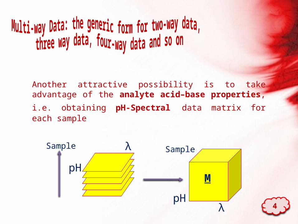
Another attractive possibility is to take advantage of the analyte acid–base properties, i.e. obtaining pH-

Spectral data matrix for each sample

4

Soft modeling parallel factor analysis method attempts to

decompose a three-way data into the product of three

significantly smaller matrices.

EzyxD vecvecP

pppp

1

K

I

= +

B

ID

KC K

I

E

JA

PPP

Parallel Factor Analysis

5

The popularity of PARAFAC model in resolving multi-way data is due to its unique properties

The reason for the importance of uniqueness of solutions is clear: obtaining unique solutions allows for an unambiguous interpretation of the estimated parameters (spectra, chromatograms, etc.) in terms of the chemical system. In short, uniqueness generates fundamental insight into the chemistry of the studied system.

6

oIn some of three-way data array, some factors are strictly proportional in one mode of a three-way array and the PARAFAC may lead to false minima.

oHowever, appropriate selection of the initial parameters and restrictions (e.g. non-negativity) still make PARAFAC useful in this regard .

7

o The non-negativity, unimodality and orthogonality constraints are optional selection in the PARAFAC rutine belonging to N-way toolbox

o There are not any reports on the applying hard modeling on some species to reduce rotational ambiguity in the PARAFAC solution.

8

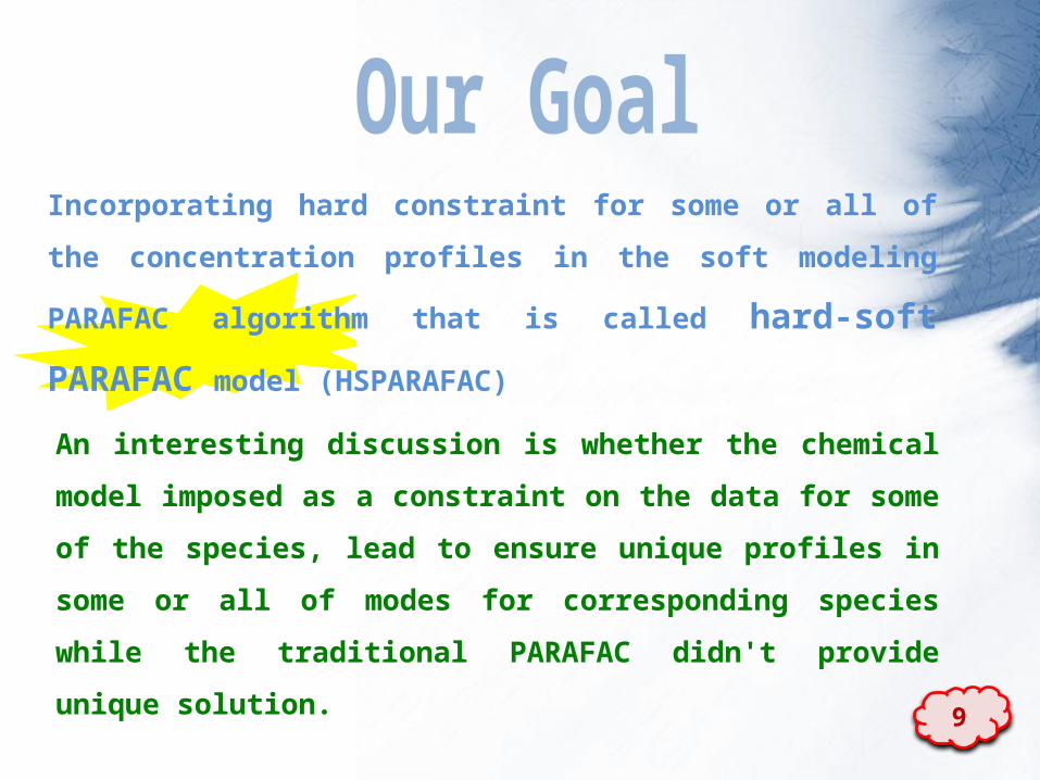
Incorporating hard constraint for some or all of the

concentration profiles in the soft modeling PARAFAC

algorithm that is called hard-soft PARAFAC model

(HSPARAFAC)

An interesting discussion is whether the chemical

model imposed as a constraint on the data for some

of the species, lead to ensure unique profiles in some

or all of modes for corresponding species while the

traditional PARAFAC didn't provide unique solution. 9

Alternating least squares PARAFAC algorithm

Algorithms for fitting the PARAFAC model are usually

based on alternating least squares. This is

advantageous because the algorithm is simple to

implement, simple to incorporate constraints in, and

because it guarantees convergence. However, it is

also sometimes slow.10

The PARAFAC algorithm begins with an initial guess of

the two loading modes

The solution to the PARAFAC model can be found by

alternating least squares (ALS) by successively assuming the

loadings in two modes known and then estimating the

unknown set of parameters of the last mode.

Determining the rank of three-way array

11

Step1. Determining of A profile

Suppose initial estimates of B and C loading modes are given

=

K

J

I

Matricizing

I

JK

IJK

N

N

A = XZA+

12

X (I×J×K) X (J×IK)

B =X ZB+

=

J

IKN

J

IK N

Matricizing

X(J×IK) = B(J×N)(CA)T = B ZBT

13

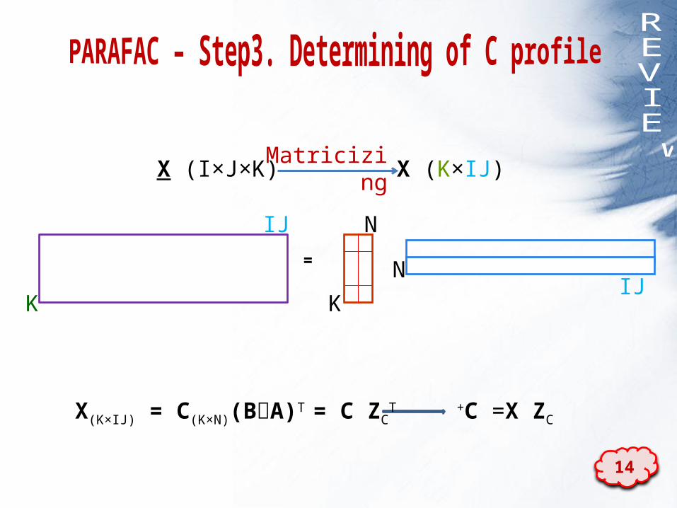
X (I×J×K) X (K×IJ)

=

KIJ

N

K

IJ N

Matricizing

C =X ZC+X(K×IJ) = C(K×N)(BA)T = C ZC

T

14

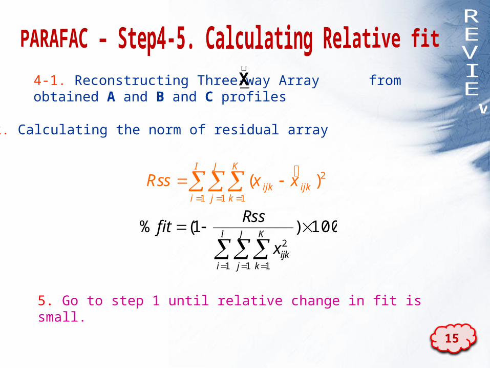
5. Go to step 1 until relative change in fit is small.

4-1. Reconstructing Three-way Array from obtained A and B and C profiles

4-2. Calculating the norm of residual array

2

1 1 1

( )I J K

ijk ijki j k

Rss x x

X

100)1(%

1 1 1

2

I

i

J

j

K

kijkx

Rssfit

15

Initialize B and C

2 A = X(I×JK ) ZA(ZAZA)−1

3 B = X(J×IK ) ZB(ZBZB)−1

4 C = X(K×JI ) ZC(ZCZC)−1

Given: X of size I × J × K

Go to step 1 until relative change in fit is small

1

5

ZA=CB

ZB=CA

ZC=BA

16

17

Chemical Model

HA A- +H+

K

I

= +B

ID

K C K

IE

JA

Hard constraint for two components

Nonlinear fitting constraint

AA

AALSAFIT

18

Initialize B and C

2 A = X(I×JK ) ZA(ZAZA)−1

3 B = X(J×IK ) ZB(ZBZB)−1

4 C = X(K×JI ) ZC(ZCZC)−1

Given: X of size I × J × K

Go to step 1 until relative change in fit is small

1

5

ZA=CB

ZB=CA

ZC=BA

Hard Constraint 2-1

19

20

HA A- + H+

λem.

λex

M

pH λex

λem.

pH

21

22

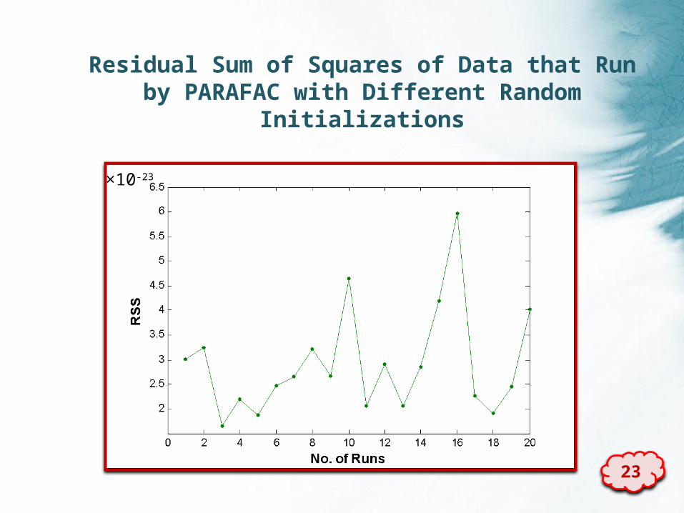
×10-23

Residual Sum of Squares of Data that Run by PARAFAC with Different Random

Initializations

23

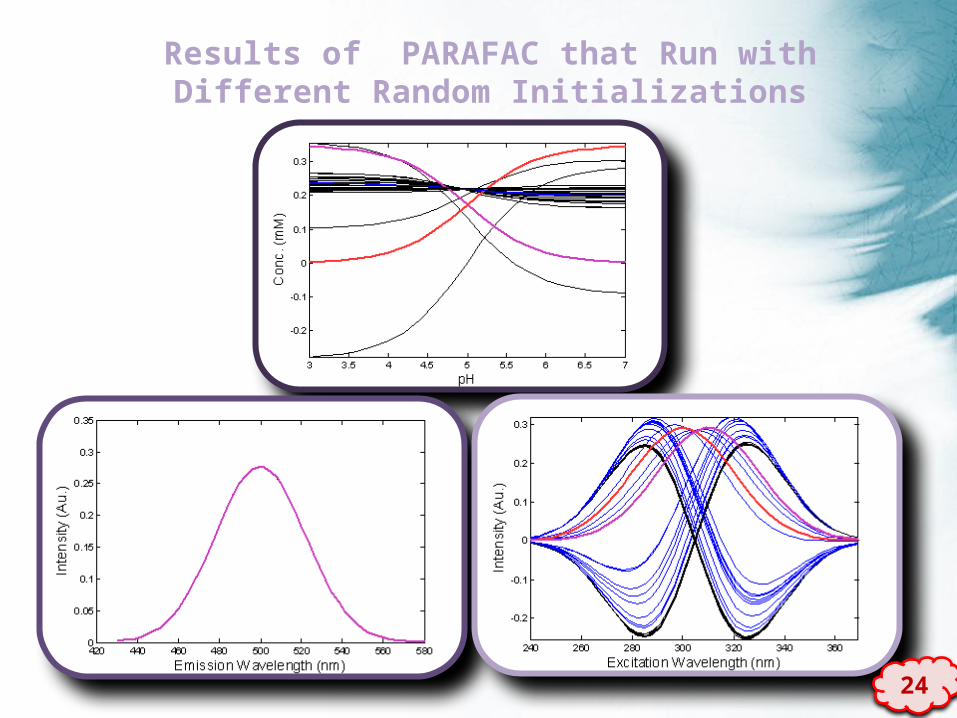
Results of PARAFAC that Run with Different Random Initializations

24

pKa =5

25

HPARAFAC PARAFACData Case

IpKa Time No. of iter.

Time No. of iter.

5.00 0.33 13 0.02 2 Noise free

5.00 0.25 12 0.023 4 Noisy

26

HA A- + H+

HB B- + H+

Closure Rank Deficiency

λem.

λex

M

pH λex

λem.

pH

27

Ct1 = a Ct2[HA] + [A-] = a([HB] + [B-])

[HB] + [B-] = Ct2

[HB] = Ct2 [H+]

[H+] + Ka2

C K[B-] = t2 a2

[H+] + Ka2

HB B- + H+

[HA] = Ct1 [H+]

[H+] + Ka1

C K[A-] = t1 a1

[H+] + Ka1

HA A- + H+

[HA] + [A-] = Ct1

28

Case IV

emHA = emHBCase III b

emHA = emA-Case III a

B- is not spectroscopic active# emHA = emHBCase II.b

B- is not spectroscopic active, emHA

= emA-Case II.a

Description of Three-way Data

emHA = emA-

emHA = emHB

Closure Rank Deficiency

Five Different Simulation Three-way Data

HA A- +H+

HB B- +H+

HA A- +H+

HB B- +H+

HA A- +H+

HB B- +H+

HA A- +H+

HB B- +H+

HA A- +H+

HB B- +H+

29

Results of PARAFAC and HSPARAFAC for Case IIa Three-way Data

HA A- +H+

HB B- +H+

B- is not Spectroscopic active

emHA=emA-

Hard constraints has been applied on rank overlap components

Unique Time(s)Iter. Iter.Methods

Free Noise Data Noisy Data

5.00

839 7.47

552 4.94

170

87

2.57

1.41

Time(s) pKapKa

5.00

Rank overlap problem

.PARAFAC

HSPARAFAC

30

The unique Span spanned by excitation and pH profiles of rank overlapped species

HA and A-

11 12

21 22

t t=

t t

T 12

21

1 t=

t 1

T

1t

t1

tt1

1

21

12

2112

1T

ex

pH=

ex

pH

T V

UT-

Normalizing

M. Vosough et. al. J. Chemom. 2006; 20: 302-310. 31

Calculation of excitation profiles as a function of (t12,t21)

Calculation of pH profiles as a function of t12

and t21

T T T T12T T1 1 12 2 1

T T T T21 2 21 1 2 2

1 t +t= = = =

t 1 t +

v v v sTV S

v v v s

12-11 2

21 12 21

1 21 2 2 12 1 1 212 21

1 -t 1= =

-t 1 1-t t

1= -t -t = =

1-t t

UT u u

u u u u c c C 32

Is hard constraint equivalent to unify t elements?

Hard constraints have been applied only on one the rank overlap components.

Results of PARAFAC and HSPARAFAC for Case IIb Three-way Data

HA A- +H+

HB B- +H+

B- is not Spectroscopic active

emHA=emHB

Unique Time(s)Iter. Iter.Methods

Free Noise Data Noisy Data

5.0065 0.96 48 0.80

Time(s) pKapKa

5.00

Rank overlap problem

PARAFAC

HSPARAFAC

2483 22.08 417 3.76

?

33

The unique Span spanned by excitation and pH profiles of rank overlapped species

HA and HB

11 12

21 22

t t=

t t

T 12

21

1 t=

t 1

T

1t

t1

tt1

1

21

12

2112

1T

ex

pH=

ex

pH

T V

UT-

Normalizing

M. Vosough et. al. J. Chemom. 2006; 20: 302-310. 34

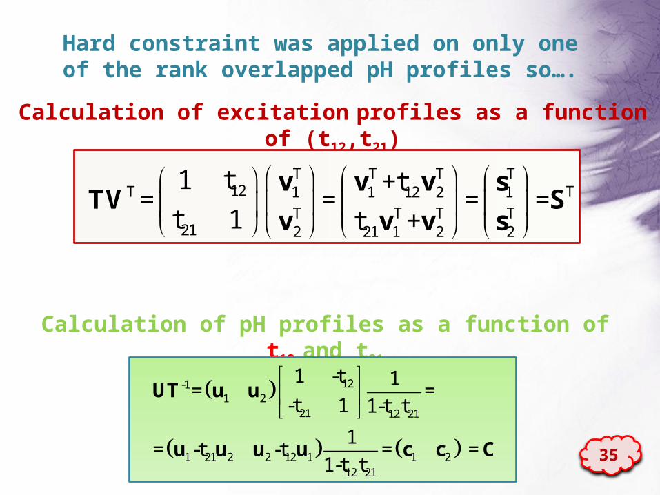
Calculation of excitation profiles as a function of (t12,t21)

Calculation of pH profiles as a function of t12

and t21

T T T T12T T1 1 12 2 1

T T T T21 2 21 1 2 2

1 t +t= = = =

t 1 t +

v v v sTV S

v v v s

12-11 2

21 12 21

1 21 2 2 12 1 1 212 21

1 -t 1= =

-t 1 1-t t

1= -t -t = =

1-t t

UT u u

u u u u c c C 35

Hard constraint was applied on only one of the rank overlapped pH profiles so….

Hard constraints have been applied on rank overlap components.

Results of PARAFAC and HSPARAFAC for Case IIIa Three-way Data

HA A- +H+

HB B- +H+

All components are Spectroscopic active

emHA=emA-

Unique Time(s)Iter. Iter.Methods

Free Noise Data Noisy Data

5.00839 12.09 421 6.15

Time(s) pKapKa

4.00

Rank overlap and closure rank deficiency

PARAFAC

HSPARAFAC .7508 62.78 2650 21.89

36

Results of PARAFAC and HSPARAFAC for Case IIIb Three-way Data

HA A- +H+

HB B- +H+

All components are Spectroscopic active

emHA=emHB

Unique Time(s)Iter. Iter.Methods

Free Noise Data Noisy Data

5.001398 19.21 991 16.01

Time(s) pKapKa

5.00

Rank overlap and closure rank deficiency

PARAFAC

HSPARAFAC ?

Hard constraints has been applied on one of the rank overlap components. 37

There were not good initialization for rank overlap species

Results of PARAFAC, HSPARAFAC and HPARAFAC for Case IIIc Three-way Data

HA A- +H+

HB B- +H+

All components are Spectroscopic activeemHA=emA-

emHB=emB-

Unique Time(s)Iter. Iter.Methods

Free Noise Data Noisy Data

Time(s) pKapKa

Rank overlap and twoclosure rank deficiency

PARAFAC&

HSPARAFAC

HPARAFAC 5.00763 13.62 371 7.135.00.

38

Spectroflurimetric study of acid-base

equilibria of Pyridoxine

H2A HA- + H+

HA- A- 2 + H+

39

250

300

350400

450

200

400

600

800

250

300

350400

450

200

400

600

250

300

350400

450

200

400

600

250

300

350400

450

200400600

800

λem. λex λem. λex

λem. λex λem.λex

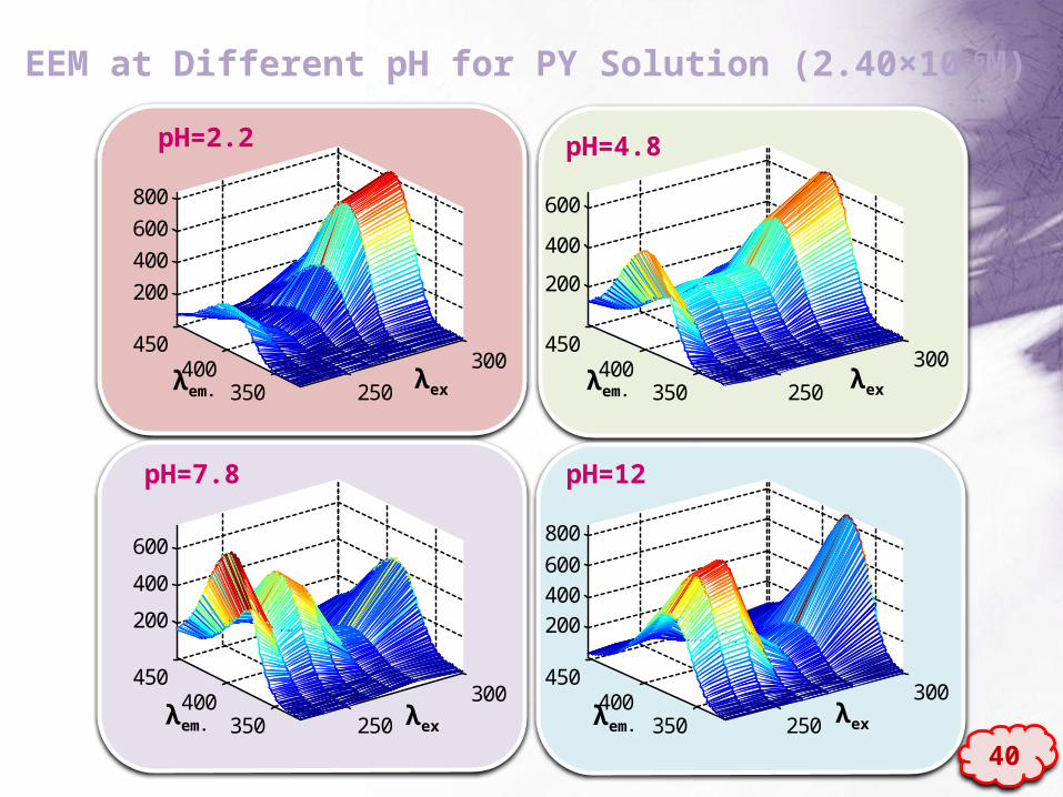
pH=2.2 pH=4.8

pH=7.8 pH=12

EEM at Different pH for PY Solution (2.40×10-6M)

40

41

42

43

pKa2 pKa1 Time No. of iter. Method

7.58 1410 PARAFAC

9.09 4.81 1.03 68 HSPARAFAC

9.05 4.81 0.32 13 HPARAFAC

Reported pKa1 and pKa2 of PY are 4.8 and 9.2 respectively.

Ghasemi J, Abbasi B, Kubista M. J. Korean Chem. Soc. 2005; 49: 269-277. 44

Spectrophotometric study of tarterazin and

sunset yellow in mixtures.

45

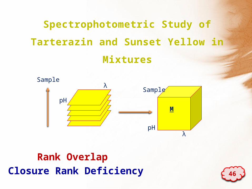
Spectrophotometric Study of

Tarterazin and Sunset Yellow in

Mixtures

M

Sample

pH

Sample

pH

λ

λ

Rank OverlapClosure Rank Deficiency 46

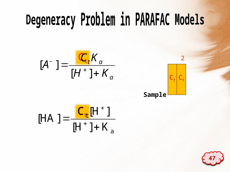
a

t

K]H[

]H[C]HA[

a

at

KH

KCA

][][

Ct Ct

2

Sample

Ct

Ct

47

250 300 350 400 450 500 550 6000

0.02

0.04

0.06

0.08

0.1

0.12

0.14

Abs. Wavelength (nm)

Ab

s.

1 2 3 4 5 6 7 80.1

0.2

0.3

0.4

0.5

0.6

0.7

Sample number

con

cen

tra

tion

(M

icro

mo

lar)

7 7.5 8 8.5 9 9.5 10 10.5 11 11.5 120

0.05

0.1

0.15

0.2

0.25

0.3

0.35

0.4

pH

Re

lativ

e c

on

cen

tra

tion

48

1 2 3 4 5 6 7 8

0.1

0.2

0.3

0.4

0.5

0.6

0.7

Sample number

con

cen

tra

tion

(M

icro

mo

lar)

250 300 350 400 450 500 550 600

0

0.02

0.04

0.06

0.08

0.1

0.12

Abs. Wavelength (nm)

Ab

s.

7 7.5 8 8.5 9 9.5 10 10.5 11 11.5 12

0.05

0.1

0.15

0.2

0.25

0.3

0.35

0.4

pH

Re

lativ

e c

on

cen

tra

tion

49

Method No. of iter. Time pKa1 pKa2

PARAFAC 6548 560.17 - -

HPARAFAC 429 28.15 10.61 9.51

Reported pKa of TA ans SY are 9.6 and 10.4 respectively.

Pérez-Urquiza M, Beltrán JL. Journal of Chromatography A. 2001;917:331-6.

50

Conclusion HSPARAFAC method can decompose data

uniquely when the equilibrium model of rank overlap species are incorporated in the HSPARAFAC algorithm even in the presence of unknown interference.

The parameters of the models, i.e. pKas, were calculated.

Compared with PARAFAC, HSPARAFAC take much less time and the number of iterations greatly reduced.

51

Thanks to Mr. Javad Vallipour from Tabriz University 52

53

54

Please analyze each data with these algorithms to find the advantages of HSPARAFAC rather than PARAFAC !!!

All the mentioned simulated three-way data, the GUI program of PARAFAC, the HSPARAFAC for monoporotic acids are available on the web.