PGE 310: Formulation and Solution of Geosystems Engineering Problems Dr. Matthew T. Balhoff Spring 2011 Notes Adapted from: Chapra, S., Canale, R. “Numerical.

PGE 310: Formulation and Solution of Geosystems Engineering Problems

Dr. Matthew T. Balhoff

Spring 2011

Notes Adapted from:

Chapra, S., Canale, R. “Numerical Methods for Engineers”, Mc-Graw Hill Co. (2010)Rectenwald, G. “Numerical Methods with MATLAB”Prentice-Hall (2000)Gilat, A., Subramaniam, V. “Numerical Methods for Engineers and Scientists” John Wiley and Sons Inc. (2011)

About Me

• Education/Research Experience– B.S. Chemical Engineering, Louisiana State University 2000– Ph.D. Chemical Engineering, Louisiana State University 2005– ICES Postdoctoral Fellow (CSM), UT-Austin 2005-2007– Assistant Professor, UT-Austin 2007-

• Research Interests– Flow and transport in porous media– Non-Newtonian flow– Pore-scale and Multi-scale modeling– NUMERICAL METHODS

+ =

What’s a Numerical Method ?

• Many math problems cannot be solved analytically (exactly)

• Numerical methods are approximate techniques

• Real-life problems in science and engineering require these numerical techniques

• Real world problems can take hours, days, or years to solve. A well written computer program (in MATLAB for example) can do it much faster.

Example 1: Roots of Equations

• A root of an equation is the value that results in a “zero” of the function

• Q: Find the root of the following quadratic equation

2( ) 4 3 0f x x x

Example 1: Roots of Equations

• A root of an equation is the value that results in a “zero” of the function

• Q: Find the root of the following quadratic equation

• A: The quadratic formula is an EXACT method for solving the roots of a quadratic equation

• Answer can be found by plugging in a, b, and c.

2( ) 4 3 0f x x x

22 4 4 4(1)(3)41,3

2 2(1)

b b acx

a

Example 1. Roots of Equations

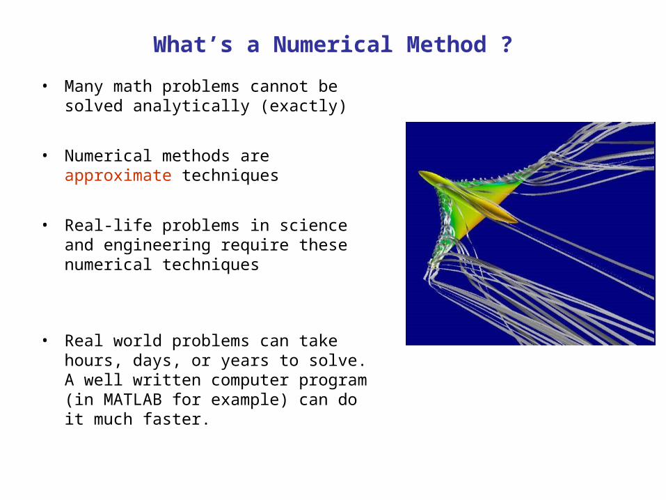
• Ideal gas law doesn’t always apply: iPV RT

Example 1. Roots of Equations

• Ideal gas law doesn’t always apply:

• In petroleum engineering, we deal with gases far from ideal (P=50 bar, T=473K)

iPV RT

2 22i i i

RT aP

V b V bV b

2 20.457

2.3 6

0.077824.7

c

c

c

c

R Ta E

P

RTb

P

Methane

Example 1. Roots of Equations

• Ideal gas law doesn’t always apply:

• In petroleum engineering, we deal with gases far from ideal (P=50 bar, T=473K)

• So how do we find the root of this function, where the quadratic equation doesn’t apply? (R= 83.14 cm3-bar/mol-K)

iPV RT

2 22i i i

RT aP

V b V bV b

2 20.457

2.3 6

0.077824.7

c

c

c

c

R Ta E

P

RTb

P

Methane

2

39325 2.3 6( ) 50 0

24.7 49.4 611i i i

Ef V

V V V

Example 1: Ideas?

• What would be a good guess, if we needed a “ballpark” figure?

Example 1: Ideas?

• What would be a good guess, if we needed a “ballpark” figure?

• How can we get very close to the “exact” solution by performing very few calculations?

83.14 473786.5

50i

RTV

P

Example 1: Ideas?

• What would be a good guess, if we needed a “ballpark” figure?

• How can we get very close to the “exact” solution by performing very few calculations?

83.14 473786.5

50i

RTV

P

2

2

2

2

39325 2.3 6(786) 50 1.87

24.7 49.4 611

39325 2.3 6(750) 50 0.389

24.7 49.4 611

39325 2.3 6(768) 50 0.7518

24.7 49.4 611

39325 2.3 6(759) 50 0.188

24.7 49.4 611

(754.5

i i i

i i i

i i i

i i i

Ef

V V V

Ef

V V V

Ef

V V V

Ef

V V V

f

2

39325 2.3 6) 50 0.0988

24.7 49.4 611i i i

E

V V V

Root ~ 755

Could have plotted points

Example 2. Differentiation

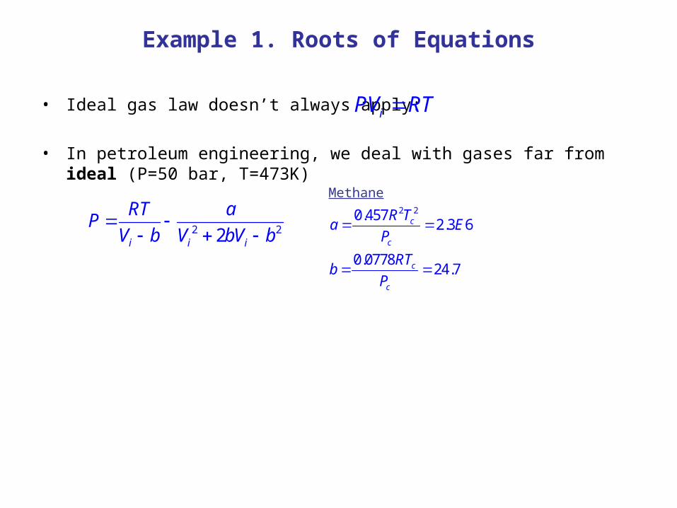
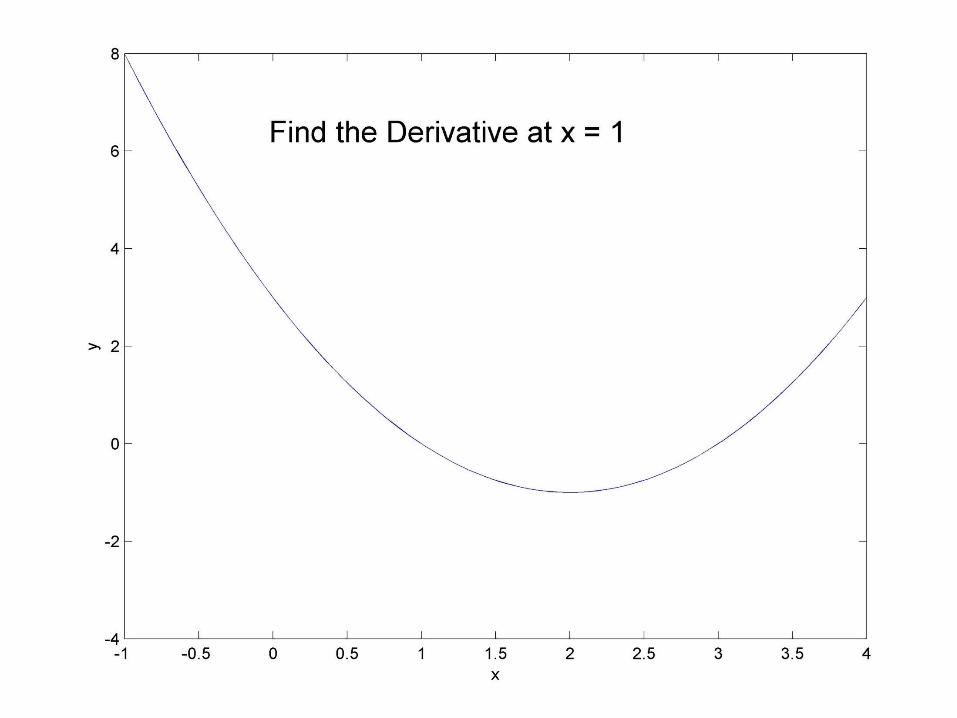
• Derivative: “the slope of the line tangent to the curve”.

• But we seem to forget about that once we learn some fancy tricks to find the derivative

2 4 3y x x

• Q: What is the derivative (dy/dx) at x = 1?

Example 2. Differentiation

• Derivative: “the slope of the line tangent to the curve”.

• But we seem to forget about that once we learn some fancy tricks to find the derivative

342 xxy• Q: What is the derivative (dydx) at x = 1?

42 xdx

dy 24)1(21 xdx

dy

• But how do we find the derivative of a really complicated function – or one that isn’t described by an equation?

dy/dx = slope = -2

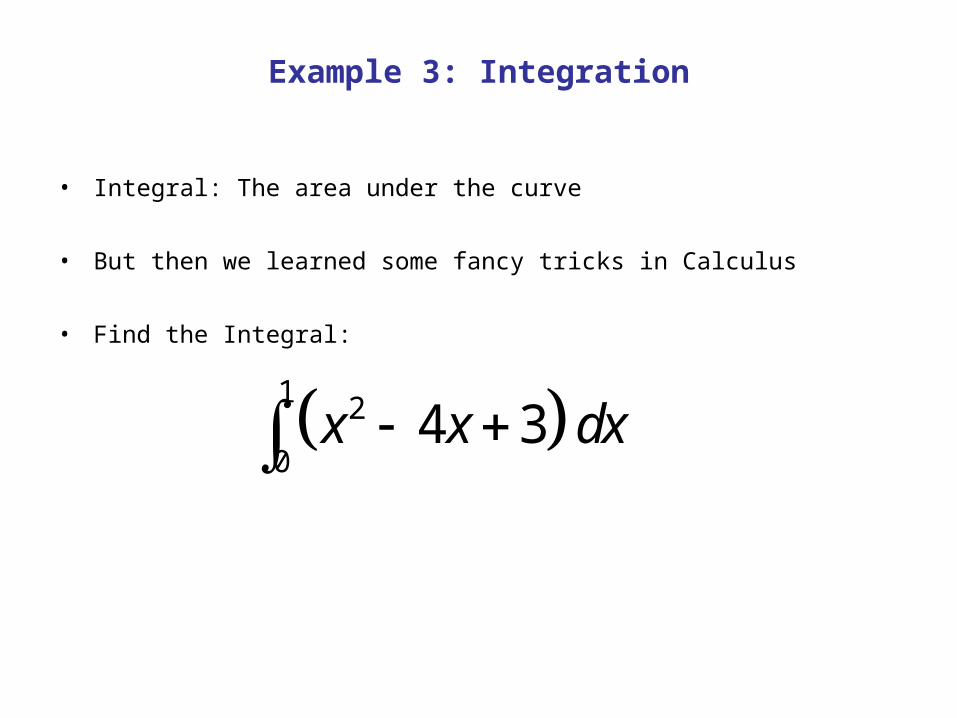
Example 3: Integration

• Integral: The area under the curve

• But then we learned some fancy tricks in Calculus

• Find the Integral:

1 2

04 3x x dx

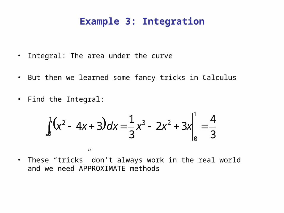
Example 3: Integration

• Integral: The area under the curve

• But then we learned some fancy tricks in Calculus

• Find the Integral:

3

432

3

134

1

0

231

0

2 xxxdxxx

• These “tricks” don’t always work in the real world and we need APPROXIMATE methods

w1 = 1/4

H1 = y(0)Area1 = H1*w1

Add areas of triangles to approximate area under the curve

Area2 = H2*w2

w1 = 1/4

H1 = y(0)Area1 = H1*w1

Add areas of triangles to approximate area under the curve

Area2 = H2*w2

Some error

We get a better answer by using more rectangles

Compare Answers

• 4 Rectangles: Area = 1.7188

• 10 Rectangles: Area= 1.4850

• 100 Rectangles: Area = 1.3484

• 1,000,000 Rectangles = 1.3333

• Actual = 4/3

Great. Now what’s the computer for?

• Numerical methods can require lots of computational effort– Root solving method may take lots of iterations before it converges– We might have to differentiate millions of equations – We might need thousands of little rectangles

• Computers can solve these problems a lot faster if we program them right

• We’ll have to learn some programming (in Matlab) before moving on to learning advanced numerical techniques

• Matlab isn’t hard, it just requires PRACTICE. Don’t get intimidated