Petri Nets in Snoopy: A Unifying Framework for the Graphical Display, Computational Modelling, and Simulation of Bacterial Regulatory Networks

Marwan, Rohr, Heiner Petri nets in Snoopy

Petri nets in Snoopy: A unifying frame-work for the graphical display, computationalmodelling, and simulation of bacterial regu-latory networks

Wolfgang Marwan1∗, Christian Rohr1,2, Monika Heiner2

1 Otto von Guericke University & Magdeburg Centre for Systems Biology, c/o Max PlanckInstitute for Dynamics of Complex Technical Systems, Sandtorstr. 1, 39106 Magdeburg,Germany.2 Department of Computer Science, Brandenburg University of Technology, Postbox 10 13 44,

03013 Cottbus, Germany.

Email: [email protected], [email protected];

[email protected];

∗Corresponding author

AbstractUsing the example of phosphate regulation in enteric bacteria, we demonstratethe particular suitability of stochastic Petri nets to model biochemical phenom-ena and their simulative exploration by various features of the software toolSnoopy.

keywordsPetri nets, stochastic Petri nets, non-Markovian Petri nets, deterministic delay,animation, Gillespie simulation, stochastic simulation analysis, continuous timeMarkov chain.

1 Introduction1.1 Executable Petri nets as a unifying framework for systems biologySystems biology is based on a transdisciplinary joint effort to understand thecomplex mechanisms of life at the molecular systems level. For good reasons,experimentalists and theoreticians traditionally use different languages specificto their respective disciplines, thinking and expressing themselves in different

Humana Press, Methods in Molecular Biology, Chapter 21 - preprint 1

Marwan, Rohr, Heiner Petri nets in Snoopy

ways. Experimentalists think in molecules and molecular mechanisms, whichthey illustrate with pictures, qualitative schemes, and biochemical reactionpathways. Theoreticians communicate by using equations and mathematicalsymbols, which are difficult to read for the majority of experimentalists, whofrequently do not have any significant mathematical background. A true un-derstanding of each other would be greatly facilitated by establishing a commu-nication platform (and language) which is equally easy to use for both experi-mentalists and theoreticians. Such common language should be of unequivocalexpressiveness and directly refer to the traditional languages of both.

With Snoopy, we provide a tool that supports the use of Petri nets as

• a common communication platform (modelling language) for experimen-talists and theoreticians, together with

• a unifying framework for the graphical display, computational modelling,simulation, and bioinformatic annotation of biochemical networks, suchas bacterial regulatory networks.

Petri nets as executable models. A Petri net is a mathematical graphwith a strictly defined syntax. A Petri net is directly executable, if it is rep-resented with the help of an appropriate tool like Snoopy. Snoopy translatesautomatically and thus reproducibly the graphical scheme into a set of equationsused by the program to run simulations. In other words, a graphical represen-tation of a Petri net drawn in Snoopy can be executed, i.e. simulations can berun with a mouse click; no special additional encoding is required.

Petri nets represent molecular and other mechanisms with a strictlydefined syntax. The syntax of the Petri net language is simple and thereforevery easy to learn (see below). Because the syntax is strictly defined, there isno ambiguity in what a graphical representation of the Petri net model meansin terms of reaction mechanism. The Petri net formalism is ideal to naturallyrepresent chemical reactions and their mechanisms, and any type of biochem-ical interactions. As defined by the user, Petri net components may representmolecules and reactions, or even more complex entities and processes. Thisallows to describe and represent biological processes at arbitrary level of ab-straction (i.e. with arbitrary resolution in detail), but always mechanisticallyunambiguous, and to join those processes into a coherent, executable model.This option is extremely useful for signal transduction networks or gene regula-tory networks as usually not all processes involved in a phenomenon of interestare and will be known with the same resolution in detail.

Petri nets provide a unifying framework for modelling and sim-ulation in systems biology. Petri nets can be used to perform all majormodelling and simulation approaches central to systems biology. Briefly,thereare several reasons suggesting the deployment of Petri nets to investigate bio-chemical networks.

1. Petri nets [1] enjoy an intuitive bipartite graphical representation, whichmakes them easily comprehensible and facilitates the communication be-tween wet-lab experimentalists and computational theoreticians.

Humana Press, Methods in Molecular Biology, Chapter 21 - preprint 2

Marwan, Rohr, Heiner Petri nets in Snoopy

2. Petri nets allow the unambiguous representation of various types of biolog-ical processes at different levels of abstraction (with different resolution ofdetail) in one and the very same model ranging from the conformationalchange of a single molecule to the macroscopic response of a cell [2], thedevelopment of a tissue, or even the behaviour of a whole organism; for arecent survey of case studies employing Petri nets see [3].

3. Petri nets come along with an explicit notion of concurrency. This allowsto distinguish unmistakably between alternative and concurrent behaviourand means an adequate representation of inherently concurrent behaviour,such as the concurrent dephosphorylation in the individual stages of asignalling cascade [4] (see also Note 2).

4. Petri nets are directly executable by an appropriate tool like Snoopy [5].This execution allows a time-free animation in the case of qualitative Petrinets (these are the standard Petri nets), and time-dependent animationand simulation in the case of quantitative Petri nets (in our case, stochasticPetri nets).

5. Petri nets can be explored by a substantial body of mathematically foundedanalysis techniques, covering structural and behavioural properties as wellas their relations [4,6]; see also Notes 3-5.

6. Petri nets may serve as a kind of umbrella formalism integrating quali-tative and quantitative (i.e. stochastic, continuous, or hybrid) modellingand analysis techniques. A related unifying framework is demonstrated in[4,6].

7. Petri nets in all their flavours and related analysis techniques are sup-ported by several reliable tools, developed by an international communityof computer scientists [7-10].

As we will show below, Snoopy provides several features that allow to com-fortably handle large, complex models.

2 Material2.1 SoftwareIn this chapter we use Snoopy [5], a software tool to design and animate or sim-ulate hierarchical graphs, among them the Petri net classes: standard Petri nets(PN), extended Petri nets (xPN), and extended stochastic Petri nets (xSPN).The Snoopy software has three distinguished features.

1. It is extensible; its generic design facilitates the implementation of newgraph types.

2. It is adaptive by supporting the simultaneous use of several graph types,while the GUI adopts dynamically to the graph type in the active window.

Humana Press, Methods in Molecular Biology, Chapter 21 - preprint 3

Marwan, Rohr, Heiner Petri nets in Snoopy

3. It is platform-independent. The tool runs on Mac OS X, Windows, andLinux.

The software is freely available for non-profit academic research purposes athttp://www-dssz.informatik.tu-cottbus.de/software/snoopy.html.

2.2 File formatsPetri nets which have been designed with Snoopy can be saved and reloadedin a Snoopy-specific file format applying XML technology. The file formatsvary slightly for the individual Petri net classes and are typically indicated byspecific file extensions, such as spped (PN), spept (xPN), spstochpn (xSPN).Snoopy offers build-in animation and stochastic simulation, which are used inthis chapter.

Supplementary, Snoopy provides continuous simulation of continuous Petrinets and export to various analysis tools as well as import and export of thestandard exchange format SBML, Level 2, Version 3 (http://sbml.org). ThePetri nets and simulation plots can be saved in Encapsulated Postscript (eps)format as well. For more information see Snoopy’s website, and Notes 3, 4.

2.3 Sample filesAll Petri nets used in this chapter are available at http://www-dssz.informatik.tu-cottbus.de/examples/mimb/. To repeat the computational experimentsdiscussed in this chapter, you just need to download Snoopy, to open theseexample files, and to follow the steps described in the Methods section.

3 MethodsIn this section we describe briefly three net classes and the main features oftheir animation and simulation, which will later be used to perform the casestudy, the phosphate network of enteric bacteria. See also Note 1.

3.1 Petri nets (PN)The standard notion of Petri nets does not involve any timing aspects. Thosenets are purely qualitative, i.e. time-free models. Technically speaking, Petrinets are weighted, directed, bipartite graphs which consist of the following basicingredients (compare Figures 1-2).

1. There are two types of nodes, which are called places, graphically repre-sented by circles, and transitions, graphically represented by rectangles.Places usually model passive system components like species (substrates)playing the role of precursors and products of chemical reactions, whiletransitions stand for active system components like chemical reactions,transforming precursors into products or simply transporting species from

Humana Press, Methods in Molecular Biology, Chapter 21 - preprint 4

Marwan, Rohr, Heiner Petri nets in Snoopy

!"#$%

&'#()*+*,(

&,-%(

.'$

/%#01.'$

2(3*4*+,'51.'$

!%+'*16%+)

6,0%)17,'18'#93*$#"1:*)9"#5

,71;#'<%'1!%+'*16%+)

6,0%)

=0<%)1

,'1

.'$)

=>+%(0%01!%+'*16%+)

;,<*$#"

6,0%)

?#$',1

6,0%)

;,<*$#"1!"#$%

;,<*$#"1&'#()*+*,(

?#$',1!"#$%

?#$',1&'#()*+*,(

?#'-*(<

?,0*7*%'1

.'$

&*@%0

&'#()*+*,()

=>+%(0%01A+,$3#)+*$1!%+'*16%+)

A+,$3#)+*$1&'#()*+*,(

:%+%'@*(*)+*$BA$3%0C"%0

2@@%0*#+%1&'#()*+*,(

&'#()*+*,(

Figure 1: Petri net elements and their graphical representation. Petri nets areweighted, directed, bipartite graphs consisting of nodes and arcs. The nodesof a Petri net, the places and transitions, are interconnected by arcs. An arcalways connects a place with a transition or vice versa, but never two places ortwo transitions with each other. Places may contain (be marked with) tokens,while transitions can not contain any tokens. Standard Petri nets are composedof places, transitions and (standard) arcs. The other Petri net components areintroduced in the text.

Humana Press, Methods in Molecular Biology, Chapter 21 - preprint 5

Marwan, Rohr, Heiner Petri nets in Snoopy

Figure 2: Some typical basic structures of biochemical networks. (a) formationand decay of a macro-molecular complex; (b) reversible reactions; (c) sequentialreactions; (d) alternative reactions; (e) concurrent, i.e. independent reactions.

a site A to a site B. Reversible chemical reactions are modelled by twoopposite transitions (see Figure 2-b). Due to their strong correspondence,we often use the two terms ’transition’ and ’reaction’ interchangeably.

2. The directed arcs (edges) connect always nodes of different type. Theygo from precursors to reactions, and from reactions to products. In otherwords, the pre-places of a transition correspond to the reactions precur-sors, and its post-places to the reactions products.

3. Arcs are weighted by natural numbers. The arc weight may be read as themultiplicity of the arc, reflecting known stoichiometries or other semi-quantitative assumptions. The arc weight 1 is the default value and isusually not given explicitly.

4. A place carries an arbitrary amount of tokens, represented as black dotsor a natural number. The number zero is the default value and usuallynot given explicitly. Tokens can be interpreted as the available amount ofa given species in number of molecules or any abstract, i.e. discrete con-centration level. The tokens on all places establish together the markingof the net, which represents the current state of the system.

Humana Press, Methods in Molecular Biology, Chapter 21 - preprint 6

Marwan, Rohr, Heiner Petri nets in Snoopy

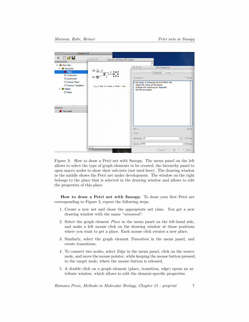
Figure 3: How to draw a Petri net with Snoopy. The menu panel on the leftallows to select the type of graph elements to be created, the hierarchy panel toopen macro nodes to show their sub-nets (not used here). The drawing windowin the middle shows the Petri net under development. The window on the rightbelongs to the place that is selected in the drawing window and allows to editthe properties of this place.

How to draw a Petri net with Snoopy. To draw your first Petri netcorresponding to Figure 3, repeat the following steps.

1. Create a new net and chose the appropriate net class. You get a newdrawing window with the name “unnamed“.

2. Select the graph element Place in the menu panel on the left-hand side,and make a left mouse click on the drawing window at those positionswhere you want to get a place. Each mouse click creates a new place.

3. Similarly, select the graph element Transition in the menu panel, andcreate transitions.

4. To connect two nodes, select Edge in the menu panel, click on the sourcenode, and move the mouse pointer, while keeping the mouse button pressed,to the target node, where the mouse button is released.

5. A double click on a graph element (place, transition, edge) opens an at-tribute window, which allows to edit the element-specific properties.

Humana Press, Methods in Molecular Biology, Chapter 21 - preprint 7

Marwan, Rohr, Heiner Petri nets in Snoopy

6. Finally, do not forget to save your work under a new name (File → Saveas).

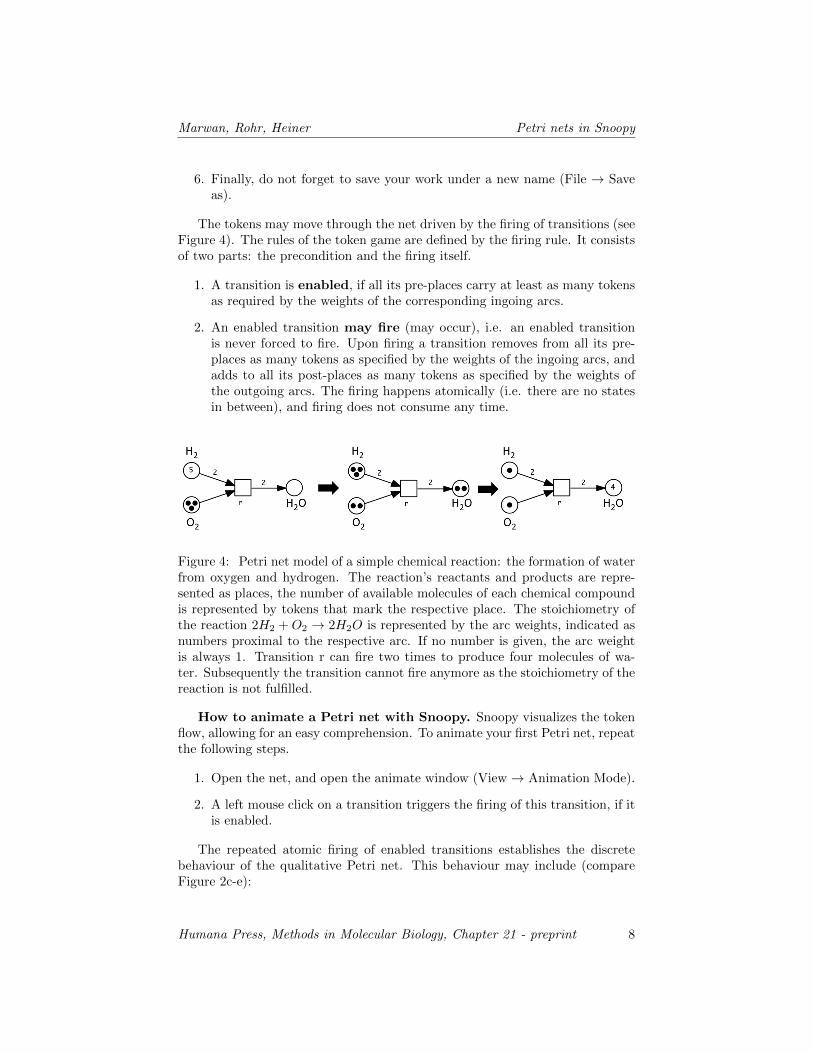
The tokens may move through the net driven by the firing of transitions (seeFigure 4). The rules of the token game are defined by the firing rule. It consistsof two parts: the precondition and the firing itself.

1. A transition is enabled, if all its pre-places carry at least as many tokensas required by the weights of the corresponding ingoing arcs.

2. An enabled transition may fire (may occur), i.e. an enabled transitionis never forced to fire. Upon firing a transition removes from all its pre-places as many tokens as specified by the weights of the ingoing arcs, andadds to all its post-places as many tokens as specified by the weights ofthe outgoing arcs. The firing happens atomically (i.e. there are no statesin between), and firing does not consume any time.

Figure 4: Petri net model of a simple chemical reaction: the formation of waterfrom oxygen and hydrogen. The reaction’s reactants and products are repre-sented as places, the number of available molecules of each chemical compoundis represented by tokens that mark the respective place. The stoichiometry ofthe reaction 2H2 + O2 → 2H2O is represented by the arc weights, indicated asnumbers proximal to the respective arc. If no number is given, the arc weightis always 1. Transition r can fire two times to produce four molecules of wa-ter. Subsequently the transition cannot fire anymore as the stoichiometry of thereaction is not fulfilled.

How to animate a Petri net with Snoopy. Snoopy visualizes the tokenflow, allowing for an easy comprehension. To animate your first Petri net, repeatthe following steps.

1. Open the net, and open the animate window (View → Animation Mode).

2. A left mouse click on a transition triggers the firing of this transition, if itis enabled.

The repeated atomic firing of enabled transitions establishes the discretebehaviour of the qualitative Petri net. This behaviour may include (compareFigure 2c-e):

Humana Press, Methods in Molecular Biology, Chapter 21 - preprint 8

Marwan, Rohr, Heiner Petri nets in Snoopy

1. sequential reactions reflecting causality (e.g., reaction r5 can not happenbefore r4 happened);

2. alternative reactions competing for tokens on shared pre-places and there-fore branching into alternative behaviour; in Petri net terminology, thetransitions are said to be in conflict (e.g., reactions r6 and r7 share thepre-place L; a token on L can either be consumed by r6 or by r7);

3. concurrent reactions, which are neither in causal nor conflict relation;thus, they are independent and can fire in any order or even concurrently(e.g., reactions r8 and r9).

In addition to a basic toolkit for drawing Petri nets, Snoopy supports twodistinguished features for the design and systematic construction of larger Petrinets (see Figures 1 and 5).

1. Places and transitions can be specified as logical nodes (also called fusionnodes). They are automatically coloured in grey. Logical nodes with thesame name are identical, i.e., graphical copies of a single node (placeor transition). They are often used for compounds involved in severalreactions or reactions involving distributed compounds.

2. There are two types of macro nodes. Macro transitions (drawn as twocentric squares) help to hide transition-bordered subnets (i.e. subnetshaving only transitions as interface to the super-net). Likewise, macroplaces (drawn as two centric circles) can be used to hide place-boundedsubnets (i.e. subnets having only places as interface to the super-net).Both types of macro nodes allow a hierarchical structuring of Petri nets.

Logical nodes and macro nodes help to deal with larger networks. Theymay contribute to a net’s readability and, therefore, are crucial for non-trivialnet examples. However, they do not extend the expressiveness of the modellinglanguage. Contrary, the features introduced in the next section do extend theexpressiveness.

How to draw an hierarchical Petri net with Snoopy. To hierarchicallystructure a Petri net, repeat the following steps.

1. Draw your flat net (or portion of it) as you wish to have it.

2. Select the sub-graph which you want to be abstracted by a macro node,and select Hierarchy→ Coarse. Chose the appropriate coarse element andhit the OK button.

3. A double click on the macro node opens its attribute window and allows toassign a suitable name, a click on the entry with this name in the hierarchypanel on the left-hand side opens the sub-graph in a separate window.The blue net parts have been automatically generated and represent theconnection of the sub-graph (macro node) with the neighbouring nodeson the next higher hierarchy level.

Humana Press, Methods in Molecular Biology, Chapter 21 - preprint 9

Marwan, Rohr, Heiner Petri nets in Snoopy

4. Finally, do not forget to save your work under a new name (File → Saveas).

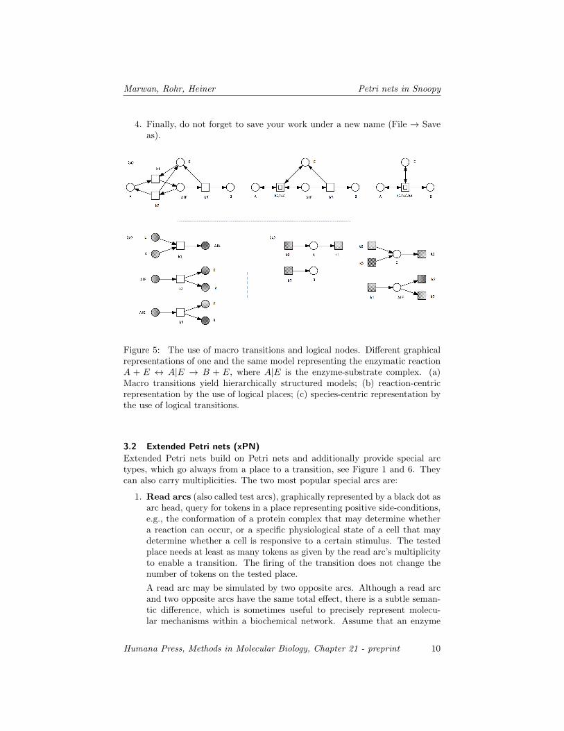
Figure 5: The use of macro transitions and logical nodes. Different graphicalrepresentations of one and the same model representing the enzymatic reactionA + E ↔ A|E → B + E, where A|E is the enzyme-substrate complex. (a)Macro transitions yield hierarchically structured models; (b) reaction-centricrepresentation by the use of logical places; (c) species-centric representation bythe use of logical transitions.

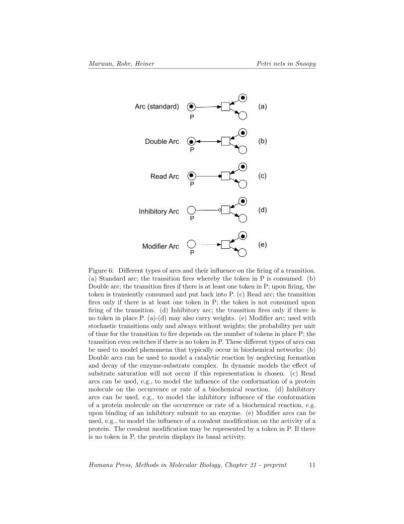
3.2 Extended Petri nets (xPN)Extended Petri nets build on Petri nets and additionally provide special arctypes, which go always from a place to a transition, see Figure 1 and 6. Theycan also carry multiplicities. The two most popular special arcs are:

1. Read arcs (also called test arcs), graphically represented by a black dot asarc head, query for tokens in a place representing positive side-conditions,e.g., the conformation of a protein complex that may determine whethera reaction can occur, or a specific physiological state of a cell that maydetermine whether a cell is responsive to a certain stimulus. The testedplace needs at least as many tokens as given by the read arc’s multiplicityto enable a transition. The firing of the transition does not change thenumber of tokens on the tested place.

A read arc may be simulated by two opposite arcs. Although a read arcand two opposite arcs have the same total effect, there is a subtle seman-tic difference, which is sometimes useful to precisely represent molecu-lar mechanisms within a biochemical network. Assume that an enzyme

Humana Press, Methods in Molecular Biology, Chapter 21 - preprint 10

Marwan, Rohr, Heiner Petri nets in Snoopy

Arc (standard)

Double Arc

Read Arc

Inhibitory Arc

Modifier Arc

!

""

""

""

""

""

""

""

"

!

""

""

""

""

""

""

""

"

!

""

""

""

""

""

""

""

"

!

""

""

""

""

""

""

""

"

!

""

""

""

""

""

""

""

"

(a)

(b)

(c)

(e)

(d)

Figure 6: Different types of arcs and their influence on the firing of a transition.(a) Standard arc; the transition fires whereby the token in P is consumed. (b)Double arc; the transition fires if there is at least one token in P; upon firing, thetoken is transiently consumed and put back into P. (c) Read arc; the transitionfires only if there is at least one token in P; the token is not consumed uponfiring of the transition. (d) Inhibitory arc; the transition fires only if there isno token in place P. (a)-(d) may also carry weights. (e) Modifier arc; used withstochastic transitions only and always without weights; the probability per unitof time for the transition to fire depends on the number of tokens in place P; thetransition even switches if there is no token in P. These different types of arcs canbe used to model phenomena that typically occur in biochemical networks: (b)Double arcs can be used to model a catalytic reaction by neglecting formationand decay of the enzyme-substrate complex. In dynamic models the effect ofsubstrate saturation will not occur if this representation is chosen. (c) Readarcs can be used, e.g., to model the influence of the conformation of a proteinmolecule on the occurrence or rate of a biochemical reaction. (d) Inhibitoryarcs can be used, e.g., to model the inhibitory influence of the conformationof a protein molecule on the occurrence or rate of a biochemical reaction, e.g.upon binding of an inhibitory subunit to an enzyme. (e) Modifier arcs can beused, e.g., to model the influence of a covalent modification on the activity of aprotein. The covalent modification may be represented by a token in P. If thereis no token in P, the protein displays its basal activity.

Humana Press, Methods in Molecular Biology, Chapter 21 - preprint 11

Marwan, Rohr, Heiner Petri nets in Snoopy

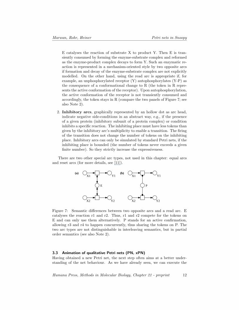
E catalyses the reaction of substrate X to product Y. Then E is tran-siently consumed by forming the enzyme-substrate complex and reformedas the enzyme-product complex decays to form Y. Such an enzymatic re-action is represented in a mechanism-oriented style by two opposite arcsif formation and decay of the enzyme-substrate complex are not explicitlymodelled. On the other hand, using the read arc is appropriate if, forexample, an unphosphorylated receptor (Y) autophosphorylates (Y-P) asthe consequence of a conformational change to R (the token in R repre-sents the active conformation of the receptor). Upon autophosphorylation,the active conformation of the receptor is not transiently consumed andaccordingly, the token stays in R (compare the two panels of Figure 7; seealso Note 2).

2. Inhibitory arcs, graphically represented by an hollow dot as arc head,indicate negative side-conditions in an abstract way, e.g., if the presenceof a given protein (inhibitory subunit of a protein complex) or conditioninhibits a specific reaction. The inhibiting place must have less tokens thangiven by the inhibitory arc’s multiplicity to enable a transition. The firingof the transition does not change the number of tokens on the inhibitingplace. Inhibitory arcs can only be simulated by standard Petri nets, if theinhibiting place is bounded (the number of tokens never exceeds a givenfinite number). So they strictly increase the expressiveness.

There are two other special arc types, not used in this chapter: equal arcsand reset arcs (for more details, see [11]).

X1 Y1

E

X2 Y2 Y2X2

P

Y1X1(a) (b)

Figure 7: Semantic differences between two opposite arcs and a read arc. Ecatalyses the reaction r1 and r2. Thus, r1 and r2 compete for the tokens onE and can only use them alternatively. P stands for an active confirmation,allowing r3 and r4 to happen concurrently, thus sharing the tokens on P. Thetwo arc types are not distinguishable in interleaving semantics, but in partialorder semantics (see also Note 2).

3.3 Animation of qualitative Petri nets (PN, xPN)Having obtained a new Petri net, the next step often aims at a better under-standing of the net behaviour. As we have already seen, we can execute the

Humana Press, Methods in Molecular Biology, Chapter 21 - preprint 12

Marwan, Rohr, Heiner Petri nets in Snoopy

Petri net by playing the token game to experience the net behaviour. Each exe-cution exemplifies some possible net behaviour. The animation can be triggeredmanually by clicking on an enabled transition. It can also be done in automaticmode by clicking on the control panel. In each step of the automatic modethe set of all enabled transitions is determined. There are three strategies tochoose the transition(s) to be fired in the next execution step among all enabledtransitions.

1. Single step – one single transition is randomly chosen.

2. Intermediate step – an arbitrary subset of concurrent transitions israndomly chosen.

3. Maximal step – a maximal set of concurrent transitions is randomlychosen.

Steps just done can be played backwards up to a depth of 10; this defaultvalue can be changed in the Global Preferences dialogue.

By playing the token game, we can produce and observe any reachable state.All states, which can be reached from a given state by any firing sequence ofarbitrary length, constitute the set of reachable states. Each execution run of anxPN corresponds to a walk through the state space defined by this xPN. The setof states reachable from the initial state is said to be the state space of a givensystem. Often, this qualitative state space is infinite, caused by consideringall possible behaviour of a structurally unbounded Petri net under any timingconstraints. We call a Petri net bounded, if the number of tokens on all placesis bounded by a constant independently of what happens. Then we get a finitestate space, which however can still be too huge to be explored exhaustively.

Executing a Petri net generally needs to make decisions between alternativebehaviour. Encountered alternatives (conflicts) are taken non-deterministically(automatic mode) or user-guided (manual mode). To get an exhaustive picture,we have to consider all possible execution sequences. Obviously, that’s notpossible for systems with infinite behaviour, which can be caused by cyclicbehaviour and/or infinite state space. Thus we have to confine ourselves to asubset of execution sequences, which are considered to be representative.

In the next section we will introduce time and we will see how specific ki-netic assumptions will typically restrict the qualitatively infinite state space toa quantitatively finite state space, if we are only interested in states with aprobability above a certain threshold.

How to change the net class in Snoopy. A (qualitative) Petri net canbe converted into a stochastic Petri net, which allows to re-use the structure.Only the additional attributes have to be set.

1. Open the qualitative Petri net, and go to the export Window (File →Export), chose the appropriate target(s) and hit the OK button.

2. Open the stochastic Petri net, just generated. It looks exactly the sameas the qualitative net.

Humana Press, Methods in Molecular Biology, Chapter 21 - preprint 13

Marwan, Rohr, Heiner Petri nets in Snoopy

Now you are ready to specify the attributes specific for stochastic Petri nets,which are discussed in the next section.

3.4 Stochastic Petri nets (SPN)Stochastic Petri nets build on standard Petri nets. As in the qualitative case,a stochastic Petri net maintains a discrete number of tokens on its places. Butcontrary to the time-free case, a stochastic firing rate is associated with eachtransition, determining a stochastic waiting time before an enabled transitionactually fires, provided it did not loose its license to fire in between. The waitingtimes are random variables following an exponential probability distribution(with the parameter lambda). Therefore, all transition firing sequences of thequalitative Petri net can theoretically still occur, but the probability dependson the individual firing rates of the transitions involved (see Figure 8). Snoopyprovides the following features to specify state-dependent firing rates (i.e. ofthe parameter lambda of the exponential probability distribution).

1. Rate functions are arbitrary mathematical functions, which are storedin lookup tables, if necessary. However, to keep a close relation to thenet structure, only the transition pre-places are allowed as variables in thetransition rate function. Popular kinetics (mass-action semantics, levelsemantics, see [4]) are supported by pre-defined function patterns. Ofcourse, each transition gets its own rate function, making up together alist of rate functions. Moreover, several of such rate functions lists can bemaintained, allowing for quite flexible models.

2. Parameters, in figures represented by ellipses, are real-valued constants,which are used for the rate functions. Parameters can be collected in macroparameter nodes, in figures represented as two centric ellipses. Again,several sets of parameters can be maintained.

3. Modifiers are particular arcs, in figures represented by dashed lines,which always go from a place to a transition. Pre-places connected witha transition by a modifier arc may modify the transition’s firing rate, butdo not have an influence on the transition’s enabledness (contrary to thespecial arcs).

The firing itself of a stochastic transition does not consume time and fol-lows the standard firing rule of qualitative Petri nets. Stochastic Petri netswith exponentially distributed firing delays for all transitions fulfil the Markovproperty; thus their semantics is described by a continuous time Markov chain(CTMC); see [4] for more details. However, in this chapter we confine ourselvesto simulative approaches. Each simulation run of an SPN corresponds to a walkthrough the CTMC defined by this SPN, see Subsection 3.6.

Humana Press, Methods in Molecular Biology, Chapter 21 - preprint 14

Marwan, Rohr, Heiner Petri nets in Snoopy

!"#$%$#&"#%#"'()*$+

v%,%k-

.*#/)%$#&"#%#"'()*$+

v%,%k0%123

4"($+&%$#&"#%#"'()*$+

v%,%k5%123%163

78*#&%$#&"#%#"'()*$+

v%,%k9%123%163%1:3

Figure 8: Automatic generation of reaction rate equations with stochastictransitions in extended stochastic Petri nets. Using the MassAction function,Snoopy automatically generates the correct reaction rate equation dependingon whether a reaction is zero, first, second, or third order. Here, [x] stands forthe concentration of the place x in the case of continuous Petri nets, and for thenumber of tokens on x in the case of stochastic Petri nets.

Humana Press, Methods in Molecular Biology, Chapter 21 - preprint 15

Marwan, Rohr, Heiner Petri nets in Snoopy

3.5 Extended Stochastic Petri nets (xSPN)Extended stochastic Petri nets combine stochastic Petri nets with the specialarc types of extended Petri nets. Additionally, there are deterministically timedtransitions, which come in three flavours.

1. Deterministic transitions have contrary to stochastic transitions – adeterministic firing delay which is specified by an integer constant. Thedelay is always relative to the time point where the transition gets enabled.The transition may lose its enabledness while waiting for the delay toexpire. Then, the transition will not fire. This behaviour is also knownas the so-called pre-emptive firing rule. As for stochastic transitions, thefiring itself of a deterministic transition does not consume time and followsthe standard firing rule of qualitative Petri nets. Deterministic transitionsmay be useful to reduce networks, and thus speed-up simulations, e.g. byreplacing a linear sequence of stochastic transitions by one deterministictransition with the delay set to the expectation value of the sum of thesequence.

2. Immediate transitions are a popular special case of deterministic tran-sitions. They have a zero delay and always highest priority. The lattercreates a subtle difference between an immediate transition and a deter-ministic transition with zero firing delay: if there is a conflict betweenthe two, .i.e. a situation, where two transitions compete for tokens, theimmediate transition gets priority. Immediate transitions may help toavoid stiff systems by using them for transitions with extremely high rates(non-significant delay), compared to the other transitions in the system.

3. Scheduled transitions are another special case of deterministic transi-tions. The deterministic firing occurs according to a schedule specifyingabsolute points of the simulation time. A schedule can specify just asingle time point, or equidistant time points within a given interval, trig-gering the firing once or periodically. However, transitions only fire attheir scheduled time points if they are enabled at this time. Scheduledtransitions can dramatically restrict the (qualitative) net behaviour. Thecrucial point is that they allow to disturb the core model at well-definedtime points as it is done experimentally with the actual biological systemunder investigation in the wet-lab.

An unrestricted use of deterministic transitions destroy the Markov prop-erty, which precludes an analytical evaluation by constructing and analysing theCTMC. If we consider stochastic Petri nets without deterministic transitions,the probability of two transitions to fire at the same time is practically zero.Contrary, in stochastic Petri nets with deterministic transitions, it is possiblethat two transitions want to fire simultaneously. To analyse such a system, allpossible choices have to be considered, while in the simulation a random choicetakes place, see next section (for more details and related examples see [12]).

Humana Press, Methods in Molecular Biology, Chapter 21 - preprint 16

Marwan, Rohr, Heiner Petri nets in Snoopy

In most practical cases, extended stochastic Petri nets are the obvious choice.Therefore, Snoopy does not distinguish between stochastic Petri nets (SPN) andextended stochastic Petri nets (xSPN).

3.6 Simulation of quantitative Petri nets (SPN, xSPN)The simulation of stochastic Petri nets can be read as a timed version of the qual-itative token game, taking into account the stochastic and deterministic delaysof enabled transitions. Snoopy builds upon the Gillespie algorithm [13]. Thisexact method does a step-by-step simulation of possible states of the stochasticPetri net. Consequently, the result represents always a valid state of the un-derlying stochastic process at any time point of the simulation. The standardstochastic simulation algorithm works in the following way:

1. Initialise the SPN network with the chosen initial marking.

2. Calculate the firing rates of all enabled transitions using their rate func-tions.

3. Calculate the combined rate by summing up all transition rates.

4. Determine the time interval until the next state change takes place. Thisis done by computing an exponentially distributed random number de-pending on the current combined transition rate of the net.

5. Increase the simulation time by this time interval.

6. Determine the next system state change. For this purpose, a weightedrandom selection of the transition is made which gets the license to fire.

7. Let the selected transition fire and update the marking of the SPN.

8. Go back to step 2, if the simulation time has not yet reached its end point.

The simulation of xSPN requires some straightforward modifications of thestandard simulation algorithm. Deterministic transitions require a higher pri-ority than stochastic transitions to ensure their correct handling. Immediatetransitions need to have the highest priority (over deterministic and scheduledtransitions) because they have to fire instantaneously when they get enabled.Consequently, the simulation algorithm has to check for enabled immediatetransitions after any change of the marking. In the case of more than oneenabled immediate transitions, the selection is done randomly, but uniformlydistributed. The system may run into a time deadlock, if always an immediatetransition is enabled. Then, time will not progress anymore. Time deadlocksare an indication of inconsistent time assignments. The user has to take care ofavoiding them.

Deterministic and scheduled transitions are treated differently. If a deter-ministic transition gets enabled, its timer starts running until it expires. If

Humana Press, Methods in Molecular Biology, Chapter 21 - preprint 17

Marwan, Rohr, Heiner Petri nets in Snoopy

the deterministic transition is still enabled, it fires. The timer will be simplyswitched-off, if the transition should have lost in between the enabledness. Thefiring of a transition in conflict does not change the timer value. The sched-uled transitions fire at the specified absolute time points, if they are enabledat that time. Otherwise the intention to fire is not used. All conflicts betweendeterministic and/or scheduled transitions are resolved randomly, by uniformlydistributed selection.

Stochastic animation. The progress of a stochastic simulation run canbe observed in the automatic animation mode, which shows the correspondingtoken flow.

Repeated stochastic simulation. Each simulation run is one possibletrace of state changes over time. Therefore, when doing stochastic simulation,a significant number of simulation runs is usually required to get meaningfulresults. For this purpose the traces of the simulation runs are averaged.

The simulation can be parametrised in four ways.

1. Different sets of markings, rate functions and parameters can be chosen.

2. The simulation time of interest can be specified, specifically the intervalstart and interval end, e.g. from 0 to 100 or from 250 to 300.

3. The number of output step points in the specified simulation interval canbe declared. They define together with the interval start and end valuesthe grid of the recorded simulation data.

4. The number of simulation runs can be specified.

Having started the simulation, the progress bar indicates how far the sim-ulation has been gone until now, and the time consumed by the simulation isdisplayed too.

The user can select one out of three export functions:

1. Direct export: the averaged result of the selected places or transitionsis exported.

2. Single trace export: the result of every simulation run is exportedseparately.

3. Exact trace export: every change of the marking of the selected placesor the transition rates at any time point is exported.

The simulation results can be shown as

1. Table, where each column represents a selected place (transition) andeach row shows the averaged marking (firing times) at one output steppoint.

2. Plot, where each curve stands for one selected place (transition); thex-axis holds the time and the y-axis holds the number of tokens (firingtimes).

Humana Press, Methods in Molecular Biology, Chapter 21 - preprint 18

Marwan, Rohr, Heiner Petri nets in Snoopy

Different tables and plots can be created to switch conveniently betweendifferent views on the simulation results. Each table is characterised by a setof selected places (transitions). If a node was coloured, its corresponding curvegets the same colour in the plot. Simulation plots can also be saved in epsformat.

4 Case study4.1 A case study: the phosphate regulation network in enteric bacteriaLet us now consider the phosphate utilisation gene regulatory network in Es-cherichia coli (see Figure 9 discussed in [14]). Note that this case study is neithermeant as a scientific contribution to the understanding of the gene regulatorynetwork of phosphate utilisation nor does it provide any comprehensive repre-sentation of the knowledge on this subject; for a recent survey see [15]. Instead,the case study is intended to show how a typical biochemical model, a gene

PhoU

PstCPstS

PstBPstA

PhoR

PhoB

PhoR P

PhoB P

No geneactivation

Pi

PiPhoU*

PstCPstS

PstBPstA

PhoR

PhoB

PhoR P

PhoB P

Gene activation

No Pi

phoA psiB psiE etc.

Alkalinephosphatase

Other proteinproducts ofthe network

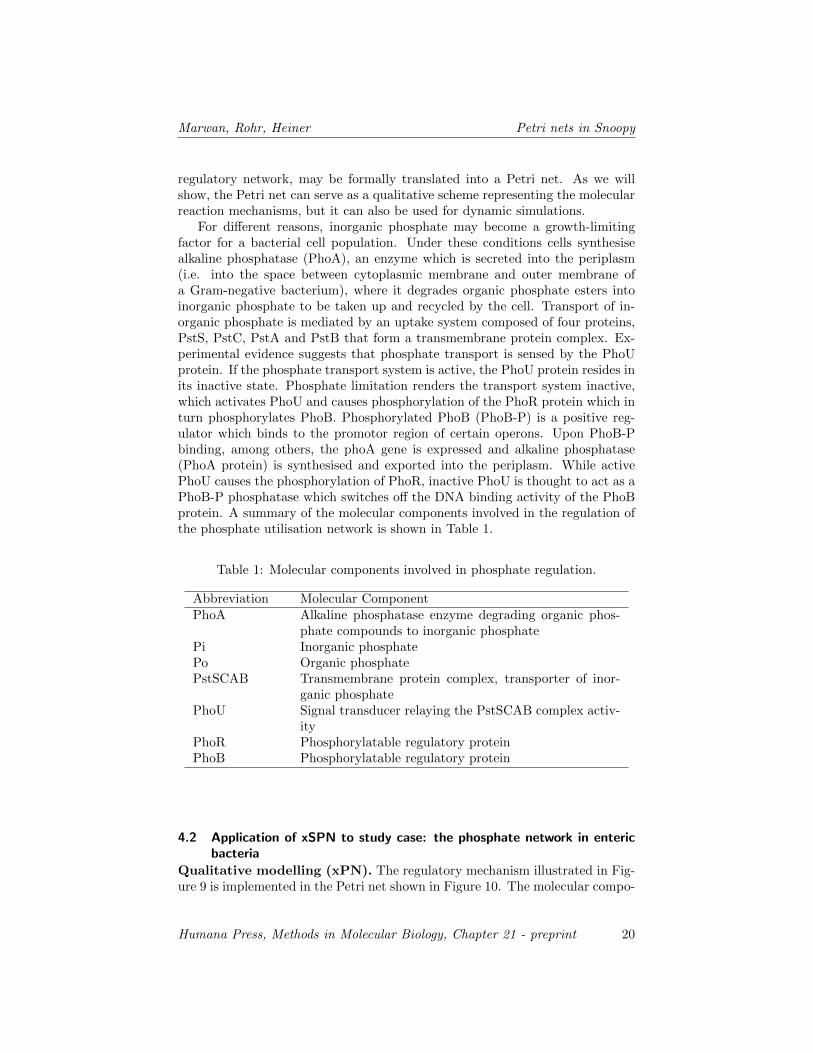
Figure 9: Biochemical model of the phosphate regulatory network in entericbacteria. The scheme is adapted from Neidhardt et al. (1990).

Humana Press, Methods in Molecular Biology, Chapter 21 - preprint 19

Marwan, Rohr, Heiner Petri nets in Snoopy

regulatory network, may be formally translated into a Petri net. As we willshow, the Petri net can serve as a qualitative scheme representing the molecularreaction mechanisms, but it can also be used for dynamic simulations.

For different reasons, inorganic phosphate may become a growth-limitingfactor for a bacterial cell population. Under these conditions cells synthesisealkaline phosphatase (PhoA), an enzyme which is secreted into the periplasm(i.e. into the space between cytoplasmic membrane and outer membrane ofa Gram-negative bacterium), where it degrades organic phosphate esters intoinorganic phosphate to be taken up and recycled by the cell. Transport of in-organic phosphate is mediated by an uptake system composed of four proteins,PstS, PstC, PstA and PstB that form a transmembrane protein complex. Ex-perimental evidence suggests that phosphate transport is sensed by the PhoUprotein. If the phosphate transport system is active, the PhoU protein resides inits inactive state. Phosphate limitation renders the transport system inactive,which activates PhoU and causes phosphorylation of the PhoR protein which inturn phosphorylates PhoB. Phosphorylated PhoB (PhoB-P) is a positive reg-ulator which binds to the promotor region of certain operons. Upon PhoB-Pbinding, among others, the phoA gene is expressed and alkaline phosphatase(PhoA protein) is synthesised and exported into the periplasm. While activePhoU causes the phosphorylation of PhoR, inactive PhoU is thought to act as aPhoB-P phosphatase which switches off the DNA binding activity of the PhoBprotein. A summary of the molecular components involved in the regulation ofthe phosphate utilisation network is shown in Table 1.

Table 1: Molecular components involved in phosphate regulation.

Abbreviation Molecular ComponentPhoA Alkaline phosphatase enzyme degrading organic phos-

phate compounds to inorganic phosphatePi Inorganic phosphatePo Organic phosphatePstSCAB Transmembrane protein complex, transporter of inor-

ganic phosphatePhoU Signal transducer relaying the PstSCAB complex activ-

ityPhoR Phosphorylatable regulatory proteinPhoB Phosphorylatable regulatory protein

4.2 Application of xSPN to study case: the phosphate network in entericbacteria

Qualitative modelling (xPN). The regulatory mechanism illustrated in Fig-ure 9 is implemented in the Petri net shown in Figure 10. The molecular compo-

Humana Press, Methods in Molecular Biology, Chapter 21 - preprint 20

Marwan, Rohr, Heiner Petri nets in Snoopy

nents in their different states (e.g. active, inactive, phosphorylated, unphospho-rylated) are represented as places (Table 2) and their biochemical reactions orfunctional interactions are represented as stochastic transitions (Table 3). Addi-tionally, there are deterministically timed transitions (immediate and scheduledtransitions) to model the experimental addition of inorganic/organic phosphate.There are different arc types. Standard arcs represent the mass flow. Read arcsand inhibitory arcs are used to model regulatory interactions between proteinsthrough physical protein-protein interaction. Double arcs (a sort-hand notationfor two opposite arcs) represent catalytic reactions which may be complex.

The graphical representation of the cytoplasmic membrane and of some pro-teins of interest is put underneath the Petri net in order to explain the modularstructure of the net and to highlight which reactions occur inside or outside thecell, respectively. Note that these graphics are not a functional element of thePetri net as generated in Snoopy. The PstSCAB transmembrane protein com-plex has a dual function as transporter and as a sensor of inorganic phosphate.When inorganic phosphate is present in the periplasm, the PstSCAB complexis phosphorylated through reaction r7. The phosphorylated form, PstSCAB-Pis active in transporting inorganic phosphate through the cytoplasmic mem-brane into the cytoplasm (r5) where it is used for biosynthetic reactions (r6).The PstSCAB protein allosterically controls the activity of the PhoU protein,modelled by read arcs that control the transitions r9 and r10 representing the

Table 2: Petri net places represent molecular components in their differentstates.

Place Molecular componentPi PeriPlasm Inorganic phosphate in the periplasmPi Cytoplasm Inorganic phosphate in the cytoplasmPo PeriPlasm Organic phosphate in the periplasmPhoA Periplasm PhoA protein in the periplasmPhoA PhoA protein in the cytoplasmPhoA mRNA PhoA gene mRNAPstSCAB Transporter of inorganic phosphate, inactive formPstSCAB-P Transporter of inorganic phosphate, phosphorylated, ac-

tive formPhoU inactive Signal transducer, inactive formPhoU active Signal transducer, active formPhoR PhoR protein, dephosphorylated formPhoR-P PhoR protein, phosphorylated formPhoB PhoB protein, dephosphorylated formPhoB-P PhoB protein, phosphorylated formswitch on,switch off

Auxiliary places to model the experiments

Humana Press, Methods in Molecular Biology, Chapter 21 - preprint 21

Marwan, Rohr, Heiner Petri nets in Snoopy

Table 3: Petri net transitions represent biochemical reactions or functional in-teractions. The transitions are stochastic if not specified otherwise.

Transition Reaction or Processr1 Experimental addition of inorganic phosphate (immediate

transition)r2a, r2b Switch on/off the experimental addition by r1 (scheduled

transitions)r3 Environmental source of organic phosphate (immediate

transition)r4 Degradation of organic phosphater5 Transport of inorganic phosphate into the cytoplasmr6 Consumption of inorganic phosphate by biosynthesesr7 Phosphorylation of PstSCAB complexr8 Dephosphorylation of PstSCAB complexr9 Activation of PhoU by PstSCAB complexr10 Deactivation of PhoU by PstSCAB-P complexr11 Phosphorylation of PhoR by active PhoUr12 Phosphorylation of PhoB by PhoR-P, involving dephospho-

rylation of PhoR-Pr13 Dephosphorylation of PhoB-P by inactive PhoUr14 Transcription of the phoA gene upon binding of PhoB-P to

its promoterr15 Decay of the phoA mRNAr16 Translation of the phoA mRNA into PhoA proteinr17 Transport of the PhoA protein into the cytoplasmr18 Denaturation and decay of the periplasmic PhoA protein

activation (r9) and the deactivation (r10) of the PhoU protein, respectively.As long as inorganic phosphate is in the periplasm, the PstSCAB complex iskept in its phosphorylated, transport-active state, modelled by the inhibitoryarc that prevents dephosphorylation via transition r8. In its active form, thePhoU protein causes the phosphorylation of PhoR (r11) which in turn phospho-rylates PhoB. This direct transfer reaction of the phosphate group between thetwo protein molecules is considered as a second order reaction and representedby transition r12. PhoB-P then binds to DNA to promote the transcription ofseveral genes including the phoA gene. The complex process of regulator bind-ing and gene transcription is represented by transition r14. Translation of thephoA mRNA into the PhoA protein occurs through transition r16 which alsosummarizes a complex set of biochemical reactions involving many additionalcomponents. The double arrow linking r16 and the phoA mRNA place indicatesthat from each mRNA molecule many copies of the PhoA protein can be synthe-sized. The PhoA protein is finally transported into the periplasm (r17) where it

Humana Press, Methods in Molecular Biology, Chapter 21 - preprint 22

Marwan, Rohr, Heiner Petri nets in Snoopy

degrades organic phosphate to supply the cell with inorganic phosphate whichin turn switches off the signaling cascade and subsequently the biosynthesis ofthe PhoA protein, as long as sufficient inorganic phosphate enters the cell.

We have already seen how to draw a simple Petri net, so you will not haveany trouble in drawing the Petri net for your first case study. Coarse transitionsand coarse places may be used to structure large networks into modules in orderto improve the readability of the net. Since the Petri net presented for the casestudy is rather small, we did not use coarse nodes here.

Animation of the xPN. To explore the net behaviour, do the followingsteps:

1. load the net (File → Open),

2. start the animation (View → Start Animation Mode),

3. run the net in manual or automatic mode.

Specifically you should check the following scenarios:

1. Which reactions are necessary in which (partial) order to fire the transi-tions Biosynthesis (r6), Decay (r15), or Denaturation&Decay (r18)?

2. Which net behaviour is possible if the inorganic supply is switched on(place switch on is marked), which net behaviour is triggered if the inor-ganic supply is switched off?

3. Try to figure out the maximal token numbers you can get on each place!

4. Is it possible to reach a marking where none of the transitions is enabled?

5. Having played with the net for a while, is it always possible to come backto the given initial marking?

Quantitative modelling (xSPN). All stochastic reactions follow mass-action kinetics with all parameters initially set to 0.1. Afterwards, the parame-ters were adjusted so that the steady state concentration of inorganic phosphatein the periplasm is approximately the same no matter whether the externalsource is inorganic or organic phosphate, respectively: the parameter of r4 isset to 0.2, and the parameter of r15 to 0.075.

The transition t off is scheduled to fire at time point 100, and the transitiont on is scheduled to fire at time point 1000.

Stochastic animation of the xSPN. Follow the stochastic token flow inthe automatic animation mode. Which reaction sequences do you observe whilethe inorganic supply is switched on? What is the difference to the reaction andstate sequences, which you have observed in the animation of the correspondingxPN? The answer lies in the immediate transitions (here r1), which have nowalways highest priority.

Humana Press, Methods in Molecular Biology, Chapter 21 - preprint 23

Marwan, Rohr, Heiner Petri nets in Snoopy

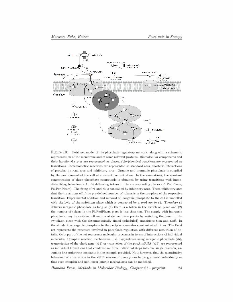
Figure 10: Petri net model of the phosphate regulatory network, along with a schematic

representation of the membrane and of some relevant proteins. Biomolecular components and

their functional states are represented as places, (bio-)chemical reactions are represented as

transitions. Stoichiometric reactions are represented as standard arcs, allosteric interactions

of proteins by read arcs and inhibitory arcs. Organic and inorganic phosphate is supplied

by the environment of the cell at constant concentration. In the simulations, the constant

concentration of these phosphate compounds is obtained by using transitions with imme-

diate firing behaviour (r1, r3) delivering tokens to the corresponding places (Pi PeriPlasm;

Po PeriPlasm). The firing of r1 and r3 is controlled by inhibitory arcs. These inhibitory arcs

shut the transitions off if the pre-defined number of tokens is in the pre-place of the respective

transition. Experimental addition and removal of inorganic phosphate to the cell is modelled

with the help of the switch on place which is connected by a read arc to r1. Therefore r1

delivers inorganic phosphate as long as (1) there is a token in the switch on place and (2)

the number of tokens in the Pi PeriPlasm place is less than ten. The supply with inorganic

phosphate may be switched off and on at defined time points by switching the token in the

switch on place with the deterministically timed (scheduled) transitions t on and t off. In

the simulations, organic phosphate in the periplasm remains constant at all times. The Petri

net represents the processes involved in phosphate regulation with different resolution of de-

tails. Only part of the net represents molecular processes in terms of interactions of individual

molecules. Complex reaction mechanisms, like biosyntheses using inorganic phosphate (r6),

transcription of the phoA gene (r14) or translation of the phoA mRNA (r16) are represented

as individual transitions that condense multiple individual steps into one single reaction, as-

suming first order rate constants in the example provided. Note however, that the quantitative

behaviour of a transition in the xSPN version of Snoopy can be programmed individually so

that even complex and non-linear kinetic mechanisms can be modelled.

Humana Press, Methods in Molecular Biology, Chapter 21 - preprint 24

Marwan, Rohr, Heiner Petri nets in Snoopy

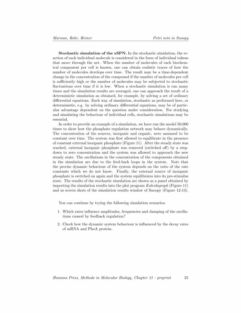
Stochastic simulation of the xSPN. In the stochastic simulation, the re-action of each individual molecule is considered in the form of individual tokensthat move through the net. When the number of molecules of each biochem-ical component per cell is known, one can obtain realistic traces of how thenumber of molecules develops over time. The result may be a time-dependentchange in the concentration of the compound if the number of molecules per cellis sufficiently high or the number of molecules may be subjected to stochasticfluctuations over time if it is low. When a stochastic simulation is run manytimes and the simulation results are averaged, one can approach the result of adeterministic simulation as obtained, for example, by solving a set of ordinarydifferential equations. Each way of simulation, stochastic as performed here, ordeterministic, e.g. by solving ordinary differential equations, may be of partic-ular advantage dependent on the question under consideration. For studyingand simulating the behaviour of individual cells, stochastic simulations may beessential.

In order to provide an example of a simulation, we have run the model 50,000times to show how the phosphate regulation network may behave dynamically.The concentration of the sources, inorganic and organic, were assumed to beconstant over time. The system was first allowed to equilibrate in the presenceof constant external inorganic phosphate (Figure 11). After the steady state wasreached, external inorganic phosphate was removed (switched off) by a step-down to zero concentration and the system was allowed to approach the newsteady state. The oscillations in the concentration of the components obtainedin the simulation are due to the feed-back loops in the system. Note thatthe precise dynamic behaviour of the system depends on the ratio of the rateconstants which we do not know. Finally, the external source of inorganicphosphate is switched on again and the system equilibrates into its pre-stimulusstate. The results of the stochastic simulation are shown as a panel obtained byimporting the simulation results into the plot program Kaleidagraph (Figure 11)and as screen shots of the simulation results window of Snoopy (Figure 12-13).

You can continue by trying the following simulation scenarios:

1. Which rates influence amplitudes, frequencies and damping of the oscilla-tions caused by feedback regulation?

2. Check how the dynamic system behaviour is influenced by the decay ratesof mRNA and PhoA protein.

Humana Press, Methods in Molecular Biology, Chapter 21 - preprint 25

Marwan, Rohr, Heiner Petri nets in Snoopy

0

0.5

1

switch_on

0 500 1000 1500

0

0.5

1

PstSCAB-PPhoU_active

0 500 1000 1500

0

0.5

1

PhoBPhoR-P

0 500 1000 1500

8

9

10

Po_PeriPlasm

0 500 1000 1500

0

0.5

1

PhoB-PphoA mRNAPhoA

0 500 1000 1500

0

4

8

12

16

Pi_PeriPlasmPi_Cytoplasm

0 500 1000 1500

ExternalInorganic Phosphate

ExternalOrganic Phosphate

Num

ber o

f Tok

ens

Time Time

a) b)

c)

d)

e)

f)

Figure 11: Response of the phosphate regulatory network to step-wise changesin the supply of external inorganic phosphate. Traces were obtained by averag-ing 50,000 simulation runs. The rate constants of the stochastic transitions are:r4 0.2, r15 0.075, else 0.1. Initial marking as given in Figure 9. Simulationresults were exported from Snoopy as csv file and imported into Kaleidagraph,see http://www.kaleidagraph.com/, for display.

Humana Press, Methods in Molecular Biology, Chapter 21 - preprint 26

Marwan, Rohr, Heiner Petri nets in Snoopy

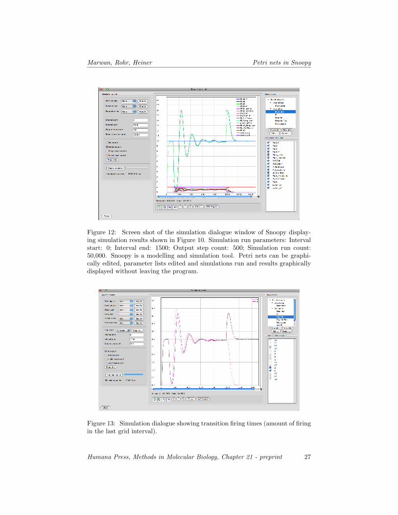
Figure 12: Screen shot of the simulation dialogue window of Snoopy display-ing simulation results shown in Figure 10. Simulation run parameters: Intervalstart: 0; Interval end: 1500; Output step count: 500; Simulation run count:50,000. Snoopy is a modelling and simulation tool. Petri nets can be graphi-cally edited, parameter lists edited and simulations run and results graphicallydisplayed without leaving the program.

Figure 13: Simulation dialogue showing transition firing times (amount of firingin the last grid interval).

Humana Press, Methods in Molecular Biology, Chapter 21 - preprint 27

Marwan, Rohr, Heiner Petri nets in Snoopy

5 Notes1. In this chapter, we deliberately omitted formal definitions. The interested

reader finds them together with accompanying examples of the basic no-tions of biochemically interpreted Petri nets in [4]; for extended Petri netssee specifically [11], for extended stochastic Petri nets [12], and for gen-eral textbooks introducing into Petri nets and stochastic Petri nets thereferences therein.

2. Petri nets represent an inherently concurrent modelling paradigm. Theyallow to distinguish precisely between alternative and concurrent (i.e. in-dependent) behaviour. However for analysis purposes, the partial order(true concurrency) semantics is often reduced to the interleaving seman-tics, where concurrency of reactions is described by all interleaving se-quences of these reactions. We get a state transition system (known inthe Petri net community as reachability graph or marking graph), which isbasically a finite automaton, i.e. a sequential model, and as such does notsupport the differentiation between alternative and concurrent behaviour.This disadvantage is (partially) compensated by the numerous sophisti-cated algorithms and advanced data structures which have been developedfor their efficient analysis.

Nevertheless, often it is advisable to preserve all the concurrency infor-mation, which a biochemical network model enjoys, e.g., to distinguishthe subtle difference between read arcs and two opposite arcs (Figure 7).The partial order semantics yields a behaviour description comprising all(infinite) partial order runs. It is often given as labelled condition/eventnet. Here, transitions represent events, labelled by the name of the reac-tion taking place, while places stand for binary conditions, labelled by thename of the species, set or reset by the event, respectively. Partial orderruns, which can be read as the unfolding of a net structure, give further in-sight into the dynamic behaviour of a network, which may not be apparentfrom the standard net representation. For examples see [4,6], where thebehaviour of subnets induced by T-invariants is given as a partial orderrun.

3. Snoopy supports standard analysis techniques of Petri net theory, such asstatic and dynamic analyses, by export to various analysis tools, see [5].Additionally, Snoopy’s Petri nets are directly read by the Petri net anal-yser Charlie [16]. One of the standard static analysis techniques comprisesthe computation of place and transition invariants, which are often helpfulfor network validation, see e.g. [4,6,17-19], and (Behre et al., this volume).Sets or multi-sets of nodes, such as place and transition invariants, Parikhvectors, structural deadlocks or traps (see [4] for explanations of theseterms), which have been produced with Charlie, are read by Snoopy tovisualize the sub-networks induced by them.

The Petri net of our case study is covered by transition invariants. Thereare five place invariants, and such conservation laws, which are obvi-

Humana Press, Methods in Molecular Biology, Chapter 21 - preprint 28

Marwan, Rohr, Heiner Petri nets in Snoopy

ous in the given case: (switch on, switch off), (PstSCAB, PstSCAB-P),(PhoU inactive, PhoU active), (PhoR, PhoR-P), and (PhoB, PhoB-P).The following five places are not covered by place invariants: Pi PeriPlasm,Po PeriPlasm, Pi CytoPlasm, PhoA Periplasm, PhoA, phoA mRNA; theirmaximal token numbers are determined by the timing constraints.

4. An established analysis technique for special behavioural properties ismodel checking. It checks the Petri net behaviour against propertiesformally specified in temporal logics, see (chapter Batt et al., this vol-ume). Charlie provides some standard explicit model checkers, basicallyfor teaching purposes. Snoopy allows also to export the designed Petrinets to quite a number of model checkers, among them the symbolic modelcheckers BDD-CTL, IDD-CTL [20] and IDD-CSL [21]. Simulation tracesgenerated by Snoopy’s (stochastic or continuous) simulation engines canbe checked againts PLTLc properties with the Monte Carlo Model CheckerMC2 [22]. See [4, 6] for case studies demonstrating a systematic and seam-less model checking approach in the qualitative, stochastic and continuousmodelling paradigms.

5. A given Petri net may also be read as a continuous Petri net, if it isamenable to continuization and the population semantics allows to con-sider just the averaged case. Continuous Petri nets define uniquely a sys-tem of ordinary differential equations (ODEs) [4], but not vice versa. Thepaper [23] demonstrates the structured design of ODEs by the step-wisecomposition of hierarchically structured continuous Petri nets. A familyof related Petri net models builds the core of an integrative approach com-prising qualitative, stochastic and continuous Petri nets, which is demon-strated by a running example each in [4,6]. It also provides an adequateframework to reason about the behavioural relation of models, sharingstructure, but having different kinetics; see, e.g., [24]. For a general out-line of BioModel Engineering see [25].

AcknowledgementsChristian Rohr is funded by the International Max Planck Research Schoolfor Analysis, Design and Optimization in Chemical and Biochemical ProcessEngineering Magdeburg.

References1. Petri, C. A., Reisig, W. (2008) Petri net. Scholarpedia 3(4):6477 http:

//www.scholarpedia.org/article/Petri_net.

2. Marwan, W., Wagler, A., and Weismantel, R. (2009) Petri nets as a frame-work for the reconstruction and analysis of signal transduction pathwaysand regulatory networks. J. Nat. Comput., in press [DOI 10.1007/s11047-009-9152-x].

Humana Press, Methods in Molecular Biology, Chapter 21 - preprint 29

Marwan, Rohr, Heiner Petri nets in Snoopy

3. Baldan, P., Cocco, N., Marin, A. and Simeoni, M. (2010) Petri nets formodelling metabolic pathways: a survey. J. Nat. Comput., in press [DOI10.1007/s11047-010-9180-6].

4. Heiner, M., Gilbert, D., and Donaldson, R. (2008) Petri nets in systemsand synthetic biology. Lect. Notes Comput. Sci.5016: 215-264.

5. Rohr, C., Marwan, W., and Heiner, M. (2010) Snoopy - a unifying Petrinet framework to investigate biomolecular networks; Bioinformatics 26, 7:974-975.

6. Heiner, M., Donaldson, R., and Gilbert, D. (2010) Petri Nets for SystemsBiology. In MS Iyengar (ed.): Symbolic Systems Biology: Theory andMethods, Chapter 3, Jones & Bartlett Publishers, LLC.

7. Petri Nets World: Online Services for the International Petri Nets Com-munity, http://www.informatik.uni-hamburg.de/TGI/PetriNets/.

8. SBML Software Summary: http://sbml.org/SBML_Software_Guide/SBML_Software_Summary.

9. Bitesize Bio Free Online Bioinformatics tools, http://bitesizebio.com/2009/01/06/free-online-bioinformatics-tools/.

10. Systems Biology Software, http://systems-biology.org/software/.

11. Tovchigrechko, A. (2008) Efficient symbolic analysis of bounded Petri netsusing Interval Decision Diagrams; Ph.D. Thesis, BTU Cottbus, Germany.

12. Heiner, M., Lehrack, S., Gilbert, D., and Marwan, W. (2009) ExtendedStochastic Petri Nets for Model-Based Design of Wet-lab Experiments.Lect. Notes Bioinformatics 5750: 138-163.

13. Gillespie, D. T. (1977) Exact stochastic simulation of coupled chemicalreactions; J/ Phys. Chem. 81(25): 2340-2361.

14. Neidhardt, F. C., Ingraham, J. L. et al. (1990). Physiology of the Bac-terial Cell - A Molecular Approach. Sunderland, Massachusetts, SinauerAssociates. p. 370.

15. Yi-Ju Hsieh, Y.-J. and Wanner, B.L. (2010) Global regulation by theseven-component Pi signaling system. Curr. Opin. Microbiol. 13:198-203.

16. Franzke, A. (2009) Charlie 2.0 - a multi-threaded Petri net analyser.Diploma Thesis, BTU Cottbus, Germany.

17. Heiner, M., and Koch, I. (2004) Petri Net Based System Validation inSystems Biology. Lect. Notes Comput. Sci. 3099: 216-237.

Humana Press, Methods in Molecular Biology, Chapter 21 - preprint 30

Marwan, Rohr, Heiner Petri nets in Snoopy

18. Palsson, B.O. (2006) Systems Biology: Properties of Reconstructed Net-works. Cambridge University Press.

19. Heiner, M. (2009) Understanding Network Behaviour by Structured Rep-resentations of Transition Invariants - A Petri Net Perspective on Systemsand Synthetic Biology. In A Condon, D Harel, JN Kok, A Salomaa, EWinfree (eds.) Algorithmic Bioprocesses. Springer, Natural ComputingSeries, 367-389.

20. Heiner, M., Schwarick, M., and Tovchigrechko, A. (2009) DSSZ-MC - ATool for Symbolic Analysis of Extended Petri Nets. Lect. Notes Comput.Sci. 5606: 323-332.

21. Schwarick, M., and Heiner, M. (2009) CSL model checking of biochemicalnetworks with Interval Decision Diagrams. Lect. Notes Bioinformatics5688: 296-312.

22. MC2(PLTLc) - Monte Carlo Model Checker for PLTLc properties, Uni-versity of Glasgow, http://www.brc.dcs.gla.ac.uk/software/mc2/.

23. Breitling, R., Gilbert, D., Heiner, M., and Orton, R. (2008) A structuredapproach for the engineering of biochemical network models, illustratedfor signalling pathways. Brief. Bioinformatics 9: 404-421.

24. Heiner, M., and Sriram, K. (2010) Structural Analysis to Determine theCore of Hypoxia Response Network. PLoS ONE 5(1): e8600.

25. Breitling, R.; Donaldson, R.A.; Gilbert, D.; Heiner, M. (2010) BiomodelEngineering - From Structure to Behavior. Lect. Notes Bioinformatics5945, 1-12.

Humana Press, Methods in Molecular Biology, Chapter 21 - preprint 31