Pertemuan 15 - 16 CLOSED CONDUIT FLOW 2. Types of Engineering Problems How big does the pipe have to be to carry a flow of x m 3 /s? How big does the.

Pertemuan 15 - 16Pertemuan 15 - 16CLOSED CONDUIT FLOW 2CLOSED CONDUIT FLOW 2

Types of Engineering Types of Engineering ProblemsProblems

• How big does the pipe have to be to How big does the pipe have to be to carry a flow of x mcarry a flow of x m33/s?/s?

• What will the pressure in the water What will the pressure in the water distribution system be when a fire distribution system be when a fire hydrant is open?hydrant is open?

• Can we increase the flow in this old Can we increase the flow in this old pipe by adding a smooth liner?pipe by adding a smooth liner?

Viscous Flow in Pipes: Viscous Flow in Pipes: OverviewOverview

• Boundary Layer DevelopmentBoundary Layer Development

• TurbulenceTurbulence

• Velocity DistributionsVelocity Distributions

• Energy LossesEnergy Losses– MajorMajor– MinorMinor

• Solution TechniquesSolution Techniques

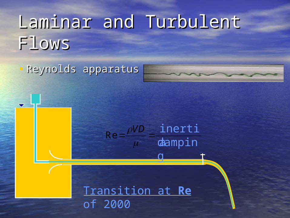
Transition at Re of 2000

Laminar and Turbulent Laminar and Turbulent FlowsFlows• Reynolds apparatusReynolds apparatus

ReVD

dampinginertia

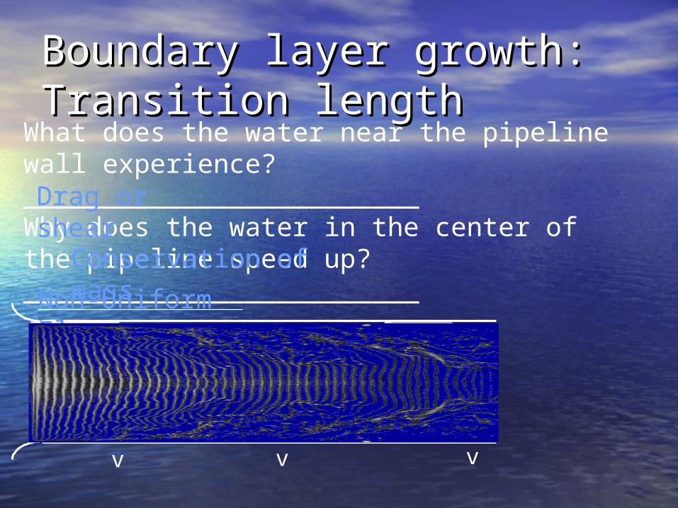
Boundary layer growth: Boundary layer growth: Transition lengthTransition length

What does the water near the pipeline wall experience? _________________________Why does the water in the center of the pipeline speed up? _________________________

v v

Drag or shear

Conservation of mass

Non-Uniform Flow

v

Entrance Region LengthEntrance Region Length

1

10

100

Re

l e /D

1/ 64.4 Reel

D0.06Reel

D

laminar turbulent

Reel fD

Distance for velocity profile to develop

Shear in the entrance region vs shear in long pipes?

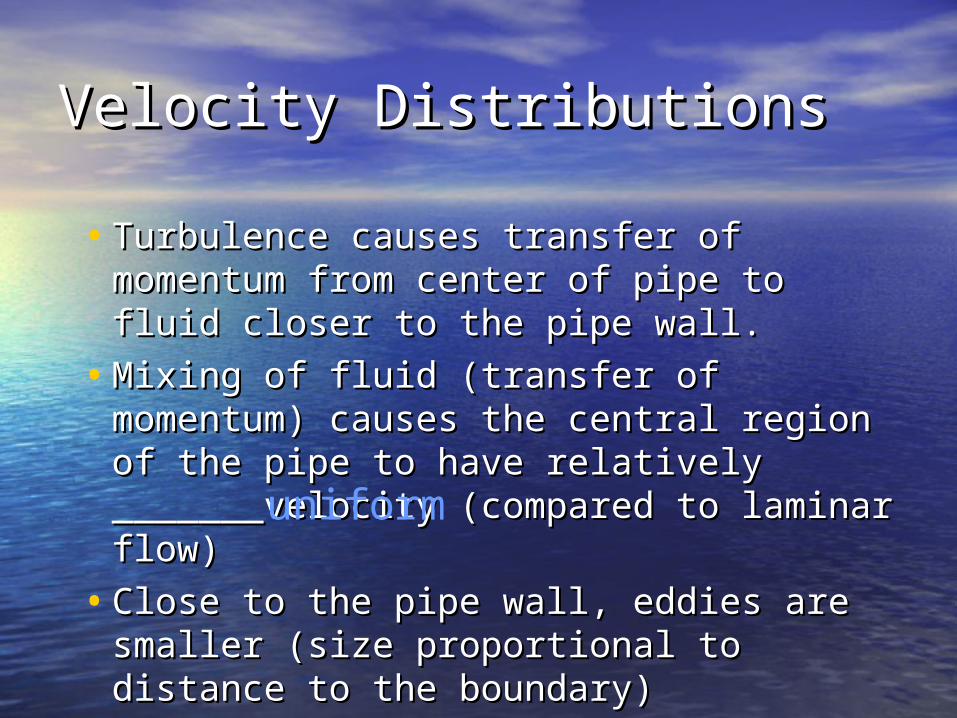
Velocity DistributionsVelocity Distributions

• Turbulence causes transfer of Turbulence causes transfer of momentum from center of pipe to fluid momentum from center of pipe to fluid closer to the pipe wall.closer to the pipe wall.

• Mixing of fluid (transfer of momentum) Mixing of fluid (transfer of momentum) causes the central region of the pipe to causes the central region of the pipe to have relatively _______velocity have relatively _______velocity (compared to laminar flow)(compared to laminar flow)

• Close to the pipe wall, eddies are Close to the pipe wall, eddies are smaller (size proportional to distance smaller (size proportional to distance to the boundary)to the boundary)

uniform

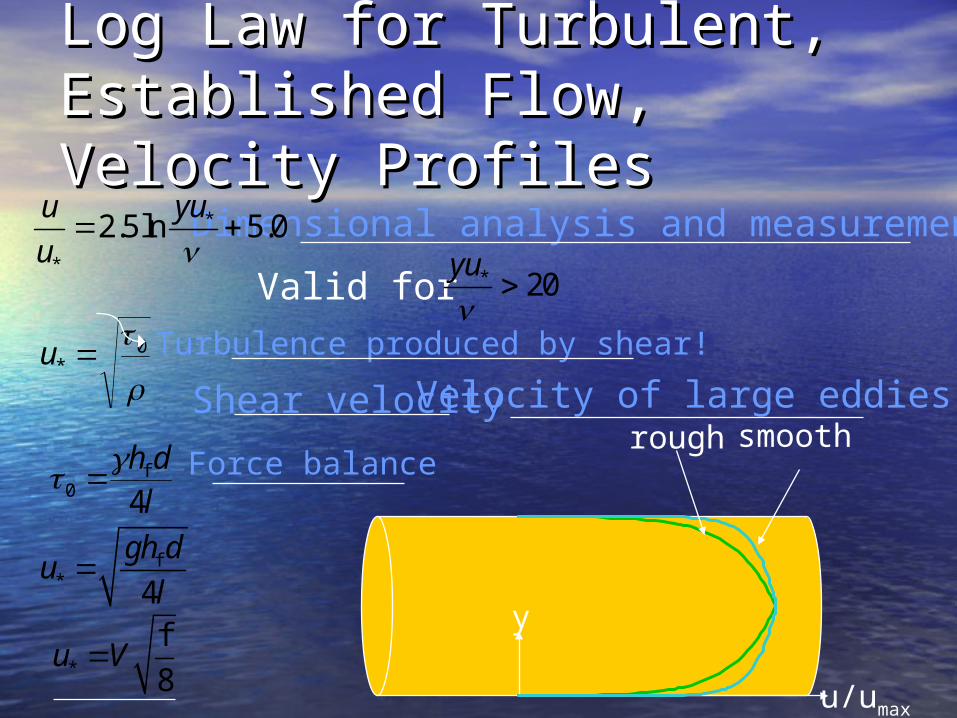
Shear velocity

Dimensional analysis and measurements

Velocity of large eddies

Log Law for Turbulent, Log Law for Turbulent, Established Flow, Velocity Established Flow, Velocity ProfilesProfiles

*

*

2.5ln 5.0yuu

u

0* u

u/umax

rough smooth

y

f0 4

h d

l

f* 4

gh du

l

Force balance

Turbulence produced by shear!

*

f

8u V

Valid for * 20yu

Pipe Flow: The ProblemPipe Flow: The Problem

• We have the control volume energy We have the control volume energy equation for pipe flowequation for pipe flow

• We need to be able to predict the We need to be able to predict the head loss term.head loss term.

• We will use the results we obtained We will use the results we obtained using dimensional analysisusing dimensional analysis

Viscous Flow: Dimensional Viscous Flow: Dimensional AnalysisAnalysis

in a bounded region (pipes, rivers): find Cp

flow around an immersed object : find Cd

• Remember dimensional analysis?Remember dimensional analysis?

• Two important parameters!Two important parameters!– Re - Laminar or TurbulentRe - Laminar or Turbulent– /D - Rough or Smooth/D - Rough or Smooth

• Flow geometryFlow geometry– internal _______________________________internal _______________________________– external _______________________________external _______________________________

,Rep

DC f

l D

2

2C

Vp

p Re

VD

Where and

Dimensional Analysis

Darcy-Weisbach equation

Pipe Flow Energy LossesPipe Flow Energy Losses

f ,Rep

DC f

L D

2

2C

Vp

p

2

2C

V

ghlp

f2

2f

gh D

V L

2

f f2

L Vh

D g

lgh p

Always true (laminar or turbulent)

Assume horizontal flow

More general

lgh p g z

2*2

f=8u

V

2*

f 82

uLh

D g

Friction Factor : Major lossesFriction Factor : Major losses

• Laminar flowLaminar flow

• Turbulent (Smooth, Transition, Turbulent (Smooth, Transition, Rough) Rough)

• Colebrook FormulaColebrook Formula

• Moody diagramMoody diagram

• Swamee-JainSwamee-Jain

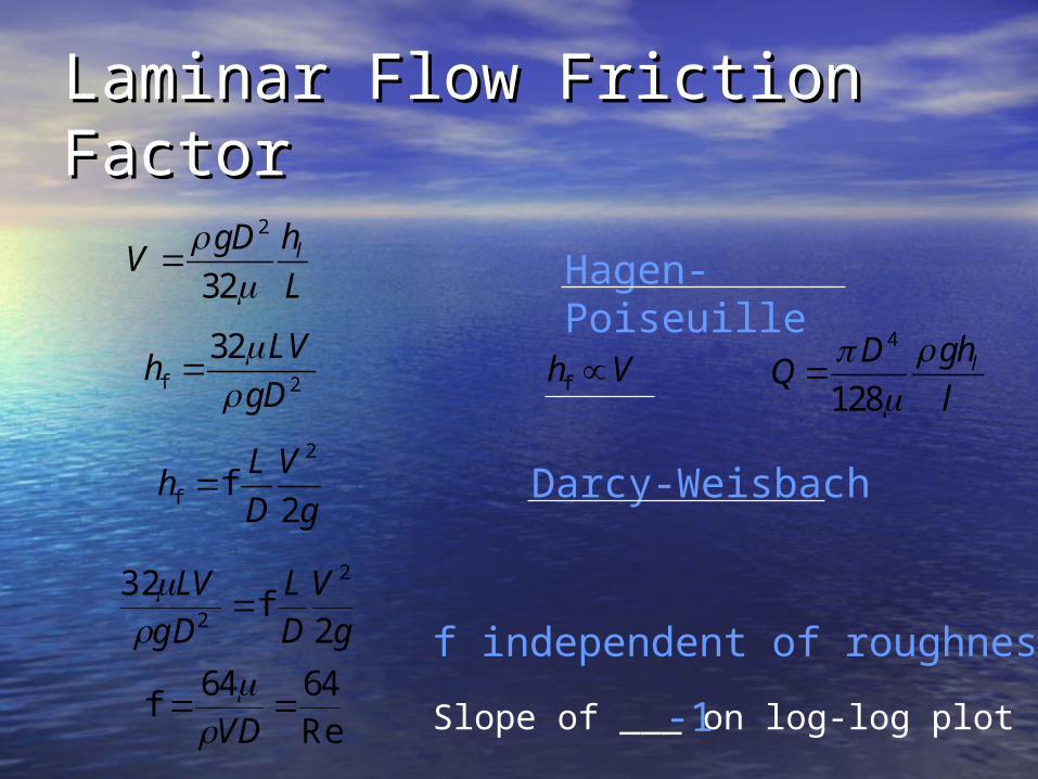
Hagen-Poiseuille

Darcy-Weisbach

Laminar Flow Friction FactorLaminar Flow Friction Factor

2

32lhgD

VL

f 2

32 LVh

gD

2

f f2

L Vh

D g

gV

DL

gDLV

2f

32 2

2

64 64f

ReVD

Slope of ___ on log-log plot-1

fh V

f independent of roughness!

4

128lghD

Ql

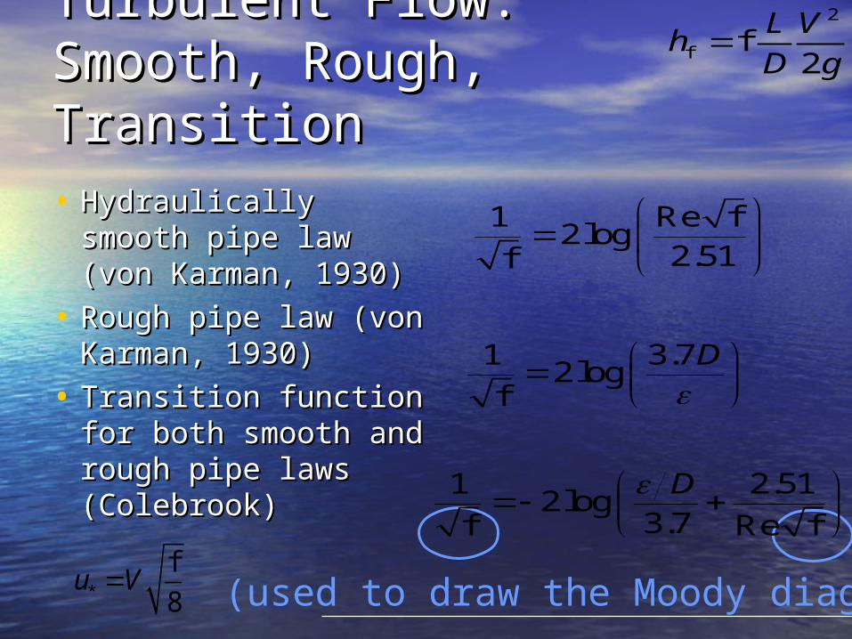
Turbulent Flow:Turbulent Flow:Smooth, Rough, Transition Smooth, Rough, Transition • Hydraulically Hydraulically

smooth pipe law smooth pipe law (von Karman, 1930)(von Karman, 1930)

• Rough pipe law (von Rough pipe law (von Karman, 1930)Karman, 1930)

• Transition function Transition function for both smooth and for both smooth and rough pipe laws rough pipe laws (Colebrook)(Colebrook)

1 Re f2log

2.51f

1 3.72log

f

D

2

f f2

L Vh

D g

(used to draw the Moody diagram)

1 2.512log

3.7f Re f

D

*

f

8u V

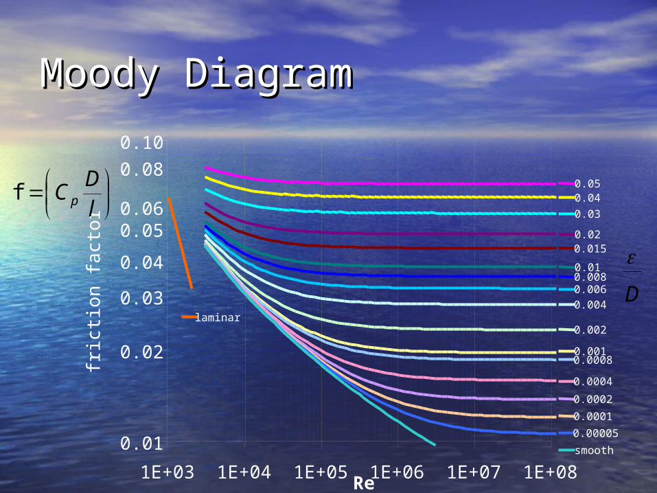
Moody DiagramMoody Diagram

0.01

0.10

1E+03 1E+04 1E+05 1E+06 1E+07 1E+08Re

fric

tion

fact

or

laminar

0.050.04

0.03

0.020.015

0.010.0080.006

0.004

0.002

0.0010.0008

0.0004

0.0002

0.0001

0.00005

smooth

lD

C pf

D

0.02

0.03

0.04

0.050.06

0.08

Swamee-JainSwamee-Jain• 19761976

• limitationslimitations– /D < 2 x 10/D < 2 x 10-2-2

– Re >3 x 10Re >3 x 1033

– less than 3% less than 3% deviation from deviation from results obtained results obtained with Moody diagramwith Moody diagram

• easy to program easy to program for computer or for computer or calculator usecalculator use

0.044.75 5.221.25 9.4

f f

0.66LQ L

D Qgh gh

2

0.9

0.25f

5.74log

3.7 ReD

no f

Each equation has two terms. Why?

5/ 2 f3

f

log 2.513.7 22

gh LQ D

L D gh D

Colebrook

Pipe roughnessPipe roughnesspipe material pipe roughness (mm)

glass, drawn brass, copper 0.0015

commercial steel or wrought iron 0.045

asphalted cast iron 0.12

galvanized iron 0.15

cast iron 0.26

concrete 0.18-0.6

rivet steel 0.9-9.0

corrugated metal 45PVC 0.12

d Must be

dimensionless!

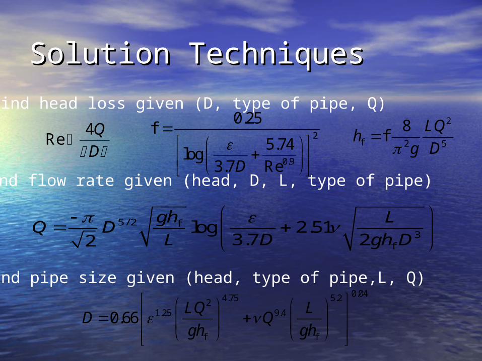
find head loss given (D, type of pipe, Q)

find flow rate given (head, D, L, type of pipe)

find pipe size given (head, type of pipe,L, Q)

Solution TechniquesSolution Techniques

0.044.75 5.221.25 9.4

f f

0.66LQ L

D Qgh gh

2

f 2 5

8f

LQh

g D2

0.9

0.25f

5.74log

3.7 ReD

Re 4QD

5/ 2 f3

f

log 2.513.7 22

gh LQ D

L D gh D

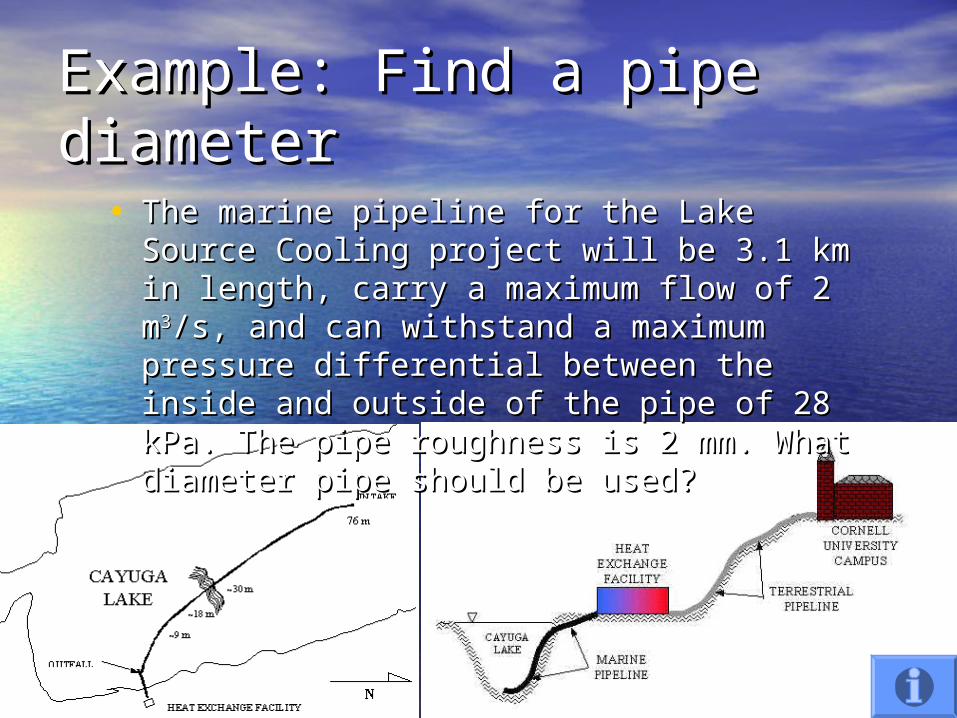
Example: Find a pipe Example: Find a pipe diameterdiameter

• The marine pipeline for the Lake Source The marine pipeline for the Lake Source Cooling project will be 3.1 km in length, Cooling project will be 3.1 km in length, carry a maximum flow of 2 mcarry a maximum flow of 2 m33/s, and can /s, and can withstand a maximum pressure differential withstand a maximum pressure differential between the inside and outside of the pipe between the inside and outside of the pipe of 28 kPa. The pipe roughness is 2 mm. of 28 kPa. The pipe roughness is 2 mm. What diameter pipe should be used?What diameter pipe should be used?

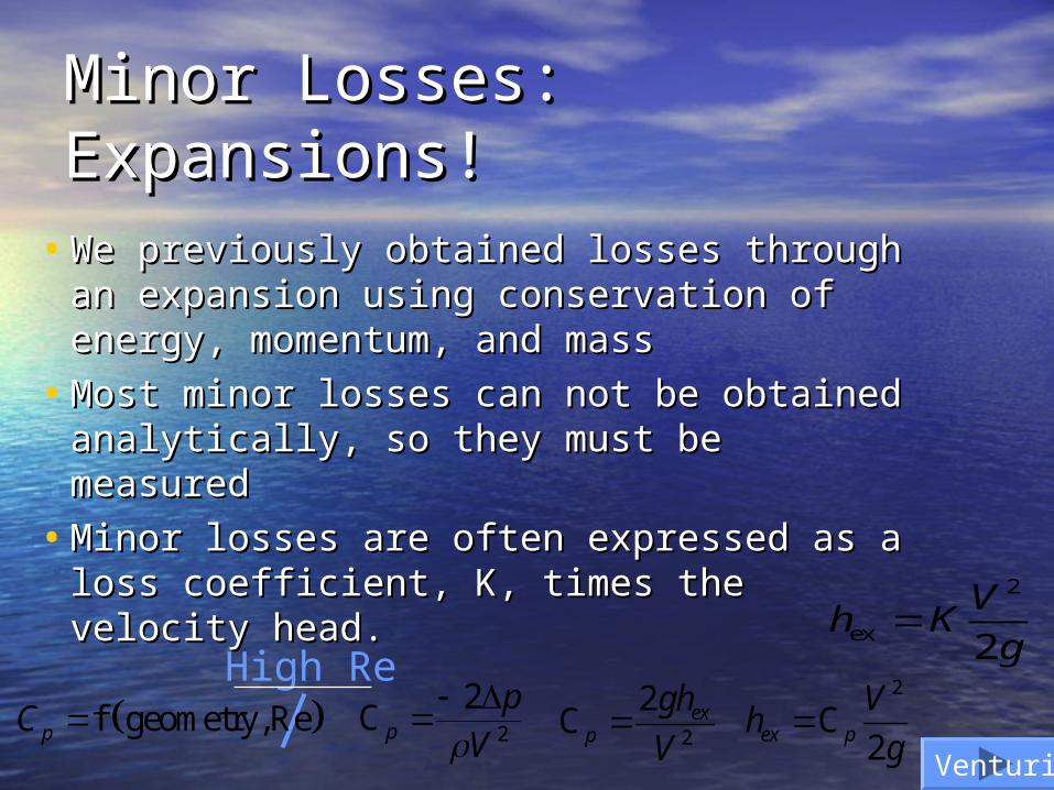
Minor Losses: Expansions!Minor Losses: Expansions!

• We previously obtained losses through We previously obtained losses through an expansion using conservation of an expansion using conservation of energy, momentum, and massenergy, momentum, and mass

• Most minor losses can not be obtained Most minor losses can not be obtained analytically, so they must be measuredanalytically, so they must be measured

• Minor losses are often expressed as a Minor losses are often expressed as a loss coefficient, K, times the velocity loss coefficient, K, times the velocity head.head.

2

ex 2

Vh K

g

f geometry,RepC 2

2C

Vp

p

2

2C ex

p

gh

V

2

C2ex p

Vh

g

Venturi

High Re

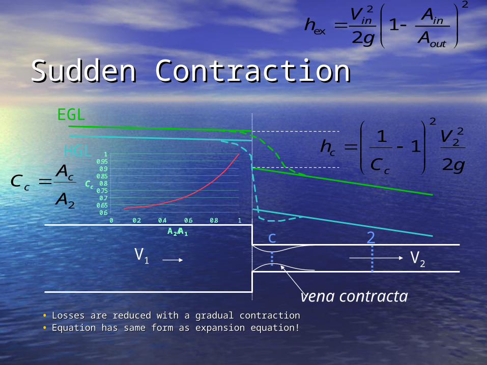
Sudden ContractionSudden Contraction

V1 V2

EGL

HGL

vena contracta• Losses are reduced with a gradual contractionLosses are reduced with a gradual contraction• Equation has same form as expansion equation!Equation has same form as expansion equation!

g

V

Ch

c

c

21

1 22

2

2A

AC c

c

0.60.650.7

0.750.8

0.850.9

0.951

0 0.2 0.4 0.6 0.8 1

A2/A1

Cc

0.60.650.7

0.750.8

0.850.9

0.951

0 0.2 0.4 0.6 0.8 1

A2/A1

Cc

0.60.650.7

0.750.8

0.850.9

0.951

0 0.2 0.4 0.6 0.8 1

A2/A1

Cc

c 2

22

ex 12

in in

out

V Ah

g A

g

VKh ee

2

2

0.1eK

5.0eK

04.0eK

Entrance LossesEntrance Losses

Losses can be Losses can be reduced by reduced by accelerating the accelerating the flow gradually and flow gradually and eliminating theeliminating the

vena contracta

Estimate based on contraction equations!

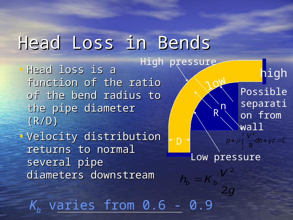
Head Loss in BendsHead Loss in Bends• Head loss is a function Head loss is a function

of the ratio of the of the ratio of the bend radius to the bend radius to the pipe diameter (R/D)pipe diameter (R/D)

• Velocity distribution Velocity distribution returns to normal returns to normal several pipe several pipe diameters diameters downstreamdownstream

High pressure

Low pressure

Possible separation from wall

D

R

g

VKh bb

2

2

Kb varies from 0.6 - 0.9

2Vp dn z C

R

n

lowhigh

Head Loss in ValvesHead Loss in Valves

• Function of valve type and Function of valve type and valve positionvalve position

• The complex flow path The complex flow path through valves can result through valves can result in high head loss (of in high head loss (of course, one of the course, one of the purposes of a valve is to purposes of a valve is to create head loss when it is create head loss when it is not fully open)not fully open)

g

VKh vv

2

2

Can Kvbe greater than 1? ______

2

2 4

8v v

Qh K

g D

What is V?

Yes!

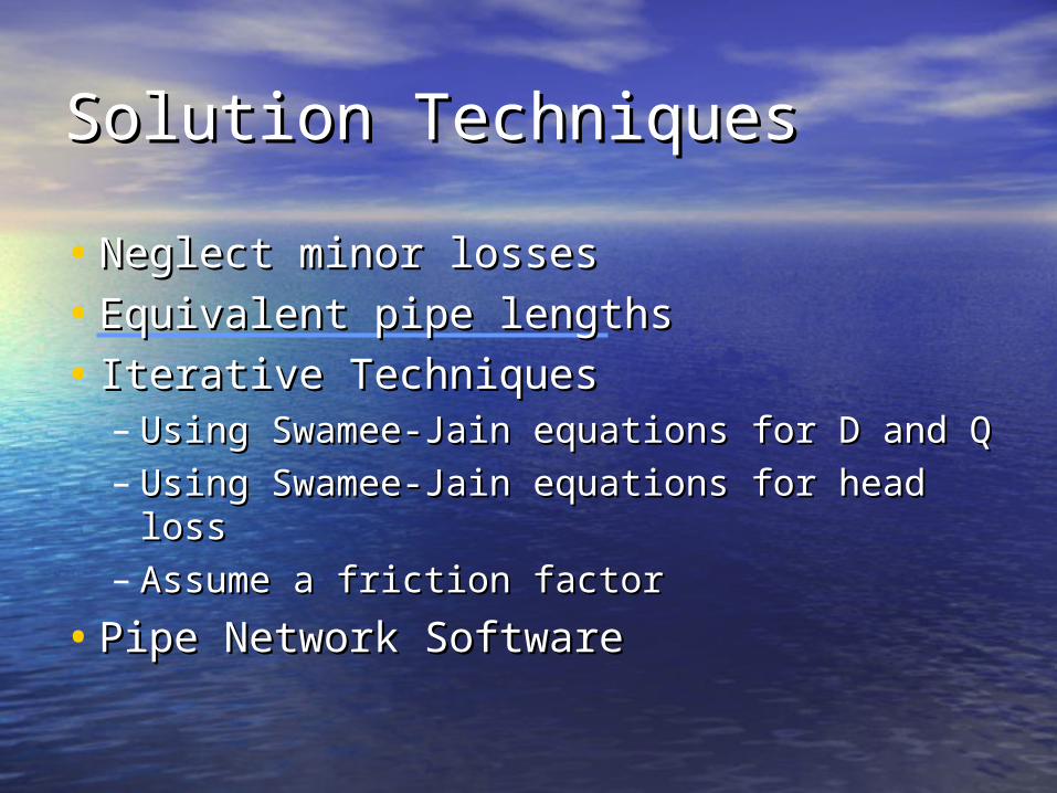
Solution TechniquesSolution Techniques

• Neglect minor lossesNeglect minor losses

• Equivalent pipe lengthsEquivalent pipe lengths

• Iterative TechniquesIterative Techniques– Using Swamee-Jain equations for D and QUsing Swamee-Jain equations for D and Q– Using Swamee-Jain equations for head lossUsing Swamee-Jain equations for head loss– Assume a friction factorAssume a friction factor

• Pipe Network SoftwarePipe Network Software

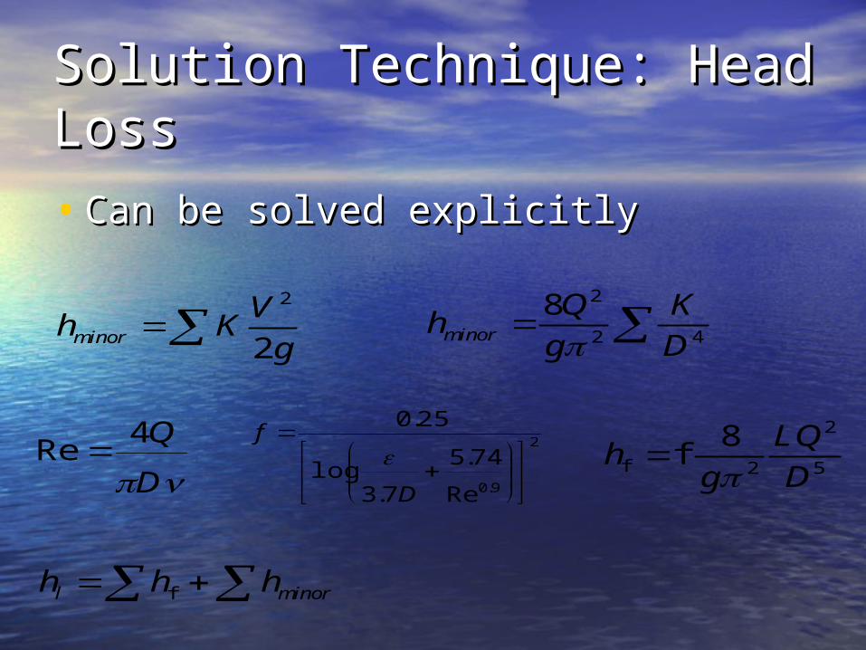
Solution Technique: Head Solution Technique: Head LossLoss

• Can be solved explicitlyCan be solved explicitly

fl minorh h h

2

2minor

Vh K

g

2

f 2 5

8f

LQh

g D2

9.0Re

74.5

7.3log

25.0

D

f

2

2 4

8minor

Q Kh

g D

D

Q4Re

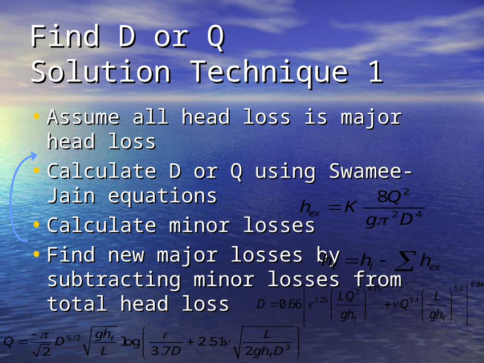
Find D or Q Find D or Q Solution Technique 1Solution Technique 1

• Assume all head loss is major head Assume all head loss is major head lossloss

• Calculate D or Q using Swamee-Jain Calculate D or Q using Swamee-Jain equationsequations

• Calculate minor lossesCalculate minor losses

• Find new major losses by subtracting Find new major losses by subtracting minor losses from total head loss minor losses from total head loss 0.044.75 5.22

1.25 9.4

f f

0.66LQ L

D Qgh gh

2

2 4

8ex

Qh K

g D

f l exh h h

5/ 2 f3

f

log 2.513.7 22

gh LQ D

L D gh D

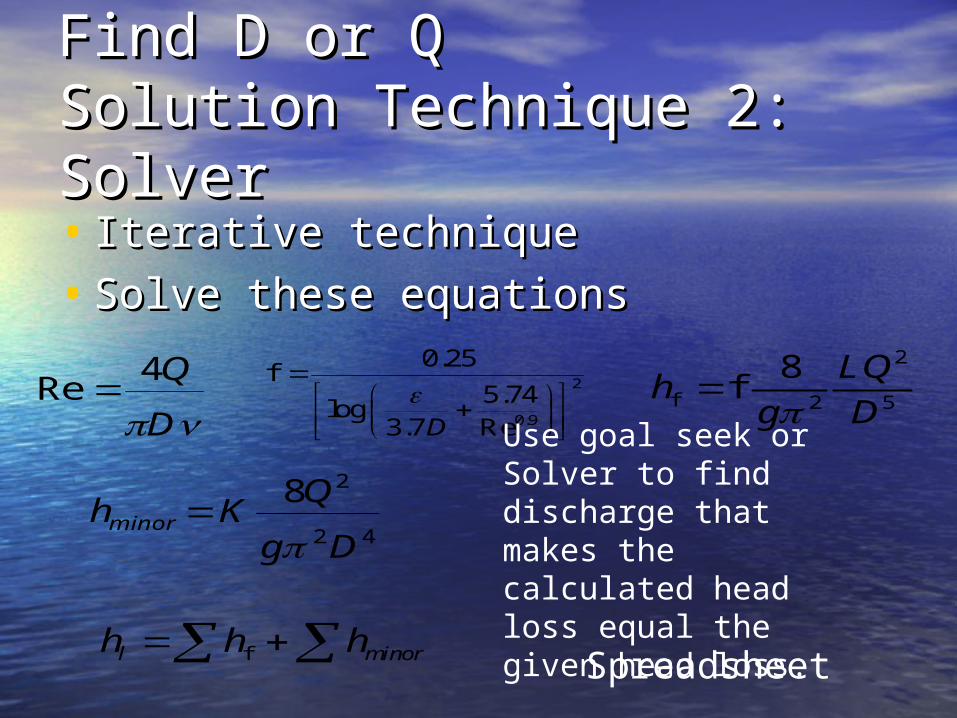
Find D or Q Find D or Q Solution Technique 2: Solver Solution Technique 2: Solver

• Iterative techniqueIterative technique

• Solve these equationsSolve these equations

fl minorh h h

42

28

Dg

QKhminor

2

f 2 5

8f

LQh

g D2

0.9

0.25f

5.74log

3.7 ReD

D

Q4Re

Use goal seek or Solver to find discharge that makes the calculated head loss equal the given head loss.

Spreadsheet

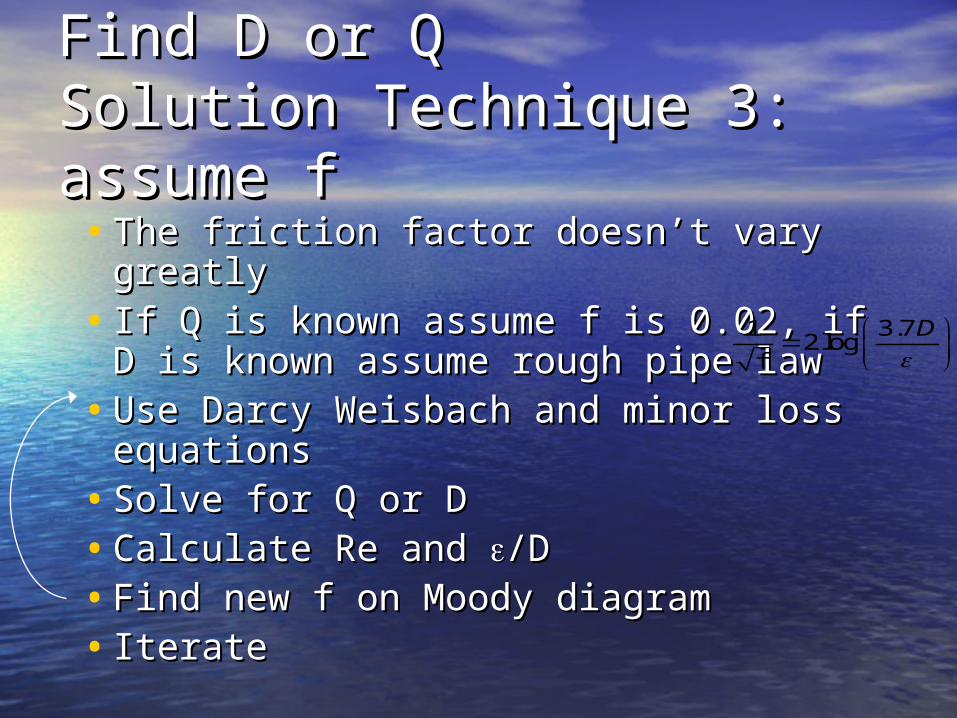
Find D or QFind D or QSolution Technique 3: Solution Technique 3: assume fassume f• The friction factor doesn’t vary The friction factor doesn’t vary

greatlygreatly• If Q is known assume f is 0.02, if D is If Q is known assume f is 0.02, if D is

known assume rough pipe lawknown assume rough pipe law• Use Darcy Weisbach and minor loss Use Darcy Weisbach and minor loss

equationsequations• Solve for Q or DSolve for Q or D• Calculate Re and Calculate Re and /D/D• Find new f on Moody diagramFind new f on Moody diagram• Iterate Iterate

1 3.72log

f

D

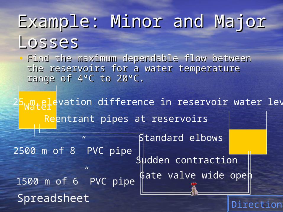
Example: Minor and Major Example: Minor and Major LossesLosses• Find the maximum dependable flow between the Find the maximum dependable flow between the

reservoirs for a water temperature range of 4ºC to reservoirs for a water temperature range of 4ºC to 20ºC. 20ºC.

Water

2500 m of 8” PVC pipe

1500 m of 6” PVC pipeGate valve wide open

Standard elbows

Reentrant pipes at reservoirs

25 m elevation difference in reservoir water levels

Sudden contraction

DirectionsSpreadsheet

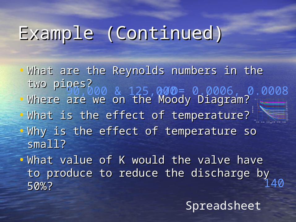
Example (Continued)Example (Continued)

• What are the Reynolds numbers in the What are the Reynolds numbers in the two pipes?two pipes?

• Where are we on the Moody Diagram?Where are we on the Moody Diagram?

• What is the effect of temperature?What is the effect of temperature?

• Why is the effect of temperature so Why is the effect of temperature so small?small?

• What value of K would the valve have to What value of K would the valve have to produce to reduce the discharge by 50%?produce to reduce the discharge by 50%?

0.01

0.1

1E+03 1E+04 1E+05 1E+06 1E+07 1E+08Re

fric

tion

fact

or

laminar

0.050.04

0.03

0.020.015

0.010.0080.006

0.004

0.002

0.0010.0008

0.0004

0.0002

0.0001

0.00005

smooth

90,000 & 125,000

140

/D= 0.0006, 0.0008

Spreadsheet

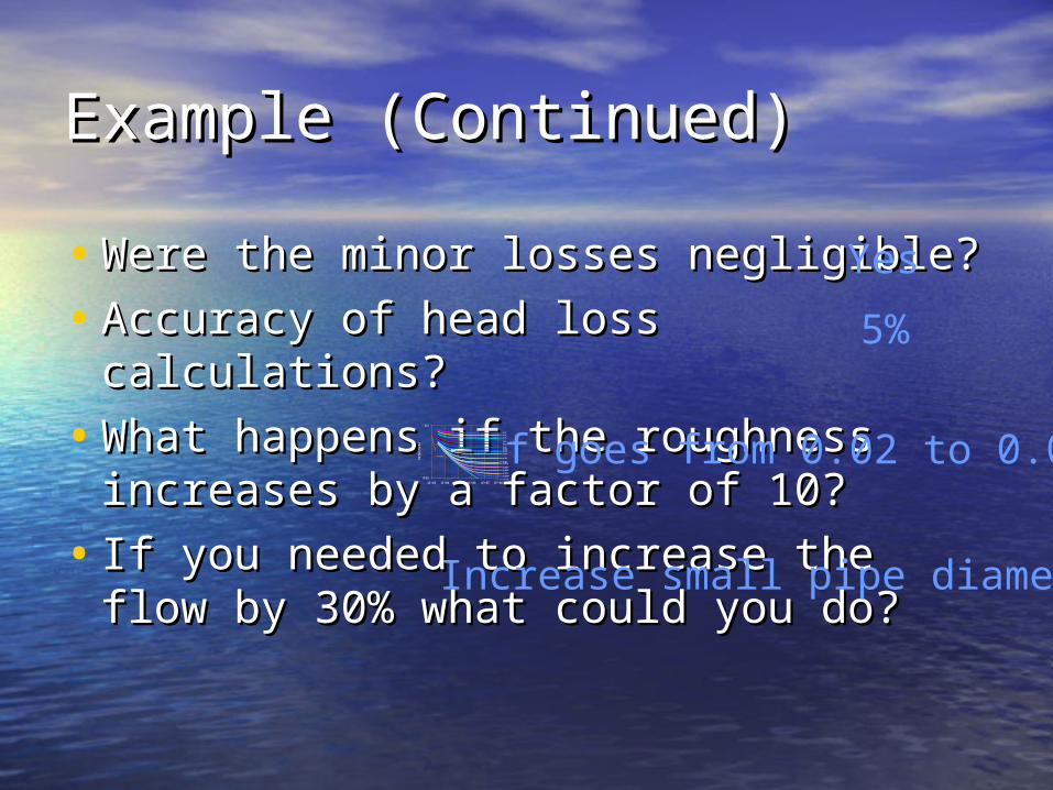
Example (Continued)Example (Continued)

• Were the minor losses negligible?Were the minor losses negligible?

• Accuracy of head loss calculations?Accuracy of head loss calculations?

• What happens if the roughness What happens if the roughness increases by a factor of 10?increases by a factor of 10?

• If you needed to increase the flow by If you needed to increase the flow by 30% what could you do?30% what could you do?

0.01

0.1

1E+03 1E+04 1E+05 1E+06 1E+07 1E+08Re

fric

tion

fact

or

laminar

0.050.04

0.03

0.020.015

0.010.0080.006

0.004

0.002

0.0010.0008

0.0004

0.0002

0.0001

0.00005

smooth

Yes

5%

f goes from 0.02 to 0.035

Increase small pipe diameter

Pipe Flow Summary (1)Pipe Flow Summary (1)

linearly

experimental

• Shear increases _________ with Shear increases _________ with distance from the center of the pipe distance from the center of the pipe (for both laminar and turbulent flow)(for both laminar and turbulent flow)

• Laminar flow losses and velocity Laminar flow losses and velocity distributions can be derived based on distributions can be derived based on momentum (Navier Stokes) and momentum (Navier Stokes) and energy conservationenergy conservation

• Turbulent flow losses and velocity Turbulent flow losses and velocity distributions require ___________ distributions require ___________ resultsresults

Pipe Flow Summary (2)Pipe Flow Summary (2)

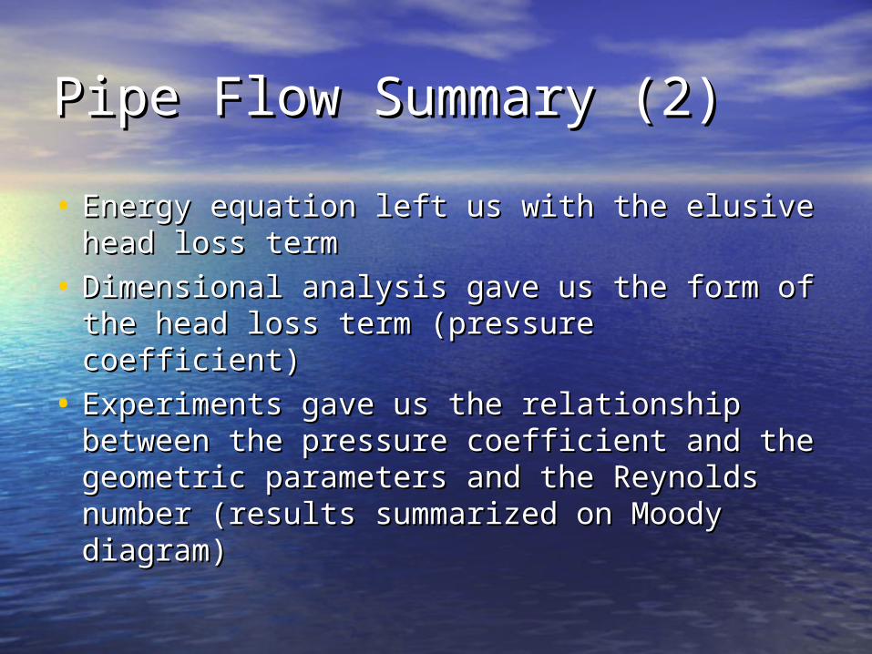
• Energy equation left us with the elusive Energy equation left us with the elusive head loss termhead loss term

• Dimensional analysis gave us the form of Dimensional analysis gave us the form of the head loss term (pressure coefficient)the head loss term (pressure coefficient)

• Experiments gave us the relationship Experiments gave us the relationship between the pressure coefficient and the between the pressure coefficient and the geometric parameters and the Reynolds geometric parameters and the Reynolds number (results summarized on Moody number (results summarized on Moody diagram)diagram)

Pipe Flow Summary (3)Pipe Flow Summary (3)

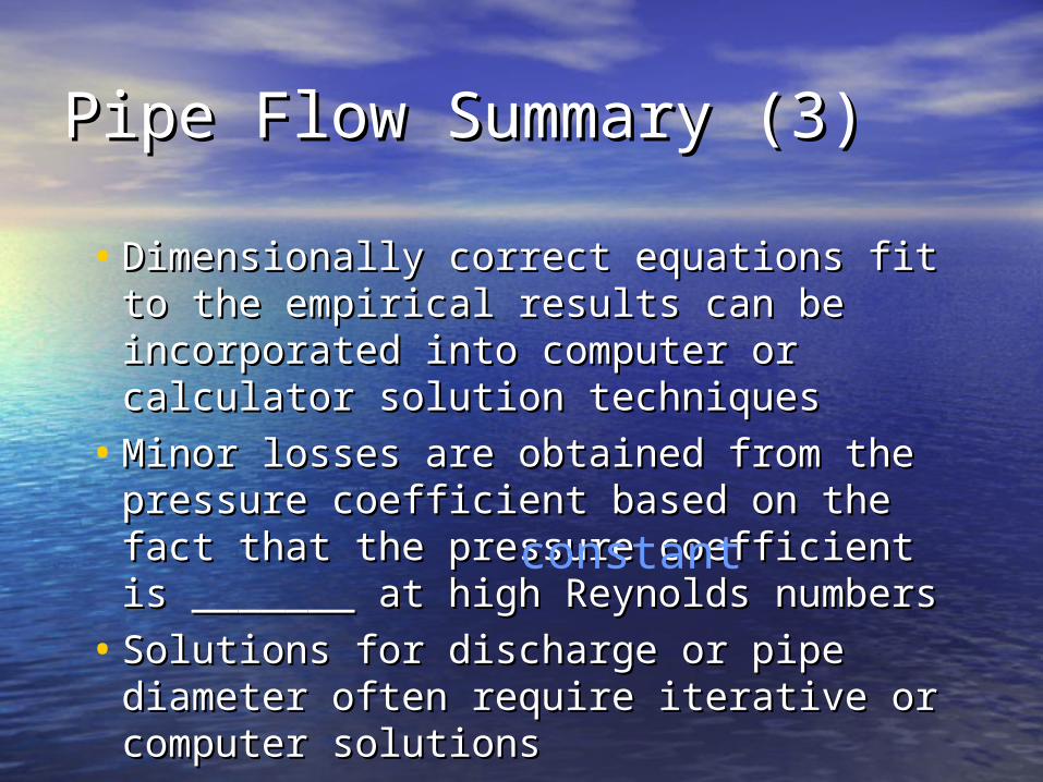
• Dimensionally correct equations fit to Dimensionally correct equations fit to the empirical results can be the empirical results can be incorporated into computer or incorporated into computer or calculator solution techniquescalculator solution techniques

• Minor losses are obtained from the Minor losses are obtained from the pressure coefficient based on the fact pressure coefficient based on the fact that the pressure coefficient is _______ that the pressure coefficient is _______ at high Reynolds numbersat high Reynolds numbers

• Solutions for discharge or pipe Solutions for discharge or pipe diameter often require iterative or diameter often require iterative or computer solutionscomputer solutions

constant

Pressure Coefficient for a Pressure Coefficient for a Venturi MeterVenturi Meter

1

10

1E+00 1E+01 1E+02 1E+03 1E+04 1E+05 1E+06

Re

Cp

ReVl

2

2C

Vp

p

0.01

0.1

1E+03 1E+04 1E+05 1E+06 1E+07 1E+08Re

fric

tion

fact

or

laminar

0.050.04

0.03

0.020.015

0.010.0080.006

0.004

0.002

0.0010.0008

0.0004

0.0002

0.0001

0.00005

smooth

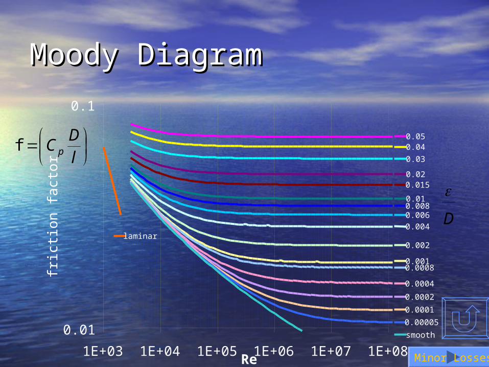
Moody DiagramMoody Diagram

0.01

0.1

1E+03 1E+04 1E+05 1E+06 1E+07 1E+08Re

fric

tion

fact

or

laminar

0.050.04

0.03

0.020.015

0.010.0080.006

0.004

0.002

0.0010.0008

0.0004

0.0002

0.0001

0.00005

smooth

lD

C pf

D

Minor Losses

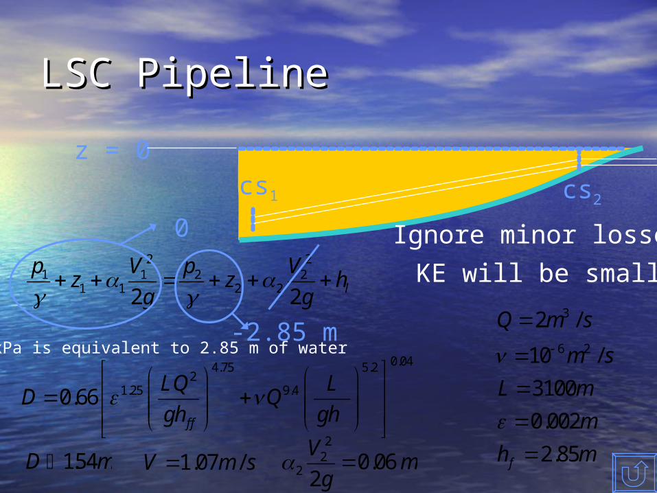
LSC PipelineLSC Pipeline

cs1 cs2

2 21 1 2 2

1 1 2 22 2 l

p V p Vz z h

g g

z = 0

Ignore minor losses0

28 kPa is equivalent to 2.85 m of water-2.85 m

D m 154.

0.044.75 5.22

1.25 9.40.66f f

LQ LD Q

gh gh

3

6 2

2 /

10 /

3100

0.002

2.85f

Q m s

m s

L m

m

h m

1.07 /V m s

KE will be small

22

2 0.062

Vm

g

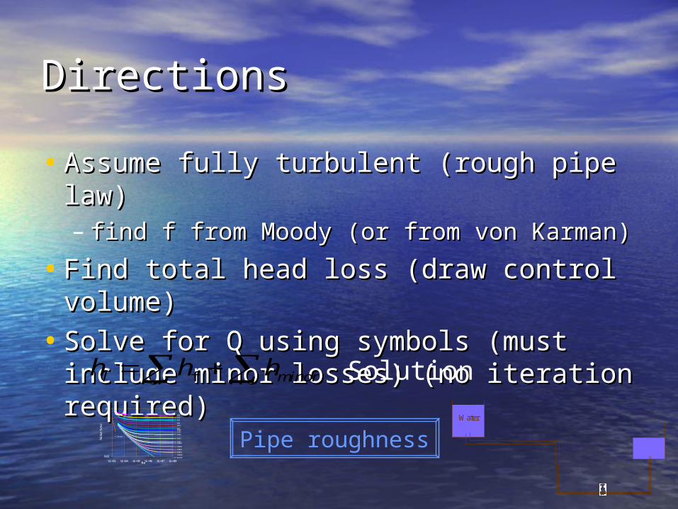
DirectionsDirections

• Assume fully turbulent (rough pipe Assume fully turbulent (rough pipe law)law)– find f from Moody (or from von Karman)find f from Moody (or from von Karman)

• Find total head loss (draw control Find total head loss (draw control volume)volume)

• Solve for Q using symbols (must Solve for Q using symbols (must include minor losses) (no iteration include minor losses) (no iteration required)required)

0.01

0.1

1E+03 1E+04 1E+05 1E+06 1E+07 1E+08Re

fric

tion

fact

or

laminar

0.050.04

0.03

0.020.015

0.010.0080.006

0.004

0.002

0.0010.0008

0.0004

0.0002

0.0001

0.00005

smooth

Pipe roughness

fl minorh h h Solution

WaterWater

Find Q given pipe systemFind Q given pipe system

fl minorh h h

42

28

Dg

QKhminor

2

2 5

8ff

LQh

g D

2

2 5 4

8fl

Q L Kh

g D D

5 48 f

lghQ

L KD D

WaterWater