Personal Criminal Victimization in the United States: Fixed and Random Effects of Individual and Household Characteristics

Journal of Quantitative Criminology, Vol. 16, No. 4, 2000

Personal Criminal Victimization in the United States:

Fixed and Random Effects of Individual and

Household Characteristics

Andromachi Tseloni1

The present research is concerned with multilevel modeling of personal victimiz-ation rates. Data from the 1994 National Crime Victimization Survey areemployed. Following the routine activities and lifestyle victimization theory, indi-viduals’ profile and lifestyle as well as characteristics of their household comprisethe set of explanatory variables. The results of estimated multilevel negativebinomial models, which explicitly disentangle the unexplained heterogeneitybetween individuals and between households, are discussed. The estimated ran-dom effects of household characteristics show that the unexplained heterogeneityfor the average number of personal crimes differs across household types.Further, the individual covariates with between households random effectsbecome less influential the more the base personal crime rates are high.

KEY WORDS: personal crimes; incidence; multilevel negative binomial model;random effects; household heterogeneity.

1. INTRODUCTION

Multilevel models are increasingly implemented in social researchowing to, among other things, their ability to take into account the contex-tual realities of social phenomena, i.e., avoid atomistic or ecological fallacy(Goldstein, 1995), and the recent wide availability of purpose built software.Victimization studies, however, have been left out of this trend despite thefact that clustering of crime experiences exists at a number of levels, namely,the individual, household, neighborhood, etc. Should these levels be takeninto account in empirical research, the integration and improvement oftheoretical approaches would benefit greatly.

For instance, repeat victimization (Pease, 1998), whereby few victimsexperience the majority of crime incidents, implies clustering of such events

1Department of Criminology and Criminal Justice, University of Maryland, 2220 LeFrak Hall,College Park, Maryland 20742. e-mail: [email protected].

415

0748-4518001200-0415$18.000 2000 Plenum Publishing Corporation

Tseloni416

within the same individual if it refers to personal crime or the same house-hold if it is from property crime. Wittebrood and Nieuwbeerta (1999)employed multilevel modeling to study victimization risks per year duringone’s life course using a retrospective life-course Dutch national crime sur-vey. They concluded that risks of repeat victimization during one’s lifecourse are randomly distributed across individuals. The effects of previousvictimization on subsequent victimization are due to unobserved heterogen-eity in the population rather than state dependence (Wittebrood andNieuwbeerta, 1999). Other research has, however, evidenced that previousvictimization during roughly a 5-year reference period significantly increasesthe risk (Ellingworth et al., 1997) and mean number of subsequent incidentsover and above the population unexplained heterogeneity (Osborn andTseloni, 1998). Therefore, the nature of repeats depends on the length ofthe spell and the multilevel specification offered new insights.

Another well-established finding of victimization research asserts thatcrime is clustered within neighborhoods (Sherman, 1989; Trickett et al.,1992). Rountree et al. (1994) employed hierarchical modeling on violentcrime risks of individuals and burglary risks of households clustered withinneighborhoods in Seattle. Their findings supported that both neighborhoodand individual characteristics explain victimization and that the former fac-tors may condition the effects of the latter. They concluded that ‘‘the basicpremises of multilevel analysis . . . are soundly affirmed by our analyses, asis the utility of hierarchical linear model techniques’’ (Rountree et al., 1994,p. 410). Rountree and Land (1996) extended the above work to include clus-tering of neighborhoods within Census tract.

A level of aggregation for personal crimes which lies between theindividual and the neighborhood is the household. It is of substantialinterest to explore whether personal victimizations are disproportionatelyconcentrated on members of the same households by explicitly accountingfor the clustering of individuals within households. Further, the role ofhouseholds on personal victimization ought to be investigated. Fewhousehold characteristics, for instance, income (Kennedy and Forde,1990), composition (Maxfield, 1987) and-inner city residence (Miethe andMeier, 1990), are known to be significantly related to personal victimizationrisk. Unlike research on property victimization and offending, the signifi-cance of household profile and socioeconomic status on personal victimiz-ation has not been fully tested to date. Another issue which deserves specialattention concerns the possible distribution of the effects of personal andhousehold characteristics on victimization across households. Testingwhether random effects exist for personal crimes and, if so, what their impli-cation is for victimization research and crime prevention is a critical issue

Personal Criminal Victimization in the U.S. 417

which has not been addressed by previous research. Should they exist, suchrandom effects are an indication of unexplained heterogeneity betweenhouseholds.

Quantitative victimization research to date has focused on inter-preting the estimated coefficients, also called fixed effects, of empiricalmodels and discussing their implications for theory andor crime preven-tion. Random effects have hardly been explored, let alone interpreted, invictimization literature. Random effects are, however, important forassessing whether the estimated fixed effects are uniform or hold onlyfor some groups of individuals. For instance, the common finding thatmales are more victimized than females may not hold for all types ofhouseholds or in all kinds of neighborhoods. It might be that for some, say,household types both males and females face similar crime risks, whereasfor others men are indeed more victimized (by a factor given by the corre-sponding coefficientfixed effect of an empirical model). If this is so, crimeprevention policies would greatly benefit from differentiating betweenhouseholds with large estimated fixed effects and households where thespecific personal characteristic, in this instance sex, is not critical. For theformer pool of households the estimated coefficients could be used as a ruleof thumb to allocate resources. For the latter both sexes should receiveequal attention for crime prevention.

To my knowledge, Rountree et al. (1994), Rountree and Land (1996),and Wittebrood and Nieuwbeerta (1997) are the only empirical victim-ization studies which employ multilevel or hierarchical modeling of victimiz-ation risks.2 However, the discussion in these pioneer studies is notconcerned with analyzing the random effects of their models. Further, byfocusing on victimization risks rather than counts, they are agnostic of thedistribution of crime events and, therefore, crime concentration.

At this stage it might be helpful to introduce two concepts. Crimeprevalence (CP) is the proportion of victims in the population. It is mostcommonly known as crime risks and interpreted as the observed probabilityof being victimized. If V is the number of victims and N the population ofinterest, CPGVN. Crime incidence (CI ) is the average number of crimesin the population. This is more widely known as crime rates. If C is thenumber of crimes, CIGCN. Understandably crime concentration equalsCICPGCV, namely, the average number of crimes per victim (Tseloniand Pease, 1999). The vast majority of empirical victimization research todate is concerned with crime prevalence.

2Lynch and Berbaum (1997) and Sousa (1998) are in the process of publishing their hierarchicalmodeling of burglaries using the longitudinal file of the NCS and the ICVS, respectively.

Tseloni418

Osborn and Tseloni (1998) have shown that modeling crime incidencerather than risk predicts the entire distribution of victimization incidentsand explicitly accounts for the crime concentration previously identified bydescriptive studies (Ellingworth et al., 1995; Farrell, 1992). To this end, theyuse the negative binomial model (Cameron and Triveldi, 1986) for countsof property crimes, which relaxes the assumption of random events entailedin the Poisson distribution. Using the 1992 British Crime Survey (BCS),their models predict that crime concentration is most marked and victimiz-ation risks are rather misleading when the average crime rates are high(Osborn and Tseloni, 1998, p. 325). Tseloni (1995) studied the distributionof threats in the 1982, 1984, and 1988 BCS using also the negative binomialmodel. While they account for the unexplained heterogeneity in the popu-lation (Osborn and Tseloni, 1998, p. 308), both studies ignore the contextualhierarchies in their data.

In this work I attempt to fill the aforementioned gap in the literatureby using multilevel modeling3 on personal crime counts to estimate the fixedand between-households random effects of personal and household attri-butes. To be more explicit, the goal of this study is threefold. First, it willtest the relevance of a number of household characteristics for personalvictimization controlling for the individual covariates suggested by theoryand previous empirical research. Second, it will model the entire distributionof personal crimes. The statistical approach of previous studies (Osbornand Tseloni, 1998; Tseloni, 1995), namely, the negative binomial regressionmodel, will be improved by using a more flexible specification (see Section5) and explicitly accounting for the clustering of individuals within house-holds. The units of analysis will, thus, be two, individuals (level 1) nestedwithin households (level 2), a structure which has not yet been examined inempirical victimization research. Finally, the study will estimate and inter-pret any between-households random effects of personal and householdcharacteristics while, of course, considering the estimated fixed effects. Suchrandom effects will shed some light on the unexplained household hetero-geneity with implications for victimization theory and crime prevention.

The next section gives a brief overview of the criminal victimizationtheory. The data for this study are taken from the 1994 National CrimeVictimization Survey, which is outlined in Section 3. There follows a dis-cussion of the observed frequency distribution of personal crimes and anoutline of the employed explanatory variables (Section 4). The statisticalmodel is presented in Section 5. Section 6 gives the results of the estimatedmodels. The concluding Section 7 discusses the findings and offers somesuggestions for future research.3The term multilevel is equivalent to hierarchical. It is preferred here because it also refers tothe statistical package used for the analysis (see Section 6.1).


2. VICTIMIZATION THEORY

The modeling exercise of this study follows the routine activities orlifestyle theory of criminal victimization.4 Proponents of both theories(Hindelang et al., 1978; Cohen and Felson, 1979; Garofalo, 1987; Felson,1998) argue that the demographic and socioeconomic characteristics of indi-viduals and their households as well as their lifestyle patterns and everydayroutine activities determine their exposure to crime. With respect to personalcrime, they do so by influencing individuals’ chances of coming into contactwith motivated offenders in the absence of effective guardians.

While lifestyle, which may entail adaptations to role expectations andstructural constraints, directly affects one’s exposure to high criminal vic-timization opportunities, demographic and socioeconomic characteristics doso through associations. This is because according to the theory social con-tacts occur disproportionately among people who share similar attributes.Thus those who have the same demographic and socioeconomic character-istics with offenders of personal crime are expected to be at high victimiz-ation risk. From the offenders’ perspective, individual and householdcharacteristics and lifestyles determine target suitability and desirability.

The lifestyleroutine activities theory has been supported and improvedby empirical evidence (i.e., Maxfield, 1987; Kennedy and Forde, 1990;Rountree et al., 1994). This study employs the set of explanatory variables(see Section 4.2) which both the theory and the relevant previous empiricalresearch suggest.

3. THE DATA

As mentioned, the present study employs data from the 1994 NationalCrime Victimization Survey (NCVS). The NCVS is conducted monthly bythe Census Bureau of the United States on behalf of the Bureau of JusticeStatistics. The sample represents in principle the noninstitutionalized perma-nent residents of the United States 12 years or older. The Address List fromthe Decennial Census provides the sampling frame for a rotating panel ofhousing units. The survey collects detailed information about any victimiz-ation experience of each member 12 years or older of the households whichreside in the selected housing units. The reference period is the time elapsedbetween two interviews. Demographic and socioeconomic characteristics ofthe interviewees, their attitudes toward crime and experiences with the policeare also surveyed. The selected housing units remain in the NCVS sample

4The present study is not concerned with testing the social disorganization theory (Shaw andMcKay, 1942; Sampson and Groves, 1989). The data file employed does not permit anyaggregation at the neighborhood level.

Tseloni420

for the total of 3 years and their residents are interviewed every 6 monthsduring that period.

The 1994 NCVS includes information collected during three interviewsbetween January 1994 and June 1995. It thus covers victimization experi-ences and other related issues which occurred during a period of a maximumof 1.5 years. Being a sample of housing units, the NCVS has attrition prob-lems since it does not follow or trace back the households if they move outof or into, respectively, the selected units before the end of the survey.

The sample of this study consists of all the households which occupiedthe selected housing units at the time of the first interview (January to June1994) of the 1994 NCVS.5 Most households (91.3%) in the employed dataset had a bounding interview. This is a unique feature of the NCVS whichensures that no telescoping of the reported incidents has taken place. Thesampling unit is the household with all its members 12 years or older. Thebasic exposure period to victimization is 18 months.

As mentioned in the preamble to this paper, the data set offers a naturaltwo-level hierarchy of individuals (level-1 unit) nested within households(level-2 unit). Table I presents the observed frequency distribution of indi-viduals per household. Clearly the majority of households (95.6%) includesbetween one and four individuals 12 years old or older.

Table I. Number of Individuals 12 Years Old orOlder per Household

Number of individuals Frequency

1 21,6752 71,1933 32,4564 20,0025 6,2066 1,6957 5028 1759 83

10 2311 9

Total 154,019

5Households which moved in after the first interview have been eliminated from the data set.The sampling structure of the NCVS is preserved by relating one household to each originallyselected housing unit. Thus, one avoids overcounting of the housing units which were occupiedby more than one household during the duration of the 1994 NCVS. Additionally, all thehouseholds which had a bounding interview have been kept in the sample.


4. THE VARIABLES

4.1. Personal Victimization

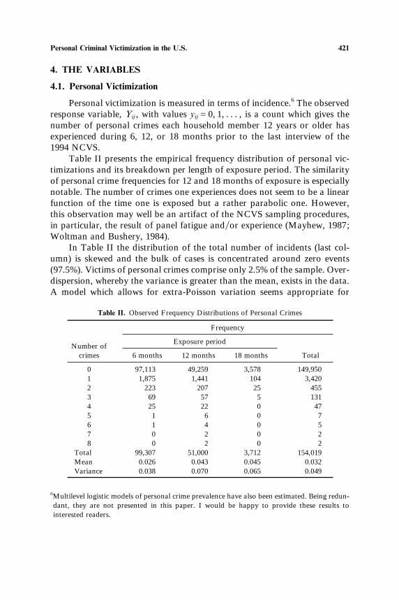
Personal victimization is measured in terms of incidence.6 The observedresponse variable, Yij , with values yijG0, 1, . . . , is a count which gives thenumber of personal crimes each household member 12 years or older hasexperienced during 6, 12, or 18 months prior to the last interview of the1994 NCVS.

Table II presents the empirical frequency distribution of personal vic-timizations and its breakdown per length of exposure period. The similarityof personal crime frequencies for 12 and 18 months of exposure is especiallynotable. The number of crimes one experiences does not seem to be a linearfunction of the time one is exposed but a rather parabolic one. However,this observation may well be an artifact of the NCVS sampling procedures,in particular, the result of panel fatigue andor experience (Mayhew, 1987;Woltman and Bushery, 1984).

In Table II the distribution of the total number of incidents (last col-umn) is skewed and the bulk of cases is concentrated around zero events(97.5%). Victims of personal crimes comprise only 2.5% of the sample. Over-dispersion, whereby the variance is greater than the mean, exists in the data.A model which allows for extra-Poisson variation seems appropriate for

Table II. Observed Frequency Distributions of Personal Crimes

Frequency

Exposure periodNumber of

crimes 6 months 12 months 18 months Total

0 97,113 49,259 3,578 149,9501 1,875 1,441 104 3,4202 223 207 25 4553 69 57 5 1314 25 22 0 475 1 6 0 76 1 4 0 57 0 2 0 28 0 2 0 2

Total 99,307 51,000 3,712 154,019Mean 0.026 0.043 0.045 0.032Variance 0.038 0.070 0.065 0.049

6Multilevel logistic models of personal crime prevalence have also been estimated. Being redun-dant, they are not presented in this paper. I would be happy to provide these results tointerested readers.

Tseloni422

modeling the response variable, personal crimes (Cameron and Trivedi,1986; McCullagh and Nelder, 1989).

4.2. Explanatory Variables

To model personal victimization a number of characteristics of the indi-viduals and their households from the 1994 NCVS are employed. Thecovariates which refer to the individual (level 1) include sociodemographiccharacteristics, such as sex, age, race, marital status, educational level, andemployment status, as well as lifestyle factors, namely, shopping, eveningsout and use of public transportation. The more outgoing a life one leads,the more he or she is expected to come into contact with potential offendersunder conditions conducive to high opportunities of victimization.Additionally, this pattern is likely to be followed by people who have atleast one of the following attributes: male, young, black, not married, unem-ployed, and of low socioeconomic status (Hindelang et al., 1978, p. 257).However, in practice, educational level has been found to be positivelyrelated to victimization. This is due to the increased ability of more educatedrespondents to identify, recall, and report a crime event in a survey (Hough,1987, p. 10). Length of time living at the address provides and indicator ofguardianship through knowledge of the neighborhood and informal socialcontrol.

Household characteristics which are defined at level 2 include indicatorsof affluence, household composition, and protection against crime. In themodels below affluence is indicated by the number of cars owned, annualfamily income, tenure, and type of accommodation. The more affluent oneis, the less he or she is expected to be the victim of personal crime, owingto lack of physical and social proximity to potential offenders. A large num-ber of cars in a household may, on the other hand, indicate a high mobilityto out-of-family activities of its members and, thus, an anticipated positiverelationship to personal crime.

Household composition, given in the models by children under 12 yearsold in the household and number of adults,7 depicts vulnerability and guard-ianship, respectively. Protective measures include whether devices againstintruders are fitted and participation in neighborhood watch. Although, inprinciple, both are expected to decrease victimization, the direction of caus-ality is unclear in cross-section designs. Protective measures may be a reac-tion to high crime, thus, portraying an unexpected positive relationship withvictimization through higher such opportunities.

7For convenience individuals 12 years or older are referred to as adults throughout this studyaccording to the NCVS respondents’ age. In fact respondents younger than 18 years oldcomprise 10.5% of the employed sample.


Place size in terms of population and an urban dummy variable aretwo household-level covariates related to the area of residence. According totheory, people living in urban or highly populated areas are more frequentlyexposed to crime than others due to physical proximity to potential

Table III. Description of Covariates

Variables Mean (SD) Value

Individual-level covariatesAge 43.07 (19.30) 12–90Male 0.461 0–1Marital status

Married (base) 0.561 —Single 0.268 0–1Divorced 0.099 0–1Widowed 0.072 0–1

RaceCaucasians (base) 0.872 —African-AmericanNative AmericanAleutEskimo 0.103 0–1AsianPacific Islander 0.025 0–1

Educational attainmentPrimary school or illiterate (base) 0.121 —High school 0.466 0–1College 0.413 0–1

Employment statusWorking full-time (base) 0.570 —Working part-time 0.038 0–1No paid work 0.320 0–1School pupil 0.072 0–1

Going shoppingNever (base) 0.020 —Daily 0.200 0–1Once a week or less often 0.780 0–1

Spending evenings outNever (base) 0.077 —Daily 0.193 0–1Once a week or less often 0.730 0–1

Using public transportationNever (base) 0.802 —Daily or at least once a week 0.066 0–1Less often than once a week 0.132 0–1

Length of time at addressLess than 6 months 0.031 0–1Six to 11 months 0.045 0–1One or 2 years 0.141 0–1Three to 5 years 0.201 0–1Six to 10 years 0.192 0–111 years or longer (base) 0.390 —

Tseloni424

Table III. Continued.

Variables Mean (SD) Value

Household-level covariatesChildren in the houshold 0.303 0–1Number of adults 2.52 (1.14) 1–11Number of cars

None (base) 0.065 —One to 3 cars 0.786 0–14 or more cars 0.149 0–1

Household annual incomeLess than $10,000 0.103 0–1$10,000–$49,999 (base) 0.547 —$50,000 or more 0.244 0–1Refused to answer 0.106 0–1

Tenure: own houseapartment 0.235 0–1Type of accommodation: houseapartmentflat 0.936 0–1Devices against intruders 0.642 0–1Neighborhood watch member 0.098 0–1Urban area 0.697 0–1Place size

24,999 or less (base) 0.612 —25,000–249,999 0.249 0–1250,000 or more 0.139 0–1

Exposure period6 months 0.645 0–112 months 0.331 0–118 months (base) 0.024 —

Number of cases 154,019

offenders in the absence of capable guardians. Place size and urban are,therefore, expected to be positively related to personal victimizations.

To sum up, personal crimes in the models below is a cumulative countof such events within the total period of participation in the 1994 NCVS.All covariates are measured at the time of the last interview. Thus theemployed data are essentially cross sectional.

Table III describes the covariates used in this study, giving their mean,standard deviation (SD), where appropriate, and range of values. They areall qualitative (binary, nominal, or ordinal) except for age and the numberof adults, which are discrete variables. In Table III the reference categoriesof the nonbinary qualitative covariates are indicated as the base. They arepresented in parentheses after the variable name in the table of modelingresults.

Two dummy variables, 6 and 12 months, which are defined at the per-son level, capture the effect of shorter reference periods for those whomoved before the end of the 1994 NCVS. Recent research based on the


NCVS shows that moving is related only to property crime (Dugan, 1999).Personal victimization may not affect moving decisions for several possiblereasons. To avoid revictimization, victims may follow less extreme lifestyleadjustments than moving home. Personal or violent crime may not induceto the victim fear of crime, high-risk considerations, or enough motivationto move out of the neighborhood because it is not as impersonal in natureas property crime is (Dugan, 1999). Therefore, the next models of personalvictimization are unlikely to entail any bias due to moving. Since theobserved frequency distributions of personal crimes during 12 and 18months are quite similar (see Table II), it is expected that only 6 monthswill have a significant differential effect on the mean number of personalcrimes.

5. THE STATISTICAL MODEL

Goldstein (1995) describes multilevel models for proportions and pre-sents models for counts as an extension of the former. The multilevel nega-tive binomial model derives in a straightforward manner as an extension ofthe Poisson. First, the multilevel Poisson model is defined.

Let µi j be the expected number of personal victimizations. The log linkfunction for the Poisson model with random coefficients is

ln µijGη ijGXijβC ∑p

τG0

uτ j zτ ijC ∑r

τGpC1

uτ j zτ j ,

iG1, . . . , 11, jG1, . . . ,H (1)

where τG0, 1, . . . , r, with r being the total number of random coefficientsin the model including the intercept. Xij is a row vector of K (K¤r) covariatesfor the ij th individual, including the intercept, some of which may refer tothe individual’s household. z0ijG1, zτ ijGxτ ij , for τG1, . . . , p, are the covari-ates with random effects for the ij th individual. zτ jGxτ j , for τGpC1, . . . , r,refer to the r–p random effects covariates for the j th household.[uτ j ] ∼ N(0, Ωu ) is the random departure from the j th household (Goldstein,1995).

The probability distribution for Yij follows the Poisson distribution sothat the probability that Yij takes the specific value yij is

Pr(YijGyij )Gexp(−µij )µyij

ij

yij !, yijG0, 1, . . . (2)

with the usual property that E(Yij )Gvar(Yij )Gµij , which equals exp(η ij )from (1).

Tseloni426

The multilevel negative binomial model (MNBM) derives by allowingfor between-level-1 units random variation of the expected number ofevents µij in (2).

ln µijGη ijCeij (3)

where cov(eij , uij )G0 and exp(eij ) or µij follows a gamma probability distri-bution, Γ(ϕij , νij ), with E(µij )Gϕij and var(µij )G(1νij )ϕ 2

ij (Cameron andTrivedi, 1986, p. 32). Integrating with respect to eij the resulting probabilitydistribution,

Pr(YijGyij )Gexp(−exp(η ijCeij )) exp(η ijCeij )

yij

yij !(4)

the MNBM is obtained:

Pr(YijGyij )GΓ( yijCνij )

yij !Γ(νij )

ννijij ϕ yij

ij

(νijCϕij )νijCyij

, yijG0, 1, . . . (5)

where E (Yij )Gϕij and var(Yij )GϕijC(1νij )ϕ 2ij (Cameron and Trivedi, 1986,

p. 33).If we assume that ϕij is proportional to exp(η ij ) from Eq. (1), in particu-

lar, if ϕijGα exp(η ij ) with αH0, and that νijGνGα2γ, thenE (Yij )GαµijGµ*ij and var(Yij )GαµijCγ µ2

ijGE (Yij )[1C(1ν)E (Yij )]. Thuswe obtain one version of the MNBM with extra negative binomial variation.

The MNBM is defined in the software package MLwiN by specifyingthe observed response as:

YijGµijCε0ijµ0.5ij Cε1ijµij (6)

where E (ε0ij )GE (ε1ij )G0, σ2ε0Gα , σ2

ε1Gγ, and cov(ε lij , uτ j )G0, for eachlevel-1 random component (lG0, 1).

The extra-Poisson variation at level 1 is given by α, γ , and µij . Sinceα, γH0, the model allows for overdispersion. Overdispersion here isassumed to stem from unexplained heterogeneity (Osborn and Tseloni,1998, p. 308) between individuals and is given by 1ν.

6. RESULTS

6.1. General Remarks

Table IV presents the estimated MNBM for personal crimes. Two mod-els are presented here. Model 4.1, which is displayed in the second columnin Table IV, is a model of fixed effects with a random intercept. Model 4.2,given in the third column, includes between-households random effects of


the household and individual-level covariates. Having originally includedall the variables given in Table III, the ones with estimated coefficients at a1.4 t statistic or larger were kept in the models discussed here. If the coef-ficient of at least one category of a nonbinary qualitative variable passed

Table IV. Multilevel Negative Binomial Models of Personal Victimizationa

Covariate Model 4.1 Model 4.2

Estimated individual-level fixed effects (SE)Individual characteristicsAge A0.033 (0.002) A0.034 (0.002)Male 0.353 (0.035) 0.360 (0.036)Marital status (married)

Single 0.430 (0.057) 0.425 (0.058)Divorced 0.942 (0.058) 0.930 (0.060)Widowed 0.379 (0.127) 0.376 (0.127)

Race (white)African-AmericanNative AmericanAleutEskimo A0.065 (0.057) A0.078 (0.056)AsianPacific Islander A0.483 (0.128) A0.496 (0.127)

Educational attainment (primary schoolilliterate)High school A0.014 (0.068) A0.024 (0.067)College 0.102 (0.075) 0.094 (0.075)

Employment status (working full-time)Working part-time 0.318 (0.076) 0.309 (0.076)No paid work A0.021 (0.050) A0.029 (0.049)School pupil 0.239 (0.077) 0.226 (0.077)

Individuals’ lifestyleShopping (never)Daily 0.543 (0.178) 0.557 (0.178)Once a week or less often 0.216 (0.175) 0.238 (0.175)

Evenings out (never)Daily 0.364 (0.094) 0.341 (0.093)Once a week or less often 0.049 (0.089) 0.040 (0.089)

Public transportation (never)Daily or at least once a week 0.453 (0.062) 0.444 (0.062)Less often than once a week 0.279 (0.048) 0.281 (0.048)

Length of time at address (11 years or longer)Less than 6 months 0.903 (0.080) 0.893 (0.081)Six to 11 months 0.485 (0.076) 0.466 (0.077)One or 2 years 0.213 (0.058) 0.211 (0.058)Three to 5 years 0.047 (0.055) 0.051 (0.055)Six to 10 years 0.085 (0.056) 0.080 (0.055)

Exposure period (18 months)6 months A0.785 (0.104) A0.780 (0.104)12 months A0.134 (0.104) A0.138 (0.105)

Joint χ2 test of individual characteristicsfixed effects 2,368.071 2,359.894

Degree of freedom 25 25

Tseloni428

Table IV. Continued.

Covariate Model 4.1 Model 4.2

Estimated household-level fixed effects (SE)Household characteristicsChildren 0.183 (0.042) 0.178 (0.042)Number of adults A0.049 (0.018) A0.050 (0.018)Number of cars (none)

One to 3 cars A0.057 (0.077) A0.033 (0.075)4 or more cars 0.207 (0.093) 0.233 (0.090)

Household annual income ($10,000–$49,999)Less than $10,000 0.179 (0.062) 0.162 (0.061)$50,000 or more A0.067 (0.047) A0.063 (0.047)Refused to answer A0.062 (0.065) A0.063 (0.066)

Devices against intruders 0.184 (0.041) 0.175 (0.040)Neighborhood watch 0.129 (0.059) 0.134 (0.057)Area characteristics

Urban 0.212 (0.050) 0.217 (0.052)Place size (24,999 or less)25,000–249,999 0.109 (0.047) 0.123 (0.047)250,000 or more 0.241 (0.056) 0.236 (0.055)

Joint χ2 test of household characteristicsfixed effects 149.329 153.777

Degrees of freedom 12 12Constant A3.211 (0.263) A3.211 (0.263)Mean personal victimizations 0.009 0.009

(reference individual)Estimated random effects (SE)

Between individualsα 1.149 (0.006) 1.183 (0.007)γ 3.565 (0.190) 2.935 (0.263)

Between householdsσ2

Constant 1.852 (0.122) 7.705 (0.435)σ2

6 months 1.679 (0.701)σConstant, 6 months A0.614 (0.359)σ2

Male 2.254 (0.457)σConstant, male A1.778 (0.266)σ2

Single 4.341 (0.472)σConstant, Single A3.441 (0.291)σ2

Shopping daily 1.363 (0.498)σConstant, shopping daily A1.143 (0.252)σ2

Evenings out daily 0.935 (0.465)σConstant, evenings out daily A1.030 (0.244)σConstant, one to 3 cars 0.518 (0.093)σConstant, $50,000 or more 0.298 (0.109)σConstant, refused to answer 0.585 (0.177)σConstant, neighborhood watch A0.476 (0.124)σConstant, urban A0.975 (0.135)σConstant, 250,000 or more A0.369 (0.102)

Joint χ2 test of random effects 508.999Degrees of freedom 16

aThe number of observations is 154,019.


the above threshold, then all its categories were retained. Tenure and typeof accommodation were, thus, dropped from the final models. Table IVpresents the estimated fixed and random effects, with their correspondingstandard errors in parentheses.

Whether to include any random effects of covariates, here variancesand the covariances with the intercept, in Model 4.2 was determined fromthe results of the corresponding Wald hypothesis tests (Goldstein et al.,1998, p. 103). To this end, the critical values of χ 2 tests with one (for anylevel-2 dummy variable) or two (for any level-1 dummy variable, as well asage and number of adults) degrees of freedom at a 0.05 P value have beenused. Thus, the covariates which gave either nonsignificant or zero randomeffects do not contribute to the random components part of Model 4.2.

Table IV has three parts: the first and the second display the estimatedfixed effects of the personal and household characteristics, respectively, andthe third the estimated random components of the models. Joint χ 2 testsfor the included fixed or random effects with their appropriate degrees offreedom are given at the end of each part of Table IV. In comparison withχ 2 distributions with 25, 12, and 16 degrees of freedom, the correspondingindividual and household fixed effects and their random components arehighly statistically significant, implying that each set of covariates as wellas their random effects adds important information for the prediction ofpersonal crime victimizations.

The estimated models have been obtained using iterative generalizedleast squares (IGLS) estimation with first-order marginal quasi-likelihood(MQL) approximation via the software package MLwiN (Goldstein et al.,1998).

Before moving into the actual discussion of the estimated results, Ishould mention that the majority of personal crimes reported in the 1994NCVS are assaults or threats. Sexual assaults, which are experienced mostlyby women, comprise an absolute minority of just 162 victims and 182 inci-dents in the entire data set. Domestic crime may be seriously underrepres-ented and the following results possibly highlight the characteristics of thevictims of the predominant types of personal crimes in the analysis.

6.2. Fixed Effects

The estimated MNBM of personal crime incidence generally supportthe lifestyleroutine activities theory. Most coefficients are highly signifi-cant. As mentioned, the first two parts of Table IV display the estimatedindividual and household fixed effects of the MBNM, respectively.

From Eq. (1) it follows that the intercept is the (natural) logarithm ofthe mean number of events when all covariates and between-households

Tseloni430

random components become zero. In the presence of qualitative covariates,the intercept refers to the individual who is described by all the referencecharacteristics of such variables and zero values of the quantitative ones,here age and number of adults. For the models in Table IV the referenceindividual is a white, married woman with an elementary education whoworks full-time and never goes out shopping or spends any evenings out oruses public transportation. She has lived for more than 11 years at the sameaddress in a nonurban area with a population of less than 25,000. There areno children or cars in her household, which earns between $10,000 and$49,999 per annum. Her house is not protected against crime via neighbor-hood watch or devices against intruders. To ease interpretation, Table IV(end of second part) presents the predicted average number of personalcrimes for this reference individual assuming that she is of average age (43years old) and she lives with another adult. The displayed value of 0.009,which is calculated as [exp(−3.211A(0.033 ∗ 43)A(0.049 ∗ 2)], indicatesthat the reference woman is effectively expected to experience zero personalcrimes during an 18-month period. This (unit specific) prediction is basedon zero random effects.8

The estimated fixed effects of the individual and household covariatesare now discussed. Their exponentials, exp(bk ), give the multiplicative factorby which the base average number of crimes (0.009) is modified as a result ofthe corresponding attribute, xkij , assuming that all other covariates remainconstant. For instance, being divorced increases the average number of per-sonal crimes by 2.56 (calculated as exp(0.942)) compared to being mar-ried, and therefore, divorced people suffer 156% more personal crimes thanmarried people of otherwise identical characteristics. The following dis-cussion focuses on the results of the fixed effects model (Model 4.1) andassumes no random variation.

Considering the individual-level covariates, the coefficient of age indi-cates that the number of personal crimes one experiences decreases by 3%per year he or she grows older. Men suffer 42% more personal crimes than

8In multilevel models two types of predictions apply: unit specific (US) and population averag-ing (PA). The US prediction given above effectively ignores the between-households randomeffects. Its corresponding expected var(Yij )G0.011. The PA prediction from the models ofthis study requires evaluating Eln µi jGη i jGXi jβC∑p

τG0 uτ j zτ i jC∑r

τGpC1 uτ j zτ j over u. Thisis done using a Taylor series second-order approximation and taking expectations,[exp(Xijβ)Cσ2

u [exp(Xijβ)]2, where β can be substituted by the estimated fixed effects, b, andσ2

u by the estimated σ2constant . For instance, the PA prediction of the average number of per-

sonal crimes gives expected µG0.017 and 0.044 from Model 4.1 and 4.2, respectively. Thecorresponding estimated var(Yij )G0.021 and 0.058. As shown, the PA prediction from Model4.2 is the one closest to the observed mean and variance of personal crimes given in Table II(0.045 and 0.065). For a detailed discussion of prediction in multilevel modeling, see Goldstein(1995) and Goldstein and Rasbash (1996).


women with otherwise similar sociodemographic profile, lifestyle, andhousehold characteristics.

Married individuals are less likely to associate with people outside theirfamily and immediate friends’ environment, thus becoming less exposed tocrime than those who are not married (Sampson and Laub, 1993; Warr,1998). Indeed, divorced has the highest effect among all the characteristicsconsidered in the model, whereas single and widowed show also nontrivialincreases of personal crimes of 54 and 46%, respectively.

With respect to race, Asians or Pacific Islanders are 48% less likely tosuffer personal crimes than Caucasians, which is not unexpected. Asian-Americans, despite being ethnically and historically heterogeneous, adhereto the common Asian values of family, education, hard work, and respectfor elders (Kibria, 1997), which provide a protective network against highexposure to crime unless they are unfortunate in their family. The lack ofeffect of African-American or American Indian on personal crimes seemssurprising. However, it may not be without explanation. First, personalcrimes of some seriousness are more likely to aggravate to homicide, whichis evidently not captured in self-report victimization surveys (Lattimore etal., 1997, p. 138). Second, if the incidents are nonserious, they may be con-sidered too trivial by the victim, who may thus not report them in theNCVS.9 Third, the high victimization of African-Americans might be duesolely to poverty or type of area they live in and not at all a race effect. Inongoing research which employs the 1995 NCVS to model violent crime,Lauritsen and Sampson (1999) argue that, once controlling for householdand neighborhood income, black becomes nonsignificant. Indeed, the mod-els presented here affirm that household annual income less than $10,000and urban andor place size greater than 250,000 people significantlyincrease the mean number of personal crimes (see this section below),whereas African-American is irrelevant to the dependent variable.

People with college education report 11% more personal crimes thanthose who have attended elementary or no school. This effect should betreated with suspicion: as mentioned, it may be an artifact of the ability ofeducated people to identify events of criminogenic nature and to respondeffectively to complex surveys, such as the NCVS (Hough, 1987).

Working part-time and school pupil show nontrivial positive effects onthe mean number of personal crimes, 37 and 27%, respectively. Someschools are indeed far from safe environments (Whitaker and Bastian, 1991;

9Apart from the possibility of underreporting their victimization experiences African-Ameri-cans, especially young males, may have higher nonresponse rates compared to Caucasians inthe NCVS (personal communication with Professor Jim Lynch). Having said that, however,reverse record checking of the NCS data (older version of the NCVS) showed no significantcorrelation between response bias and respondent characteristics (Schneider, 1981).

Tseloni432

Sherman, 1999). Part-time working in the NCVS refers to people who movefrequently in and out of the labor market and thus may take up unstableor low-status jobs. Their route to personal victimization may be twofoldthrough job associations and (extended) leisure time.

Length of residence at the same address is inversely related to personalvictimization. The longer one lives at the same address the more he or shebecomes familiar with the neighborhood and, therefore, can protect oneselfagainst crime. The limit seems to be 3 years since people living at the sameaddress between 3 and 10 years do not effectively experience any more per-sonal crimes than those living at the same address for at least 11 years. Incontrast, less than 6 months increases the number of personal crimes by147%, which is the second highest effect in the entire model after divorced.Further, 6 to 11 months and 1 to 2 years increase personal crimes by 62and 24%, respectively, compared to the base category.

The results on individuals’ lifestyles indicate that habitual outgoingactivities increase the frequency of personal crimes by bringing people intocontact with potential offenders. In particular, going shopping or spendingthe evening out daily have considerable positive effects on personal crimes(72 and 44% respectively). It is clearly daily outgoing activities that affectpersonal victimizations, not the less frequent ones.

Using public transportation at any rate also increases personal crimes(57 and 32%). Public transportation exists most in the (metropolitan and)urban areas of the United States and is plausibly used by those who cannotafford a car. Given that annual family income, area size, and number ofcars are individually included in the model, it seems that a separate effectof public transportation exists perhaps by providing the scenery for personalvictimization.

Apart from individual characteristics and lifestyles, household-levelcovariates are important predictors of personal victimization partly becausehousehold composition and economic status suggest constraints, or lackthereof, on individuals’ behavior. They also define individuals’ associations.Considering the household composition, children in the family increase thenumber of personal victimizations experienced by any adult (see footnote7) member by 20%. Number of adults decreases personal victimizations by5% per adult added in the household. Household members are likely tospend much of their leisure time together, thus avoiding association withandor being guarded against potential offenders (Hindelang et al., 1978)unless they are unfortunate in who they live with.

Four or more cars are possessed by households of either many youngadults who share accommodation or a family with at least two adult chil-dren living at home. Whatever the case, it is (unlike earned income) a visiblesign of relative affluence. Individuals in households owning four or more


cars suffer 23% more personal crimes than those in the base category of nocars. Counteracting the crime averting effects of many adults, members ofhouseholds with four or more cars are likely to spend considerable timeaway from home or family, thus, be frequently exposed to potentialoffenders in the absence of capable guardians (Cohen and Felson, 1979).

Low household annual income (less than $10,000) brings about an esti-mated 20% increase of the mean for personal crimes. Being poor also indi-cates living in deprived and, therefore, high-crime areas. On the other hand,living in a household with $50,000 or more per annum shows a nonsignifi-cant negative effect on the mean number of victimizations. As shown in thenext section, household affluence has significant random effects.

Participating in neighborhood watch and installed devices againstintruders may also appear in high-crime areas, hence, the respective 14 and20% positive effect on personal victimizations. Neighborhood watchscheme, if effective at all (Bennett, 1990; Skogan, 1990), is geared towardpreventing property and not personal crimes. As already discussed (Section4), the direction of the effects of neighborhood watch and protection devicesis confounded in cross-sectional data.

Households’ area of residence is another significant predictor of crimesince the latter occurs in impersonal andor large communities and the innercities. Living in an urban area or in one of 250,000 people or more increasespersonal crimes by 24 and 27%, respectively. The place size results indicatethat the larger the community, the higher victimization rates its inhabitantsface.

The effect of the shorter reference period for individuals who movedout before the end of the survey indicates that victimization rates are aparabolic function of the exposure period. When the reference perioddecreases by one-third the average number of personal crimes decreases by13%, while a two-thirds reduction of the former more than halves (54%) theaverage number of personal crimes. As mentioned, such a relationshipbetween number of personal crimes and exposure period may be simplythe result of panel fatigue andor experience due to the NCVS procedures(Woltman and Bushery, 1984).

6.3. Unexplained Heterogeneity and Other Random Effects

As mentioned in Section 5, the level-1 random component consists ofthe Poisson (expected) mean number of personal victimizations, µ, and theoverdispersion parameters, α and γ , which are a measurement of unex-plained heterogeneity between individuals with regard to their personal vic-timization rates. The estimated overdispersion from Model 4.1 is 2.70[calculated as 3.565(1.149)2]. In the MNBM specification with random

Tseloni434

effects (Model 4.2), it is 2.11. It might be that some of the unexplainedbetween-individuals heterogeneity can be explained by the between-house-holds random effects of covariates.

The two models of Table IV show effectively identical estimated fixedeffects. The estimated random effects of Model 4.2 are henceforth discussed.Their interpretation relies on the level at which the corresponding covariatesare measured (Goldstein, 1987, p. 37, 1995, p. 51). For the MNBM thebetween-households random variation of the coefficients of householdcharacteristics contrasts variances of average personal crimes for differenttypes of households. These types of households are identified by the corre-sponding household-level dummy variables. The variance of the averagenumber of victimizations for any category of a household variable is givenby the between-households variance of the constant term. This is 1.852 forthe fixed effects model and 7.705 for the random effects model. The varianceof the average number of victimizations for a household type with randomeffects is the variance of the constant plus twice its covariance with thecorresponding dummy variable.

In particular, the variance of the mean for personal crimes for individ-uals in households with one to three cars is larger (8.74 computed as7.705C2(0.518)) than for those in households without a car (7.71),assuming all other characteristics are the same. No car is the base categoryof the corresponding dummy variable. The random variation of the meanfor personal crimes between households with one to three cars is one ofthe highest in the model. It seems entirely justifiable since such householdscomprise a wide range of different types such as a couple with one car inan urban area or one adult with three cars.

The highest random variation of the mean for personal crimes appearsfor people in households with unreported annual income (8.78), whereasthose earning $50,000 or more also show higher than the base variation(8.30). It seems that members of households in crime-averting conditions,such as reported ($50,000 or more, car ownership) or hypothesized (refusedto answer) affluence, have more diversified personal crime rates than others.In other words, personal crime rates seem more erroneous between suchhouseholds than for households without a car or of average income (thebase categories).

At the other end of the scale, inhabitants of urban areas seem to experi-ence the least variable between-households personal crime incidence (5.76calculated as 7.705A2(0.975)). The estimated variances of the mean forpersonal crimes for participation in neighborhood watch (6.75) and highlypopulated (250,000 or more) areas (7.03) are also lower than the variancefor the corresponding base categories. The last three effects indicate thatpersonal crime rates of individuals in households living in high-risk areas


vary less than between the base households. Therefore, members of suchhouseholds face rather similar average numbers of personal crimes thanmembers of households in nonurban or sparsely populated areas or thosewithout formal neighborhood watch.

As mentioned, the interpretation of random effects depends on the levelat which the corresponding covariates are measured. The variance of thecoefficients of individual characteristics is interpreted as the between-house-holds variation of the corresponding fixed effect. Their covariance with theintercept may be used to calculate the level-2 correlation between the inter-cept and the corresponding ‘‘slope’’ (Goldstein, 1995, pp. 31–32, 103) orpartial effect.

All individual-level random effects reported in Model 4.2 show sub-stantial variances and give moderate to high negative correlations betweenthe corresponding fixed effect and the intercept. The effect of male on per-sonal crimes shows variability (2.25) of about six times larger than its fixedpart (0.36). The corresponding estimated correlation with the intercept isequal to A0.43 [calculated as A1.778(2.254 ∗ 7.705)12], indicating that forindividuals in households with high (low) average personal crimes, the dif-ference in such rates between males and females is rather small (large). Sexmatters less or being female protects one less from personal crimes in house-holds which have high such incidence rates compared to households with alow personal crime incidence.

The most marked result among the individual random effects refers tosingle, which has an estimated between-households variance roughly 10times larger than its fixed part. The estimated correlation with the interceptequals A0.59. The higher (lower) the personal crime incidence of householdmembers, the lower (higher) the differential effect of single compared tomarried. In households with a high mean for personal crimes, single peopleare not at much higher risk than married people and the correspondingfixed effect is smaller than the one displayed in Table IV. It is worth notingthat such a trade-off between a household’s base incidence and the magni-tude of the fixed effect does not seem to exist for the other two maritalstatus categories, which showed absolutely no variation.

The random components of shopping daily and evenings out daily areinterpreted in a similar way. They show respective variances roughly twoand three times larger than the corresponding fixed effects. The respectivecorrelations with the intercept are A0.44 and A0.38. Shopping or spendingthe evenings out daily increases the mean for personal crimes less (more)than the corresponding fixed effect for members of households with a high(low) base incidence.

The differential effect of a 6-month compared to an 18-month exposureperiod shows a low (in absolute terms) correlation with the intercept (−0.17).

Tseloni436

For households of a high (low) personal crime incidence, such rates decreaseslightly less (more) as a result of the lower exposure period than for mem-bers of households of low incidence rates.

7. DISCUSSION AND CONCLUSIONS

This paper models the distribution of personal victimizations allowingfor clustering of individuals within-household and between-households ran-dom variation of coefficients. The estimated models offer important newinsights to victimization research, especially through the random effectsspecification, which has been overlooked in previous empirical victimizationstudies. They also show that both individual and household characteristicsare important predictors of personal crime incidence. Before discussing thecentral questions to this study, the most noteworthy fixed effects of individ-ual characteristics are summarized.

Divorced are expected to suffer the highest mean number of personalcrimes perhaps through associations or due to (still?) social stigma. This isan effect consistent with previous research on threats (Tseloni, 1995). Asianor Pacific Islanders, on the other hand, is the least victimized group ofpeople. African-Americans or American Indians are not expected to sufferany more of less personal crimes than Caucasians with otherwise identicalindividual and household attributes. Part-time work or going to schoolincreases the mean for personal crimes, perhaps through both interactionswith potential offenders and lack of time constraints for leisure activities.Progressive knowledge of one’s neighborhood indicated by length of timeat address results in a gradual decline in one’s expected average number ofpersonal crimes. Using public transportation and daily outgoing activities,such as shopping and evenings out, increase them significantly. While theselifestyle effects are of the expected direction, they are not invariable,as shown in Section 6.3. Ignoring this for a moment, the fixed effects ofpersonal attributes and behavior with the exception of race support thelifestyleroutine activities theory of personal victimization.

The remainder of this section discusses the results of the estimatedMNBM in view of the three issues of interest which have been raised in thepreamble to this paper.

• How household characteristics influence the average number of per-sonal victimizations of its members.

• How the multilevel negative binomial specification advances ourunderstanding of victimization.

• What the random effects imply for predicting the mean for personalcrimes.


Considering the first issue, personal victimization incidence does notdepend only on personal attributes of individuals; it is equally influencedby a number of household characteristics. Guardianship through increasingnumber of adults in the household reduces the mean for personal crimes.Poverty (less than $10,000) and urban and densely populated (250,000 ormore) areas of residence as well as increased mobility, which is indicated byfour or more cars, are positively related to personal crimes. Four or morecars seem to have the highest effect on the dependent variable among allthe household characteristics included in the models. To my knowledge,such a relationship has not been evidenced in previous research. It soundlyaffirms the routine activities theory. Children in the household (or lack of)is commonly employed as a proxy for home-oriented (or outgoing) lifestyle(Wittebrood and Nieuwbeerta, 1999). Direct indicators of the latter havingbeen included in my models, adult (see footnote 7) members of householdswith children seem to be victimized more frequently than those withoutchildren. This may be due to arguments over children’s behavior or victimiz-ations incurred by children’s friends or acquaintances. My results on familyincome, household composition, and urban agree with the body of previousresearch on personal crime risk which has evidenced statistically significanthousehold effects (Kennedy and Forde, 1990; Miethe and Meier, 1990;Maxfield, 1987). The lack of effects of tenure and type of accommodation(although the latter is poorly recoded in the NCVS) ought to be noted.

Turning now to the second issue, the estimated models clearly showthat personal crimes demonstrate substantial heterogeneity both betweenindividuals and between households beyond the effects of the covariateswhich theory and previous empirical research suggest. The unexplainedbetween individuals heterogeneity is estimated by the two overdispersioncoefficients, a and γ , in the models presented here. In particular, the largerthe γ with respect to a or the smaller the estimated precision parameter ν(see Section 5), the higher such heterogeneity is. Osborn and Tseloni (1998)have already evidenced the presence of unexplained heterogeneity betweenindividuals with regard to crime incidence. The MNBM allows for the esti-mation of additional unexplained heterogeneity between clusters of individ-uals, here households. The between-households unexplained heterogeneityis given by the estimated level-2 random variation.10 It implies that identicalindividuals who belong to identical households according to all the charac-teristics included in the models face, nevertheless, varying average numbersof personal crimes due to unknown or unmeasured attributes which may

10In the models in Table IV, some of the unexplained between households heterogeneity may bedue to segment heterogeneity. However, the sources of additional to population heterogeneitycannot be disentangled because the segment identification is concealed in the 1994 NCVS.

Tseloni438

condition the known (fixed) effects. The between-households random effectsof coefficients in Model 4.2 shed some light on the nature of such unex-plained heterogeneity by indicating how the effects of personal and house-hold characteristics are distributed across households and, thus, pinningdown some of its sources.

This leads us to consideration of the third issue to be addressed: theimplications of random effects on personal victimization. The between-households unexplained heterogeneity varies for different household typesas manifested by the random effects of the household-level dummy vari-ables. In particular, those with one to three cars have a higher heterogeneityof mean personal victimizations than households without a car. Similarlythere is more unexplained heterogeneity between affluent households (withunreported or $50,000 or more family annual income) than between thoseof average income. It follows that the set of covariates which are employedin the models in Table IV is, crudely said, an insufficient one for predictingpersonal victimizations for the above groups of households. Furtherrefinement of their characteristics is sought for future research, perhapsthrough collecting information on attributes presently excluded from theNCVS. Detailed information on the household types with increased unex-plained heterogeneity may pinpoint the source of their idiosyncrasies.11 Theminimum unexplained heterogeneity of the mean for personal crimes is esti-mated between households living in urban areas. Such households are lessidiosyncratic than others. Personal victimizations of their members can mostsafely be predicted by the systematic part of the estimated MNBM. Simi-larly, households in densly populated areas (250,000 or more) or withneighborhood watch participation are less promiscuous than those in ruralareas or without neighborhood watch, respectively.

The presence of random effects of personal characteristics modifies thecorresponding fixed effects of the systematic part of the MNBM. As shown,sex, single, and daily outgoing activities, namely, shopping and eveningsout, are not as strong predictors of the mean for personal crimes for house-holds with high such base rates. In other words, the more frequent personalvictimizations are in a household, the less sex, single, and lifestyle influencetheir incidence.

The between-households random effects of individual level predictorshave serious implications for theory and crime prevention. I intend only totouch upon these, leaving a more comprehensive analysis to scholars betterversed in theory. The lifestyleroutine activities assertions are certainly notundermined by the estimated random effects of male, single, and daily out-going lifestyles in Model 4.2. The well established in previous research posi-tive relationships between personal victimizations and each of the above11Professor Ken Pease has lent the term idiosyncrasy to the apparent contagion hypothesis

(Xekalaki, 1983).


predictors are not uniform for all households. They are conditioned forhouseholds of a low or moderate such victimization rate. In particular, thelower the base average number of personal crimes, the higher the magnitudeof the effects of male, single, and daily shopping and evenings out, whichconfirms the theory.

When considering households with a high base personal crime rate,there exists an upper ceiling over which male, single, or outgoing lifestyleswould not further increase it. Viewed from the opposite angle, personalvictimization is epidemic for some groups of people: being female or mar-ried (rather than single) or staying in would not effectively reduce one’spersonal victimizations when they are generally high. This is not true forall individual-level predictors: for instance, the effect of divorced remainsinvariable whether the base average number of personal crimes is high, aver-age, or low—only the ones with significant negative covariances with theintercept. These empirical results, however, call for a ramification of thevictimization theory to cover cases when victimization is an epidemic forfew people and not just the aggregate of isolated rare events, as, indeed, itis for most.

Combining the household and individual-level random effects, one con-cludes that under conditions of generally high personal crime (i.e., urban,high population density), households are less idiosyncratic with regard tosuch crime rate and individuals experience similar means for personal crimesregardless of some of their demographic characteristics (i.e., male or single)or behavior (i.e., daily shopping or evenings out). On the other hand, withgenerally low personal crimes (i.e., affluence), households are more hetero-geneous and the individuals’ predicted personal crime rates differ explicitlyaccording to their demographic and lifestyle attributes.

Until recently the general concession had been that modeling crimerisk rather than the entire distribution of such events adequately explainsvictimization (Nelson, 1980). Osborn and Tseloni (1998) showed that CPG

CI only for values of µ⁄0.1. When µH0.1, prevalence consistently under-estimates incidence, CPFCI. The difference between prevalence and inci-dence is more pronounced the higher the mean number of events (Osbornand Tseloni, 1998, p. 325). Modeling µ allows for estimating both crimeprevalence, CP, and concentration, CICP. The current study extends theabove work by indicating that under high µ and, therefore, high concen-tration, crime becomes contagious and predictable. Contagion within house-holds which experience high crime has been evidenced in descriptiveresearch (Hindelang et al., 1978, p. 149; Wiles and Costello, 1999).

What are the implications for crime prevention? When personal vic-timizations are generally frequent, crime prevention ought to be less selec-tive in targeting high-risk groups of individuals than when such crimeincidence is low or moderate. In the latter case, the fixed effects of estimated

Tseloni440

empirical models might safely gauge how to allocate (usually sparse)resources in a way that maximizes the reduction of crime rates. However,under conditions of high personal crime rates, such selectivity may be bothunfair and ineffective.

It seems that this study raised more questions than it answered. Indeed,having here disentangled unexplained heterogeneity of personal crimesbetween individuals and between households, future research should ident-ify how much heterogeneity exists at the segment or even higher levels ofaggregation, such as the Census tract or state. The presence of randomeffects on victimization drawn from other national data sets, for instance,the BCS, andor with regard to other crime types should be further tested.Including possible interactions of fixed or random effects might bring moreinsights into the problem. Finally, and most importantly, the implicationsof random effects for victimization theory ought to be integrated in thecurrent state of the art.

ACKNOWLEDGMENTS

This research was undertaken with the financial support of theAmerican Statistical Association, Committee on Law and Justice Statistics(MD 971015-8688-360201). Thanks are due to Professors Harvey Goldstein,Ian Plewis, and John Laub and the unknown reviewers of an earlier versionfor their insightful comments. I am also grateful to Brian Wiersema, fromthe Violence Research Group at the University of Maryland, for helpfuldiscussions about the NCVS. Last but not least, many thanks are due toAndre Rosay and Yiannis Tokatlidis for their most valuable research assist-ance. Any errors or misinterpretations are entirely my own.

REFERENCES

Bennett, T. (1990). Evaluating Neighborhood Watch, Gower, Basingstoke.Cameron, C. A., and Trivedi, P. K. (1986). Econometric models based on count data: Com-

parisons and applications of some estimators and tests. J. Appl. Econometr. 1: 29–53.Cohen, L. E., and Felson, M. (1979). Social change and crime rates and trends: A routine

activity approach. Am. Sociol. Rev. 44: 588–608.Dugan, L. (1999). The effect of criminal victimization on a household’s moving decision. Crimi-

nology 37: 903–930.Ellingworth, D. E., Farrell, G., and Pease, K. (1985). A victim is a victim is a victim? Chronic

victimization in four sweeps of the British Crime Survey. Br. J. Criminol. 35: 360–365.Ellingworth, D. E., Hope, T., Osborn, D. R., Trickett, A., and Pease, K. (1997). Prior victimiz-

ation and crime risk. Int. J. Risk Security Crime Prev. 2: 201–214.Farrell, G. (1992). Multiple victimization: Its extent and significance. Int. Rev. Victimol. 2:

85–102.Felson, M. (1998). Crime and Everyday Life, 2nd ed., Pine Forge Press, Thousand Oaks, CA.


Garofalo, J. (1987). Reassessing the lifestyle model of criminal victimization. In Gottfredson,M. R., and Hirschi, T. (eds.), Positive Criminology, Sage, Thousand Oaks, CA, pp. 23–42.

Goldstein, H. (1987). Multilevel Models in Educational and Social Research, Griffin, London.Goldstein, H. (1995). Multilevel Statistical Models, 2nd ed., Arnold, London.Goldstein, H., and Rasbash, J. (1996). Improved approximations for multilevel models with

binary responses. J. R. Stat. Soc. A 159: 505–513.Goldstein, H., Rasbash, J., Plewis, I., Draper, D., Browne, W., Yang, M., Woodhouse, G.,

and Healy, M. (1998). A User’s Guide to MLwiN, Institute of Education, London.Hindelang, M. J., Gottfredson, M. R., and Garofalo, J. (1978). Victims of Personal Crime: An

Empirical Foundation for a Theory of Personal Victimization, Ballinger, Cambridge, MA.Hough, M. (1987). Crime surveys and crime risks. Paper presented at the workshop on the

design and use of the National Crime Survey, MD, July.Kennedy, L. W., and Forde, D. R. (1990). Routine activities and crime: An analysis of

victimzation in Canada. Criminology 28: 137–152.Kibria, N. (1997). The constitution of ‘‘Asian-American’’: Reflections on intermarriage and

ethnic identity among second-generation Chinese, and Korean Americans. Ethnic RacialStud. 20: 523–544.

Lattimore, P. K., Trudeau, J., Riley, K. J., Leiter, J., and Edwards, S. (1997). Homicide in EightU.S. Cities: Trends, Context, and Policy Implications, NCJ 167262, National Institute ofJustice, Washington, DC.

Lauritsen, J., and Sampson, R. (1998). Victimization risk across ecological contexts: Individualand community effects in the National Crime Victimization Survey. Paper presented atthe American Society of Criminology Meeting, Washington, DC, Nov.

Lynch, J., and Berbaum, M. (1997). Examining the sources of repeat victimization using longi-tudinal data and repeated measures designs. Paper presented at the American Society ofCriminology Meeting, San Diego, Nov.

Maxfield, M. G. (1987). Household composition, routine activity and victimization: A com-parative analysis. J. Quant. Criminol. 3: 301–320.

Mayhew, P. (1987). How Are We Faring on the Burglary Front? A Comparison with the U.S.and Canada, Research and Planning Unit Research Bulletin 23, Home Office, London.

McCullagh, P., and Nelder, J. A. (1989). Generalised Linear Models, 2nd ed., Chapman andHall, London.

Miethe, T., and Meier, R. (1990). Opportunity, choice, and criminal victimization. J. Res.Crime Delinq. 27: 243–266.

Nelson, J. F. (1980). Multiple victimization in American cities: A statistical analysis of rareevents. Am. J. Sociol. 85: 870–891.

Osborn, D. R., and Tseloni, A. (1998). The distribution of household property crimes. J.Quant. Criminol. 14: 307–330.

Pease, K. (1998). Repeat Victimization: Taking Stock, Crime Prevention and Detection SeriesPaper 90, Home Office, London.

Rountree, P. W., and Land, K. D. (1996). Burglary victimization, perceptions of crime risk, androutine activities: A multilevel analysis across Seattle neighborhoods and Census tracts. J.Res. Crime Delinq. 33: 147–180.

Rountree, P. W., Land, K. D., and Miethe, T. D. (1994). Macro–micro integration in thestudy of victimization: A hierarchical logistic model analysis across Seattle neighborhoods.Criminology 32: 387–414.

Sampson, R. J., and Groves, B. W. (1989). Community structure and crime: Testing socialdisorganisation theory. Am. J. Sociol. 94: 774–802.

Tseloni442

Sampson, R. J., and Laub, J. H. (1993). Crime in the Making: Pathways and Turning PointsThrough Life, Harvard University Press, Cambridge, MA.

Schneider, A. L. (1981). Methodological problems in victim surveys and their implications forresearch in victimology. J. Crim. Law Criminol. 72: 818–838.

Shaw, C. R., and McKay, M. D. (1942). Juvenile Delinquency and Urban Areas, University ofChicago, Press, Chicago.

Sherman, L. (1989). Repeat calls for police service: Policing the hot spots. In Kenney, D. J.(ed.), Police and Policing: Contemporary Issues, Praeger, New York, pp. 150–165.

Sherman, L. (1990). The police role in fighting school violence: Doing what works, not whatdoesn’t. Testimony to the United States House of Representatives, Committee on Govern-ment Reform, Subcommittee on Criminal Justice, Drug Policy, and Human Resources,May 20.

Skogan, W. (1990). Disorder and Decline, Free Press, New York.Sousa, W. (1998). A micro–macro–statistical analysis of the routine activity approach: Inter-

national comparisons of household burglary. Paper presented at the American Society ofCriminology Meeting, Washington, DC, Nov.

Trickett, A., Osborn, D., Seymour, J., and Pease, K. (1992). What is different about high crimeareas? Br. J. Criminol. 32: 81–90.

Tseloni, A. (1995). The modeling of threat incidence: Evidence from the British Crime Survey.In Dobash, R. E., Dobash, R. P., and Noaks, L. (eds), Gender and Crime, University ofWales Press, Cardiff, pp. 269–294.

Tseloni, A., and Pease, K. (1999). Repeat victimization and policing: Whose home gets vic-timized, where and how often? In Wikstrom, P. O., Skogan, W., and Sherman, L. (eds.),Problem-Oriented Policing and Crime Prevention, Wadsworth, New York (in press).

Warr, M. (1998). Life-course transitions and desistance from crime. Criminology 36: 183–216.Whitaker, C. J., and Bastian, L. D. (1991). Teenage Victims: A National Crime Survey Report,

NCJ-128129, Bureau of Justice Statistics, Washington, DC.Wiles, P., and Costello, A. (1999). Patterns of Victimization in Northern England. Paper pre-

sented at the British Criminology Conference, Liverpool, July.Wittebrood, K., and Nieuwbeerta, P. (2000). Criminal victimization during one’s life course:

The effects of previous victimization and patterns of routine activities. J. Res. CrimeDelinq. 37: 91–122.

Woltman, H., and Bushery, J. (1984). Summary results from the National Crime Survey panelbias study. In Lehnen, R., and Skogan, W. (eds.), The National Crime Survey WorkingPapers, Methodological Studies, U.S. Government Printing Office, Washington, DC,Vol. 2, pp. 98–101.

Xekalaki, E. (1983). The univariate generalized Waring distribution in relation to accidenttheory: Proneness, spells or contagion? Biometrics 39: 887–895.

Personal Criminal Victimization in the United States: Fixed and Random Effects of Individual and Household Characteristics

Documents