Persistent 400,000-year variability of Antarctic ice volume and the carbon cycle is revealed throughout the Plio-Pleistocene

ARTICLE

Received 5 Jul 2013 | Accepted 25 Nov 2013 | Published 2 Jan 2014

Persistent 400,000-year variability of Antarctic icevolume and the carbon cycle is revealed throughoutthe Plio-PleistoceneB. de Boer1, Lucas J. Lourens2 & Roderik S.W. van de Wal1

Marine sediment records from the Oligocene and Miocene reveal clear 400,000-year climate

cycles related to variations in orbital eccentricity. These cycles are also observed in the

Plio-Pleistocene records of the global carbon cycle. However, they are absent from the Late

Pleistocene ice-age record over the past 1.5 million years. Here we present a simulation

of global ice volume over the past 5 million years with a coupled system of four three-

dimensional ice-sheet models. Our simulation shows that the 400,000-year long eccentricity

cycles of Antarctica vary coherently with d13C data during the Pleistocene, suggesting that

they drove the long-term carbon cycle changes throughout the past 35 million years. The

400,000-year response of Antarctica was eventually suppressed by the dominant 100,000-

year glacial cycles of the large ice sheets in the Northern Hemisphere.

DOI: 10.1038/ncomms3999

1 Institute for Marine and Atmospheric research Utrecht (IMAU), Utrecht University, Princetonplein 5, 3584 CC Utrecht, The Netherlands. 2 Department ofEarth Sciences, Faculty of Geosciences, Utrecht University, Budapestlaan 4, 3584 CD Utrecht, The Netherlands. Correspondence and requests for materialsshould be addressed to B.d.B. (email: [email protected]).

NATURE COMMUNICATIONS | 5:2999 | DOI: 10.1038/ncomms3999 | www.nature.com/naturecommunications 1

& 2014 Macmillan Publishers Limited. All rights reserved.

There have been numerous efforts to explain climatevariability during the Cenozoic era, the past 65 millionyears (Myr). The interactions between orbital forcing,

temperature, the carbon cycle and glaciation at high latitudesseem to play important roles in determining the pacing of icesheets, the variability of the surface-air temperature over theEarth and atmospheric CO2 concentrations (pCO2)1,2. For thepast B1 Myr, observations of pCO2 have shown that temperatureand pCO2 vary coherently over glacial cycles3. However, theprecise contribution of different components of the climatesystem to glacial–interglacial variability has yet to be resolved4.Although a clear link between changes in solar insolation and icevolume has been determined5,6, the exact causes and links withthe pacing of the carbon cycle and the role of the ocean7 are notyet fully understood.

Ice sheets have been a significant part of the climate systemsince the transition from the Eocene to the Oligocene (B34 Myrago). This transition has been identified in the marine sedimentrecords of benthic oxygen isotopes (d18O) as the initiation ofAntarctic glaciation8, triggered by a decrease in pCO2 (ref. 9).During the Oligocene to Middle Miocene time interval,eccentricity cycles of 100,000-yr (100-kyr) and 400-kyr havebeen found in multiple marine sediment isotope records ofcarbon (d13C) and oxygen (d18O) isotopes and have been linkedto changes in ice volume and the carbon cycle1,10–12. Over thepast 5 Myr, oceanic carbon isotope records also reveal 400-kyreccentricity cycles in the global carbon reservoir13. In contrast,the absence of the 400-kyr-long eccentricity signal in thePleistocene ice-age records such as benthic d18O data has raisedthe so-called ‘400-kyr problem’14. The benthic d18O data arecrucial in the interpretation of the long-term environmentalchanges as it reflects variations in global ice volume and deep-water temperature15.

Here we use a stacked record of benthic d18O data16 (LR04)that represents a global averaged signal of climate variability forthe Plio-Pleistocene (Fig. 1a). We use an inverse forwardmodelling approach to derive ice volume and temperature fromthe benthic d18O data over the past 5 Myr. A NorthernHemisphere (NH) temperature anomaly is derived from thedifference between modelled and observed benthic d18O data (seeMethods). This temperature anomaly is forwarded to foursophisticated three-dimensional (3D) ice-sheet-shelf models anda deep-water temperature parameterization17 to determine thetemperature and ice-volume contributions to the benthic d18Odata. The modelled benthic d18O data are calculated byminimizing the difference between the modelled and observedd18O. The coupled system includes four ice-sheet-shelf modelsthat simulate glaciation on Eurasia, North America, Greenlandand Antarctica, thereby explicitly calculating all ice-volumecontributions separately for the first time over the past 5 Myr.To investigate the disappearance of the 400-kyr-long eccentricitycycles in the benthic d18O data, we analyse the ice-volumesimulations and compare these with available proxy data. Weshow that the 400-kyr-long eccentricity cycles found in Antarcticice volume, as a result of insolation-driven sub-shelf melting, canbe linked to changes in the carbon cycle (d13C) during the Plio-Pleistocene. The emergence of the large NH ice sheets, which aresurface mass balance (SMB)-driven, suppresses the 400-kyr-longeccentricity signal in the benthic d18O data.

ResultsSimulated climate variability over the past 5 Myr. As expected,the LR04 benthic d18O stack16 shows a strong periodicity in the41-kyr obliquity band and 100-kyr glacial periodicity during thepast 1 Myr (Fig. 1a,b). The 400-kyr-long eccentricity cycles in

benthic d18O data are much less pronounced throughout the past5 Myr (Fig. 1b). Reconstructed temperature (Fig. 1c,d) exhibits asimilar periodic behaviour as the benthic d18O data(Supplementary Fig. S1 and Supplementary Data 1). However,simulated Antarctic ice volume (Fig. 1e,f) does reveal a significantand persistent 400-kyr periodicity, responding to long eccentricityvariability in the sub-ocean shelf melt (Supplementary Fig. S2b,d).In particular, the 400-kyr periodicity is found in ice discharge(Supplementary Fig. S2f). For the Antarctic ice sheet (AIS), it isthe dominant frequency for the period from 4.2 to 3 Myr beforepresent (Fig. 2b).

Coherent variability of ice volume and the carbon cycle. Carbonisotope records of both benthic and planktonic foraminiferal d13Cdata reflect variability in the carbon cycle. For the past glacialcycles they vary out of phase with the benthic d18O data7, whereasfor long-term pacing d13C and d18O vary in phase1,10,11. Here wehave analysed two records over the past 5 Myr, a stacked benthicd13C record from the eastern equatorial Pacific (Leg 138)13

(Fig. 1g,h) and a stacked planktonic d13C record from theMediterranean13. Both sites reflect significant 400-kyr-longeccentricity power (Supplementary Fig. S3c,f).

In our simulations, the prominent frequency in both AISvolume and eustatic sea level (as calculated from ice-volumechange of all four ice sheets) show a clear progression ofdominant frequencies in the course of the past 5 Myr (Fig. 2).Notably, prior to inception of the NH ice sheets (B2.9 Myr ago)sea level and AIS variability are dominated by 400-kyr-longeccentricity variability. Around 3–3.5 Myr ago, we observe a shortpeak in 400-kyr periodicity in the LR04 stack and in the surface-air temperature variations (Fig. 1b,d). This has previously beenobserved and in fact coincides with a node in the 400-kyr powerof eccentricity18. Following the glacial inception of the NH icesheets (vertical dashed line in Fig. 2 at 2.9 Myr ago) the sea levelprogressed into obliquity paced glacial cycles (Fig. 2a). The NHice sheets are predominantly influenced via the SMB that iscontrolled by local insolation and temperature acting on surfacemelt17. Accordingly, NH ice volume has been shown to be drivenby obliquity variations19 and reflects the dominant obliquityperiodicity as shown in the surface temperature (Fig. 1d andSupplementary Fig. S3b). The 100-kyr glacial cycles emerge fromthe NH ice sheets after the Mid-Pleistocene transition (0.9 Myrago)20,21. At the same time, the large sea-level fluctuations drivegrounding-line advance and retreat of the West AIS.

Most remarkable, our simulations show that 400-kyr-longeccentricity cycles are persistently present in the AIS ice volume(Fig. 2b) throughout the past 5 Myr. In contrast to the NH icevariations, AIS volume is primarily controlled by sub-shelfprocesses17,22. The sub-shelf melt is varied accordingly withsurface temperatures and an insolation anomaly (SupplementaryFigs S3,S4) to simulate retreat of the West AIS for severalinterglacial periods5,22,23. The 400-kyr-long eccentricity changesin the d13C data from the Mediterranean and eastern Pacific varycoherently with our simulated AIS throughout the Plio-Pleistocene (Fig. 3). The d13C data lag AIS ice volume with anaverage of 23.8±0.4 and 54.0±1.6 kyr, respectively (Fig. 4).

Sensitivity experiments. We have performed eight runs withvarying different model parameters as shown in SupplementaryTable S1. All runs have the same basic settings and start 5.32Myr ago and run to the present day (PD), using the full-timesolution of the LR04 benthic d18O stack16 (SupplementaryFig. S1). First, we have tested the values for the twoenhancement factors, constraint by the range as given in Ma

ARTICLE NATURE COMMUNICATIONS | DOI: 10.1038/ncomms3999

2 NATURE COMMUNICATIONS | 5:2999 | DOI: 10.1038/ncomms3999 | www.nature.com/naturecommunications

& 2014 Macmillan Publishers Limited. All rights reserved.

et al.24 Second, the mass balance constant Cabl (equation (4)) hasbeen varied for five different sets of values.

Uncertainties in ice-flow parameters. The use of the shallow iceapproximation (SIA) and shallow shelf approximation (SSA) tocalculate ice velocities implies an underestimation of ice velocities

on land and an overestimation of the velocities in ice shelves24.Hence, SIA/SSA ice-sheet-shelf models use enhancement factorsto better reproduce ice-flow characteristics, changing icerheology—that is, the flow parameter for sheet and shelf24,25.As has been described in Ma et al.24, a ratio of ESIA/ESSA between5 and 10 is considered here. Results show the largest response to

0

Pleistocene Pliocene

0.5

41 kyr100 kyr

400 kyr

41 kyr

100 kyr

400 kyr

41 kyr

100 kyr

400 kyr

41 kyr

100 kyr

400 kyr

1.5

Power

0

–5

ΔTai

r (°C

)

–15

30

0

–0.3

–0.6

–0.9

27.5

25

22.5Power

Power

Power 0 0.5 1.0 1.5 2.0 2.5Time (Myr ago)

3.0 3.5 4.0 4.5 5.0

AIS

vol

. (10

6 km

3 )

–10

Ben

thic

δ18

O (

‰)

Ben

thic

δ13

C (

‰)

1

Figure 1 | Simulated variables and proxies with frequency wavelets. (a) Forcing record of the inverse routine, the LR04 benthic d18O stacked record16.

(b) Wavelet analysis48 of LR04. (c) Simulated surface-air temperature anomaly (�C) over Antarctica and (d) wavelet analysis of temperature.

(e) Simulated Antarctic ice volume (106 km3) and (f) wavelet analysis of ice volume. (g) Eastern equatorial Pacific Leg 138 benthic d13C record13 and

(h) wavelet analysis of d13C. For b,d,f,h, the 495% confidence levels are indicated by the black lines, and horizontal dashed lines indicate the 41,

100 and 400 kyr frequencies. The light shading indicates possible distorted results due to edge effects of the time series. On the left, the total power

spectrum with the 95% confidence level indicated by the dashed line.

NATURE COMMUNICATIONS | DOI: 10.1038/ncomms3999 ARTICLE

NATURE COMMUNICATIONS | 5:2999 | DOI: 10.1038/ncomms3999 | www.nature.com/naturecommunications 3

& 2014 Macmillan Publishers Limited. All rights reserved.

changes in the ESSA factor, for which we have tested valuesbetween 0.6 and 0.7 (Supplementary Table S1). Responsesare largest for the AIS and Greenland ice sheet (GrIS)(Supplementary Table S2), a smaller ESSA factor resulted in alarger AIS during glacial maxima and a smaller GrIS duringinterglacials—that is, the ice sheets exhibit a greater dynamicalresponse to changes in temperature and/or the sea level. For theEurasian and North American ice sheets (EuIS and NaIS,respectively), the responses are smaller and are mainlyinfluenced by changing the ESIA factor, which is varied between4.5 and 5.5. The ranges of these variables correspond to theestimated values given by Ma et al.24 and are similar to those usedin the Parallel Ice Sheet Model (PISM)25.

Mass balance uncertainties. The largest uncertainty in the SMBparameterizations is caused by the calculation of the surfaceablation—that is, melt of ice, equation (4). Here we have run themodel with five sets of parameters, varying the ablation constantCabl (Supplementary Table S1). In agreement with other studies, amore negative value results in less ablation (reducing theapproximate air temperature for which ice starts to melt)26. Inthis case, the NH ice sheets, which are mainly controlled by theSMB, show the largest response of about 5 m sea-level equivalent(Supplementary Table S2), whereas the AIS and GrIS showsmaller differences of only a few metres.

Overall, these tests show that model results do show aconsistent pattern of glacial–interglacial climate variabilityconsistent with the benthic LR04 d18O stack that is used to forcethe inverse method (Supplementary Fig. S1). In two previousstudies with simplified ice-sheet models, but using the sameinverse methodology, the uncertainty in model results on otherparameterizations were already investigated27,28. Hence, inSupplementary Fig. S5 the 2s uncertainty interval is shown,

therefore accounting for uncertainties in the benthic d18O dataand model parameterizations of deep-ocean temperature and ice-sheet d18O values.

Comparison with temperature proxies. In Supplementary Fig.S6a–c, we compare our reconstructed surface-air temperatureanomaly with three proxy-based sea-surface temperature (SST)estimates from the North Atlantic, Equatorial Pacific andSouthern Ocean, respectively. Note that we here compare a sur-face-air temperature anomaly, derived from a global stackedbenthic d18O record, whereas the SST data also include regionalvariability. The curves are plotted such that the data over the pastB1 Myr largely overlap each other. The overall trends andvariability match quite well when compared with these inde-pendent proxy-based temperature estimates. All data show a clearoverall cooling trend from about 3.5 to 1 Myr ago and strong(100-kyr) glacial–interglacial variability thereafter.

Second, we compare our modelled deep-water temperaturewith an independent reconstruction of deep-water temperaturechange from the Southern Ocean29. The latter is derived from acombination of benthic d18O data and Mg/Ca proxytemperatures. In Supplementary Fig. S7a, we show that thebenthic d18O data compare very well with the LR04 benthic stackused in our study. Supplementary Fig. S7b shows the deep-watertemperatures, except for the unusually low temperatures around1.4 Myr ago, our output compares favourably with the proxy-derived estimates. Both data sets show similar values of glacial–interglacial temperature change.

DiscussionOur results indicate that the absence of the 400-kyr-longeccentricity cycles during the Late Pleistocene glacial cycles(Fig. 1) can be ascribed to the dominant variability of the NH icesheets since 2.9 Myr ago (Fig. 2a and Supplementary Fig. S3d),which obscure the 400-kyr variability of the AIS. As haspreviously been shown, NH ice volume is predominantlycontrolled through the SMB with the southern margin of theNH ice sheets terminating on land30. Henceforth, ice volume isdetermined by surface melt, induced by insolation andtemperature variability17. Although NH ice volume also shows400-kyr variability (Supplementary Fig. S3d), this is masked bythe much stronger 41- and 100-kyr signals. In contrast, the AIS ismainly influenced by the sea-level change and oceanic melt/refreezing17,22. Recent studies have shown that sub-shelf meltingis also an important contributor to current mass loss of the AIS31.

The long-term sub-shelf melt variability largely arises from theinclusion of the insolation anomaly (Dqj; equation (7)). We haveincluded the insolation anomaly in line with previous studies tosimulate retreat of the West AIS5,22. To test the importance ofthis hypothesis, we have performed a simulation that does notinclude the influence of insolation changes on sub-shelf melting(Supplementary Movie 1 and Supplementary Fig. S4b,c). Theoverall climate variability is preserved; however, as is clearlyshown the simulated West AIS is not in accordance with observedretreat during several interglacial periods5,23. Moreover, the 400-kyr power in AIS ice volume is significantly reduced. As a result,the volume is mainly controlled by temperature and sea-levelvariations (Supplementary Figs S3,S8). Therefore, we canconclude that an insolation-driven process is required toexplain the variability of Antarctic ice volume over the Plio-Pleistocene.

The connection between AIS variability and the carbon cycleprior to NH glacial inception has been established in the Miocene,for which similar long-term 400-kyr cycles are observed inboth oxygen and carbon isotopes1,10,11. During this period,

105

104

103

103

Log

(pow

er)

Log

(pow

er)

102

102

10

10

0.5 1 1.5 2 32.5 3.5 4 4.5Time (Myr ago)

1

1

Figure 2 | Power evolution in eccentricity and obliquity frequency bands.

For both panels, 400-kyr power is shown in black, 100-kyr power in

red and 41-kyr power in blue. (a) Eustatic sea level. (b) Antarctic ice

volume. The two vertical dashed lines indicate transitions from 400- to

41-kyr dominant frequencies (B2.9 Myr ago) and from 41- to 100-kyr

(B0.9 Myr ago). Power evolution performed with AnalySeries49 using a

moving window of 1 Myr with intermediate steps of 10 kyr and a Parzen

window with 90% lags.

ARTICLE NATURE COMMUNICATIONS | DOI: 10.1038/ncomms3999

4 NATURE COMMUNICATIONS | 5:2999 | DOI: 10.1038/ncomms3999 | www.nature.com/naturecommunications

& 2014 Macmillan Publishers Limited. All rights reserved.

the dominant factor in benthic d18O variability can be ascribed tothe AIS12,28. Analysis of the benthic d18O data has shown that400-kyr-long eccentricity cycles exist in both simulated AISvolume and temperature12. Moreover, Miocene expansion of theAIS has been found to be paced by 400-kyr-long eccentricitycycles, prompting coherent fluctuations in d13C and d18Othrough the formation of intermediate and deep water32.

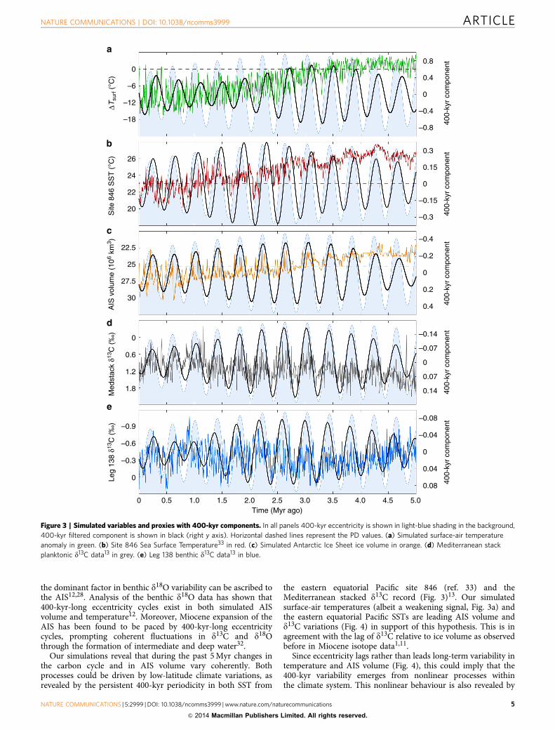
Our simulations reveal that during the past 5 Myr changes inthe carbon cycle and in AIS volume vary coherently. Bothprocesses could be driven by low-latitude climate variations, asrevealed by the persistent 400-kyr periodicity in both SST from

the eastern equatorial Pacific site 846 (ref. 33) and theMediterranean stacked d13C record (Fig. 3)13. Our simulatedsurface-air temperatures (albeit a weakening signal, Fig. 3a) andthe eastern equatorial Pacific SSTs are leading AIS volume andd13C variations (Fig. 4) in support of this hypothesis. This is inagreement with the lag of d13C relative to ice volume as observedbefore in Miocene isotope data1,11.

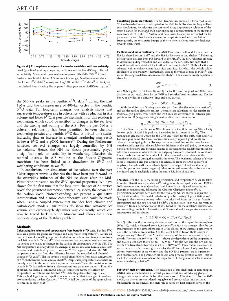
Since eccentricity lags rather than leads long-term variability intemperature and AIS volume (Fig. 4), this could imply that the400-kyr variability emerges from nonlinear processes withinthe climate system. This nonlinear behaviour is also revealed by

0

0

0.4

0.8

–0.8

–0.4

400-

kyr

com

pone

nt40

0-ky

r co

mpo

nent

400-

kyr

com

pone

nt40

0-ky

r co

mpo

nent

400-

kyr

com

pone

nt

–6

ΔTsu

rf (

°C)

Site

846

SS

T (

°C)

AIS

vol

ume

(106

km3 )

–12

–18

26

24

22

20

30

1.8

1.2

0.6

0

0

–0.3

–0.6

–0.9

Med

stac

k δ13

C (

‰)

Leg

138

δ13C

(‰

)

25

22.5

27.5

0.3

0.15

–0.15

–0.3

0.4

0.14

0.08

5.04.54.03.53.02.5Time (Myr ago)

2.01.51.00.50

0.04

–0.04

–0.08

0

0.07

–0.07

–0.14

0

0.2

–0.2

–0.4

0

0

Figure 3 | Simulated variables and proxies with 400-kyr components. In all panels 400-kyr eccentricity is shown in light-blue shading in the background,

400-kyr filtered component is shown in black (right y axis). Horizontal dashed lines represent the PD values. (a) Simulated surface-air temperature

anomaly in green. (b) Site 846 Sea Surface Temperature33 in red. (c) Simulated Antarctic Ice Sheet ice volume in orange. (d) Mediterranean stack

planktonic d13C data13 in grey. (e) Leg 138 benthic d13C data13 in blue.

NATURE COMMUNICATIONS | DOI: 10.1038/ncomms3999 ARTICLE

NATURE COMMUNICATIONS | 5:2999 | DOI: 10.1038/ncomms3999 | www.nature.com/naturecommunications 5

& 2014 Macmillan Publishers Limited. All rights reserved.

the 500-kyr peaks in the benthic d13C data13 during the past1 Myr and the disappearance of 400-kyr cycles in the benthicd18O data. For long-term changes, our analysis shows thatsurface-air temperatures rise in coherence with a reduction in AISvolume and lower d13C. A possible mechanism for this relation isweathering, which could be ascribed to changes in the sea leveland the waxing and waning of the AIS1. For the past 5 Myr, acoherent relationship has been identified between chemicalweathering proxies and benthic d13C data at orbital time scales,indicating that an increase in chemical weathering may resultin lower d13C and a pCO2 increase34. During the Pleistocene,however, sea-level changes are largely controlled by NHice volume. Hence, the NH ice sheets presumably playeda significant role on variability in weathering. Likewise, themarked increase in AIS volume at the Eocene–Oligocenetransition has been linked to a drawdown in d13C andweathering conditions as well35.

In conclusion, our simulations of ice volume over the past5 Myr support previous theories that have been put forward onthe overriding influence of the NH ice sheets after the Mid-Pleistocene transition on the d13C spectral properties. We haveshown for the first time that the long-term changes of Antarcticareveal the persistent interaction between ice sheets, the ocean andthe carbon cycle. Notwithstanding, we present a qualitativeinterpretation and a more comprehensive case could be madewhen using a coupled system that includes both climate andcarbon-cycle models. Our results do show that Antarctic icevolume and carbon-cycle dynamics vary coherently, which cannow be traced back into the Miocene and allows for a newunderstanding of the ‘400-kyr problem’.

MethodsCalculating ice volume and temperature from benthic d18O data. Benthic d18Odata are a proxy for global ice volume and deep-water temperature15. We use aninverse forward modelling approach to deduce ice volume and temperature fromthe LR04 benthic d18O record16. Here we assume that deep-water temperatures andice volume are related to changes in the surface-air temperature over the NH. TheNH temperature anomaly drives the changes in ice volume over Eurasia and NorthAmerica and controls deep-water formation36. The approach derives the NHtemperature anomaly from the difference between the modelled and observedbenthic d18O data17. The ice-volume contribution follows from mass conservationof d18O between the ocean and ice sheets17. Deep-water temperature anomalies arelinearly related to the surface-air temperature anomaly36 and the contribution tobenthic d18O data follows from a palaeotemperature parameterization37. From thisapproach, we derive a continuous and self-consistent record of surface-airtemperature, ice volume and benthic d18O data (Supplementary Fig. S1a–c).This methodology has been applied in several studies that investigate ice-volumeevolution during the late Cenozoic17,20,28,36. A full description of the approach canbe read in de Boer et al.17

Simulating global ice volume. The NH temperature anomaly is forwarded to four3D ice-sheet-shelf models and applied to the SMB fields. To allow for long million-year simulations, ice velocities are computed using approximate solutions of thestress balance for sheet and shelf flow, including a representation of the transitionzone from sheet to shelf17. Surface and basal mass balance are accounted for byparameterizations that include changes in temperature and solar insolation.Subsequently, the total mass budget of the ice sheet is closed with ice dischargetowards open water.

Ice fluxes and mass continuity. The ANICE ice-sheet-shelf model is based on theSIA for sheet flow on land38 and the SSA for ice streams and shelves39. Followingthe approach that has been put forward in the PISM40, the SSA velocities are usedto determine sliding velocities and are added to the SIA velocities such that asmooth transition is obtained for ice-flow from sheet to shelf41. Both velocities areadjusted with an enhancement factor ESIA and ESSA, for which the default valuesare chosen to be 5.0 and 0.7, respectively, close to the values as used in PISM25, andwithin the range as determined in a recent study24. The mass continuity equation isgiven by:

@Hi@t¼ r! � QþB; ð1Þ

with Hi being the ice thickness (in m), Q the ice flux (m2 per year) and B the massbalance (m per year), given by the SMB and sub-shelf melt or refreezing. The iceflux Q is divided in a diffusive (SIA) and SSA part as:

Q ¼ �Dr!Hsþ V!

SSAHi: ð2ÞWith the diffusivity D being the scalar part from the SIA velocity equation17,

and Hs the surface elevation (in m). Velocities are calculated on the regular icethickness grid points, from which the ice fluxes are determined in between gridpoints A and B (staggered) using a centred difference discretization:

Q ¼ ðDA þDBÞ2

ðHsA þHsBÞ2

þ VA þVB

2Hi: ð3Þ

In the SSA term, ice thickness Hi is chosen to be HiA if the average SSA velocitybetween point A and B is positive, if negative, Hi is chosen to be HiB. Therectangular grid size is 20 km for the GrIS and 40 km for the EuIS, NaIS and AIS.For each grid point, the fluxes towards the directly adjacent grid points arecalculated as outgoing fluxes. To keep mass conserved, in case the mass balance isnegative and larger than the available ice thickness at the grid point, the outgoingfluxes are set to zero and the mass balance is set equal to the available ice thickness.After the mass conservation check, the outgoing fluxes are reduced if the combinedflux exceeds the sum of the available ice thickness and mass balance (eithernegative or positive) during that specific time step. The total mass balance of the icesheet is conserved and per definition is calculated from the SMB (positive ornegative), the sub-shelf mass balance (positive or negative) and ice dischargetowards open ocean points (negative). Mass conservation over the entire domain ismonitored and is negligible during the entire 5.32 Myr simulation.

The SMB. For the SMB, the initial precipitation and temperature fields are takenfrom the ERA-40 Reanalysis data set42, using monthly averaged fields from 1971 to2000. Accumulation over Greenland and Antarctica is adjusted according tochanges in temperature, following the Clausius–Clapeyron relation17. Aprecipitation model has been used for the two large NH ice sheets to adjust the PDprecipitation fields. The model includes orographic forcing of precipitation andchanges in the moisture content, which are calculated from the 2-m surface-airtemperature and the 850-hPa wind fields17. The melt rate (in m w.e. per year) iscalculated from a parameterization that is based on PD mass balance observationsand modelling results for Antarctica and Greenland and incorporates changes intemperature and insolation:

A ¼ Dtð0:513ð1� aÞQþ 10Ts þCablÞ=ðrfwLÞ; ð4Þhere Q is the monthly incoming shortwave radiation at the top of the atmosphere(W m� 2), which is changed every 1,000 years43, 0.513 is an average value for thetransmissivity of the atmosphere and a is the albedo of the surface. Furthermore,rfw is the density of fresh water, L is the latent heat of fusion (both shown inSupplementary Table S3) and Dt is the time step of the melt model—that is, amonth. The constant 10 (W m� 2 K� 1) shows the dependence on the temperature,and Cabl is a constant that is set to � 32 W m� 2 for the AIS and the two NH icesheets. For Greenland, this value is set to � 40 W m� 2. These values are chosen insuch a way that after several glacial cycles the PD ice volume closely matches thecurrent observations of ice volume, and the PD SMB patterns are in agreementwith observations. The parameterization can only produce positive values—that is,melt of ice—and also accounts for the importance of changes in the solar insolationwhen calculating ablation44.

Sub-shelf melt or refreezing. The calculation of sub-shelf melt or refreezing inANICE uses a combination of several parameterizations introducing glacial–interglacial changes and ice shelves that show close to PD extent22,25. For the GrISmodel, ice shelves are considered negligible and are not taken into account.Underneath the ice shelves, the melt rate is based on heat transfer between the

150

50

–50

–100

–150

0.25 1.250.75 1.75 2.25Time (Myr ago)

2.75 3.25 3.75 4.25 4.75

Lead

w.r.

t. ec

cent

ricity

(ky

r)

0

100

Figure 4 | Cross-phase analysis of climate variables with eccentricity.

Lead (positive) and lag (negative) with respect to the 400-kyr filter of

eccentricity. Surface-air temperature in green, Site 846 SSTs33 in red,

Eustatic sea level in blue, AIS volume in orange, Mediterranean stack

planktonic d13C data13 in grey and Leg 138 benthic d13C data13 in black, with

the dashed line showing the apparent disappearance of 400-kyr cycles13.

ARTICLE NATURE COMMUNICATIONS | DOI: 10.1038/ncomms3999

6 NATURE COMMUNICATIONS | 5:2999 | DOI: 10.1038/ncomms3999 | www.nature.com/naturecommunications

& 2014 Macmillan Publishers Limited. All rights reserved.

bottom of the ice and the ocean water25,45:

Smelt ¼ rwcpOgTFmeltðToc �Tf Þ=Lri; ð5Þ

with the different parameters adopted from PISM25 and shown in SupplementaryTable S3. Here rw is the seawater density (kg m� 3), cpO is the specific heat capacityof the ocean (J kg� 1 �C� 1), gT is the thermal exchange velocity (m s� 1), Fmelt thesub ice-shelf melt parameter (m s� 1), L the Latent heat of fusion (J kg� 1) and ri

the density of ice. Toc is the ocean-water temperature (�C) adjusted with aweighting function (equation (7)). The melt rate can have both positive andnegative values, either leading to melting of ice shelves or (re)freezing of oceanwater45. The freezing temperature of the saline ocean water (in �C) at the shelf baseis calculated with:

Tf ¼ 0:0939� 0:057 � SO þ 7:64�10� 4zb; ð6Þwith SO¼ 35 psu being the average salinity of the ocean water and zb being thedepth of the ice-shelf base (in m) calculated as: zb¼ � (ri/rw)Hi. To simulateglacial–interglacial climate variability, the ocean temperature Toc in equation (5) isadjusted with a weighting function, including changes in temperature and a smallinfluence of summer insolation22:

wg ¼ 1þDT=12þMaxð0;Dqj=40Þ 2 ½0; 2�: ð7ÞHere DT is the applied temperature anomaly relative to PD. Furthermore, Dqj is

the summer insolation anomaly relative to PD, using the January 80 �S anomaly forthe AIS, and the June 65�N anomaly (W m� 2) for the large NH ice sheets. Theocean temperature is then adjusted for colder than PD periods, when 0rwgo1, as:

Toc ¼ ð1�wgÞTCD þwg TPD; ð8Þ

and for warm periods, when 1rwgr2:

Toc ¼ ð2�wgÞTPD þðwg � 1ÞTWM: ð9ÞTCD, TPD and TWM indicate the cold, PD and warm values of the uniform ocean

temperature as shown in Supplementary Table S3. These values are applied to theice sheets as spatial uniform values and are based on values found in climatemodels and observations46,47.

References1. Palike, H. et al. The heartbeat of the Oligocene climate system. Science 314,

1894–1898 (2006).2. PALEOSENS Project Members. Making sense of palaeoclimate sensitivity.

Nature 491, 683–691 (2012).3. Siegenthaler, U. et al. Stable carbon cycle-climate relationship during the late

Pleistocene. Science 310, 1313–1317 (2005).4. Kohler, P. et al. What caused Earth’s temperature variations during the last

800,000 years? Data-based evidence on radiative forcing and constraints onclimate sensitivity. Quat. Sci. Rev. 29, 129–145 (2010).

5. Naish, T. et al. Obliquity-paced Pliocene West Antarctic ice sheet oscillations.Nature 458, 322–328 (2009).

6. Huybers, P. Combined obliquity and precession pacing of late Pleistocenedeglaciations. Nature 480, 229–232 (2011).

7. Sigman, D. M., Hain, M. P. & Haug, G. H. The polar ocean and glacial cycles inatmospheric CO2 concentration. Nature 466, 47–55 (2010).

8. Coxall, H., Wilson, P., Palike, H., Lear, C. & Backman, J. Rapid stepwise onsetof Antarctic glaciation and deeper calcite compensation in the Pacific Ocean.Nature 433, 53–57 (2005).

9. DeConto, R. M. & Pollard, D. Rapid Cenozoic glaciation of Antarctica triggeredby declining atmospheric CO2. Nature 421, 245–249 (2003).

10. Zachos, J. C., Shackleton, N. J., Revenaugh, J. S., Palike, H. & Flower, B. P.Climate response to orbital forcing across the Oligocene-Miocene boundary.Science 292, 274–278 (2001).

11. Holbourn, A., Kuhnt, W., Schulz, M., Flores, J.-A. & Andersen, N. Orbitally-paced climate evolution during the middle Miocene ‘Monterey’ carbon-isotopeexcursion. Earth Planet. Sci. Lett. 261, 534–550 (2007).

12. Liebrand, D. et al. Antarctic ice sheet and oceanographic response toeccentricity forcing during the early Miocene. Clim. Past 7, 869–880 (2011).

13. Wang, P., Tian, J. & Lourens, L. J. Obscuring of long eccentricity cyclicity inPleistocene oceanic carbon isotope records. Earth Planet. Sci. Lett. 290,319–330 (2010).

14. Imbrie, J. & Imbrie, J. Modeling the climatic response to orbital variations.Science 207, 943–953 (1980).

15. Chappell, L. & Shackleton, N. J. Oxygen isotopes and sea level. Nature 324,137–140 (1986).

16. Lisiecki, L. & Raymo, M. A Pliocene stack of 57 globally distributed benthicd18O records. Paleoceanography 20, PA1003 (2005).

17. de Boer, B., van de Wal, R. S. W., Lourens, L. J. & Bintanja, R. A continuoussimulation of global ice volume over the past 1 million years with 3-D ice-sheetmodels. Clym. Dyn. 41, 1365–1384 (2013).

18. Meyers, S. R. & Hinnov, L. A. Northern hemisphere glaciation and theevolution of Plio-Pleistocene climate noise. Paleoceanography 25, PA3207(2010).

19. Lourens, L. J. et al. Linear and non-linear response of late Neogene glacial cyclesto obliquity forcing and implications for the Milankovitch theory. Quat. Sci.Rev. 29, 352–365 (2010).

20. Bintanja, R. & Van de Wal, R. S. W. North American ice-sheet dynamics andthe onset of 100,000-year glacial cycles. Nature 454, 869–872 (2008).

21. Clark, P. U. et al. The middle Pleistocene transition: characteristics,mechanisms, and implications for long-term changes in atmospheric pCO2.Quat. Sci. Rev. 25, 3150–3184 (2006).

22. Pollard, D. & DeConto, R. M. Modelling West Antarctic ice sheet growth andcollapse through the past five million years. Nature 458, 329–332 (2009).

23. DeConto, R. M., Pollard, D. & Kowalewski, D. Modeling Antarctic ice sheet andclimate variations during marine isotope stage 31. Glob. Planet. Change 88–89,45–52 (2012).

24. Ma, Y. et al. Enhancement factors for grounded ice and ice shelves inferredfrom an anisotropic ice-flow model. J. Glaciol. 56, 805–812 (2010).

25. Martin, M. A. et al. The Potsdam Parallel Ice Sheet Model (PISM-PIK) –Part 2:Dynamic equilibrium simulation of the Antarctic ice sheet. Cryosphere 5,727–740 (2011).

26. Robinson, A., Calov, R. & Ganopolski, A. Greenland ice sheet modelparameters constrained using simulations of the Eemian Interglacial. Clim. Past7, 381–396 (2011).

27. de Boer, B., van de Wal, R., Bintanja, R., Lourens, L. & Tuenter, E. Cenozoicglobal ice-volume and temperature simulations with 1-D ice-sheet modelsforced by benthic d18O records. Ann. Glaciol. 51, 23–33 (2010).

28. de Boer, B., van de Wal, R. S. W., Lourens, L. J. & Bintanja, R. Transientnature of the Earth’s climate and the implications for the interpretation ofbenthic d18O records. Palaeogeogr. Palaeoclimatol. Palaeoecol. 335–336, 4–11(2012).

29. Elderfield, H. et al. Evolution of ocean temperature and ice volume through theMid-Pleistocene climate transition. Science 337, 704–709 (2012).

30. Ruddiman, W. F. Orbital changes and climate. Quat. Sci. Rev. 25, 3092–3112(2006).

31. Pritchard, H. D. et al. Antarctic ice-sheet loss driven by basal melting of iceshelves. Nature 484, 502–505 (2012).

32. Holbourn, A., Kuhnt, W., Frank, M. & Haley, B. A. Changes in Pacific Oceancirculation following the Miocene onset of permanent Antarctic ice cover. EarthPlanet. Sci. Lett. 365, 38–50 (2013).

33. Herbert, T., Peterson, L., Lawrence, K. & Liu., Z. Tropical ocean temperaturesover the past 3.5 Myr. Science 328, 1530–1534 (2010).

34. Tian, J., Xie, X., Ma, W., Jin, H. & Wang, P. X-ray fluorescence core scanningrecords of chemical weathering and monsoon evolution over the past 5 Myr inthe southern South China Sea. Paleoceanography 26, PA4202 (2011).

35. Merico, A., Tyrrell, T. & Wilson, P. A. Eocene/Oligocene ocean de-acidificationlinked to Antarctic glaciation by sea-level fall. Nature 452, 979–982 (2008).

36. Bintanja, R., Van de Wal, R. S. W. & Oerlemans, J. Modelled atmospherictemperatures and global sea level over the past million years. Nature 437,125–128 (2005).

37. Duplessy, J.-C., Labeyrie, L. & Waelbroeck, C. Constraints on the oceanoxygen isotopic enrichment between the Last Glacial Maximum andthe Holocene: Paleoceanographic implications. Quat. Sci. Rev. 21, 315–330(2002).

38. Hutter, L. Theoretical Glaciology (D. Reidel, Dordrecht, 1983).39. Morland, L. W. Unconfined ice-shelf flow. in Dynamics of the West Antarctic

Ice Sheet (eds de Veen, C. J. V. & Oerlemans, J.) 99–116 (D. Reidel, 1987).40. Winkelmann, R. et al. The Potsdam Parallel Ice Sheet Model (PISM-PIK) –Part

1: Model description. Cryosphere 5, 715–726 (2011).41. Bueler, E. & Brown, J. Shallow shelf approximation as a ‘sliding law’ in a

thermomechanically coupled ice sheet model. J. Geophys. Res. 114, F03008(2009).

42. Uppala, S. M. et al. The ERA-40 re-analysis. Q. J. R. Meteorol. Soc. 131,2961–3012 (2005).

43. Laskar, J. et al. A long-term numerical solution for the insolation quantities ofthe Earth. Astron. Astrophys. 428, 261–285 (2004).

44. van de Berg, W. J., van den Broeke, M., Ettema, J., van Meijgaard, E. &Kaspar, F. Significant contribution of insolation to Eemian melting of theGreenland ice sheet. Nat. Geosci. 4, 679–683 (2011).

45. Beckmann, A. & Goosse, H. A parameterization of ice shelf-ocean interactionfor climate models. Ocean Model. 5, 157–170 (2003).

46. Braconnot, P. et al. Results of PMIP2 coupled simulations of the Mid-Holoceneand Last Glacial Maximum - Part 1: experiments and large-scale features. Clim.Past 3, 261–277 (2007).

47. Dowsett, H. J. et al. The PRISM3D paleoenvironmental reconstruction.Stratigraphy 7, 123–139 (2010).

48. Grinsted, A., Moore, J. C. & Jevrejeva, S. Application of the cross wavelettransform and wavelet coherence to geophysical time series. Nonlin. ProcessesGeophys. 11, 561–566 (2004).

49. Paillard, D., Labeyrie, L. & Yiou, P. Macintosh program performs time-seriesanalysis. Eos Trans. AGU 77, 379 (1996).

NATURE COMMUNICATIONS | DOI: 10.1038/ncomms3999 ARTICLE

NATURE COMMUNICATIONS | 5:2999 | DOI: 10.1038/ncomms3999 | www.nature.com/naturecommunications 7

& 2014 Macmillan Publishers Limited. All rights reserved.

AcknowledgementsThis research was funded through the KNAW professorship of Johannes Oerlemans.Model runs were performed on the LISA Computer Cluster. We would like to thankSurfSARA Computing and Networking Services for their support.

Author contributionsB.d.B. performed the experiments, the analysis and wrote the manuscript. All authorscontributed to the discussion of the results and implications and commented on themanuscript at all stages.

Additional informationSupplementary Information accompanies this paper at http://www.nature.com/naturecommunications

Competing financial interests: The authors declare no competing financial interests.

Reprints and permission information is available online at http://npg.nature.com/reprintsandpermissions/

How to cite this article: de Boer, B. et al. Persistent 400,000-year variability of Antarcticice volume and the carbon cycle is revealed throughout the Plio-Pleistocene. Nat.Commun. 5:2999 doi: 10.1038/ncomms3999 (2014).

ARTICLE NATURE COMMUNICATIONS | DOI: 10.1038/ncomms3999

8 NATURE COMMUNICATIONS | 5:2999 | DOI: 10.1038/ncomms3999 | www.nature.com/naturecommunications

& 2014 Macmillan Publishers Limited. All rights reserved.