Permutation orbifolds of supersymmetric minimal models

arX

iv:1

011.

0934

v1 [

hep-

th]

3 N

ov 2

010

Permutation orbifolds of N = 2supersymmetric minimal models

M. Maio1 and A.N. Schellekens1,2,3

1Nikhef Theory Group, Amsterdam, The Netherlands

2IMAPP, Radboud Universiteit Nijmegen, The Netherlands

3Instituto de Fısica Fundamental, CSIC, Madrid, Spain

November 4, 2010

Abstract

In this paper we apply the previously derived formalism of per-mutation orbifold conformal field theories to N = 2 supersymmetricminimal models. By interchanging extensions and permutations of thefactors we find a very interesting structure relating various conformalfield theories that seems not to be known in literature. Moreover, un-expected exceptional simple currents arise in the extended permutedmodels, coming from off-diagonal fields. In a few situations they admitfixed points that must be resolved. We determine the complete CFTdata with all fixed point resolution matrices for all simple currents ofall Z2-permutations orbifolds of all minimal N = 2 models with k 6= 2mod 4.

NIKHEF/2010-37

1

Contents

1 Introduction 2

1.1 Basic concepts . . . . . . . . . . . . . . . . . . . . . . . . . . . 51.2 Plan . . . . . . . . . . . . . . . . . . . . . . . . . . . . . . . . 8

2 N = 2 minimal models 9

2.1 The N = 2 SCFT and minimal models . . . . . . . . . . . . . 92.2 Parafermions . . . . . . . . . . . . . . . . . . . . . . . . . . . 112.3 String functions and N = 2 Characters . . . . . . . . . . . . . 122.4 Modular transformations and fusion rules . . . . . . . . . . . . 15

3 Permutation orbifold 15

4 Permutations of N = 2 minimal models 18

4.1 Extension by (TF , 1) . . . . . . . . . . . . . . . . . . . . . . . 214.2 Extension by (TF , 0) . . . . . . . . . . . . . . . . . . . . . . . 244.3 Common properties . . . . . . . . . . . . . . . . . . . . . . . . 26

5 Exceptional simple currents and their fixed points 27

5.1 k = 2 Example . . . . . . . . . . . . . . . . . . . . . . . . . . 32

6 Orbit structure for N = 2 and N = 1 34

7 Conclusion 37

A Twisted-fields orbits of the (0, 1)-current 39

B Fusion rules of 〈0, TF 〉 and corresponding split fields 40

B.1 Before (TF , ψ)-extension . . . . . . . . . . . . . . . . . . . . . 41B.2 After (TF , ψ)-extension . . . . . . . . . . . . . . . . . . . . . . 42

1 Introduction

Rational conformal field theory (RCFT) [1] has proved to be a useful toolfor studying perturbative string theory, and especially string model build-ing. It provides a middle ground between approaches based on free fieldtheories (free bosons, free fermions and orbifolds) on the one hand and geo-metric constructions on the other hand. While free field theory constructionsare undoubtedly simpler and more easily applicable to the computation offeatures of phenomenological interest such as couplings and moduli depen-dence, there is a danger of them being too special. This may lead to incorrect

2

conclusions about what is possible or not in string theory, and how genericcertain features are. For example, the earliest attempts to obtaining MSSMspectra using orbifold-based orientifolds were plagued by chiral exotics [2].However, the first detailed exploration of interacting RCFT orientifolds pro-duced hundreds of thousands of distinct spectra without such unacceptableparticles [3].

However, the set of RCFTs at our disposal is disappointingly small.Decades ago it was conjectured that the moduli spaces of string theory weredensely populated by RCFT points, just as the c = 1 moduli space is denselypopulated by rational circle compactifications and their orbifolds. Even to-day, it is not clear what the status of that conjecture is, but it certainlydoes not have any practical value. The only interacting RCFTs that we canreally use for building exact string are tensor products of N = 2 minimalmodels, also known as “Gepner models” [5, 6]. Indeed, these are the onlyones that have been used in orientifold model building. In this situation weface the same risk mentioned above regarding free CFTs: perhaps what weare finding is too special. For example, in a study of the number of familiesin Gepner orientifolds it was found that the number three was suppressed bya disturbing two to three orders of magnitude [3] (similar conclusions wereobtained for Z2 × Z2 orientifolds in [4]). The origin of this phenomenon is,to our knowledge, still not understood, but it would be interesting to knowif it persists beyond Gepner models.

The other area of application of RCFT model building, and the one whereit was historically used first, is the heterotic string. In this case a few resultsare available beyond Gepner model building. This is possible because thecomputation of the simplest heterotic spectra requires slightly less CFT datathan what is needed for orientifold spectra.

The full power of RCFT model building only manifests itself if one usesthe complete set [7] of simple current modular invariant partition functions(MIPFs) [8, 9] (See [11] for a review of simple current MIPFs. The underlyingsymmetries were discovered independently in [10]). Indeed, with only thetrivial (diagonal or charge conjugation) MIPFs essentially nothing wouldhave been found in orientifold model building. Indeed, already basic physicalconstraints like world-sheet and space-time supersymmetry require a simplecurrent MIPF. Although the simple current symmetries can be read off fromthe modular transformation matrix S, and the corresponding MIPFs canbe readily constructed, often additional information is required when thesimple current action has fixed points [12, 11]. In order to make full useof the complete simple current formalism we need the following data of theCFT under consideration:

3

• The exact conformal weights.

• The exact ground state dimensions.

• The modular transformation matrix S.

• The fixed point resolution matrices SJ , for simple currents J with fixedpoints.

Not all of this information is needed in all cases. The matrices S and SJ areneeded in the computation of boundary coefficients of orientifolds for simplecurrent MIPFs. In heterotic spectrum computations all we need to know isthe first two items, plus the simple current orbits implied by S. To computethe Hodge numbers of heterotic compactifications, we only need to know theexact ground state dimensions of the Ramond ground states.

In addition to Gepner models, for which all this information is available,there are at least two other classes that are potentially usable: the Kazama-Suzuki models [13] and the permutation orbifolds. In the former case, thecoset construction gives us the exact matrix S, and the results of [14] pro-vide all the matrices SJ . The difficulty lies in computing the exact CFTspectrum and the ground state dimensions. In some cases this just requiresthe computation of branching functions, a tedious task that can however beperformed systematically. To our knowledge this has never been done, how-ever. In other cases, those with field identification fixed points, no algorithmis currently available. In both cases, it has been possible to compute at leastthe Hodge numbers for the diagonal MIPF (see respectively [15] and [16]),although in the latter case this required some rather involved tricks to dealwith fixed point resolution.

For permutation orbifolds the situation is more or less just the other wayaround: it has been known for a long time how to compute their weightsand ground state dimensions, but there was no formalism for computing Sand SJ . Also in this case it has been possible to compute the Hodge num-bers and even the number of singlets for the diagonal invariants [17, 18].However, meanwhile it as become clear that the values of Hodge numbersoffer a rather poor road map to the heterotic string landscape. In par-ticular they lead to the wrong impression that the number of families islarge and very often a multiple of 4 or 6. The former problem disappearsif one allows breaking of the gauge group E6 to phenomenologically moreattractive subgroups (ranging from SO(10) via SU(5) or Pati-Salam to justSU(3)× SU(2)× U(1) (times other factors) by allowing asymmetric simplecurrent invariants [19, 20], whereas the second problem can be solved bymodifying the bosonic sector of the heterotic string, for example by means

4

of heterotic weight lifting [21], B-L lifting [22] or E8 breaking [23]. All ofthese methods require knowledge of the full simple current structure of thebuilding blocks. This in its turn requires knowing S.

A first step towards the computation of S for Z2 permutation orbifoldswas made in [24], almost ten years after permutation orbifolds were first stud-ied. While this might seem sufficient for permutation orbifolds in heteroticstring model building, we will see that even in that case more is needed. Fororientifold model building with general simple current MIPFs certainly moreis needed, as already mentioned above. The crucial ingredient in both casesis fixed point resolution. Therefore we expect that significant progress canbe made by applying results we obtained recently [25, 26, 27], extending theresults of [24] to fixed point resolution matrices SJ , for currents J of order2. Since in N = 2 minimal models all currents with fixed points have order2, this seems to be precisely what is needed. The purpose of this paper isto determine which of the CFT data listed above can now be computed forpermutations orbifolds of N = 2 minimal models, and provide algorithms fordoing so.

1.1 Basic concepts

The easiest way of constructing rational conformal field theories is by takingthe tensor product of existing ones. In the resulting CFT, all relevant CFTdata is known from its factor theories. Another possibility is to take orbifolds.Orbifolds are already non-trivial theories, since they admit an untwisted anda twisted sector. The twisted sector is demanded by modular invariance.Normally the untwisted sector is easily derivable from the original theory,but twisted fields are much harder to determine.

There are many kind of orbifolds, depending on the particular modelunder consideration. In this paper we will consider the permutation orbifold,which arises when a tensor product CFT has at least two identical factorthat can be permuted. The simplest instance of this orbifold is when thereare only two identical factors to interchange. Start with the CFT A andbuild the tensor product A⊗A. It has a manifest Z2 symmetry which flipsthe two factors. We denote this Z2 orbifold as

A⊗A/Z2 . (1.1)

The spectrum was worked out for the first time in [17] using modular invari-ance, and twisted fields were determined. Subsequently, the modular S andT matrices were given in [24] using an induction procedure on the algebragenerators.

5

The next level of complication for a CFT is the simple-current extension.A simple current is a particular field of the theory, with simple fusion ruleswith any other field. If they have integer spin, they can be used to write downnew modular invariant conformal field theories, known as simple currentinvariants. In the extension procedure, one computes the monodromy chargeQJ of each field with respect to the simple current J and organizes fieldsinto orbits, keeping only those with integer monodromy. Algebraically, anextension is an orbifold projection, where one keeps states which are invariantunder the monodromy operator e2iπQJ and adds the twisted sector.

In principle the CFT data of such invariants are determined by those ofthe original theory, but the level of difficulty rapidly increases if there arefixed points, i.e. fields that the simple current leaves fixed under the fusionrules. Equivalently, fixed points are orbits with length one. If there are fixedpoints one needs a set of matrices “SJ” for each current J acting on the fixedpoints [28]. Outside the fixed points of J , SJ vanishes. The full modular Smatrix is then expressed in terms of these SJ matrices in a complicated way.Expressions for the SJ matrix are known for WZW models, coset theoriesand extensions thereof [12, 28, 29, 30].

When we combine extensions and permutation orbifolds, things becomemuch more interesting and complicated at the same time. There it is alwaysneeded to worry about fixed point resolutions and SJ matrices. The structureof simple currents and fixed points in the permutation orbifold was derived in[25, 26] and also a unitary and modular invariant ansatz for the SJ matricesexists [27]. Using the formula of [28], we have checked that in simple currentextensions these matrices SJ yield a good S matrix (satisfying the condition(ST )3 = S2) and produce non-negative integer coefficients in the fusion rules.

One may distinguish five kinds of fields in permutation orbifolds, whichwe will denote as follows. The labels i and j refer to primaries of the originalCFT1:

• Diagonal fields (i, ξ), with ξ = 0 or 1. Here ξ = 0 labels the symmetriccombination and ξ = 1 the anti-symmetric one.

• Off-diagonal fields 〈i, j〉, i < j.

• Twisted fields (i, ξ), with ξ = 0 or 1. The (i, 1) denotes the excitedtwist field.

1We use a different notation for off-diagonal combinations than previous work [24, 25,26, 27]: 〈i, j〉 instead of (i, j). This is to prevent confusion between the antisymmetriccombination of the vacuum module, (0, 1), and the off-diagonal combination of fields nr.0 and 1. The comma will be omitted in some cases.

6

Exact formulas for the Virasoro characters of all these representations areknown [24], and can be used to get the exact ground state conformal weightand dimensions (see chapter 3 for further details).

Here we want to apply the results of [24] and [25, 26, 27] to N = 2minimal models. This may seem to be straightforward, as a supersymmet-ric CFT is just an example of a CFT, and the aforementioned results holdfor any CFT. However, the permutation orbifold obtained by applying [24]turns out not to have world-sheet supersymmetry. This is related to the factthat a straightforward Virasoro tensor product (the starting point for thepermutation orbifold) does not have world-sheet supersymmetry either, forthe simple reason that tensoring produces combinations of R and NS fields.The solution to this problem in the case of the tensor product is to extendthe chiral algebra by a simple current of spin 3, the product of the world-sheet supercurrents of the two factors (or any two factors if there are morethan two). One might call this the supersymmetric tensor product. But forthis extended tensor product the formalism of [24] is not available. One canfollow two paths to solve that problem: either one can try to generalize [24]to supersymmetric tensor products (or more generally to extended tensorproducts) or one can try to supersymmetrize the permutation orbifold. Wewill follow the second path.

One might expect that the chiral algebra of permutation orbifold hasto be extended in order to restore world-sheet supersymmetry. That is in-deed correct, but it turns out that there are two plausible candidates forthis extension: the symmetric and the anti-symmetric combination of theworld-sheet supercurrent of the minimal model. Denoting the latter as TF ,the two candidates are the spin-3 currents (TF , 0) and (TF , 1). Somewhatcounter-intuitively, it is the second one that leads to a CFT with world-sheetsupersymmetry. The first one, (TF , 0), gives rise to a CFT that is similar,but does not have a spin-3/2 current of order 2.

Both (TF , 0) and (TF , 1) have fixed points, but we know their resolutionmatrices from the general results of [27]. They come in handy, becauseit turns out that one of these fixed points is the off-diagonal field 〈0, TF 〉of conformal weight 3

2. As stated above, this is not a simple current of

the permutation orbifold, but it is a well-known fact that chiral algebraextensions can turn primaries into simple currents. This is indeed preciselywhat happens here. Since we know the fixed point resolution matrices of(TF , 0) and (TF , 1) we can work out the orbits of this new simple current.It turns out that in the former extension 〈0, TF 〉 has order 4, whereas in thelatter it has order 2. We conclude that the latter must be the supersymmetricpermutation orbifold; we will refer to this CFT as “X”. The fixed pointresolution also determines the action of the new world-sheet supercurrent

7

〈0, TF 〉 on all other fields, combining them into world-sheet superfields ofeither NS or R type.

The current 〈0, TF 〉 has no fixed points, as one would expect in an N = 2CFT (because it has two supercurrents of opposite charge, and acting witheither one changes the charge). However, there are in general more off-diagonal fields that turn into simple currents. Some of these do have fixedpoints, and since the simple currents originate from fields that were notsimple currents in the permutation orbifold, our previous results do not allowus to resolve these fixed points. We find that this problem only occurs ifk = 2 mod 4, where k = 1 . . .∞ is the integer parameter labelling theN = 2 minimal models.

To prevent confusion we list here all the CFTs that play a role in thestory:

• The N = 2 minimal models.

• The tensor product of two identical N = 2 minimal models. We willrefer to this as (N = 2)2.

• The BHS-orbifold of the above. This is the permutation orbifold asdescribed in [24]. It will be denoted (N = 2)2orb.

• The supersymmetric extension of the tensor product. This is the ex-tension of the tensor product by the spin-3 current (TF , TF ). We willcall this CFT (N = 2)2Susy

• The supersymmetric permutation orbifold (N = 2)2Susy−orb. This isBHS orbifold extended by the spin-3 current (TF , 1)

• The non-supersymmetric permutation orbifoldX . This is BHS orbifoldextended by the spin-3 current (TF , 0)

1.2 Plan

The plan of this paper is as follows.in section 2 we review the theory of N = 2 minimal models, their spectrumand S matrix. As far as the characters are concerned, we recall the cosetconstruction and state a few known results from parafermionic theories, inparticular the string functions.In section 3 we review general permutation orbifolds, the BHS formalism andits generalization to fixed point resolution matrices. Then in section 4 wemove to the permutation orbifold of N = 2 minimal models. We consider

8

extensions by the various currents related to the spin-32worldsheet supercur-

rent and explain how the exceptional off-diagonal currents appear. We alsowork out the special extension of the orbifold by the symmetric and anti-symmetric representation of the worldsheet current.In section 5 we study we study the exceptional simple currents and in par-ticular the ones that have got fixed points. We give the structure of theseoff-diagonal currents as well as of their fixed points, in the case they haveany. We illustrate the general ideas with the example of the minimal model atlevel two. In section 6 we summarize the orbit and fixed point structures forthe various CFTs we consider, and we also present the analogous results forN = 1 minimal models, where similar issues arise, and also some interestingdifferences. in section 7 we give our conclusions.

2 N = 2 minimal models

In this section we review the minimal model of the N = 2 super conformalalgebra.

2.1 The N = 2 SCFT and minimal models

The N = 2 super conformal algebra (SCA) was first introduced in [33]. Itcontains the stress-energy tensor T (z) (spin 2), a U(1) current j(z) (spin1) and two fermionic currents T±

F (z) (spin 32). In operator product form it

reads:

T (z)T (0) ∼ c

2z4+

2

z2T (0) +

1

z∂T (0) (2.1a)

T (z)T±F (0) ∼ 3

2z2T±F (0) +

1

z∂T±

F (0) (2.1b)

T (z)j(0) ∼ 1

z2j(0)

1

z∂j(0) (2.1c)

T+F (z)T

−F (0) ∼ 2c

3z3+

2

z2j(0) +

2

zT (0) +

1

z∂j(0) (2.1d)

T+F (z)T

+F (0) ∼ T−

F (z)T−F (0) ∼ 0 (2.1e)

j(z)T±F (0) ∼ ±1

zT±F (0) (2.1f)

j(z)j(0) ∼ c

3z2. (2.1g)

Using the mode expansion

T (z) =∑

n∈Z

Lnzn+2

, j(z) =∑

n∈Z

Jnzn+1

, T±F (z) =

∑

r∈Z±ν

G±r

zr+3

2

, (2.2)

9

the algebra (2.1) is equivalent to the (anti-)commutators

[Lm, Ln] = (m− n)Lm+n +c

12(m3 −m)δm,−n (2.3a)

[Lm, Jn] = −nJm+n , (2.3b)

{G+r , G

−s } = 2Lr+s + (r − s)Jr+s +

c

3(r2 − 1

4)δr,−s (2.3c)

{G+r , G

+s } = {G−

r , G−s } = 0 , (2.3d)

[Jm, G±r ] = ±1

cG±r+n , (2.3e)

[Jm, Jn] =c

3mδm,−n . (2.3f)

The shift ν can in principle be real, but for our considerations we take itto be integer (NS sector) or half-integer (R sector). Unitary representa-tions of the N = 2 SCA can exists for values of the central charge c ≥ 3(infinite-dimensional representations) and for the discrete series c < 3 (finite-dimensional representations). The latter ones are discrete conformal fieldtheories, the N = 2 minimal models, whose central charge is specified by aninteger number k, called the level, according to:

c =3k

k + 2. (2.4)

The Cartan subalgebra is generated by L0 and J0, hence primary fields arelabelled by their weights h and charges q:

L0|h, q〉 = h|h, q〉 , J0|h, q〉 = q|h, q〉 . (2.5)

The allowed values for h and q are given by

hl,m,s =l(l + 2)−m2

4(k + 2)+s2

8, qm,s = − m

k + 2+s2

2, (2.6)

where l, m, s are integer numbers with the property that

• l = 0, 1, . . . , k

• m is defined mod 2(k+2) (we will choose the range −k−1 ≤ m ≤ k+2)

• s = −1, 0, 1, 2 mod 4; s = 0, 2 for NS sector, s = ±1 for R sector.

In addition, in order to avoid double-counting, one has to take into accountthat not all the fields are independent but are rather identified pairwise:

φl,m,s ∼ φk−l,m+k+2,s+2 . (2.7)

10

In order to be able to say something about the characters of the minimalmodel, let us mention the coset construction. The N = 2 minimal modelscan be described in terms of the coset

su(2)k × u(1)2u(1)k+2

. (2.8)

Throughout this paper, we use the convention that u(1)p contains 2p primaryfields. The characters of this coset are decomposed according to

χsu(2)kl (τ) · χu(1)2s (τ) =

k+2∑

m=−k−1

χu(1)k+2

m (τ) · χl,m,s(τ) , (2.9)

where χl,m,s are the characters (branching functions) of the coset theory.

2.2 Parafermions

We will soon see that χl,m,s will be determined in terms of the so-called string

functions, which are related to the characters of the parafermionic theories

[34, 35]. In order to determine χl,m,s, let us consider su(2)k representations.Using the Weyl-Kac character formula [36, 37], su(2)k characters are givenby a ratio of generalized theta functions:

χsu(2)kl (τ, z) =

Θl+1,k+2(τ, z) + Θ−l−1,k+2(τ, z)

Θ1,2(τ, z) + Θ−1,2(τ, z), (2.10)

where by definition

Θl,k(τ, z) =∑

n∈Z+ l2k

qkn2

e−2iπnkz . (2.11)

Parafermionic conformal field theories are given by the coset

su(2)ku(1)k

, c =2(k − 1)

k + 2. (2.12)

We can decompose su(2)k characters in term of u(1)k and parafermioniccharacters as

χsu(2)kl (τ, z) =

k∑

m=−k+1

χu(1)km (τ, z) · χparakl,m (τ) . (2.13)

This decomposition also gives the weight of the parafermions:

hl,m =l(l + 2)

4(k + 2)− m2

4k, l = 0, 1, . . . , k , m = −k + 1, . . . , k . (2.14)

11

Using the fact that u(1)k characters are just theta functions,

χu(1)km (τ, z) =Θm,k(τ, z)

η(τ), (2.15)

the su(2)k characters become

χsu(2)km (τ, z) =k∑

m=−k+1

Θm,k(τ, z)

η(τ)· χparak

l,m (τ) ≡k∑

m=−k+1

Θm,k(τ, z) · C(k)l,m(τ) ,

(2.16)

being C(k)l,m(τ) = 1

η(τ)χparakl,m (τ) the su(2)k string functions. Here, η(τ) is the

Dedekind eta function, which is a modular form of weight 12,

η(τ) = q1

24

∞∏

k=1

(1−qk) , η(τ)−1 = q−1

24

∞∑

n=0

P (n)qn , q = e2iπτ , (2.17)

with P (n) the number of partitions of n.As an example, consider the case with k = 1. Since the characters of

χsu(2)1m are the same as the characters of χ

u(1)1m , we have

χpara10,0 (τ) = χ

para11,1 (τ) = 1 , χ

para10,1 (τ) = χ

para11,0 (τ) = 0 . (2.18)

These relations for k = 1 generalize to arbitrary k to give selection rulesfor the string functions. By decomposing su(2) representations into u(1)representations, the branching functions (i.e. the parafermions) should notcarry u(1) charge, since they correspond to the coset (2.8) where the u(1)part has been modded out. Bearing this observation in mind, the generalsu(2)k-character decomposition, including the selection rules, is

χsu(2)kl (τ, z) =

k∑

m = −k + 1l +m = 0mod 2

C(k)l,m(τ) ·Θm,k(τ, z) . (2.19)

2.3 String functions and N = 2 Characters

The string functions of su(2)k are Hecke modular forms [37]. They can beexpanded as a power sum with integer coefficients as

C(k)l,m(τ) = exp

[

2iπτ

(l(l + 2)

4(k + 2)− m2

4k− c

24

)] ∞∑

n=0

pnqn , (2.20)

12

with c = 3kk+2

, where pn is the number of states in the irreducible represen-tation with highest weight l for which the value of J3

0 and N are m and n.These integer coefficients depend in general on the string function labels land m and are most conveniently extracted from the following expression2:

C(k)l,m(τ) = η(τ)−3

∑

−|x|<y≤|x|

sign(x) e2iπτ [(k+2)x2−ky2] , (2.21)

where x and y belongs to the range

(x, y) or

(1

2− x,

1

2+ y

)

∈(

l + 1

2(k + 2),m

2k

)

+ Z2 . (2.22)

Equation (2.21) is actually the solution to (2.16), when the l.h.s. is given asin (2.10).

The string functions satisfy a number of properties, that can be provedby looking at (2.21) and at the summation range (2.22):

• C(k)l,m = 0, if l +m 6= 0 mod 2;

• C(k)l,m = C

(k)l,m+2k , i.e. m is defined mod 2k;

• C(k)l,m = C

(k)l,−m;

• C(k)l,m = C

(k)k−l,k+m.

Using theta function manipulations, we can express the characters of theN = 2 superconformal algebra in terms of the string functions as [5, 44]

χl,m,s(τ, z) =∑

jmod k

C(k)l,m+4j−s(τ) ·Θ2m+(4j−s)(k+2),2k(k+2)(τ, kz) . (2.23)

This expression is invariant under any of the transformations s→ s+ 4 andm → m + 2(k + 2), which shows that m is defined modulo 2(k + 2) and smodulo 4. Also, χl,m,s = 0 if l + m + s 6= 0 mod 2 and moreover χl,m,s isinvariant under the simultaneous interchange l → k− l, m→ m+ k+2 ands→ s+ 2. In the following, we will choose the standard range

l = 0, . . . , k , m = −k − 1, . . . , k + 2 , s = −1, . . . , 2 (2.24)

2There exist many different ways of determining the su(2)k string functions. Seefor example [38], where a derivation is given in terms of representation theory of theparafermionic conformal models, or [39], where a new basis of states is provided for theparafermions. Our formula is the standard one, given in [37]. It also agrees with [40, 41]For equivalent, but different-looking, expressions, see [42, 43].

13

for the labels of the N = 2 characters. This range would actually producean overcounting of states, since there is still the identification

φl,m,s ∼ φk−l,m+k+2,s+2 (2.25)

to take into account. For this purpose, it is more practical to consider thesmaller range

• for k=odd:

{0 ≤ l <k

2, ∀m, ∀s} (2.26)

• for k=even:

{0 ≤ l <k

2, ∀m, ∀s}

⋃

{l = k

2, m = 1, . . . , k + 1, ∀s}

⋃

(2.27)

⋃

{l = k

2, m = 0, s = 0, 1}

⋃

{l = k

2, m = k + 2, s = 0, 1}

which automatically implements the above identification as well as the con-straint l + m + s = 0 mod 2 3. Taking this into account, the number ofindependent representations is given by

#(fields) = (k + 1)︸ ︷︷ ︸

from l

· 2(k + 2)︸ ︷︷ ︸

from m

· 4︸︷︷︸

from s

· 1

2︸︷︷︸

ident.

· 1

2︸︷︷︸

constr.

= 2(k + 1)(k + 2) , (2.28)

while the number of simple currents is

#(simple currents) = 4 (k + 2) , (2.29)

in correspondence with all the fields having l = 0 (as we will see in a moment).To actually compute the minimal model characters using (2.23) is a com-

plicated matter that can only be done reliably using computer algebra. Re-sults for the ground state dimensions are readily available in the literature,but as we will see, this is not sufficient to determine the conformal weightsand ground state dimensions of the permutation orbifolds. Since the num-ber of characters of N = 2 minimal models increases rapidly with k, it isnot really practical to provide explicit character expansions in this paper.Therefore we will make them available electronically via the program kac

[45] that may also be used to compute all other CFT data discussed here.

3Observe however that formula (2.6) might give a negative weight for a field with labels(l,m, s) in the range above. When this happens, we consider its identified primary withlabels (k − l,m+ k + 2, s+ 2), which is guaranteed to have positive weight.

14

2.4 Modular transformations and fusion rules

The coset construction has the additional advantage of making clear whatthe modular S matrix is for the minimal models. It is just the product ofthe S matrix of su(2) at level k, the (inverse) S matrix of u(1) at level k+2and the S matrix of u(1) at level 2:

SN=2(l,m,s)(l′,m′,s′) = S

su(2)kl,l′

(

Su(1)k+2

m,m′

)−1

Su(1)2s,s′ = (2.30)

=1

2(k + 2)sin

(π

k + 2(l + 1)(l′ + 1)

)

e−iπ

(

ss′

2−mm′

k+2

)

.

The corresponding fusion rules [46] are

(l, m, s) · (l′, m′, s′) =∑

λ,µ,σ

Nλµ,σ δ

(2(k+2))m+m′−µ, 0 δ

(4)s+s′−σ, 0 (λ, µ, σ) , (2.31)

where Nλµ,σ are the su(2)k fusion coefficients. Here, δ

(p)x, 0 is equal to 0, except

if x = 0 mod p when it is 1. As a consequence, all the fields φ0,m,s (andonly these) are simple currents, since they are all related to the identity ofthe su(2)k current algebra (or equivalently to the su(2)k representation withl = k, which is the only simple current of the su(2)k algebra). In particular,the field TF ≡ (0, 0, 2) (with l = 0) will be relevant in the sequel. It has spin32and multiplicity two: it contains the (two) fermionic generators T±(z) of

the N = 2 superconformal algebra.

3 Permutation orbifold

Before going into the details of the permutation orbifold of theN = 2minimalmodels, let us recall a few properties of the generic permutation orbifold [24],restricted to the Z2 case

Aperm ≡ A×A/Z2 . (3.1)

If c is the central charge of A, then the central charge of Aperm is 2c. Thetypical (for exceptions see below) weights of the fields are:

• h(i,ξ) = 2hi

• h〈i,j〉 = hi + hj

• h(i, ξ) = hi2+ c

16+ ξ

2

15

for diagonal, off-diagonal and twisted representations. Sometimes it can hap-pen that the naive ground state has dimension zero: then one must go to itsfirst non-vanishing descendant whose weight is incremented by integers.

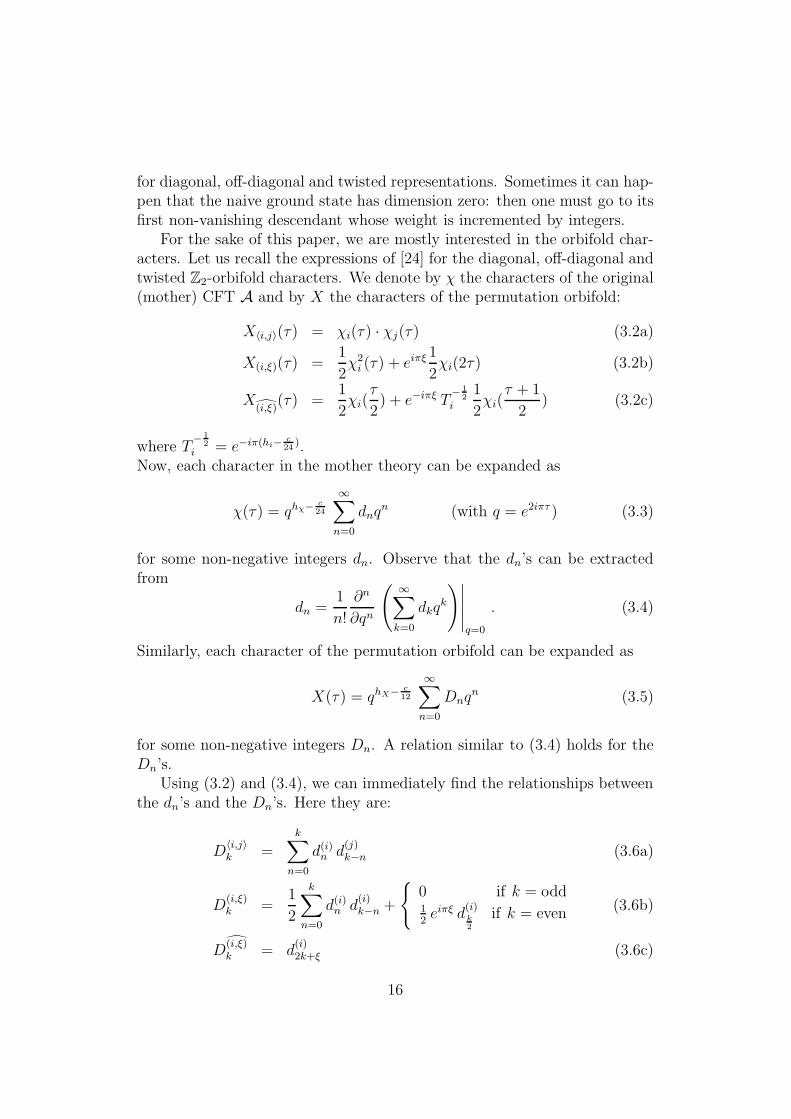
For the sake of this paper, we are mostly interested in the orbifold char-acters. Let us recall the expressions of [24] for the diagonal, off-diagonal andtwisted Z2-orbifold characters. We denote by χ the characters of the original(mother) CFT A and by X the characters of the permutation orbifold:

X〈i,j〉(τ) = χi(τ) · χj(τ) (3.2a)

X(i,ξ)(τ) =1

2χ2i (τ) + eiπξ

1

2χi(2τ) (3.2b)

X(i,ξ)

(τ) =1

2χi(

τ

2) + e−iπξ T

− 1

2

i

1

2χi(

τ + 1

2) (3.2c)

where T− 1

2

i = e−iπ(hi−c24

).Now, each character in the mother theory can be expanded as

χ(τ) = qhχ−c24

∞∑

n=0

dnqn (with q = e2iπτ ) (3.3)

for some non-negative integers dn. Observe that the dn’s can be extractedfrom

dn =1

n!

∂n

∂qn

(∞∑

k=0

dkqk

)∣∣∣∣∣q=0

. (3.4)

Similarly, each character of the permutation orbifold can be expanded as

X(τ) = qhX− c12

∞∑

n=0

Dnqn (3.5)

for some non-negative integers Dn. A relation similar to (3.4) holds for theDn’s.

Using (3.2) and (3.4), we can immediately find the relationships betweenthe dn’s and the Dn’s. Here they are:

D〈i,j〉k =

k∑

n=0

d(i)n d(j)k−n (3.6a)

D(i,ξ)k =

1

2

k∑

n=0

d(i)n d(i)k−n +

{

0 if k = odd12eiπξ d

(i)k2

if k = even(3.6b)

D(i,ξ)k = d

(i)2k+ξ (3.6c)

16

These expressions are particularly interesting because they tell us that, if wewant to have an expansion of the orbifold characters up to order k, then itis not enough to expand the original characters up to the same order k (itwould be enough for the untwisted fields), but rather we should go up to thehigher order 2k + 1, as it is implied by the third line of (3.6).

There are two possible reasons why a “naive” ground state dimensionmight vanish, so that the actual ground state weight is larger by some integervalue. If a ground state i has dimension one, the naive dimension of (i, 1)vanishes. Then the first non-trivial excited state will occur for the non-zerovalue of d

(i)n . Similarly, the conformal weight of an excited twist field (ξ = 1)

is larger than that of the unexcited one (ξ = 0) by half an integer, unlesssome odd excitations of the ground state vanish. In CFT, every state |φi〉,except the vacuum, always has an excited state L−1|φi〉. Furthermore, inN = 2 CFTs even the vacuum has an excited state J−1|0〉. Therefore, inN = 2 permutation orbifolds, the conformal weights of all ground states isequal to the typical values given above, except when a state |i〉 has groundstate dimension 1. Then the conformal weight is larger by one unit.

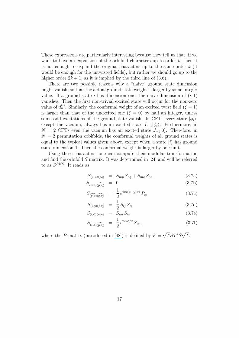
Using these characters, one can compute their modular transformationand find the orbifold S matrix. It was determined in [24] and will be referredto as SBHS . It reads as

S〈mn〉(pq) = Smp Snq + Smq Snp (3.7a)

S〈mn〉(p,χ)

= 0 (3.7b)

S(p,φ)(q,χ)

=1

2e2πi(φ+χ)/2 Pip (3.7c)

S(i,φ)(j,χ) =1

2Sij Sij (3.7d)

S(i,φ)〈mn〉 = Sim Sin (3.7e)

S(i,φ)(p,χ)

=1

2e2πiφ/2 Sip , (3.7f)

where the P matrix (introduced in [48]) is defined by P =√TST 2S

√T .

17

For future reference, it is convenient to recall the ansatz for the SJ ma-trices, as given in [27]:

S(J,ψ)〈mn〉(pq) = SJmp S

Jnq + (−1)ψSJmq S

Jnp (3.8a)

S(J,ψ)

〈mn〉(p,χ)=

{0 if J ·m = m

ASmp if J ·m = n(3.8b)

S(J,ψ)

(p,φ)(q,χ)= B

1

2eiπQJ (p) PJp,q e

iπ(φ+χ) (3.8c)

S(J,ψ)(i,φ)(j,χ) =

1

2SJij S

Jij (3.8d)

S(J,ψ)(i,φ)〈mn〉 = SJim S

Jin (3.8e)

S(J,ψ)

(i,φ)(p,χ)= C

1

2eiπφ Sip . (3.8f)

By modular invariance, the phases satisfy the following relations:

B = (−1)ψ e3iπhJ , A2 = C2 = (−1)ψ e2iπhJ , (3.9)

hJ being the weight of the simple current, which might depend on the centralcharge, rank and level of the original CFT. Note that B is fully fixed, whileA and C are fixed up to a sign. We choose the positive roots to get back theBHS S matrix as special case.

4 Permutations of N = 2 minimal models

In this section we consider the permutation orbifold of two N = 2 minimalmodels at level k. The CFT resulting from modding out the Z2 symmetry inthe tensor product (N = 2)k ⊗ (N = 2)k is known from [17, 18, 24]. Here wefocus mostly on the new interesting features arising when one extends thetheory with various simple currents.

As already mentioned, each N = 2 minimal model at level k admits asupersymmetric current TF (z) with ground state multiplicity equal to twoand spin h = 3

2. In the coset language, it corresponds to the NS field partner

of the identity, namely (l, m, s) = (0, 0, 2). This current transforms eachNS field into its NS partner (with different s) and each R field into its Rconjugate (corresponding to the other value of s). In order to see this, notethat the m and s indices are just u(1) labels, hence in the fusion of tworepresentations they simply add up: (s) × (s′) = (s + s′ mod4) and (m) ×(m′) = (m+m′ mod2(k + 2)).

The field TF (z) has simple fusion rules with any other field and it gen-erates two integer-spin simple currents in the permutation orbifold, corre-sponding to the symmetric and anti-symmetric representations (TF , 0) and

18

(TF , 1) of diagonal-type fields, both with spin h = 3. Both these currents canbe used to extend the permutation orbifold. They are both of order two and,interestingly (but not completely surprisingly), their product gives back theanti-symmetric representation of the identity:

(TF , 0) · (TF , 1) = (0, 1) , (4.1)

with all the other possible products obtained from this one by using cyclicityof the order two. In other words, the fields (0, 0), (TF , 0), (0, 1), (TF , 1) forma Z4 group under fusion.

We will study the extensions in the next two subsections, where we willalso see the new CFT structure coming from interchanging extensions andorbifolds. Before we do this, however, let us first mention some genericproperties of the orbifold. Consider the permutation orbifold of two N = 2minimal models at level k and extend it by either the symmetric or theanti-symmetric representation of TF (z). The resulting theory has the oldstandard simple currents coming from φ0,m,s (or equivalently φk,m+k+2,s+2,by the identification) in the mother theory (in number equal to the numberof simple currents of the (N = 2)k minimal model and corresponding to theorbits of their diagonal representations according to the fusion rules given inthe next two subsections) and an equal number of exceptional simple currentsthat were not simple currents before the extension (since coming from fixedoff-diagonal orbits of φ0,m,s, as we will see below).

The structure of the exceptional simple current is very generic: it is thesame for both (TF , 0) and (TF , 1), so we can consider both here. The wordexceptional means that they are simple currents just because their extended Smatrix satisfies the relation S0J = S00 [47]. First of all, note that the orbifoldsimple currents come from symmetric and anti-symmetric representations ofthe mother simple currents, hence there are as many as twice the number ofsimple currents of the mother minimal theory. Secondly, all the exceptionalcurrents correspond to the label l = 0 (or equivalently l = k) as it shouldbe, since related to the su(2)k algebra. This has the following consequence.Recall the orbifold (BHS) S matrix in the untwisted sector [24]:

SBHS(i,ψ)(j,χ) =1

2Sij Sij

SBHS(i,ψ)〈m,n〉 = Sim Sin

Using the minimal-model S matrix (2.30) one has:

S(0,0,0)(0,0,0) =1

2(k + 2)sin

(π

k + 2

)

= S(0,0,0)(0,m,s)

19

and henceSBHS((0,0,0),0),〈(0,m,s),(0,m,s+2)〉 = 2SBHS((0,0,0),0),((0,0,0),0) . (4.2)

This equality will soon be useful. In particular, the factor 2 will disappear inthe extension, promoting the off-diagonal fields 〈(0, m, s), (0, m, s+ 2)〉 intosimple currents. We will come back later to these exceptional currents.

Let us show now that these exceptional simple currents of the (TF , ψ)-extended orbifold correspond exactly to those particular off-diagonal fixed

points whose (TF , ψ)-orbits (ψ = 0, 1) are generated from the simple currentsof the mother N = 2 minimal model.Consider off-diagonal fields of the form 〈(0, m, s), (0, m, s + 2)〉. They arefixed points of (TF , ψ), since

4 TF · (0, m, s) = (0, m, s + 2). The number ofsuch orbits is equal to half the number of simple currents in the originalminimal model (i.e. those fields with l = 0). In the extension, they mustbe resolved. This means that each of them will give rise to two “split” fieldsin the extension. Hence their number gets doubled and one ends up witha number of split fields again equal to the number of simple currents ofthe original minimal model. Moreover, the extended S matrix, S, will beexpressed in terms of the SJ matrix corresponding to J ≡ (TF , ψ), accordingto

S(a,α)(b,β) = C · [SBHSab + (−1)α+β S(TF ,ψ)ab ] . (4.3)

Recall that the SJ matrix is non-zero only if the entries a and b are fixedpoints. The labels α and β keep track of the two split fields (α, β = 0 , 1).The factor C in front is a group theoretical quantity, that in case a and b areboth fixed, is equal to 1

2.

The generic formula for SJ as given in [27] was recalled in (3.7). Inparticular, the untwisted (i.e. diagonal and off-diagonal) entries of SJ vanish,since TF does not have fixed points:

S(TF ,ψ)〈m,n〉(p,q) = STFmp S

TFnq + (−1)ψSTFmq S

TFnp ≡ 0

S(TF ,ψ)(i,φ)(j,χ) =

1

2STFij STFij ≡ 0

S(TF ,ψ)(i,φ)〈m,n〉 = STFim STFin ≡ 0 .

This implies thatS(a,α)(b,β) = C · SBHSab (4.4)

for each split field corresponding to untwisted fixed points a, b. If either a orb are not fixed points, then S(TF ,ψ) is automatically zero and the S is givendirectly by SBHS, up to the overall group theoretical factor C in front, which

4This is proved in the next subsections.

20

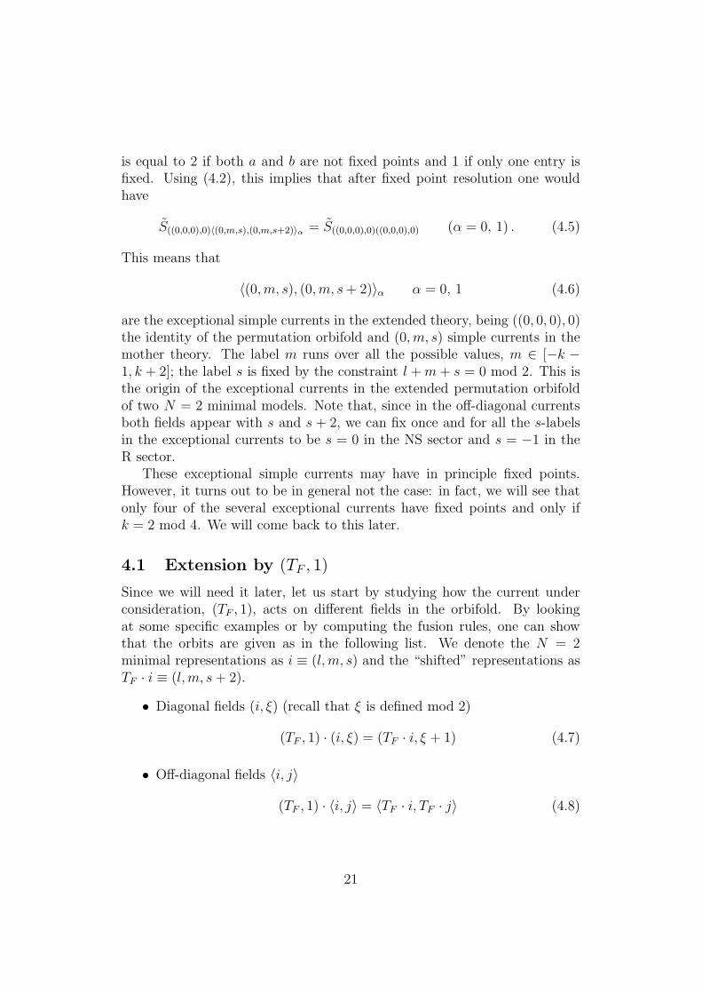
is equal to 2 if both a and b are not fixed points and 1 if only one entry isfixed. Using (4.2), this implies that after fixed point resolution one wouldhave

S((0,0,0),0)〈(0,m,s),(0,m,s+2)〉α = S((0,0,0),0)((0,0,0),0) (α = 0, 1) . (4.5)

This means that

〈(0, m, s), (0, m, s+ 2)〉α α = 0, 1 (4.6)

are the exceptional simple currents in the extended theory, being ((0, 0, 0), 0)the identity of the permutation orbifold and (0, m, s) simple currents in themother theory. The label m runs over all the possible values, m ∈ [−k −1, k + 2]; the label s is fixed by the constraint l +m+ s = 0 mod 2. This isthe origin of the exceptional currents in the extended permutation orbifoldof two N = 2 minimal models. Note that, since in the off-diagonal currentsboth fields appear with s and s + 2, we can fix once and for all the s-labelsin the exceptional currents to be s = 0 in the NS sector and s = −1 in theR sector.

These exceptional simple currents may have in principle fixed points.However, it turns out to be in general not the case: in fact, we will see thatonly four of the several exceptional currents have fixed points and only ifk = 2 mod 4. We will come back to this later.

4.1 Extension by (TF , 1)

Since we will need it later, let us start by studying how the current underconsideration, (TF , 1), acts on different fields in the orbifold. By lookingat some specific examples or by computing the fusion rules, one can showthat the orbits are given as in the following list. We denote the N = 2minimal representations as i ≡ (l, m, s) and the “shifted” representations asTF · i ≡ (l, m, s+ 2).

• Diagonal fields (i, ξ) (recall that ξ is defined mod 2)

(TF , 1) · (i, ξ) = (TF · i, ξ + 1) (4.7)

• Off-diagonal fields 〈i, j〉

(TF , 1) · 〈i, j〉 = 〈TF · i, TF · j〉 (4.8)

21

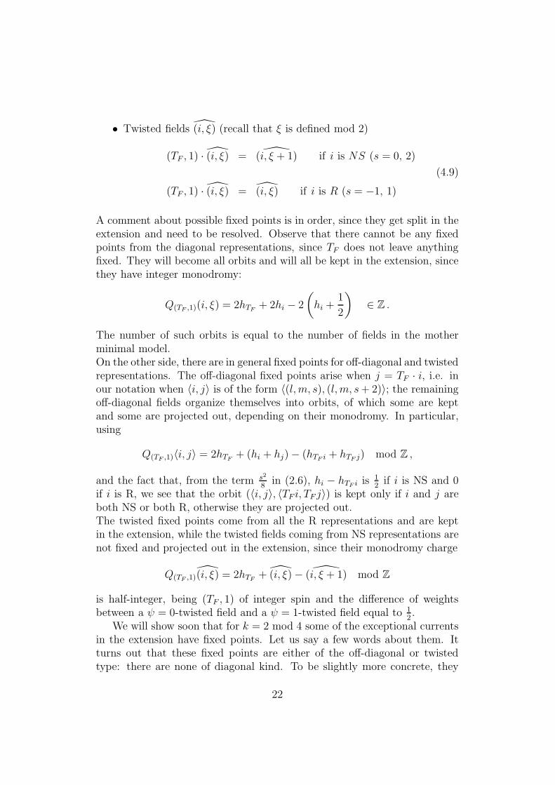
• Twisted fields (i, ξ) (recall that ξ is defined mod 2)

(TF , 1) · (i, ξ) = (i, ξ + 1) if i is NS (s = 0, 2)

(4.9)

(TF , 1) · (i, ξ) = (i, ξ) if i is R (s = −1, 1)

A comment about possible fixed points is in order, since they get split in theextension and need to be resolved. Observe that there cannot be any fixedpoints from the diagonal representations, since TF does not leave anythingfixed. They will become all orbits and will all be kept in the extension, sincethey have integer monodromy:

Q(TF ,1)(i, ξ) = 2hTF + 2hi − 2

(

hi +1

2

)

∈ Z .

The number of such orbits is equal to the number of fields in the motherminimal model.On the other side, there are in general fixed points for off-diagonal and twistedrepresentations. The off-diagonal fixed points arise when j = TF · i, i.e. inour notation when 〈i, j〉 is of the form 〈(l, m, s), (l, m, s+ 2)〉; the remainingoff-diagonal fields organize themselves into orbits, of which some are keptand some are projected out, depending on their monodromy. In particular,using

Q(TF ,1)〈i, j〉 = 2hTF + (hi + hj)− (hTF i + hTF j) mod Z ,

and the fact that, from the term s2

8in (2.6), hi − hTF i is

12if i is NS and 0

if i is R, we see that the orbit (〈i, j〉, 〈TF i, TF j〉) is kept only if i and j areboth NS or both R, otherwise they are projected out.The twisted fixed points come from all the R representations and are keptin the extension, while the twisted fields coming from NS representations arenot fixed and projected out in the extension, since their monodromy charge

Q(TF ,1)(i, ξ) = 2hTF + (i, ξ)− (i, ξ + 1) mod Z

is half-integer, being (TF , 1) of integer spin and the difference of weightsbetween a ψ = 0-twisted field and a ψ = 1-twisted field equal to 1

2.

We will show soon that for k = 2 mod 4 some of the exceptional currentsin the extension have fixed points. Let us say a few words about them. Itturns out that these fixed points are either of the off-diagonal or twistedtype: there are none of diagonal kind. To be slightly more concrete, they

22

are specific (TF , 1)-orbits of off-diagonal fields plus all the twisted (TF , 1)-fixed points (necessarily corresponding to the Ramond fields of the originalminimal model). We will not say more now, but will come back later. At themoment we are not able to resolve them: in other words, we do not knowwhat their SJ matrices are, J denoting the particular exceptional currents.

One important exceptional currents of the permutation orbifold is theworldsheet supersymmetry current, which is the only current of order twoand spin h = 3

2: it is the off-diagonal field coming from the tensor product

of the identity with TF (z). It does not have fixed points, because TF doesnot. Let us denote it by Jw.s.orb ≡ 〈0, TF 〉. By the argument given above, Jw.s.orb

is guaranteed to be fixed by (TF , 1). This means that in the extension it getssplit into two fields, that we denote by 〈0, TF 〉α, with α = 0 or 1. In theappendix we check that indeed 〈0, TF 〉α has order two:

〈0, TF 〉α · 〈0, TF 〉α = (0, 0) , (4.10)

where (0, 0) is the identity orbit.Now consider the tensor product of two minimal models. We can either

extend by TF (z)⊗TF (z) to make the product supersymmetric or we can modout the Z2 symmetry and end up with the permutation orbifold. Let us startwith the latter option. It is known [27] that one can go back to the tensorproduct by extending the orbifold by the anti-symmetric representation of theidentity, (0, 1). What we do instead is extending the orbifold by (TF , 1). Theresulting theory is the N = 2 supersymmetric permutation orbifold whichhas the worldsheet spin-3

2current in its spectrum.

Alternatively, we can change the order and perform the extension beforeorbifolding. Note that each N = 2 factor is supersymmetric, but the productis not. In order to make it supersymmetric, we have to extend it by thetensor-product current TF (z) ⊗ TF (z). As a result, in the tensor productonly those fields survive whose two factors are either both in the NS orboth in the R sector. In this way, the fields in the product have factorsthat are aligned to be in the same sector. Now we still have to take theZ2 orbifold. Starting from the supersymmetric product, by definition, welook for Z2-invariant states/combinations and add the proper twisted sector.We will refer to this mechanism which transform the supersymmetric tensorproduct into the supersymmetric orbifold as super-BHS, in analogy with thestandard BHS from the tensor product to the orbifold. The following scheme

23

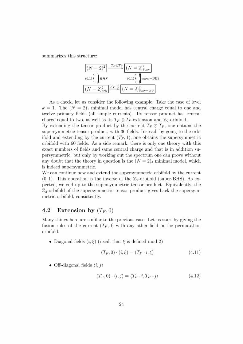
summarizes this structure:

(N = 2)2

BHS��

TF⊗TF // (N = 2)2Susy

super−BHS

��

(N = 2)2orb

(0,1)

KK

(TF ,1)// (N = 2)2Susy−orb

(0,1)

KK

As a check, let us consider the following example. Take the case of levelk = 1. The (N = 2)1 minimal model has central charge equal to one andtwelve primary fields (all simple currents). Its tensor product has centralcharge equal to two, as well as its TF ⊗ TF -extension and Z2-orbifold.By extending the tensor product by the current TF ⊗ TF , one obtains thesupersymmetric tensor product, with 36 fields. Instead, by going to the orb-ifold and extending by the current (TF , 1), one obtains the supersymmetricorbifold with 60 fields. As a side remark, there is only one theory with thisexact numbers of fields and same central charge and that is in addition su-persymmetric, but only by working out the spectrum one can prove withoutany doubt that the theory in question is the (N = 2)4 minimal model, whichis indeed supersymmetric.We can continue now and extend the supersymmetric orbifold by the current(0, 1). This operation is the inverse of the Z2-orbifold (super-BHS). As ex-pected, we end up to the supersymmetric tensor product. Equivalently, theZ2-orbifold of the supersymmetric tensor product gives back the supersym-metric orbifold, consistently.

4.2 Extension by (TF , 0)

Many things here are similar to the previous case. Let us start by giving thefusion rules of the current (TF , 0) with any other field in the permutationorbifold.

• Diagonal fields (i, ξ) (recall that ξ is defined mod 2)

(TF , 0) · (i, ξ) = (TF · i, ξ) (4.11)

• Off-diagonal fields 〈i, j〉

(TF , 0) · 〈i, j〉 = 〈TF · i, TF · j〉 (4.12)

24

• Twisted fields (i, ξ) (recall that ξ is defined mod 2)

(TF , 0) · (i, ξ) = (i, ξ) if i is NS (s = 0, 2)

(4.13)

(TF , 0) · (i, ξ) = (i, ξ + 1) if i is R (s = −1, 1)

Again, the current (TF , 0) does not have diagonal fixed points, but does haveoff-diagonal and twisted fixed points. The off-diagonal ones are like before,while the twisted ones come this time from NS fields. Twisted fields comingfrom R representations are projected out in the extension. Each fixed pointis split in two in the extended permutation orbifold and must be resolved.Moreover, there will also be orbits coming from the diagonal and off-diagonalfields.

Also for (TF , 0)-extensions a few exceptional currents might have fixedpoints. They are either off-diagonal (TF , 0)-orbits or all the twisted (TF , 0)-fixed points (necessarily of Neveu-Schwarz origin).

As before, consider now the tensor product of two minimal models andits permutation orbifold. Extend the orbifold with the current (TF , 0), i.e.the symmetric representation TF (z). One obtains a new, for the momentmysterious, CFT that we denote by X . X is not supersymmetric, since itdoes not contain the worldsheet supercurrent of spin h = 3

2. To be more

precise, X does contain a spin 32-current, which is again the off-diagonal

field 〈0, TF 〉. However, it is not the worldsheet supersymmetry current. Thereason is that in this case 〈0, TF 〉 (or rather the two split fields 〈0, TF 〉α,with α = 0 or 1) has order 4, instead of order 2: acting twice with Jw.s.orb (z)we should get back to the same field, but we do not. As we prove in theappendix:

〈0, TF 〉α · 〈0, TF 〉α = (0, 1) , (4.14)

with (0, 1) · (0, 1) = (0, 0). Hence there is no such a current as Jw.s.orb (z) inX . Continuing extending this time by the current (0, 1) we get back to thefamiliar theory (N = 2)2Susy. The summarizing graph is below:

(N = 2)2

BHS��

TF⊗TF // (N = 2)2Susy

(N = 2)2orb

(0,1)

KK

(TF ,0) // Non− Susy X

(0,1)

OO

25

4.3 Common properties

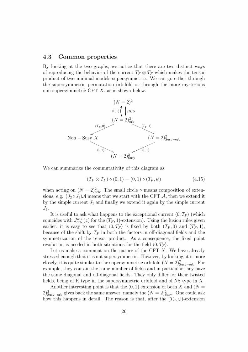
By looking at the two graphs, we notice that there are two distinct waysof reproducing the behavior of the current TF ⊗ TF which makes the tensorproduct of two minimal models supersymmetric. We can go either throughthe supersymmetric permutation orbifold or through the more mysteriousnon-supersymmetric CFT X , as is shown below.

(N = 2)2

BHS

(N = 2)2orb

(0,1)

JJ

(TF ,0)

vvmmmmmmmmmmmmm(TF ,1)

((QQQQQQQQQQQQ

Non− Susy X

(0,1) ((PPPPPPPPPPPPP

(N = 2)2Susy−orb

(0,1)vvmmmmmmmmmmmm

(N = 2)2Susy

We can summarize the commutativity of this diagram as:

(TF ⊗ TF ) ◦ (0, 1) = (0, 1) ◦ (TF , ψ) (4.15)

when acting on (N = 2)2orb. The small circle ◦ means composition of exten-sions, e.g. (J2 ◦J1)A means that we start with the CFT A, then we extend itby the simple current J1 and finally we extend it again by the simple currentJ2.

It is useful to ask what happens to the exceptional current 〈0, TF 〉 (whichcoincides with Jw.s.orb (z) for the (TF , 1)-extension). Using the fusion rules givenearlier, it is easy to see that 〈0, TF 〉 is fixed by both (TF , 0) and (TF , 1),because of the shift by TF in both the factors in off-diagonal fields and thesymmetrization of the tensor product. As a consequence, the fixed pointresolution is needed in both situations for the field 〈0, TF 〉.

Let us make a comment on the nature of the CFT X . We have alreadystressed enough that it is not supersymmetric. However, by looking at it moreclosely, it is quite similar to the supersymmetric orbifold (N = 2)2Susy−orb. Forexample, they contain the same number of fields and in particular they havethe same diagonal and off-diagonal fields. They only differ for their twistedfields, being of R type in the supersymmetric orbifold and of NS type in X .

Another interesting point is that the (0, 1) extension of both X and (N =2)2Susy−orb gives back the same answer, namely the (N = 2)2Susy. One could askhow this happens in detail. The reason is that, after the (TF , ψ)-extension

26

(either ψ = 0 or 1) of the orbifold, one is left with orbits and/or fixed pointscorresponding to orbifold fields of diagonal, off-diagonal and twisted type.In particular, as we already mentioned before, from the twisted fields onlythe fixed points survive, with the difference that for ψ = 1 they come fromthe Ramond sector and for ψ = 0 from the NS sector. However, they arecompletely projected out by the (0, 1)-extension, which leaves only untwisted(i.e. off-diagonal and diagonal -both symmetric and anti-symmetric-) fieldsin the supersymmetric tensor product5.

5 Exceptional simple currents and their fixed

points

Let us be a bit more precise on the exceptional simple currents which admitfixed points. There are four of them and they are always related to thefollowing mother-theory simple currents

J+ ≡ (l, m, s) ≡ (0,k + 2

2, s) ≡ (k,−k + 2

2, s+ 2) (5.1)

and

J− ≡ (0,−k + 2

2, s) ≡ (k,

k + 2

2, s+ 2) (5.2)

(with s = 0 in the NS sector, s = −1 in the R sector). We will soon provethat s must be in the NS sector. i.e. s = 0, otherwise there are no fixedpoints. Using the facts that m is defined mod 2(k + 2) and that s is definedmod 4, together with the identification (l, m, s) = (k − l, m + k + 2, s + 2),it is easy to show that J+ and J− are of order four, i.e. J4

+ = J4− = 1.

Moreover, we will soon show that off-diagonal fixed points of the exceptionalcurrents originate from fields in the mother N = 2 theory with l-label equalto l = k

2. One can easily check that, on these fields, the square of J±, J

2±,

acts as follows. For J± in the R sector, J2± fixes any other field (either R or

NS) of the original minimal model:

(J± ∈ R) J2± : (l =

k

2, m, s) −→ (l =

k

2, m, s) =⇒ J2

± ≃ 1 ≡ (0, 0, 0) ,

(5.3)

5The reason is that the current (0, 1) always couples a twisted field (p, 0) to its partner

(p, 1), as it is shown in the appendix. Since these fields have weights which differ by 1

2, then

their monodromy will be half-integer and they will be projected out in the (0, 1)-extension.

27

acting on them effectively as the identity; for J± in the NS sector, J2± takes

an R (NS) field into its conjugate R (NS) field:

(J± ∈ NS) J2± : (l =

k

2, m, s) −→ (l =

k

2, m, s+2) =⇒ J2

± ≃ TF ≡ (0, 0, 2) ,

(5.4)acting effectively as the supersymmetry current.

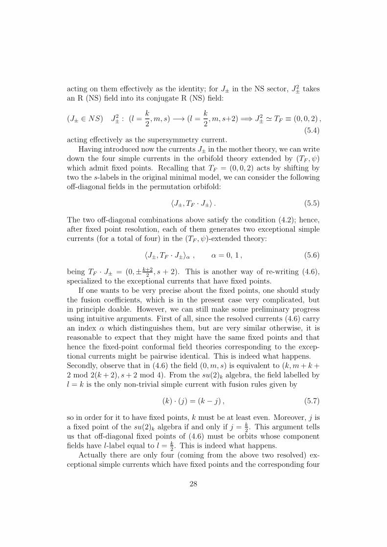
Having introduced now the currents J± in the mother theory, we can writedown the four simple currents in the orbifold theory extended by (TF , ψ)which admit fixed points. Recalling that TF = (0, 0, 2) acts by shifting bytwo the s-labels in the original minimal model, we can consider the followingoff-diagonal fields in the permutation orbifold:

〈J±, TF · J±〉 . (5.5)

The two off-diagonal combinations above satisfy the condition (4.2); hence,after fixed point resolution, each of them generates two exceptional simplecurrents (for a total of four) in the (TF , ψ)-extended theory:

〈J±, TF · J±〉α , α = 0, 1 , (5.6)

being TF · J± = (0,±k+22, s + 2). This is another way of re-writing (4.6),

specialized to the exceptional currents that have fixed points.If one wants to be very precise about the fixed points, one should study

the fusion coefficients, which is in the present case very complicated, butin principle doable. However, we can still make some preliminary progressusing intuitive arguments. First of all, since the resolved currents (4.6) carryan index α which distinguishes them, but are very similar otherwise, it isreasonable to expect that they might have the same fixed points and thathence the fixed-point conformal field theories corresponding to the excep-tional currents might be pairwise identical. This is indeed what happens.Secondly, observe that in (4.6) the field (0, m, s) is equivalent to (k,m+ k+2 mod 2(k+ 2), s+ 2 mod 4). From the su(2)k algebra, the field labelled byl = k is the only non-trivial simple current with fusion rules given by

(k) · (j) = (k − j) , (5.7)

so in order for it to have fixed points, k must be at least even. Moreover, j isa fixed point of the su(2)k algebra if and only if j = k

2. This argument tells

us that off-diagonal fixed points of (4.6) must be orbits whose componentfields have l-label equal to l = k

2. This is indeed what happens.

Actually there are only four (coming from the above two resolved) ex-ceptional simple currents which have fixed points and the corresponding four

28

fixed-point conformal field theories are pairwise identical. Indeed, the ex-ceptional simple currents have m-label equal to m = ±k+2

2, even s-label and

hence the generic constraints l+m+ s = 0 mod 2 implies that k = 2 mod 4.Let us describe more in detail the exceptional simple currents with fixed

points. Consider again (5.6) and study the fusion rules of (5.5). We are mostinterested in off-diagonal fixed points, because they have an interesting struc-ture; as far as the other kind (namely twisted) of fixed points is concerned,they are as already reported in the previous section (namely of NS type for(TF , 0) and of R type for (TF , 1)). Compute the fusion rule of the current(J±, TFJ±) with any field of the form:

〈f, J±f ′〉 , (5.8)

where f ′ has either the same s-label as f or different; in other words, eitherf ′ = f or f ′ = TFf . Here, f and f ′ label primaries of the original N = 2minimal model which might be fixed points of (5.6), having their l-valuesequal to l = k

2. Explicitly, f = (k

2, m, s) and f ′ = (k

2, m, s′),with s′ = s or

s′ = s+ 2.We would like to show that the fields 〈f, J±f ′〉 constitute the subset of

off-diagonal fixed points for the exceptional currents. For most of them,this subset will be empty, but not for (5.6). As a remark, note that not allthe fields in (5.8) are independent, since they are identified pairwise by theextension. We will come back to this at the end of this subsection.

Now let us compute the fusion rules. Naively:

〈J±, TFJ±〉 · 〈f, J±f ′〉 ∝ (J± ⊗ TFJ± + TFJ± ⊗ J±) · (f ⊗ J±f′ + J±f

′ ⊗ f)

= (J±f ⊗ TFf′ + J2

±f′ ⊗ TFJ±f +

+TFJ±f ⊗ J2±f

′ + TFJ2±f

′ ⊗ J±f) .

For currents in the R sector, J2± = 1, while J2

± = TF in the NS sector; hencethe above expression simplifies in both cases:

〈J±, TFJ±〉·〈f, J±f ′〉 ∝ · · · =

(J±f ⊗ TFf′ + f ′ ⊗ TFJ±f+ R sector

+TFJ±f ⊗ f ′ + TFf′ ⊗ J±f) .

(J±f ⊗ f ′ + TFf′ ⊗ TFJ±f+ NS sector

+TFJ±f ⊗ TFf′ + f ′ ⊗ J±f)

In terms of representation, we can decompose the r.h.s. in two pieces corre-sponding to the following symmetric representations:

(R) 〈J±, TFJ±〉 · 〈f, J±f ′〉 = 〈J±f, TFf ′〉+ 〈f ′, TFJ±f〉(NS) 〈J±, TFJ±〉 · 〈f, J±f ′〉 = 〈f ′, J±f〉+ 〈TFf ′, TFJ±f〉 (5.9)

29

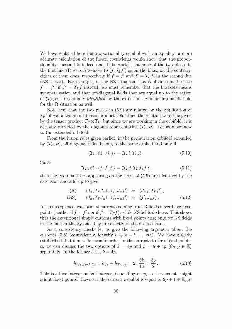
We have replaced here the proportionality symbol with an equality: a moreaccurate calculation of the fusion coefficients would show that the propor-tionality constant is indeed one. It is crucial that none of the two pieces inthe first line (R sector) reduces to (f, J±f

′) as on the l.h.s.; on the contrary,either of them does, respectively if f = f ′ and f ′ = TFf , in the second line(NS sector). For example, in the NS situation, this is obvious in the casef = f ′; if f ′ = TFf instead, we must remember that the brackets meanssymmetrization and that off-diagonal fields that are equal up to the actionof (TF , ψ) are actually identified by the extension. Similar arguments holdfor the R situation as well.

Note here that the two pieces in (5.9) are related by the application ofTF : if we talked about tensor product fields then the relation would be givenby the tensor product TF ⊗TF , but since we are working in the orbifold, it isactually provided by the diagonal representation (TF , ψ). Let us move nowto the extended orbifold.

From the fusion rules given earlier, in the permutation orbifold extendedby (TF , ψ), off-diagonal fields belong to the same orbit if and only if

(TF , ψ) · 〈i, j〉 = 〈TF i, TF j〉 . (5.10)

Since(TF , ψ) · 〈f, J±f ′〉 = 〈TFf, TFJ±f ′〉 , (5.11)

then the two quantities appearing on the r.h.s. of (5.9) are identified by theextension and add up to give

(R) 〈J±, TFJ±〉 · 〈f, J±f ′〉 = 〈J±f, TFf ′〉 ,(NS) 〈J±, TFJ±〉 · 〈f, J±f ′〉 = 〈f ′, J±f〉 . (5.12)

As a consequence, exceptional currents coming from R fields never have fixedpoints (neither if f = f ′ nor if f ′ = TFf), while NS fields do have. This showsthat the exceptional simple currents with fixed points arise only for NS fieldsin the mother theory and they are exactly of the desired form.

As a consistency check, let us give the following argument about thecurrents (5.6) (equivalently, identify l → k − l , . . . etc). We have alreadyestablished that k must be even in order for the currents to have fixed points,so we can discuss the two options of k = 4p and k = 2 + 4p (for p ∈ Z)separately. In the former case, k = 4p,

h〈J±,TF ·J±〉α = hJ± + hTF ·J± = 2 · 3k16

=3p

2. (5.13)

This is either integer or half-integer, depending on p, so the currents mightadmit fixed points. However, the current m-label is equal to 2p + 1 ∈ Zodd;

30

since the l-label is even, then the N = 2 constraint forces the s-label to be±1. As a consequence, the currents (5.6) are of Ramond-type and hencecannot have fixed points. In the latter case, k = 2 + 4p,

h〈J±,TF ·J±〉α = hJ± + hTF ·J± =

(3k

16− 1

8

)

+

(3k

16+

3

8

)

= 1 +3p

2. (5.14)

This is either integer or half-integer, depending on p, then the current canhave fixed points. Moreover, since the m-label is equal to 2p+2 ∈ Zeven, thecurrents (5.6) are now of NS-type, hence they will have fixed points.

Needless to say, we do expect all a priori possible fields of the form (5.8)to survive the (TF , ψ)-extension, the reason being that their (TF , ψ)-orbitsmust have zero monodromy charge with respect to the current (TF , ψ). As anexercise, let us compute this charge and prove that it vanishes (mod integer).For this purpose, we need to know the weight of (5.8). Since

hJ±f = hf −1

16(k + 2± 4m) (5.15)

m being the m-label of the field f , then

h〈f,J±f ′〉 = hf + hJ±f ′ = 2hf −1

8(k + 2± 4m) +

1

2δf ′,TF f . (5.16)

Similarly, we need to compute hTF f,TF J±f ′. Since

hTF J±f = hTF f −1

16(k + 2± 4m) (5.17)

then again

h〈TF f,TF J±f ′〉 = hTF f + hTF J±f ′ = 2hTF f −1

8(k + 2± 4m) +

1

2δf ′,TF f . (5.18)

Hence:

Q(TF ,ψ)

(〈f, J±f ′〉

)= h(TF ,ψ) + h〈f,J±f ′〉 − h〈TF f,TF J±f ′〉 = 0 , (5.19)

i.e. these fields are kept in the extension and organize themselves into orbits.Still, some fields seem not to appear among the off-diagonal field that wewould expect. The solutions to this problem is provided by the extension:fields are pairwise identified. In fact, as a consequence of (5.9), two fieldsrelated by the action of (5.5) are mapped into each other by (TF , ψ) andhence are identified by the currents (5.6) in the extension.

31

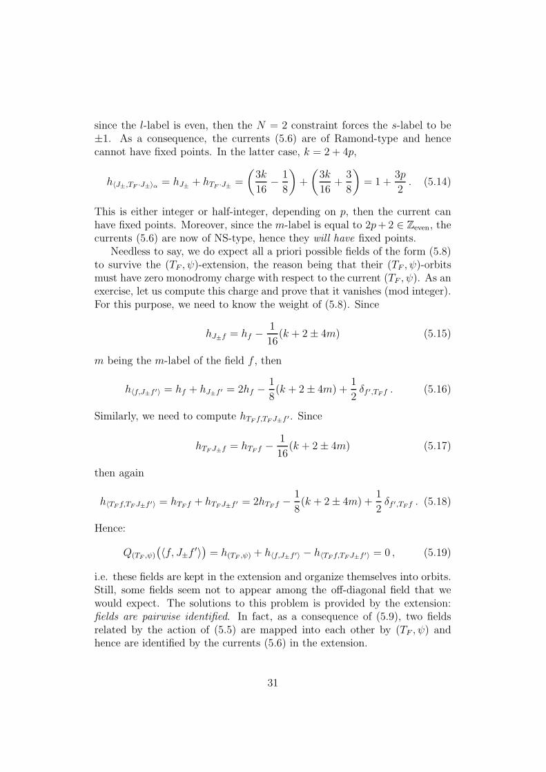
What happens in determining the fixed points of the exceptional currentsis the following. Start with a field f which has l-label equal to k

2and apply

J± on f , recalling that J4± = 1 and J2

± = TF for NS-type currents,

fJ±

��J±TFf

J±55

J±f

J±wwTFf

J±

]]

as shown in the graph. The four fields organize themselves pairwise into twoJ±-orbits which are related by the action of TF , or better of (TF , ψ). In fact,from the fusion rules of (TF , ψ) with off-diagonal fields it follows that

(TF , ψ) · 〈f, J±f〉 = 〈TFf, J±TFf〉 . (5.20)

Each J±-orbit has the same form as (5.8). In the (TF , ψ)-extension they areidentified and becomes fixed points of the exceptional simple currents (5.6).Similarly, we can organize the fields differently. For instance, by startingfrom the J±-orbit 〈f, J±TFf〉, we have

(TF , ψ) · 〈f, J±TFf〉 = 〈TFf, J±f〉 , (5.21)

where we used T 2F = 1. The same argument holds if we start from any J±-

orbit of two consecutive fields in the graph above: the (TF , ψ)-extension willalways identify it with the remaining orbit.

In the next subsection we give and explicit example corresponding to the“easy” case of minimal models at level two.

5.1 k = 2 Example

In order to better visualize the structure of exceptional simple currents andtheir fixed points, let us consider the k = 2 case, where we permute twoN = 2 minimal models at level two. This case is easy enough to be workedout explicitly, but complicated enough to show all the desired properties.This minimal model has 24 fields (12 in the R sector and 12 in the NS sector),of which 16 simple currents. Using [17, 24, 27], its permutation orbifold hasgot 372 fields, of which 32 simple currents coming from diagonal (symmetricand anti-symmetric) combinations of the original simple currents. The oneswith (half-)integer spin have generically got fixed points which we know howto resolve [27].

32

In the (TF , ψ)-extended orbifold theory, the exceptional currents withfixed points are

〈J±, TF · J±〉α , α = 0, 1 , (5.22)

withJ+ = (0, 2, 0) and J− = (0,−2, 0) . (5.23)

Their off-diagonal fixed points are of the form

〈f, J±f ′〉 , (5.24)

with f and J±f′ given by

f = (1, 1, 0) and f ′ = (1,−1, 0)

f = (1, 2, 1) and f ′ = (1, 0, 1)

f = (1,−1, 0) and f ′ = (1, 1, 2)

f = (1, 2, 1) and f ′ = (1, 0,−1)

To these, we still have to add the twisted fixed points, but we know alreadyexactly what they are. One can observe that some fields appear twice, e.g.(1, 2, 1), and other fields never appear, e.g. (1, 2,−1). This can be easilyexplained. The reason why some of them appear more than once is becausef and f ′ can have either equal or different s-values (J± only acts on them-values).Similarly, some fields are identified by the (TF , ψ)-extension and hence theyseem never to appear. For example, the off-diagonal field 〈(1, 2,−1), (1, 0, 1)〉seems not to be there, but it is actually identified with 〈(1, 2, 1), (1, 0,−1)〉,which appears in the last line of the list above; similarly 〈(1, 2,−1), (1, 0,−1)〉seems again not to be there as well, but it is identified with 〈(1, 2, 1), (1, 0, 1)〉which is there in the second line of the same list.

More in general, this is a consequence of (5.9). In the present situationwe see this explicitly. Let us look at the current

〈(0, 2, 0), (0, 2, 2)〉 (5.25)

in the permutation orbifold and compute its fusion rules with the off-diagonalfield 〈(1, 2,−1), (1, 0, 1)〉:

〈(0, 2, 0), (0, 2, 2)〉·〈(1, 2,−1), (1, 0, 1)〉= 〈(1, 2,−1), (1, 0, 1)〉+〈(1, 2, 1), (1, 0,−1)〉 .(5.26)

We see the appearance of the second term on the r.h.s., which is also anoff-diagonal field, so we are led to ask about its fusion as well:

〈(0, 2, 0), (0, 2, 2)〉·〈(1, 2, 1), (1, 0,−1)〉= 〈(1, 2,−1), (1, 0, 1)〉+〈(1, 2, 1), (1, 0,−1)〉 ,(5.27)

33

which is exactly the same as the first one. However, observe that the current(TF , ψ) relates the two terms on both r.h.s.’s:

(TF , ψ) · 〈(1, 2,−1), (1, 0, 1)〉 = 〈(1, 2, 1), (1, 0,−1)〉(TF , ψ) · 〈(1, 2, 1), (1, 0,−1)〉 = 〈(1, 2,−1), (1, 0, 1)〉 . (5.28)

Then, they form one orbit in the (TF , ψ)-extension and, since they haveinteger monodromy charge, this off-diagonal orbit survives the projection.Due to (5.26) and (5.27), this orbit becomes an off-diagonal fixed point ofthe exceptional current.

As a comment, we remark that it is not known at the moment how toresolve these fixed points. The reason is that they are fixed points of anoff-diagonal current for which there is no solution yet, unlike for the fixedpoints of diagonal currents for which the solution exists and was provided in[27].

6 Orbit structure for N = 2 and N = 1

Here we want to summarize the simple current orbits for theories consideredhere, and give the analogous results for N = 1 minimal models for compari-son. Most of the construction, and in particular the definition of the six kindsof CFT listed in the introduction works completely analogously for N = 2and N = 1. The worldsheet supercurrent, originating from the diagonal field〈0, TF 〉, comes in both cases from a fixed point. However, a novel featureoccurring for N = 1 but not for N = 2 is that this supercurrent itself hasfixed points whose resolution requires additional data.

Another important difference between the N = 2 and N = 1 permu-tation orbifolds is that in the latter case the supersymmetric and the non-supersymmetric orbifold (the extensions of the BHS orbifold by (TF , 1) or(TF , 0) respectively) have a different number of primaries, whereas for N = 2this is the same.

The simple current groups of all these theories are as described below. Afew currents always play a special role, namely

• The “un-orbifold” current. This is the current that undoes the permu-tation orbifold. In the BHS orbifold this is the anti-symmetric diagonalfield (0, 1), which has spin-1. If the theories are extended by (TF , 1)or (TF , 0) this field becomes part of a larger module, but is still theground state of that module.

• The worldsheet supercurrent(s). This has always weight 32, and can

have fixed points only for N = 1 (and then it usually does). The su-

34

persymmetric permutation orbifolds always have two of them, whichoriginate from the split fixed points of the off-diagonal field 〈0, TF 〉.Note that this multiplicity, two, has nothing to do with the number ofsupersymmetries. The latter is given by the dimension of the groundstate of the supercurrent module. The fusion product of the two super-currents is always the un-orbifold current. These spin-3

2currents also

occur in the non-supersymmetric theory X , except in that case theygenerate a Z4 group, whereas in the supersymmetric case the discretegroup they generate is Z2 × Z2.

• The Ramond ground state simple currents. These exist only for theN = 2 and not for the N = 1 superconformal models.

In the following we call a fixed point “resolvable” if we have explicitformulas for the fixed point resolution matrices, and unresolvable otherwise.Therefore, “unresolvable” does not mean that the fixed points cannot beresolved in principle, but simply that it is not yet known how to do it. Notethat the choices of generators of discrete groups described below are notunique, but we made convenient choices. As much as possible, we try tochoose the special currents listed above as generators of the discrete groupfactors.

• N = 2, k = 1 mod 2.

– The minimal models have a simple current group Z4k+8. As itsgenerator one can take the Ramond ground state simple current.The power 2k+4 of this generator is the worldsheet supercurrent.None of the simple current has fixed points.

– The supersymmetric permutation orbifold has a group structureZ4k+8 × Z2. The first factor is generated by the Ramond groundstate simple current. The power 2k + 4 of this generator is theun-orbifold current. This is the only current that has fixed points,which are resolvable. The factor Z2 is generated by the worldsheetsupercurrent.

– The non-supersymmetric permutation orbifold X also has a groupstructure Z4k+8 × Z2. The spin-3

2fields originating from the di-

agonal field 〈0, TF 〉 have order 4, and generate a Zk+2 subgroupof Z4k+8. The order-two element of Z4k+8 is, just as above, theun-orbifold current. Also in this case it has resolvable fixed points.

• N = 2, k = 0 mod 4.

35

– The minimal models have a simple current group Z2k+4 × Z2. Asthe generator of the first factor one can take the Ramond groundstate simple current, and the worldsheet supercurrent can be usedas the generator of the second. The middle element of the Z2k+4

factor is an integer spin current with resolvable fixed points.

– The supersymmetric permutation orbifold has a group structureZ2k+4 × Z2 × Z2. The first factor is generated by the Ramondground state simple current. The second factor by the un-orbifoldcurrent. The last factor is generated by the worldsheet supercur-rent. The middle element of the first factor and the generator ofthe second factor, as well as their product have resolvable fixedpoints.

– The non-supersymmetric permutation orbifoldX has a group struc-ture Z2k+4 × Z4. The spin-3

2fields originating from the diagonal

field 〈0, TF 〉 have order 4 can be chosen as generators of the Z4

factor. There are three non-trivial currents with resolvable fixedpoints, which have the same origin (in terms of minimal modelfields) as the ones in the supersymmetric orbifold.

• N = 2, k = 2 mod 4.

– The minimal models have a simple current group Z2k+4×Z2. Thestructure is exactly as for k = 0 mod 4.

– The supersymmetric permutation orbifold has a group structureZ2k+4 × Z2 × Z2. One can choose the same generators as abovefor k = 0 mod 4. The fixed point structure is also identical,except that there are four additional currents with unresolvablefixed points. These four currents are the two order 4 currents ofZ2k+4 multiplied with each of the two world-sheet supercurrents.

– The non-supersymmetric permutation orbifoldX has a group struc-ture Z2k+4 × Z4. As in the supersymmetric case, there are threenon-trivial currents with resolvable fixed points, and four withunresolvable fixed points. These currents have the same origin asthose of the supersymmetric orbifold.

• N = 1, k = 1 mod 2.

– The minimal models have a simple current group Z2, generatedby the worldsheet supercurrent. This current has resolvable fixedpoints.

36

– The supersymmetric permutation orbifold has a group structureZ2 × Z2. The two factors can be generated by the un-orbifoldcurrent and by the worldsheet current. The fourth element alsohas spin-3

2, and is an alternative worldsheet supercurrent. The

un-orbifold current has resolvable fixed points, the supercurrentshave unresolvable fixed points.

– The non-supersymmetric permutation orbifoldX has a group struc-ture Z8. The order-2 element in this subgroup is the un-orbifoldcurrent, which has resolvable fixed points. None of the other cur-rents have fixed points.

• N = 1, k = 0 mod 2.

– The minimal models have a simple current group Z2×Z2. All cur-rents have resolvable fixed points. One of them is the worldsheetsupercurrent.

– The supersymmetric permutation orbifold has a group structureZ2 × Z2 × Z2. Two of the three factors are generated by theun-orbifold current and one of the worldsheet supercurrents. Allcurrents have fixed points, and for four of them, including thesupersymmetry generators, they are unresolvable.

– The non-supersymmetric permutation orbifoldX has a group struc-ture Z4 ×Z2. All currents have fixed points, and for four of themthey are unresolvable.

7 Conclusion

In this paper we study permutation and extensions of N = 2 minimal modelsat arbitrary level k. These models are very interesting for several reason: notonly because they are non-trivial solvable conformal field theories, but alsobecause they are the building blocks of Gepner models which have somerelevance in string theory phenomenology.

Our main points are two. First of all, a new structure arises relatingconformal field theories built out of minimal models. Starting from the ten-sor product we perform Z2-orbifold and extension in both possible orders,generating in this way new CFT. Some of them are easily recognizable, suchas the N = 2 supersymmetric orbifold obtained by extending the standardpermutation orbifold by the current (TF , 1). Some others are however notknown, like the CFT that we have denoted by X , obtained by extending theorbifold by (TF , 0).

37

Secondly, unexpected off-diagonal simple currents appear due to the in-terplay of the orbifold and the extension procedure. Sometimes they havefixed points that need to be resolved. However, because they are related tooff-diagonal currents, we do not know how to resolve them at the moment.

The most natural and immediate application of our method is to considerpermutation orbifolds in Gepner models, which are built out of N = 2 su-persymmetric minimal models. The results of this paper allow us to considerpermutation orbifold building blocks in combination with minimal modelsto build new closed string theories. These closed string theories can be thestarting point of orientifold model building as well as heterotic model build-ing. Since Gepner models allow a geometric interpretation as heterotic stringtheory compactifications on a Calabi-Yau manifold [49], our results will ex-tend the work of [18] regarding permutations in Gepner-type superstrings.But we can go a lot further than that, because we can consider subgroupsof the canonical SO(10) gauge group, break the remnants of space-time andworld-sheet supersymmetry on the bosonic side, and combine all this withheterotic weight lifting and B-L lifting, following [19, 20, 21, 22]. This ap-plication also provides important tests on the structure of the CFT buildingblocks. Anomaly cancellation is a very unforgiving constraint in these moregeneral heterotic strings (as opposed to (2,2) models with families of (27)’sof E6, where it is automatic). We have already performed the first successfultests of the results of the present paper applied to heterotic strings, but wewill present the results elsewhere [50].

The application to orientifold model building is also possible, and it willbe interesting to see if this extends the set of realizable brane configurations,and/or enhances the possibilities for tadpole cancellation. However, we stillface one limitation here, since we cannot use permutation orbifolds with k 6= 2mod 4. Perhaps this can be evaded by simply not using the simple currentsthat have unresolvable fixed points. However, the unresolved fixed pointsoccur for currents that are products of powers of the Ramond ground statesimple current and the worldsheet supercurrent. Both of these componentsare certainly needed separately, and it is not immediately obvious if thereare any MIPFs where the unresolved fixed points can be avoided. Even ifk 6= 2 mod 4 cannot be used, this still leaves us with three-quarters of theN = 2 minimal permutation orbifolds, including permutations of the factorsof the “quintic” (3, 3, 3, 3, 3). We hope to report on this application of ourresults in the future.

38

Acknowledgments

This research is supported by the Dutch Foundation for Fundamental Re-search of Matter (FOM) as part of the program STQG (String Theory andQuantum Gravity, FP 57). This work has been partially supported by fund-ing of the Spanish Ministerio de Ciencia e Innovacion, Research ProjectFPA2008-02968, and by the Project CONSOLIDER-INGENIO 2010, Pro-gramme CPAN (CSD2007-00042).M.M. would like to thank Thomas Quella for discussions about various top-ics, some of them (but not all) also related to this paper, as well as OleWarnaar for email exchange about the string functions.

A Twisted-fields orbits of the (0, 1)-current

In this appendix we want to prove that in any permutation orbifold thesimple current (0, 1) (anti-symmetric representation of the identity) alwayscouples a twisted field to its own (un)excited partner, i.e.

(p, 0)(0,1)↔ (p, 1) . (A.1)

To prove this, let use compute the fusion coefficients:

(0, 1) · (p, ξ) =∑

K

NK

(0,1)(p,ξ)(K) , (A.2)

where the sum runs aver all the fieldsK in the orbifold. By Verlinde’s formula[46]:

NK

(0,1)(p,ξ)=

∑

N

S(0,1)NS(p,ξ)NS† KN

S(0,0)N

=

=∑

〈i,j〉

S(0,1)〈i,j〉S(p,ξ)〈i,j〉S† K〈i,j〉

S(0,0)〈i,j〉+

+∑

(j,χ)

S(0,1)(j,χ)S(p,ξ)(j,χ)S† K(j,χ)

S(0,0)(j,χ)

+

+∑

(j,ξ)

S(0,1)(j,χ)

S(p,ξ)(j,χ)

S† K

(j,χ)

S(0,0)(j,χ)

.

39

Now use the orbifold S matrix (3.7): the first line automatically vanishes,since the SBHS vanishes when one entry is a twisted field and the other oneis off-diagonal. The other two lines give

NK

(0,1)(p,ξ)=

1

2

1∑

χ=0

∑

j

eiπχ Spj · S⋆ K(j,χ) − 1

2

1∑

χ=0

∑

j

eiπ(ξ+χ) Ppj · S⋆ K

(j,χ).

The two contributions both vanish if K is of diagonal type or of off-diagonaltype, as one can easily verify by using (3.7). On the other hand, if K is oftwisted type, we find a non-vanishing answer that can be written as

N(k,η)

(0,1)(p,ξ)=

1

2δkp (1− eiπ(ξ−η)) = δkp δ

ηξ+1 . (A.3)

Here we have used unitarity of the S and P matrices. In other words,

(0, 1) · (p, 0) = (p, 1) , (A.4)

as well as the other way around, being the current (0, 1) of order two.

B Fusion rules of 〈0, TF 〉 and corresponding

split fields

In this section we would like to show that the fusion coefficients of 〈0, TF 〉with itself, before and after the (TF , ψ)-extension, do not depend on the signchoice for the coefficients A and C appearing in the SJ ansatz (3.8). Inparticular, the intrinsic ambiguity related to the freedom of ordering twistedfields (i.e. which one we label by χ = 0 and which one by χ = 1) should notmake any difference in the calculation of the fusion rules. The calculationis straightforward and relatively short before making the (TF , ψ)-extension,since it involves only the BHS S matrix: we will describe it in detail.

However, after taking the (TF , ψ)-extension, the full extended S matrixmust be used. This means that the BHS S matrix appears together with theS(TF ,ψ) matrix; moreover, fixed point resolution implies that the fixed pointsof (TF , ψ) are split, hence there will be twice their number, while non-fixedpoints form orbits and only half of them will be independent. The calculationin this case is lengthy and more involved, so we will only point out where thesign ambiguities mentioned above could (but will not) play a role.

40

B.1 Before (TF , ψ)-extension

The quantity that we want to compute is

〈0, TF 〉 · 〈0, TF 〉 =∑

K

NK

〈0,TF 〉〈0,TF 〉 (K) , (B.1)

where the sum runs over all the fields K of the permutation orbifold. Thequantity N

K〈0,TF 〉〈0,TF 〉 is given by Verlinde’s formula [46]

NK

〈0,TF 〉〈0,TF 〉 =∑

N

S〈0,TF 〉NS〈0,TF 〉NS† KN

S(0,0)N

. (B.2)

Let us start with the case that K is a diagonal field, K = (k, χ), and use theBHS expression for the orbifold S matrix:

N(k,χ)

〈0,TF 〉〈0,TF 〉 =∑

m<n

(S0mSTF ,n + S0nSTF ,m)2 · (S⋆mkS⋆nk)

S0mS0n+

+1∑

φ=0

∑

i

(S0iSTF ,i)2 · (1

2S⋆2ik )

(12S20i)

+ 0 .

The zero in the second line comes from the twisted contribution, since fromthe BHS formula S

〈mn〉(i,χ)= 0. The sum over φ gives a factor of 2 in the

diagonal contribution. In the first sum we can use

∑

m,n

= 2∑

m<n

+∑

m=n

. (B.3)

The sum∑

m=n will cancel the diagonal contribution. Eventually we are leftonly with three terms coming from expanding the square in the sum over mand n. The two sums are now independent and factorize:

N(k,χ)

〈0,TF 〉〈0,TF 〉 =1

2

∑

m

S⋆mkS0m

∑

n

S⋆nkS2TF ,n

S0n+

1

2

∑

n

S⋆nkS0n

∑

m

S⋆mkS2TF ,m

S0m+

+∑

m

S⋆mkS0m

∑

n

S⋆nkS0n =

= δk,0Nk

TF TF+ δk,TF =

= δk,0 + δk,TF , (B.4)

where we have used the fact that TF has order two, i.e. N kTF TF

= δk,0. Notethat the answer does not depend on χ.

41

We can now repeat the same steps in the case that K is off-diagonal,K = 〈k1, k2〉 (with k1 < k2). We get:

N〈k1,k2〉

〈0,TF 〉〈0,TF 〉 ∝ δ0,k1 · δ0,k2 = 0 , (B.5)

since k1 6= k2.

Similarly, for K twisted, K = (k, χ):

N(k,χ)

〈0,TF 〉〈0,TF 〉 = 0 + 0 + 0 = 0 , (B.6)

where the first and third contributions vanish because S〈mn〉(i,χ)

= 0 in the

BHS S matrix, while the second one vanishes because∑1

φ=0 eiπφ = 0.

Putting everything together we have the following fusion rules for 〈0, TF 〉with itself before the (TF , ψ)-extension:

〈0, TF 〉 · 〈0, TF 〉 = (0, 0) + (0, 1) + (TF , 0) + (TF , 1) . (B.7)

B.2 After (TF , ψ)-extension

After the extension by (TF , ψ), the off-diagonal field 〈0, TF 〉 becomes a simplecurrent. Moreover, since it is fixed by (TF , ψ), as well as (0, ψ), it gets splitand originates two simple currents, 〈0, TF 〉α with α = 0, 1.

In order to compute the fusion rules between 〈0, TF 〉α and 〈0, TF 〉β, weneed to know the full S matrix of the extension. It is given by [28]

Saαbβ = Const · (Sab + (−1)α+βS(TF ,ψ)ab ) . (B.8)

Here, Sab is the BHS S matrix and S(TF ,ψ)ab is the fixed-point resolution matrix

SJ corresponding to the current J = (TF , ψ). The overall constant is a group-theoretical factor such that

Const =

12

if both a& b are fixed points1 if either a or b (not both) is fixed point2 if neither a& b are fixed points

(B.9)

As mentioned in the paper, the S(TF ,ψ)ab in the untwisted sector vanishes,

because TF does not have fixed points.We want to compute:

〈0, TF 〉α · 〈0, TF 〉β =∑

Q

NQ

〈0,TF 〉α〈0,TF 〉β(Q) , (B.10)

42

where

NQ

〈0,TF 〉α〈0,TF 〉β=∑

N

S〈0,TF 〉αN S〈0,TF 〉βN S† QN

S(0,0)N

. (B.11)

Consider Q to be diagonal, Q = (q, χ). Diagonal fields are never fixedpoints of (TF , ψ), hence if the S(TF ,ψ) has at least one diagonal entry itvanishes. Then we have:

N(q,χ)

〈0,TF 〉α〈0,TF 〉β=

∑

N

S〈0,TF 〉αN S〈0,TF 〉βN S† (q,χ)N

S(0,0)N

= (B.12)

=∑

〈mn〉

S〈0,TF 〉α〈mn〉S〈0,TF 〉β〈mn〉S† (q,χ)〈mn〉

S(0,0)〈mn〉

+

+∑

(p,φ)

S〈0,TF 〉α(p,φ)S〈0,TF 〉β(p,φ)S† (q,χ)(p,φ)

S(0,0)(p,φ)

+

+1∑

γ=0

∑

(p,φ)γ

S〈0,TF 〉α (p,φ)γ

S〈0,TF 〉β (p,φ)γ

S† (q,χ)

(p,φ)γ

S(0,0)(p,φ)γ

.

Let us stress a few points here. First, the sum over 〈mn〉 is symbolic: wemust consider both the situations when 〈mn〉 is a fixed point of (TF , ψ) (inwhich case it will carry an extra label 〈mn〉γ , with γ = 0 or 1) and when it isjust an orbit representative (in which case we should not include its partner〈TFm, TFn〉 in the sum in order to avoid double counting).Diagonal fields are always orbit representatives, while twisted fields are al-ways fixed points. In principle, the S(TF ,ψ) matrix can appear in the sums

over 〈mn〉 and over (p, φ), but in practice it only appear in the latter, sinceit vanishes for untwisted-untwisted entries. So the possible ambiguity mightplay a role only in the last line. Hence let us have a closer look there. Foroff-diagonal-twisted entries, the BHS S matrix is identically zero, so we canreplace S with S(TF ,ψ), up to the overall constant. Using the ansatz (3.8),

43

the contribution to the fusion rules from the last line is then

2∑

(p, φ)

(p, φ) f.p. of S(TF ,ψ)

12(−1)α+γAS0p · 1

2(−1)β+γAS0p · C⋆ 1

2e−ıπχS⋆pq

C 12S0p

=

=1

2A2 C

⋆

C(−1)α+β e−iπχ ·

∑

(p, φ)

(p, φ) f.p. of S(TF ,ψ)

S0pS⋆pq .

The sum over (p, φ) fixed points of S(TF ,ψ) can be computed using Corollary1 in the Appendix of [27]. It contains the ψ dependence. What is relevant forour discussion here is the prefactor: there is no ambiguity related to differentchoices for the coefficients A and C, since changing A→ −A and/or C → −Cwould not alter the result.

The full and exact calculation of the fusion rules after the S(TF ,ψ)-extensionis too lengthy to be repeated and we will not do it here. In particular, thecases when Q is off-diagonal or twisted are not very relevant, since then thefusion coefficients vanish identically, as one can check numerically. We simplystate the outcome of the complete calculation:

• For the (TF , 0)-extension:

〈0, TF 〉α · 〈0, TF 〉α = (0, 1) α = 0, 1

〈0, TF 〉α · 〈0, TF 〉β = (0, 0) α 6= β ; (B.13)

hence 〈0, TF 〉α is of order four, being (0, 1) · (0, 1) = (0, 0), so it cannotbe a supersymmetry current.

• For the (TF , 1)-extension:

〈0, TF 〉α · 〈0, TF 〉α = (0, 0) α = 0, 1

〈0, TF 〉α · 〈0, TF 〉β = (0, 1) α 6= β ; (B.14)

hence 〈0, TF 〉α is of order two, as a supersymmetry current should be.

Note that in both cases only a particular diagonal field contributes to thefusion rules, namely the identity, as one could have expected because of theorder two of TF .

44

References

[1] A. A. Belavin, A. M. Polyakov and A. B. Zamolodchikov, “Infinite con-formal symmetry in two-dimensional quantum field theory,” Nucl. Phys.B 241 (1984) 333.

[2] M. Cvetic, G. Shiu, A. M. Uranga, “Three family supersymmetric stan-dard - like models from intersecting brane worlds,” Phys. Rev. Lett. 87(2001) 201801. [hep-th/0107143].

[3] T. P. T. Dijkstra, L. R. Huiszoon and A. N. Schellekens, “Chiral super-symmetric Standard Model spectra from orientifolds of Gepner models,”Phys. Lett. B 609 (2005) 408; “Supersymmetric Standard Model spectrafrom RCFT orientifolds,” Nucl. Phys. B 710 (2005) 3.

[4] F. Gmeiner, R. Blumenhagen, G. Honecker et al., JHEP 0601 (2006)004. [hep-th/0510170].

[5] D. Gepner, “Space-Time Supersymmetry in Compactified String Theoryand Superconformal Models,” Nucl. Phys. B 296 (1988) 757.

[6] D. Gepner, “Exactly Solvable String Compactifications on Manifolds ofSU(N) Holonomy,” Phys. Lett. B 199 (1987) 380.

[7] M. Kreuzer and A. N. Schellekens, “Simple currents versus orbifoldswith discrete torsion: A Complete classification,” Nucl. Phys. B 411

(1994) 97 [arXiv:hep-th/9306145].

[8] A. N. Schellekens and S. Yankielowicz, “Extended Chiral Algebras andModular Invariant Partition Functions” Nucl. Phys. B 327 (1989) 673.

[9] A. N. Schellekens and S. Yankielowicz, “Modular invariants from simplecurrents: an explicit proof,” Phys. Lett. B 227 (1989) 387.

[10] K. A. Intriligator, “Bonus Symmetry in Conformal Field Theory” Nucl.Phys. B 332 (1990) 541.

[11] A. N. Schellekens and S. Yankielowicz, “Simple currents, modular in-variants and fixed points,” Int. J. Mod. Phys. A 5 (1990) 2903.

[12] A. N. Schellekens and S. Yankielowicz, “Field identification fixed pointsin the coset construction,” Nucl. Phys. B 334 (1990) 67.

[13] Y. Kazama and H. Suzuki, “New N=2 Superconformal Field Theoriesand Superstring Compactification,” Nucl. Phys. B 321 (1989) 232.

45

[14] J. Fuchs, B. Schellekens, C. Schweigert, “The resolution of field identifi-cation fixed points in diagonal coset theories,” Nucl. Phys. B461 (1996)371-406. [hep-th/9509105].

[15] A. Font, L. E. Ibanez, F. Quevedo, “String Compactifications And N=2Superconformal Coset Constructions,” Phys. Lett. B224 (1989) 79.

[16] A. N. Schellekens, “Field identification fixed points in N=2 coset theo-ries,” Nucl. Phys. B 366 (1991) 27.

[17] A. Klemm and M. G. Schmidt, “Orbifolds by cyclic permutations oftensor product conformal field theories,” Phys. Lett. B 245 (1990) 53.

[18] J. Fuchs, A. Klemm and M. G. Schmidt, “Orbifolds by cyclic permuta-tions in Gepner type superstrings and in the corresponding Calabi-Yaumanifolds,” Annals Phys. 214 (1992) 221.

[19] A. N. Schellekens and S. Yankielowicz, “New Modular Invariants forN=2 Tensor Products and Four-Dimensional Strings,” Nucl. Phys. B330 (1990) 103.

[20] B. Gato-Rivera, A. N. Schellekens, “Asymmetric Gepner Models: Re-visited,” Nucl. Phys. B841 (2010) 100-129. [arXiv:1003.6075 [hep-th]].

[21] B. Gato-Rivera, A. N. Schellekens, “Asymmetric Gepner Models II. Het-erotic Weight Lifting,” [arXiv:1009.1320 [hep-th]].

[22] B. Gato-Rivera, A. N. Schellekens, “Asymmetric Gepner Models III.B-L Lifting,” (to appear).

[23] B. Gato-Rivera, A. N. Schellekens, “Asymmetric Gepner Models iV. E8breaking,” (to appear).

[24] L. Borisov, M. B. Halpern and C. Schweigert, “Systematic approachto cyclic orbifolds,” Int. J. Mod. Phys. A 13 (1998) 125 [arXiv:hep-th/9701061].

[25] M. Maio and A. N. Schellekens, “Fixed Point Resolution in Extensions ofPermutation Orbifolds,” Nucl. Phys. B 821 (2009) 577 [arXiv:0905.1632[hep-th]].

[26] M. Maio and A. N. Schellekens, “Complete Analysis of Extensions ofD(n)1 Permutation Orbifolds,” arXiv:0907.3053 [hep-th].

46

[27] M. Maio and A. N. Schellekens, “Formula for Fixed Point Resolu-tion Matrix of Permutation Orbifolds,” Nucl. Phys. B 830 (2010) 116[arXiv:0911.1901 [hep-th]].

[28] J. Fuchs, A. N. Schellekens and C. Schweigert, “A matrix S for allsimple current extensions,” Nucl. Phys. B 473 (1996) 323 [arXiv:hep-th/9601078].

[29] J. Fuchs, B. Schellekens and C. Schweigert, “From Dynkin diagram sym-metries to fixed point structures,” Commun. Math. Phys. 180 (1996) 39[arXiv:hep-th/9506135].

[30] A. N. Schellekens, “Fixed point resolution in extended WZW-models,”Nucl. Phys. B 558 (1999) 484 [arXiv:math/9905153].

[31] D. Gepner, “Yukawa Couplings For Calabi-Yau String Compactifica-tion,” Nucl. Phys. B 311 (1988) 191.

[32] D. Gepner and Z. a. Qiu, “Modular Invariant Partition Functions forParafermionic Field Theories,” Nucl. Phys. B 285 (1987) 423.

[33] M. Ademollo et al., “Dual String With U(1) Color Symmetry,” Nucl.Phys. B 111 (1976) 77.

[34] V. A. Fateev and A. B. Zamolodchikov, “Parafermionic Currents InThe Two-Dimensional Conformal Quantum Field Theory And SelfdualCritical Points In Z(N) Invariant Statistical Systems,” Sov. Phys. JETP62 (1985) 215 [Zh. Eksp. Teor. Fiz. 89 (1985) 380].

[35] Z. a. Qiu, “Nonlocal current algebra and N=2 superconformal field the-ory in two-dimensions,” Phys. Lett. B 188 (1987) 207.

[36] V.G. Kac, Infinite dimensional Lie algebras, ISBN 0-521-37215-1

[37] V. G. Kac and D. H. Peterson, “Infinite dimensional Lie algebras, thetafunctions and modular forms,” Adv. Math. 53 (1984) 125.

[38] P. Jacob and P. Mathieu, “Parafermionic character formulae,” Nucl.Phys. B 587 (2000) 514 [arXiv:hep-th/0006233].

[39] P. Jacob and P. Mathieu, “Parafermionic quasi-particle basis andfermionic type characters,” Nucl. Phys. B 620 (2002) 351 [arXiv:hep-th/0108063].

47

[40] D. Nemeschansky, “Feigin-Fuchs representation of SU(2)k Kac-Moodyalgebra,” Phys. Lett. B 224 (1989) 121.

[41] D. Nemeschansky, “Feigin-Fuchs representation of string functions,”Nucl. Phys. B 363 (1991) 665.

[42] J. F. Fortin, P. Mathieu and S. O. Warnaar, “Characters of gradedparafermion conformal field theory,” arXiv:hep-th/0602248.

[43] A. Schilling, S. O. Warnaar, “Conjugate Bayley pairs. From configura-tion sums and fractional-level string functions to Bayley lemma,” Cont.Math. 297 (2002) 227 [arXiv:math/9906092]

[44] R. Blumenhagen and E. Plauschinn, “Introduction to conformal fieldtheory,” Lect. Notes Phys. 779 (2009) 1.

[45] A.N. Schellekens, The computer program kac, www.nikhef.nl/∼t58.

[46] E. P. Verlinde, “Fusion Rules And Modular Transformations In 2d Con-formal Field Theory,” Nucl. Phys. B 300 (1988) 360.

[47] R. Dijkgraaf and E. P. Verlinde, “Modular Invariance And The FusionAlgebra,” Nucl. Phys. Proc. Suppl. 5B (1988) 87.

[48] M. Bianchi and A. Sagnotti, “On the systematics of open string theo-ries,” Phys. Lett. B 247 (1990) 517.

[49] P. Candelas, G. T. Horowitz, A. Strominger and E. Witten, “VacuumConfigurations For Superstrings,” Nucl. Phys. B 258 (1985) 46.

[50] M. Maio and A. N. Schellekens, “Permutations of Heterotic Gepner Mod-els,” in preparation.

48