Performance!of!Operational!Model!PrecipitationForecast ... · PDF fileensemble!forecasts!with!their!MOGREPS!(Met!Office!Global!and!Regional!Ensemble! ......

1

Online appendix A:

Details on the forecast models and analyzed weather

a supplement to

Performance of Operational Model Precipitation Forecast Guidance During the 2013 Colorado Front-‐Range Floods

by

Thomas M. Hamill

2

The basic details on the forecast modeling systems are provided below, as well as some pertinent information on the analyzed weather conditions for this event. 1. Model system descriptions

Some of the models have only basic on-‐line documentation of their characteristics, with few or no peer-‐reviewed references. a. ECMWF ensemble prediction system.

At the time of the event, the ECMWF ensemble prediction system (EPS) used version 38r1 of the ECMWF IFS, the Integrated Forecast System (http://www.ecmwf.int/research/ifsdocs/CY38r1/ and ECMWF, 2012). 51 ensemble forecast members were generated twice a day from 00 and 12 UTC initial conditions, with the forecast resolution at T639 to day +10 and T319 from day +10 to day +15. The T639 indicated a “triangular” truncation of the spherical harmonic basis functions to total wavenumber 639. This corresponded to a grid spacing of approximately 0.28 degrees, using ECMWF’s transform to a linear grid with 2M+1 grid points per latitude circle, where M=639 was the total wavenumber. The forecast model had 62 levels, and the model top was at ~5 hPa. One ensemble member was the control forecast, the other 50 were perturbed forecasts, consisting of the control initial condition plus a perturbation. Note that in the associated figures, only the first 20 members were displayed, however. The perturbations were generated through a combination of “ensembles of data assimilations” or “EDA” and linear combinations of singular vectors. The EDA consists of 10 perturbed-‐observation simulations of a reduced-‐resolution (outer loop = T399) 4D-‐Var; see Isaksen et al. (2010) for more details. The total-‐energy norm singular vectors used the leading 50 extra-‐tropical singular vectors for each extra-‐tropical hemisphere, and the leading 5 singular vectors are used in up to 6 tropical areas; see Buizza and Palmer (1995) and Barkmeijer et al. (2001). Model uncertainty in the EPS was simulated by the Stochastically Perturbed Parameterization Tendency (SPPT) approach and the Stochastic Kinetic Energy Backscatter (SKEB) approach. The SPPT scheme perturbed the parameterized tendencies by noise with a random pattern that varied in time; see Buizza et al. (1999) and Palmer et al. (2009) for more information. The SKEB scheme perturbed vorticity tendencies with stochastic noise that had a 3-‐dimensional pattern and temporal correlations. This was multiplied by a term that was proportional to the square root of an estimate of the kinetic energy dissipation rate. See Berner et al. (2009) and Palmer et al. (2009) for more detail. b. NCEP Global Forecast System. The NCEP Global Forecast System (GFS; Global Climate and Weather Modeling Branch 2003) was at version 9.0.1a during Sep 2013; see see

3

http://www.emc.ncep.noaa.gov/GFS/impl.php. The model’s resolution was T574 (approximately 0.21 degrees grid spacing using the transform to a Gaussian grid, with 3M+1 grid points around a latitude circle for a global wavenumber of M). Forecasts extended to +192 h lead time, and the model used 64 vertical levels, with a model top at ~0.7 hPa. The GFS (as opposed to the ensemble system) incorporated a correction to the land-‐surface tables implemented on 5 September 2012. More details on the forecast model were described in the appendix of Hamill et al. (2011a). The data assimilation system for the GFS was a hybrid ensemble Kalman filter/3D-‐variational method known as the Global Statistical Interpolation, or GSI (Hamill et al. 2011b, Kleist et al. 2009ab), which used a T254, 64-‐level EnKF to provide flow-‐dependent background-‐error covariances that were blended together with the stationary, flow-‐independent covariances of the GSI. c. NCEP Global Ensemble Forecast System.

The operational NCEP Global Ensemble Forecast System (GEFS) in September 2013 utilized the GFS forecast model, version 9.0.1. Unlike the deterministic GFS, the GEFS retained the bug of incorrect land-‐surface tables, which bias near-‐surface temperatures. During the first 8 days of the forecast the model resolution was T254 with 42 levels, with a grid spacing of ~ 0.46 degrees, and a model top at ~5 hPa. After 8 days, the model output is at T190 with 42 levels, a grid spacing of 0.625 degrees. The control initial condition was produced by the truncated T574 hybrid GSI analysis, which included a procedure for the relocation of vortices (Liu et al. 2000). Perturbed initial conditions were generated with the ensemble transform with rescaling (ETR) technique of Wei et al. (2008). For the operational real-‐time forecasts, 80 members were cycled every 6 hours for purposes of generating the initial condition perturbations. However, only the leading 20 perturbations plus the control initial condition were used to initialize the operational medium-‐range forecasts. Model uncertainty in the GEFS is estimated with the stochastic tendencies following Hou et al. (2008) for both operations and reforecasts. d. UK Met Office The United Kingdom Meteorological Office (UK Met Office) produced global ensemble forecasts with their MOGREPS (Met Office Global and Regional Ensemble Prediction System, Bowler et al. 2008). The ensemble prediction system used a ~ 0.83 degree grid (N216), has 70 vertical levels, a model top at ~ 70 km, and produces 24 member forecasts. However, only the first 20 were displayed here. Perturbations were generated using an ensemble transform Kalman filter (Flowerdew and Bowler 2013). The central analysis was produced with a hybrid ensemble/4D-‐Var methodology (Clayton et al. 2013). Model uncertainty was treated with perturbed parameters and thresholds in the parameterization schemes (Bowler et al. 2008) as well as Stochastic Kinetic Energy Backscatter (SKEB; Tennant et al. 2011).

4

e. Canadian Meteorological Centre Ensemble forecast data from version 3.0.0 of the Canadian Meteorological Centre’s (CMC’s) Global ensemble prediction system (GEPS) were used here (Gagnon et al. 2013). Version 4.4.1 of the GEM model, with improved physics, was used. The model has 74 levels, a model top at 2 hPa, and uses a 0.6-‐degree grid. Initial conditions were generated with an ensemble Kalman filter. Model uncertainty was addressed with through the use of multiple parameterizations, perturbed physical tendencies, and SKEB. f. NCEP North American Mesoscale Forecast System

The NCEP North American Mesoscale Forecast System (NAM) is a regional forecast and assimilation system, with forecasts run to 84 hours 4 times daily, from 00, 06, 12, and 18 UTC initial conditions, though only the forecasts from 00 and 12 UTC initial conditions were examined here. For the date of this case, the model used the NOAA Environmental Modeling System (NEMS; http://www.emc.ncep.noaa.gov/NEMS/presentations/NEMS-‐AMS.ppt) version of the non-‐hydrostatic multi-‐scale model using the Arakawa B-‐grid (NMMB) with a 12-‐km grid spacing. Data assimilation was performed using the NCEP regional grid-‐point statistical interpolation (GSI) analysis system. The NAM was initialized with a 12-‐h run of the NAM Data Assimilation System, which runs a sequence of four GSI analyses and 3-‐h NEMS-‐NMMB forecasts using all available observations to provide a first guess to the NAM "on-‐time" analysis. The model top is at ~ 2 hPa, and there are 60 model levels. g. NCEP Short-‐Range Ensemble Forecast system. The NCEP Short-‐Range Ensemble Forecast (SREF; http://www.emc.ncep.noaa.gov/mmb/SREF/SREF.html ) system produced a 21-‐member ensemble of forecasts run to +87 h, generated 4 times daily, from 03, 09, 15, and 21 UTC initial conditions. The SREF model grid spacing was approximately 16 km. The model used three dynamical cores, WRF/ARW, WRF/NMM, and WRF/NMMB. The models all have 35 vertical levels and a 50 hPa model top. A range of initial conditions were used, with control initial conditions for the WRF/NMMB members using the regional NAM analyses (see above) and the global hybrid EnKF-‐variational analyses from the global GSI for the remaining members. The perturbations were generated with a blend of regional bred vectors (Toth and Kalnay 1997) and downscaled ensemble transform with rescaling (ETR). There was also a diversity in land-‐surface initial states, provided by the regional NAM, the GFS, and the WRF Rapid Refresh, described below. Documentation of earlier versions of the SREF are provided in Du et al. (2009) and Brown et al. (2012). Table A2 provides further information on SREF configuration and how it differs for each member. h. NOAA/ESRL and NCEP WRF Rapid Refresh

5

The WRF Rapid Refresh (RAP) is a deterministic forecast model that makes

forecasts every hour to +18h lead time. RAP uses the WRF/ARW core, version 3.2.1+. The model grid spacing is 13 km, the model has 50 vertical levels a top at 10 hPa. RAP used a sigma vertical coordinate. For data assimilation, the RAP used a configuration of the GSI data assimilation scheme. The method included a digital filter initialization based on radar data. Every 12 h, at 03 and 15 UTC, the background forecast of the RAP was refreshed with short-‐range forecast information from the NCEP GFS. More details on the RAP system configuration are available in Zhu et al. (2013) and at http://rapidrefresh.noaa.gov/ and at http://www.mmm.ucar.edu/wrf/users/ for details on the WRF/ARW model.

6

Table A1: Configuration of the NCEP SREF system. IC denotes the modeling system that provided the control initial condition; “NDAS” is the regional GSI-‐based North-‐American Data Assimilation System, “GFS” refers to the global hybrid GSI. “IC perturb” indicates the method for generating perturbations to add to the control initial condition; “BV” indicates bred vectors, “ETR” indicates ensemble transform with rescaling, and “blend” is a combination of the two”. “conv” refers to the type of convective parameterization used, where “BMJ” is Betts-‐Miller-‐Janjic, “SAS” is Simplified Arakawa-‐Schubert, and “KF” is Kain-‐Fritsch. “mp” refers to the microphysical parameterization, where “FER” is the Ferrier scheme, “WSM6” is the WRF single-‐moment six-‐class approach, and “GFS” is the Zhao-‐Moorthi microphysics method used in the NCEP GFS. “lw” and “sw” denotes the longwave and shortwave radiation schemes, respectively, where the Geophysical Fluid Dynamics Lab (GFDL) approach is used for all members. “pbl” denotes the planetary boundary layer method used, where MYJ is the Mellor-‐Yamada-‐Janjic scheme surface and boundary layer method, and “GFS” denotes the 2011 Hong and Pan method used in the NCEP GFS. “Sfc layer” denotes the surface-‐layer parameterization. Here, “M-‐Obukhov” denotes a Monin-‐Obukhov approach developed by Janjic. “stochastic” indicates whether stochastic paramerizations are used for that member. “model” under “Land surface” indicates the land-‐surface model used; the NOAH land surface model is used for all members. “initial” indicates the source of the land-‐surface state, with NAM, GFS, and RAP indicating the model/assimilation systems providing the initial state. “perturb” indicates whether the land-‐surface initial conditions are perturbed.

7

2. A brief review of analyzed synoptic conditions. Synoptically, during this period there was a weak, quasi-‐stationary upper-‐level

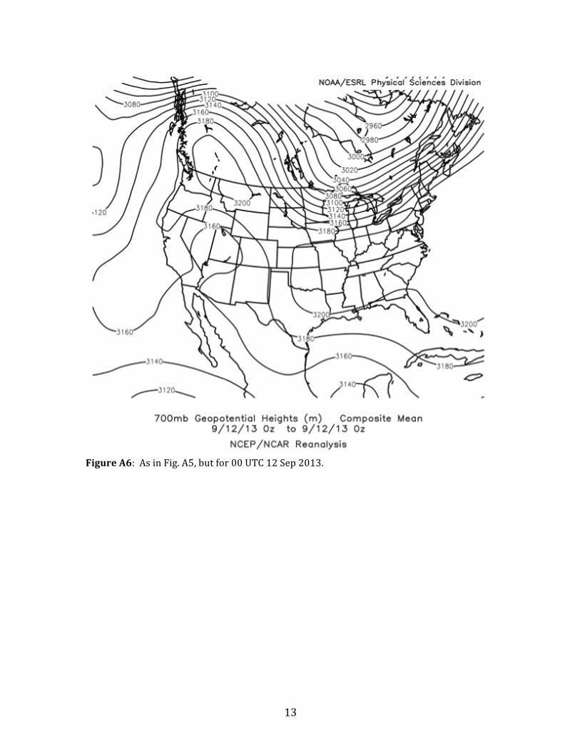
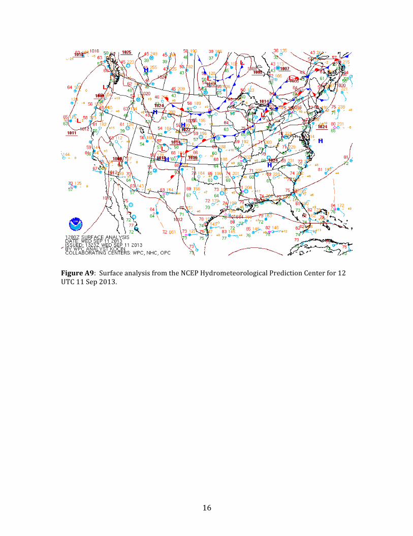
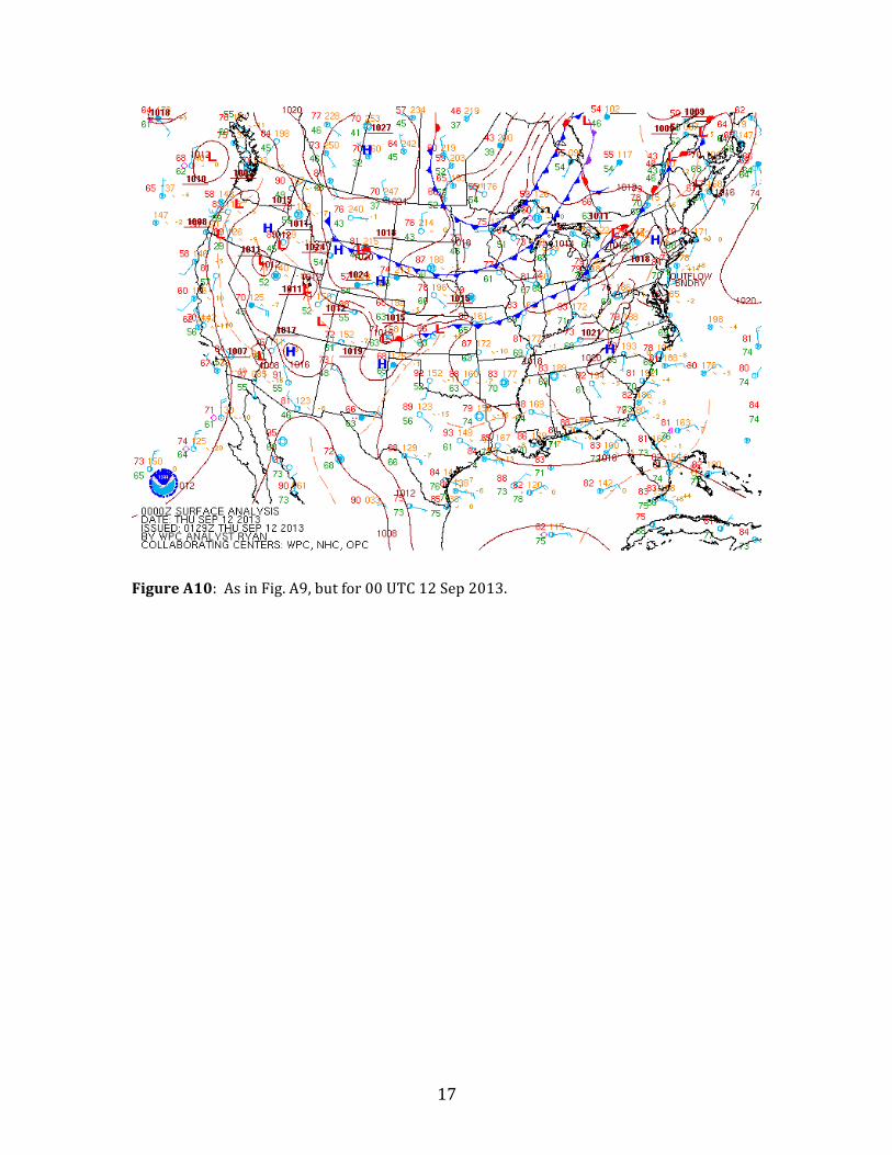
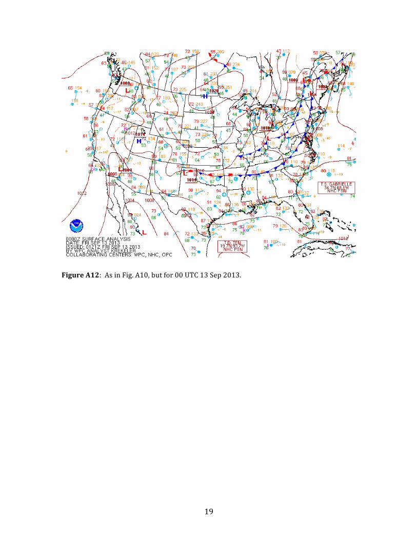
trough in the intermountain west, with sustained southerly flow at 500 hPa from the eastern Pacific, where previously tropical storm Lorena had been active. During the period of heaviest precipitation on 11-‐12 Sep 2013, the 700 hPa geopotential height pattern indicated light southeasterly flow over the northern Front Range. The surface pattern indicated a high-‐pressure system to the north that was moving slowly to the southeast. A weak front was draped to the south and east of the northern Colorado Front Range. Rawinsonde soundings at Denver, CO showed a sustained period of saturated, nearly neutral-‐stability atmospheric conditions. Global Positioning System (GPS; Gutman et al. 2004) total-‐column precipitable water measurements from Boulder indicated a sustained, multi-‐day period of record precipitable water compared to the September climatology. Figures provided below document these characteristics.

8

Figure A1: 500 hPa analyzed geopotential height pattern for 12 UTC 11 Sep 2013, as determined from the NCEP-‐NCAR reanalysis. Geopotential height is contoured every 20 m.

9

Figure A2: As in Fig. A1, but for 00 UTC 12 Sep 2013.

10


11

Figure A4: As in Fig A1, but for 00 UTC 13 Sep 2013.

12

Figure A5: As in Fig. A1, but for 700 hPa geopotential height for 12 UTC 11 Sep 2013.

13


14


15


16

Figure A9: Surface analysis from the NCEP Hydrometeorological Prediction Center for 12 UTC 11 Sep 2013.

17


18


19


20


21

Figure A14: Skew-‐T thermodynamic diagram for Denver, Colorado on 00 UTC 11 Sep 2013.

−40 −30 −20 −10 0 10 20 30 40

100

200

300

400

500

600

700

800

900

1000 0.4 1 2 4 7 10 16 24 32 40g/kg110 m

795 m

1526 m

3162 m

5880 m

7600 m

9700 m

10960 m

12420 m

14210 m

16670 mSLAT 39.75SLONSELV 1625.SHOW −9999LIFT −0.02LFTV −0.07SWET −9999KINX −9999CTOT −9999VTOT −9999TOTL −9999CAPE 77.51CAPV 94.82CINS 0.00CINV 0.00EQLV 237.4EQTV 237.0LFCT 796.3LFCV 797.5BRCH 1.32BRCV 1.61LCLT 287.0LCLP 800.2MLTH 305.9MLMR 12.64THCK 5770.PWAT 36.51

00Z 11 Sep 2013 University of Wyoming

72469 DNR Denver

22


−40 −30 −20 −10 0 10 20 30 40

100

200

300

400

500

600

700

800

900

1000 0.4 1 2 4 7 10 16 24 32 40g/kg122 m

807 m

1538 m

3171 m

5880 m

7580 m

9670 m

10930 m

12400 m

14210 m

16640 mSLAT 39.75SLONSELV 1625.SHOW −9999LIFT −0.62LFTV −0.72SWET −9999KINX −9999CTOT −9999VTOT −9999TOTL −9999CAPE 150.8CAPV 184.7CINS 0.00CINV 0.00EQLV 301.2EQTV 288.6LFCT 800.1LFCV 808.6BRCH 17.15BRCV 21.00LCLT 287.1LCLP 813.2MLTH 304.5MLMR 12.48THCK 5758.PWAT 32.97


72469 DNR Denver

23


−40 −30 −20 −10 0 10 20 30 40

100

200

300

400

500

600

700

800

900

1000 0.4 1 2 4 7 10 16 24 32 40g/kg127 m

810 m

1539 m

3175 m

5890 m

7590 m

9680 m

10940 m

12420 m

14220 m

16660 mSLAT 39.75SLONSELV 1625.SHOW −9999LIFT −1.77LFTV −2.08SWET −9999KINX −9999CTOT −9999VTOT −9999TOTL −9999CAPE 499.5CAPV 570.4CINS −0.30CINV −0.20EQLV 258.4EQTV 256.8LFCT 786.6LFCV 788.5BRCH 20.94BRCV 23.91LCLT 288.0LCLP 813.7MLTH 305.5MLMR 13.27THCK 5763.PWAT 33.16


72469 DNR Denver

24


−40 −30 −20 −10 0 10 20 30 40

100

200

300

400

500

600

700

800

900

1000 0.4 1 2 4 7 10 16 24 32 40g/kg146 m

827 m

1555 m

3186 m

5900 m

7600 m

9680 m

10940 m

12410 m

14230 m

16650 mSLAT 39.75SLONSELV 1625.SHOW −9999LIFT 0.06LFTV 0.01SWET −9999KINX −9999CTOT −9999VTOT −9999TOTL −9999CAPE 170.7CAPV 197.8CINS −12.5CINV −11.2EQLV 283.0EQTV 280.7LFCT 646.2LFCV 646.9BRCH 8.33BRCV 9.66LCLT 287.1LCLP 819.2MLTH 304.0MLMR 12.46THCK 5754.PWAT 34.25


72469 DNR Denver

25


−40 −30 −20 −10 0 10 20 30 40

100

200

300

400

500

600

700

800

900

1000 0.4 1 2 4 7 10 16 24 32 40g/kg137 m

818 m

1546 m

3179 m

5880 m

7580 m

9680 m

10930 m

12400 m

14210 m



72469 DNR Denver

26


−40 −30 −20 −10 0 10 20 30 40

100

200

300

400

500

600

700

800

900

1000 0.4 1 2 4 7 10 16 24 32 40g/kg107 m

789 m

1516 m

3145 m

5850 m

7550 m

9650 m

10900 m

12370 m

14180 m



72469 DNR Denver

27

Online appendix A references Barkmeijer, J., Buizza, R., Palmer, T. N., Puri, K. and Mahfouf, J.-‐F., 2001. Tropical singular vectors computed with linearized diabatic physics. Quart. J. Royal Meteor. Soc, 127, 685–708. Berner, J., Shutts, G. J., Leutbecher, M. and Palmer, T. N., 2009. A spectral stochastic kinetic energy backscatter scheme and its impact on flow-‐dependent predictability in the ECMWF ensemble prediction system. J. Atmos. Sci., 66, 603–626. Bowler, N.E., Arribas A., Mylne K.R., Robertson, K.B., and Beare, S.E., 2008. The MOGREPS short-‐range ensemble prediction system. Quart. J. Royal Meteor. Soc., 134, 703–722. Brown, J. D., D.-‐J. Seo, and J. Du, 2012: Verification of precipitation forecasts from NCEP’s Short-‐Range Ensemble Forecast (SREF) system with reference to ensemble streamflow prediction using lumped hydrologic models. J. Hydrometeor, 13, 808–836. doi: http://dx.doi.org/10.1175/JHM-‐D-‐11-‐036.1 Buizza, R. and Palmer, T. N. (1995). The singular vector structure of the atmosphere global circulation. J. Atmos. Sci., 52, 1434–1456. Buizza, R., Miller, M. and Palmer, T. N. (1999b). Stochastic representation of model uncertainties in the ECMWF ensemble prediction system. Quart. J. Royal Meteor. Soc., 125, 2887–2908. Clayton A. M., Lorenc, A. C., and Barker, D. M., 2013. Operational implementation of a hybrid ensemble/4D-‐Var global data assimilation system at the Met Office. Quart. J. Royal Meteor. Soc., 139, 1445–1461. DOI:10.1002/qj.2054 Du, J., G. DiMego, Z. Toth, D. Jovic, B. Zhou, J. Zhu, H. Chuang, J. Wang, H. Juang, E. Rogers, and Y. Lin, 2009: NCEP short-‐range ensemble forecast (SREF) system upgrade in 2009. 19th Conf. on Numerical Weather Prediction and 23rd Conf. on Weather Analysis and Forecasting, Omaha, Nebraska, Amer. Meteor. Soc., June 1-‐5, 2009, paper 4A.4, Available online at http://www.emc.ncep.noaa.gov/mmb/SREF/reference.html ECMWF, 2012: IFS documentation -‐-‐ Cy38r1 Operational implementation 19 June 2012, Part V: ensemble prediction system. Available at http://www.ecmwf.int/research/ifsdocs/CY38r1/IFSPart5.pdf, 25 pp. Flowerdew, J., and Bowler, N.E., 2013. On-‐line calibration of the vertical distribution of ensemble spread. Quart. J. Royal Meteor. Soc., 139, 1863–1874. DOI:10.1002/qj.2072

28

Gagnon, N., X.-‐X. Deng, P.L. Houtekamer, M. Charron, A. Erfani, S. Beauregard, B. Archambault, F. Petrucci, and A. Giguère, 2013: Improvements to the Global Ensemble Prediction System (GEPS) from version 2.0.3 to version 3.0.0. Canadian Meteorological Centre Tech Memo, available at http://collaboration.cmc.ec.gc.ca/cmc/cmoi/product_guide/docs/lib/op_systems/doc_opchanges/technote_geps300_20130213_e.pdf Gutman, S.I., S.R. Sahm, S.G. Benjamin, B.E. Schwartz, K.L. Holub, J.Q. Stewart, and T.L. Smith, 2004: Rapid retrieval and assimilation of ground based GPS precipitable water observations at the NOAA Forecast Systems Laboratory: impact on weather forecasts. J. Meteor. Soc. Japan, 82, 351-‐360.

Hamill, T. M., J. S. Whitaker, M. Fiorino, and S. J. Benjamin, 2011a: Global ensemble predictions of 2009's tropical cyclones initialized with an ensemble Kalman filter. Mon. Wea. Rev., 139, 668-‐688. doi: http://dx.doi.org/10.1175/2010MWR3456.1 Hamill, T. M., J. S. Whitaker, D. T. Kleist, M. Fiorino, and S. J. Benjamin, 2011b: Predictions of 2010's tropical cyclones using the GFS and ensemble-‐based data assimilation methods. Mon. Wea. Rev., 139, 3243-‐3247. Hou, D., Z. Toth, Y. Zhu, and W. Yang, 2008: Impact of a stochastic perturbation scheme on global ensemble forecast. Proc. 19th Conf. on Probability and Statistics, New Orleans, LA, Amer. Meteor. Soc., 1.1. [Available online athttps://ams.confex.com/ams/88Annual/techprogram/paper_134165.htm.] Isaksen, L. M. B., R. Buizza, M. F., Haseler, J., Leutbecher, M. and Raynaud, L. (2010). Ensemble of data assimilations at ECMWF. Technical Report 636, ECMWF, Reading, UK. Kleist, Daryl T., David F. Parrish, John C. Derber, Russ Treadon, Wan-‐Shu Wu, Stephen Lord, 2009: Introduction of the GSI into the NCEP Global Data Assimilation System. Wea. Forecasting, 24, 1691–1705. doi: http://dx.doi.org/10.1175/2009WAF2222201.1 Kleist, Daryl T., David F. Parrish, John C. Derber, Russ Treadon, Ronald M. Errico, Runhua Yang, 2009: Improving Incremental Balance in the GSI 3DVAR Analysis System. Mon. Wea. Rev., 137, 1046–1060. doi: http://dx.doi.org/10.1175/2008MWR2623.1 Liu, Q., T. Marchok, H.-‐L. Pan, M. Bender, and S. J. Lord, 2000: Improvements in hurricane initialization and forecasting at NCEP with global and regional (GFDL) models. NWS Tech. Procedures Bulletin 472, 7 pp. [Available online at http://www.nws.noaa.gov/om/tpb/472.htm].

29

Palmer, T. N., Buizza, R., Doblas-‐Reyes, F., Jung, T., Leutbecher, M., Shutts, G. J., Steinheimer, M. and Weisheimer, A., 2009. Stochastic parameterization and model uncertainty. ECMWF Tech. Memo. 598, 42 pp. Tennant, W.J., Shutts, G.J., Arribas, A., and Thompson, S.A., 2011. Using a stochastic kinetic energy backscatter scheme to improve MOGREPS probabilistic forecast skill. Mon. Wea. Rev., 139, 1190–1206. Toth, Z., and E. Kalnay, 1997: Ensemble forecasting at NCEP and the breeding method. Mon. Wea. Rev., 125, 3297-‐3319. Wei, M., Z. Toth, R. Wobus, and Y. Zhu, 2008: Initial perturbations based on the ensemble transform (ET) technique in the NCEP global operational forecast system. Tellus, 60A, 62–79. Zhu, K., Y. Pan, M. Xue, X. Wang, J. S. Whitaker, S. G. Benjamin, S. S. Weygandt, and M. Hu, 2013: A regional GSI-‐based ensemble Kalman filter data assimilation system for the Rapid Refresh configuration: testing at reduced resolution. Mon. Wea. Rev., 141, 4118–4139. doi: http://dx.doi.org/10.1175/MWR-‐D-‐13-‐00039.1

Performance!of!Operational!Model!PrecipitationForecast ... · PDF fileensemble!forecasts!with!their!MOGREPS!(Met!Office!Global!and!Regional!Ensemble! ......

Documents