Performance of Alternative Price Forecast for Pakistan

Forman Christian College (A Chartered University) was founded in 1864 by

Dr. Charles W. Forman, a Presbyterian missionary from USA. In 1972 the

college was nationalized by the government of Pakistan and it was returned to

the present owners of the college on March 19, 2003. In March 2004, the

government of Pakistan granted university status to Forman Christian

College.

For submission of articles for publication and purchase of Forman Journal of

Economic Studies:

Contact Editor Forman Journal of Economic Studies Department of Economics Forman Christian College (A Chartered University) Ferozepur Road, Lahore-54600, Pakistan E mail: [email protected] Ph: +92 42 99231581-8, Ext: 380 Fax: +92 42 99230703 www.fccollege.edu.pk Subscription Rate Inland

Students Rs.200 General Rs.300

Overseas US $ 40 ISSN: 1990-391X Abbreviated Key Title: Forman j. econ. stud. Recognized by: Higher Education Commission, Category-Y Internationally Indexed by: EconLit, EBSCOhostTM, IBSS & Ulrich’s Journal Website: www.fccollege.edu.pk/academics/departments/academic- departments/department-of-economics/research

i

Forman Journal of Economic Studies Patron

James A. Tebbe Editor Associate Editors Managing Editor Muhammad Aslam Chaudhary Tanvir Ahmed Ghulam Shabbir Muhammad Akbar National Advisory Board Asad Zaman International Islamic University, Islamabad Eatzaz Ahmad Quaid-i-Azam University, Islamabad Fazal Hussain PIDE, Islamabad Imran Sharif Chaudhry Bahauddin Zakariya University, Multan Khair-uz-Zaman Gomal University D. I. Khan Michael Murphy Forman Christian College University, Lahore Muhammad Aslam Lahore School of Economics, Lahore Muhammad Idrees Quaid-i-Azam University, Islamabad Mumtaz Anwar Ch. University of the Punjab, Lahore Mushtaq Ahmed Lahore University of Management Sciences, Lahore Naveed Ahmed Institute of Business Administration, Karachi Razaque H. Bhatti International Islamic University, Islamabad Shah Nawaz Malik Bahauddin Zakariya University, Multan International Advisory Board Chang Yee KWAN National University of Singapore, Singapore David Graham Institute of Defense Analysis, Alexandria, VA, USA Ismail Cole University of California, PA, USA James Fackler University of Kentucky, USA Kiyoshi Abe Hanazono, Hanamigaaku, Chiba City, Japan M. Arshad Chaudhary University of California, PA, USA Mack Ott Gravitas International LLC, USA Marwan M. El Nasser Fredonia University, USA Muhammad Ahsan Academic Research Consultant / Adviser, UK Nasim S. Sherazi Islamic Development Bank, Saudi Arabia Roger Kormendi University of Michigan, USA Sarkar Amin Uddin Fredonia University, USA Soma Ghosh Albright College, USA Stephen Ferris Carleton University, Canada Steve Margolis North Carolina State University, USA Suchandra Basu Rhode Island College, USA Toseef Azid Taibah University Madinah, Saudi Arabia Thomas Zorn University of Nebraska, USA

ii

Declaration

The findings, interpretations and conclusions expressed in this journal are

entirely those of the authors and should not be attributed in any manner to the

FCC or Editorial Board. The journal does not guarantee accuracy of the data

included in this publication and accepts no responsibility for any consequence

of their use.

iii

FORMAN JOURNAL OF ECONOMIC STUDIES

Volume: 8 2012 January-December An Analysis of International Income Inequality 1

Muhammad Idrees and Eatzaz Ahmad

Impact of Natural Disasters, Terrorism and Political News on 13 KSE-100 Index

Mian Ahmad Hanan, Saleem Noshina, Saqib Ali Siddiqui and Shahid Imran

Performance of Alternative Price Forecast for Pakistan 31 Yaser Javed and

Eatzaz Ahmad Impact of Trade Openness on Exports Growth, 63 Imports Growth and Trade Balance of Pakistan

M. Aslam Chaudhary and Baber Amin

Determinants of Youth Activities in Pakistan 83 Rizwan Ahmad and

Ijaz Hussain A Study of Implicit Tax in Pakistan’s Agriculture, with 107 Special Reference to the Case of Rice

Mohammad Aslam Determinants of Residential Electricity Expenditure in Pakistan: 127 Urban-Rural Comparison

Ijaz Hussain and Muhammad Asad

DEPARTMENT OF ECONOMICS FORMAN CHRISTIAN COLLEGE (A CHARTERED UNIVERSITY)

FEROZEPUR ROAD, LAHORE, PAKISTAN

Forman Journal of Economic Studies Vol. 8, 2012 (January–December) pp. 31-61

PPeerrffoorrmmaannccee ooff AAlltteerrnnaattiivvee PPrriiccee FFoorreeccaasstt ffoorr PPaakkiissttaann Yaser Javed and Eatzaz Ahmad1

Abstract

To evaluate the price forecasts, we use two data frequencies i.e., annual and quarter with two most demanding techniques, i.e., ARIMA and VAR models to forecast the four index of inflation, named, Consumer Price Index (CPI), Wholesale Price Index (WPI), GNP Price Deflator (GNPPD), and Implicit Price Deflator of Total Domestic Absorption (DAPD).2 In order to test the performance of price forecast for Pakistan, we found Consumer Price Index (CPI) and Implicit Price Deflator of Total Domestic Absorption (DAPD) better than Wholesale Price Index (WPI) and GNP Price Deflator (GNPPD). In general more elaborate Vector Autoregressive (VAR) models outperform the simplistic Auto Regressive Integrated Moving Average (ARIMA) models in forecasting a price series. Another useful conclusion is that the quarterly data provide better forecasts than the annual data. All these results support the econometricians’ maintained hypotheses that, data observed at high frequency and statistically more elaborate use of a given data set provides better predictions than the data observed at low frequency and analyzed with simplistic statistical tools.

Keywords: ARIMA models; Cointegration; ECM; VAR Models

JEL classification: C12, C13, C15, C22, E30, E31, E37, E58

1. Introduction Uncertainty about future events influence our present decision, the main reason why expectations are made is that we want to incorporate that uncertainty in our present decision to minimize the risk. For example, a student does not know whether it will rain in the afternoon when he/she returns from university. The student has to decide now on the basis of his/her judgment or given knowledge about the pattern of climate whether carry umbrella or leave it at home. A good decision about afternoon, in the morning is important. 1 The authors are Ph.D. Student at Federal Urdu University of Arts, Science and Technology, Islamabad and Professor/Dean at School of Economics, Quaid-i-Azam University Islamabad, respectively. 2 Total domestic absorption price deflator is obtained from addition of imports and subtraction of exports from GNP. This deflator was used by Ahmad and Ram (1991).

Javed and Ahmad

32

Macroeconomic policy makers are interested to know the inflation rates for the coming years. If these figures are alarming then they suggests monetary authorities that to tighten their steps towards monetary policy right now, so that the remedy starts before occurring of the disease. Forecasting is an important exercise in the context of time series analysis according to Yin-Wong and Menzie (1997) a large industry is involved in the forecasting of key macroeconomic variables.

None of the variable can be predict with certainty; decisions are made on the basis of forecasts made by researches are individuals, but no forecast is ever perfect there must be some errors. Importance of correct forecast is obvious, from the observation of Blix et al. (2002) that a bad forecast can lead to loss of business opportunities, loss of investment or to misguide government macroeconomic policies; good forecast, on the other hand, can lead to the opposite. So it is important to test the performance of such forecasts.

The remaining portion of the study is organized as follows. In section 2, we review the existing literature on measuring performance of price forecast and in section 3, empirical findings of the pertinent studies. In section 4, we present data sources, estimation techniques and in section 5 we present different type of performance hypothesis. In section 6, we present the results of our performance tests. Finally section 7 concludes the study.

2. Review of Literature Analysis of time series started before the evolution of modern macroeconomics, according to Yule (1927) forecasting has an even longer history. Importance of time series analysis and forecast is obvious from the observation of Ruey (2000) that objectives of the two studies may differ in some situations, but forecasting is often the goal of a time series analysis.

Forecasting of economic time series is an important but difficult task; especially in case of developing countries due to the poor quality of data, there is also persistently destabilize economic and political environment. Economics outcomes are often influenced by unanticipated events and data may be inadequate, particularly in developing countries. According to Paula (1996) economic forecasting is an art, not a science.

Granger (1996) points out that it is easy to find criticisms of economic forecasts, both of their perceived quality and of the methods used in their construction. No forecast can be properly evaluated in isolation and so it is

Performance of Alternative Price Forecast for Pakistan

33

worth noting that famous book by Box and Jenkins (1976) on univariate models, has attracted substantial opponents in forecasting competitions. According to Granger (1989) it is not possible to give a definite answer to the question like ‘What is the best forecasting method?’. In any particular forecasting situation some methods may be excluded either because of insufficient data or because the cost is too high. If there are no such limitations, it is still not possible to give a simple answer.

Importance of correct forecast is obvious, as according to Blix et al. (2002) a bad forecast can lead to loss of business opportunities3, missed investment or misguide government macroeconomic policies; good forecast, on the other hand, can lead to the opposite. Accuracy of forecast is important to policymakers, as several studies evaluate the forecasts, such as Gavin and Mandal (2000), Oller and Barot (2000) and Batchelor (2001). As mentioned Nordhaus (1987), given the heightened importance of forecasts and expectations, it is natural to inquire into their accuracy and adequacy.

2.1. Consistent Forecast Generally a forecast having lower RMSE is considered better than the ones having a higher value of RMSE. As mentioned by Yin-Wong and Menzie (1997) when examining forecast accuracy researchers examine the mean, variance and serial correlation properties of the forecast errors. The issues of integration and cointegration are rarely addressed. These issues are very important as pointed out by Clement and Hendry (1993) and Armstrong and Fildes (1995) make a criticism on the RMSE, and mention that RMSE is not a good benchmark.

After the rejection of conventional tools of analyzing the forecast, the cointegration approach named ‘consistency’ was introduced, and this technique was also used by Liu and Maddala (1992) and Aggarwal et al. (1995) to assess the unbiasedness, integration and cointegration characteristics of macroeconomic data and their forecasts.

2.2. Efficient Forecast Efficiency norm is defined by different researchers, and in different ways. In a Congressional Budget Office Report (1999) efficiency indicates the extent to which a particular forecast could have been improved by using

3 The expectations of the businessmen and investors play a key role in the business cycles theories presented by Pigou (1927) and Keynes (1936).

Javed and Ahmad

34

additional information that was at the forecaster’s disposal when the forecast was made. Nordhaus (1987) define efficiency in two ways i.e., ‘weak’4 and ‘strong’ efficiency. This kind of efficiency states by Beach et al. (1999).

Bonham and Cohen (1995) criticize the methodology used by Keane and Runkle (1990) that directly tests conditional efficiency of forecast using an approach that based on incorrect integration accounting. Their integrating accounting errors result in trivial cointegration and improper distributional assumption and, therefore, incorrect inference. Bonham and Cohen (1995) claim that they correct the integration accounting errors and show that the efficiency hypothesis is still rejected.5

2.3. Rational Forecast Doctrine of rationality is defined by Lee (1991) as follows, expectations are said to be rational if they fully incorporate all of the information available to the agents at the time the forecast is made. There are many studies like Hafer and Hein (1985), McNees (1986), Pearce (1987) and Zarnowitz (1984 and 1985) that places great weight on minimum mean square error (MSE) but do not incorporate accuracy analysis convincingly in their tests of rationality. However, there are many studies like Holden et al. (1987), Ash (1990 and 1998), Artis (1996), Pons (1999, 2000 and 2001), Kreinin (2000), Oller and Barot (2000) and Batchelor (2001), shows that the IMF and OECD forecasts pass most of the tests of rationality.

Rather than simply compare forecast on the basis of RMSE, Bonham and Douglas (1991) include a test for conditional efficiency6 in the definition of strong rationality. In order to analyze the rationality of price forecast Bonham and Douglas (1991) define a hierarchy of rationality tests starting from ‘weak rationality’ to ‘strict rationality’. The level of rationality in hierarchy is defined as, weak, sufficient, strong and strict.

4 Another notion of efficiency proposed by Bakhshi et al. (2003) is that current forecast errors should be uncorrelated with past forecast. 5 In this study we are not much concern with the colliding debate of efficiency related to Bonham and Cohen (1995) and Keane and Runkle (1990, 1994 and 1995) due to some flaws with respect to comparative analysis between the forecasts obtained from ARIMA and VAR models. 6 Granger and Newbold (1973), describe conditional efficiency as a forecast for which the combination forecast does not produce a lower RMSE than its component forecast.


35

2.3.1. Weak Rationality Most of the applied work such as Evans and Gulmani (1984), Friedman (1980), Pearce (1987) and Zarnowitz (1984 and 1985) view rationality in term of the necessary conditions of unbiasedness and information efficiency.7 According to the notion of weak rationality defines by Bonham and Douglas (1991), the forecast must be unbiased and meet the tests of weak information efficiency.

Ruoss and Marcel (2002) state that unbiasedness is often tested using the Theil-Mincer-Zarnowitz equation. This is a regression of the actual values on a constant and the forecast values. The null hypothesis to be tested is that, the intercept is equal to zero and the slope is equal to one. Holden and Peel (1990) pointed out that this null hypothesis is merely sufficient but not necessary for unbiasedness. Clement and Hendry (1998) suggest, running a regression of the forecast error on the constant, if the parameter estimate deviates from zero, the hypothesis that the forecast is unbiased is rejected.

2.3.2. Sufficient Rationality The forecast must be weak rational and must pass a more demanding test of sufficient orthogonality, namely, that the forecast errors is uncorrelated with any variable in the information set available at the time of prediction.

Rational expectation hypothesis played a critical role in macroeconomic analysis and in the theory of economics decision-making. Rational expectation assumes that economic agents are rational optimizers, especially in making forecasts and in taking actions based on such forecasts. Rational expectations hypothesis by Muth (1961) holds that predictions of future inflation are formed in a manner that fully reflects relevant information currently available.

2.3.3. Strong Rationality The forecast must be sufficiently rational and pass tests of conditional efficiency. Conditional efficiency requires a comparison of forecasts.8 Consider a sufficiently rational forecast as a benchmark. Combine benchmark 7 The same kind of unbiasedness and efficiency notion was build by Eichenbaum et al. (1988) and Razzak (1997). 8 Started from the classic study of Bates and Granger (1969), a large literature on forecast combination summarized by Clemen (1989), Diebold and Jose (1996) and Timmermann (2005) has found evidence that combined forecasts tend to produce better forecast than individual forecasting models.

Javed and Ahmad

36

with some competing forecast. Conditional efficiency refers to Granger and Newbold (1973) that measures the reduction in RMSE, which occurs when a forecast is combined with one of its competitors. Against such kind of notion Granger (1989) suggest that combining often produces a forecast superior to both components. Same kind of notion is build by Timmermann (2006). If the combination produces an RMSE that is significantly smaller than the benchmark RMSE, the benchmark forecast fails the test for conditional efficiency because it has not efficiently utilize some information contained in the competing forecast. Stock and Mark (2001) report broad support for a simple combination of forecasts in a study of a large cross-section of macroeconomic and financial variables.

2.3.4. Strict Rationality According to Bonham and Douglas (1991) a statement about rationality should not depend on arbitrary selection of time periods. A forecast is strictly rational if it passes tests of strong rationality in a variety of sub-periods, stated in section 5.3.4.

3. Empirical Findings Yin-Wong and Menzie (1997) concludes that the (final) Treasury bill rate, housing starts, industrial production, inflation and most of their respective forecasts appear to be trend stationary. The corporate bond rate, GNP, the GNP deflator, unemployment and most of their respective forecasts appear to be difference stationary. About half of the unit root pairs are cointegrated. In only one of these cases the unitary elasticity restriction is rejected the 1-quarter ahead GNP deflator forecast. In the study of Yin-Wong and Menzie (1997) 30 out of 36 cases fulfill the requirement that forecast and actual series possess the same order of integration. Surprisingly, the linkage between forecasts and unrevised actual series is not unambiguously stronger. However, while there is more evidence of cointegration, there is also a greater rate of rejection of the unitary elasticity restriction.

The evidence from the study of Aggerwal et al. (1995) indicate that there are significant deviations from the rational expectations hypothesis for survey forecasts of a number of macroeconomics series. They find that survey forecasts for the consumer price index and personal income are stationary and consistent with the rational expectation hypothesis and that the surveys of housing starts, the unemployment rate and the trade balance are rational forecasts in the sense that the announced values and their survey


37

forecasts are cointegrated. Aggerwal et al. (1995) suggests, that the quality of forecast of industrial production and retail sales can be improved significantly by using past values. These results have important implications for decisions by many economic agents and for research based on these survey forecasts and also favoring the univaraite methodology.

Results of weak efficiency hypothesis stated by Nordhaus (1987) are that 50 of 51 tests, the forecast were found to be positively correlated. The degree of correlation appears to be highest for institutional forecasts (such as those made by international agencies) and lowest for professional forecasters using time-series techniques. Nordhaus (1987) describes two reasons for this kind of inefficiency. First, perhaps the true forecasts are indeed efficient, while the published forecasts are not. Second, surely the high degree of forecast inefficiency of international institutions must contain some element of bureaucratically based forecast inefficiency.

Empirical results regarding the rationality of forecasts was explained by Lee (1991) that forecast is fail to be rational in the strong sense even though they are not rejected by the conventional test of weak rationality. Ruoss and Marcel (2002) examine the forecast rationality of the Swiss economy says that GDP forecasts in our sample do not pass the most stringent test i.e., the test of strong informational efficiency, because, in some cases, forecasts errors correlate with the forecasts of the other institutes.

Same kind of results is shown by Bonham and Douglas (1991) that the most stringent criteria for testing rationality will not be useful for empirical work. On these criteria there might not be a rational forecast of inflation. Bonham and Douglas (1991) states that, rational forecast is getting by relaxing the criterion that defines strict rationality.

Razzak (1997) and Rich (1989) test the rationality of National Bank of New Zealand’s survey data of inflation expectation and SRC expected price change data respectively. Both studies end up with a same conclusion, that the results do not reject the null hypothesis of unbiasedness, efficiency and orthogonality for a sample from their particular survey data series.

4. Data Sources and Forecast Modeling

In order to test the performance of price forecast for Pakistan, we forecast four proxies of prices, namely, Consumer Price Index (CPI), Wholesale Price Index (WPI), GNP Price Deflator (GNPPD) and Implicit Price Deflator of Total Domestic Absorption (DAPD). Annual data is taken from

Javed and Ahmad

38

various issues of Economic Survey of the Ministry of Finance, Government of Pakistan, and Annual Reports of State Bank of Pakistan. Quarterly data is taken from the IMF’s International Financial Statistics (2005) and World Bank’s World Development Indicator (2006). Data of quarter GDP is taken from the research paper of Kemal and Arby (2001). Data is taken on annual and quarter basis for the period from 1972-73 to 2004-05 and 1972Q2 to 2005Q2, respectively.

For a better forecast, our estimation is based on univariate and multivariate techniques. For the univariate technique, we use the Box-Jenkins approach to modeling ARIMA models (Box and Jenkins, 1976). For the multivariate technique, we use VAR approach presented by Sims (1980). In the estimation of VAR we use price variable alternatively with the four other variables, real GDP, Broad Money (M2), interest rate and exchange rate.

After three stages of identification, estimation and diagnostic checking, we present the specification of ARIMA models in table 4.1. In table 4.2, we present the lag specification of VAR models.

Table 4.1: Specification of ARIMA Models

Annual Data Consumer Price Index ARIMA (1,1,1) Wholesale Price Index ARIMA (0,1,1) GNP Price Deflator ARIMA (0,1,1) Domestic Absorption PD ARIMA (0,1,1)

Quarterly Data Consumer Price Index ARIMA (0,1,0) Wholesale Price Index ARIMA (4,1,0) GNP Price Deflator ARIMA (4,1,4) Domestic Absorption PD ARIMA (4,1,4)

Note: ARIMA (p,d,q) stands for a model with autoregressive process of order p and moving average process of order q applied to data integrated of order d.

Table 4.2: Specification of VAR Models

Annual Data Consumer Price Index Wholesale Price Index

VAR (1) VAR (1)

GNP Price Deflator VAR (1) Domestic Absorption PD VAR (1)

Quarterly Data Consumer Price Index VAR (1,2) Wholesale Price Index VAR (1,4) GNP Price Deflator VAR (1,2,4) Domestic Absorption PD VAR (1,4)

Note: The number in brackets show the lag periods specified in the VAR models.


39

5. Performance Hypothesis After getting the forecasts we test the performance of price forecasts by applying the different type of hypothesis under the definition of consistency, efficiency and rationality.

5.1. Consistency Test of Forecast Consistent forecast states that the, observed price index and their relevant forecast series are integrated of same order and they are cointegrated. To test the existence of unit root we follow the spirit of Dickey and Fuller (1979, 1981). According to them if yt follows AR(p) process.

tptpttt yyyy εφφφ ++++= −−− .......2211 , a series yt is said to be

stationary, if the value of ∑=

p

ii

1

φ is less than unity. If the observed variable and

their forecast are of same level of integration, say I(1). Then the first condition for consistency is met. Concept of cointegration was first introduced by Granger (1981) and elaborates further by Engle and Granger (1987). The spirit of the cointegration in this study is that observed price index (Po) is cointegrated with their forecast (Pe). Both series posses same order of integration, say I(1), then the linear combination9 of these two must be I(0). We define it in following way.

tto

te PP ε+Φ+Φ= 21 )0(It ≈ε (1)

Where { }21,ΦΦ is the cointegrating vector producing a linear combination of{ }to

te PP , , which is stationary. This will complete the proposition of

cointegration. After that there is a need to test the stability of long run relationship through error correction models.

5.1.1. Error Correction Models For the Error correction we estimate the following equations.

t

m

iit

eitt

e uPP +∆++=∆ ∑=

−−1

121 δεαα (2)

t

n

iit

oitt

o vPP +∆++=∆ ∑=

−−1

121 γεββ (3)

9 We will apply Granger Causality test presented by Granger (1969), to determine dependent variable in the linear combination of observed price series with their forecast series.

Javed and Ahmad

40

The selection of m and n in equation 2 and 3 depends on the significance of lags under t-statistics. For a stable long run relationship between observed price index with forecast the following feedback effect must be less than zero, that is.

0222 <Φ− βα (4)

If the above condition holds, it implies that disequilibrium in previous period leads to adjustment in current time period, which counter balance the disequilibrium forces.

5.2. Efficiency Test of Forecast Nordhaus (1987) define efficiency in the two classifications; weak efficiency is the necessary condition for strong efficiency, but clearly not the sufficient condition.

5.2.1 Weak Efficiency

A forecast is weakly efficient if it minimizes ( ) }{ 2t tu JΕ , where Jt is

the set of all past forecasts. Where Ut2 is the square of forecast error at time t.

In order to test weak efficiency of forecasts obtained from both techniques, we estimate the following regression.

t

k

iit

eiot PU εαα ++= ∑

=

−

1

2 (5)

Selection of k depends upon the significance under t-statistics. Only significant lags of expected price forecasts are included. Under this kind of efficiency norm, a forecast is said to be weak efficient if we are unable to reject the null that all the coefficients are simultaneously equal to zero.

5.2.2. Strong Efficiency

A forecast is strongly efficient if ( ){ }2t tu IΕ is minimized, where It is

all information available at time t. Strong efficiency requires that the square of forecast error was not explained by the information set available at time t. The information set in Univariate analysis is the past values of the variable itself, so we regress the following equation, to test the strong efficiency for the forecasts obtained from ARIMA models.


41

t

n

jit

ojot PU εαα ++= ∑

=

−

1

2 (6)

Here Pot is the observed value of price variable at time t. A forecast fails to

pass the strong efficiency hypothesis if α0 and αj are significantly different from zero. In order to test the strong efficiency of forecasts obtained from VAR we estimate the following regression.

tttttto

ot ERRMRGDPPU εαααααα ++++++= −−−−− 15141312112 2 (7)

A strongly efficient forecast obtained from VAR fail to reject the null hypothesis that all the coefficients in equation 7 are simultaneously equal to zero.

5.3. Rationality Test of Forecast Bonham and Douglas (1991) define a hierarchy of rationality tests starts from ‘weak rationality’ to ‘strict rationality’ the level of hierarchy define as follows:

5.3.1 Hypothesis of Weak Rationality A forecast must be unbiased and meet tests of weak information efficiency. Condition of unbiasedness and weak informational efficiency is set after the estimation of following equation.

tte

oto PP εαα ++= 1 (11)

A forecast is said to be unbiased if it satisfies the following conditions.

1. In equation 11, εt is serially uncorrelated.

2. In equation 11, αo and α1 are insignificantly different from zero and one respectively.

Weak information efficiency means that the forecast errors to

te

t PPE −= are uncorrelated with the past values of the predicted variables. To test the weak efficiency hypothesis we estimate the following regression equation.

t

m

iit

oiot PE εαα ++= ∑

=

−

1 (12)

Javed and Ahmad

42

If we fail to reject the following joint null hypothesis it implies that forecast errors are systematically different from zero and/or past values of the observed price series help to explain the forecast errors.

0: == jooH αα For all j = 1……….. m (13)

Acceptance of such hypothesis represent that the forecast error at time t is independent to the past information contained by relevant observed price index.

5.3.2. Hypothesis Sufficient Rationality The sufficient rationality requires that the forecast errors are not correlated with any variable in the information set available at the time of forecast. If Zt is a variable or a vector of variables used to build our forecast model, then Zt is the exogenous variable in the following equation.

t

m

iitiot ZE εαα ++= ∑

=−

1 (14)

Forecasts of ARIMA models have included only the lags of observed series as the information set. For ARIMA forecasts two lags of associated price index are used as information set. While forecasts obtained from VAR models depend upon the lags of price variables, real GDP, M2, interest rate, and exchange rate, so their lags with relevant price series are used to test sufficient rationality. After estimating the equation 14 we test the following null hypothesis.

0: == jooH αα For all j = 1……….. m (15)

The rejection of above mentioned hypothesis states that the information contained in the past values of related price series, real GDP, M2, interest rate and exchange rate, has not been used efficiently in forming the forecast.

5.3.3. Hypothesis of Strong Rationality A forecast is said to be strongly rational if it passes the test of conditional efficiency introduced by Granger et al. (1973). Conditional efficiency requires a comparison of forecasts. Call some sufficiently rational forecast as benchmark; combine the benchmark with some competing forecast. Estimate the following regression.

[ ] tttt SSD εβα +−+= (16)


43

Where Dt and St are the difference and the sum of the benchmark and combination forecast errors, respectively, and tS is the mean of the sum. Under the null hypothesis of conditional efficiency (α=β=0) the combination does not produce a lower RMSE. F test is appropriate if β>0 and the mean errors of both forecasts have the same sign as α. If the mean errors of the two forecasts do not have the same sign, then α cannot be interpret as an indicator of the relative bias of the two forecasts.

5.3.4. Hypothesis of Strict Rationality A forecast is strictly rational if it passes tests of strong rationality in a variety of sub-periods. In this study only quarter forecasts of CPI can be treated for strong efficient criterion, annual data do not have sufficient number of observation to sub-divide in various sub-periods, so we estimate equation 16 in the sub-periods;1972-Q3 to1982-Q4, 1983-Q1 to 1994-Q2 and 1994-Q3 to 2005-Q2.

If a strongly rational forecast pass the same test based on equation 16 in sub-periods mentioned above then according to Bonham and Douglas (1991) that particular forecast is awarded as strict rational.

6. Results and Discussion We are not going to discuss the conventional tools for analyzing the performance of forecasts, as lower RMSE and the maximum value of covariance proportion etc. as Clement and Hendry (1993), Armstrong et al. (1995) make a criticism on the RMSE, and mention that RMSE is not a good benchmark. In general, we can say that forecast of Consumer Price Index (CPI) is the best (among the others proxies of price variables used in this study), while the forecasts of Wholesale Price Index (WPI) are not performing well with reference to consistency, efficiency and rationality tests, because forecasts from VAR models are not able to meet the tests of weak and strong efficiency except for the quarterly CPI forecast that significantly accept the weak efficiency hypothesis.

6.1. Results of Consistency Tests of Forecast As an initial condition of consistency, observed and expected price variables should be the same order of integration. The results of unit root tests of observed data series are given in table 6.1.1.

It is obvious from the results given in table 6.1 that the four price series included in this study have unit root at levels form. Other variables also

Javed and Ahmad

44

have unit root except the annual series of interest rate that is stationary at level. One variable i.e., WPI is stationary at 10% level of significant. But following the general practice of considering the level of significant at 5%, we conclude that all the annual and quarter observed data series except the annual interest rate series are I(1). Simply the four annual and four quarter price series are I(1), then in order to satisfies the conditions of consistency the forecasts series must be I(1). The results of unit root test for the ARIMA and VAR forecasts are shown in table 6.1.2 and 6.1.3 respectively.

The results in these tables shows that all the forecasts series obtained in this study are I(1). For consistency the second condition is that the observed price series must be cointegrated with their respective forecast. In this study find the evidence on cointegration between observed

Table 6.1.1: Unit Root Tests of Observed Variables

Variables t-values (Annual Data) t-values (Quarterly Data)

Level First Diff. Level First Diff. Consumer Price Index -1.38 -4.71*** -1.53 -10.28*** Wholesale Price Index -0.79 -4.93*** -2.87* -8.54*** GNP Price Deflator -1.46 -4.04*** -1.72 -10.07*** Domestic Absorption Price Deflator

-1.18 -4.27*** -1.39 -10.54***

Real GDP -0.80 -8.45*** -0.98 -21.02*** Interest Rate -3.66*** ------ -1.97 -10.13*** Exchange Rate 0.45 -5.26*** 0.98 -11.81*** M2 -0.39 -4.20*** -0.18 -18.23***

* Significant at 10% level of Significance and *** Significant at 1% level of significance.

Table 6.1.2: Unit Root Test of Forecasts from ARIMA Models

Variables t-values (Annual Data) t-values (Quarterly Data)

Level First Diff. Level First Diff. Consumer Price Index -0.35 -5.12*** -1.37 -10.35*** Wholesale Price Index -2.15 -7.64*** -1.72 -10.98*** GNP Price Deflator -0.89 -3.87*** -1.18 -10.05*** Domestic Absorption Price Deflator

-0.81 -4.34*** -0.90 -10.50***

*** Significant at 1% level of significance.

price series and their relevant forecasts, we first used Granger Causality test to determine dependent variable in the linear combination of forecast and actual


45

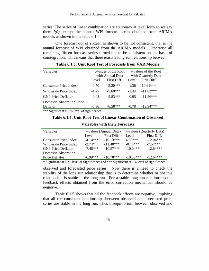
series. The series of linear combination are stationary at level form so we say them I(0), except the annual WPI forecast series obtained from ARIMA models as shown in the table 6.1.4.

One forecast out of sixteen is shown to be not consistent, that is the annual forecast of WPI obtained from the ARIMA models. Otherwise all remaining fifteen forecast series turned out to be consistent on the basis of cointegration. This means that there exists a long-run relationship between

Table 6.1.3: Unit Root Test of Forecasts from VAR Models

Variables t-values of the Root with Annual Data

t-values of the Root with Quarterly Data

Level First Diff. Level First Diff. Consumer Price Index -0.70 -5.20*** -1.36 -10.61*** Wholesale Price Index -1.27 -5.68*** -1.44 -11.82*** GNP Price Deflator -0.43 -5.83*** -0.95 -11.56*** Domestic Absorption Price Deflator

-0.36

-6.58***

-0.78

-12.94***


Table 6.1.4: Unit Root Test of Linear Combination of Observed

Variables with their Forecasts

Variables t-values (Annual Data) t-values (Quarterly Data) Level First Diff. Level First Diff.

Consumer Price Index -4.14*** -10.13*** 4.58*** -12.04*** Wholesale Price Index -2.74* -11.40*** -8.48*** -7.57*** GNP Price Deflator -7.48*** -10.57*** -10.04*** -12.84*** Domestic Absorption Price Deflator

-6.99***

-10.78***

-10.55***

-12.64***

* Significant at 10% level of Significance and *** Significant at 1% level of significance.

observed and forecasted price series. Now there is a need to check the stability of the long run relationship that is to determine whether or not this relationship is stable in the long run. For a stable long run relationship the feedback effects obtained from the error correction mechanism should be negative.

Table 6.1.5 shows that all the feedback effects are negative, implying that all the consistent relationships between observed and forecasted price series are stable in the long run. Thus disequilibrium between observed and

Javed and Ahmad

46

expected series in any period is eliminated in the subsequent period. In short, we can say that we found fifteen out of sixteen forecast series consistent and having a stable consistent long-run relationship with their relevant observed price series.

Table 6.1.5: Feedback Effects10 of Forecasts

ARIMA VAR

Annual Data Consumer Price Index -1.604 -1.458 Wholesale Price Index -2.279 -2.664 GNP Price Deflator -2.524 -3.857 Domestic Absorption PD -2.442 -3.936

Quarterly Data Consumer Price Index -1.816 -1.564 Wholesale Price Index -1.865 -1.732 GNP Price Deflator -1.659 -1.755 Domestic Absorption PD -1.626 -1.511

6.2. Results of Efficiency Tests of Forecast In the debate of efficiency we present the results of weak efficiency, the concept represents by Nordhaus (1987) as a necessary but not the sufficient condition for strong efficiency. Tables 6.2.1 and 6.2.2 represent the results of weak efficiency of annual forecasts obtained from

Table 6.2.1: Weak Efficiency of Annual Forecasts (ARIMA Models)

t

k

iit


=

−

1

2 Ho: All the coefficients are equal to zero

Equation α0 α1 α2 χ2 for Ho F-stat. for Ho CPI

Equation 9.39

(-0.98) -0.023 (-0.15)

----------- 3.002 (0.22)

1.501 (0.24)

WPI Equation

-2.11 (-0.56)

-2.00 (-3.71)***

2.35 (4.12)***

35.89 (0.00)***

11.966 (0.00)***

GNPPD Equation

-16.62 (-1.08)

-9.821 (-2.79)***

11.42 (3.07)***

24.72 (0.00)***

8.239 (0.00)***

DAPD Equation

-15.61 (-1.03)

-11.03 (-3.21)***

12.72 (3.48)***

25.398 (0.00)***

8.466 (0.00)***

Notes: t-statistics are in parentheses under the coefficients. Probabilities are in parentheses under the test statistics. *** Significant at 1% level of significance. 10 We calculate the feedback effects using Engle and Granger (1987), procedure are defined in section 5.1.1.


47

ARIMA models and VAR models respectively. Annual forecasts obtained from ARIMA are not good on the basis of weak efficiency test, except the forecast of CPI. Results reported in the table 7 shows that only the CPI forecast is weak efficient. Table 8 shows that the situation is worse for those annual forecasts we obtained from VAR, where not a single forecast series is able to pass the test of weak efficiency.

Table 6.2.2: Weak Efficiency of Annual Forecasts (VAR Models)

t

k

iit


=

−

1

2 Ho: All the coefficients are equal to zero.

Equation α0 α1 χ2 for Ho F-stat. for Ho

CPI Equation

3.04 (0.485)

0.09 (0.884)

7.18 (0.03)**

3.59 (0.04)**

WPI Equation

-0.69 (-0.613)

0.07 (3.549)***

29.38 (0.00)***

14.69 (0.00)***

GNPPD Equation

-18.43 (-2.135)**

0.65 (4.084)***

21.54 (0.00)***

10.77 (0.00)***

DAPD Equation

-15.78 (-2.220)**

0.57 (4.336)***

24.39 (0.00)***

12.2 (0.00)***

*** Significant at 1% level of significance. ** Significant at 5% level of significance.

Results presented in table 6.2.3 shows that the quarterly forecast of WPI obtained from ARIMA models is not a weak efficient forecast, while forecasts of CPI, GNPPD and DAPD accept the weak efficiency hypothesis.

Table 6.2.3: Weak Efficiency of Quarter Forecasts (ARIMA Models)

t

k

iit


=

−

1



CPI Equation

383.41 (1.06)

-0.14 (-0.33)

2.33 (0.31)

1.16 (0.32)

WPI Equation

-99.61 (-1.40)

0.41 (5.43)***

57.58 (0.00)***

28.79 (0.00)***

GNPPD Equation

0.24 (-0.77)

0.04 (1.82)*

4.72 (0.09)*

2.36 (0.10)*

DAPD Equation

-0.25 (-0.79)

0.04 (1.92)*

5.26 (0.07)*

2.63 (0.08)*

*** Significant at 1% level of significance. * Significant at 10% level of significance.

Javed and Ahmad

48

Table 6.2.4: Weak Efficiency of Quarter Forecasts (VAR Models)

t

k

iit


=

−

1



CPI Equation

361.73 (1.13)

-0.10 (-0.26)

3.11 (0.21)

1.55 (0.22)

WPI Equation

-116.39 (-1.69)*

0.46 (6.13)***

71.42 (0.00)***

35.71 (0.00)***

GNPPD Equation

-0.26 (-0.9)

0.042 (2.03)**

5.70 (0.06)*

2.85 (0.06)*

DAPD Equation

-0.27 (-0.88)

0.05 (2.10)**

6.29 (0.04)**

3.14 (0.05)**

*** Significant at 1% level of significance. ** Significant at 5% level of significance. * Significant at10% level of significance.

Quarter forecasts of GNPPD from both techniques are passing the test of weak efficiency. These results are seems to be coherent with the Nordhaus (1987), as they also find a few week efficient forecasts. After describing the results of weak efficiency, we now present the results of strong efficiency test.

Table 6.2.5: Strong Efficiency of Annual Forecasts (ARIMA Models)

t

k

iit

oiot PU εαα ++= ∑

=

−

1



CPI Equation

8.21 (0.91)

-0.005 (-0.04)

3.00 (0.22)

1.50 (0.24)

WPI Equation

-4.13 (-0.98)

0.21 (2.92)***

13.98 (0.00)***

6.99 (0.00)***

GNPPD Equation

-22.72 (-1.51)

0.91 (3.16)***

13.14 (0.00)***

6.57 (0.00)***

DAPD Equation

-19.66 (-1.26)

0.82 (2.78)***

10.32 (0.00)***

5.16 (0.01)***


Results of strong efficiency presented in table 6.2.5, indicate that from annual forecast computed by ARIMA models, no index passes the test of strong efficiency except the forecast of CPI. The results of strong efficiency reported in table 6.2.6 shows that quarter forecasts of CPI, GNPPD and DAPD all pass the test of strong efficiency whereas the WPI forecast does not


49

pass the test. We are not stating the results of strong efficiency of annual and quarter forecasts, obtained from VAR models. These results show that neither annual nor quarter forecast pass the test of strong efficiency.

Table 6.2.6: Strong Efficiency of Quarter Forecasts ARIMA Models

t

k

iit

oiot PU εαα ++= ∑

=

−

1


Equation α0 α1 χ2 for Ho F-stat. for Ho CPI

Equation 372.04 (1.40)

-0.13 (-0.31)

2.31 (0.31)

1.16 (0.32)

WPI Equation

-103.42 (-1.47)

0.42 (5.55)***

59.08 (0.00)***

29.54 (0.00)***

GNPPD Equation

-0.22 (-0.72)

0.04 (0.766)*

4.53 (0.10)*

2.27 (0.11)

DAPD Equation

-0.23 (-0.73)

0.04 (1.862)*

5.05 (0.08)*

2.52 (0.08)*

*** Significant at 1% level of significance. * Significant at10% level of significance.

6.3. Results of Rationality Tests of Forecast In this section we discuss the results of the rationality tests of forecast we get from ARIMA and VAR models. We estimate a hierarchy of rationality tests starting from ‘weak rationality’ to ‘strict rationality’ presented by Bonham and Douglas (1991).

In table 6.3.1 we present the results of weak rationality of ARIMA forecast, which was the combination of unbiasedness and weak informational efficiency present in the top panel. Where the first regression equation is the famous Theil-Mincer-Zarnowitz equation. This is a regression of the observed series on a constant and the forecast series, and their regression residuals must be serially uncorrelated to fulfill the condition of unbiasedness as well as fail to rejecting the null presented in front of first equation and the second equation represents the weak informational efficiency, if the null in front of that equation is accepted.

According to the results of weak rationality, the forecast of CPI and DAPD pass this test in both time frequencies. Quarter forecast of GNPPD also passes the test of weak efficiency, but annual forecast of GNPPD is found to be biased. Annual forecast of WPI is biased and the null hypothesis of weak informational efficiency is rejected. On the other hand the quarter forecast of WPI is found weak efficient as shown in table 6.3.1.

Javed and Ahmad

50

Here we find the same kind of evidence about the forecasts of CPI and DAPD as we result out in efficiency analysis, that these two series are better than WPI and GNPPD. Annual and quarter forecasts of CPI and DAPD are pass the two sets of tests for the rationality, therefore ARIMA models for the two indices produce rational forecasts. Annual forecast of WPI fails in both tests, while quarter forecast amazingly passes both the conditions for rationality. This is the major breakthrough of this research, because according to Bonham and Douglas (1991), Lee (1991) and Ruoss and Marcel (2002), many of the forecasts were not able to pass these tests of rationality. In table 6.3.2 we present the same set of test applied on those forecasts obtained from VAR model. There exist some similarities between results stated in table 6.3.1 and 6.3.2.

If we summarize the results of weak rationality tests of ARIMA forecasts, we find that quarter forecasts pass the both tests, annual forecasts of CPI and DAPD also passes both tests, while forecast of GNPPD is biased, but it passes the weak informational efficiency hypothesis. Quarter forecasts obtained from VAR models are found to be weakly rational, except the forecast of WPI that is biased forecast. Forecasts of CPI from annual and quarter data frequencies pass both the tests. Annual forecasts of WPI, GNPPD and DAPD are biased, but they pass the test of weak informational efficiency.

This is a hierarchy of rationality test, so we apply sufficient rationality test, to those forecast series that pass both weak informational efficiency and unbiasedness test, which are required for the weak rationality. The results of sufficient rationality test are shown in table 6.3.3 indicate that the annual forecast of CPI and DAPD obtained from ARIMA are able to pass the test of sufficient rationality. Quarter forecast of GNPPD and WPI obtained from ARIMA models passes this test of sufficient rationality. Annual and quarter forecasts of CPI obtained from VAR are sufficiently rational, while quarterly forecasts of GNPPD and DAPD do not pass the sufficient rationality test.

Strong efficiency depends on the concept presented by Granger and Newbold (1973), requiring that a forecast is combined with one of its competing forecast and the combination forecast does not produce a lower RMSE. If we look at the quarter forecasts the WPI forecast obtained from VAR is not found to be as weakly rational, GNPPD and DAPD forecasts do not posses the same signs of mean forecast error, only one forecast i.e.,


51

Table 6.3.1: Weak Rationality Tests of Forecasts (ARIMA Models)

tte

oto PP εαα ++= 1 (HoA: α0 = 0, α1 = 1)

t

m

iit


=

−

1

(oB: α0 = αj = 0)

Dependent Variable

Data Frequency

α0 α1 F-stat. (Ser. Corr.)

Null Hypothesis

χ2 for Ho

F-stat. (Ho)

CPI Annual 0.19 (0.19)

1.00 (61.02)***

1.31 (0.26)

HoA 0.22

(0.89) 0.11

(0.89) Forecast

Errors of CPI Annual -0.19

(-0.19) -0.00

(-0.05) Ho

B 0.22 (0.89)

0.11 (0.89)

CPI Quarter 0.42 (0.15)

1.00 (302.3)***

1.42 (0.24)

HoA 0.47

(0.79) 0.23

(0.79) Forecast

Errors of CPI Quarter -0.43

(-0.15) -7.2e-04 (-0.21)

HoB 0.47

(0.79) 0.23

(0.79) WPI Annual 0.81

(1.19) 0.97

(89.2)*** 9.29

(0.00)*** Ho

A 6.73 (0.03)**

3.36 (0.05)**

Forecast Errors of WPI

Annual -0.73 (-1.08)

0.02 (2.18)**

HoB 6.11

(0.05)** 3.06

(0.06)* WPI Quarter 2.88

(1.29) 0.99

(418.5)*** 0.07

(0.792) Ho

A 5.17 (0.07)*

2.58 (0.08)*


Quarter -2.85 (-1.28)

0.005 (2.12)**

HoB 5.13

(0.08)* 2.56

(0.08)* GNPPD Annual 0.42

(0.35) 0.99

(47.54)*** 4.49

(0.04)** Ho

A 0.48 (0.786)

0.24 (0.79)

Forecast Errors of GNPPD

Annual -0.32 (-0.26)

0.01 (0.533)

HoB 0.35

(0.83) 0.17

(0.84)

GNPP Quarter -0.03 (-0.47)

1.00 (209.1)***

0.34 (0.56)

HoA 1.35

(0.51) 0.67

(0.51) Forecast Errors of GNPPD

Quarter 0.032 (0.48)

-0.004 (-1.01)

HoB 1.35

(0.51) 0.67

(0.51)

DAPD Annual 0.03 (0.24)

0.997 (49.68)***

2.56 (0.12)

HoA 0.04

(0.98) 0.02

(0.98) Forecast Errors of DAPD

Annual 0.03 (0.02)

0.001 (0.08)

HoB 0.02

(0.99) 0.01

(0.99)

DAPD Quarter -0.04 (-0.55)

1.01 (203.67)***

0.13 (0.72)

HoA 1.65

(0.44) 0.82


Quarter 0.04 (0.54)

-0.005 (-1.13)

HoB 1.63

(0.44) 0.82

(0.44)

*** Significant at 1% level of significance. ** Significant at 5% level of significance. * Significant at 10% level of significance.

Javed and Ahmad

52

Table 6.3.2: Weak Rationality Tests of Forecasts Obtained from VAR

tte

oto PP εαα ++= 1 (HoA: α0 = 0, α1 = 1)

t

m

iit


=

−

1

(HoB: α0 = α1 = 0)

Dependent Variable

Data Frequency

α0 α1 F-stat. (Ser. Corr.)

Null Hypothesis

χ2 for Ho

F-stat. for Ho

CPI Annual -0.14 (-0.14)

1.00 (61.5)***

0.42 (0.52)

HoA 0.07

(0.97) 0.04

(0.97) Forecast

Errors of CPI Annual 0.30

(0.30) -0.003 (-0.19)

HoB 0.11

(0.95) 0.05

(0.95) CPI Quarter 0.55

(0.19) 1.00

(296.8)*** 0.61

(0.44) Ho

A 1.08 (0.59)

0.54 (0.59)

Forecast Errors of CPI

Quarter -0.39 (-0.14)

-0.001 (-0.43)

HoB 1.13

(0.57) 0.57

(0.57) WPI Annual 0.41

(0.81) 0.99

(122.4)*** 6.95

(0.01)***Ho

A 1.64 (0.44)

0.82 (0.45)


Annual -0.39 (-0.77)

0.010 (1.19)

HoB 1.56

(0.46) 0.78

(0.47) WPI Quarter 1.59

(0.68) 1.00

(400.6)*** 5.75

(0.00)***Ho

A 1.51 (0.47)

0.75 (0.47)


Quarter -1.42 (-0.61)

-0.0003 (-0.120)

HoB 1.52

(0.47) 0.76

(0.47) GNPPD Annual 1.12

(1.15) 0.97

(59.48)*** 25.43

(0.00)***Ho

A 2.80 (0.25)

1.40 (0.26)

Forecast Errors of GNPPD

Annual -1.09 (-1.09)

0.029 (1.55)

HoB 2.51

(0.28) 1.25

(0.30)

GNPPD Quarter 0.004 (0.05)

1.002 (208.5)***

2.60 (0.109)

HoA 0.73

(0.69) 0.37

(0.70) Forecast Errors of GNPPD

Quarter -5.e-04 (-0.007)

-0.002 (-0.52)

HoB 0.80

(0.67) 0.40

(0.67)

DAPD Annual 0.95 (1.04)

0.98 (64.0)***

30.29 (0.00)***

HoA 1.97

(0.37) 0.99


Annual -0.94 (-0.99)

0.0233 (1.33)

HoB 1.80

(0.41) 0.89

(0.42)

DAPD Quarter -0.005 (-0.069)

1.005 (201.2)***

2.03 (0.16)

HoA 2.72

(0.26) 1.36


Quarter 0.009 (0.13)

-0.005 (-1.12)

HoB 2.88

(0.24) 1.44

(0.24)



53

forecast of CPI satisfying all the conditions for strong rationality. While from annual forecast series obtained from VAR, only CPI passes the test of sufficient rationality, and the forecast series obtained from the ARIMA also passes this test, but the sign of mean forecast error of two series is not same.

Table 6.3.3: Sufficient Rationality Tests of Forecasts

Regress the forecast error to information set and set the null hypothesis that all the coefficients are simultaneously equal to zero.

Forecast error of Obtained from

Data Frequency

χ2 for Ho F-stat. for Ho

CPI ARIMA Annual 1.44 (0.69)

0.48 (0.69)

DAPD ARIMA Annual 3.50 (0.32)

1.16 (0.34)

CPI ARIMA Quarter 1.97 (0.58)

0.66 (0.58)

WPI ARIMA Quarter 5.10 (0.16)

1.70 (0.17)

GNPPD ARIMA Quarter 1.53 (0.67)

0.51 (0.67)

DAPD ARIMA Quarter 1.65 (0.64)

0.55 (0.65)

CPI VAR Annual 20.07 (0.00)***

3.34 (0.01)***

CPI VAR Quarter 8.82 (0.18)

1.47 (0.19)

GNPPD VAR Quarter 29.99 (0.00)***

5.00 (0.00)***

DAPD VAR Quarter 36.26 (0.00)***

6.04 (0.00)

*** Significant at 1% level of significance. We apply strong rationality test only to the quarter forecasts of CPI from both techniques. The results of strong rationality are shown in table 6.3.4. Postulate that both the series posses the negative sign of mean forecast error, when we take ARIMA forecast of CPI as benchmark and combined it with VAR forecast, it gives us biased results because that the sign of α is positive, as shown in panel A of table 6.3.4, so forecast series obtained from ARIMA models do not pass strong rationality test. In panel B of the table 6.3.4 we take VAR forecast as benchmark and combine it with ARIMA forecast. We found that the forecast series of CPI obtained from VAR, when

Javed and Ahmad

54

combined with ARIMA forecast does not produce lower RMSE. This result means that the forecast of CPI obtained from VAR can be claimed to be as strongly rational.

Table 6.3.4: Test of Strong Rationality

Benchmark Forecast When Combined With Panel A CPI from ARIMA CPI from VAR Sign Mean Error -ve -ve α 0.38 β -0.04 Prob. 0.72 Conclusion Bias Panel B CPI from VAR CPI from ARIMA Sign Mean Error -ve -ve α -0.38 β 0.04 Prob. 0.72 Conclusion Cannot Reject

Data Sample: 1972Q3-2005Q2

Conditions of Strict rationality simply state that strongly rational forecasts pass the same test of strong rationality with different sub-time periods. We break the whole sample in three parts, when we check the sign of mean forecast errors of both series while taking the sample from 1972Q3 to 1982Q4, the sign of mean forecast error is not the same, while from 1983Q1 to 1994Q2 and from 1994Q3 to 2005Q2, the sign of mean forecast error are negative of both series. In the first time span that is from 1983Q1 to 1994Q2, we are not able to find unbiased results, as the sign of α is positive. When we take sample from 1994Q3 to 2005Q2, we find the CPI forecast passes the conditional efficiency test that is the RMSE of combination is not lower than the benchmark forecast as shown in table 6.3.5. But the condition of strict rationality is not satisfied, because from the three sub-sample time periods, forecast of CPI passes the test only for one sub-sample time periods that is from 1994Q3 to 2005Q2. So we are not able to say that VAR produce a strictly rational forecast of CPI.


55

Table 6.3.5: Test of Strict Rationality

Panel A 1983Q1 1994Q2 Benchmark Forecast When Combined With

CPI VAR CPI ARIMA Sign Mean Error -ve -ve α 4.59 β 1.78 Prob. 0.00 Conclusion Bias Panel B

1994Q3 2005Q2 Benchmark Forecast When Combined With CPI VAR CPI ARIMA Sign Mean Error -ve -ve α -0.19 β 1.98 Prob. 0.12 Conclusion Cannot Reject

7. Conclusions and Policy Implications In this section we rank the alternative price indicators on the basis of performance test used in this study. Annual forecast of WPI obtained from ARIMA is not found to be consistent. On the other hand although the quarter forecast of WPI is not efficient but passes the tests of weak rationality and sufficient rationality, it is a surprising results, because in empirical analysis many forecasts are not able to pass these tests. Annual and quarter forecast of CPI from ARIMA passes all the tests of consistency, efficiency and test of weak and sufficient rationality.

Forecasts obtained from VAR shows same results about the forecast of WPI in the context if efficiency and rationality but it is consistent. Annual forecasts of WPI, GNPPD and DAPD are not pass the tests of weak rationality i.e., unbiasedness test and weak information efficiency test. We rank CPI is the best indicator of inflation from the forecasting point of view. Forecast of DAPD stays at the second number, to satisfying the tests of consistency, efficiency and rationality. Here we provide support to the observation of Ahmad and Ram (1991) that DAPD is a better indicator of inflation as compared to the other popular price indices. Forecasts of GNPPD are less reliable, but the forecast of WPI is least reliable according to the findings of this study.

Javed and Ahmad

56

So we can say that to get the best price forecast, the better specification is VAR models with quarterly data, and we suggest CPI and DAPD instead of GNPPD and WPI. For a VAR forecast, we rank WPI at number third, better than GNPPD, while form ARIMA forecasts WPI is least satisfactory price variable for forecasting point of view.

If we look at the construction procedure of the price indices like CPI and WPI in Pakistan, there are also some facts that support results of the study. For the construction of CPI, the price data are taken from the 71 markets of 35 cities of Pakistan. On the other hand, coverage of WPI is very low. The wholesale price data are collected from a single market of 18 cities each. The relatively poor forecasts of WPI compared with CPI suggest that efforts need to be made to make the WPI more representatives by improving the coverage in terms of markets, commodities and cities. There is also a need to improve the skills of price collecting staff, especially for those enumerators who collect the prices for the construction of WPI, so that the problem of low coverage may be covered. In this way the qualities of survey indicators can be improved with the improvement in the human capital that makes the survey data a clear picture of the economy.

Although econometric forecasting is not yet very common among policy makers and other agencies/institution, a movement in that direction is in the making. For example, the State Bank of Pakistan has gone through rigorous training programs on model building, econometrics and forecasting. If econometric forecasts are used for policy making, they should also be aware of limitations of the techniques. Our results show that in general more elaborate VAR models outperform the simplistic ARIMA models in forecasting a price series. Another useful conclusion is that the quarterly data provide better forecasts than the annual data. All these results support the econometricians’ maintained hypotheses that data observed at high frequency and statistically more elaborate use of a given data set provides better predictions than the data observed at low frequency and analyzed with simplistic statistical tools.

Another implication of our findings is that researchers and policy makers are likely to make better predictions and policy prescriptions if they base their analyses on the price indices that have broader coverage like the CPI as compared to WPI or the price deflator based on gross domestic absorption as compared to gross domestic product or gross national product.


57

References Aggarwal, R., Mohanty, S., & Song, F. (1995). Are survey forecasts of

macroeconomic variables rational? Journal of Business, 68(1), 99-119.

Ahmed, E., & Hari, R. (1991). Foreign price shocks and inflation in Pakistan. Pakistan Economic and Social Review, XXIX, 1-20.

Armstrong, J. S., & Fildes, R. (1995). On the selection of error measures for comparisons among forecasting methods. Journal of Forecasting, 14, 67-71.

Artis, M. J. (1996). How accurate are the IMF’s short-term forecasts? Another examination of the world economic outlook. International Monetary Fund, Working Paper No. 96/89.

Ash, J. C. K., Smyth, D. J., & Heravi, S. M. (1990). The accuracy of OECD forecasts of the international economy. International Journal of Forecasting, 6, 379-392.

Ash, J. C. K., Smyth, D. J., & Heravi, S. M. (1998). Are OECD forecasts rational and useful? A directional analysis. International Journal of Forecasting, 14, 381-391.

Bakhshi, H., George, K., & Anthony, Y. (2003). Rational expectations and fixed-event forecasts: An application to UK inflation. Bank of England, UK, Working Paper No. 176.

Batchelor, R. (2001). How useful are the forecasts of intergovernmental agencies? The OECD and IMF versus the consensus. Applied Economics, 33, 225-235.

Bates, J. M., & Granger, C. W. J. (1969). The combination of forecasts. Operations Research Quarterly, 20, 451-468.

Beach, W. W., Aaron, B. S., & Isabel, M. I. (1999). How Reliable are IMF Economic Forecasts?. A Report of the Heritage Center for Data Analysis, Washington, D.C.

Blix, M., Kent, F., & Fredrik, A. (2002). An evaluation of forecasts for the Swedish economy. Economic Review, 3, 39-74.

Bonham, C. S., & Douglas, C. D. (1991). In search of a “Strictly Rational” forecast. The Review of Economics and Statistics, 73(2), 245-253.

Javed and Ahmad

58

Bonham, C. S., & Cohen, R. (1995). Testing the rationality of price forecasts: Comment. The American Economic Review, 85, 284-289.

Box, G. E. P., & Jenkins, G. M. (1976). Time Series Analysis, Forecasting and Control. Holden-Day: San Francisco.

Congressional Budget Office, Congress of the United States, (1999). Evaluating CBO’s Record of Economic Forecasts.

Clemen, R. T. (1989). Combining forecasts: A review and annotated bibliography. International Journal of Forecasting, 5(4), 559-581.

Clement, M. P., & Hendry, D. F. (1993). On the limitation of comparing mean square forecast errors. Journal of Forecasting, 12, 617-637.

Clement, M. P., & Hendry, D. F. (1998). Forecasting Economic Time Series. Cambridge University Press, Cambridge.

Dickey, D. A. & Fuller, W. A. (1979). Distribution of the estimators for autoregressive time series with a unit root. Journal of the American Statistical Association, 74, 427-431.

Dickey, D. A., & Fuller, W. A. (1981). Likelihood ratio statistics for autoregressive time series with a unit root. Econometrica, 49, 1057-1072.

Diebold, F. X., & Jose, A. L. (1996). Forecast Evaluation and Combination. Handbook of Statistics, Elsevier: Amsterdam.

Eichenbaum, M., Hansen, L. P., & Singleton, K. J. (1988). Testing restriction in non-linear rational expectations models. Quarterly Journal of Economics, CIII, 51-78.

Engle, R. F., & Granger, C. W. J. (1987). Co-integration and Error Correction: Representation, estimation and testing. Econometrica, 55, 251-276.

Evans, G. W., & Gulmani, R. (1984). Tests for rationality of the Carlson-Parkin inflation expectation data. Oxford Bulletin of Economics and Statistics, 46, 1-19.

Friedman, B. M. (1980). Survey evidence on the ‘Rationality’ of interest rate expectations. Journal of Monetary Economics, 6, 453-465.

Gavin, W. T., & Mandal, R. J. (2000). Forecast inflation and growth: do private forecasts match those of policymakers. Federal Reserve Bank of St. Louis, Working Paper No. 026A.


59

Granger, C. W. J. (1969). Investigating causal relations by econometric models and cross spectral methods. Econometrica, 35, 424-438.

Granger, C. W. J., & Newbold, P. (1973). Some comments on the evaluation of economic forecasts. Applied Economics, 5, 35-47.

Granger, C. W. J. (1981). Some properties of time series data and their use in econometric model specification. Journal of Econometrics, 16, 121-130.

Granger, C. W. J. (1989). Forecasting In Business and Economics. London: Academic Press.

Granger, C. W. J. (1996). Can we improve the perceived quality of economic forecast?. Journal of Applied Econometrics, 11(5), 455-473.

Government of Pakistan, Economic survey (various issues), Ministry of Finance, Islamabad.

Hafer, R. W., & Hein, S. E. (1985). On the accuracy of time series, interest rate, and survey forecast of inflation. Journal of Business, 5, 377-398.

Holden, K., Peel, D. A., & Sandhu, B. (1987). The accuracy of OECD forecasts. Empirical Economics, 12, 175-186.

Holden, K., & Peel, D. A. (1990). On testing for unbiasedness and efficiency of forecasts. Manchester School, 58, 120-127.

International Monetary Fund (2005). International Financial Statistics 2005, Washington, DC.

Keane, M. P., & Runkle, D. E. (1990). Testing the rationality of price forecasts: New evidence from panel data. American Economic Review, 80(4), 714-735.

Keane, M. P., & Runkle, D. E. (1994). Are economic forecast rational? Unpublished Manuscript, Federal Reserve Bank of Minneapolis.

Keane, M. P., & Runkle, D. E. (1995). Testing the rationality of price forecasts: Reply. American Economic Review, 85, 290.

Kemal, A. R., & Arby, M. F. (2004). Quarterisation of annual GDP of Pakistan. Statistical Paper Series No. 5, Pakistan Institute of Development Economics.

Keynes, J. M. (1936). The General Theory of Employment, Interest and Money. London: Macmillan.

Javed and Ahmad

60

Kreinin, M. E. (2000). Accuracy of OECD and IMF projection. Journal of Policy Modeling, 22, 61-79.

Lee, B. (1991). On the rationality of forecasts. The Review of Economics and Statistics, 73(2), 365-370.

Liu, P., & Maddala, G.S. (1992). Rationality of survey data and tests for market efficiency in the foreign exchange markets. Journal of International Money and Finance, 11, 366-381.

McNees, S. K. (1986). The accuracy of two Forecasting techniques: Some evidence and interpretations. New England Economics Review, April, 20-31.

Muth, J. F. (1961). Rational expectations and the theory of price movements. Econometrica, July, 313-335.

Nordhaus, W. D. (1987). Forecasting efficiency: Concepts and applications. The Review of Economics and Statistics, 69, 667-674.

Oller, L. E., & Barot, B. (2000). The accuracy of European growth and inflation forecasts. International Journal of Forecasting, 16, 293-315.

Paula, R. D. M. (1996). The difficult art of economic forecasting. Finance and Development, December, 29-31.

Pearce, D. K. (1987). Short-term inflation expectations: Evidence from a monthly survey. Journal of Money, Credit, and Banking, 19, 388-395.

Pigou, A. C. (1927). Industrial Fluctuation. London: Macmillan.

Pons, J. (1999). Evaluating the OECD’s forecasts for economic growth. Applied Economics, 31, 893-902.

Pons, J. (2000). The accuracy of IMF and OECD forecasts for G7 countries. Journal of Forecasting, 19, 56-63.

Pons, J. (2001). The rationality of price forecasts: A directional analysis. Applied Financial Economics, 11, 287-290.

Razzak, W. A. (1997). Testing the rationality of the National Bank of New Zealand’s survey data. National Bank of New Zealand, G97/5.

Rich, R. W. (1989). Testing the rationality of inflation from survey data: Another look at the SRC expected price change data. The Review of Economics and Statistics, 71(4), 682-686.


61

Ruey, S. T. (2000). Time series forecasting: Brief history and future research. Journal of the American Statistical Association, 95(450), 638-643.

Ruoss, E., & Marcel, S. (2002). How accurate are GDP forecast? An empirical study for Switzerland. Quarterly Bulletin, Swiss National Bank, Zurich, 3, 42-63.

Sims, C. A. (1980). Macroeconomics and reality. Econometrica, 48(1), 1-48.

State Bank of Pakistan, Annual Reports (various issues), Karachi, Pakistan.

Stock, J. H., & Mark, W. W. (2001). A comparison of linear and nonlinear univariate models for forecasting macroeconomic time series. Oxford University Press, Oxford, 1-44.

Timmermann, A. (2005). Forecast Combinations. Forthcoming in Handbook of Economic Forecasting, Amsterdam: North Holland.

Timmermann, A. (2006). An evaluation of the World Economic Outlook forecasts. International Monetary Fund, Working Paper No. 06/59.

World Bank (2006). World Development Indicators 2006, Washington, D.C.

Yin-Wong C., & Menzie, D. C. (1997). Are macroeconomic forecast informative? Cointegration evidence from the ASA-NBER surveys. National Bureau of Economic Research, Working Paper, 6926.

Yule, G. U. (1927). On a method of investigating periodicities in disturbed series with special reference to Wolfer’s Sunspot Numbers. Philosophical Transactions of the Royal Society London, Ser. A, 226, 267-298.

Zarnowitz, V. (1984). The accuracy of individual and group forecasts from Business Outlook Surveys. Journal of Forecasting, 3, 11-26.

Zarnowitz, V. (1985). Rational expectations and macroeconomic Forecasts. Journal of Business and Economic Statistics, 3, 293-311.

Performance of Alternative Price Forecast for Pakistan

Documents