Performance Evaluation of Investment Funds - DSpace Home

1

Master’s Degree

in Business Administration

Final Thesis

Performance Evaluation of Investment Funds: an approach to Data Envelopment Analysis (DEA)

Supervisor Ch. Prof. Marco Tolotti Graduand Nicolo’ Tonini Matriculation Number 824434

Academic Year 2016 / 2017

2

Table of Contents

INTRODUCTION ....................................................................................................................... 5

INVESTMENT FUNDS ............................................................................................................... 6

DEFINING INVESTMENT FUNDS ............................................................................. 6

FUNDS BACKGROUND ........................................................................................ 10

FUND SCHEME BY STRUCTURE ........................................................................... 12

Open-End Funds ............................................................................................ 12

Closed-End Funds........................................................................................... 13

Unit Investment Trusts (UIT) .............................................................................. 14

FUND SCHEME BY INVESTMENT OBJECTIVE .......................................................... 15

EquityFunds ................................................................................................... 16

Fixed-Income Funds ........................................................................................ 17

Balanced/Mixed Funds ..................................................................................... 17

Exchange-Traded Funds (ETFs) ......................................................................... 18

Money Market Funds ........................................................................................ 19

FUND MANAGEMENT: ACTIVE VS. PASSIVE ............................................................ 20

REGULATION .................................................................................................... 22

U.S. Regulatory Framework ............................................................................... 23

E.U. Regulatory Framerowk ............................................................................... 25

3

FUND STRUCTURE ............................................................................................ 28

FUND FEES AND EXPENSES................................................................................ 31

BENEFITS AND DISADVANTAGES OF INVESTING IN FUNDS ...................................... 34

PERFORMANCE MEASUREMENT METHODS OF INVESTMENT FUNDS ................................ 37

PERFORMANCE MEASURES AND ASSET PRICING MODEL: AN OVERVIEW .................. 37

CONVENTIONAL METHODS ......................................................................................... 41

Benchmark Comparison .................................................................................... 41

Style Comparison ............................................................................................ 42

RISK-ADJUSTED PERFORMANCE MEASURES ........................................................ 43

Sharpe Ratio .................................................................................................. 44

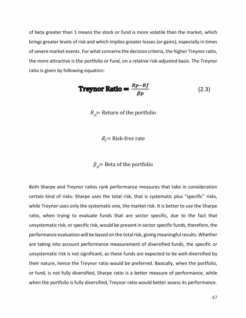
Treynor Ratio ................................................................................................. 46

Jensen's alpha ................................................................................................ 48

Modigliani-Modigliani Measure ............................................................................ 50

Sortino Ratio .................................................................................................. 51

Information Ratio ............................................................................................. 54

ALTERNATIVE PERFORMANCE MEASURES ............................................................ 55

Fama and French Three Factor Model .................................................................. 56

The Grinbblatt and Tiltman Model ........................................................................ 58

DATA ENVELOPMENT ANALYSIS (DEA)................................................................................. 60

INTRODUCTION TO DEA ..................................................................................... 60

4

LITERATURE REVIEW ......................................................................................... 63

DEA BASIC MODELS .......................................................................................... 68

CCR Model .................................................................................................... 68

BCC Model .................................................................................................... 76

Additive Model ................................................................................................ 80

DEA MODELS FOR INVESTMENT FUNDS VALUATION ............................................... 83

MURTHI, CHOI and DESAI Model ....................................................................... 84

BASSO and FUNARI Model ............................................................................... 87

MOREY and MOREYI Model .............................................................................. 90

GREGORIU, SEDZRO and ZHU Model ................................................................ 93

EMPIRICAL APPLICATION OF DEA APPROACH: EVALUATION OF ITALIAN FUNDS ............... 97

Introduction .................................................................................................... 97

Data Sample and Methodology ........................................................................... 98

Results ........................................................................................................ 103

CONCLUSION ....................................................................................................................... 117

BIBLIOGRAPHY .................................................................................................................... 119

SITOGRAPHY ....................................................................................................................... 122

5

Introduction

How can a non-institutional investor choose, rationally, in which investment fund put his

savings? Is the expected return enough to assess the performance of a fund? Do

traditional risk-adjusted measures give an overall judgement about funds’ efficiency?

This thesis aims to provide satisfying answers to questions like these, trying to present

the theoretical pillars and tools to evaluate funds’ performance along with an empirical

analysis on investment funds’ efficiency.

Investment funds, especially in the last two decades, have seen an important growth,

conceived as the most used mean of investment for non-professional investors.

Usually, funds’ performances are quantified on the basis of returns, though overlooking

several variables that may affect the overall judgement.

Through Data Envelopment Analysis (DEA), that is a non-parametric approach applied in

many fields for measuring performance and efficiency, important inputs, such as funds’

fees, will be part of evaluation analyses, allowing to deploy as many inputs and outputs

as possible.

The First chapter will introduce the concept of investment fund, classifying it by structure,

investment objective, and management attitude. Furthermore, it will be illustrated, how

funds are regulated in the two largest worldwide markets, Europe and United States,

highlighting differences and similarities within the underlying regulatory bodies.

Moreover, the first chapter will deal with the description of most important fees and

commissions, to conclude with benefits and downsides.

The second chapter will treat the most well-known risk-adjusted performance measures,

among which there are the Sharpe ratio, Sortino and Jensen’s alpha.

6

In the third chapter it will be presented a detailed definition of the potentiality of the DEA

tool, beginning from the literature review, going through different kind of applications

within various fields, culminating with the presentation of generic and specific funds’

efficiency evaluation DEA models.

In the fourth and last chapter, there is the introduction of an empirical application of a

specific DEA model, Murthi, Choi and Desai, to a sample of Italian investment funds. The

objective of this analysis is to assess the weight of transaction costs on the overall

performance. More precisely it will be considered the Total Expense Ratio (TER) and load

commissions, comparing the results of the DEA model with traditional risk-adjusted

measure. To conclude, it is computed the correlation between DEA results and two of the

most used performance gauge, to assess the soundness of analysis’ results.

7

Investment Funds

Defining Investment Funds

An investment fund is a financial company that pools capital from many subjects and

invests it in stocks, bonds or other assets1. This is the definition provided by the Security

Exchange Commission, the governmental commission that regulates the financial market

in the U.S. Instead, for the European Central Bank, an investment fund is a collective

investment undertaking that invests capital raised from the public in financial and non-

financial assets2. Even though the definitions use a different nomenclature, the

underlying concept is the same. Funds invest the money they collect into securities and

other financial assets, combining them into portfolios, groups of stocks or bonds owned

by the fund. Each fund share stands for an investor’s proportionate ownership of the

fund’s portfolio.

There are several types of funds in the market, classified by the features that characterize

them. Basically, funds can be broadly divided into three main categories: Open-end funds

(generally known as mutual funds), Closed-end funds and Unit Investment Trusts (UITs).

Then, as it will be described later on, open-ended funds can be divided in many others

sub-categories, such as stock funds, fixed-income funds, ETFs, money market funds etc…

1 Definition of Investment Fund given by the Security Exchange Commission:

https://www.sec.gov/investor/tools/mfcc/mutual-fund-help.htm 2 This definition of investment fund is written in the Regulation ECB/2007/8 published in the Official Journal (OJ) of

the European Union on 11 August 2007, and entered into force on 31 August 2007. Link

:https://www.ecb.europa.eu/ecb/legal/pdf/l_21120070811en00080029.pdf

8

Funds’ shares are bought and sold, or redeemed, to investors directly, or through the

brokerage of a professional intermediary. When buying shares in mutual funds, individual

investors cannot make decisions about the composition of portfolios. They simply have

the possibility to choose in which fund invest their money, based on investors’ level of

risk aversion and on goals, by looking at the return they want to yield from the

investment. Who oversees and makes decisions concerning which stocks or bonds should

pick, in what quantities and the timing of decisions, is the fund, or portfolio, manager.

The graph below shows in three simple steps how an investment fund process works:

Figure 1.1: Investment Fund Scheme

Source: RBC Global Asset Management, http://funds.rbcgam.com

The relevance of mutual funds, as one of the most used mean of investment, especially

9

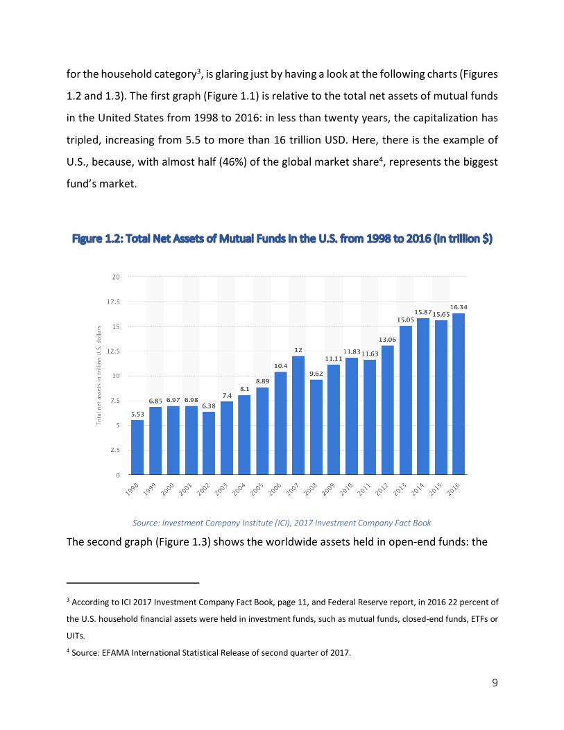
for the household category3, is glaring just by having a look at the following charts (Figures

1.2 and 1.3). The first graph (Figure 1.1) is relative to the total net assets of mutual funds

in the United States from 1998 to 2016: in less than twenty years, the capitalization has

tripled, increasing from 5.5 to more than 16 trillion USD. Here, there is the example of

U.S., because, with almost half (46%) of the global market share4, represents the biggest

fund’s market.

Figure 1.2: Total Net Assets of Mutual Funds in the U.S. from 1998 to 2016 (in trillion $)

Source: Investment Company Institute (ICI), 2017 Investment Company Fact Book

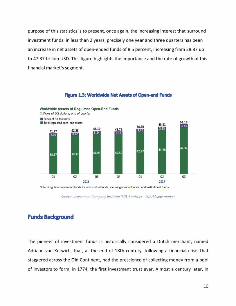
The second graph (Figure 1.3) shows the worldwide assets held in open-end funds: the

3 According to ICI 2017 Investment Company Fact Book, page 11, and Federal Reserve report, in 2016 22 percent of

the U.S. household financial assets were held in investment funds, such as mutual funds, closed-end funds, ETFs or

UITs. 4 Source: EFAMA International Statistical Release of second quarter of 2017.

10

purpose of this statistics is to present, once again, the increasing interest that surround

investment funds: in less than 2 years, precisely one year and three quarters has been

an increase in net assets of open-ended funds of 8.5 percent, increasing from 38.87 up

to 47.37 trillion USD. This figure highlights the importance and the rate of growth of this

financial market’s segment.

Figure 1.3: Worldwide Net Assets of Open-end Funds

Source: Investment Company Institute (ICI), Statistics – Worldwide market

Funds Background

The pioneer of investment funds is historically considered a Dutch merchant, named

Adriaan van Ketwich, that, at the end of 18th century, following a financial crisis that

staggered across the Old Continent, had the prescience of collecting money from a pool

of investors to form, in 1774, the first investment trust ever. Almost a century later, in

11

1868, with the scope of giving the possibility to invest money exploiting the benefits of

diversification, was established in London the “Foreign and Colonial Investment Trust”,

considered the first ever investment trust of the modern era. The first ever open-ended

mutual fund was created on March 21st, 1924, when three Boston securities executives

decided to pool their money to establish the “Massachusetts Investors Trust” (MIT), event

that would have revolutionized the financial industry and showing just from the beginning

unforeseen results: in the first year, the mutual fund grew from USD 50,000 to USD

329,000 in assets. American investors embraced this innovation and started to invest

heavily in it.

To instill investors with the necessary confidence, and in response to the financial crisis

of 1929 and the Great Depression, the U.S. Congress passed a series of laws with the aim

of regulating the entire financial industry, that was barely unregulated until that moment.

With the Securities Act of 1933, the Securities Exchange Act of 1934, and the Investment

Company Act of 1940, the Legislator established the foundation of the actual regulation

and set standards with which investment funds must comply.

Therefore, since the creation of the MIT in 1929, the fund industry has enjoyed the fastest

growth rate of the financial industry. In 1949, the totality of assets held by investment

funds amounted to USD 2 billion; this value soared to USD 6.3 trillion at the outset of

2003, and more than USD16 trillion in 2016 only in the U.S., making mutual funds

America’s largest financial investment vehicles.

Fund Scheme by Structure

12

As a common convention, investment funds are classified into three main categories:

Open-end funds (commonly named mutual funds), Close-end funds and UITs. In turn,

funds can be divided into several varieties such as, stock (or equity) funds, bond funds,

balanced-mixed funds, money market funds, ETFs etc… The possible ways through which

investors can yield profits from investing in mutual funds are listed as follow; the first is

dividend payment: when underlying stocks earn money in the form of dividend, the fund

successively will distribute dividend income to shareholders. Capital gain distribution is

another kind of return to investors: this capital gain occurs when the fund sells a stock

that has increased in price. At the end of each year, investment funds will distribute

capital gains, net to any capital losses, to shareholders. Third kind of investors’ return is

the increased market price, and this happen when the market value increases.

Open-End Funds

An Open-end mutual fund is “an investment company registered with the U.S. Security

Exchange Commission (SEC) that issue shares of its stock to investors, invests in in an

investment portfolio on the shareholders’ behalf, and stands ready to redeem its shares

for an amount based on its current share price”5. This is the most common type of

collective investment scheme, unlike closed-end funds, investors buy shares directly from

the fund itself at their Net Asset Value (NAV6), or share price. The share price of mutual

fund, and traditional UITs, based on their NAV, is obtained dividing the NAV by the total

5 W. Ruppel, Wiley GAAP for Governments 2017: Interpretation and Application of Generally Accepted Accounting

Principle for State and Local Governments, 2017, pp. 228-229 6 Definition given by the SEC: “Net Asset Value or NAV of an investment company is the company’s total assets minus

its total liabilities”. Furthermore, mutual funds and UITs “generally must calculate their NAV at least once every

business day”, while for a closed-end fund this is not required because its shares are not redeemable.

13

shares outstanding, plus fees that the fund charges at purchase or redemption,

respectively named sales load (or purchase fee) and deferred sales load (or redemption

fee).

Open-ended funds are available in most developed countries, but the terminology and

operating rules may vary. Some examples are: U.S. mutual funds, UK unit trusts and

OEICSs, European SICAVs etc.… The major U.S. open-end funds are: The Vanguard Group’s

S&P 500 (tot. assets of USD $391 billion), PIMCO Total Return (tot. assets USD $73 billion),

Fidelity Investment’s Magellan (tot. assets USD $17 billion). To conclude, statistics show

that more than half of the open-ended funds are based in the Americas (mostly in North

America, U.S. and Canada), with remaining 36% in Europe and 13% between Australia and

Asia7.

Closed-End Funds

Unlike open-ended funds, closed-end funds, shorten CEFs, do not continuously issue or

redeem shares. Initially, there a public offering of shares, offered to the public with the

intermediary work of licensed brokers. Up to this point the process is the same as for

open-end mutual funds. The difference underlies in the fact that “to obtain shares after

a public offering is completed, an investor must purchase shares from other investors in

the secondary market (one of the exchanges or the over-the-counter (OTC) market”8.

Unlike the open-end funds, the price per share is determined by the market and is usually

different from the underlying value or NAV per share.

7 Source: ICI Global, Statistics: Worldwide Mutual Fund Market

https://www.ici.org/research/stats/worldwide/ww_q3_17 8 S. Anderson, J. Born, O. Schnusenberg, Closed-end Funds, Exchange-Traded Funds and Hedge Funds: Origin,

Functions and Literature, 2009, pp-4-5.

14

Unit Investment Trust (UIT)

A unit investment trust (UIT) is a SEC registered investment company that offer an

unmanaged portfolio of securities, given that it is not a management company, as both

open-end and closed-end, and have no board of directors. Furthermore, UIT has a

predetermined date for termination that varies according to the investments held in its

fixed portfolio. When UITs are dissolved, proceeds from the securities are either paid to

investors or reinvested in another trust9. Thus, UIT’s securities will not be sold or new

ones bought, except in certain limited situations such as bankruptcy of a holding.10

These trusts are built by a sponsor and marketed through brokers. An UIT portfolio may

hold one of several different types of securities. The two main types are equity

and bond trusts. Equity trusts are generally intended to provide capital appreciation and

dividend income, at the end of the period, corresponding to the termination date, the

trust liquidates and distributes the net asset value as earning to the unitholders.

Conversely, bond trusts, which can be related to corporate, government and national

bonds, pay periodic interests, often in relatively consistent amounts, until the first bond

in the trust matures. At this moment, the capitals from the redemption are distributed to

the clients as a kind of return of principal. The trust then continues paying the monthly

income amount until the next bond is redeemed. Bond trusts are intended for investors

seeking relative high level of income while carrying on low risks.

9 A guide to Unit Investment Trusts, Investment Company Institute,2007. 10 S. Anderson, J. Born, O. Schnusenberg, Closed-end Funds, Exchange-Traded Funds and Hedge Funds: Origin,

Functions and Literature, 2009, pp-5-6

15

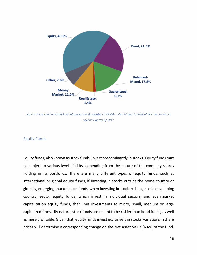
Fund Scheme by Investment Objective

All of the above-cited funds can be divided again into several sub-categories, based on

the securities’ nature of which they are composed of, such as equity, bond and balanced

funds. Moreover, there are Exchange Traded Funds and money market funds, which are

a specific type of mutual funds. There are also newer types of funds such as alternative,

smart-beta funds and esoteric ETFs, of which we’re not going to discuss. First of all, let’s

have a look at the global distribution of open-ended fund11 net assets at the end of the

second quarter of 2017 as presented by the following pie chart (Figure 1.4): more than

40% of these assets are invested in equity funds, followed by bond and balanced funds

respectively with 21.3% and 17.8%.

Figure 1.4: Worldwide Open-end Fund Net Assets by type of fund 2017, Q2

11 Here we have taken the open-end fund as a prototype of investment funds based on the fact that it is the most

widespread type of fund nowadays.

16

Source: European Fund and Asset Management Association (EFAMA), International Statistical Release: Trends in

Second Quarter of 2017

Equity Funds

Equity funds, also known as stock funds, invest predominantly in stocks. Equity funds may

be subject to various level of risks, depending from the nature of the company shares

holding in its portfolios. There are many different types of equity funds, such as

international or global equity funds, if investing in stocks outside the home country or

globally, emerging-market stock funds, when investing in stock exchanges of a developing

country, sector equity funds, which invest in individual sectors, and even market

capitalization equity funds, that limit investments to micro, small, medium or large

capitalized firms. By nature, stock funds are meant to be riskier than bond funds, as well

as more profitable. Given that, equity funds invest exclusively in stocks, variations in share

prices will determine a corresponding change on the Net Asset Value (NAV) of the fund.

17

Equity securities are by nature volatile and the factors that may influence their prices are

inflation, central bank policies, currency fluctuations, interest rates and so on and so

forth. However, an expert stocks fund’s manager will invest in varied companies, maybe

from different industries, generating diversification that reduces the volatility.

Fixed Income Funds

Fixed Income funds, also known as bond funds, invest primarily in bonds or other classes

of debt securities, and again it can be broken down into other subgroup, i.e. government,

municipal, corporate, convertible bonds and other debt securities. Due to the bond funds’

multiplicity, it is necessary to clarify that risks associated with bond funds may vary

consistently according to the subgroup of fund. These risks can be: credit, interest rate

and prepayment risks. For example, the credit risk is related to the chance of failure of

the company issuer of a specific bond: this will be less of a factor for funds investing in

government bonds (i.e. U.S. Treasury Bonds), given that the possibility of default of a

Nation is lesser than company’s one. Hence, funds investing in corporate bonds,

conceivably in firms with poor credit ratings, will face higher risk. Furthermore, the

interest rate risk is linked to the interest rate trend with funds investing in long-term

bonds having higher exposure to this kind of risk.

Balanced-Mixed Funds

18

A balanced fund, sometime called mixed or blended fund, may invest its assets in a wide

range of financial instruments, like money market accounts, bonds and equity, with the

intention to yield both growth in value and monthly income. This particular fund is geared

towards investors looking for a mix of capital appreciation and reduced riskiness, with

consistent level of diversification. Typically, stocks investment sums up between 50% and

70% of the balanced fund, with bonds accounting for the remaining, but there can be

further instruments in portfolios. However, every fund manager allocates weights in

different ways, and there is no set definition of how much of each a balanced fund should

or must contain.

Exchange Traded Funds (ETF)

Exchange Traded Funds (ETFs) are investment companies registered under the

Investment Company Act of 1940, in the U.S., as either open-ended funds or UITs, while

under the Undertaking for Collective Investment in Transferable Securities (UCITS)

Directive 2009/65/EC, in the European Union. Commonly known as index funds, ETFs are

intended to replicate the performance of their benchmark indexes, such as the NASDAQ-

100 Index, S&P 500, Dow Jones, etc... Contrary to conventional mutual funds, however,

ETFs are listed on an exchange and can be traded intra-daily. When an investor buys

shares of an ETF, he is buying shares of a portfolio that tracks the yield and return of a

broader index. The main difference between ETFs and other types of index funds is that

ETFs don't try to outperform their corresponding index, but simply replicate its

performance.

ETFs combines the benefits of both open-end and closed-end funds, combining the issuing

and redemption process of the former with the continuous stock market tradability of the

19

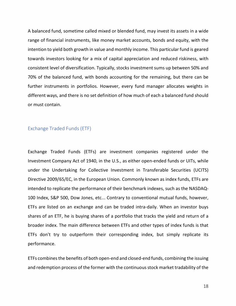
latter. ETFs have been around since the early 1980s, but they've come into their own

within last decade. As can be denoted from the graph below (Figure 1.5), across the period

2006-2016 the total ETFs’ assets increased from less than USD 600 billion to almost USD

3.5 trillion; this statistic discloses the enormous success that this particular investment

mean is having nowadays.

Figure 1.5: Assets’ development of global ETFs from 2003 to 2016

Source: Bloomberg; Deutsche Bank; Thomson Reuters (https://www.statista.com/statistics/224579/worldwide-etf-

assets-under-management-since-1997/)

20

Money Market Funds

Money market fund is a mutual fund that, by law, can invest only in high quality and short-

term securities, such as commercial paper, bankers’ acceptances, government bills and

repurchase agreement, paying dividends that generally replicate short-term interest

rates12. One of the main characteristic of money market funds is the constant value

around one dollar, not below, of Net Asset Value per share.

Money market funds’ category includes ones that invest primarily in government

securities, corporate and bank debt securities and tax-exempt municipal securities.

Moreover, these particular funds are usually intended for different types of investors such

as retail or institutional investors, when funds require high minimum investments.13 Many

investors use this type of funds to store cash or as an alternative to investing in the stock

market, also thanks to high liquidity and low riskiness of this instrument. The only risk

generally associated with money market funds is inflation risk, that may consume the

returns over time.

Money market funds are regulated primarily under the Investment Company Act of 1940

and the rules adopted under that Act, particularly Rule 2a-7 under the Act. Such funds are

not federally insured, although the portfolio may consist of guaranteed securities and/or

the fund may have private insurance protection.

12 A. Corrigan, P.C. Kaufman, Understanding Money Market Funds, 1987. 13 U.S. Security and Exchange Commission, Mutual Funds and ETFs, A Guide to Investors:

https://www.sec.gov/investor/pubs/sec-guide-to-mutual-funds.pdf

21

Fund Management: Active vs. Passive

Investment funds, regardless of whether they are actively or passively managed, share

common traits, that consist in three benefits to investors: diversification, straightforward

access to global securities markets and, above all, professional service of fund managers.

Basically, this is where the homogeneity between the two categories of managed

investment funds ends14. Active managed funds aim to beat the return from a particular

benchmark or market index, seeking to profit from identifying undervalued securities and

managing the weights of portfolios, in accordance with the knowledge and skills to

analyze and read into the market of funds’ managers. Active management can be

characterized by different investing styles: value and growth management. Value

management looks for firms whose shares are undervalued compared to their NAV, or

where managers see underestimated potential profits in the future. Instead, growth

management seeks for companies’ shares with above-average growth capacity over the

long-term.

In contrast, passive management, also known as index fund, attempts to track the

composition of an existent benchmark portfolio, based on the market efficiency

assumption. In order to match the benchmark, there are two different ways to operate:

from one side, buying all the stocks, maintaining the same proportions, appearing on the

benchmark index, while on the other side, and this is the more realistic case, identifying

14 Z. Bodie, A. Kane, A.J. Marcus, Investments and Portfolio Management: Global Edition, 2011, McGraw-Hill, 9th

Edition.

22

a bunch of stocks that can replicate accurately the benchmark’s performance. It is clear

that index fund’s management is much easier than active one, together with lower costs

for the investor, and consequently lower margins for the management. These are the

reasons why the supply of index funds in the market is scarce: one example of passive

management funds is represented by ETFs (Exchange Traded Funds), that have the

peculiarity of being traded exclusively in stock exchanges.

Regulation

In this paragraph, there will be presented some of the most relevant aspects concerning

investment funds’ regulation in U.S. and European Union. By highlighting the guidelines

and legislative cornerstones from which the regulatory frameworks take shape (i.e. the

Securities Act of 1933 and Securities Exchange Act of 1934 or the UCITS Directive

2014/91/EU) will be depicted the rationales and objectives underlying mutual funds’

regulatory background.

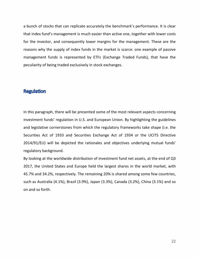
By looking at the worldwide distribution of investment fund net assets, at the end of Q3

2017, the United States and Europe held the largest shares in the world market, with

45.7% and 34.2%, respectively. The remaining 20% is shared among some few countries,

such as Australia (4.1%), Brazil (3.9%), Japan (3.3%), Canada (3.2%), China (3.1%) and so

on and so forth.

23

Figure 1.6: Worldwide Distribution of Investment Funds Net Assets at the end of Q2 2017

Source: European Fund and Asset Management Association, International Statistical Release: Trends in Second

Quarter of 2017

Therefore, the majority of worldwide investment funds, are distributed amid U.S. and E.U.

This is why, we will treat the legislative frameworks underlying these 2 investment fund

markets, showing also the most relevant regulatory differences and similarities.

U.S. Regulatory Framework

As already explained, United States represents the biggest market for investment funds,

based on funds’ net assets. In addition, it is the birthplace of the first regulation on the

subject. Indeed, the Securities Act of 1933, along with Securities Exchange Act of 1934,

Investment Company Act of 1940, Investment Advisers Act of 1940 and extensive rules

issued by the Securities and Exchange Commission (SEC), constitute the primary source

24

of applicable law, forming the spinal column of United States financial regulation. These

laws were approved in response to the Wall Street crash of 1929 and the following Great

Depression, in order to regulate, in the interest of the public, the securities industry,

included the investment companies, that were basically unregulated until that moment.

Let’s have a quick look at the main regulatory sources cited above, starting from the oldest

one: The Securities Act of 1933. Also known as the “truth in securities” law, this rule was

conceived with two basic purposes: requiring that investors receive financial and other

significant information concerning securities being offered for public sale and prohibit

deception, misrepresentations, and other fraud in the securities’ sale15. In order to

accomplish these goals, one of the most relevant issue of the law is the information’s

disclosure through the registration process. With this kind of knowledge, investors may

make informed judgement about whether to purchase a company’s securities or not.

That’s why the Security Exchange Commission (SEC)16 requires this kind of information to

be accurate, even though could not guarantee it.

Therefore, the registration process requires information about company’s properties and

businesses, descriptions about securities to be issued, information about company’s

management and financial statements complying with accounting requirements. All these

information, enclosed in the registration statement and prospectus, become public, so

anyone can freely have access and make informed decision about purchasing of

securities, avoiding misleading advertisement issues17.

15 For additional information visit the Security Exchange Commission website at this link:

https://www.sec.gov/answers/about-lawsshtml.html#secact1933 16 The Securities Exchange Commission is the governmental agency established in 1934 responsible for the

enforcement of U.S. federal securities law and for the regulation of the commerce in stocks, bonds, and other

securities. 17 Section 17(a)(2) of the Securities Act of 1933 prohibits, in the offer or sale of any security by communication in

interstate commerce, “obtain[ing] money or property by mean of any untrue statement of a material fact or any

25

With the Security Exchange Act of 1934, was established the SEC. The Act empowers the

SEC with the required authority over all the aspect of the securities industry, including the

power to register, regulate and supervise all Wall Street’s operators. Among these

operators, there are also the entities known as stocks exchanges, such as the New York

Stock Exchange (NYSE), NASDAQ Stock Market, and the Chicago Board of Options,

commonly known also as Self-Regulatory Organizations (SROs)18.

The Securities Exchange Act identifies and forbids certain classes of actions and provides

the Commission with disciplinary powers over regulated entities. More specifically, the

Act broadly prohibits fraudulent activities of any kind concerning the offer, purchase or

sale of securities. One of these is represented by the fraudulent insider trading19: this

conduct becomes illegal when someone trades securities while in possession of nonpublic

information, in violation of a duty to avoid trading. In addition, The Securities Exchange

Act also empowers the Commission to require periodic reporting of information by

companies with publicly traded securities.

For what concerns the Investment Company Act of 1940, it addresses the regulation of

companies, including investment funds, that are involved primarily in investing and

trading securities. Through this Act, the aim of the regulator was to minimize conflicts of

interests that could arise in these operations, by requiring the companies to disclose

information about fund’s structure, investment policies, and its operations. Again, the law

does not allow the SEC to directly oversee the investment activities of those companies.

The laws above described constitute the main body of the regulation in the U.S., but there

are other rules issued successively, like the Internal Revenue Code of

omission to state a material fact necessary in order to make the statements made, in light of the circumstances

under which they were made, not misleading.” 18 Section 7 (2)(b) of the Securities Exchange Act of 1934 19 Section 16(b) and indirectly through Section 10(b) of Securities Exchange Act of 1934

26

1986 (IRC) through which the regulator imposes requirements on funds willing to exploit

the favorable tax treatment afforded to regulated investment companies20.

E.U. Regulatory Framework

The European Union with EUR 14.8 trillion investment fund assets, at the end of Q3 of

2017, represents the second largest market with 34.2% of the worldwide assets invested

in funds. For this reason, it will be explained the regulatory framework underlying the E.U.

market of investment funds. Among these EUR 14.8 trillion, 8.6 trillion, almost 65% of all

funds’ assets in Europe, at the end of 2016, were held by 31,000 Undertakings for

Collective Investments in Transferable Securities (UCITS)21, Europe’s most important

collective investment scheme. While, an additional 27,000 Alternative Investment Funds

(AIF)22, of what the European Law refers to the non-UCITS collective investment scheme,

managed an overall EUR 5.5 trillion. Hence, UCITS and AIF are two of the most relevant

investment fund scheme used throughout the European Union.

The basis for European investment law is the Undertakings for Collective Investment in

Transferable Securities (UCITS) Directive, adopted in 198523, aimed to offer business and

20 B. Chegwidden, J. Thomas, S. Davidoff, Investment Funds in United States: Regulatory Overview, Practical Law

Company, 2013. 21 A UCITS is an investment fund scheme regulated by the European Union and the European Securities and Markets

Authority (ESMA) through which investors may have access to high quality and safe investment products. 22 Regulated by the Alternative Investment Fund Managers Directive (2011/61/EU) (AIFM Directive or AIFMD), AIFs

are defined as: funds that are not regulated by the UCITS Directive at European level. These include hedge funds,

real estate, private equity and other classes of institutional funds. 23 The Directive concerning the Undertaking for Collective Investment in Transferable Securities was embodied in

the Directive 85/611/EEC of the European Economic Community on 20th December 1985, representing complete and

harmonized framework covering collective investment schemes, that can be sold to retail investors throughout the

27

investment opportunities for both asset managers and investors by integrating the EU

market for investment funds. Progressively, there have been a series of new proposal and

updates of the Directive, until the latest version, the UCITS V, has been approved by the

European Parliament as Directive 2014/91/EU, which went into force in March 2016.

The UCITS Directive sets out a harmonized regulatory framework for investment funds

that raise capital from the public and invest it in certain classes of assets, providing high

levels of investor protection and a basis for the cross-border sale of these funds. Basically,

UCITS funds can be registered in Europe and sold to investors worldwide using unified

regulatory and investor protection requirements24. These funds are perceived as reliable

and well-regulated investments, very popular among investors who want to invest amid

diversified funds spread out within the European Union.

Whereas, Alternative Investment Funds (AIFs) are meant to be all investment funds that

are not already covered by the UCITS Directive. Such kind of Alternative Funds are for

well-informed investors, like institutional, qualified and professional ones. This particular

type of fund is regulated by the Alternative Investment Fund Manager Directive (AIFMD),

with EU Directive 2011/61/EU, requiring all covered AIFMs to obtain authorization, and

disclose various information in order to be allowed to operate in the market. The AIFMD

was motivated as part of a regulatory effort undertaken by G20 nations following the

global financial crisis of 2008. This Directive was intended with two major objectives built

into it. First, AIFMD seeks to protect investors, increasing transparency by AIFMs and

assuring that supervisors’ entities, the European Securities and Market Agency (ESMA)25,

European Union using a passport mechanism. This type of investment scheme accounts for 75% of all investment

funds across the European Union. 24 http://eimf.eu/aif_ucits_seminar/ 25 Jonathan Boyd, ESMA clarifies final guidelines on reporting obligations under AIFMD, Investment Europe.

Retrieved 20 April 2015.

28

and the European Systemic Risk Board (ESRB) have the necessary information they need

to monitor financial systems in the EU territory26. Investors’ protection is obtained

through the introduction of stricter compliance around the information disclosure27,

including conflict of interest and independent assets’ valuation.

The second aim of the Directive is to get rid of some of the systemic risk that the funds

can pose to the EU economy. To obtain this goal, the AIFMD requires the remuneration

policies must be structured in a way that does not encourage excessive risk taking, and

that financial leverage have to be reported to the ESRB.

To conclude, both U.S. and European investment funds’ regulatory frameworks, especially

after the global financial crisis of 2008, aim to protect private investor’s interests,

persisting in fighting against fraudulent actions. One of the key concept underlying these

regulations is the stricter compliance concerning the disclosure of information, which

translates into a claim for transparency, coming from the regulatory bodies.

Fund Structure

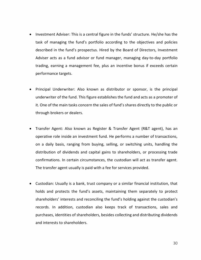
A classic example of mutual fund’s structure is given by the following scheme (Figure 1.7):

Figure 1.7: Structure of Investment Fund:

26 Niamh Moloney, EU Securities and Financial Markets Regulation, Oxford University Press. Retrieved 20 April 2015. 27 Articles 22 and 23 of the Directive 2011/61/EU (AIFMD)

29

Source: Investment Company Institute's (ICI) 2009 ICI Fact Book

where:

• Board of Directors: It serves the interests of shareholders, by managing the

company and handling the administrative issues. The Board of Directors is usually

elected by the board of shareholders. One of the task consists in suggesting a

preference of funds in order to meet the investment needs of shareholders. In

addition, the Board defines funds’ objectives and finally hires the investment

advisor, transfer agent and the custodian of the funds.

30

• Investment Adviser: This is a central figure in the funds’ structure. He/she has the

task of managing the fund’s portfolio according to the objectives and policies

described in the fund’s prospectus. Hired by the Board of Directors, Investment

Adviser acts as a fund advisor or fund manager, managing day-to-day portfolio

trading, earning a management fee, plus an incentive bonus if exceeds certain

performance targets.

• Principal Underwriter: Also known as distributor or sponsor, is the principal

underwriter of the fund. This figure establishes the fund and acts as a promoter of

it. One of the main tasks concern the sales of fund’s shares directly to the public or

through brokers or dealers.

• Transfer Agent: Also known as Register & Transfer Agent (R&T agent), has an

operative role inside an investment fund. He performs a number of transactions,

on a daily basis, ranging from buying, selling, or switching units, handling the

distribution of dividends and capital gains to shareholders, or processing trade

confirmations. In certain circumstances, the custodian will act as transfer agent.

The transfer agent usually is paid with a fee for services provided.

• Custodian: Usually is a bank, trust company or a similar financial institution, that

holds and protects the fund’s assets, maintaining them separately to protect

shareholders’ interests and reconciling the fund’s holding against the custodian’s

records. In addition, custodian also keeps track of transactions, sales and

purchases, identities of shareholders, besides collecting and distributing dividends

and interests to shareholders.

31

• Independent Public Accountant: Also known as Independent Auditor, this figure

performs an audit of fund’s financial statements and its records is filed with the

specific Commission (i.e. the SEC in the U.S.) in accordance with the securities law

or the Commission’s regulations28.

• Dealers: As mentioned before, the sponsor usually distributes shares of the mutual

fund through dealers or brokers. This figure is outside the legal boarders of the

investment fund but deserves to be quoted. Basically, the dealer purchases shares

from the sponsor at a discount and fill customers' orders.

Fund Fees and Expenses

As with any business, it costs money to invest in a fund. There are certain costs associated

with an investor’s transactions (such as buying, selling, or exchanging fund shares), which

are commonly known as “shareholder fees,” and ongoing fund operating costs (such as

investment advisory fees for managing the fund’s holdings, marketing and distribution

expenses, as well as custodial, transfer agency, legal, accounting, and other

administrative expenses). Even though these fees and expenses may not be listed

individually as specific line items on the account statement, they can have a substantial

impact on the investment return over time.

Fees and expenses differ among funds and the amount may depend on the fund

investment objective. Funds typically pay regular and recurring fund operating expenses

28 Robert A. Robertson, Fund Governance: Legal Duties of Investment Company Directors, 2001, Law Journal Press.

32

out of fund assets, instead of imposing these fees and charges directly on investors.

Because these expenses are paid out of fund assets, an investor will pay them indirectly.

Usually, these expenses are identified in the standardized fee table in the fund’s

prospectus under the heading “Annual Fund Operating Expenses”.

The fund’s directors, and its independent directors, in particular, function as “watchdogs”

who are supposed to look out for the interests of the fund’s shareholders. One of the

most significant responsibilities of a fund’s board of directors is to negotiate and review

the advisory contract between the fund and the investment adviser to the fund, including

fees and expense ratios.

For the reasons cited above, it is important for an individual, not professional, investor to

understand and be able to compare fees and expenses of different funds.

There are several classes of fees, as it will be described below, but for an investor to

facilitate the comparison between funds, it can be helpful to look at the Expense ratio29.

This is a percentage value expressing the annual fee that the funds or ETFs charge to

shareholders. Basically, it gives the percentage of assets deducted each fiscal year for

fund expenses, including 12b-130, management and administrative fees, operating costs,

and all other asset-based costs incurred by the fund, deducted from the fund's average

net assets, and accrued on a daily basis.

Fund transaction fees, or brokerage costs, as well as sales charges are not included in this

ratio. If the fund's assets are small, its expense ratio can be quite high due to the fact that

29 The expense ratio is the percentage of fund assets paid for operating expenses and management fees. It typically

includes the following types of fees: accounting, administrative, advisor, auditor, board of directors, custodial,

distribution (12b-1), legal, organizational, professional, registration, shareholder reporting, and transfer agency. The

expense ratio does not reflect the fund's brokerage costs or any investor sales charges. 30 Rule 12b-1, established with the Investment Company Act of 1940, allows mutual fund advisers to make payments

from fund assets for the costs of marketing and distribution of fund shares. The original rationale underlying the

plans was that such fees help attracting new shareholders into funds through marketing and advertisement and

providing incentives for brokers.

33

the fund must meet its expenses from a restricted asset base.

Conversely, as the net assets of the fund grow, the expense percentage should ideally

decrease as expenses are spread across the wider base.

Thus, the fees that an investor may pay when investing in mutual funds are the following:

• Transaction fee (Purchase fee): typically, is about purchase costs, it is charged

when the shareholder buys shares, and is paid to the fund, not to the stockbroker.

• Redemption fee (Exchange fee): another type of fee that funds charge their

shareholders when they sell or redeem shares, or exchange to another fund. Like

transaction fee, is paid to the fund too.

• Periodic fees: (which are included in the Expense Ratio)

- Management fee: paid, out of the fund assets, to the fund’s investment advisor

for portfolio management. Also called maintenance fees.

- Account fee: fees that fund separately impose in connection with the

maintenance of their account.

- Distribution and Service fee (12b-1 fee31): paid, out of the fund, to cover

marketing costs, cost of selling fund shares, and costs of providing shareholder

services. Is included in fund’s Expense ratio, generally between 0.25 and 1%

(the maximum allowed) of a fund’s net asset. 12b-1 fee can be broken down

into two distinctive charges: the distribution and marketing fee (maximum

0.75% annually) and the service fee (maximum 0.25% annually).

31 Named after section 12 of the Investment Company Act of 1940, https://www.sec.gov/about/laws/ica40.pdf

34

Benefits and Disadvantages of Investing in Funds

Benefits:

• Professional management: investment funds employing skilled and experienced

professionals, offer qualified investment services to investors. Fund management

analyses in detail past and present performance, financial statements and a series

of multiples and ratios of hundreds of companies selecting the best ones in order

to achieve the objective of the fund and ultimately satisfying shareholders.

• Diversification: Since one of the fundamental investment rule is the importance of

diversification, an investment fund can be a successful and easy way to achieve

this objective. The portfolio diversification allows to increase the expected return

meanwhile minimizing the risks. Therefore, investing in funds results in a cost-

effective way to reach this primary and basic goal for every investor.

• Liquidity: Investment funds, in particular Money Market Funds, have a significant

characteristic: the assets underlying these funds are generally liquid.

• Easy of comparison: For an average not professional investor, investment funds

are convenient also due to the ease of comparison between similar funds.

Investors can compare the funds based on metrics such as level of risk, return and

price, and given that this information are easily accessible, eventually everyone

may be able to make wise decisions, based on valid judgements.

35

• Potential return: Funds have the potential to provide high returns, depending on

the class of fund that is taken into consideration, to an investor than other options

over a reasonable period of time.

• Transparency: Thanks to the above described regulation, investment funds have

to disclose a detailed list of useful information allowing the average investor to

know as much information as possible about the companies where he or she is

going to invest money.

Disadvantages:

• Costs: Usually, investment funds have different fees that impact on the overall

payout. These fees can be shareholder or operating fees. The shareholder fees are

paid directly when purchasing or selling shares. Conversely operating fees are

charged as an annual percentage - usually ranging from 1 to 3%, and assessed to

fund investors regardless of the performance of the fund. Whether a fund is not

performing positively, these fees will have a negative impact on shareholders

returns, probably turning these one into losses.

• Misleading advertisement: The misleading advertisements of investment funds,

even if is prohibited by the general antifraud provision of federal securities law,

may conduct investors down the wrong path. In spite of the regulation on this

matter is quiet common bumping into misleading information concerning false

funds’ performance. It can happen that some funds are incorrectly labeled as

growth funds, while others are classified as small-cap or income.

36

• Fluctuating returns: Like the majority of investment means available in financial

markets, investment funds have not guaranteed returns. The price or Net asset

value of funds are volatile, except few cases of funds with stable values, so it can

appreciate or depreciate based on the expectations of the market and actors

playing in it. Unlike fixed-income products, such as bonds and Treasury bills, funds

experience price fluctuations along with the stocks that make up the fund. Another

important thing to be aware of is that investment funds are not guaranteed by any

national government, so in the case of dismissal, investors will not get any sort of

refund back.

37

Performance Measurement Methods of

Investment Funds

Performance Measures and Asset Pricing Models: An Overview

Before starting to describe and analyze some of the most important performance

valuation measures, it is useful to provide, as a theoretical background, an overview

regarding some asset pricing theories, models linking the portfolio’s expected returns

with volatility and other variables.

Once introduced these fundamental theories, the chapter will treat the description of

important performance metrics, which can be divided in two broad categories, risk-

adjusted and conventional methods. As it will be discussed below, asset pricing models

and performance measures are inseparably linked, and the evolution of the latter in the

literature mirrors the development of asset pricing models. A brief overview of this

parallel development should be useful.

Historically speaking, the origin of investment studies began with Markowitz’s

cornerstone on portfolio selection, from which all the subsequent theories and models

has taken form and got inspiration.

38

In 1952, Markowitz laid the foundation of “Modern Portfolio Theory”32, with his mean-

variance model. In its simplest form, Markowitz’s theory is about finding the optimal

balance between returns’ maximization and risks’ minimization. The objective of

Markowitz’s work was to select investments in such a way as to diversify risks while not

reducing the expected return. This represents one of the most important and influential

economic theories dealing with finance and investment.

Also known as “Portfolio Theory”, the model suggests that is possible to build an efficient

frontier of portfolios, giving the highest expected return for a given level of risk33. It is

actually simple to apply and effective. While it does not replace the role of an informed

investor, it can provide a powerful tool to complement an actively managed portfolio. The

theory suggests that by investing in more than one security, an investor can exploit the

benefit of diversification, which also translates in a riskiness’ reduction of portfolio. Keep

in mind that the risk of a portfolio composed by several individual stocks will be lower

than the risk intrinsic in holding any of the individual stocks alone.

The “Modern Portfolio Theory” assumes investors are risk averse and, when selecting

among portfolios, they care about mean and variance of the investment’s return. To

conclude, the resulting portfolio minimizes the variance of its return, given the expected

return, conversely maximizing the expected return, given the variance. For this reason,

Markowtiz’s theory is often considered a “mean-variance model”.

In other words, Markowitz, with his well-known theory, showed that investment is not

just picking stocks, but is about choosing the right combination of stocks among which

distributing the wealth.

32 H. M. Markowitz, Foundation of Portfolio Theory, Journal of Finance, Volume 46, Issue 2 (Jun, 1991), 469-477 33 H.M. Markowitz, Portfolio Selection. Journal of Finance, 7, 77-91, (1952).

39

Later, building on the work of Markowitz, Jack Treynor (1961-1962), William Sharpe

(1964), John Lintner (1965), Jan Mossin (1966), proposed a capital asset pricing model

(CAPM, 1964)34, a model that five decades later is still widely used, due to its simplicity

and utility, in several applications, such as firms’ cost of capital estimation and evaluating

the performance of managed portfolios.

Basically, the CAPM, demonstrates that, under certain conditions, the expected return of

an asset is only determined by the beta (b), also known as systematic risk or market risk.

This model is still used to determine a theoretically appropriate required rate of return

on an asset, in order to make decisions about assets’ composition in a well-diversified

portfolio.

The CAPM is based upon its assumptions, such as the efficiency and competitiveness of

the stocks’ market35, the presence in the market of rational and risk-averse investors,

market’s frictionless, that means there’s no transaction costs36, taxes, and restriction on

selling or short-selling. The model also requires limiting assumptions concerning the

statistical nature of securities returns and investors’ preferences. Finally, investors are

assumed to agree on the likely performance and risk of securities, based on the common

time horizon.

Although CAPM’s assumptions are unrealistic, such simplification of reality is often

necessary to develop trackable models. The true test of a model lies not just in the

34 E. F. Fama, K. R. French, The Capital Asset Pricing Model: Theory and Evidence, Journal of Economic Perspectives,

Volume 18, Number 3--Pages 25-46 35 This assumption presumes a financial market populated by highly-sophisticated and well-informed buyers and

sellers. 36 As it will be explained further on, transaction costs may influence the performance evaluation of investment funds,

hence this assumption is very strong, besides unrealistic.

40

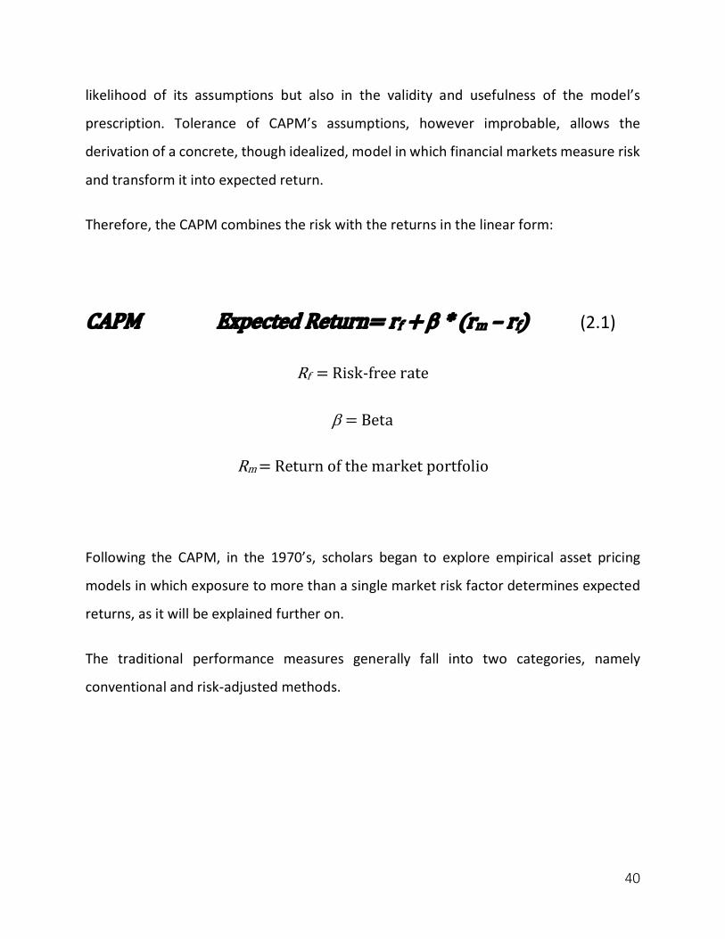
likelihood of its assumptions but also in the validity and usefulness of the model’s

prescription. Tolerance of CAPM’s assumptions, however improbable, allows the

derivation of a concrete, though idealized, model in which financial markets measure risk

and transform it into expected return.

Therefore, the CAPM combines the risk with the returns in the linear form:

CAPMExpectedReturn=rf+b*(rm–rf)(2.1)

Rf=Risk-freerate

b=Beta

Rm=Returnofthemarketportfolio

Following the CAPM, in the 1970’s, scholars began to explore empirical asset pricing

models in which exposure to more than a single market risk factor determines expected

returns, as it will be explained further on.

The traditional performance measures generally fall into two categories, namely

conventional and risk-adjusted methods.

41

Conventional Methods

Benchmark Comparison

Conventional methods most widely concern comparisons of the performance of

investment portfolio against broader market index. An example of benchmark market

index can be the U.S. Standard & Poor’s 500 index (S&P 500), which includes 500 stocks

issued by 500 large companies in the U.S.37. The S&P 50038 is widely considered the

leading indicator of U.S. securities, as well as the most accurate gauge of the performance

of large-cap American equities. However, it’s inappropriate compare a fund investing in

small-cap securities, or mainly in bonds, using the S&P 500 index as benchmark. For

example, the Barclays Capital U.S. Aggregate Bond Index39 is considered the benchmark

index for the bond market, while the Russell 2000 Index is suitable if considering small-

cap securities market, the MSCI EAFE Index for what concerns International stocks

(Europe, Australia and Far East), and to conclude the EURO STOXX Index if we need a

benchmark based on European stocks only. Hence, the right choice when considering

37 http://us.spindices.com/indices/equity/sp-500 38 This index is regarded as the best single gauge of large-cap U.S. equities. There is over USD 7.8 trillion benchmarked

to the index, with index assets comprising approximately USD 2.2 trillion of this total. The index includes 500 leading

companies and captures approximately 80% coverage of available market capitalization. 39 Also known as Bloomber Barclays U.S. Aggregate Bond Index, after 2016, is a broad-based benchmark that

measures the investment grade, U.S. dollar-denominated, fixed-rate taxable bond market, including Treasuries,

government-related and corporate securities, mortgage-backed securities, asset-backed securities and collateralized

mortgage-backed securities.

42

comparison method depends fundamentally on the specific market segment of

benchmark index, that clearly must mirror as much as possible the selection of securities

held by investor’s portfolio or directly by the mutual fund.

The Benchmark comparison method is quite simple: if the return on the portfolio exceeds

the one of the benchmark index, during the same time periods, then the portfolio is over-

performing the benchmark index, or simply have beaten the benchmark. Although this

type of comparison is very common in the investment world, this creates a particular

problem of evaluation. The level of risk of the investment portfolio may not be the same

as that of the benchmark index portfolio. Higher risk should lead to commensurately

higher returns, in the long-term. This means if the investment portfolio has performed

better than the benchmark portfolio it may be due to lower level of riskiness of the

investment portfolio compared to the benchmark. Therefore, a simple comparison of

returns, usually, may not produce consistent results, even if is widely used by common

“uninformed’ investors.

Style Comparison

A second conventional method of performance evaluation called ‘style-comparison’

involves comparison of return of portfolios having a similar investment style. While there

are many investment styles, one commonly used approach classifies investment styles as

value versus growth. The “value style” portfolios invest in companies that are considered

undervalued on the basis of criteria such as price-to-earnings (PE) and price-to-book (PB)

value multiples. The “growth style” portfolios invest in companies whose revenue and

earnings are expected to grow faster than those of the other companies. In order to

evaluate the performance of a value-oriented portfolio, it should be compared the return

43

on such a portfolio with that of a benchmark portfolio that is value style based. Similarly,

a growth style portfolio is compared with a growth style benchmark index. Once again,

here there is the same weakness presented above, that is to say a lack of risk’s

comparison: this method suffers from the fact that, while the style of the two compared

portfolios may look similar, their risks will probably be different. Also, the benchmarks

chosen may not be truly comparable in terms of the style since there can be many

important ways in which two similar style-oriented funds vary.

Risk-Adjusted Performance Measures

Based on the asset pricing models described earlier, many scholars, throughout the years,

had put forward a series of investment performance evaluation methods, classified as

risk-adjusted measures. These methods make adjustments to returns in order to take

account of the differences in risk’s levels between the investment fund and the

benchmark portfolio. Even though these kind of performance measures are popular

among investors and widely used in practice, they have theoretical flaws. Following, there

will be explained the major ratios and indexes used in the evaluation of performance, and

outlined advantages and disadvantages tied to the application of these gauges. Although

the literature swarms with many such methods, the most well-known ratios are: Sharpe,

Treynor, Jensen alpha, Modigliani and Modigliani, Sortino and Information. These

measures along with their pros and cons are discussed below.

44

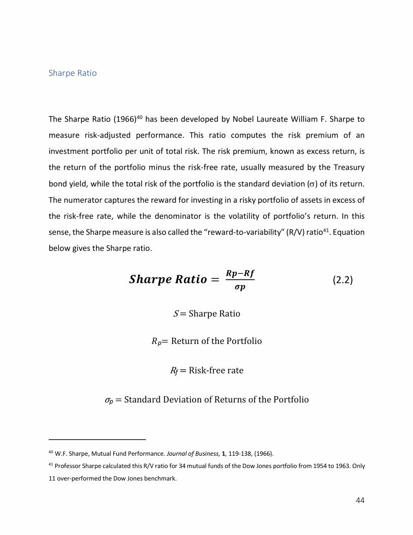
Sharpe Ratio

The Sharpe Ratio (1966)40 has been developed by Nobel Laureate William F. Sharpe to

measure risk-adjusted performance. This ratio computes the risk premium of an

investment portfolio per unit of total risk. The risk premium, known as excess return, is

the return of the portfolio minus the risk-free rate, usually measured by the Treasury

bond yield, while the total risk of the portfolio is the standard deviation (s) of its return.

The numerator captures the reward for investing in a risky portfolio of assets in excess of

the risk-free rate, while the denominator is the volatility of portfolio’s return. In this

sense, the Sharpe measure is also called the “reward-to-variability” (R/V) ratio41. Equation

below gives the Sharpe ratio.

𝑺𝒉𝒂𝒓𝒑𝒆𝑹𝒂𝒕𝒊𝒐 = 𝑹𝒑L𝑹𝒇𝝈𝒑

(2.2)

S=SharpeRatio

𝑅p= ReturnofthePortfolio

Rf=Risk-freerate

σp=StandardDeviationofReturnsofthePortfolio

40 W.F. Sharpe, Mutual Fund Performance. Journal of Business, 1, 119-138, (1966). 41 Professor Sharpe calculated this R/V ratio for 34 mutual funds of the Dow Jones portfolio from 1954 to 1963. Only

11 over-performed the Dow Jones benchmark.

45

Here, rp is the rate of return of a portfolio, rf is the risk-free rate, sp is the standard

deviation of fund’s return. Standard deviation is widely used to measure the degree of

fluctuation in a portfolio’s return. The larger the sp, the greater the magnitude of the

fluctuations from the portfolio’s average return. The Sharpe ratio is used to characterize

how well the return of an asset compensates the investor for the risk taken. This ratio is

very useful because although one portfolio or fund can reap higher returns than its peers,

it is only a good investment if those higher returns do not come with too much additional

risk. The greater a portfolio's Sharpe ratio, the better its risk-adjusted performance has

been. Investors are often advised to pick investments with high Sharpe ratios, because it

indicates that the investment has a higher risk premium for every unit of standard

deviation risk. However, like any mathematical model it relies on consistency of data.

When examining the investment performance of assets with smoothing returns the

Sharpe ratio should be derived from the performance of the underlying assets rather than

the fund returns.

Hence, the strengths of this ratio are its straightforwardness and simplicity as a

performance measure, using the standard deviation, including systematic and

unsystematic risk, which makes the Sharpe ratio suitable to evaluate portfolio and funds

returns that are not completely diversified, and also, with different trading strategies.

However, if on one hand standard deviation and expected returns are useful sources of

data in evaluation, on the other hand is really challenging to find the correct ones. As

always, in a highly stable environment, is possible to use past data, especially if

macroeconomics factors and competitive and market conditions haven’t changed much

in recent years. In a scenario like this, an estimate of returns and standard deviation over

46

the past period may be good predictors of what will happen in the future. Nevertheless,

in today’s dynamic markets, it is rare that the future replicates the past, hence the past

data are not reliable in order to make truthful appraisals. Again, standard deviation

includes movements in every direction, which may be considered a weakness because it

does not differentiate between upside and downside volatility.

Another Sharpe ratio’s weakness is its link with normal distributions. As a consequence,

the Sharpe ratio is not a suitable efficiency measure for investments with asymmetric, or,

generally, not Gaussian, expected returns. Last but not least, there is the fact that Sharpe

ratio provides a valuable information only when compared with a benchmark or another

investment, which leads to another challenging choice regarding the benchmark to be

used.

Treynor Ratio

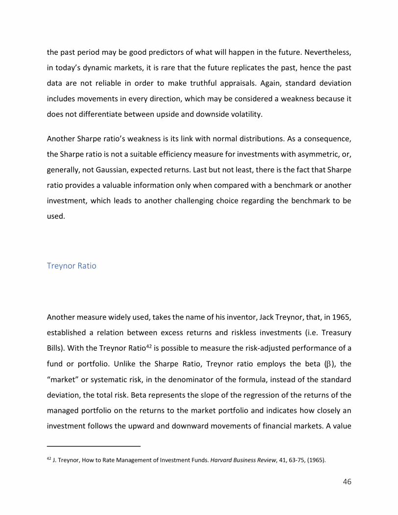
Another measure widely used, takes the name of his inventor, Jack Treynor, that, in 1965,

established a relation between excess returns and riskless investments (i.e. Treasury

Bills). With the Treynor Ratio42 is possible to measure the risk-adjusted performance of a

fund or portfolio. Unlike the Sharpe Ratio, Treynor ratio employs the beta (b), the

“market” or systematic risk, in the denominator of the formula, instead of the standard

deviation, the total risk. Beta represents the slope of the regression of the returns of the

managed portfolio on the returns to the market portfolio and indicates how closely an

investment follows the upward and downward movements of financial markets. A value

42 J. Treynor, How to Rate Management of Investment Funds. Harvard Business Review, 41, 63-75, (1965).

47

of beta greater than 1 means the stock or fund is more volatile than the market, which

brings greater levels of risk and which implies greater losses (or gains), especially in times

of severe market events. For what concerns the decision criteria, the higher Treynor ratio,

the more attractive is the portfolio or fund, on a relative risk-adjusted basis. The Treynor

ratio is given by following equation:

TreynorRatio= 𝑹𝒑L𝑹𝒇𝜷𝒑

(2.3)

𝑅p= Returnoftheportfolio

Rf=Risk-freerate

𝛽p= Betaoftheportfolio

Both Sharpe and Treynor ratios rank performance measures that take in consideration

certain kind of risks: Sharpe uses the total risk, that is systematic plus “specific” risks,

while Treynor uses only the systematic one, the market risk. It is better to use the Sharpe

ratio, when trying to evaluate funds that are sector specific, due to the fact that

unsystematic risk, or specific risk, would be present in sector specific funds, therefore, the

performance evaluation will be based on the total risk, giving meaningful results. Whether

are taking into account performance measurement of diversified funds, the specific or

unsystematic risk is not significant, as these funds are expected to be well-diversified by

their nature, hence the Treynor ratio would be preferred. Basically, when the portfolio,

or fund, is not fully diversified, Sharpe ratio is a better measure of performance, while

when the portfolio is fully diversified, Treynor ratio would better assess its performance.

48

The strengths of this ratio underlies mostly on the use of beta as a risk’s measure: first of

all because it distinguishes, again, between systematic and unsystematic risk; then

because beta is inherently more stable than standard deviation, as risk gauge. As well as

it has been done before, it will be described also the weaknesses, that are similar to the

Sharpe’s ones. The ratio assumes that the portfolio under evaluation is fully diversified,

given that only systematic risk is taken into account, measuring only market risk. Like the

Sharpe ratio, this is exclusively meant as a ranking criterion, and by the way is useful only

when are considering sub-portfolios of a broader, fully diversified portfolio; if this is not

the case, assets with the same systematic risk, but different total risk, will be ranked the

same. Another similarity with the previous measure is based on the backward-looking

nature. Investments will inevitably show different performances in the future than the

past ones.

Jensen’s alpha

Developed by American economist Michael Jensen in 1968, this model, based on the

Capital Asset Pricing Model (CAPM), is used to determine the abnormal return of a

security or portfolio over the theoretical expected return. In short, Jensen’s alpha43 tries

to explain whether an investment has performed better or worse than its beta value

would suggest. The alpha is simply the intercept from a regression of fund excess returns

on market excess returns. According to the CAPM the intercept alpha should be zero, so

the extent to which alpha differs from zero measures the extent to which the CAPM is

unable to account for the returns of the fund or asset. This means that alpha measures

43 M.C. Jensen, The Performance of Mutual Funds in the Period 1945-1964. Journal of Finance, 23, 389-416, (1968).

49

abnormal performance relative to a theoretical expected return, based on the capital

asset pricing model.

Hence, alpha can be greater than, less than or equal to zero. For example, an alpha greater

than zero suggests that the security outperformed its theoretical expected return.

Jensen’s alpha is given by equation below:

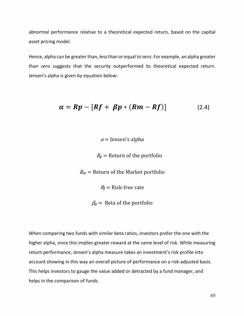
𝜶 = 𝑹𝒑 − [𝑹𝒇 + 𝜷𝒑 ∗ (𝑹𝒎− 𝑹𝒇)] (2.4)

α=Jensen'salpha

Rp=Returnoftheportfolio

Rm=ReturnoftheMarketportfolio

Rf=Risk-freerate

βp=Betaoftheportfolio

When comparing two funds with similar beta ratios, investors prefer the one with the

higher alpha, since this implies greater reward at the same level of risk. While measuring

return performance, Jensen’s alpha measure takes an investment’s risk profile into

account showing in this way an overall picture of performance on a risk-adjusted basis.

This helps investors to gauge the value added or detracted by a fund manager, and

helps in the comparison of funds.

50

A common weakness of both Jensen alpha and Treynor ratio is that both require an

estimate of beta, which can differ a lot depending on the source of data provider. This in

turn can lead to a mismeasurement of risk-adjusted return. Like the previous two

measures, even Jensen’s alpha is subject to generic weaknesses of the CAPM, and those

linked to the mean-variance world.

Modigliani-Modigliani Measure

Franco Modigliani and Leah Modigliani44 propose a modified version of Sharpe's

measurement approach. They shared the view that the Sharpe ratio was too difficult to

understand for the average investor, for this reason they proposed the “RAP” (Risk-

adjusted performance) ratio, also referred to as M2, or Modigliani-Modigliani Measure.

This measure expresses a fund’s performance relative to the market in percentage terms.

They believed that the average investor would find the measure more comprehensive.

Analytically their approach is the following:

RAP= 𝝈𝒎𝝈𝒑∗ (𝑹𝒑 − 𝑹𝒇) + 𝑹𝒇 (2.5)

Rp=Returnoftheportfolio

Rf=Risk-freerate

44 F. Modigliani, L. Modigliani, Risk-Adjusted Performance. Journal of Portfolio Management, 23, 45-54, (1997).

51

σm=Ex-postStandardDeviationofthemarket

σp=Ex-postStandardDeviationofportfolio

Modigliani and Modigliani propose to use the standard deviation of a broad market index,

i.e. the S&P 500, as the benchmark for comparison. In simple terms, for any fund with

certain return and level of risk, the M2 measure is equal to the return the fund would have

performed if it had the same risk as the market index. Therefore, the fund with the highest

“RAP”, or Modigliani, measure would have the highest return for any level of risk. The

peculiarity, compared with the Sharpe ratio, is that, since the Modigliani measure is

expressed in percentage points, it can be easily understood by average investors.

In opposite to Sharpe who used to rank funds according to the slope of the capital market

line, Modigliani and Modigliani lever or unlever, depending if the portfolio’s standard

deviation is higher or lower than the market one, portfolio’s risk to match market risk and

present the resulting risk-adjusted return as the ranking variable. This approach produces

the same ranking as obtained by applying the Sharpe Ratio, but in an easier way to be

understood. As it can be simply inferred, the Modigliani measure has the same limitations

as the Sharpe ratio.

Sortino Ratio

In the early 1980s, Frank Sortino, who was working for the Pension Research Institute,

had undertaken research to come up with an improved measure for returns. The Sortino

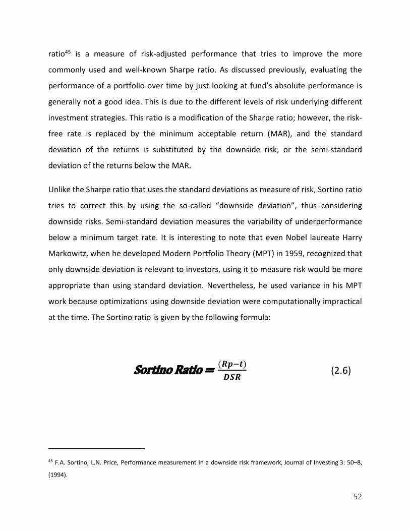
52

ratio45 is a measure of risk-adjusted performance that tries to improve the more

commonly used and well-known Sharpe ratio. As discussed previously, evaluating the

performance of a portfolio over time by just looking at fund’s absolute performance is

generally not a good idea. This is due to the different levels of risk underlying different

investment strategies. This ratio is a modification of the Sharpe ratio; however, the risk-

free rate is replaced by the minimum acceptable return (MAR), and the standard

deviation of the returns is substituted by the downside risk, or the semi-standard

deviation of the returns below the MAR.

Unlike the Sharpe ratio that uses the standard deviations as measure of risk, Sortino ratio

tries to correct this by using the so-called “downside deviation”, thus considering

downside risks. Semi-standard deviation measures the variability of underperformance

below a minimum target rate. It is interesting to note that even Nobel laureate Harry

Markowitz, when he developed Modern Portfolio Theory (MPT) in 1959, recognized that

only downside deviation is relevant to investors, using it to measure risk would be more

appropriate than using standard deviation. Nevertheless, he used variance in his MPT

work because optimizations using downside deviation were computationally impractical

at the time. The Sortino ratio is given by the following formula:

SortinoRatio= (𝑹𝒑L𝒕)𝑫𝑺𝑹

(2.6)

45 F.A. Sortino, L.N. Price, Performance measurement in a downside risk framework, Journal of Investing 3: 50–8,

(1994).

53

Rp=Returnoftheportfolio

t=MinimumAcceptableReturnorMAR

DSR=DownsideRisk

As mentioned above, this ratio adjusts the average return of portfolio with a target return

(MAR). The choice of the target or minimum acceptable return depends on the

investment goal of the fund, that is implicitly claimed through its strategy. The higher the

portfolio return over the MAR, the higher will be the Sortino ratio.

This ratio is intended to be compared, like the previous measures, with other comparable

funds or benchmark index. A higher Sortino ratio indicates better risk-adjusted

performance. In order to compare funds’ performance, the ratio of each fund must have

an equal MAR.

The interpretation of this ratio is less straightforward than the Sharpe ratio, due to the

fact that the measure of risk has a less direct interpretation than the standard deviation

and the choice of the target return (MAR) depends on the fund’s chosen strategy.

By the way, the Sortino ratio appears to overcome some of the issues underlying the

application of the Sharpe ratio: it combines a relevant return target in both numerator

and denominator of the formula; it assesses downside volatility without penalizing the

upside one, and as a consequence of this peculiarity, it is also more applicable to

distributions that are negatively skewed compared to other standard deviation based

measures. Moreover, drawing a parallel between the Sharpe and Sortino ratios for a fund,

it can be identified which portion of the volatility of the fund is related to outperformance

versus underperformance.

On the other hand, since this ratio only incorporates downside volatility below the

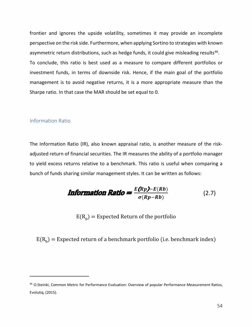
54

frontier and ignores the upside volatility, sometimes it may provide an incomplete

perspective on the risk side. Furthermore, when applying Sortino to strategies with known

asymmetric return distributions, such as hedge funds, it could give misleading results46.

To conclude, this ratio is best used as a measure to compare different portfolios or

investment funds, in terms of downside risk. Hence, if the main goal of the portfolio

management is to avoid negative returns, it is a more appropriate measure than the

Sharpe ratio. In that case the MAR should be set equal to 0.

Information Ratio

The Information Ratio (IR), also known appraisal ratio, is another measure of the risk-

adjusted return of financial securities. The IR measures the ability of a portfolio manager

to yield excess returns relative to a benchmark. This ratio is useful when comparing a

bunch of funds sharing similar management styles. It can be written as follows:

InformationRatio= 𝑬(𝑹𝒑)L𝑬(𝑹𝒃)𝝈(𝑹𝒑L𝑹𝒃)

(2.7)

E(Rp)=ExpectedReturnoftheportfolio

E(Rb)=Expectedreturnofabenchmarkportfolio(i.e.benchmarkindex)

46 O.Steinki, Common Metric for Performance Evaluation: Overview of popular Performance Measurement Ratios,

Evolutiq, (2015).

55

σ(Rp-Rb)=TrackingError(St.Dev.ofdifferencebetweenRp and Rb)

Since IR measures managers’ ability to generate higher returns relative to a benchmark

portfolio, from the formula it’s evident that, in order to generate value for shareholders

(investors), managers should maximize the expected active return (numerator) and

minimize the cost of their active management style (denominator). A higher IR suggests

that managers can achieve higher returns without taking on additional risks.

Alternative Performance Measures

All the measures described above, have their theoretical foundation on the CAPM model.

Many authors argue that the single market risk factor, Beta (b) in the CAPM, is not

sufficient to assess funds’ returns. For this reason, various factors, such as

macroeconomic, industry and firm related, have been proposed in the literature in order

to provide more reliable portfolio performance’s measures. Multi-factor pricing model

was an attempt to provide more reliability in this field. Multifactor pricing models were

presented by Ross (1976) through the Arbitrage Pricing Theory47 and by Merton (1973)

through the Intertemporal CAPM. The multifactor pricing model implies that the expected

return on an asset is a linear function of factor risk premiums and their associated factor

sensitivities. The underlying theory is, however, not very explicit on the exact nature of

47 S. Ross, The arbitrage theory of capital pricing, Journal of Economic Theor, (1976).

56

these factors. The selection of an appropriate set of factors is thus largely an empirical

issue.

Chen et al. (1986) find evidence of five priced macroeconomic factors. The Fama and

French study uses firm characteristics to outline factor portfolios resulting in the well-

known three-factor model, while Carhart (1997) finds evidence for a fourth momentum

factor. Other approaches rely on macroeconomic factors like interest and inflation rates.

Some include indexes that are related to managers’ investment style (e.g. small-growth

capitalization; large-value capitalization, etc...). Thus, there is a lack of consensus among

scholars about the number and the exact identity of the factors.

Fama and French Three-Factor Model

Some other scholars used multi-factor models based on the Arbitrage Pricing Theory

(APT), to evaluate the performance of mutual funds, of which the Three-Factor Model48

and four-factor model are the most representative. The Fama and French Three-Factor

model states that in an equilibrium market the arbitrage portfolio must be zero, meaning

that an arbitrage portfolio cannot exist. If this condition did not hold market participants

would sell assets whose expected return is lower than implied by the detected common

risk factors of the market and buy assets whose expected return is higher than implied by

the risk factors. This process of arbitrage ensures equilibrium as market participants

48 Fama Eugene F., French Kenneth R., "Common Risk Factors in the Returns on Stocks and Bonds", Journal of

Financial Economics, February, (1993).

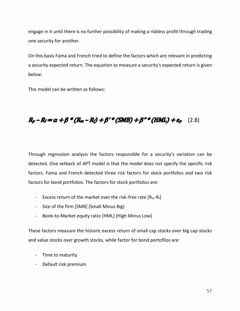
57

engage in it until there is no further possibility of making a riskless profit through trading

one security for another.

On this basis Fama and French tried to define the factors which are relevant in predicting

a security expected return. The equation to measure a security's expected return is given

below:

This model can be written as follows:

Rp–Rf=a+b*(Rm–Rf)+b’*(SMB)+b”*(HML)+ep(2.8)

Through regression analysis the factors responsible for a security's variation can be

detected. One setback of APT model is that the model does not specify the specific risk

factors. Fama and French detected three risk factors for stock portfolios and two risk

factors for bond portfolios. The factors for stock portfolios are:

- Excess return of the market over the risk-free rate [Rm-Rf]

- Size of the firm [SMB] (Small Minus Big)

- Book-to-Market equity ratio [HML] (High Minus Low)

These factors measure the historic excess return of small cap stocks over big cap stocks

and value stocks over growth stocks, while factor for bond portoflios are:

- Time to maturity

- Default risk premium

58

Fama and French propose their findings as being useful for portfolio performance

evaluation but did not pursue it per se.

The Grinbblatt & Titman Model

The problem concerning the choice of right benchmark have led to alternative approaches

to determine the performance of a portfolio or a fund. Grinbblatt and Titman49, pursued

an approach where no benchmark is needed, thus alleviating several problems tied to the

benchmark’s employment. The greatest issue and constraint of their model underlies in

the characteristics that is only applicable if the exact composition of portfolio or fund is

known. This is in strong contrast to the portfolio measures introduced earlier since they

allowed portfolio performance evaluation without apprehending its composition.

The underlying rationale of their model, named "Portfolio Change Measure" (PCM), is that

an informed investor, an investor who knows the exact composition of a portfolio, will

adjust his portfolio’s weights towards assets with higher expected returns and lower risks

than average as much as get rid of assets with expected returns lower than average. This

operation will generate a positive covariance between portfolio’s weights and the return

of a security for an informed investor, though it should not be any covariance between

portfolio’s weights and the return of an asset for the investor who is not informed.

Grinblatt and Titman propose to measure this covariance in the following way:

49 M. Grinblatt, S. Titman, Performance Measurement without benchmarks: An Examination of Mutual Fund Returns,

The Journal of Business, vol.66, issue 1, 47-68, (1993).

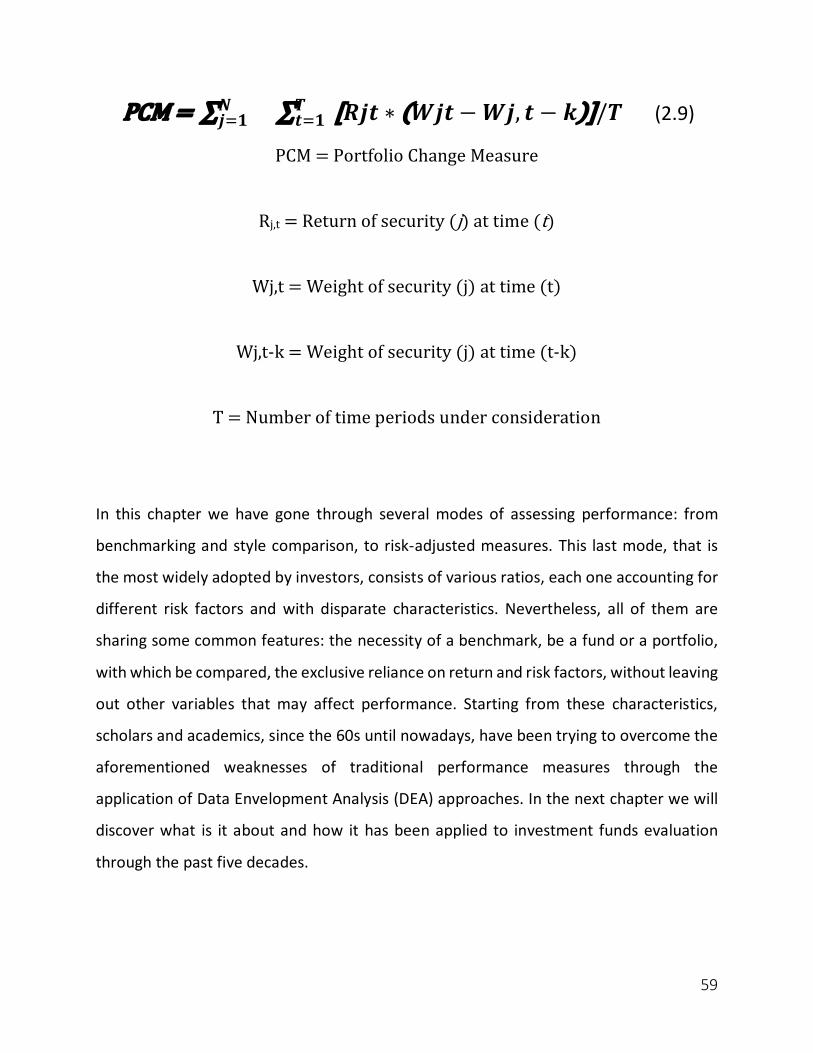
59

PCM=∑𝑵𝒋q𝟏 ∑ [𝑹𝒋𝒕 ∗ (𝑾𝒋𝒕 −𝑾𝒋, 𝒕 − 𝒌)]/𝑻𝑻𝒕q𝟏 (2.9)

PCM=PortfolioChangeMeasure

Rj,t=Returnofsecurity(j)attime(t)

Wj,t=Weightofsecurity(j)attime(t)

Wj,t-k=Weightofsecurity(j)attime(t-k)

T=Numberoftimeperiodsunderconsideration

In this chapter we have gone through several modes of assessing performance: from

benchmarking and style comparison, to risk-adjusted measures. This last mode, that is

the most widely adopted by investors, consists of various ratios, each one accounting for

different risk factors and with disparate characteristics. Nevertheless, all of them are

sharing some common features: the necessity of a benchmark, be a fund or a portfolio,

with which be compared, the exclusive reliance on return and risk factors, without leaving

out other variables that may affect performance. Starting from these characteristics,

scholars and academics, since the 60s until nowadays, have been trying to overcome the

aforementioned weaknesses of traditional performance measures through the

application of Data Envelopment Analysis (DEA) approaches. In the next chapter we will

discover what is it about and how it has been applied to investment funds evaluation

through the past five decades.

60

Data Envelopment Analysis (DEA)

Introduction

All the risk-adjusted performance measures introduced above are very popular among

investors and widely used in practice, though they all have in common theoretical flaws,

as it has been described in the previous chapter. In this chapter, we are going to introduce,

describe and analyze a different methodology used to measure efficiency and assess

performance: Data Envelopment Analysis (DEA). Contrary to other performance

measures, the DEA technique has the distinctive characteristic of incorporating many

factors, named inputs and outputs, in addition to the classic variables of risk and return,

in the measurement process, offering investors a powerful tool for ranking mutual funds

by self-appraisal and peer group valuation50.

How does DEA provide insights to investors? DEA approach helps benchmarking mutual

funds on a relative basis instead of absolute performance measurement as given by

traditional performance measures. Also, through this technique is possible to include the

50 H.R. Khedmatgozar, A. Kazemi, P. Hanafizadeh, Mutual Fund Performance Evaluation: a value efficiency analysis

approach, International Journal of Electronic Finance, (2013)

61

cost of owning a mutual fund share in the form of a fund’s expense ratio, load charges51,

12b-152 charges as an input variable in addition to fund’s objective, return and risk as

measured by beta and standard deviation of the fund.

The DEA methodology has many features that makes it a powerful tool in efficiency and

performance evaluation. One of these characteristics is also a unique advantage: DEA

doesn’t need the hypothesis of validity of the CAPM, eluding the effect of selection of

market portfolio and risk-free rate on the evaluation results. Another peculiar feature of

this approach concerns weights optimization: unlike other performance gauge techniques

like regression analysis, DEA don’t require to assign ex-ante particular weights to

parameters. This peculiarity is extremely important when, as it will be discussed sooner,

it comes to assess investment funds’ or portfolios performance. Another great feature of

DEA is that it doesn’t require uniformity of units of analysis regarding inputs and outputs.

DEA methodology was used for the first time in Germany to estimate the marginal

productivity of R&D and other factors of production, however it has a wide variety of

applications: from assessment of education system, health-care and hospital efficiency to

banking, finance, agriculture, transportation and logistics industries performance

evaluation53. The application of DEA to the assessment of the performance evaluation of

investment funds have become even more relevant in the last years, when an increasing

number of papers published on international journals and academic books were written

on its application to conventional mutual funds, hedge funds and ETFs. Anyway, if we

51 It is referred to the sales charge or commission an investor pays to an investment advisor, or broker, for his/her

time and expertise in selecting an appropriate fund for the investor, based on his/her preferences. The load is either

paid up front at the time of purchase (front-end load), or when the shares are sold (back-end load). 52 Definition on paragraph “Mutual fund fees and expenses” Chapter 1. 53 A. Emrouznejad, B.R. Parker, G. Tavares, Evaluation of research in efficiency and productivity: a survey and analysis

of the first 30 years of scholarly literature in DEA. Socio-Economic Planning Sciences, (2008).

62

have a look at the performance metrics applied in the financial business to valuate and

compare mutual funds based on historical prices and performances, we discover that

results obtained with traditional and conventional measures, precisely the ones

employed by financial industry practitioners, are different from performance scores

obtained with DEA models. This dissimilarity may be attributed mainly to two reasons:

first, because of the difficulty of providing a transparent interpretation of DEA indicators

easily understandable by financial professional; secondly, due to the sophisticated nature

of DEA models, especially if compared to most known traditional performance measures

such as, Sharpe, Sortino or Treynor ratios54.

Above we have cited the criticized theoretical flaws that follow through traditional risk-

adjusted efficiency measures, affirming the useful and original disposition of DEA

approach, that is capable of capturing and measuring performances considering

additional variables. Therefore, what are these factors that can be related to mutual

funds’ performance, that the traditional measures did not take into account? For

example, as it has been described in the first chapter, funds’ fees and commissions (for

simplicity we can consider the Expense ratio), dimensions (fund assets) are factors that

could be included in an accurate efficiency evaluation, and even classification, of

investment funds. What follows is a literature review of the early studies that contribute

to the development and implementation of the basic DEA models.

54 J. Zhu, Data Envelopment Analysis: A Handbook of Empirical Studies and Applications, 2016, Springer, pp. 229-

230.

63

Literature Review

Let’s start with a generic definition of the data envelopment analysis. DEA is a non-

parametric approach, i.e. inputs and outputs related to the transformation process do not

need to have the same units of measurement55, a mathematical programming tool, that

can be applied in performance measurement and efficiency analysis. Cooper, Seiford and

Zhu (2004) define DEA as ‘a relatively new “data orientated” approach for evaluating the

performance of a set of peer entities, called Decision Making Units (DMUs), which convert

multiple inputs into multiple outputs’56. DEA in its current form was first introduced in

1978 and has been recognized as an excellent methodology for performance evaluations.

As such, DEA has been used in evaluating the performance of many different types of

business units and activities in the succeeding years. The term DMU was used to allow for

the model’s application to a wide variety of activities, including governmental, not-for-

profit and business units.

More specifically, DEA has to be considered a non-parametric approach to productivity

analysis, especially efficiency analysis, of DMUs. Indeed, since the introduction of the first

DEA model, namely the CCR model, in 1978, it has been widely used in efficiency analysis

of many businesses and industry evaluation procedures. The most well-known DEA

models are: the CCR model (Charnes, Cooper and Rhodes, 1978), the BCC model (Banker,

Charnes and Cooper, 1984) and the Additive model (1985).

55 Y Zhao, K Triantis, P Murray-Tuite, P Edara, Performance measurement of a transportation network with a

downtown space reservation system: A network-DEA system, Transportation Research Part E: Logistics and

Transportation Review, (2011) 56 W.W. Cooper, L.M. Seiford, J. Zhu, Handbook on Data Envelopment Analysis, (2011). Springer, Boston.

64

Charnes, Cooper and Rhodes, with their work57 of 1978, aimed to elaborate and develop

the concepts published by Farrell, two decades earlier, in 1957. Farrell wanted to create

innovative models for measuring the productivity. The measures available at that time

were accurate but too restrictive, due to the fact they did not allow to combine multiple

inputs in order to get a total efficiency measure. To address this problem, Farrell worked

out a method that was applicable to any productive organization, extending the concept

of productivity towards the efficiency.

Essentially, productivity is based on the ratio between the quantities of output and input

used in the production process. While, the concept of efficiency encloses the comparison

between productivity and the DMUs. Farrell define overall productive efficiency as the

product between technical and allocative efficiency58. Technical efficiency is measured as

the ratio between the observed output and the maximum output, under the assumption

of fixed input, or, alternatively, as the ratio between the observed input and the minimum

input under the assumption of fixed output and is defined as the capacity of maximizing

outputs given fixed amount of inputs. While, allocative (or price) efficiency refers to the

ability to combine inputs and outputs in optimal proportions in the light of prevailing

prices (and technology). The efficiency’s factorization proposed by Farrell is shown in the

figure below, with a simple example with two inputs variables (x1, x2) and one output

variable (y).

57 A. Charnes, W.W. Cooper, E. Rhodes, Measuring the Efficiency of Decision-Making Units, European Journal of

Operational Research, (1978). 58 M. J. Farrell, The Measurement of Productive Efficiency, Journal of Royal Statistical Society, (1957).

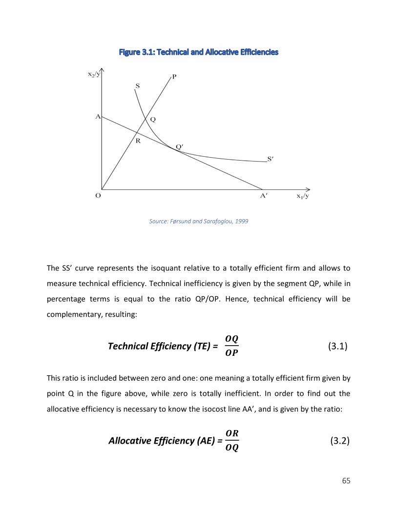
65

Figure 3.1: Technical and Allocative Efficiencies

Source: Førsund and Sarafoglou, 1999

The SS’ curve represents the isoquant relative to a totally efficient firm and allows to

measure technical efficiency. Technical inefficiency is given by the segment QP, while in

percentage terms is equal to the ratio QP/OP. Hence, technical efficiency will be

complementary, resulting:

Technical Efficiency (TE) = 𝑶𝑸𝑶𝑷

(3.1)

This ratio is included between zero and one: one meaning a totally efficient firm given by

point Q in the figure above, while zero is totally inefficient. In order to find out the

allocative efficiency is necessary to know the isocost line AA’, and is given by the ratio:

Allocative Efficiency (AE) = 𝑶𝑹𝑶𝑸

(3.2)

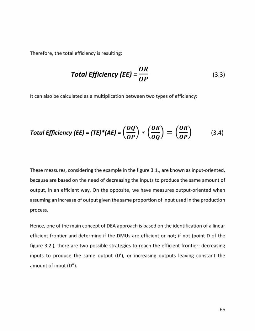
66

Therefore, the total efficiency is resulting:

Total Efficiency (EE) = 𝑶𝑹𝑶𝑷

(3.3)

It can also be calculated as a multiplication between two types of efficiency:

Total Efficiency (EE) = (TE)*(AE) = ~𝑶𝑸𝑶𝑷� ∗ ~𝑶𝑹

𝑶𝑸� = ~𝑶𝑹

𝑶𝑷� (3.4)

These measures, considering the example in the figure 3.1., are known as input-oriented,

because are based on the need of decreasing the inputs to produce the same amount of

output, in an efficient way. On the opposite, we have measures output-oriented when

assuming an increase of output given the same proportion of input used in the production

process.

Hence, one of the main concept of DEA approach is based on the identification of a linear

efficient frontier and determine if the DMUs are efficient or not; if not (point D of the

figure 3.2.), there are two possible strategies to reach the efficient frontier: decreasing

inputs to produce the same output (D’), or increasing outputs leaving constant the

amount of input (D”).

67

Figure 3.2: Efficient Frontier

Source: Gregoriou, Zhu, 2005

The DMUs that don’t need an increase of outputs, or a decrease of inputs, are located

on the efficient frontier. As a consequence, input-oriented models will optimize (reduce)

inputs with constant outputs level; vice versa, output-oriented models will optimize

(increase) outputs with constant inputs level. DEA gives information about DMUs’

efficiency and provides advice regarding not efficient DMUs; in addition, DEA also

provide suggestions about the variation of input (or output) required to enhance

performances. For these reasons, DEA models is considered an unbiased benchmarking

tool59.

59 G. N. Gregoriou, K. Sedzro, J. Zhu, Hedge Fund Performance Appraisal Using Data Envelopment Analysis, (2005).

68

DEA Basic Models

In this paragraph will be described three generic DEA models: CCR, BCC, and Allocative

models. Charnes, Cooper and Rhodes, the three authors behind the CCR model, at the

beginning of 70’s, started working on the evaluation process of educational program for

underprivileged public U.S. school students (i.e. black and Hispanic students). At the

beginning Cooper and Rhodes designed a model capable of identifying inefficiencies of

any input/output of DMUs; later on, Charnes expressed it formulaically from a

mathematical point of view and extended the approach to the efficiency measurement,

in order to be used in other fields and sectors. DEA methodology had an incredible rapid

development and has been immediately accepted due to its peculiarities and wide

applicability. Researchers from various sectors acknowledged DEA as valuable method for

operating processes modeling; its empirical nature and assumptions’ minimization lead

the application of DEA in many studies on the efficient frontier for what concerns no profit

organization in regulatory and private sectors. Now, we are going to analytically deal with

the first of the DEA basic models: CCR model.

CCR Model

Assuming n DMUs under valuation, is necessary to present four DMU’s selection criteria:

§ Positive numerical data available for every input and output considered

§ The choice regarding DMU, input and output must match manager’s interest

about DMU efficiency

§ Usually, small amount of input and large amount of output are preferred

69

§ No required consistency between data; can be compared different type of

input/output data.

Each DMU uses a given amount of m input to produce s output, with the properties stated

in the first 2 selection criteria. This relation can be written in matrix form with (X) as input

and (Y) as output:

For each DMU, Charnes, Cooper and Rhodes determined the virtual input with weight (ui)

and virtual output with weight (vr):

virtualinput=v1x1o+…+vmxmo (3.5)

70

𝒗𝒊𝒓𝒕𝒖𝒂𝒍𝒐𝒖𝒕𝒑𝒖𝒕 = u1𝒚1o+…+usyso (3.6)

Then, they calculated the weights, through linear programming, in order to maximize

the following ratio:

𝒗𝒊𝒓𝒕𝒖𝒂𝒍𝒐𝒖𝒕𝒑𝒖𝒕𝒗𝒊𝒓𝒕𝒖𝒂𝒍𝒊𝒏𝒑𝒖𝒕

(3.7)

The weights, as it has already been stated when describing peculiarities of DEA approach,

are derived from data instead of being assumed in advance. Once data have been chosen,

it’s time to evaluate the efficiency of each DMUs, hence n optimizations are necessary,

each for every DMUs. Going through the following fractional programming (FP) problem,

is possible to obtain input’s weights (ui) (i=1, ..., m) and output’s weights (vr) (r=1, …, s) as

variables:

FP0 𝒎𝒂𝒙𝒗,𝒖

𝜽 = 𝒖1𝒚1o�𝒖2𝒚2o�⋯�𝒖s𝒚s0𝒗1𝒙1o�𝒗2𝒙2o�⋯�𝒗m𝒙m0

(3.8)

Subject to:

�1�1j�⋯��s�sj�1�1j�⋯��m�mj

≤ 1(𝑗 = 1,… , 𝑛)(3.9)

𝑣1, 𝑣2, …, 𝑣𝑚 ≥ 0 (3.10)

𝑢1, 𝑢2,…,𝑢s ≥ 0(3.11)

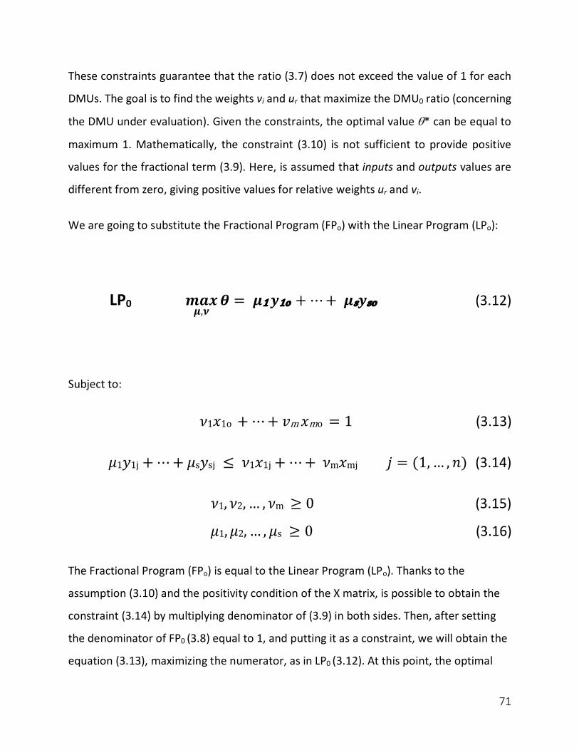
71

These constraints guarantee that the ratio (3.7) does not exceed the value of 1 for each

DMUs. The goal is to find the weights vi and ur that maximize the DMU0 ratio (concerning

the DMU under evaluation). Given the constraints, the optimal value q* can be equal to

maximum 1. Mathematically, the constraint (3.10) is not sufficient to provide positive

values for the fractional term (3.9). Here, is assumed that inputs and outputs values are

different from zero, giving positive values for relative weights ur and vi.

We are going to substitute the Fractional Program (FPo) with the Linear Program (LPo):

LP0 𝒎𝒂𝒙𝝁,𝝂

𝜽 = 𝝁1𝒚1o + ⋯+ 𝝁s𝒚so (3.12)

Subject to:

𝜈1𝑥1o + ⋯+ 𝑣m𝑥mo = 1 (3.13)

𝜇1𝑦1j + ⋯+ 𝜇s𝑦sj ≤ 𝜈1𝑥1j + ⋯+ 𝜈m𝑥mj 𝑗 = (1, … , 𝑛) (3.14)

𝜈1, 𝜈2,… , 𝜈m ≥ 0 (3.15)

𝜇1, 𝜇2, … , 𝜇s ≥ 0 (3.16)

The Fractional Program (FPo) is equal to the Linear Program (LPo). Thanks to the

assumption (3.10) and the positivity condition of the X matrix, is possible to obtain the

constraint (3.14) by multiplying denominator of (3.9) in both sides. Then, after setting

the denominator of FP0 (3.8) equal to 1, and putting it as a constraint, we will obtain the

equation (3.13), maximizing the numerator, as in LP0 (3.12). At this point, the optimal

72

solution of LPo is (n=n* and µ=µ*) and q* is the optimal objective value. The solution

(n=n* and µ=µ*) is also optimal for (FPo) and (LPo) therefore have the same optimal

solution q*.

Hence, the DMUo is CCR-efficient if q* = 1 and if exists at least one optimal solution (n*,

u*), with n*> 0 and u*> 0; in all other cases DMU0 is CCR-inefficient. Inefficiency, with

the CCR model, can have two meanings: on one hand that q* < 1, on the other hand q*

= 1 and at least one element from (n*, u*) is equal to 0 for each optimal solution of LPo.

Now we observe the case where DMUo has q* < 1 (CCR-inefficient). There must be at

least one DMU in constraint (3.14) for which the weight (n*, u*) gives the same results

in both sides, otherwise, q* coul be intensified. We will have:

𝐸 o = {j ∶ ∑ ur£¤q¥ *yrj= ∑ 𝜈i*¦

§q¥ 𝑥ij} (3.17)

The subset of DMUj that satisfies the previous equation is called reference set or peer

group to the DMU0, because they are on the efficient frontier representing the objective

for obtaining efficiency.

The optimal solution (n*, u*) obtained for LPo results in a series of optimal weights for

the DMU0. The q* can also be found with the following ratio:

𝜽* = ∑ u*r𝒚ro𝒔𝒓ª𝟏∑ 𝝂*𝒎𝒊ª𝟏 i𝒙io

(3.18)

From (3.13), the denominator is equal to 1 so:

73

∑ 𝜈*i𝑥i0 = 1¦§q¥ (3.19)

hence the optimal value q* can be rewritten as follows:

𝜽*=∑ 𝒖*𝒔𝒓q𝟏 r𝒚r0 (3.20)

The (3.19) is useful to define the relation, expressed in weight percentage, of an input

compared to the others, for each DMUs. While the (3.20) gives a measure of the

contribution of each output over the total efficiency.

Can be useful provide some analytical examples to understand the mechanism of this

model

Example 1 (1 input and 1 output):

Table 3.1:

DMU A B C D E F G H

Input 2 3 3 4 5 5 6 8

Output 1 3 2 3 4 2 3 5

Source: Cooper, Seiford, Tone, 2005

It is possible to calculate DMU A efficiency solving the following linear program problem:

A: max 𝜃 = 𝑢

Subject to:

2n = 1

74

u ≤ 2𝑣 (A) 3u ≤ 3𝑣 (B)

2u ≤ 3𝑣 (C) 3u ≤ 4𝑣 (D)

4u ≤ 5𝑣 (E) 2u ≤ 5𝑣 (F)

3u ≤ 6𝑣 (G) 5u ≤ 8𝑣 (H)

The optimal solution is the following: n*= 0.5, u*= 0.5, q*= 0.5. DMU A is not efficient,

because q* is lower than 1.

Do the same procedure to measure efficiency of DMU B:

B: max 𝜃 = 3𝑢

Subject to:

3n = 1

u ≤ 2𝑣 (A) 3u ≤ 3𝑣 (B)

2u ≤ 3𝑣 (C) 3u ≤ 4𝑣 (D)

4u ≤ 5𝑣 (E) 2u ≤ 5𝑣 (F)

3u ≤ 6𝑣 (G) 5u ≤ 8𝑣 (H)

Solving the problem, the optimal solution will be: n*= 0.333, u*= 0.333, q*= 1. B is CCR-

efficient. Then, repeating the same procedure for all the DMUs we obtain the following

table:

Table 3.2:

DMU v* u* q*

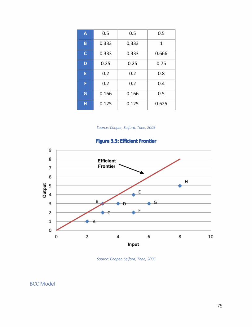
75

A 0.5 0.5 0.5

B 0.333 0.333 1

C 0.333 0.333 0.666

D 0.25 0.25 0.75

E 0.2 0.2 0.8

F 0.2 0.2 0.4

G 0.166 0.166 0.5

H 0.125 0.125 0.625

Source: Cooper, Seiford, Tone, 2005

Figure 3.3: Efficient Frontier

Source: Cooper, Seiford, Tone, 2005

BCC Model

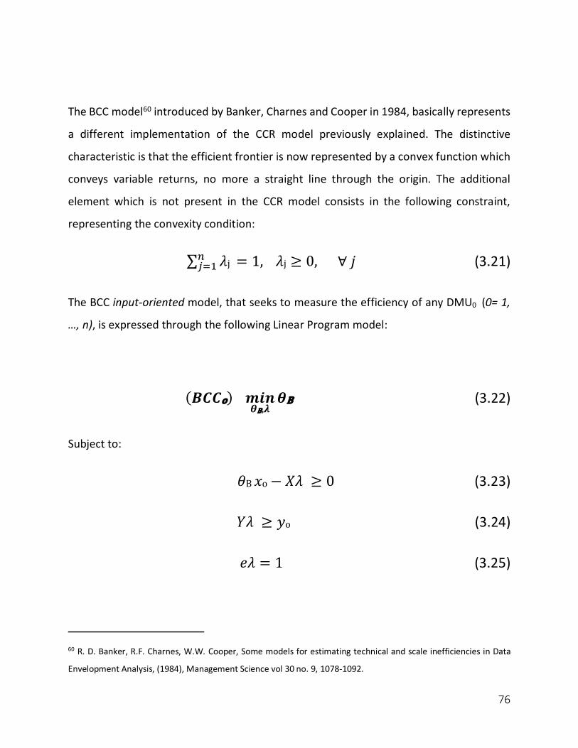
76

The BCC model60 introduced by Banker, Charnes and Cooper in 1984, basically represents

a different implementation of the CCR model previously explained. The distinctive

characteristic is that the efficient frontier is now represented by a convex function which

conveys variable returns, no more a straight line through the origin. The additional

element which is not present in the CCR model consists in the following constraint,

representing the convexity condition:

∑ 𝜆j = 1,² q¥ 𝜆j ≥ 0,∀𝑗 (3.21)

The BCC input-oriented model, that seeks to measure the efficiency of any DMU0 (0= 1,

…, n), is expressed through the following Linear Program model:

(𝑩𝑪𝑪o)𝒎𝒊𝒏𝜽B,𝝀

𝜽B (3.22)

Subject to:

𝜃B𝑥o − 𝑋𝜆 ≥ 0 (3.23)

𝑌𝜆 ≥ 𝑦o (3.24)

𝑒𝜆 = 1 (3.25)

60 R. D. Banker, R.F. Charnes, W.W. Cooper, Some models for estimating technical and scale inefficiencies in Data

Envelopment Analysis, (1984), Management Science vol 30 no. 9, 1078-1092.

77

𝜆 ≥ 0 (3.26)

Where qB is a scalar and (3.25) is the convexity condition. The dual multiplier form of the

(3.22) is the following:

𝒎𝒂𝒙𝝂,𝒖,𝒖0

𝒛 = 𝒖𝒚o − 𝒖o (3.27)

Subject to:

𝜈𝑥0 = 1 (3.28)

−𝜈𝑋 + 𝑢𝑌 − 𝑢0𝑒 ≤ 0 (3.29)

𝜈 ≥ 0,𝑢 ≥ 0 (3.30)

Where n and u are vectors, while z and uo are scalars, with uo may be positive or negative

(or zero).

The equivalent BCC fractional program can be obtained from the (3.27) as:

(𝑩𝑪𝑪 − 𝑶o)𝒎𝒂𝒙𝝂,𝒖

𝜽B = 𝒖𝒚oL𝒖o𝝂𝒙o (3.31)

Subject to:

𝑢𝑦jL�o»�j

≤ 1,𝑗 = 1,… , 𝑛 (3.32)

78

𝜈 ≥ 0,𝑢 ≥ 0 (3.33)

The first problem (BCC0) is solved with a two-phase procedure, similar to the one used for

CCR model. In the first phase, 𝜃B is minimized while in the second is maximized the sum

of the input excesses and output shortfalls. The optimal solution will be given by (𝜃*B, l*,

s-*, s+*), where s-* and s+* are called slacks and represent maximum input excesses and

output shortfalls, respectively. The optimal solutions satisfying 𝜃*B = 1 and has no slacks

(s-*= 0 and s+*= 0), is BCC-efficient, otherwise it is BCC-inefficient.

The BCC output-oriented model is defined as:

𝒎𝒂𝒙𝜼𝑩,½

𝜼B (3.34)

Subject to:

𝑋𝜆 ≤ 𝑥0 (3.35)

𝜂B𝑦0 − 𝑌𝜆 ≤ 0 (3.36)

𝑒𝜆 = 1 (3.37)

𝜆 ≥ 0 (3.38)

The dual form linked to the linear program (3.34) is expresses as:

𝒎𝒊𝒏𝝂,𝒖,𝝂¿

𝒛 = 𝝂𝒙0 - n0 (3.39)

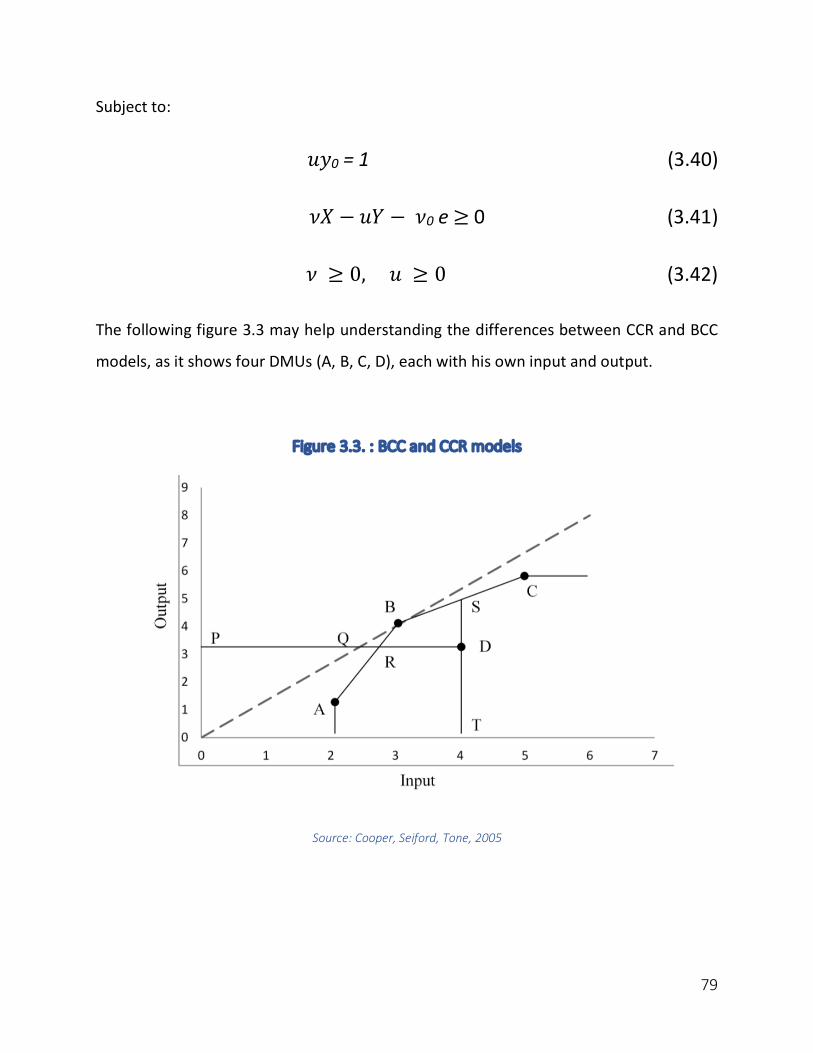
79

Subject to:

𝑢𝑦0 = 1 (3.40)

𝜈𝑋 − 𝑢𝑌 − 𝜈0 e ≥ 0 (3.41)

𝜈 ≥ 0,𝑢 ≥ 0 (3.42)

The following figure 3.3 may help understanding the differences between CCR and BCC

models, as it shows four DMUs (A, B, C, D), each with his own input and output.

Figure 3.3. : BCC and CCR models

Source: Cooper, Seiford, Tone, 2005

80

The CCR efficient frontier is the dotted line passing through the origin: it is clear that only

the DMU B is CCR-efficient, lying on the CCR efficient frontier. Instead, the BCC efficient

frontier is the broken line ABC. In this case DMUs A, B and C are BCC-efficient. Trying to

measure the efficiency of the DMU D, we notice that CCR and BCC models provide

different results: CCR-efficiency will be given by the ratio PQ/PD, while BCC-efficiency by

PR/PD. In addition, graphically we can note that the DMU D is less efficient under the CCR

model rather than the BCC; hence we can conclude that, generally speaking, CCR-

efficiency never exceeds BCC-efficiency.

Figure 3.4: Production Frontier with CCR (left) and BCC (right) models:

Source: Cooper, Seiford, Tone, (2005).

Additive Model

The Additive model was introduced by a group of scholars in 198561 and has the

predominant characteristic that there is no distinction between input and output-oriented

61 A. Charnes, W.W. Cooper, B. Golany, L. Seiford, J. Stutz, Foundations of data envelopment analysis for Pareto-

Koopmans efficient empirical production functions, (1985), Journal of Econometrics vol. 30, 91-107.

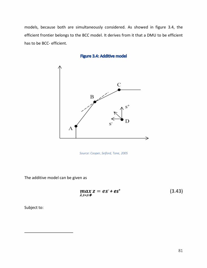
81

models, because both are simultaneously considered. As showed in figure 3.4, the

efficient frontier belongs to the BCC model. It derives from it that a DMU to be efficient

has to be BCC- efficient.

Figure 3.4: Additive model

Source: Cooper, Seiford, Tone, 2005

The additive model can be given as

𝒎𝒂𝒙𝝀,𝒔-,𝒔�

𝒛 = 𝒆𝒔- + es+ (3.43)

Subject to:

82

𝑋𝜆 + 𝑠- = x0 (3.44)

𝑌𝜆 − 𝑠+ = y0 (3.45)

𝑒𝜆 = 1 (3.46)

𝜆 ≥ 0,𝑠- ≥ 0, 𝑠+≥ 0 (3.47)

Where s- and s+ represent output and input slacks. This model considers the total slacks

simultaneously in arriving at a point on the efficient frontier.

The dual problem to the additive model (3.43) can be expressed as follows:

𝒎𝒊𝒏𝝂,𝒖,𝒖𝟎

𝒘 = 𝝂𝒙0 – uy0 + u0 (3.48)

Subject to:

𝜈𝑋 − 𝑢𝑌 + 𝑢0 e ≥ 0 (3.49)

𝜈 ≥ 𝑒 (3.50)

𝑢 ≥ 𝑒 (3.51)

83

The optimal solution is given by (l*, s-*, s+*) and any DMU0 to be efficient must respect

the following conditions: s-*= 0 and s+*= 062.

The application of DEA can be a very powerful tool whether used wisely. Those that

follow are some of the advantages of DEA approach. First of all, it is a tool that can

handle multiple inputs and outputs models, using a unique total efficiency measure,

without any weighting factors63. DMUs are directly compared against peer or

combination of peers. DEA does not require an assumption of a functional form

concerning inputs to outputs. Finally, contrary to other models, in order to analyze DMU

efficiency, inputs and outputs may have different units, given that DEA is not limited to

monetary units64.

Though, the same features that make DEA so useful, can also be reflected in weaknesses

of analysis. When choosing to adopt DEA model, is necessary to keep in mind the

following limitations: DEA is a useful tool to measure relative efficiency, but when it

comes to evaluate absolute efficiency it is not so powerful tool, meaning that it is the

right technique if you want to know how well you are doing compared to a peer or a

group of peers, but not compared to the theoretical maximum. Large problems can be

computational intensive, requiring time and powerful calculation machines.

62 W. W. Cooper, L. M. Seiford, K. Tone, Introduction to Data Envelopment Analysis and its uses: with DEA-Solver

software and references, (2005), Springer-Verlag. 63 W. P. Fox, Mathematical Modeling for Business Analytics, (2017), CRC Press. 64 N. Johns, B. Howcroft, L. Drake, The use of data envelopment analysis to monitor hotel productivity, (1997),

Progress in Tourism and Hospitality Research.

84

Application DEA Models for Investment Funds Evaluation

In this chapter we are going to describe some models that, through DEA technique, have

been used to measure and analyze the efficiency of investment funds. Most of the

traditional risk-adjusted measures, on one hand are very helpful in providing simple and

immediate results in clear and comparable terms, but on the other hand are unsuitable

for a correct and complete performance valuation of mutual funds, due to the fact, as

already stated, that they don’t take in consideration fees and expenses investors have to

bear (measured with expense ratio). For this reason, scholars started to apply DEA for

mutual funds analysis, with the goal to find an efficiency measure as complete and

objective as possible.

Murthi, Choi and Desai Model

Murthi, Choi and Desai model (1997)65 was the first approach to the performance

evaluation of mutual funds through the DEA. At the heart of this model, there is the

critics to traditional measures, especially Sharpe ratio and Jensen alpha, because, as far

as they were concerned, these metrics caused many problems. From Jensen’s alpha

they complaint the choice of correct benchmark, that is based on theories such as CAPM

or APT, that are considerably outdated due to their strong underlying assumptions. The

65 B. P. S. Murthi, Y. K. Choi, P. Desai, Efficiency of mutual funds and portfolio performance measurement: a non-

parametric approach, European Journal of Operational Research vol. 98, (1997).

85

weak point of both Jensen’s alpha and Sharpe ratio, instead, consists in the fact that

they do not consider the weight of transaction costs66. In order to include these costs in

their model, Murthi, Choi and Desai created a new innovative index, modifying the

original Sharpe ratio with the addition of transaction fees and expenses. This new

measure is called DEA Portfolio Efficiency Index (DPEI), formulated as:

𝑫𝑷𝑬𝑰 = 𝑹0∑ 𝒘ixio�𝝂𝝈o𝒍𝒊ª𝟏

(3.52)

Subject to:

ÄÅ∑ Æixij�»ÇjÈɪÊ

≤ 1𝑗 = 1,… , 𝐽 (3.53)

𝑤i ≥ 𝜀,𝜈 ≥ 𝜀 (3.54)

Where J is the number of funds of the same category, l is the inputs’ number, Rj

describes the average return of jth fund, xIJ is the transaction cost value (i) for the jth

fund, wi and n are the weights associated to xi and wi variables respectively, sj is the

standard deviation of the jth fund and e is a constant number. To calculate the index

(DPEI), they applied DEA, solving an optimization problem that defines optimal weights

and efficiency level of a fund.

The reasons why the authors chose to apply DEA are the following:

66 Generally called transaction costs, meaning all those fees and expenses that investors have to bear when buying,

holding and selling investment funds’ shares.

86

- It does not require benchmarks, it just measures the best performance of a

mutual fund compared to a group of funds of the same category.

- It takes in consideration, in a unique analysis, the expected return of a fund and

relative transaction costs, such as expense ratio, turnover index and other fees.

DPEI is flexible and can use a lot of inputs and outputs in measuring the

performance.

- It can monitor marginal contribution of each input on the total performance,

reallocating in this way resources in a timely and efficient way.

When it comes to provide a judgement about the performance of a given portfolio, it

has to be included in the evaluation process also the cost component, because investors

look for returns’ maximization together with costs’ minimization.

Here, Murthi, Choi and Desai chose one output variable, the return, and four input

variables: total expense ratio (TER), loads, switch commissions67 and standard deviation.

Therefore, through the application of DEA is possible to find the weights that maximize

the return of a fund, based on their inputs, hold in mind that the relation (3.52) has to

be less or equal to 1 for each fund, and the weights must be positive values.

Remembering that DEA method are used to measure a fund’s efficiency relative to a

bunch of funds sharing the identical inputs to obtain the same outputs. The distance of

inefficient funds from the frontier represents the measure of fund’s inefficiency.

67 Switch fee is the charge collected by a fund management group when an investor moves money from one fund to

another.

87

In the DPEI index, a mutual fund has to be considered efficient when the function (3.52)

is equal to 1 and all the slacks are equal to 0; while it will be inefficient only when

compared with other funds in the model.

Murthi, Choe and Desai, analyzed more than two thousand mutual funds from the third

quarter of 1993 dividing in 7 sub-categories,68 classified by funds’ strategies. The results

are compared to the Jensen’s alpha and Sharpe ratio, calculating the correlation. The

three authors discovered the presence of a positive correlation between DPEI and both

Sharpe ratio and Jensen’s alpha for all the fund’s categories, meaning that DPEI is

consistent with traditional risk-adjusted measures, though offering, at the same time,

greater flexibility.

Finally, they calculated the correlation index between funds’ ranking based on NAV69

and the one based on DEA results, in order to measure the effect of fund’size on the

total efficiency: they found for some fund’s categories a positive correlation. This result

was justified with the fact that larger funds could be more efficient due to lower weight

of transaction costs.

To conclude, these studies demonstrate that DEA technique is appropriate for

evaluating efficiency of mutual funds, more flexible than traditional methods, thanks to

the freedom of choice about inputs and outputs.

Basso and Funari Model

68 The categories are: growth, growth income, aggressive growth, balanced, asset allocation, income, equity income.

From the results appear that the best ones were: aggressive growth, asset allocation, income and equity income

while the remaining three had low efficiency’s level. 69 For the definition of Net Asset Value, check the Chapter 1, paragraph “Open-end Funds”.

88

Basso and Funari model (2001)70 can be intended as a generalization of Murthi, Choi and

Desai model (1997), allowing to take in consideration various risk measures. The

difference between Basso and Funari and his predecessor model, consists in the fact

that they used a different index, named IDEA_1, which, unlike the one proposed by

Murthi, Choi and Desai, considers among input variables, only direct fees at the expense

of the investor, that is to say submission and redemption costs, leaving out other

indirect costs, such as operative expenses and management commissions. This because

the historical series of data about funds’ returns are net of those “indirect costs”.

Hence, the measure proposed, IDEA_1, can be obtained solving the following linear

problem:

𝐦𝐚𝐱{𝒖,𝝂j,𝒘i}

𝒖𝒐j0∑ 𝝂i𝒒ij0�∑ 𝒘i𝒄ij0𝒌

𝒊ª𝟏𝒉𝒊ª𝟏

(3.55)

Subject to:

�Ój∑ »iÔij�∑ ÆiÕijÖ

ɪÊ×ɪÊ

≤ 1,𝑗 = 1,… , 𝑛 (3.56)

𝑢 ≥ 𝜀

𝜈i ≥ 𝜀, i = 1, …, h

𝑤i ≥ 𝜀,𝑖 = 1,…, k

70 A. Basso, S. Funari, A data envelopment analysis approach to measure the mutual fund performance, European

Journal of Operational Research, (2001).

89

Where u is the outuput weight, n is the input weight, while j represents a generic fund, k

is the costs’ number under consideration (cij) and h is the number of risks’ measures (qij).

Therefore, they used the fund’s return as the output of the model, while four different

inputs, as measures of risk:

§ Standard deviation of returns

§ Beta coefficient (b) of a reasonable benchmark71

§ % Subscription costs

§ Redemption costs (relative to different time horizon 1-2-3 years)

In addition, Basso and Funari developed an indicator of stochastic dominance reflecting

the percentage of sub-periods, compared to the evaluation time horizon, by which a

fund is not dominated by other funds. It will be expressed with the dj as a certification of

the validity of a fund as time goes by. With this gauge, they developed a different DEA

measure, IDEA_2, characterized by two outputs, which can be defined as:

𝒖1𝒐j0�𝒖2𝒅j0∑ 𝝂i𝒒ij0�∑ 𝒘i𝒄ij0𝒌

𝒊ª𝟏𝒉𝒊ª𝟏

(3.57)

Subject to:

�1Ój��2Új∑ »iÔij�∑ ÆiÕijÖ

ɪÊ×ɪÊ

≤ 1,𝑗 = 1,… , 𝑛 (3.58)

𝑢r≥ 𝜀,𝑟 = 1, 2

𝜈i ≥ 𝜀,𝑖 = 1, … , ℎ

71 As market portfolio benchmark Basso and Funari considered the Mibtel index.

90

𝑤i ≥ 𝜀,𝑖 = 1, … , 𝑘

Basso and Funari analyzed 47 Italian mutual funds, divided by investment categories

(equity, bond and balanced)72, for the period between 1st January 1997 and 30th June

1999.

The procedure allows to identify, for each inefficient fund, a series of equivalent

efficient funds as benchmarks. The method highlighted the importance of underwriting

and redemption fees when comparing and evaluating mutual funds. Moreover, applying

the gauge IDEA_2 the results don’t change very much, rather, with this approach it comes

up a higher number of efficient funds.

To conclude, results of the application of the Basso and Funari approach suggests that

the DEA method can be very helpful in the mutual fund efficiency evaluation, in addition

to traditional risk-adjusted measures. Comparing results from DEA with traditional

performance metrics, such as Sharpe, Treynor ratios and Jensen’s alpha, it shows low

correlations: this meaning that fees and, generally speaking, transaction costs, are not

taken in consideration in traditional measurements, with the possibility of

compromising the total performance judgement of investments.

Morey and Morey Model

72 For the categorization of mutual funds, was used the criteria adopted by Assogestioni:

http://www.assogestioni.it/index.cfm/1,132,0,49,html/elenco-fondi

91

Morey and Morey73 based their work on a simple consideration: most investors put

their savings in mutual funds, selecting among them looking at ratings. Morey and

Morey developed two alternative methods for mutual funds ratings’ measurement in

such a way as to provide additional information about risk and return, from an objective

perspective. Through these approaches is possible to verify if a fund lies on the efficient

frontier or not. The approach shares the following features:

- Non-parametric methods

- Transparent approaches, giving final ratings with clear economic interpretations

- Each mutual fund is evaluated compared to an endogenous benchmark fund, ad

hoc created, running during the same period.

- Provide, for underperforming funds, levels of risk and returns necessaries to

reach the efficient frontier

In the first method, the attention is addressed to simultaneous increase of average

returns, over the entire time horizon, maintaining the same level of total risk in each

period. (Total risk includes systemic risk, beta). With the second method, designing a

different benchmark fund, endogenously produced, the goal is to reduce,

simultaneously, total risk through the whole time frame, without affecting average

return.

First approach determines wj ≥ 0 and q ≥ 1 so:

𝐦𝐚𝐱𝜽 (3.59)

73 M. R. Morey, R. C. Morey, Mutual fund performance appraisals: a multi- horizon perspective with endogenous

benchmarking, Omega, The International Journal of Management Science vol. 27, (1998).

92

Subject to:

∑ 𝑤Þ q¥ j = 1 (3.60)

∑ 𝑤Þ q¥

2js2

j,t + ∑ ∑ 𝑤Þ q¥

Þ§q¥ iwj Cov (Ri,t, Rj,t) ≤ 𝜎2

j0,t (t=1, …, T)

∑ 𝑤Þ q¥ j E(Rj,t) ≥ 𝜃𝐸(𝑅j0,t) (t=1, …, T) (3.62)

where j is the number (between 1 and N) of funds to evaluate, T is the number of

different time period considered; Rj,t represents a random variable; E(Rj,t) is the mean,

s2j,t is the variance and Cov(Ri,t, Rj,t) are the covariances.

This method is useful because allows to assign an objective rating to mutual fund based

on its distance from the efficient frontier; however, it requires prudence when using q*

for rating the performances of mutual funds, due to the nature of the model.

The second approach is the following:

𝐦𝐢𝐧𝒁 (3.63)

Subject to:

∑ 𝑤Þ q¥ j = 1 (3.64)

∑ 𝑤Þ q¥ j E(Rj,t) ≥ 𝐸(𝑅j0,t) (t=1, …, T) (3.65)

∑ 𝑤Þ q¥

2js2

j,t + ∑ ∑ 𝑤Þ q¥

Þ§q¥ jwi Cov(Ri,t, Rj,t) ≤ 𝑍𝜎2

j0,t (t=1, …, T) (3.66)

93

Morey and Morey analyzed 26 mutual funds, from “aggressive growth” Morningstar

category, selecting monthly data, for 10 years. For each fund they calculated the

monthly mean, and 3 ,5 and 10 years variance and covariance, then applied both

approaches depicted above, using as inputs variables the variance return and

correlation between funds’ returns, for each period under evaluation.

The results showed eight funds lying on the efficient frontier while the remaining 18

funds were not. Finally, they ranked those eight efficient funds.

Gregoriou, Sedzro and Zhu Model

Gregoriou, Sedzro and Zhu (2004)74 developed a DEA model for hedge funds’75

evaluation. Due to the nature and objective of hedge funds, that seek to maximize

returns without any benchmark comparison, there was the need for an evaluation

method which satisfies these requirements. Hedge funds show different characteristics

about returns, if related to mutual funds, therefore applying traditional risk-adjusted

measures for the valuation may provide misleading and unreliable results. Especially,

74 Gregariou G. N., Sedzro K., Zhu J. (2004), Hedge fund performance appraisal using data envelopment analysis,

European Journal of Operational Research. 75 A hedge fund is an alternative investment vehicle available only to sophisticated investors, such as institutions and

individuals with significant assets. Like mutual funds, hedge funds are pools of underlying securities, and can invest

in many types of securities. But contrary to mutual funds, hedge funds are not regulated by the SEC (in U.S.), while

in Europe are regulated by the AIFM.

94

due to the asymmetric nature returns, the application of Sharpe ratio would provide

inappropriate results.

Three are the input variables applied in this model: lower mean monthly semi-skewness

(LSS), lower mean monthly semi-variance (LSV), and mean monthly lower return (MLR).

DEA model used is BCC: Gregoriou, Sedzro and Zhu then compared results from DEA

with the Modified Sharpe Ratio (MSR), that is the following:

MSR = 𝑹𝐩𝐭L𝑹𝐟

𝑾ç𝝁Lè𝒛𝐜�𝟏𝟔(𝒛𝟐𝐜L𝟏�𝑺� 𝟏𝟐𝟒í𝒛

𝟑𝐜L𝟑𝒛𝐜ï𝐊L 𝟏𝟑𝟔í𝟐𝒛𝟑𝐜L𝟓𝒛𝐜ï𝑺𝟐òs]

(3.67)

Where Rpt is the portfolio return, Rf is the risk-free rate (Treasury-Bill 30 days), Zc is the

value associated to the probability equal to (1-a), S is skewness and K is the kurtosis.

Then they calculated the modified VaR (Value at Risk)76, with the following formula:

zCF = zc + ¥ó (z2

c – 1) S + ¥ôõ

(z3c – 3zc) K - ¥

öó (2z3

c – 5zc) S2 (3.68)

Later, they used the Jarque-Bera test in order to verify the not normal nature of returns:

76 Valure at Risk is a measure of the risk of loss for investments. VaR is defined as the maximum possible loss during

the time, for a given portfolio, time horizon and probability p.

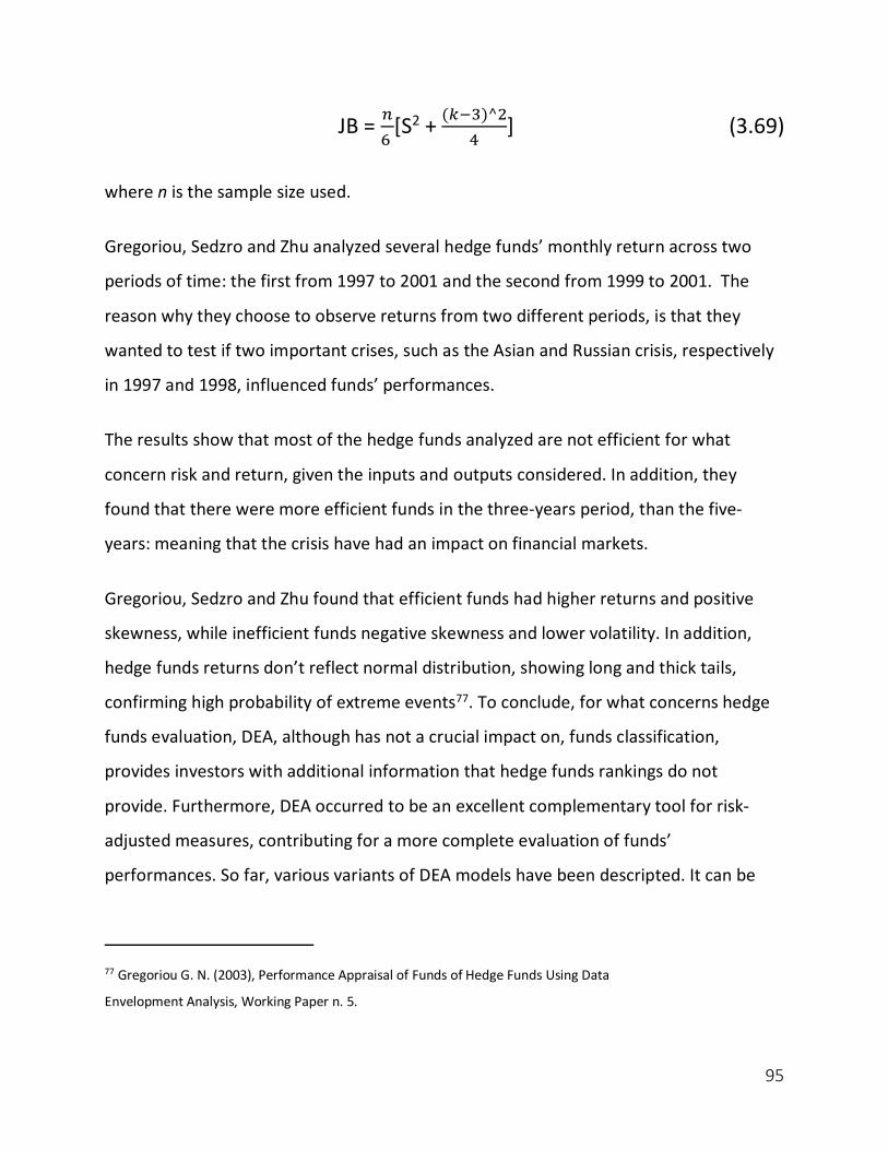
95

JB = ²ó

[S2 + (÷Lö)^ôõ

] (3.69)

where n is the sample size used.

Gregoriou, Sedzro and Zhu analyzed several hedge funds’ monthly return across two

periods of time: the first from 1997 to 2001 and the second from 1999 to 2001. The

reason why they choose to observe returns from two different periods, is that they

wanted to test if two important crises, such as the Asian and Russian crisis, respectively

in 1997 and 1998, influenced funds’ performances.

The results show that most of the hedge funds analyzed are not efficient for what

concern risk and return, given the inputs and outputs considered. In addition, they

found that there were more efficient funds in the three-years period, than the five-

years: meaning that the crisis have had an impact on financial markets.

Gregoriou, Sedzro and Zhu found that efficient funds had higher returns and positive

skewness, while inefficient funds negative skewness and lower volatility. In addition,

hedge funds returns don’t reflect normal distribution, showing long and thick tails,

confirming high probability of extreme events77. To conclude, for what concerns hedge

funds evaluation, DEA, although has not a crucial impact on, funds classification,

provides investors with additional information that hedge funds rankings do not

provide. Furthermore, DEA occurred to be an excellent complementary tool for risk-

adjusted measures, contributing for a more complete evaluation of funds’

performances. So far, various variants of DEA models have been descripted. It can be

77 Gregoriou G. N. (2003), Performance Appraisal of Funds of Hedge Funds Using Data

Envelopment Analysis, Working Paper n. 5.

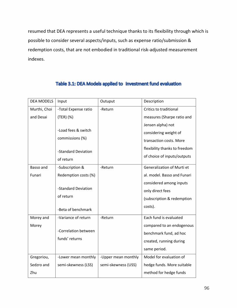
96

resumed that DEA represents a useful technique thanks to its flexibility through which is

possible to consider several aspects/inputs, such as expense ratio/submission &

redemption costs, that are not embodied in traditional risk-adjusted measurement

indexes.

Table 3.1: DEA Models applied to investment fund evaluation

DEA MODELS Input Outuput Description

Murthi, Choi

and Desai

-Total Expense ratio

(TER) (%)

-Load fees & switch

commissions (%)

-Standard Deviation

of return

-Return Critics to traditional

measures (Sharpe ratio and

Jensen alpha) not

considering weight of

transaction costs. More

flexibility thanks to freedom

of choice of inputs/outputs

Basso and

Funari

-Subscription &

Redemption costs (%)

-Standard Deviation

of return

-Beta of benchmark

-Return Generalization of Murti et

al. model. Basso and Funari

considered among inputs

only direct fees

(subscription & redemption

costs).

Morey and

Morey

-Variance of return

-Correlation between

funds’ returns

-Return

Each fund is evaluated

compared to an endogenous

benchmark fund, ad hoc

created, running during

same period.

Gregoriou,

Sedzro and

Zhu

-Lower mean monthly

semi-skewness (LSS)

-Upper mean monthly

semi-skewness (USS)

Model for evaluation of

hedge funds. More suitable

method for hedge funds

97

-Lower mean monthly

semi-variance (LSV)

-Mean monthly lower

return (MLR)

-Upper mean monthly

semi-variance (USV)

-Mean monthly upper

return (ULR)

returns not normal

distribution.

An Empirical Application of DEA approach:

Evaluation of Italian Mutual Funds

Introduction

In this chapter it will be described the application of a particular BCC-input oriented DEA

98

model used to evaluate the efficiency of a sample of Italian investment funds. Through

the use of a specific DEA model, it has been possible compute the efficiency for the

aforementioned sample, drawing up in this way a rank of performance efficiency, which

is compared with results based on traditional risk-adjusted metrics, such as Sharpe and

Sortino ratios, in order to evaluate the integrity of DEA model.

The evaluation and comparison processes are directed towards an empirical assessment

of transaction costs’ incidence over the total performance of mutual funds, incidence that

is not embedded in most used, and well-known, risk-adjusted measures. Through the

analysis of correlation, it will be investigated the degree of correlation, whether positive,

null or negative, between DEA results and traditional performance gauges, such as Sharpe

and Sortino ratio, and even size measure, as the asset under management (AUM). Finally,

it will be also compared DEA efficiency results with funds’ size, in order to appraise

whether there is a relation between performance and size. In the ensuing paragraph, it

will be presented sample of data, along with selection criteria, and methodology used to

perform the aforesaid analysis

Data sample and Methodology

In order to fulfill the analysis, starting from the specific application of DEA approach

conceived by Murthi, Choi and Desai78, from now on MCD, it will be assessed the

efficiency of selected cluster of investment funds, and in order to better observe the time

effect, it was decided to carry on two different analyses, related to different time

windows, one and three years. Based on the MCD method, the data sample has been

selected taking into consideration, firs of all, the availability of data required by the

specific model: obviously one of the fundamental feature that a sample has to have for

78 See Chapter 3.

99

be employed in DEA analysis is the homogeneity of data, along with the full accessibility

of a certain dataset. Data have been obtained from two different sources: principally

Bloomberg while, to a lesser extent, Morningstar.

As explained repeatedly across this work, it is well known that efficiency and performance

assessment focus mainly on risk and return gauges. Since the analysis must be done on a

consistent and homogeneous sample of data in order to have reliable results, we firstly

to set the selection criteria. The following are the ones used for this analysis: Italian79 mid

and large-cap mutual funds, with available data from December 2014 until January 2018.

Through the function Fund Screening, or FSCR, I applied the filters (as shown in Figure

4.1): “Italy”, “Date” and “AUM”. For what concerns the period, in order to have returns

and other risk factors related to one and three years, it has to be set a time window

starting from December 2014 ending on January 2018, with monthly frequency; while

regarding the assets managed by funds, it is necessary to fix a minimum amount of “AUM”

of €300 mln. Unfortunately, it was not possible to find data required for all the funds,

mainly due to the following reasons: part of them have been launched after 2014,

consequently there aren’t available data to run the model for both the time periods

considered; while other funds, presenting negative returns, cannot deal with DEA model.

Therefore, applying these filters on Bloomberg terminal, the sample of data was extracted

from the Bloomberg database, from which it is necessary to skim funds with negative

returns, after having calculated them.

Figure 4.1: Bloomberg function FSCR

79 Italy intended as “Country of Domicile”, as indicated on Bloomberg. All the available funds domiciliated, listed and

traded on the Italian Stock Exchange (Borsa Italiana).

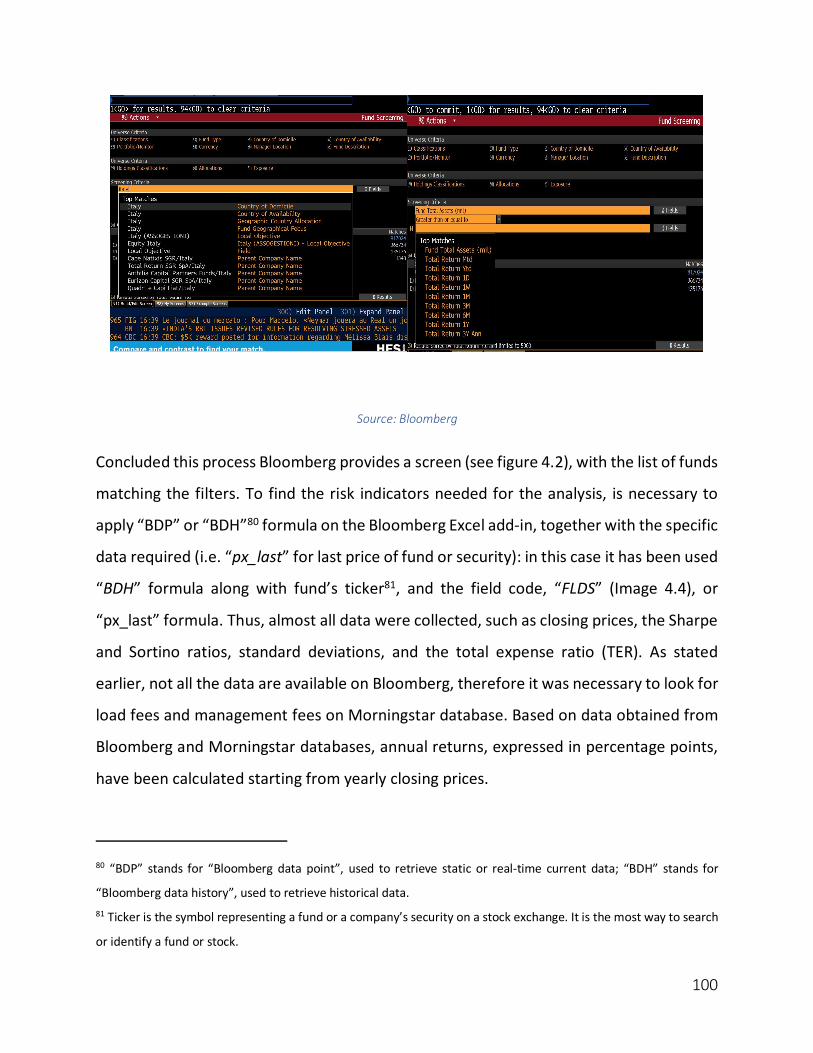
100

Source: Bloomberg

Concluded this process Bloomberg provides a screen (see figure 4.2), with the list of funds

matching the filters. To find the risk indicators needed for the analysis, is necessary to

apply “BDP” or “BDH”80 formula on the Bloomberg Excel add-in, together with the specific

data required (i.e. “px_last” for last price of fund or security): in this case it has been used

“BDH” formula along with fund’s ticker81, and the field code, “FLDS” (Image 4.4), or

“px_last” formula. Thus, almost all data were collected, such as closing prices, the Sharpe

and Sortino ratios, standard deviations, and the total expense ratio (TER). As stated

earlier, not all the data are available on Bloomberg, therefore it was necessary to look for

load fees and management fees on Morningstar database. Based on data obtained from

Bloomberg and Morningstar databases, annual returns, expressed in percentage points,

have been calculated starting from yearly closing prices.

80 “BDP” stands for “Bloomberg data point”, used to retrieve static or real-time current data; “BDH” stands for

“Bloomberg data history”, used to retrieve historical data. 81 Ticker is the symbol representing a fund or a company’s security on a stock exchange. It is the most way to search

or identify a fund or stock.

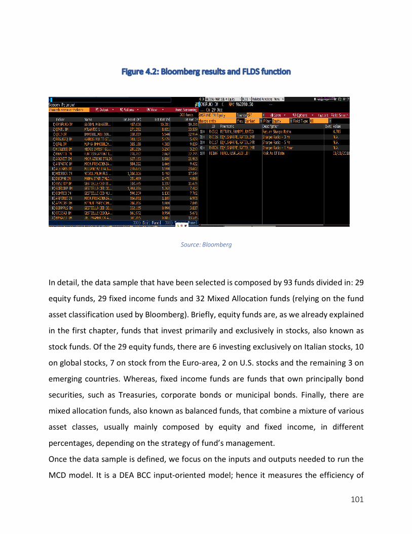
101

Figure 4.2: Bloomberg results and FLDS function

Source: Bloomberg

In detail, the data sample that have been selected is composed by 93 funds divided in: 29

equity funds, 29 fixed income funds and 32 Mixed Allocation funds (relying on the fund

asset classification used by Bloomberg). Briefly, equity funds are, as we already explained

in the first chapter, funds that invest primarily and exclusively in stocks, also known as

stock funds. Of the 29 equity funds, there are 6 investing exclusively on Italian stocks, 10

on global stocks, 7 on stock from the Euro-area, 2 on U.S. stocks and the remaining 3 on

emerging countries. Whereas, fixed income funds are funds that own principally bond

securities, such as Treasuries, corporate bonds or municipal bonds. Finally, there are

mixed allocation funds, also known as balanced funds, that combine a mixture of various

asset classes, usually mainly composed by equity and fixed income, in different

percentages, depending on the strategy of fund’s management.

Once the data sample is defined, we focus on the inputs and outputs needed to run the

MCD model. It is a DEA BCC input-oriented model; hence it measures the efficiency of

102

output over inputs, placing emphasis on reduction of certain inputs to improve efficiency.

In this case, as the three authors did in 1997, there are three inputs and one output. As

inputs, representing the volatility of returns there is the standard deviation, while the

remaining two inputs represent the so-called transaction costs: fees that an investor bear

when owning mutual fund shares; more precisely there are the total expense ratio (TER)82

and load fees. Unlike MCD model, there is no switch commissions among inputs, because

they are not available for the complete data sample under analysis. To conclude, as

output it has been used the annual funds’ return.

The following table summarizes the factors applied within the MCD model, along with

items’ description83:

Table 4.1: Inputs and Output used in DEA model

INPUT DESCRIPTION

82 For what concerns the TER, one of the most important cost are the management fees. 83 Definition given by Morningstar Investing Glossary:

http://www.morningstar.com/InvGlossary/expense_ratio.aspx

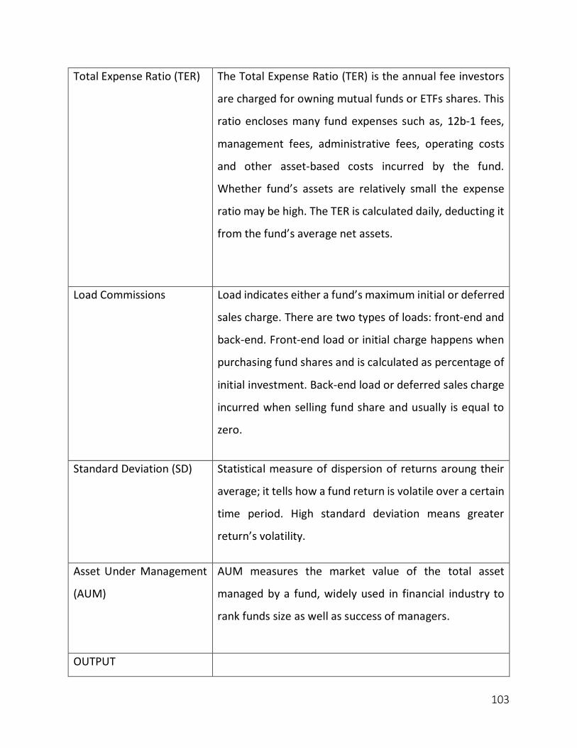
103

Total Expense Ratio (TER) The Total Expense Ratio (TER) is the annual fee investors

are charged for owning mutual funds or ETFs shares. This

ratio encloses many fund expenses such as, 12b-1 fees,

management fees, administrative fees, operating costs

and other asset-based costs incurred by the fund.

Whether fund’s assets are relatively small the expense

ratio may be high. The TER is calculated daily, deducting it

from the fund’s average net assets.

Load Commissions Load indicates either a fund’s maximum initial or deferred

sales charge. There are two types of loads: front-end and

back-end. Front-end load or initial charge happens when

purchasing fund shares and is calculated as percentage of

initial investment. Back-end load or deferred sales charge

incurred when selling fund share and usually is equal to

zero.

Standard Deviation (SD) Statistical measure of dispersion of returns aroung their

average; it tells how a fund return is volatile over a certain

time period. High standard deviation means greater

return’s volatility.

Asset Under Management

(AUM)

AUM measures the market value of the total asset

managed by a fund, widely used in financial industry to

rank funds size as well as success of managers.

OUTPUT

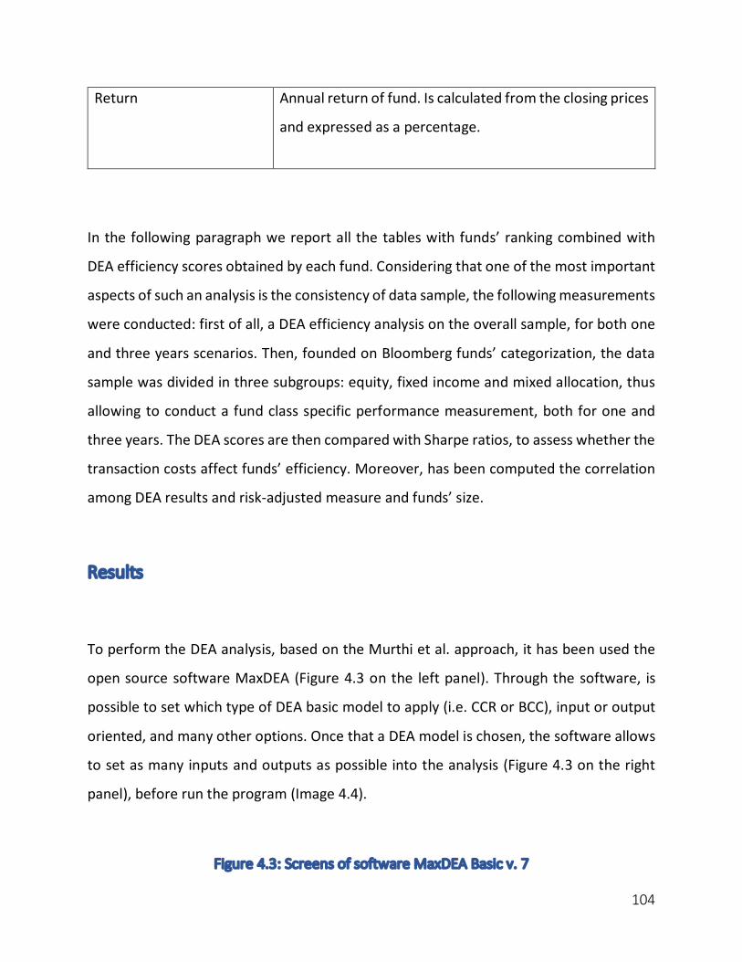
104

Return Annual return of fund. Is calculated from the closing prices

and expressed as a percentage.

In the following paragraph we report all the tables with funds’ ranking combined with

DEA efficiency scores obtained by each fund. Considering that one of the most important

aspects of such an analysis is the consistency of data sample, the following measurements

were conducted: first of all, a DEA efficiency analysis on the overall sample, for both one

and three years scenarios. Then, founded on Bloomberg funds’ categorization, the data

sample was divided in three subgroups: equity, fixed income and mixed allocation, thus

allowing to conduct a fund class specific performance measurement, both for one and

three years. The DEA scores are then compared with Sharpe ratios, to assess whether the

transaction costs affect funds’ efficiency. Moreover, has been computed the correlation

among DEA results and risk-adjusted measure and funds’ size.

Results

To perform the DEA analysis, based on the Murthi et al. approach, it has been used the

open source software MaxDEA (Figure 4.3 on the left panel). Through the software, is

possible to set which type of DEA basic model to apply (i.e. CCR or BCC), input or output

oriented, and many other options. Once that a DEA model is chosen, the software allows

to set as many inputs and outputs as possible into the analysis (Figure 4.3 on the right

panel), before run the program (Image 4.4).

Figure 4.3: Screens of software MaxDEA Basic v. 7

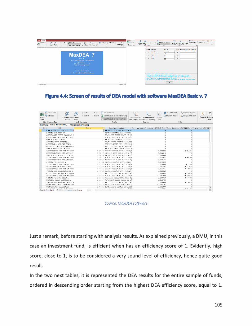
105

Figure 4.4: Screen of results of DEA model with software MaxDEA Basic v. 7

Source: MaxDEA software

Just a remark, before starting with analysis results. As explained previously, a DMU, in this

case an investment fund, is efficient when has an efficiency score of 1. Evidently, high

score, close to 1, is to be considered a very sound level of efficiency, hence quite good

result.

In the two next tables, it is represented the DEA results for the entire sample of funds,

ordered in descending order starting from the highest DEA efficiency score, equal to 1.

106

These two tables show respectively the results based on the 1 year, 2017, and 3-years

analysis; from the left there are: Fund name and category, DEA result, return, total

expense ratio, load fee, Sharpe ratio and standard deviation.

As it is clear from the first table (Table 4.2), efficient funds are 7 over 93, 4 fixed income,

2 equity and the remaining one mixed allocation fund. It can be noted that efficiency is

due to different reasons: great returns for two equity funds (i.e. “EURIZON AZIONI PMI

ITALIA” with 33.94%), very low volatility of returns, expressed by the standard deviation

(i.e. “EURIZON CEDOLA ATT OTT 2019” with 0.88), and very low level of transaction costs,

expressed by the sum of TER and loads (i.e. “ACOMEA BREVE TERMINE A-1” with 0.66%

of total fees).

Looking at the results showed in the second table (Table 4.3), concerning the 3-years

performance, it can be confirmed the reasons behind the funds’ efficiency. Indeed, there

are some funds with great returns over the three years, other funds showing low values

of standard deviation, and finally, some funds with very low level of transaction costs,

confirming the validity and usefulness of DEA.

Table 4.2: AllFunds DEA Efficiency Results 1Y

FUND NAME BLOOMBERG CATEGORY

DEA SCORE RETURN 1Y TER %

LOAD %

SHARPE 1Y SD 1Y

ACOMEA BREVE TERMINE-A1 Fixed Income 1 1.67% 0.66 0 1.27 1.44

ARCA AZIONI EUROPA Equity 1 10.43% 2.12 0 1.82 7.01

ARCA BOND PAESI EMERGENTI Fixed Income 1 7.13% 1.36 0 2.62 2.37

ARCA CED 2019 OBBLIG ATT V-P Fixed Income 1 0.20% 1 0 1.38 0.74

EURIZON AZIONI PMI ITALIA Equity 1 33.94% 2.1 1.5 2.44 13.46

EURIZON CEDOLA ATT OTT 2019 Mixed Allocation 1 1.49% 1.27 0 3.31 0.88

GESTIELLE OBBLIGAZION CORP-A Fixed Income 1 6.92% 1.32 0 3.87 1.64

EURIZON CED ATT PIU OTT 2019 Mixed Allocation 0.9788 1.85% 1.57 0 3.52 0.95

EURIZON CEDOLA ATT DIC 2019 Mixed Allocation 0.9492 1.64% 1.27 0 3.33 0.96

ARCA STRAT GLOBALE CRESCITA Mixed Allocation 0.9466 2.84% 1.29 0 2.89 1.14

EURIZON CED ATT PIU DIC 2019 Mixed Allocation 0.9449 1.96% 1.35 0 3.48 1.00

EURIZON CEDOLA ATT APR 2020 Mixed Allocation 0.9443 1.80% 1.27 0 3.40 0.99

ANIMA FIX IMPRESE-A Fixed Income 0.9422 4.08% 1.26 3 3.31 1.29

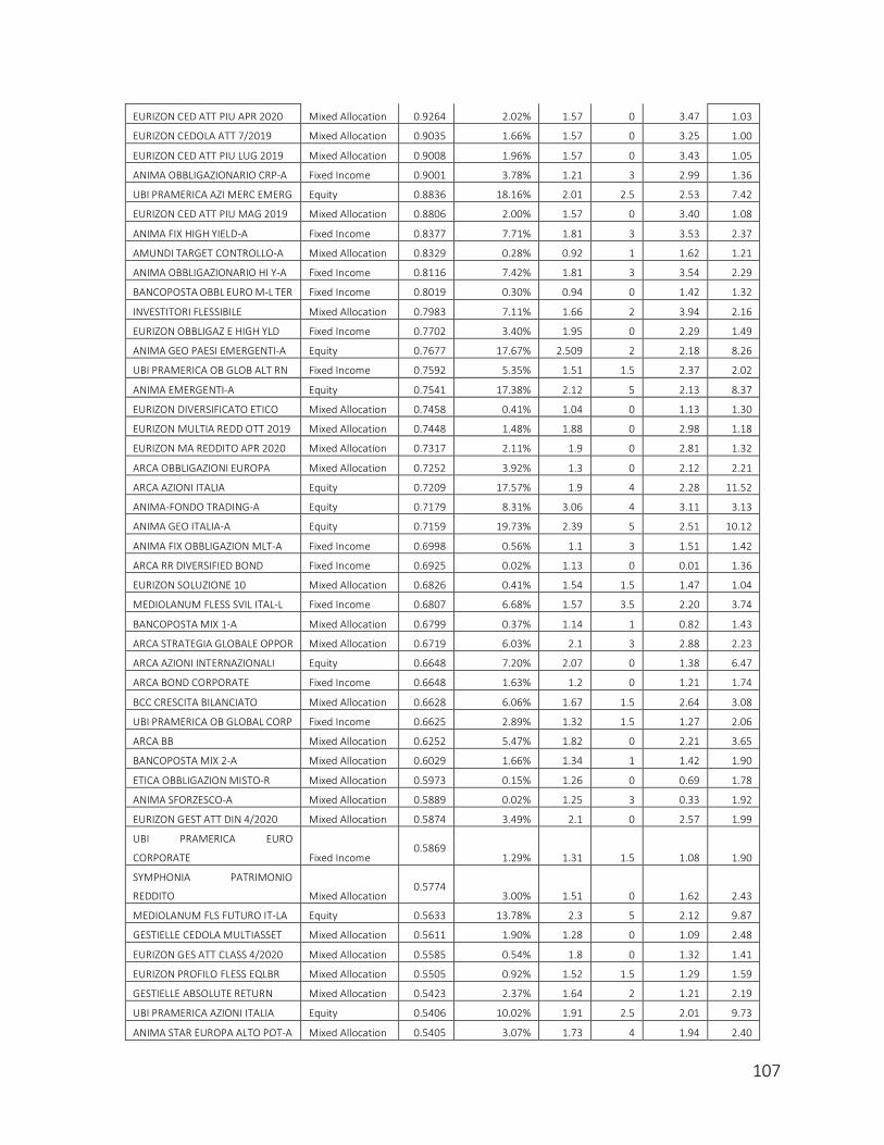
107

EURIZON CED ATT PIU APR 2020 Mixed Allocation 0.9264 2.02% 1.57 0 3.47 1.03

EURIZON CEDOLA ATT 7/2019 Mixed Allocation 0.9035 1.66% 1.57 0 3.25 1.00

EURIZON CED ATT PIU LUG 2019 Mixed Allocation 0.9008 1.96% 1.57 0 3.43 1.05

ANIMA OBBLIGAZIONARIO CRP-A Fixed Income 0.9001 3.78% 1.21 3 2.99 1.36

UBI PRAMERICA AZI MERC EMERG Equity 0.8836 18.16% 2.01 2.5 2.53 7.42

EURIZON CED ATT PIU MAG 2019 Mixed Allocation 0.8806 2.00% 1.57 0 3.40 1.08

ANIMA FIX HIGH YIELD-A Fixed Income 0.8377 7.71% 1.81 3 3.53 2.37

AMUNDI TARGET CONTROLLO-A Mixed Allocation 0.8329 0.28% 0.92 1 1.62 1.21

ANIMA OBBLIGAZIONARIO HI Y-A Fixed Income 0.8116 7.42% 1.81 3 3.54 2.29

BANCOPOSTA OBBL EURO M-L TER Fixed Income 0.8019 0.30% 0.94 0 1.42 1.32

INVESTITORI FLESSIBILE Mixed Allocation 0.7983 7.11% 1.66 2 3.94 2.16

EURIZON OBBLIGAZ E HIGH YLD Fixed Income 0.7702 3.40% 1.95 0 2.29 1.49

ANIMA GEO PAESI EMERGENTI-A Equity 0.7677 17.67% 2.509 2 2.18 8.26

UBI PRAMERICA OB GLOB ALT RN Fixed Income 0.7592 5.35% 1.51 1.5 2.37 2.02

ANIMA EMERGENTI-A Equity 0.7541 17.38% 2.12 5 2.13 8.37

EURIZON DIVERSIFICATO ETICO Mixed Allocation 0.7458 0.41% 1.04 0 1.13 1.30

EURIZON MULTIA REDD OTT 2019 Mixed Allocation 0.7448 1.48% 1.88 0 2.98 1.18

EURIZON MA REDDITO APR 2020 Mixed Allocation 0.7317 2.11% 1.9 0 2.81 1.32

ARCA OBBLIGAZIONI EUROPA Mixed Allocation 0.7252 3.92% 1.3 0 2.12 2.21

ARCA AZIONI ITALIA Equity 0.7209 17.57% 1.9 4 2.28 11.52

ANIMA-FONDO TRADING-A Equity 0.7179 8.31% 3.06 4 3.11 3.13

ANIMA GEO ITALIA-A Equity 0.7159 19.73% 2.39 5 2.51 10.12

ANIMA FIX OBBLIGAZION MLT-A Fixed Income 0.6998 0.56% 1.1 3 1.51 1.42

ARCA RR DIVERSIFIED BOND Fixed Income 0.6925 0.02% 1.13 0 0.01 1.36

EURIZON SOLUZIONE 10 Mixed Allocation 0.6826 0.41% 1.54 1.5 1.47 1.04

MEDIOLANUM FLESS SVIL ITAL-L Fixed Income 0.6807 6.68% 1.57 3.5 2.20 3.74

BANCOPOSTA MIX 1-A Mixed Allocation 0.6799 0.37% 1.14 1 0.82 1.43

ARCA STRATEGIA GLOBALE OPPOR Mixed Allocation 0.6719 6.03% 2.1 3 2.88 2.23

ARCA AZIONI INTERNAZIONALI Equity 0.6648 7.20% 2.07 0 1.38 6.47

ARCA BOND CORPORATE Fixed Income 0.6648 1.63% 1.2 0 1.21 1.74

BCC CRESCITA BILANCIATO Mixed Allocation 0.6628 6.06% 1.67 1.5 2.64 3.08

UBI PRAMERICA OB GLOBAL CORP Fixed Income 0.6625 2.89% 1.32 1.5 1.27 2.06

ARCA BB Mixed Allocation 0.6252 5.47% 1.82 0 2.21 3.65

BANCOPOSTA MIX 2-A Mixed Allocation 0.6029 1.66% 1.34 1 1.42 1.90

ETICA OBBLIGAZION MISTO-R Mixed Allocation 0.5973 0.15% 1.26 0 0.69 1.78

ANIMA SFORZESCO-A Mixed Allocation 0.5889 0.02% 1.25 3 0.33 1.92

EURIZON GEST ATT DIN 4/2020 Mixed Allocation 0.5874 3.49% 2.1 0 2.57 1.99

UBI PRAMERICA EURO

CORPORATE Fixed Income 0.5869

1.29% 1.31 1.5 1.08 1.90

SYMPHONIA PATRIMONIO

REDDITO Mixed Allocation 0.5774

3.00% 1.51 0 1.62 2.43

MEDIOLANUM FLS FUTURO IT-LA Equity 0.5633 13.78% 2.3 5 2.12 9.87

GESTIELLE CEDOLA MULTIASSET Mixed Allocation 0.5611 1.90% 1.28 0 1.09 2.48

EURIZON GES ATT CLASS 4/2020 Mixed Allocation 0.5585 0.54% 1.8 0 1.32 1.41

EURIZON PROFILO FLESS EQLBR Mixed Allocation 0.5505 0.92% 1.52 1.5 1.29 1.59

GESTIELLE ABSOLUTE RETURN Mixed Allocation 0.5423 2.37% 1.64 2 1.21 2.19

UBI PRAMERICA AZIONI ITALIA Equity 0.5406 10.02% 1.91 2.5 2.01 9.73

ANIMA STAR EUROPA ALTO POT-A Mixed Allocation 0.5405 3.07% 1.73 4 1.94 2.40

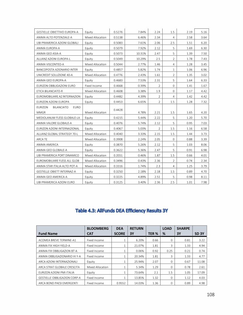
108

GESTIELLE OBIETTIVO EUROPA-A Equity 0.5276 7.84% 2.24 1.5 2.19 5.16

ANIMA ALTO POTENZIALE-A Mixed Allocation 0.5138 6.46% 2.34 4 2.58 3.64

UBI PRAMERICA AZIONI GLOBALI Equity 0.5083 7.61% 2.06 2.5 1.51 6.20

ANIMA EUROPA-A Equity 0.5079 7.92% 2.12 5 1.69 6.30

ANIMA GEO ASIA-A Equity 0.5073 10.31% 2.47 5 1.39 7.50

ALLIANZ AZIONI EUROPA-L Equity 0.5049 10.29% 2.5 2 1.78 7.43

ANIMA VISCONTEO-A Mixed Allocation 0.5044 2.77% 1.46 4 1.28 3.45

BANCOPOSTA AZIONARIO INTER Equity 0.4857 5.82% 1.74 1 1.06 6.96

UNICREDIT SOLUZIONE 40-A Mixed Allocation 0.4776 2.43% 1.61 2 1.35 3.02

ANIMA GEO EUROPA-A Equity 0.4683 7.53% 2.31 5 1.64 6.33

EURIZON OBBLIGAZIONI EURO Fixed Income 0.4668 0.39% 2 0 1.41 1.67

ETICA BILANCIATO-R Mixed Allocation 0.4608 3.38% 1.9 0 1.17 4.42

EUROMOBILIARE AZ INTERNAZION Equity 0.4482 4.39% 2 4 1.42 4.42

EURIZON AZIONI EUROPA Equity 0.4453 6.65% 2 1.5 1.28 7.32

EURIZON BILANCIATO EURO

MMGR Mixed Allocation 0.4428

4.78% 2.21 1.5 1.65 4.20

MEDIOLANUM FLESS GLOBALE-LA Equity 0.4215 5.44% 2.22 5 1.20 5.70

ANIMA VALORE GLOBALE-A Equity 0.4076 5.74% 2.12 5 0.95 7.03

EURIZON AZIONI INTERNAZIONAL Equity 0.4067 5.03% 2 1.5 1.16 6.58

ALLIANZ GLOBAL STRATEGY 70-L Mixed Allocation 0.4040 3.33% 2.15 1.5 1.44 3.73

ARCA TE Mixed Allocation 0.3908 2.24% 2.05 0 0.88 3.39

ANIMA AMERICA Equity 0.3870 5.26% 2.12 5 1.03 8.06

ANIMA GEO GLOBALE-A Equity 0.3622 5.36% 2.47 5 0.91 6.98

UBI PRAMERICA PORT DINAMICO Mixed Allocation 0.3551 0.46% 1.87 1.5 0.66 4.01

EUROMOBILIARE FLESS ALL GLOB Mixed Allocation 0.3496 0.43% 2.36 2 0.74 2.34

ANIMA STAR ITALIA ALTO POT-A Mixed Allocation 0.3316 1.74% 2.3 4 1.25 3.79

GESTIELLE OBIETT INTERNAZ-A Equity 0.3250 2.18% 2.18 1.5 0.89 4.70

ANIMA GEO AMERICA-A Equity 0.3225 4.89% 2.51 5 0.98 8.11

UBI PRAMERICA AZIONI EURO Equity 0.3125 3.40% 2.36 2.5 1.01 7.98

Table 4.3: AllFunds DEA Efficiency Results 3Y

Fund Name BLOOMBERG CAT

DEA SCORE

RETURN 3Y TER %

LOAD %

SHARPE 3Y SD 3Y

ACOMEA BREVE TERMINE-A1 Fixed Income 1 6.20% 0.66 0 0.81 3.22

ANIMA FIX HIGH YIELD-A Fixed Income 1 21.07% 1.81 3 1.33 4.94

ANIMA FIX OBBLIGAZION BT-A Fixed Income 1 0.06% 0.92 0.25 0.21 0.74

ANIMA OBBLIGAZIONARIO HI Y-A Fixed Income 1 20.34% 1.81 3 1.33 4.77

ARCA AZIONI INTERNAZIONALI Equity 1 25.94% 2.07 0 0.67 11.08

ARCA STRAT GLOBALE CRESCITA Mixed Allocation 1 5.34% 1.29 0 0.78 2.61

EURIZON AZIONI PMI ITALIA Equity 1 73.64% 2.1 1.5 1.05 17.09

GESTIELLE OBBLIGAZION CORP-A Fixed Income 1 13.85% 1.32 0 1.12 4.03

ARCA BOND PAESI EMERGENTI Fixed Income 0.9552 14.03% 1.36 0 0.89 4.98

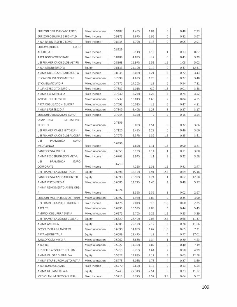
109

EURIZON DIVERSIFICATO ETICO Mixed Allocation 0.9487 4.40% 1.04 0 0.48 2.93

EURIZON OBBLIGAZ E HIGH YLD Fixed Income 0.9173 9.87% 1.95 0 0.82 3.67

ARCA RR DIVERSIFIED BOND Fixed Income 0.8735 1.79% 1.13 0 0.05 2.91

EUROMOBILIARE EURO

AGGREGATE Fixed Income 0.8629

0.11% 1.13 1 0.13 0.87

ARCA BOND CORPORATE Fixed Income 0.8488 4.83% 1.2 0 0.41 3.29

UBI PRAMERICA OB GLOB ALT RN Fixed Income 0.8368 15.97% 1.51 1.5 1.08 5.02

ARCA AZIONI EUROPA Equity 0.8133 21.10% 2.12 0 0.47 12.41

ANIMA OBBLIGAZIONARIO CRP-A Fixed Income 0.8035 8.06% 1.21 3 0.72 3.43

ETICA OBBLIGAZION MISTO-R Mixed Allocation 0.7998 4.63% 1.26 0 0.27 3.48

ETICA BILANCIATO-R Mixed Allocation 0.7975 17.20% 1.9 0 0.54 7.81

ALLIANZ REDDITO EURO-L Fixed Income 0.7887 1.01% 0.9 1.5 -0.01 3.48

ANIMA FIX IMPRESE-A Fixed Income 0.7830 8.23% 1.26 3 0.74 3.52

INVESTITORI FLESSIBILE Mixed Allocation 0.7737 13.81% 1.66 2 0.84 4.75

ARCA OBBLIGAZIONI EUROPA Mixed Allocation 0.7593 10.01% 1.3 0 0.47 4.81

ANIMA SFORZESCO-A Mixed Allocation 0.7549 6.40% 1.25 3 0.37 3.17

EURIZON OBBLIGAZIONI EURO Fixed Income 0.7244 3.36% 2 0 0.15 3.54

SYMPHONIA PATRIMONIO

REDDITO Mixed Allocation 0.7159

5.08% 1.51 0 0.32 3.86

UBI PRAMERICA GLB HI YD EU H Fixed Income 0.7126 1.43% 1.29 0 0.46 3.60

UBI PRAMERICA OB GLOBAL CORP Fixed Income 0.7079 6.37% 1.32 1.5 0.35 3.41

UBI PRAMERICA EURO

MED/LUNGO Fixed Income 0.6896

1.89% 1.11 1.5 0.00 3.21

BANCOPOSTA MIX 1-A Mixed Allocation 0.6859 3.13% 1.14 1 0.11 3.00

ANIMA FIX OBBLIGAZION MLT-A Fixed Income 0.6762 3.94% 1.1 3 0.22 3.58

UBI PRAMERICA EURO

CORPORATE Fixed Income 0.6719

4.22% 1.31 1.5 0.41 2.97

UBI PRAMERICA AZIONI ITALIA Equity 0.6696 35.19% 1.91 2.5 0.69 15.16

BANCOPOSTA AZIONARIO INTER Equity 0.6590 28.99% 1.74 1 0.62 12.58

ANIMA VISCONTEO-A Mixed Allocation 0.6585 11.77% 1.46 4 0.49 5.77

ANIMA RENDIMENTO ASSOL OBB-

A Fixed Income 0.6524

3.36% 1.36 3 0.02 2.67

EURIZON MULTIA REDD OTT 2019 Mixed Allocation 0.6492 1.96% 1.88 0 0.35 3.90

UBI PRAMERICA PORT PRUDENTE Fixed Income 0.6476 2.04% 1.3 1.5 0.00 2.35

ARCA TE Mixed Allocation 0.6395 10.58% 2.05 0 0.44 5.45

AMUNDI OBBL PIU A DIST-A Mixed Allocation 0.6375 2.70% 1.22 1.2 0.23 3.29

UBI PRAMERICA AZIONI GLOBALI Equity 0.6329 28.40% 2.06 2.5 0.68 11.47

ANIMA AMERICA Equity 0.6305 29.12% 2.12 5 0.78 11.66

BCC CRESCITA BILANCIATO Mixed Allocation 0.6090 14.80% 1.67 1.5 0.65 7.31

ARCA AZIONI ITALIA Equity 0.6089 29.47% 1.9 4 0.57 17.01

BANCOPOSTA MIX 2-A Mixed Allocation 0.5962 5.88% 1.34 1 0.20 4.53

ARCA BB Mixed Allocation 0.5927 11.35% 1.82 0 0.40 7.19

GESTIELLE ABSOLUTE RETURN Mixed Allocation 0.5915 8.76% 1.64 2 0.50 4.99

ANIMA VALORE GLOBALE-A Equity 0.5827 27.88% 2.12 5 0.63 12.58

ANIMA STAR EUROPA ALTO POT-A Mixed Allocation 0.5773 6.06% 1.73 4 0.27 3.69

ARCA BOND GLOBALE Fixed Income 0.5770 5.60% 1.16 0 -0.13 5.54

ANIMA GEO AMERICA-A Equity 0.5743 27.34% 2.51 5 0.73 11.72

MEDIOLANUM FLESS SVIL ITAL-L Fixed Income 0.5713 8.77% 1.57 3.5 0.64 5.57

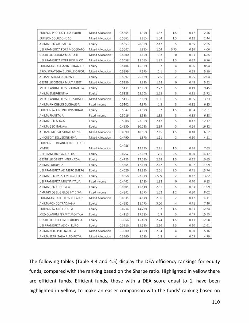
110

EURIZON PROFILO FLESS EQLBR Mixed Allocation 0.5665 1.99% 1.52 1.5 0.17 2.56

EURIZON SOLUZIONE 10 Mixed Allocation 0.5662 1.86% 1.54 1.5 0.12 2.44

ANIMA GEO GLOBALE-A Equity 0.5653 28.96% 2.47 5 0.65 12.65

UBI PRAMERICA PORT MODERATO Mixed Allocation 0.5647 5.83% 1.64 0.75 0.16 4.06

GESTIELLE CEDOLA MULTIA II Mixed Allocation 0.5500 3.80% 1.2 0 0.31 6.85

UBI PRAMERICA PORT DINAMICO Mixed Allocation 0.5458 12.05% 1.87 1.5 0.37 6.76

EUROMOBILIARE AZ INTERNAZION Equity 0.5404 16.93% 2 4 0.56 8.94

ARCA STRATEGIA GLOBALE OPPOR Mixed Allocation 0.5399 9.57% 2.1 3 0.68 5.19

ALLIANZ AZIONI EUROPA-L Equity 0.5397 26.02% 2.5 2 0.55 12.04

GESTIELLE CEDOLA MULTIASSET Mixed Allocation 0.5339 2.63% 1.28 0 0.48 5.92

MEDIOLANUM FLESS GLOBALE-LA Equity 0.5131 17.66% 2.22 5 0.49 9.45

ANIMA EMERGENTI-A Equity 0.5128 25.10% 2.12 5 0.52 13.72

MEDIOLANUM FLESSIBLE STRAT-L Mixed Allocation 0.5113 2.88% 1.56 3.5 0.35 3.73

ANIMA FIX OBBLIG GLOBALE-A Fixed Income 0.5102 4.37% 1.3 3 -0.32 6.25

EURIZON AZIONI INTERNAZIONAL Equity 0.5047 21.57% 2 1.5 0.54 12.51

ANIMA PIANETA-A Fixed Income 0.5016 3.68% 1.32 3 -0.33 6.38

ANIMA GEO ASIA-A Equity 0.5008 23.36% 2.47 5 0.47 12.17

ANIMA GEO ITALIA-A Equity 0.4950 30.03% 2.39 5 0.56 16.32

ALLIANZ GLOBAL STRATEGY 70-L Mixed Allocation 0.4890 10.56% 2.15 1.5 0.48 6.52

UNICREDIT SOLUZIONE 40-A Mixed Allocation 0.4790 1.87% 1.61 2 0.10 4.51

EURIZON BILANCIATO EURO

MMGR Mixed Allocation 0.4786

12.33% 2.21 1.5 0.36 7.63

UBI PRAMERICA AZIONI USA Equity 0.4752 22.02% 2.1 2.5 0.50 14.17

GESTIELLE OBIETT INTERNAZ-A Equity 0.4725 17.09% 2.18 1.5 0.52 10.65

ANIMA EUROPA-A Equity 0.4664 17.13% 2.12 5 0.37 11.09

UBI PRAMERICA AZI MERC EMERG Equity 0.4626 18.83% 2.01 2.5 0.41 13.74

ANIMA GEO PAESI EMERGENTI-A Equity 0.4558 23.04% 2.509 2 0.47 13.82

UBI PRAMERICA MULTIA ITALIA Fixed Income 0.4442 2.78% 1.98 0 0.70 6.13

ANIMA GEO EUROPA-A Equity 0.4405 16.41% 2.31 5 0.34 11.09

AMUNDI OBBLIG GLOB HY DIS-A Fixed Income 0.4342 2.27% 1.52 1.2 0.30 8.02

EUROMOBILIARE FLESS ALL GLOB Mixed Allocation 0.4335 4.84% 2.36 2 0.17 4.11

ANIMA-FONDO TRADING-A Equity 0.4285 11.77% 3.06 4 0.71 7.40

EURIZON AZIONI EUROPA Equity 0.4216 14.78% 2 1.5 0.31 12.74

MEDIOLANUM FLS FUTURO IT-LA Equity 0.4115 19.62% 2.3 5 0.43 15.55

GESTIELLE OBIETTIVO EUROPA-A Equity 0.3966 15.46% 2.24 1.5 0.41 12.68

UBI PRAMERICA AZIONI EURO Equity 0.3916 15.53% 2.36 2.5 0.30 12.61

ANIMA ALTO POTENZIALE-A Mixed Allocation 0.3800 4.19% 2.34 4 0.30 5.16

ANIMA STAR ITALIA ALTO POT-A Mixed Allocation 0.3560 2.21% 2.3 4 0.03 4.79

The following tables (Table 4.4 and 4.5) display the DEA efficiency rankings for equity

funds, compared with the ranking based on the Sharpe ratio. Highlighted in yellow there

are efficient funds. Efficient funds, those with a DEA score equal to 1, have been

highlighted in yellow, to make an easier comparison with the funds’ ranking based on

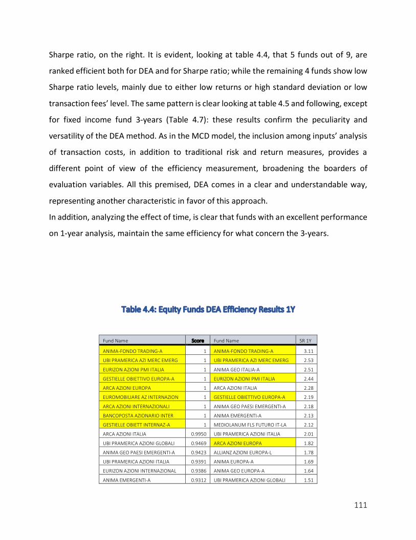
111

Sharpe ratio, on the right. It is evident, looking at table 4.4, that 5 funds out of 9, are

ranked efficient both for DEA and for Sharpe ratio; while the remaining 4 funds show low

Sharpe ratio levels, mainly due to either low returns or high standard deviation or low

transaction fees’ level. The same pattern is clear looking at table 4.5 and following, except

for fixed income fund 3-years (Table 4.7): these results confirm the peculiarity and

versatility of the DEA method. As in the MCD model, the inclusion among inputs’ analysis

of transaction costs, in addition to traditional risk and return measures, provides a

different point of view of the efficiency measurement, broadening the boarders of

evaluation variables. All this premised, DEA comes in a clear and understandable way,

representing another characteristic in favor of this approach.

In addition, analyzing the effect of time, is clear that funds with an excellent performance

on 1-year analysis, maintain the same efficiency for what concern the 3-years.

Table 4.4: Equity Funds DEA Efficiency Results 1Y

Fund Name Score Fund Name SR 1Y

ANIMA-FONDO TRADING-A 1 ANIMA-FONDO TRADING-A 3.11

UBI PRAMERICA AZI MERC EMERG 1 UBI PRAMERICA AZI MERC EMERG 2.53

EURIZON AZIONI PMI ITALIA 1 ANIMA GEO ITALIA-A 2.51

GESTIELLE OBIETTIVO EUROPA-A 1 EURIZON AZIONI PMI ITALIA 2.44

ARCA AZIONI EUROPA 1 ARCA AZIONI ITALIA 2.28

EUROMOBILIARE AZ INTERNAZION 1 GESTIELLE OBIETTIVO EUROPA-A 2.19

ARCA AZIONI INTERNAZIONALI 1 ANIMA GEO PAESI EMERGENTI-A 2.18

BANCOPOSTA AZIONARIO INTER 1 ANIMA EMERGENTI-A 2.13

GESTIELLE OBIETT INTERNAZ-A 1 MEDIOLANUM FLS FUTURO IT-LA 2.12

ARCA AZIONI ITALIA 0.9950 UBI PRAMERICA AZIONI ITALIA 2.01

UBI PRAMERICA AZIONI GLOBALI 0.9469 ARCA AZIONI EUROPA 1.82

ANIMA GEO PAESI EMERGENTI-A 0.9423 ALLIANZ AZIONI EUROPA-L 1.78

UBI PRAMERICA AZIONI ITALIA 0.9391 ANIMA EUROPA-A 1.69

EURIZON AZIONI INTERNAZIONAL 0.9386 ANIMA GEO EUROPA-A 1.64

ANIMA EMERGENTI-A 0.9312 UBI PRAMERICA AZIONI GLOBALI 1.51

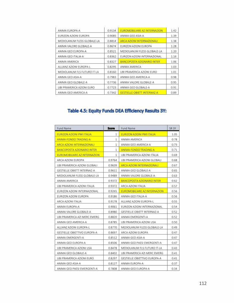
112

ANIMA EUROPA-A 0.9134 EUROMOBILIARE AZ INTERNAZION 1.42

EURIZON AZIONI EUROPA 0.9085 ANIMA GEO ASIA-A 1.39

MEDIOLANUM FLESS GLOBALE-LA 0.8814 ARCA AZIONI INTERNAZIONALI 1.38

ANIMA VALORE GLOBALE-A 0.8674 EURIZON AZIONI EUROPA 1.28

ANIMA GEO EUROPA-A 0.8521 MEDIOLANUM FLESS GLOBALE-LA 1.20

ANIMA GEO ITALIA-A 0.8362 EURIZON AZIONI INTERNAZIONAL 1.16

ANIMA AMERICA 0.8327 BANCOPOSTA AZIONARIO INTER 1.06

ALLIANZ AZIONI EUROPA-L 0.8295 ANIMA AMERICA 1.03

MEDIOLANUM FLS FUTURO IT-LA 0.8160 UBI PRAMERICA AZIONI EURO 1.01

ANIMA GEO ASIA-A 0.7983 ANIMA GEO AMERICA-A 0.98

ANIMA GEO GLOBALE-A 0.7736 ANIMA VALORE GLOBALE-A 0.95

UBI PRAMERICA AZIONI EURO 0.7723 ANIMA GEO GLOBALE-A 0.91

ANIMA GEO AMERICA-A 0.7342 GESTIELLE OBIETT INTERNAZ-A 0.89

Table 4.5: Equity Funds DEA Efficiency Results 3Y:

Fund Name Score Fund Name SR 3Y

EURIZON AZIONI PMI ITALIA 1 EURIZON AZIONI PMI ITALIA 1.05

ANIMA-FONDO TRADING-A 1 ANIMA AMERICA 0.78

ARCA AZIONI INTERNAZIONALI 1 ANIMA GEO AMERICA-A 0.73

BANCOPOSTA AZIONARIO INTER 1 ANIMA-FONDO TRADING-A 0.71

EUROMOBILIARE AZ INTERNAZION 1 UBI PRAMERICA AZIONI ITALIA 0.69

ARCA AZIONI EUROPA 0.9764 UBI PRAMERICA AZIONI GLOBALI 0.68

UBI PRAMERICA AZIONI GLOBALI 0.9639 ARCA AZIONI INTERNAZIONALI 0.67

GESTIELLE OBIETT INTERNAZ-A 0.9611 ANIMA GEO GLOBALE-A 0.65

MEDIOLANUM FLESS GLOBALE-LA 0.9489 ANIMA VALORE GLOBALE-A 0.63

ANIMA AMERICA 0.9372 BANCOPOSTA AZIONARIO INTER 0.62

UBI PRAMERICA AZIONI ITALIA 0.9372 ARCA AZIONI ITALIA 0.57

EURIZON AZIONI INTERNAZIONAL 0.9265 EUROMOBILIARE AZ INTERNAZION 0.56

EURIZON AZIONI EUROPA 0.9186 ANIMA GEO ITALIA-A 0.56

ARCA AZIONI ITALIA 0.9178 ALLIANZ AZIONI EUROPA-L 0.55

ANIMA EUROPA-A 0.9061 EURIZON AZIONI INTERNAZIONAL 0.54

ANIMA VALORE GLOBALE-A 0.8980 GESTIELLE OBIETT INTERNAZ-A 0.52

UBI PRAMERICA AZI MERC EMERG 0.8820 ANIMA EMERGENTI-A 0.52

ANIMA GEO AMERICA-A 0.8785 UBI PRAMERICA AZIONI USA 0.50

ALLIANZ AZIONI EUROPA-L 0.8770 MEDIOLANUM FLESS GLOBALE-LA 0.49

GESTIELLE OBIETTIVO EUROPA-A 0.8697 ARCA AZIONI EUROPA 0.47

ANIMA EMERGENTI-A 0.8512 ANIMA GEO ASIA-A 0.47

ANIMA GEO EUROPA-A 0.8506 ANIMA GEO PAESI EMERGENTI-A 0.47

UBI PRAMERICA AZIONI USA 0.8478 MEDIOLANUM FLS FUTURO IT-LA 0.43

ANIMA GEO GLOBALE-A 0.8402 UBI PRAMERICA AZI MERC EMERG 0.41

UBI PRAMERICA AZIONI EURO 0.8297 GESTIELLE OBIETTIVO EUROPA-A 0.41

ANIMA GEO ASIA-A 0.8127 ANIMA EUROPA-A 0.37

ANIMA GEO PAESI EMERGENTI-A 0.7808 ANIMA GEO EUROPA-A 0.34

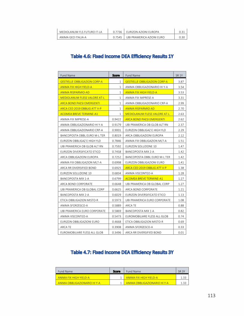
113

MEDIOLANUM FLS FUTURO IT-LA 0.7736 EURIZON AZIONI EUROPA 0.31

ANIMA GEO ITALIA-A 0.7545 UBI PRAMERICA AZIONI EURO 0.30

Table 4.6: Fixed Income DEA Efficiency Results 1Y

Fund Name Score Fund Name SR 1Y

GESTIELLE OBBLIGAZION CORP-A 1 GESTIELLE OBBLIGAZION CORP-A 3.87

ANIMA FIX HIGH YIELD-A 1 ANIMA OBBLIGAZIONARIO HI Y-A 3.54

ANIMA RISPARMIO-AD 1 ANIMA FIX HIGH YIELD-A 3.53

MEDIOLANUM FLESS VALORE AT-L 1 ANIMA FIX IMPRESE-A 3.31

ARCA BOND PAESI EMERGENTI 1 ANIMA OBBLIGAZIONARIO CRP-A 2.99

ARCA CED 2019 OBBLIG ATT V-P 1 ANIMA RISPARMIO-AD 2.70

ACOMEA BREVE TERMINE-A1 1 MEDIOLANUM FLESS VALORE AT-L 2.63

ANIMA FIX IMPRESE-A 0.9422 ARCA BOND PAESI EMERGENTI 2.62

ANIMA OBBLIGAZIONARIO HI Y-A 0.9179 UBI PRAMERICA OB GLOB ALT RN 2.37

ANIMA OBBLIGAZIONARIO CRP-A 0.9001 EURIZON OBBLIGAZ E HIGH YLD 2.29

BANCOPOSTA OBBL EURO M-L TER 0.8019 ARCA OBBLIGAZIONI EUROPA 2.12

EURIZON OBBLIGAZ E HIGH YLD 0.7846 ANIMA FIX OBBLIGAZION MLT-A 1.51

UBI PRAMERICA OB GLOB ALT RN 0.7592 EURIZON SOLUZIONE 10 1.47

EURIZON DIVERSIFICATO ETICO 0.7458 BANCOPOSTA MIX 2-A 1.42

ARCA OBBLIGAZIONI EUROPA 0.7252 BANCOPOSTA OBBL EURO M-L TER 1.42

ANIMA FIX OBBLIGAZION MLT-A 0.6998 EURIZON OBBLIGAZIONI EURO 1.41

ARCA RR DIVERSIFIED BOND 0.6925 ARCA CED 2019 OBBLIG ATT V-P 1.38

EURIZON SOLUZIONE 10 0.6834 ANIMA VISCONTEO-A 1.28

BANCOPOSTA MIX 1-A 0.6799 ACOMEA BREVE TERMINE-A1 1.27

ARCA BOND CORPORATE 0.6648 UBI PRAMERICA OB GLOBAL CORP 1.27

UBI PRAMERICA OB GLOBAL CORP 0.6625 ARCA BOND CORPORATE 1.21

BANCOPOSTA MIX 2-A 0.6029 EURIZON DIVERSIFICATO ETICO 1.13

ETICA OBBLIGAZION MISTO-R 0.5973 UBI PRAMERICA EURO CORPORATE 1.08

ANIMA SFORZESCO-A 0.5889 ARCA TE 0.88

UBI PRAMERICA EURO CORPORATE 0.5869 BANCOPOSTA MIX 1-A 0.82

ANIMA VISCONTEO-A 0.5473 EUROMOBILIARE FLESS ALL GLOB 0.74

EURIZON OBBLIGAZIONI EURO 0.4668 ETICA OBBLIGAZION MISTO-R 0.69

ARCA TE 0.3908 ANIMA SFORZESCO-A 0.33

EUROMOBILIARE FLESS ALL GLOB 0.3496 ARCA RR DIVERSIFIED BOND 0.01

Table 4.7: Fixed Income DEA Efficiency Results 3Y

Fund Name Score Fund Name SR 3Y

ANIMA FIX HIGH YIELD-A 1 ANIMA FIX HIGH YIELD-A 1.33

ANIMA OBBLIGAZIONARIO HI Y-A 1 ANIMA OBBLIGAZIONARIO HI Y-A 1.33

114

GESTIELLE OBBLIGAZION CORP-A 1 GESTIELLE OBBLIGAZION CORP-A 1.12

ARCA BOND PAESI EMERGENTI 1 UBI PRAMERICA OB GLOB ALT RN 1.08

ACOMEA BREVE TERMINE-A1 1 ARCA BOND PAESI EMERGENTI 0.89

ANIMA FIX OBBLIGAZION BT-A 1 EURIZON OBBLIGAZ E HIGH YLD 0.82

BANCOPOSTA OBBL EURO M-L TER 1 ACOMEA BREVE TERMINE-A1 0.81

EURIZON DIVERSIFICATO ETICO 0.9939 ANIMA FIX IMPRESE-A 0.74

EURIZON OBBLIGAZ E HIGH YLD 0.9698 ANIMA OBBLIGAZIONARIO CRP-A 0.72

UBI PRAMERICA OB GLOB ALT RN 0.9532 UBI PRAMERICA MULTIA ITALIA 0.70

ARCA BOND CORPORATE 0.9002 ANIMA VISCONTEO-A 0.49

ARCA RR DIVERSIFIED BOND 0.8944 EURIZON DIVERSIFICATO ETICO 0.48

EUROMOBILIARE EURO AGGREGATE 0.8629 ARCA OBBLIGAZIONI EUROPA 0.47

ANIMA OBBLIGAZIONARIO CRP-A 0.8469 UBI PRAMERICA GLB HI YD EU H 0.46

ETICA OBBLIGAZION MISTO-R 0.8442 ARCA TE 0.44

ANIMA FIX IMPRESE-A 0.8272 ARCA BOND CORPORATE 0.41

ALLIANZ REDDITO EURO-L 0.7887 UBI PRAMERICA EURO CORPORATE 0.41

ANIMA SFORZESCO-A 0.7881 ANIMA SFORZESCO-A 0.37

EURIZON OBBLIGAZIONI EURO 0.7877 UBI PRAMERICA OB GLOBAL CORP 0.35

ARCA OBBLIGAZIONI EUROPA 0.7605 AMUNDI OBBLIG GLOB HY DIS-A 0.30

ANIMA VISCONTEO-A 0.7474 ETICA OBBLIGAZION MISTO-R 0.27

UBI PRAMERICA OB GLOBAL CORP 0.7380 AMUNDI OBBL PIU A DIST-A 0.23

UBI PRAMERICA GLB HI YD EU H 0.7129 ANIMA FIX OBBLIGAZION MLT-A 0.22

UBI PRAMERICA EURO MED/LUNGO 0.6896 ANIMA FIX OBBLIGAZION BT-A 0.21

UBI PRAMERICA EURO CORPORATE 0.6876 BANCOPOSTA MIX 2-A 0.20

BANCOPOSTA MIX 1-A 0.6859 EUROMOBILIARE FLESS ALL GLOB 0.17

ANIMA FIX OBBLIGAZION MLT-A 0.6762 UBI PRAMERICA PORT MODERATO 0.16

ARCA TE 0.6685 EURIZON OBBLIGAZIONI EURO 0.15

ANIMA RENDIMENTO ASSOL OBB-A 0.6651 EUROMOBILIARE EURO AGGREGATE 0.13

UBI PRAMERICA PORT PRUDENTE 0.6483 EURIZON SOLUZIONE 10 0.12

AMUNDI OBBL PIU A DIST-A 0.6375 BANCOPOSTA MIX 1-A 0.11

BANCOPOSTA MIX 2-A 0.6076 BANCOPOSTA OBBL EURO M-L TER 0.07

UBI PRAMERICA PORT MODERATO 0.5878 ARCA RR DIVERSIFIED BOND 0.05

ARCA BOND GLOBALE 0.5770 ANIMA RENDIMENTO ASSOL OBB-A 0.02

EURIZON SOLUZIONE 10 0.5694 UBI PRAMERICA EURO MED/LUNGO 0.00

ANIMA FIX OBBLIG GLOBALE-A 0.5102 UBI PRAMERICA PORT PRUDENTE 0.00

ANIMA PIANETA-A 0.5016 ALLIANZ REDDITO EURO-L -0.01

EUROMOBILIARE FLESS ALL GLOB 0.4493 ARCA BOND GLOBALE -0.13

UBI PRAMERICA MULTIA ITALIA 0.4475 ANIMA FIX OBBLIG GLOBALE-A -0.32

AMUNDI OBBLIG GLOB HY DIS-A 0.4342 ANIMA PIANETA-A -0.33

Table 4.8: Mixed Allocation DEA Efficiency Results 1Y

Fund Name Score Fund Name SR 1Y

INVESTITORI FLESSIBILE 1 INVESTITORI FLESSIBILE 3.94

EURIZON CEDOLA ATT APR 2020 1 EURIZON CED ATT PIU OTT 2019 3.52

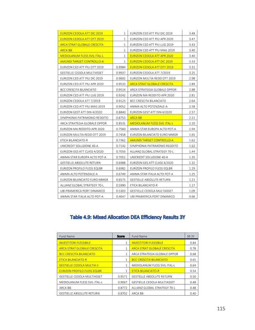
115

EURIZON CEDOLA ATT DIC 2019 1 EURIZON CED ATT PIU DIC 2019 3.48

EURIZON CEDOLA ATT OTT 2019 1 EURIZON CED ATT PIU APR 2020 3.47

ARCA STRAT GLOBALE CRESCITA 1 EURIZON CED ATT PIU LUG 2019 3.43

ARCA BB 1 EURIZON CED ATT PIU MAG 2019 3.40

MEDIOLANUM FLESS SVIL ITAL-L 1 EURIZON CEDOLA ATT APR 2020 3.40

AMUNDI TARGET CONTROLLO-A 1 EURIZON CEDOLA ATT DIC 2019 3.33

EURIZON CED ATT PIU OTT 2019 0.9984 EURIZON CEDOLA ATT OTT 2019 3.31

GESTIELLE CEDOLA MULTIASSET 0.9937 EURIZON CEDOLA ATT 7/2019 3.25

EURIZON CED ATT PIU DIC 2019 0.9692 EURIZON MULTIA REDD OTT 2019 2.98

EURIZON CED ATT PIU APR 2020 0.9533 ARCA STRAT GLOBALE CRESCITA 2.89

BCC CRESCITA BILANCIATO 0.9514 ARCA STRATEGIA GLOBALE OPPOR 2.88

EURIZON CED ATT PIU LUG 2019 0.9242 EURIZON MA REDDITO APR 2020 2.81

EURIZON CEDOLA ATT 7/2019 0.9123 BCC CRESCITA BILANCIATO 2.64

EURIZON CED ATT PIU MAG 2019 0.9052 ANIMA ALTO POTENZIALE-A 2.58

EURIZON GEST ATT DIN 4/2020 0.8840 EURIZON GEST ATT DIN 4/2020 2.57

SYMPHONIA PATRIMONIO REDDITO 0.8753 ARCA BB 2.21

ARCA STRATEGIA GLOBALE OPPOR 0.8531 MEDIOLANUM FLESS SVIL ITAL-L 2.20

EURIZON MA REDDITO APR 2020 0.7560 ANIMA STAR EUROPA ALTO POT-A 1.94

EURIZON MULTIA REDD OTT 2019 0.7458 EURIZON BILANCIATO EURO MMGR 1.65

ETICA BILANCIATO-R 0.7362 AMUNDI TARGET CONTROLLO-A 1.62

UNICREDIT SOLUZIONE 40-A 0.7142 SYMPHONIA PATRIMONIO REDDITO 1.62

EURIZON GES ATT CLASS 4/2020 0.7056 ALLIANZ GLOBAL STRATEGY 70-L 1.44

ANIMA STAR EUROPA ALTO POT-A 0.7052 UNICREDIT SOLUZIONE 40-A 1.35

GESTIELLE ABSOLUTE RETURN 0.6988 EURIZON GES ATT CLASS 4/2020 1.32

EURIZON PROFILO FLESS EQLBR 0.6982 EURIZON PROFILO FLESS EQLBR 1.29

ANIMA ALTO POTENZIALE-A 0.6749 ANIMA STAR ITALIA ALTO POT-A 1.25

EURIZON BILANCIATO EURO MMGR 0.6575 GESTIELLE ABSOLUTE RETURN 1.21

ALLIANZ GLOBAL STRATEGY 70-L 0.5990 ETICA BILANCIATO-R 1.17

UBI PRAMERICA PORT DINAMICO 0.5303 GESTIELLE CEDOLA MULTIASSET 1.09

ANIMA STAR ITALIA ALTO POT-A 0.4647 UBI PRAMERICA PORT DINAMICO 0.66

Table 4.9: Mixed Allocation DEA Efficiency Results 3Y

Fund Name Score Fund Name SR 3Y

INVESTITORI FLESSIBILE 1 INVESTITORI FLESSIBILE 0.84

ARCA STRAT GLOBALE CRESCITA 1 ARCA STRAT GLOBALE CRESCITA 0.78

BCC CRESCITA BILANCIATO 1 ARCA STRATEGIA GLOBALE OPPOR 0.68

ETICA BILANCIATO-R 1 BCC CRESCITA BILANCIATO 0.65

GESTIELLE CEDOLA MULTIA II 1 MEDIOLANUM FLESS SVIL ITAL-L 0.64

EURIZON PROFILO FLESS EQLBR 1 ETICA BILANCIATO-R 0.54

GESTIELLE CEDOLA MULTIASSET 0.9571 GESTIELLE ABSOLUTE RETURN 0.50

MEDIOLANUM FLESS SVIL ITAL-L 0.9067 GESTIELLE CEDOLA MULTIASSET 0.48

ARCA BB 0.8772 ALLIANZ GLOBAL STRATEGY 70-L 0.48

GESTIELLE ABSOLUTE RETURN 0.8702 ARCA BB 0.40

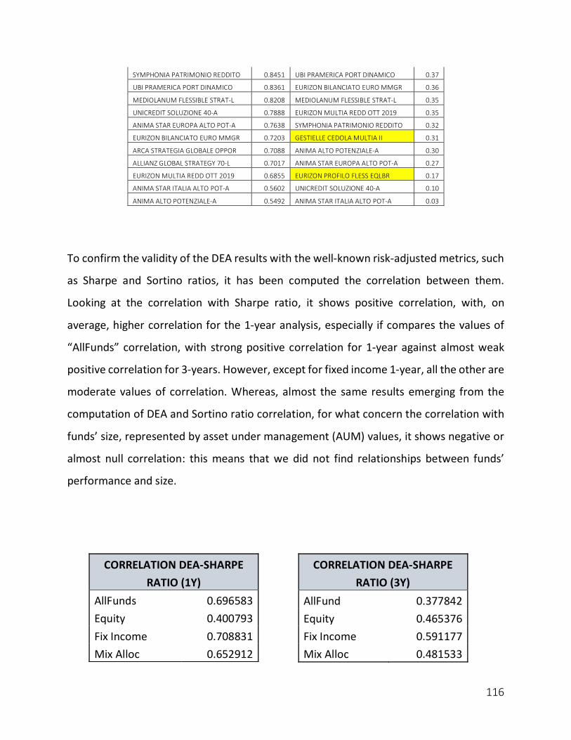
116

SYMPHONIA PATRIMONIO REDDITO 0.8451 UBI PRAMERICA PORT DINAMICO 0.37

UBI PRAMERICA PORT DINAMICO 0.8361 EURIZON BILANCIATO EURO MMGR 0.36

MEDIOLANUM FLESSIBLE STRAT-L 0.8208 MEDIOLANUM FLESSIBLE STRAT-L 0.35

UNICREDIT SOLUZIONE 40-A 0.7888 EURIZON MULTIA REDD OTT 2019 0.35

ANIMA STAR EUROPA ALTO POT-A 0.7638 SYMPHONIA PATRIMONIO REDDITO 0.32

EURIZON BILANCIATO EURO MMGR 0.7203 GESTIELLE CEDOLA MULTIA II 0.31

ARCA STRATEGIA GLOBALE OPPOR 0.7088 ANIMA ALTO POTENZIALE-A 0.30

ALLIANZ GLOBAL STRATEGY 70-L 0.7017 ANIMA STAR EUROPA ALTO POT-A 0.27

EURIZON MULTIA REDD OTT 2019 0.6855 EURIZON PROFILO FLESS EQLBR 0.17

ANIMA STAR ITALIA ALTO POT-A 0.5602 UNICREDIT SOLUZIONE 40-A 0.10

ANIMA ALTO POTENZIALE-A 0.5492 ANIMA STAR ITALIA ALTO POT-A 0.03

To confirm the validity of the DEA results with the well-known risk-adjusted metrics, such

as Sharpe and Sortino ratios, it has been computed the correlation between them.

Looking at the correlation with Sharpe ratio, it shows positive correlation, with, on

average, higher correlation for the 1-year analysis, especially if compares the values of

“AllFunds” correlation, with strong positive correlation for 1-year against almost weak

positive correlation for 3-years. However, except for fixed income 1-year, all the other are

moderate values of correlation. Whereas, almost the same results emerging from the

computation of DEA and Sortino ratio correlation, for what concern the correlation with

funds’ size, represented by asset under management (AUM) values, it shows negative or

almost null correlation: this means that we did not find relationships between funds’

performance and size.

CORRELATION DEA-SHARPE RATIO (3Y)

AllFund 0.377842 Equity 0.465376 Fix Income 0.591177 Mix Alloc 0.481533

CORRELATION DEA-SHARPE RATIO (1Y)

AllFunds 0.696583 Equity 0.400793 Fix Income 0.708831 Mix Alloc 0.652912

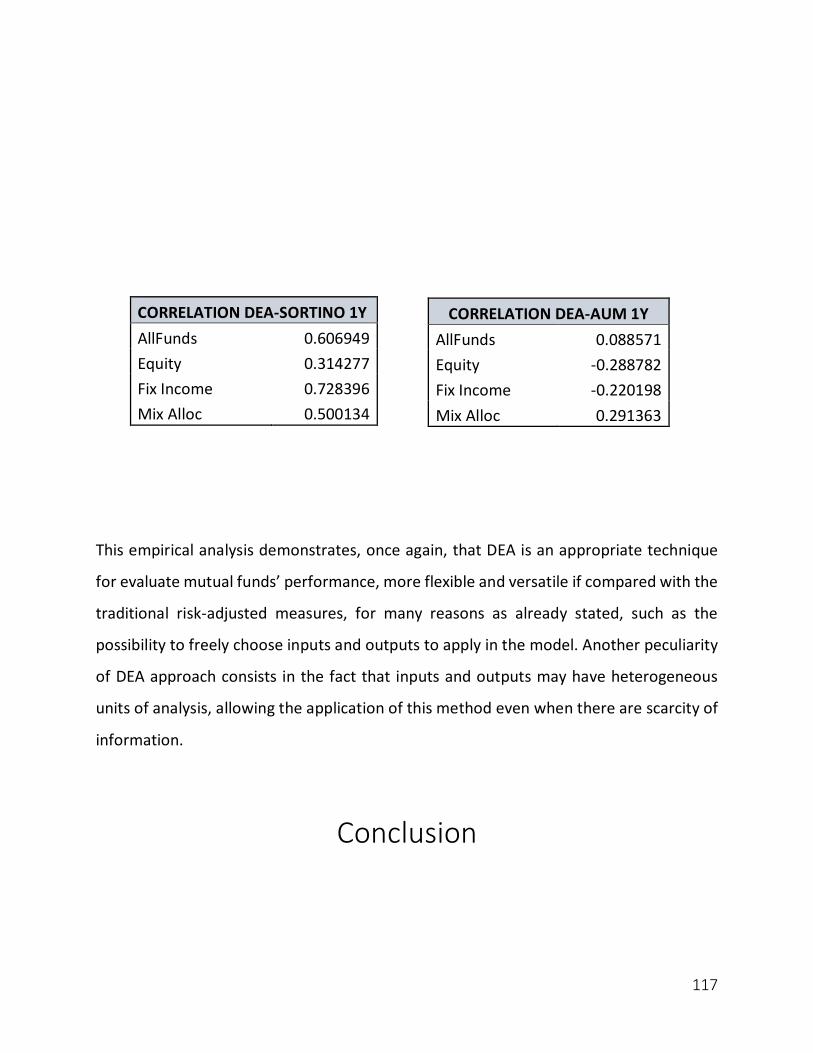
117

This empirical analysis demonstrates, once again, that DEA is an appropriate technique

for evaluate mutual funds’ performance, more flexible and versatile if compared with the

traditional risk-adjusted measures, for many reasons as already stated, such as the

possibility to freely choose inputs and outputs to apply in the model. Another peculiarity

of DEA approach consists in the fact that inputs and outputs may have heterogeneous

units of analysis, allowing the application of this method even when there are scarcity of

information.

Conclusion

CORRELATION DEA-AUM 1Y AllFunds 0.088571 Equity -0.288782 Fix Income -0.220198 Mix Alloc 0.291363

CORRELATION DEA-SORTINO 1Y AllFunds 0.606949 Equity 0.314277 Fix Income 0.728396 Mix Alloc 0.500134

118

In this thesis we have gone through a detailed analysis of every aspect of investment

funds. Starting from mere definitions and classifications, we presented the principal

traditional tools an investor can use to assess mutual funds’ performances. Furthermore,

introducing Data Envelopment Analysis, we provided a powerful instrument through

which is possible to make more detailed and user-adjustable analysis about funds’

efficiency. To conclude the analysis, it can be said that DEA has many advantages and

some drawbacks. First of all, it allows to consider several inputs and outputs, without the

need for them to have homogenous unit of analysis. This feature permits to analyze

performance from different perspective, focusing on various variables, and to apply DEA

even when there is lack of data.

Through the Murthi, Choe and Desai DEA model, we have seen how this powerful tool

allows to include the cost of owning a mutual fund share, in the form of expense ratio and

load charges, as input variable in addition to risk and return. It has been possible to

compute the efficiency for a sample of Italian investment funds, drawing up in this way a

rank of performance efficiency, which is compared with results based on traditional risk-

adjusted metrics, such as Sharpe and Sortino ratios, in order to evaluate the integrity of

DEA model.

The evaluation and comparison processes have been directed towards an empirical

assessment of transaction costs’ incidence over the total performance of mutual funds,

incidence that is not embedded in most used, and well-known, risk-adjusted measures.

Results have confirmed the validity of DEA technique as tool for measuring performance

of investment funds, highlighting that transaction’s costs on average don’t modify the

efficiency judgement expressed by traditional measures.

Finally, we have tested the correlation between DEA results and traditional performance

gauges, such as Sharpe and Sortino ratios, finding a positive correlation, confirming the

validity of DEA approach, characterized by unique features that makes it flexible and

119

versatile.

Bibliography

- Anderson S., J. Born, O. Schnusenberg, (2009), “Closed-end Funds, Exchange-

Traded Funds and Hedge Funds: Origin, Functions and Literature”.

120

- Banker R.D., R.F. Charnes, W.W. Cooper, (1984), “Some models for estimating

technical and scale inefficiencies in Data Envelopment Analysis”, Management

Science vol 30 no. 9, 1078-1092.

- Basso A., S. Funari, (2001), “A data envelopment analysis approach to measure the

mutual fund performance”, European Journal of Operational Research.

- Bodie B., A. Kane, A.J. Marcus, (2011), “Investments and Portfolio Management:

Global Edition”, McGraw-Hill, 9th Edition.

- Charnes A., W.W. Cooper, E. Rhodes, (1978), “Measuring the Efficiency of Decision-

Making Units”, European Journal of Operational Research.

- Charnes A., W.W. Cooper, B. Golany, L. Seiford, J. Stutz, (1985), “Foundations of

data envelopment analysis for Pareto-Koopmans efficient empirical production

functions”, Journal of Econometrics vol. 30, 91-107.

- Chegwidden B., J. Thomas, S. Davidoff, (2013), “Investment Funds in United States:

Regulatory Overview”, Practical Law Company.

- Cooper W.W., L.M. Seiford, J. Zhu, (2011), “Handbook on Data Envelopment

Analysis”, Springer, Boston.

- Cooper W.W., L. M. Seiford, K. Tone, (2005), “Introduction to Data Envelopment

Analysis and its uses: with DEA-Solver software and references”, Springer-Verlag.

- Corrigan A., P.C. Kaufman, (1987), “Understanding Money Market Funds”.

- Emrouznejad A., Parker B.R., Tavares G., (2008), “Evaluation of research in

efficiency and productivity: a survey and analysis of the first 30 years of scholarly

literature in DEA”. Socio-Economic Planning Sciences.

- Fama Eugene F., French Kenneth R., (1993), "Common Risk Factors in the Returns

on Stocks and Bonds", Journal of Financial Economics, February.

- Fama E. F., French K. R., “The Capital Asset Pricing Model: Theory and Evidence”,

Journal of Economic Perspectives, Volume 18.

121

- Farrell M. J., (1957), “The Measurement of Productive Efficiency”, Journal of Royal

Statistical Society.

- Fox W. P., (2017), “Mathematical Modeling for Business Analytics”, CRC Press.

- Gregariou G. N., Sedzro K., Zhu J. (2004), “Hedge fund performance appraisal using

data envelopment analysis”, European Journal of Operational Research.

- Gregoriou G. N. (2003), “Performance Appraisal of Funds of Hedge Funds Using

Data Envelopment Analysis”, Working Paper n. 5.

- Gregoriou G. N., Sedzro K., Zhu J., (2005), “Hedge Fund Performance Appraisal

Using Data Envelopment Analysis”.

- Grinblatt M., Titman S., (1993), “Performance Measurement without benchmarks:

An Examination of Mutual Fund Returns”, The Journal of Business, vol.66, issue 1,

47-68.

- Jensen M.C., (1968), “The Performance of Mutual Funds in the Period 1945-1964”.

Journal of Finance, 23, 389-416.

- Johns N., Howcroft B., Drake L., (197), “The use of data envelopment analysis to

monitor hotel productivity”, Progress in Tourism and Hospitality Research.

- Markowitz H. M., (1991), “Foundation of Portfolio Theory”, Journal of Finance,

Volume 46, Issue 2, 469-477

- Markowitz H.M., (1952) “Portfolio Selection”, Journal of Finance, 7, 77-91.

- Moloney N., (2015), “EU Securities and Financial Markets Regulation”, Oxford

University Press.

- Morey M. R., Morey R. C., (1998), “Mutual fund performance appraisals: a multi-

horizon perspective with endogenous benchmarking”, Omega, The International

Journal of Management Science vol. 27.

- Murthi B. P. S., Choi Y. K., Desai P., (1997), “Efficiency of mutual funds and portfolio

performance measurement: a non-parametric approach”, European Journal of

Operational Research vol. 98.

122

- Robertson R. A., (2001), “Fund Governance: Legal Duties of Investment Company”

Directors, Law Journal Press.

- Ross S., (1976), “The arbitrage theory of capital pricing”, Journal of Economic

Theory.

- Ruppel W., (2017), “Wiley GAAP for Governments 2017: Interpretation and

Application of Generally Accepted Accounting Principle for State and Local

Governments”, pp. 228-229

- Sharpe W.F., (1966), “Mutual Fund Performance”. Journal of Business, 1, 119-138.

- Sortino F. A., L.N. Price, (1994), “Performance measurement in a downside risk

framework”, Journal of Investing 3: 50–8.

- Steinki O., (2015), “Common Metric for Performance Evaluation: Overview of

popular Performance Measurement Ratios”, Evolutiq.

- Zhao Y., Triantis K., Murray-Tuite P., Edara P., (2011), “Performance measurement

of a transportation network with a downtown space reservation system: A

network-DEA system, Transportation Research Part E: Logistics and Transportation

Review”.

- Zhu J., (2016), “Data Envelopment Analysis: A Handbook of Empirical Studies and

Applications”, Springer, pp. 229-230.

Sitography

https://www.ecb.europa.eu/ecb/legal/pdf/l_21120070811en00080029.pdf

https://www.sec.gov/investor/pubs/sec-guide-to-mutual-funds.pdf

https://www.ici.org/research/stats/worldwide/ww_q3_17

http://eimf.eu/aif_ucits_seminar/

123

http://us.spindices.com/indices/equity/sp-500

http://www.assogestioni.it

http://www.morningstar.com

http://www.bloomberg.com