Performance evaluation model of streaming video in wireless mesh networks Juan Urrea Advisor Natalia Gaviria Faculty of Engineering University of Antioquia This dissertation is submitted for the degree of Doctor of Engineering June 2016

Welcome message from author
This document is posted to help you gain knowledge. Please leave a comment to let me know what you think about it! Share it to your friends and learn new things together.
Transcript
Performance evaluation model ofstreaming video in wireless mesh
networks
Juan Urrea
AdvisorNatalia Gaviria
Faculty of Engineering
University of Antioquia
This dissertation is submitted for the degree of
Doctor of Engineering
June 2016

Table of contents
List of figures 7
List of tables 11
1 Introduction 11.1 Application scenario: video streaming in wireless campus networks . . . . 3
1.1.1 Wireless mesh networks . . . . . . . . . . . . . . . . . . . . . . . 31.1.2 IEEE 802.11s mesh standard . . . . . . . . . . . . . . . . . . . . . 41.1.3 Network topology in the application scenario . . . . . . . . . . . . 5
1.2 Problem Statement . . . . . . . . . . . . . . . . . . . . . . . . . . . . . . 61.2.1 Objectives . . . . . . . . . . . . . . . . . . . . . . . . . . . . . . . 8
1.3 Thesis structure . . . . . . . . . . . . . . . . . . . . . . . . . . . . . . . . 8
2 Performance model for IEEE 802.11 multihop wireless networks 92.1 Introduction . . . . . . . . . . . . . . . . . . . . . . . . . . . . . . . . . . 92.2 Performance models for distributed wireless access . . . . . . . . . . . . . 11
2.2.1 IEEE 802.11 MAC Overview . . . . . . . . . . . . . . . . . . . . 112.3 Single hop MAC Layer analytical models - saturated . . . . . . . . . . . . 12
2.3.1 Decoupling Approximation in wireless networks . . . . . . . . . . 132.4 Singlehop MAC Layer analytical model - Unsaturated . . . . . . . . . . . . 162.5 Performance models in multihop wireless networks . . . . . . . . . . . . . 17
2.5.1 Related models . . . . . . . . . . . . . . . . . . . . . . . . . . . . 182.6 Background for the proposed MHWN model . . . . . . . . . . . . . . . . 20
2.6.1 Singlehop MAC Layer analytical model . . . . . . . . . . . . . . . 202.6.2 Unsaturated MAC Service Time . . . . . . . . . . . . . . . . . . . 212.6.3 Sensitivity analysis . . . . . . . . . . . . . . . . . . . . . . . . . . 232.6.4 M/G/1 queuing model . . . . . . . . . . . . . . . . . . . . . . . . 242.6.5 MAC Service time distribution . . . . . . . . . . . . . . . . . . . . 24
4 Table of contents
2.6.6 Throughput . . . . . . . . . . . . . . . . . . . . . . . . . . . . . . 252.6.7 Delay distribution . . . . . . . . . . . . . . . . . . . . . . . . . . . 25
2.7 Proposed performance model for MHWN . . . . . . . . . . . . . . . . . . 252.7.1 Multihop collision domain . . . . . . . . . . . . . . . . . . . . . . 262.7.2 Interference model . . . . . . . . . . . . . . . . . . . . . . . . . . 262.7.3 Graph model . . . . . . . . . . . . . . . . . . . . . . . . . . . . . 302.7.4 Multihop arrival rate . . . . . . . . . . . . . . . . . . . . . . . . . 322.7.5 Multihop fixed point approximation of collision probability . . . . 372.7.6 QoS metrics for the multihop performance model . . . . . . . . . . 37
2.8 Conclusions . . . . . . . . . . . . . . . . . . . . . . . . . . . . . . . . . . 39
3 Implementation and validation of the MHWN performance evaluation model 433.1 Introduction . . . . . . . . . . . . . . . . . . . . . . . . . . . . . . . . . . 433.2 Performance model algorithm . . . . . . . . . . . . . . . . . . . . . . . . 443.3 Experimental testbed . . . . . . . . . . . . . . . . . . . . . . . . . . . . . 513.4 Validation . . . . . . . . . . . . . . . . . . . . . . . . . . . . . . . . . . . 54
3.4.1 Throughput . . . . . . . . . . . . . . . . . . . . . . . . . . . . . . 573.4.2 Delay . . . . . . . . . . . . . . . . . . . . . . . . . . . . . . . . . 613.4.3 Jitter . . . . . . . . . . . . . . . . . . . . . . . . . . . . . . . . . 643.4.4 Validate QoS metrics in grid topologies with perturbations . . . . . 67
3.5 Conclusions . . . . . . . . . . . . . . . . . . . . . . . . . . . . . . . . . . 73
4 Performance evaluation model: validation in the application scenario 754.1 Introduction . . . . . . . . . . . . . . . . . . . . . . . . . . . . . . . . . . 754.2 Experimental testbed . . . . . . . . . . . . . . . . . . . . . . . . . . . . . 76
4.2.1 Poisson traffic validation . . . . . . . . . . . . . . . . . . . . . . . 784.2.2 Independence validation . . . . . . . . . . . . . . . . . . . . . . . 794.2.3 Self-similar validation . . . . . . . . . . . . . . . . . . . . . . . . 80
4.3 Validation . . . . . . . . . . . . . . . . . . . . . . . . . . . . . . . . . . . 814.3.1 Throughput . . . . . . . . . . . . . . . . . . . . . . . . . . . . . . 834.3.2 Delay . . . . . . . . . . . . . . . . . . . . . . . . . . . . . . . . . 864.3.3 Jitter . . . . . . . . . . . . . . . . . . . . . . . . . . . . . . . . . 89
4.4 Conclusions . . . . . . . . . . . . . . . . . . . . . . . . . . . . . . . . . . 93
5 Statistical performance evaluation of P2P video streaming on MHWN 955.1 Introduction . . . . . . . . . . . . . . . . . . . . . . . . . . . . . . . . . . 955.2 Streaming video quality evaluation . . . . . . . . . . . . . . . . . . . . . . 96
Table of contents 5
5.2.1 Quality from the application layer perspective . . . . . . . . . . . . 965.2.2 Quality from the MAC layer perspective . . . . . . . . . . . . . . . 97
5.3 Related work . . . . . . . . . . . . . . . . . . . . . . . . . . . . . . . . . 985.4 Statistical performance evaluation . . . . . . . . . . . . . . . . . . . . . . 99
5.4.1 Multi-variate regression analysis . . . . . . . . . . . . . . . . . . . 995.4.2 K-Means clustering . . . . . . . . . . . . . . . . . . . . . . . . . . 100
5.5 Experimental testbed . . . . . . . . . . . . . . . . . . . . . . . . . . . . . 1015.6 Results . . . . . . . . . . . . . . . . . . . . . . . . . . . . . . . . . . . . . 1025.7 Conclusions . . . . . . . . . . . . . . . . . . . . . . . . . . . . . . . . . . 107
6 Results and contributions 1116.1 Main contributions . . . . . . . . . . . . . . . . . . . . . . . . . . . . . . 111
6.1.1 Performance evaluation model of MHWN . . . . . . . . . . . . . . 1116.1.2 Validation methodology . . . . . . . . . . . . . . . . . . . . . . . 1126.1.3 Experimental unit of NS-3 MHWN simulation model . . . . . . . . 1136.1.4 Experimental unit of NS-3 MHWN emulation model . . . . . . . . 1146.1.5 Poisson process as an approximation of P2P video streaming . . . . 1146.1.6 Statistical performance evaluation of P2P video streaming on MHWN115
6.2 List of publications . . . . . . . . . . . . . . . . . . . . . . . . . . . . . . 1166.2.1 List of publications to be submitted . . . . . . . . . . . . . . . . . 117
References 119
Appendix A Statistical validation tables 131A.1 Throughput . . . . . . . . . . . . . . . . . . . . . . . . . . . . . . . . . . 131A.2 Delay . . . . . . . . . . . . . . . . . . . . . . . . . . . . . . . . . . . . . 136A.3 Jitter . . . . . . . . . . . . . . . . . . . . . . . . . . . . . . . . . . . . . . 145A.4 Statistical mean difference validation (G,GU [±10]) . . . . . . . . . . . . . . 156A.5 Statistical mean difference validation (G,GU [±20]) . . . . . . . . . . . . . . 168
Appendix B Performance model files list 181

List of figures
1.1 P2P streaming topology over a multihop wireless network. . . . . . . . . . 21.2 The open80211s stack into the Linux kernel [1]. . . . . . . . . . . . . . . . 41.3 Three regular grid topologies [2] . . . . . . . . . . . . . . . . . . . . . . . 51.4 Quality metrics for the streaming topology (QoS-QoE). . . . . . . . . . . . 7
2.1 Performance model validation. . . . . . . . . . . . . . . . . . . . . . . . . 102.2 DCF flow diagram . . . . . . . . . . . . . . . . . . . . . . . . . . . . . . 122.3 DTMC of Binary Exponential Backoff [3] . . . . . . . . . . . . . . . . . . 142.4 Channel events process example [4] . . . . . . . . . . . . . . . . . . . . . 142.5 Evolution of the back-offs of a node. Each attempted packet starts a new
back-off cycle [5]. . . . . . . . . . . . . . . . . . . . . . . . . . . . . . . . 202.6 Plots of γ(β ,λ ) and γ(βc) versus γ [6]. . . . . . . . . . . . . . . . . . . . . 232.7 Proposed performance evaluation model for a multihop wireless node. . . . 252.8 Multihop collision domain. . . . . . . . . . . . . . . . . . . . . . . . . . . 262.9 Hidden node effect. Node A cannot hear node C and vice-versa. . . . . . . 272.10 A multihop path between a given source S and the destination D. The carrier
sensing range of each node is twice of the transmission range [7]. . . . . . . 272.11 Common area between the carrier sense ranges of two adjacent nodes with a
distance between their centers t = r [7]. . . . . . . . . . . . . . . . . . . . 282.12 Possible application scenario topology for a wireless campus network. . . . 302.13 Interference model description. . . . . . . . . . . . . . . . . . . . . . . . . 322.14 Multihop and single hop topologies . . . . . . . . . . . . . . . . . . . . . 332.15 λmh and HC as a function of grid topologies. . . . . . . . . . . . . . . . . . 342.16 nmh as a function of n nodes in a grid topology. . . . . . . . . . . . . . . . 342.17 Topology model description. . . . . . . . . . . . . . . . . . . . . . . . . . 352.18 Queue and traffic model description. . . . . . . . . . . . . . . . . . . . . . 372.19 Multihop model FPA description. . . . . . . . . . . . . . . . . . . . . . . . 382.20 QoS metrics description . . . . . . . . . . . . . . . . . . . . . . . . . . . . 39
8 List of figures
3.1 MHWN performance evaluation model. . . . . . . . . . . . . . . . . . . . 433.2 Validation process between performance model and simulation model. . . . 443.3 Performance model flow diagram (Alg. 6). . . . . . . . . . . . . . . . . . . 453.4 Topology model implemented. . . . . . . . . . . . . . . . . . . . . . . . . 453.5 Interference model implemented. . . . . . . . . . . . . . . . . . . . . . . . 463.6 Queue model implemented. . . . . . . . . . . . . . . . . . . . . . . . . . . 463.7 Multihop FPA model implemented. . . . . . . . . . . . . . . . . . . . . . . 493.8 QoS metrics implemented. . . . . . . . . . . . . . . . . . . . . . . . . . . 493.9 Single node experimental testbed stack. . . . . . . . . . . . . . . . . . . . 513.10 Network topologies implemented. . . . . . . . . . . . . . . . . . . . . . . 553.11 Detailed validation process between performance model and simulation model. 563.12 Analytical and simulated throughput for λ = 10 . . . . . . . . . . . . . . . 583.13 Analytical and simulated throughput for λ = 50 . . . . . . . . . . . . . . . 593.14 Analytical and simulated throughput for λ = 100 . . . . . . . . . . . . . . 593.15 Analytical and simulated throughput for λ = 200 . . . . . . . . . . . . . . 603.16 Analytical and simulated delay for λ = 10 . . . . . . . . . . . . . . . . . . 613.17 Analytical and simulated delay for λ = 50 . . . . . . . . . . . . . . . . . . 623.18 Analytical and simulated delay for λ = 100 . . . . . . . . . . . . . . . . . 633.19 Analytical and simulated delay for λ = 200 . . . . . . . . . . . . . . . . . 643.20 Analytical and simulated jitter for λ = 10 . . . . . . . . . . . . . . . . . . 643.21 Analytical and simulated jitter for λ = 50 . . . . . . . . . . . . . . . . . . 653.22 Analytical and simulated jitter for λ = 100 . . . . . . . . . . . . . . . . . . 653.23 Analytical and simulated jitter for λ = 150 . . . . . . . . . . . . . . . . . . 653.24 Analytical and simulated jitter for λ = 200 . . . . . . . . . . . . . . . . . . 663.25 Validation process between grid topologies with and without perturbations. 683.26 Perturbed grid topologies for Xr,Yr ∼U [−10,10]. . . . . . . . . . . . . . . 693.27 Perturbed grid topologies for Xr,Yr ∼U [−20,20]. . . . . . . . . . . . . . . 70
4.1 Validation process between performance model and emulation model. . . . 764.2 Single node experimental testbed stack. . . . . . . . . . . . . . . . . . . . 774.3 Topologies implemented . . . . . . . . . . . . . . . . . . . . . . . . . . . 784.4 Interarrival times for three nodes in akiyo video. . . . . . . . . . . . . . . . 794.5 Coefficient of variation and Lag 1 autocorrelation value for three videos. . . 794.6 Estimated Hurst parameters for three videos. . . . . . . . . . . . . . . . . . 804.7 Selected videos for real-time emulation. . . . . . . . . . . . . . . . . . . . 814.8 Detailed validation process between performance model and emulation model. 824.9 Analytical and emulated throughput for video akiyo . . . . . . . . . . . . . 83
List of figures 9
4.10 Analytical and emulated throughput for video bigbuck . . . . . . . . . . . 834.11 Analytical and emulated throughput for video foreman . . . . . . . . . . . 854.12 Analytical and emulated throughput for video bridge . . . . . . . . . . . . 854.13 Analytical and emulated throughput for video highway . . . . . . . . . . . 854.14 Analytical and emulated delay for video bigbuck . . . . . . . . . . . . . . 874.15 Analytical and emulated delay for video foreman . . . . . . . . . . . . . . 874.16 Analytical and emulated delay for video highway . . . . . . . . . . . . . . 884.17 Analytical and emulated jitter for video akiyo . . . . . . . . . . . . . . . . 904.18 Analytical and emulated jitter for video bridge . . . . . . . . . . . . . . . . 904.19 Analytical and emulated jitter for video highway . . . . . . . . . . . . . . 90
5.1 QoE metric used: PSQA [158] . . . . . . . . . . . . . . . . . . . . . . . . 975.2 Statistical performance evaluation proposed. . . . . . . . . . . . . . . . . . 1015.3 K-means WSSK increasing the number of clusters . . . . . . . . . . . . . . 1055.4 Clustering with two principal components. . . . . . . . . . . . . . . . . . . 1065.5 Regression conditions for the throughput model. . . . . . . . . . . . . . . . 1095.6 Regression conditions for the delay model. . . . . . . . . . . . . . . . . . . 1095.7 Regression conditions for the jitter model. . . . . . . . . . . . . . . . . . . 1105.8 Regression conditions for the QoE model. . . . . . . . . . . . . . . . . . . 110
6.1 Proposed performance evaluation model for a multihop wireless node. . . . 1116.2 Performance model flow diagram (Alg. 6). . . . . . . . . . . . . . . . . . . 1126.3 Detailed validation process between performance model and simulation model.1136.4 Validation process between grid topologies with and without perturbations. 1136.5 Single node experimental testbed stack. . . . . . . . . . . . . . . . . . . . 1146.6 Single node experimental testbed stack. . . . . . . . . . . . . . . . . . . . 1156.7 Detailed validation process between performance model and emulation model.1156.8 Statistical performance evaluation proposed. . . . . . . . . . . . . . . . . . 116
B.1 Performance model files tree. . . . . . . . . . . . . . . . . . . . . . . . . . 181B.2 Performance model functions tree. . . . . . . . . . . . . . . . . . . . . . . 182

List of tables
3.1 NS-3 MHWN simulation parameters . . . . . . . . . . . . . . . . . . . . . 533.2 IEEE 802.11a parameters in NS-3 . . . . . . . . . . . . . . . . . . . . . . 533.3 Set of input parameters . . . . . . . . . . . . . . . . . . . . . . . . . . . . 543.4 Simulation times . . . . . . . . . . . . . . . . . . . . . . . . . . . . . . . 563.5 Percentage of accepted H0 for Throughput (AODV). . . . . . . . . . . . . . 583.6 Percentage of accepted H0 for Throughput (HWMP). . . . . . . . . . . . . 603.7 Percentage of rejected H0 for Delay (AODV). . . . . . . . . . . . . . . . . 623.8 Percentage of rejected H0 for Delay (HWMP). . . . . . . . . . . . . . . . . 633.9 Percentage of rejected H0 for Jitter (AODV). . . . . . . . . . . . . . . . . . 663.10 Percentage of rejected H0 for Jitter (HWMP). . . . . . . . . . . . . . . . . 673.11 Percentage of p-values accepting H0, in GU [±10] vs. G (AODV) . . . . . . . 713.12 Percentage of p-values accepting H0, in GU [±10] vs. G (HWMP) . . . . . . 713.13 Percentage of p-values accepting H0, in GU [±20] vs. G (AODV). . . . . . . 723.14 Percentage of p-values accepting H0, in GU [±20] vs. G (HWMP). . . . . . . 72
4.1 Emulation parameters . . . . . . . . . . . . . . . . . . . . . . . . . . . . . 774.2 R commands used for Hurst’s parameter estimation. . . . . . . . . . . . . . 804.3 Set of variable emulation parameters . . . . . . . . . . . . . . . . . . . . . 814.4 Throughput statistics for T-test (AODV). . . . . . . . . . . . . . . . . . . . 844.5 Throughput statistics for T-test (HWMP). . . . . . . . . . . . . . . . . . . 864.6 Delay statistics for T-test (AODV). . . . . . . . . . . . . . . . . . . . . . . 884.7 Delay statistics for T-test (HWMP). . . . . . . . . . . . . . . . . . . . . . 894.8 Jitter statistics for T-test (AODV). . . . . . . . . . . . . . . . . . . . . . . 914.9 Jitter statistics for T-test (HWMP). . . . . . . . . . . . . . . . . . . . . . . 92
5.1 Factors selected for the experiment . . . . . . . . . . . . . . . . . . . . . . 1005.2 Regresion model for Throughput. R2 = 0.7620 . . . . . . . . . . . . . . . 1035.3 Reduced regression model for Throughput. R2 = 0.7598. . . . . . . . . . . 103
12 List of tables
5.4 Delay Regresion model. R2 = 0.6544. . . . . . . . . . . . . . . . . . . . . 1045.5 Jitter Regresion model. R2 = 0.6940. . . . . . . . . . . . . . . . . . . . . . 1045.6 QoE Regresion model. R2 = 0.8227 . . . . . . . . . . . . . . . . . . . . . 1045.7 Five centroids generated by K-means ordered by QoE. . . . . . . . . . . . 1065.8 Importance of components. . . . . . . . . . . . . . . . . . . . . . . . . . . 1065.9 Variables contributions to principal components. . . . . . . . . . . . . . . 107
A.1 Percentage of accepted H0 for Throughput (AODV). . . . . . . . . . . . . . 131A.2 Throughput statistics for λ = 10 and packet size of 256 bytes. . . . . . . . 132A.3 Throughput statistics for λ = 10 and packet size of 512 bytes. . . . . . . . 132A.4 Throughput statistics for λ = 10 and packet size of 1024 bytes. . . . . . . . 132A.5 Throughput statistics for λ = 50 and packet size of 256 bytes. . . . . . . . 133A.6 Throughput statistics for λ = 50 and packet size of 512 bytes. . . . . . . . 133A.7 Throughput statistics for λ = 50 and packet size of 1024 bytes. . . . . . . . 133A.8 Throughput statistics for λ = 100 and packet size of 256 bytes. . . . . . . . 134A.9 Throughput statistics for λ = 100 and packet size of 512 bytes. . . . . . . . 134A.10 Throughput statistics for λ = 100 and packet size of 1024 bytes. . . . . . . 134A.11 Throughput statistics for λ = 200 and packet size of 256 bytes. . . . . . . . 135A.12 Throughput statistics for λ = 200 and packet size of 512 bytes. . . . . . . . 135A.13 Throughput statistics for λ = 200 and packet size of 1024 bytes. . . . . . . 135A.14 Percentage of accepted H0 for Delay (AODV). . . . . . . . . . . . . . . . . 136A.15 Delay statistics for λ = 10 and packet size of 256 bytes. . . . . . . . . . . 137A.16 Delay statistics for λ = 10 and packet size of 512 bytes. . . . . . . . . . . 137A.17 Delay statistics for λ = 10 and packet size of 1024 bytes. . . . . . . . . . . 138A.18 Delay statistics for λ = 50 and packet size of 256 bytes. . . . . . . . . . . 139A.19 Delay statistics for λ = 50 and packet size of 512 bytes. . . . . . . . . . . 139A.20 Delay statistics for λ = 50 and packet size of 1024 bytes. . . . . . . . . . . 140A.21 Delay statistics for λ = 100 and packet size of 256 bytes. . . . . . . . . . . 141A.22 Delay statistics for λ = 100 and packet size of 512 bytes. . . . . . . . . . . 141A.23 Delay statistics for λ = 100 and packet size of 1024 bytes. . . . . . . . . . 142A.24 Delay statistics for λ = 200 and packet size of 256 bytes. . . . . . . . . . . 143A.25 Delay statistics for λ = 200 and packet size of 512 bytes. . . . . . . . . . . 143A.26 Delay statistics for λ = 200 and packet size of 1024 bytes. . . . . . . . . . 144A.27 Percentage of rejected H0 for Jitter (AODV). . . . . . . . . . . . . . . . . . 145A.28 Jitter statistics for λ = 10 and packet size of 256 bytes. . . . . . . . . . . . 146A.29 Jitter statistics for λ = 10 and packet size of 512 bytes. . . . . . . . . . . . 146A.30 Jitter statistics for λ = 10 and packet size of 1024 bytes. . . . . . . . . . . 147
List of tables 13
A.31 Jitter statistics for λ = 50 and packet size of 256 bytes. . . . . . . . . . . . 148A.32 Jitter statistics for λ = 50 and packet size of 512 bytes. . . . . . . . . . . . 148A.33 Jitter statistics for λ = 50 and packet size of 1024 bytes. . . . . . . . . . . 149A.34 Jitter statistics for λ = 100 and packet size of 256 bytes. . . . . . . . . . . 150A.35 Jitter statistics for λ = 100 and packet size of 512 bytes. . . . . . . . . . . 150A.36 Jitter statistics for λ = 100 and packet size of 1024 bytes. . . . . . . . . . . 151A.37 Jitter statistics for λ = 150 and packet size of 64 bytes. . . . . . . . . . . . 152A.38 Jitter statistics for λ = 150 and packet size of 256 bytes. . . . . . . . . . . 152A.39 Jitter statistics for λ = 150 and packet size of 512 bytes. . . . . . . . . . . 153A.40 Jitter statistics for λ = 200 and packet size of 64 bytes. . . . . . . . . . . . 154A.41 Jitter statistics for λ = 200 and packet size of 256 bytes. . . . . . . . . . . 154A.42 Jitter statistics for λ = 200 and packet size of 512 bytes. . . . . . . . . . . 155A.43 Throughput statistics for G and GU [±10] topologies (λ = 10 ,p= 256 ) . . . . 156A.44 Throughput statistics for G and GU [±10] topologies (λ = 10 ,p= 512 ) . . . . 156A.45 Throughput statistics for G and GU [±10] topologies (λ = 10 ,p= 1024 ) . . . 156A.46 Throughput statistics for G and GU [±10] topologies (λ = 50 ,p= 256 ) . . . . 157A.47 Throughput statistics for G and GU [±10] topologies (λ = 50 ,p= 512 ) . . . . 157A.48 Throughput statistics for G and GU [±10] topologies (λ = 50 ,p= 1024 ) . . . 157A.49 Throughput statistics for G and GU [±10] topologies (λ = 100 ,p= 256 ) . . . 158A.50 Throughput statistics for G and GU [±10] topologies (λ = 100 ,p= 512 ) . . . 158A.51 Throughput statistics for G and GU [±10] topologies (λ = 100 ,p= 1024 ) . . 158A.52 Throughput statistics for G and GU [±10] topologies (λ = 200 ,p= 256 ) . . . 159A.53 Throughput statistics for G and GU [±10] topologies (λ = 200 ,p= 512 ) . . . 159A.54 Throughput statistics for G and GU [±10] topologies (λ = 200 ,p= 1024 ) . . 159A.55 Delay statistics for G and GU [±10] topologies (λ = 10 ,p= 256 ) . . . . . . . 160A.56 Delay statistics for G and GU [±10] topologies (λ = 10 ,p= 512 ) . . . . . . . 160A.57 Delay statistics for G and GU [±10] topologies (λ = 10 ,p= 1024 ) . . . . . . 160A.58 Delay statistics for G and GU [±10] topologies (λ = 50 ,p= 256 ) . . . . . . . 161A.59 Delay statistics for G and GU [±10] topologies (λ = 50 ,p= 512 ) . . . . . . . 161A.60 Delay statistics for G and GU [±10] topologies (λ = 50 ,p= 1024 ) . . . . . . 161A.61 Delay statistics for G and GU [±10] topologies (λ = 100 ,p= 256 ) . . . . . . 162A.62 Delay statistics for G and GU [±10] topologies (λ = 100 ,p= 512 ) . . . . . . 162A.63 Delay statistics for G and GU [±10] topologies (λ = 100 ,p= 1024 ) . . . . . 162A.64 Delay statistics for G and GU [±10] topologies (λ = 200 ,p= 256 ) . . . . . . 163A.65 Delay statistics for G and GU [±10] topologies (λ = 200 ,p= 512 ) . . . . . . 163A.66 Delay statistics for G and GU [±10] topologies (λ = 200 ,p= 1024 ) . . . . . 163
14 List of tables
A.67 Jitter statistics for G and GU [±10] topologies (λ = 10 ,p= 256 ) . . . . . . . 164A.68 Jitter statistics for G and GU [±10] topologies (λ = 10 ,p= 512 ) . . . . . . . 164A.69 Jitter statistics for G and GU [±10] topologies (λ = 10 ,p= 1024 ) . . . . . . . 164A.70 Jitter statistics for G and GU [±10] topologies (λ = 50 ,p= 256 ) . . . . . . . 165A.71 Jitter statistics for G and GU [±10] topologies (λ = 50 ,p= 512 ) . . . . . . . 165A.72 Jitter statistics for G and GU [±10] topologies (λ = 50 ,p= 1024 ) . . . . . . . 165A.73 Jitter statistics for G and GU [±10] topologies (λ = 100 ,p= 256 ) . . . . . . . 166A.74 Jitter statistics for G and GU [±10] topologies (λ = 100 ,p= 512 ) . . . . . . . 166A.75 Jitter statistics for G and GU [±10] topologies (λ = 100 ,p= 1024 ) . . . . . . 166A.76 Jitter statistics for G and GU [±10] topologies (λ = 200 ,p= 256 ) . . . . . . . 167A.77 Jitter statistics for G and GU [±10] topologies (λ = 200 ,p= 512 ) . . . . . . . 167A.78 Jitter statistics for G and GU [±10] topologies (λ = 200 ,p= 1024 ) . . . . . . 167A.79 Throughput statistics for G and GU [±20] topologies (λ = 10 ,p= 256 ) . . . . 168A.80 Throughput statistics for G and GU [±20] topologies (λ = 10 ,p= 512 ) . . . . 168A.81 Throughput statistics for G and GU [±20] topologies (λ = 10 ,p= 1024 ) . . . 168A.82 Throughput statistics for G and GU [±20] topologies (λ = 50 ,p= 256 ) . . . . 169A.83 Throughput statistics for G and GU [±20] topologies (λ = 50 ,p= 512 ) . . . . 169A.84 Throughput statistics for G and GU [±20] topologies (λ = 50 ,p= 1024 ) . . . 169A.85 Throughput statistics for G and GU [±20] topologies (λ = 100 ,p= 256 ) . . . 170A.86 Throughput statistics for G and GU [±20] topologies (λ = 100 ,p= 512 ) . . . 170A.87 Throughput statistics for G and GU [±20] topologies (λ = 100 ,p= 1024 ) . . 170A.88 Throughput statistics for G and GU [±20] topologies (λ = 200 ,p= 256 ) . . . 171A.89 Throughput statistics for G and GU [±20] topologies (λ = 200 ,p= 512 ) . . . 171A.90 Throughput statistics for G and GU [±20] topologies (λ = 200 ,p= 1024 ) . . 171A.91 Delay statistics for G and GU [±20] topologies (λ = 10 ,p= 256 ) . . . . . . . 172A.92 Delay statistics for G and GU [±20] topologies (λ = 10 ,p= 512 ) . . . . . . . 172A.93 Delay statistics for G and GU [±20] topologies (λ = 10 ,p= 1024 ) . . . . . . 172A.94 Delay statistics for G and GU [±20] topologies (λ = 50 ,p= 256 ) . . . . . . . 173A.95 Delay statistics for G and GU [±20] topologies (λ = 50 ,p= 512 ) . . . . . . . 173A.96 Delay statistics for G and GU [±20] topologies (λ = 50 ,p= 1024 ) . . . . . . 173A.97 Delay statistics for G and GU [±20] topologies (λ = 100 ,p= 256 ) . . . . . . 174A.98 Delay statistics for G and GU [±20] topologies (λ = 100 ,p= 512 ) . . . . . . 174A.99 Delay statistics for G and GU [±20] topologies (λ = 100 ,p= 1024 ) . . . . . 174A.100Delay statistics for G and GU [±20] topologies (λ = 200 ,p= 256 ) . . . . . . 175A.101Delay statistics for G and GU [±20] topologies (λ = 200 ,p= 512 ) . . . . . . 175A.102Delay statistics for G and GU [±20] topologies (λ = 200 ,p= 1024 ) . . . . . 175

List of tables 15
A.103Jitter statistics for G and GU [±20] topologies (λ = 10 ,p= 256 ) . . . . . . . 176A.104Jitter statistics for G and GU [±20] topologies (λ = 10 ,p= 512 ) . . . . . . . 176A.105Jitter statistics for G and GU [±20] topologies (λ = 10 ,p= 1024 ) . . . . . . . 176A.106Jitter statistics for G and GU [±20] topologies (λ = 50 ,p= 256 ) . . . . . . . 177A.107Jitter statistics for G and GU [±20] topologies (λ = 50 ,p= 512 ) . . . . . . . 177A.108Jitter statistics for G and GU [±20] topologies (λ = 50 ,p= 1024 ) . . . . . . . 177A.109Jitter statistics for G and GU [±20] topologies (λ = 100 ,p= 256 ) . . . . . . . 178A.110Jitter statistics for G and GU [±20] topologies (λ = 100 ,p= 512 ) . . . . . . . 178A.111Jitter statistics for G and GU [±20] topologies (λ = 100 ,p= 1024 ) . . . . . . 178A.112Jitter statistics for G and GU [±20] topologies (λ = 200 ,p= 256 ) . . . . . . . 179A.113Jitter statistics for G and GU [±20] topologies (λ = 200 ,p= 512 ) . . . . . . . 179A.114Jitter statistics for G and GU [±20] topologies (λ = 200 ,p= 1024 ) . . . . . . 179


Chapter 1
Introduction
Over the past years, video streaming has become an important way to share. Communicationthrough video streaming is now part of our daily tasks at different levels such as information,entertainment, and education. Even it is a business in itself. Thanks to communicationnetworks we can access video content anytime, anywhere. From large enterprises offeringmovies and TV series to user generated content freely available, we can easily produce andshare a large amount of information, with just a few clicks.
Generally, videos are streamed to end users directly from the video server, or indirectlyfrom edge servers in a Content Delivery Network (CDN). Another popular streaming serviceis VoD, enabling almost immediate distribution of video to users, from any point of thecontent. Therefore the content distribution is expected to be one of the main applicationsof the future Internet [8]. By 2019, IP video traffic will be 80% of all IP traffic, and thesum of all forms of video (TV, video on demand (VoD), Internet, and P2P) will be between80%-90% of global consumer traffic [9].
Traditional streaming architectures provide good performance if the number of clientsis limited. However, the deployment and maintenance cost of these schemes is usuallyhigh [10], and the video distribution imposes challenges on communication networks [11].Besides, most of the streaming applications are designed to operate over wired networks.
Peer-to-Peer (P2P) video streaming has recently been used as an alternative with lowserver infrastructure cost and good scalability [11]. Under certain circumstances, a largeaudience saturates the client-server approach, due to servers with limited resources andscalability problems. Similarly, CDNs only scale with more servers and high infrastructurecosts. IP-Multicast presents lack of deployment for TV service on Internet [12].
Streaming services have become very accessible, with the integration of wireless commu-nication interfaces in a wide number of devices. By 2019, the expected traffic through Wi-Fiand mobile devices will be 81% of Internet traffic [9]. Electronic devices like tablets, laptops,
2 Introduction
smart-phones, video game consoles, and smart TVs, incorporate wireless network interfacesand video codecs to create and share video contents. Wireless access points have becomeubiquitous around corporate and academic campuses. Besides, the increasing number ofPublic Wi-Fi and community hotspots enable a higher access to video streaming and otherservices [9].
P2P Overlay Network
802.11 MAC Layer Network
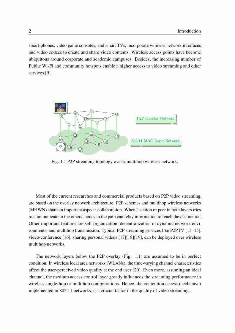
Fig. 1.1 P2P streaming topology over a multihop wireless network.
Most of the current researches and commercial products based on P2P video streaming,are based on the overlay network architecture. P2P schemes and multihop wireless networks(MHWN) share an important aspect: collaboration. When a station or peer in both layers triesto communicate to the others, nodes in the path can relay information to reach the destination.Other important features are self-organization, decentralization in dynamic network envi-ronments, and multihop transmission. Typical P2P streaming services like P2PTV [13–15],video-conference [16], sharing personal videos [17][18][19], can be deployed over wirelessmultihop networks.
The network layers below the P2P overlay (Fig. 1.1) are assumed to be in perfectcondition. In wireless local area networks (WLANs), the time-varying channel characteristicsaffect the user-perceived video quality at the end user [20]. Even more, assuming an idealchannel, the medium access control layer greatly influences the streaming performance inwireless single-hop or multihop configurations. Hence, the contention access mechanismimplemented in 802.11 networks, is a crucial factor in the quality of video streaming .
1.1 Application scenario: video streaming in wireless campus networks 3
1.1 Application scenario: video streaming in wireless cam-pus networks
Wireless networks have an important role in development of sustainable cities. Aspects suchas virtual education, smart cities, and energy efficiency, require technological support to theincreasing number of connected devices.
In recent years, enterprises and educational institutions are under an increasing pressurein order to provide access to applications and data. In campus networks, users access servicesand applications from anywhere and at any time. Laptops, smartphones and tablets proliferatein campus environments, and in such networks, their connectivity is based on the integrationof multiple WLANs.
The wireless network infrastructure concentrates most of the generated traffic required byusers, considering factors such as mobility of users, number of users and traffic consumption.However, the unreliable nature of the wireless medium requires more traffic control thanwired networks.
There are situations where connectivity solutions, based on wireless networks, presentproblems when providing adequate quality levels. The growing number of users leads thewireless network to a saturation state, yielding to more wireless access points, generatingmore costs and complexity in its administration.
1.1.1 Wireless mesh networks
Wireless mesh networks (WMN) is a replacement technology for last-mile connectivity tohome, office, community and public networking. A WMN is formed by routers or meshstations (mesh STA) and mesh clients, and each node in the network receive or forwardpackets to other nodes through a multihop transmission path [21][22]. The functionality ofgateway in mesh STA enable integration with various wireless technologies such as cellular,wireless sensor networks (WSN), Wi-Fi and Wi-MAX [23] [24]. WMNs are decentralized,easy to deploy, and characterized by dynamic self-organization, self-configuration, andself-healing properties [22].
Typical applications
Common WLAN mesh networks are deployed in enterprise, office, public and university cam-pus. WLAN mesh networks can also be used for large-sized warehouses, ports, metropolitanarea networks, rail transit, and emergent communications.
4 Introduction
Several communities have implemented WMNs for Internet access, educational purposes,and e-commerce [21][25][26][27][28] [29][30] [31], with the vision to reduce the DigitalDivide. A collaborative model of community network is implemented in [32], where eachnode aggregate Internet access. In [33] the authors present a survey of several rural IEEE802.11-based WMNs deployments. An application of WMN in emergency situations ispresented in [34], using a Linux Live USB flash drive.
Large WMNs have been implemented in community networks like MIT Roofnet [35],Berlin Roof Net [36], Freifunk [37], FunkFeuer [38], Microsoft Research [39], TFA Houston[40], CUWiN [41], among others. These networks are used to share the cost of Internetaccess, but also to support the distribution of community information and other services [42].
Besides, WMNs for research experimentation have been implemented, like MeshNet[43], Mesh@Purdue [44], Hyacinth [45], the Miniaturized Network Testbed (MiNT) [46],BWN-Mesh [47], Open Access Research Testbed for Next-Generation Wireless Networks(ORBIT) [48], the UCSB Meshnet [49], and UltraHigh Speed Mobile Information andCommunication (UMIC) [50].
Even software defined networking (SDN) has been deployed recently in WMN simplify-ing the network management. SDN paradigm separates control plane and data plane enablingflexible control and dynamic resource configuration [51][52][53][54][55].
1.1.2 IEEE 802.11s mesh standard
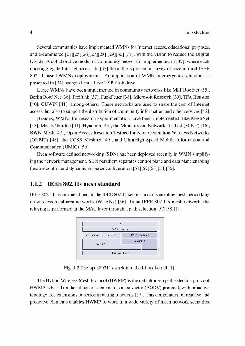
IEEE 802.11s is an amendment to the IEEE 802.11 set of standards enabling mesh networkingon wireless local area networks (WLANs) [56]. In an IEEE 802.11s mesh network, therelaying is performed at the MAC layer through a path selection [57][58][1].
Fig. 1.2 The open80211s stack into the Linux kernel [1].
The Hybrid Wireless Mesh Protocol (HWMP) is the default mesh path selection protocol.HWMP is based on the ad hoc on-demand distance vector (AODV) protocol, with proactivetopology tree extensions to perform routing functions [57]. This combination of reactive andproactive elements enables HWMP to work in a wide variety of mesh network scenarios.
1.1 Application scenario: video streaming in wireless campus networks 5
The IEEE 802.11s also introduces a set of frames and information elements (IEs). The frameextension includes a mesh header two additional MAC addresses, allowing legacy stations toaccess the mesh network [22].
Mesh routers can be implemented on general-purpose laptops, desktops or dedicatedsystems [59]. Linux kernels from version 2.6 have already implemented a wireless multihopprotocol [60], based on the IEEE 802.11s amendment, enabling the creation of WMNtopologies with laptops. Routers and embedded systems can also be used to implementwireless multihop networks using OpenWRT, an open source Linux distribution designedfor network embedded systems [61][62][63][64] [65]. Also, commercial wireless devices(like Microtik [66], HP [67], Fortinet [68], Extreme networks [69], Aruba networks [70])have adopted the mesh protocol, including high throughput rates with the 802.11n standard.Similar approaches have been developed for android based smart-phones [71], in a fullydecentralized peer connection.
1.1.3 Network topology in the application scenario
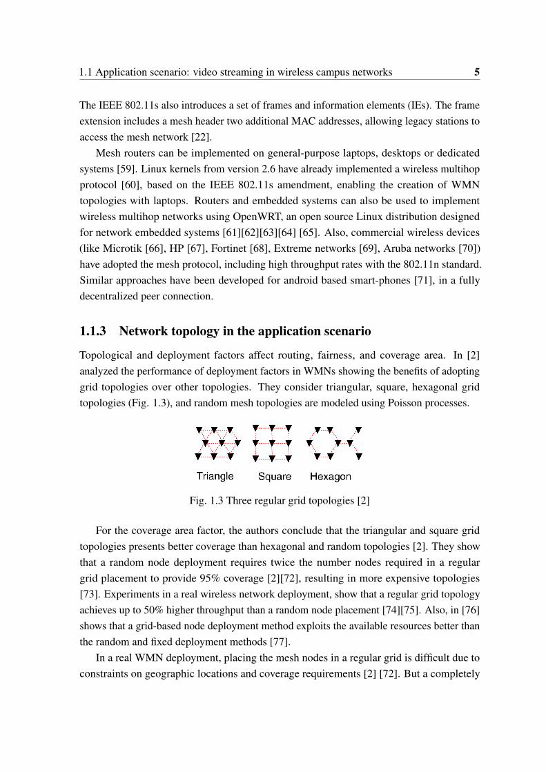
Topological and deployment factors affect routing, fairness, and coverage area. In [2]analyzed the performance of deployment factors in WMNs showing the benefits of adoptinggrid topologies over other topologies. They consider triangular, square, hexagonal gridtopologies (Fig. 1.3), and random mesh topologies are modeled using Poisson processes.
Fig. 1.3 Three regular grid topologies [2]
For the coverage area factor, the authors conclude that the triangular and square gridtopologies presents better coverage than hexagonal and random topologies [2]. They showthat a random node deployment requires twice the number nodes required in a regulargrid placement to provide 95% coverage [2][72], resulting in more expensive topologies[73]. Experiments in a real wireless network deployment, show that a regular grid topologyachieves up to 50% higher throughput than a random node placement [74][75]. Also, in [76]shows that a grid-based node deployment method exploits the available resources better thanthe random and fixed deployment methods [77].
In a real WMN deployment, placing the mesh nodes in a regular grid is difficult due toconstraints on geographic locations and coverage requirements [2] [72]. But a completely
6 Introduction
random placement decrease the availability compared to a grid placement, as mentionedbefore. In [2] each mesh node in a regular grid is displaced, a random distance and angle,resulting in a low influence on coverage area. Such scenario is evaluated in [77], where anincreased connectivity requires higher node density in real world deployments.
In urban-scale, enterprise and campus mesh networks it is possible a grid node placementdue to the availability of a large number of locations like office buildings, square parks, halls,etc.
1.2 Problem Statement
Today campus networks implement connectivity through wireless mesh networks. The costof extending the wireless infrastructures through mesh configuration are lower than othersolutions available. Wireless device vendors offer plenty of solutions focused in education[78][79][80][81][66][67][68][69][70]. Typical applications are:
• Video-Surveillance
• Voice and Video Streaming
• E-learning
• Wi-Fi
• Video-conference
In the case of virtual education, a live video is delivered to wireless users, e.g., the livecoverage of a cultural event, concert, conference, instructional video, or a prerecorded video[82]. With the implementation of a campus WMN, it is possible to stream live video andincrease the coverage in academic, cultural and institutional events [83].
In this work the application scenario is a virtual education or e-learning system. Thelecture is transmitted through P2P streaming video over IEEE 802.11s mesh campus network(corporate, university, college, community, public WMN), in a regular grid topology.
With the previous context three questions have arisen, in the development of this thesis:
1. ¿What are the principal factors that influence the quality of the streaming in multihopwireless networks?
2. ¿How to evaluate the quality of P2P Streaming video over multihop wireless networks?
3. ¿How to relate quality metrics between the MAC layer and the Application layer?
1.2 Problem Statement 7
During a streaming video transmission, the performance of the multihop wireless networkdepends mostly on the medium access control (MAC) to the channel. While one station isstreaming a video through a network, other stations may attempt to transmit at the same time,compromising the quality of the streaming video.
The following factors have been taken into account to answer those questions:
1. Since the MAC layer plays an important role in the performance of a wireless meshnetwork, the development of a traffic model around the MAC layer is the approachchosen to answer the first question. This means that the application layer (P2P videostreaming process) is analyzed from the MAC layer perspective. This is the mainargument for the general objective developed in this thesis (Chapter 2).
2. A real implementation of the video transmission, include factors that can not bemodeled and could influence the streaming. It’s well known that the complexityassociated with whole streaming process through a wireless environment, in a realtestbed, is not analytically tractable [84][85][86][87]. In such cases, a performancemodel uses simplifications in the stocastic processes, in order to find approximatemetrics. Then, the performance model can be validated through simulation (Chapter3), but in order to include real-time features, an emulation framework is used (Chapter4). In this context, the P2P application runs in real-time over an emulated wirelessmultihop framework. A real testbed implementation was left as a future work.
QoE
QoS
Fig. 1.4 Quality metrics for the streaming topology (QoS-QoE).
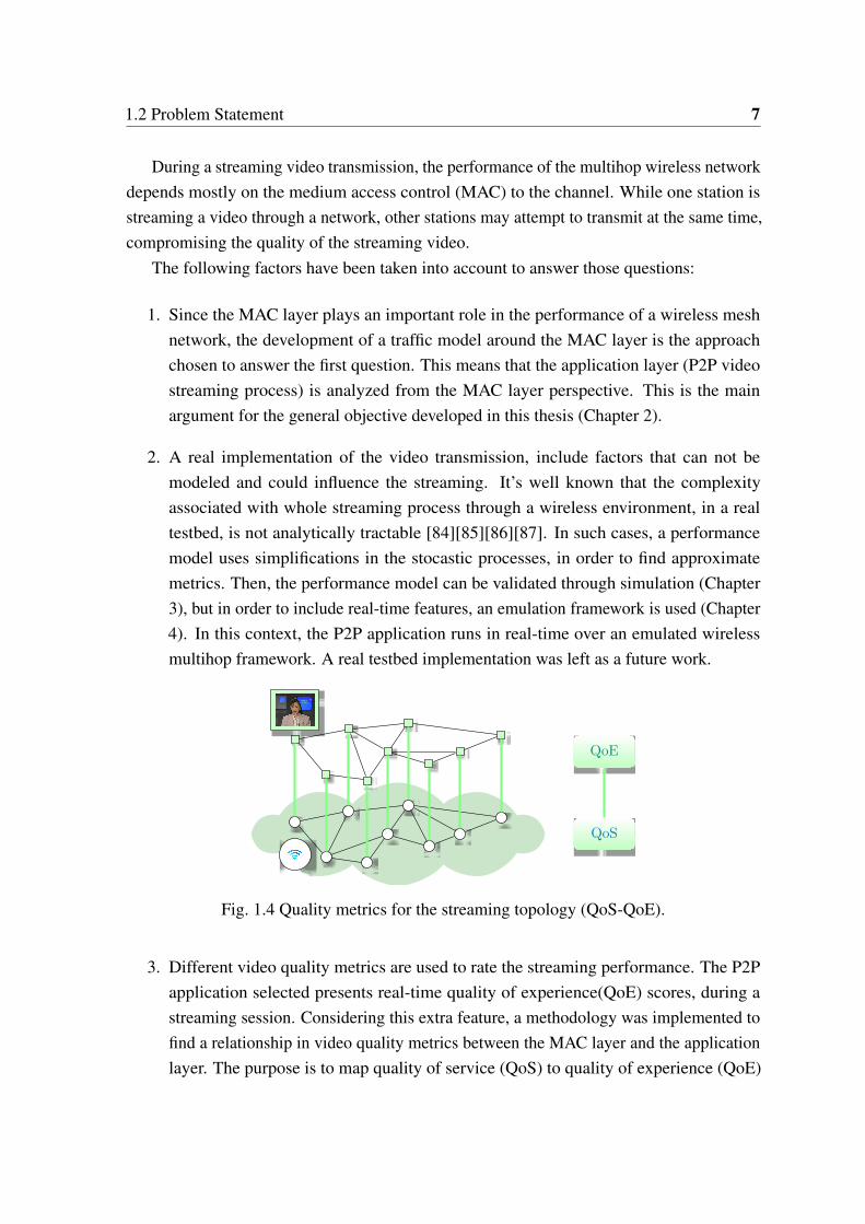
3. Different video quality metrics are used to rate the streaming performance. The P2Papplication selected presents real-time quality of experience(QoE) scores, during astreaming session. Considering this extra feature, a methodology was implemented tofind a relationship in video quality metrics between the MAC layer and the applicationlayer. The purpose is to map quality of service (QoS) to quality of experience (QoE)
8 Introduction
scores (Fig. 1.4). This approach would help to estimate QoE metrics from QoS metrics,obtained from the analytical performance model (Chapter 5).
1.2.1 Objectives
General
• To identify the factors that affect the quality of streaming video in WMN, through thedevelopment of a performance evaluation model.
Specific
• To define the model parameters considering topology, mobility, channel, and commu-nication protocols (Chapter 1).
• To develop a performance evaluation model for the WMN specified (Chapter 2).
• To establish performance metrics considering streaming video for the defined WMN(Chapter 3 and Chapter 4).
• To determine the factors that affect QoS metrics in streaming video on the performancemodel developed for WMN (Chapter 5).
1.3 Thesis structure
This thesis is organized as follows. The chapter 2 introduces state of art of performanceevaluation models, applied to IEEE 802.11 wireless networks. These performance modelsuse different techniques to find the network QoS metrics like throughput, delay and jitter.Then, the proposed performance model for MHWN is formulated including interferenceand topology factors. In chapter 3, the analytical performance model is implemented inPython and validated against a WMN simulation model, available in NS-3. In chapter 4, theperformance of a real P2P video streaming is evaluated using the analytical model defined,and validated through emulation framework, also available in the NS-3 WMN simulationmodel. The chapter 5 presents a statistical analysis including other factors affecting the vidoequality, from the emulated model, and establish a relationship between application layer andMAC layer quality metrics. Chapter 6 consolidates the main contributions of this thesis, andthe list of publications.
Chapter 2
Performance model for IEEE 802.11multihop wireless networks
2.1 Introduction
Performance evaluation of telecommunication systems is an essential topic, due to thewidespread use of these systems in everyday life. Each stage of the system has a performanceand a cost, from the design to the implementation. Even an existing system can be analyzedto improve its performance and meet future demands [88].
Due to the increasing complexity of telecommunication systems, it is important to findeffective tools and techniques to understand the behavior and the performance of existingsystems, and to predict the performance of systems in the design phase. The performance ofsuch systems is evaluated through real-time measurements, simulations, or analytic modelingdepending on the application scenario [89]. If the system is already implemented, itsperformance can be evaluated using the measurement technique. To evaluate the performanceof a system that cannot be measured, e.g., during the design or development phases, it isnecessary to use analytic or simulation modeling in order to predict the performance [88].
In wireless access technologies, the performance modeling is useful finding adequateoperational conditions. In a distributed wireless channel access scheme, like IEEE 802.11[90] wireless local area network (WLAN), the medium is shared among contending nodes,using a set of rules defined in the standard. The main component in the wireless resourceallocation scheme is the medium access control (MAC) layer. The principal function of MACis to coordinate a fair access of multiple stations competing for channel resources.
The process involved in the definition of a successful transmission, can be represented bya stochastic abstraction model. Analytical models based on stochastic processes, have been
10 Performance model for IEEE 802.11 multihop wireless networks
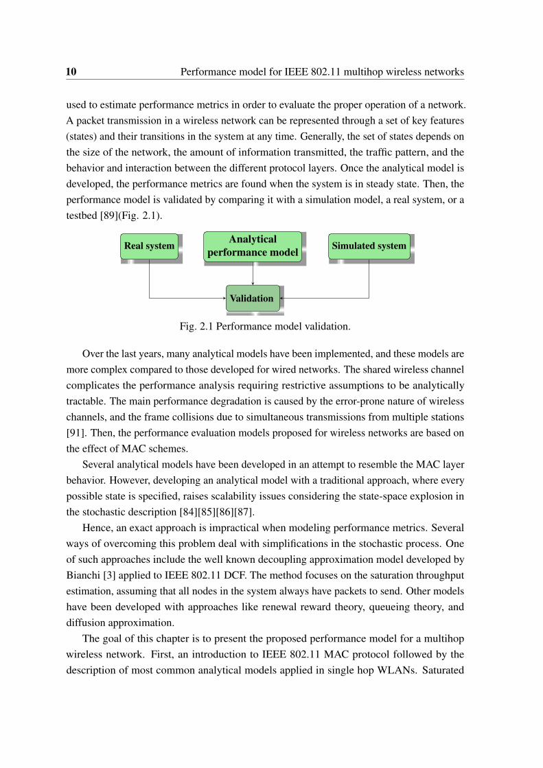
used to estimate performance metrics in order to evaluate the proper operation of a network.A packet transmission in a wireless network can be represented through a set of key features(states) and their transitions in the system at any time. Generally, the set of states depends onthe size of the network, the amount of information transmitted, the traffic pattern, and thebehavior and interaction between the different protocol layers. Once the analytical model isdeveloped, the performance metrics are found when the system is in steady state. Then, theperformance model is validated by comparing it with a simulation model, a real system, or atestbed [89](Fig. 2.1).
Analyticalperformance model Simulated systemReal system
Validation
Fig. 2.1 Performance model validation.
Over the last years, many analytical models have been implemented, and these models aremore complex compared to those developed for wired networks. The shared wireless channelcomplicates the performance analysis requiring restrictive assumptions to be analyticallytractable. The main performance degradation is caused by the error-prone nature of wirelesschannels, and the frame collisions due to simultaneous transmissions from multiple stations[91]. Then, the performance evaluation models proposed for wireless networks are based onthe effect of MAC schemes.
Several analytical models have been developed in an attempt to resemble the MAC layerbehavior. However, developing an analytical model with a traditional approach, where everypossible state is specified, raises scalability issues considering the state-space explosion inthe stochastic description [84][85][86][87].
Hence, an exact approach is impractical when modeling performance metrics. Severalways of overcoming this problem deal with simplifications in the stochastic process. Oneof such approaches include the well known decoupling approximation model developed byBianchi [3] applied to IEEE 802.11 DCF. The method focuses on the saturation throughputestimation, assuming that all nodes in the system always have packets to send. Other modelshave been developed with approaches like renewal reward theory, queueing theory, anddiffusion approximation.
The goal of this chapter is to present the proposed performance model for a multihopwireless network. First, an introduction to IEEE 802.11 MAC protocol followed by thedescription of most common analytical models applied in single hop WLANs. Saturated
2.2 Performance models for distributed wireless access 11
and unsaturated network conditions are considered. Then, the analytical model descriptionsare extended to multihop wireless networks. The last section presents the proposed MHWNperformance model, extending an unsaturated single hop model with topology, interference,queueing and traffic features.
2.2 Performance models for distributed wireless access
In a wireless medium these performance metrics highly depend on how the resource alloca-tion is made. The MAC layer is the principal component in the resolution of informationtransmission through a shared medium, avoiding collisions caused by simultaneous transmis-sions. Most of the performance models are focused on the estimation of quality of service(QoS) metrics like throughput, delay and jitter.
2.2.1 IEEE 802.11 MAC Overview
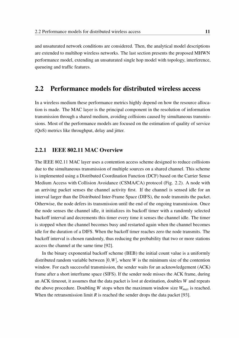
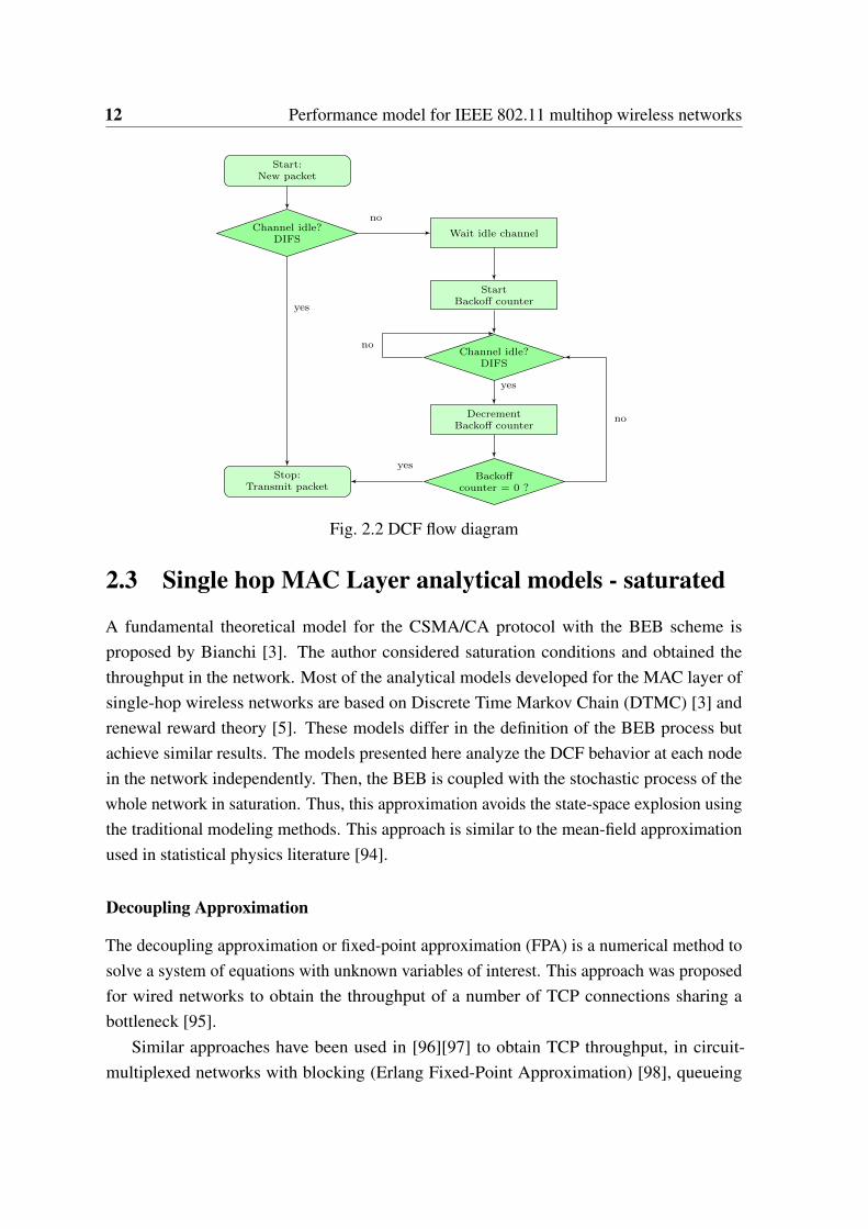
The IEEE 802.11 MAC layer uses a contention access scheme designed to reduce collisionsdue to the simultaneous transmission of multiple sources on a shared channel. This schemeis implemented using a Distributed Coordination Function (DCF) based on the Carrier SenseMedium Access with Collision Avoidance (CSMA/CA) protocol (Fig. 2.2). A node withan arriving packet senses the channel activity first. If the channel is sensed idle for aninterval larger than the Distributed Inter-Frame Space (DIFS), the node transmits the packet.Otherwise, the node defers its transmission until the end of the ongoing transmission. Oncethe node senses the channel idle, it initializes its backoff timer with a randomly selectedbackoff interval and decrements this timer every time it senses the channel idle. The timeris stopped when the channel becomes busy and restarted again when the channel becomesidle for the duration of a DIFS. When the backoff timer reaches zero the node transmits. Thebackoff interval is chosen randomly, thus reducing the probability that two or more stationsaccess the channel at the same time [92].
In the binary exponential backoff scheme (BEB) the initial count value is a uniformlydistributed random variable between [0,W ], where W is the minimum size of the contentionwindow. For each successful transmission, the sender waits for an acknowledgement (ACK)frame after a short interframe space (SIFS). If the sender node misses the ACK frame, duringan ACK timeout, it assumes that the data packet is lost at destination, doubles W and repeatsthe above procedure. Doubling W stops when the maximum window size Wmax is reached.When the retransmission limit R is reached the sender drops the data packet [93].
12 Performance model for IEEE 802.11 multihop wireless networks
Start:New packet
Channel idle?DIFS
Stop:Transmit packet
Wait idle channel
StartBackoff counter
Channel idle?DIFS
DecrementBackoff counter
Backoffcounter = 0 ?
no
yes
yes
no
yes
no
Fig. 2.2 DCF flow diagram
2.3 Single hop MAC Layer analytical models - saturated
A fundamental theoretical model for the CSMA/CA protocol with the BEB scheme isproposed by Bianchi [3]. The author considered saturation conditions and obtained thethroughput in the network. Most of the analytical models developed for the MAC layer ofsingle-hop wireless networks are based on Discrete Time Markov Chain (DTMC) [3] andrenewal reward theory [5]. These models differ in the definition of the BEB process butachieve similar results. The models presented here analyze the DCF behavior at each nodein the network independently. Then, the BEB is coupled with the stochastic process of thewhole network in saturation. Thus, this approximation avoids the state-space explosion usingthe traditional modeling methods. This approach is similar to the mean-field approximationused in statistical physics literature [94].
Decoupling Approximation
The decoupling approximation or fixed-point approximation (FPA) is a numerical method tosolve a system of equations with unknown variables of interest. This approach was proposedfor wired networks to obtain the throughput of a number of TCP connections sharing abottleneck [95].
Similar approaches have been used in [96][97] to obtain TCP throughput, in circuit-multiplexed networks with blocking (Erlang Fixed-Point Approximation) [98], queueing
2.3 Single hop MAC Layer analytical models - saturated 13
networks with time-dependent and state-dependent transition rates (decomposition ap-proach) [99], and non-stationary queueing networks with multi-rate loss queues (fixed-pointapproximation)[100].
2.3.1 Decoupling Approximation in wireless networks
The authors in [101] apply the FPA technique to distinguish between packet losses causedby imperfect error correction at the data-link layer, and packet losses dominated by bufferoverflows. In [102] study the throughput of a single TCP source in wireless and bufferdominated regimes of operation.
The objective of Bianchi’s model [3] is to estimate the throughput of a single-hop wirelessnetwork with n active nodes. The model assumes a single collision domain where only onenode out of n successfully transmits a packet at any time. In this case the FPA consistsin bringing together two equations binding two unknown variables of interest [91]. In thecase of CSMA/CA these variables are the frame collision probability due to simultaneoustransmission attempts performed by two or more stations and the probability that a stationtransmits in an arbitrary slot.
The fundamental principle of the decoupling approximation is that collisions, in a n nodesnetwork, form an i.i.d process for each station. This means that the collision probability isconstant and independent between n stations. This leads to a system of equations relating theper-station attempt rate with the collision probability of a packet. The key approximation isto assume that the aggregate attempt process of the other (n−1) nodes is independent of thebackoff process of the given node [5][3].
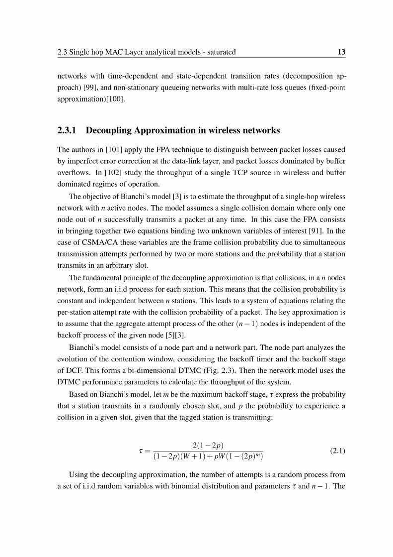
Bianchi’s model consists of a node part and a network part. The node part analyzes theevolution of the contention window, considering the backoff timer and the backoff stageof DCF. This forms a bi-dimensional DTMC (Fig. 2.3). Then the network model uses theDTMC performance parameters to calculate the throughput of the system.
Based on Bianchi’s model, let m be the maximum backoff stage, τ express the probabilitythat a station transmits in a randomly chosen slot, and p the probability to experience acollision in a given slot, given that the tagged station is transmitting:
τ =2(1−2p)
(1−2p)(W +1)+ pW (1− (2p)m)(2.1)
Using the decoupling approximation, the number of attempts is a random process froma set of i.i.d random variables with binomial distribution and parameters τ and n−1. The
14 Performance model for IEEE 802.11 multihop wireless networks
(1 − p)/CW0
p/CWm
0,0
1,0
2,0
· · ·
7,0
0,0
1,0
2,0
· · ·
7,0
· · ·
· · ·
· · ·
· · ·
0,CW0 − 1
1,CW1 − 1
2,CW2 − 1
· · ·
7,CWM−1 − 1
p/CW1
p/CW2
p/CWM
Fig. 2.3 DTMC of Binary Exponential Backoff [3]
conditional collision probability p, is equal to the probability that at least one of the othern−1 stations is accessing the channel.
p = 1− (1− τ)n−1 (2.2)
These equations represent a nonlinear system with two unknowns τ and p. The solutionset of equations system is found using a FPA.
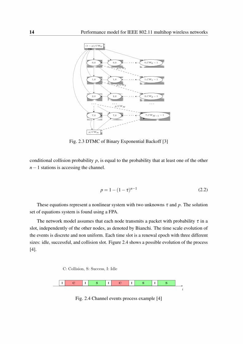
The network model assumes that each node transmits a packet with probability τ in aslot, independently of the other nodes, as denoted by Bianchi. The time scale evolution ofthe events is discrete and non uniform. Each time slot is a renewal epoch with three differentsizes: idle, successful, and collision slot. Figure 2.4 shows a possible evolution of the process[4].
t
C: Collision, S: Success, I: Idle
I C I S I C I S I S
Fig. 2.4 Channel events process example [4]
2.3 Single hop MAC Layer analytical models - saturated 15
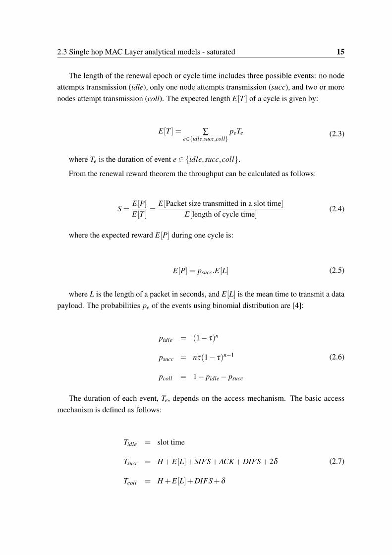
The length of the renewal epoch or cycle time includes three possible events: no nodeattempts transmission (idle), only one node attempts transmission (succ), and two or morenodes attempt transmission (coll). The expected length E[T ] of a cycle is given by:
E[T ] = ∑e∈idle,succ,coll
peTe (2.3)
where Te is the duration of event e ∈ idle,succ,coll.From the renewal reward theorem the throughput can be calculated as follows:
S =E[P]E[T ]
=E[Packet size transmitted in a slot time]
E[length of cycle time](2.4)
where the expected reward E[P] during one cycle is:
E[P] = psucc.E[L] (2.5)
where L is the length of a packet in seconds, and E[L] is the mean time to transmit a datapayload. The probabilities pe of the events using binomial distribution are [4]:
pidle = (1− τ)n
psucc = nτ(1− τ)n−1
pcoll = 1− pidle− psucc
(2.6)
The duration of each event, Te, depends on the access mechanism. The basic accessmechanism is defined as follows:
Tidle = slot time
Tsucc = H +E[L]+SIFS+ACK +DIFS+2δ
Tcoll = H +E[L]+DIFS+δ
(2.7)
16 Performance model for IEEE 802.11 multihop wireless networks
where δ is the propagation delay, H is the time to transmit PHY/MAC headers. Bianchiupdated his original model [103] including the maximum retransmission limit, and addingstates to the original DTMC.
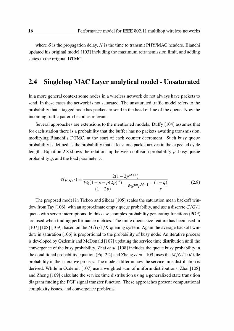
2.4 Singlehop MAC Layer analytical model - Unsaturated
In a more general context some nodes in a wireless network do not always have packets tosend. In these cases the network is not saturated. The unsaturated traffic model refers to theprobability that a tagged node has packets to send in the head of line of the queue. Now theincoming traffic pattern becomes relevant.
Several approaches are extensions to the mentioned models. Duffy [104] assumes thatfor each station there is a probability that the buffer has no packets awaiting transmission,modifying Bianchi’s DTMC, at the start of each counter decrement. Such busy queueprobability is defined as the probability that at least one packet arrives in the expected cyclelength. Equation 2.8 shows the relationship between collision probability p, busy queueprobability q, and the load parameter r.
τ(p,q,r) =2(1−2pM+1)
W0(1− p− p(2p)m)
(1−2p)−W02m pM+1 +
(1−q)r
(2.8)
The proposed model in Tickoo and Sikdar [105] scales the saturation mean backoff win-dow from Tay [106], with an approximate empty queue probability, and use a discrete G/G/1queue with server interruptions. In this case, complex probability generating functions (PGF)are used when finding performance metrics. The finite queue size feature has been used in[107] [108] [109], based on the M/G/1/K queuing system. Again the average backoff win-dow in saturation [106] is proportional to the probability of busy node. An iterative processis developed by Ozdemir and McDonald [107] updating the service time distribution until theconvergence of the busy probability. Zhai et al. [108] includes the queue busy probability inthe conditional probability equation (Eq. 2.2) and Zheng et al. [109] uses the M/G/1/K idleprobability in their iterative process. The models differ in how the service time distribution isderived. While in Ozdemir [107] use a weighted sum of uniform distributions, Zhai [108]and Zheng [109] calculate the service time distribution using a generalized state transitiondiagram finding the PGF signal transfer function. These approaches present computationalcomplexity issues, and convergence problems.
2.5 Performance models in multihop wireless networks 17
In Alizadeh and Subramaniam [110], Bianchi’s DTMC is adapted to non-saturatingtraffic, including the probability of no packet arrival at a given node. The whole network ismodeled as an M/G/1 virtual queue to which packets arrive and receive service from thechannel.
Zhao et al. [111] scales the attempt rate of the saturation mode with the probability ofhaving a packet to transmit. This probability is related to the empty state in a G/G/1 queue.The same authors update their model [93] with an M/G/1/K queue in order to find thewaiting time distribution. The MAC service time distribution is dependent on the collisionprobability, the backoff window and the channel event probabilities. The model presentssimplifications in the queueing process in order to reduce the complexity of the analysis. Ifthe amount of traffic is moderate the model presents multiple solutions in the fixed pointequations.
2.5 Performance models in multihop wireless networks
In a multihop wireless network each node is able to forward packets until they reach des-tination. Typical examples of multihop wireless networks (MHWN) are: wireless sensornetworks (WSN), wireless mesh networks (WMN), and vehicular ad hoc networks (VANET).This class of networks are an active part of the future Internet, like in the development ofsmart cities through the Internet of Things (IoT) [112], and creating intelligent transportationsystems [113].
The implementation of MHWNs faces performance issues, considering various factorssuch as the distance between the nodes, their transmission power, the channel characteristics,and the transmission data rate [114]. Because of the sharing wireless medium conditions, theperformance of the MHWN depends mostly on the control access mechanism (MAC) to thechannel. While one node or station is transmitting packets through a network, other stationsmay attempt to transmit at the same time, compromising the performance of the MHWN.
In order to understand the performance of MHWN and enhance the protocol operation,an analytical model is required to predict and evaluate the performance of MHWN and theirprotocols. Several analytical models have been developed to find performance measures.Throughput, delay and jitter are the main performance metrics, determining quality of service(QoS) within a wireless local area network (WLAN), highly related to the MAC layer. TheIEEE 802.11 MAC layer implements a channel contention access scheme designed to reducecollisions when multiple sources attempt simultaneous transmission.
18 Performance model for IEEE 802.11 multihop wireless networks
2.5.1 Related models
In multihop wireless networks (MHWN), one of the main sources of collisions is the inter-ference associated with both intra-flow and inter-flow transmissions. Performance modelsexposed in this section include different interference models that take into consideration thestation’s position, the hidden terminal problem, transmission range and carrier sense range.
Some authors focus in a random node distribution in the network, like the approach by Xieet al. [115] based on [105], which extends the single-hop model considering a network withuniformly distributed nodes, and determines the number of nodes in two areas based on theircorrespondent transmission range. Nguyen et al. [116] compute the throughput of a givenpath in multihop wireless networks. The authors consider intra-flow interference, hiddennodes and the set of nodes in the transmission range, carrier sense range, and interferencerange. The traffic load is included using the approximation in [117].
Garcia et al. [118] uses an interference matrix based on PHY and MAC layers. The linearsystem has a solution regardless of the network topology. They assume a two-dimensionalPoisson distribution for node locations. The back-off behavior and the channel busy statuswas simplified into a limiting probability.
The model in Abdullah et al. [119] considers random network topology (two-dimensionalPoisson distribution) and the proposed analytical models are verified by simulations withNS-2. The authors implement a collision probability model for hidden terminal problem,considering the intersection of event areas.
Alizadeh and Subramaniam [110], use Bianchi’s DTMC [3] adapted to non-saturatingtraffic, including the probability of no packet arrival at a given node. The whole network ismodeled as a virtual queue (M/G/1) to which packets arrive and receive service from thechannel. The interference range is related to the probability of a source node transmitting anarbitrary packet to a neighboring node, as a function of the traffic and the routing algorithm.However, the total end-to-end delay in multihop networks has not been addressed and onlythe approximate throughput for the multihop condition has been calculated [120][87]. Theyalso assume a pre-backoff algorithm and a pre-knowledge of the neighbors of each node(a predetermined nodes distribution). They concluded that the delay in multihop ad hocnetworks is affected by the hidden-terminals and by the transmission and interference rangeof the wireless devices.
Ghadimi et al. [120] extended the Bianchi’s DTMC in [3] to estimate the end-to-enddelay analysis in MHWN under finite load conditions (unsaturated) considering the hiddenand exposed terminal problem. Each node is represented as an M/G/1 queue, used to computeservice time distribution. The multihop condition is addressed using the events in the hiddenarea of a given node, in an uniform distribution environment. The method used to compute
2.5 Performance models in multihop wireless networks 19
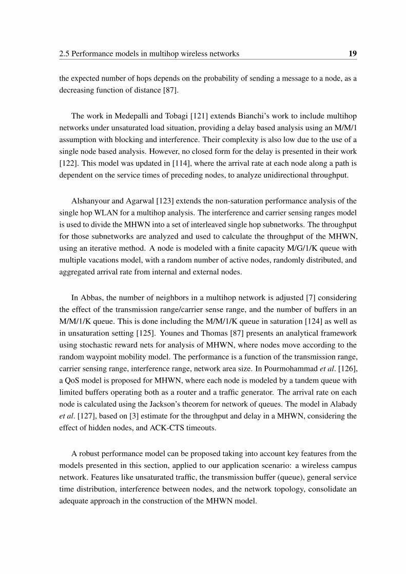
the expected number of hops depends on the probability of sending a message to a node, as adecreasing function of distance [87].
The work in Medepalli and Tobagi [121] extends Bianchi’s work to include multihopnetworks under unsaturated load situation, providing a delay based analysis using an M/M/1assumption with blocking and interference. Their complexity is also low due to the use of asingle node based analysis. However, no closed form for the delay is presented in their work[122]. This model was updated in [114], where the arrival rate at each node along a path isdependent on the service times of preceding nodes, to analyze unidirectional throughput.
Alshanyour and Agarwal [123] extends the non-saturation performance analysis of thesingle hop WLAN for a multihop analysis. The interference and carrier sensing ranges modelis used to divide the MHWN into a set of interleaved single hop subnetworks. The throughputfor those subnetworks are analyzed and used to calculate the throughput of the MHWN,using an iterative method. A node is modeled with a finite capacity M/G/1/K queue withmultiple vacations model, with a random number of active nodes, randomly distributed, andaggregated arrival rate from internal and external nodes.
In Abbas, the number of neighbors in a multihop network is adjusted [7] consideringthe effect of the transmission range/carrier sense range, and the number of buffers in anM/M/1/K queue. This is done including the M/M/1/K queue in saturation [124] as well asin unsaturation setting [125]. Younes and Thomas [87] presents an analytical frameworkusing stochastic reward nets for analysis of MHWN, where nodes move according to therandom waypoint mobility model. The performance is a function of the transmission range,carrier sensing range, interference range, network area size. In Pourmohammad et al. [126],a QoS model is proposed for MHWN, where each node is modeled by a tandem queue withlimited buffers operating both as a router and a traffic generator. The arrival rate on eachnode is calculated using the Jackson’s theorem for network of queues. The model in Alabadyet al. [127], based on [3] estimate for the throughput and delay in a MHWN, considering theeffect of hidden nodes, and ACK-CTS timeouts.
A robust performance model can be proposed taking into account key features from themodels presented in this section, applied to our application scenario: a wireless campusnetwork. Features like unsaturated traffic, the transmission buffer (queue), general servicetime distribution, interference between nodes, and the network topology, consolidate anadequate approach in the construction of the MHWN model.

20 Performance model for IEEE 802.11 multihop wireless networks
2.6 Background for the proposed MHWN model
The following single hop wireless model is the base of the multihop model proposed insection 2.7.1.
2.6.1 Singlehop MAC Layer analytical model
This section describes the unsaturated single-hop MAC model developed by Zhao et al. [93],an extension of Kumar’s model [5].
Analysis of the backoff process
Successes
Collisions
R1 = 2
B01 B1
1
X1
R2 = 4
B02 B1
2 B22 B3
2
X2
R3 = 2
B03 B1
3
X3
R4 = 1
B04
X4
Fig. 2.5 Evolution of the back-offs of a node. Each attempted packet starts a new back-offcycle [5].
Let γ denote the collision probability on the condition that the buffer is not empty. R j
represents the number of attempts until success for the jth packet. Each unsuccessful attemptgenerates a new backoff sequence, so the total backoff time is proportional to the number ofattempts. This time is represented through the sum of weighted discrete uniform distributionsX j [5]. The sequence X j can be seen as a renewal life time. In this case the number ofattempts R j can be considered as a reward in the renewal cycle of length X j.
Let βc denote the attempt rate per slot on the condition that the buffer is not empty [5, 93],representing the proportion between the number of attempts and the backoff time :
βc(γ) =1+ γ + γ2 + · · ·+ γM−1
b0 + γb1 + γ2b2 + · · ·+ γM−1bM−1
βc(γ) = R/X
(2.9)
where R represents the number of attempts until success for a packet, with the attemptlimit M. R is modeled as a truncated geometric random variable with parameter 1− γ . Thetotal backoff time (X) is proportional to the number of attempts, and is represented throughthe sum of weighted discrete uniform distribution, where bk is the mean backoff time of
2.6 Background for the proposed MHWN model 21
stage k for each node [5]. The sequence X can be seen as a renewal life time. In this case thenumber of attempts R can be considered as a reward in the renewal cycle of length X .
Now, using the decoupling approximation, the number of attempts made by the othernodes is binomially distributed with parameters β and n− 1. The conditional collisionprobability γ , is equivalent to the probability that at least one of the other n− 1 stationsattempt to transmit:
γ = 1− (1−βc(γ))n−1 (2.10)
Equations (2.6.1) and (2.10) represent a nonlinear system with two unknowns τ and p. Thesolution set of the system of equations is found using a fixed point approximation. Thissolution is the saturation collision probability γs, and the saturation attempt rate βs.
2.6.2 Unsaturated MAC Service Time
The unsaturated traffic case is modeled proportional to the attempt rate of the saturated caseincluding the probability of a nonempty buffer. The following equations are presented by[93]. Let p0 be the probability of an empty buffer, and let β be the general attempt rateproportional to system utilization (1− p0) and the conditional attempt rate [93]:
β = (1− p0)βc (2.11)
γ(β ) = 1− (1−β )n−1 (2.12)
In this case γ is the general collision probability. The variable p0 is related to the trafficintensity ρ . The system utilization ρ is related to the service time Yc, and the Poisson arrivalprocess with parameter λ , as follows:
ρ(γ) = λYc(γ) (2.13)
where Yc is the service time (in number of slots) of a packet of a tagged node, on the conditionthat the buffer is not empty, as a function of γ and βc. The parameter λ is the arrival packetrate per slot. As seen before, X is a random variable representing the backoff count (measuredin decrements of the backoff counter) that elapses before a packet transmission of the taggednode is finished. Let Ω be a random variable representing the time (in slots) for one decrementof the backoff counter. Since each backoff decrements observe a backoff count of X before
22 Performance model for IEEE 802.11 multihop wireless networks
its packet transmission finishes, Yc is given by [93]:
Yc =X
∑i=1
Ω (2.14)
The random variable X is equal to the sum of the total backoff count spent by the taggednode in different possible subsets of the M backoff stages, and the probability of each subsetcan be expressed in terms of γ [93]:
X =j
∑k=0
ηk,w.p. δ (γ, j),0≤ j ≤M−1,
where δ (γ, j) =
(1− γ)γ j, 0≤ j ≤M−2
γM−1, j = M−1
(2.15)
X = b0 + γgb1 + γ2g b2 + · · ·+ γM−1
g bM−1 (2.16)
where ηk is uniformly distributed in [0,CWk−1] with mean bk, CWk = 2kCW0, and CW0 isthe minimum window size. δ (γ, j) is the probability that the packet transmission finishes atthe jth backoff stage (the same as R j defined above). Then, the probability distribution ofX is the convolution of weighted contention windows ηk, with weights δ (γ). The equation2.16 is the average of the sum of the total backoff count X . Each slot duration Ω depends onwhether a slot is idle, a successful transmission, or a collision [93]:
Ω =
σ , w.p. 1−Pb,
Ts +σ , w.p. Ps,
Ts +σ , w.p. Ps,
(2.17)
Pb = 1− (1−βc)n = 1− (1− γ)
nn−1
Ps = nβc(1−βc)n−1 = n(1− (1− γ)
1n−1 )(1− γ)
Ps = Pb−Ps
(2.18)
where Pb is the probability of a busy slot, Ps is the probability of successful transmissionfrom any of the n contending nodes, and Ps is the probability of a collision from any of the
2.6 Background for the proposed MHWN model 23
n contending nodes; Ts and Ts are the mean time in slots for successful and unsuccessfultransmission, respectively, and depend on the packet payload and the protocol parameters(σ = 1 slot). Then, the average of the time for one decrement of the backoff counter Ω is:
Ω = σ +PsTs +PsTs (2.19)
2.6.3 Sensitivity analysis
The general fixed point expressed in Eq. 2.12, is an increasing function with respect toβ since β ≤ βc, then the general collision probability is less than the saturated collisionprobability (γ ≤ γs). In [5] the authors show the convergence of the fixed point method yieldsto a unique solution, for the saturated case. For the unsaturated case, the authors in [6] provethe convergence and the uniqueness of the general fixed point equations 2.12 and 2.11.
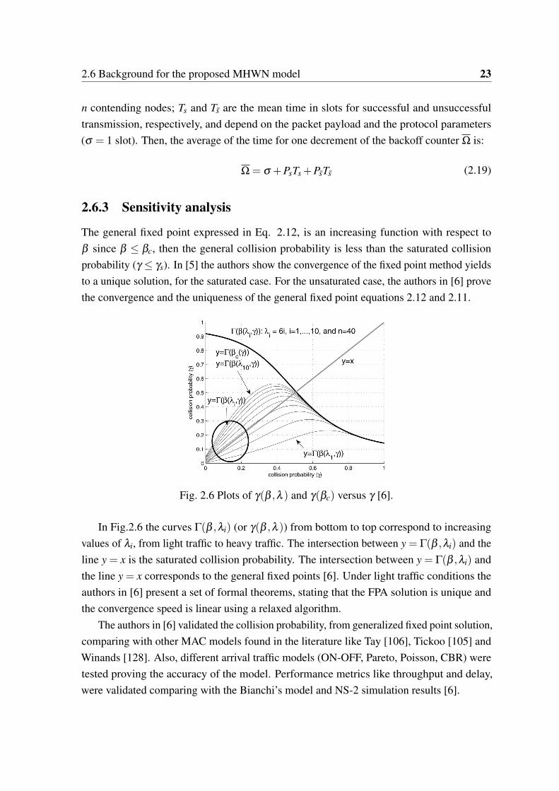
Fig. 2.6 Plots of γ(β ,λ ) and γ(βc) versus γ [6].
In Fig.2.6 the curves Γ(β ,λi) (or γ(β ,λ )) from bottom to top correspond to increasingvalues of λi, from light traffic to heavy traffic. The intersection between y = Γ(β ,λi) and theline y = x is the saturated collision probability. The intersection between y = Γ(β ,λi) andthe line y = x corresponds to the general fixed points [6]. Under light traffic conditions theauthors in [6] present a set of formal theorems, stating that the FPA solution is unique andthe convergence speed is linear using a relaxed algorithm.
The authors in [6] validated the collision probability, from generalized fixed point solution,comparing with other MAC models found in the literature like Tay [106], Tickoo [105] andWinands [128]. Also, different arrival traffic models (ON-OFF, Pareto, Poisson, CBR) weretested proving the accuracy of the model. Performance metrics like throughput and delay,were validated comparing with the Bianchi’s model and NS-2 simulation results [6].
24 Performance model for IEEE 802.11 multihop wireless networks
2.6.4 M/G/1 queuing model
The system utilization ρ is used to find p0 applying the method developed in [129] and [130].In an M/G/1 analysis, let πM/G/1 be the steady state probability of the queue. Then, theprobability generating function (PGF) of πM/G/1(λ ) is:
πM/G/1(λ ,z) =(1−ρ(γ))(1− z)Yc(γ,e−(1−z)λ )
Yc(γ,e−(1−z)λ )− z(2.20)
where Yc(γ,z) is the PGF of the service time random variable.
2.6.5 MAC Service time distribution
From Eq. 2.14 the PGF of the MAC service time distribution Yc is a compound function,depending on the PGF of X and the PGF Ω [131]:
Yc(γ,z) = X(γ,Ω(γ,z)) (2.21)
Considering the PGF of the contention windows ηk:
η(z) =
1
CWk
1− zCWk
1− z, 0 < k < m,
1CWm
1− zCWm
1− z, m < k < M−1
(2.22)
the respective PGFs of X (Eq 2.15) and Ω (Eq. 2.17), are defined as:
X =M−1
∑i=0
[δ (γ, i)
i
∏k=0
η(z)
](2.23)
Ω = (1−Pb)zσ +PszTs+σ +PszTs+σ (2.24)
The average of the service time distribution Yc is the product of the average of the sum of thetotal backoff count X and the average of the time for one decrement of the backoff counter Ω:
Yc = X(γ) ·Ω(γ) (2.25)
2.7 Proposed performance model for MHWN 25
2.6.6 Throughput
From the renewal reward theorem the throughput can be calculated as follows [3]:
S =E[Packet duration transmitted in a slot time]
E[slot event duration]
S =Ps.E[L]
Ω(2.26)
where E[L] is the mean time in slots needed to transmit a data payload.
2.6.7 Delay distribution
Let D be the sojourn time of a packet in the M/G/1 transmit buffer. The Laplace transform ofthe delay distribution is given by: [89]:
DM/G/1(s) =s(1−ρ)Yc(γ,e−s)
s−λ (1− Yc(γ,e−s))(2.27)
and the waiting time for an M/G/1 queue:
WM/G/1(s) =s(1−ρ)
s−λ (1− Yc(γ,e−s))(2.28)
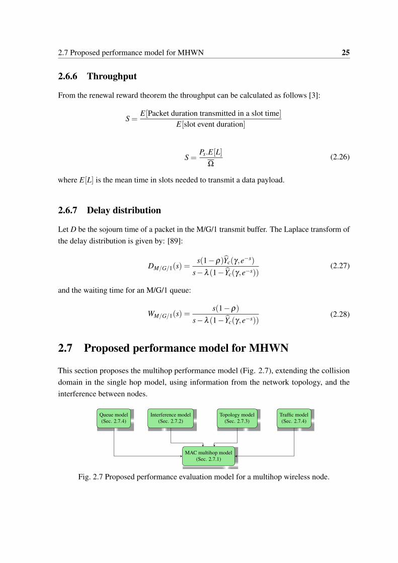
2.7 Proposed performance model for MHWN
This section proposes the multihop performance model (Fig. 2.7), extending the collisiondomain in the single hop model, using information from the network topology, and theinterference between nodes.
Queue model(Sec. 2.7.4)
Interference model(Sec. 2.7.2)
Topology model(Sec. 2.7.3)
Traffic model(Sec. 2.7.4)
MAC multihop model(Sec. 2.7.1)
Fig. 2.7 Proposed performance evaluation model for a multihop wireless node.
26 Performance model for IEEE 802.11 multihop wireless networks
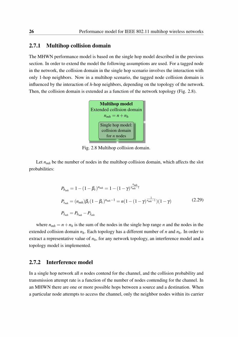
2.7.1 Multihop collision domain
The MHWN performance model is based on the single hop model described in the previoussection. In order to extend the model the following assumptions are used. For a tagged nodein the network, the collision domain in the single hop scenario involves the interaction withonly 1-hop neighbors. Now in a multihop scenario, the tagged node collision domain isinfluenced by the interaction of h-hop neighbors, depending on the topology of the network.Then, the collision domain is extended as a function of the network topology (Fig. 2.8).
Multihop modelExtended collision domain
nmh = n+nh
Single hop model:collision domain
for n nodes
Fig. 2.8 Multihop collision domain.
Let nmh be the number of nodes in the multihop collision domain, which affects the slotprobabilities:
Pbmh = 1− (1−βc)nmh = 1− (1− γ)
nmhnmh−1
Psmh = (nmh)βc(1−βc)nmh−1 = n(1− (1− γ)
1nmh−1 )(1− γ)
Psmh = Pbmh−Psmh
(2.29)
where nmh = n+nh is the sum of the nodes in the single hop range n and the nodes in theextended collision domain nh. Each topology has a different number of n and nh. In order toextract a representative value of nh, for any network topology, an interference model and atopology model is implemented.
2.7.2 Interference model
In a single hop network all n nodes contend for the channel, and the collision probability andtransmission attempt rate is a function of the number of nodes contending for the channel. Inan MHWN there are one or more possible hops between a source and a destination. Whena particular node attempts to access the channel, only the neighbor nodes within its carrier
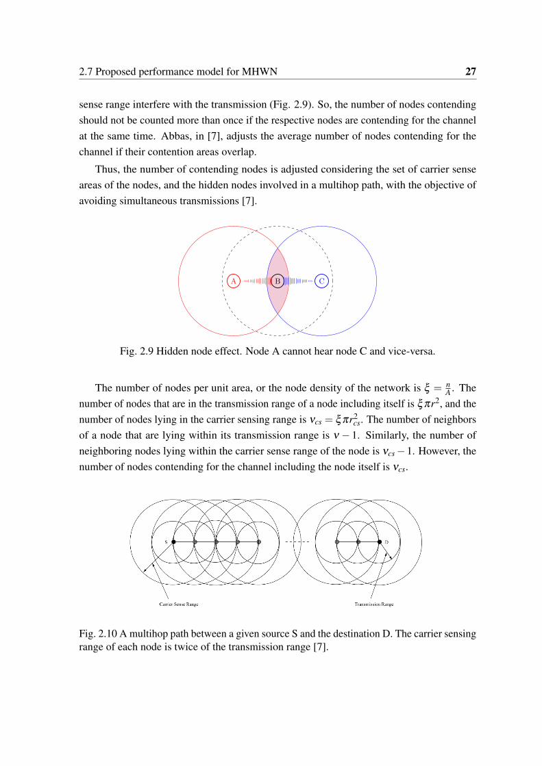
2.7 Proposed performance model for MHWN 27
sense range interfere with the transmission (Fig. 2.9). So, the number of nodes contendingshould not be counted more than once if the respective nodes are contending for the channelat the same time. Abbas, in [7], adjusts the average number of nodes contending for thechannel if their contention areas overlap.
Thus, the number of contending nodes is adjusted considering the set of carrier senseareas of the nodes, and the hidden nodes involved in a multihop path, with the objective ofavoiding simultaneous transmissions [7].
A B C
Fig. 2.9 Hidden node effect. Node A cannot hear node C and vice-versa.
The number of nodes per unit area, or the node density of the network is ξ = nA . The
number of nodes that are in the transmission range of a node including itself is ξ πr2, and thenumber of nodes lying in the carrier sensing range is νcs = ξ πr2
cs. The number of neighborsof a node that are lying within its transmission range is ν − 1. Similarly, the number ofneighboring nodes lying within the carrier sense range of the node is νcs−1. However, thenumber of nodes contending for the channel including the node itself is νcs.
Fig. 2.10 A multihop path between a given source S and the destination D. The carrier sensingrange of each node is twice of the transmission range [7].

28 Performance model for IEEE 802.11 multihop wireless networks
Common area between two nodes
The common area between two circles of the same radii R, and whose centers are separatedby a distance t, is expressed as [119]:
A(t,R) = 2R2
arccos( t
2R
)− t
4R2 (4R2− t2)12
(2.30)
Fig. 2.11 Common area between the carrier sense ranges of two adjacent nodes with adistance between their centers t = r [7].
For S and the first intermediate node, t = rcs2 , R = rcs :
AS,i1 = 2.1521r2cs
a1 ≈ 2r2cs
13π
31−√
1516
(2.31)
where a1 is the area that is common between node i and j, in 1 hop.
Common area among the nodes lying along a path
In the case of two nodes along a path, let c1 and c2 be contention area of a node 1 and tworespectively. The common area along the nodes is:
2.7 Proposed performance model for MHWN 29
c1∪ c2 = c1 + c2− c1∩ c2
= a+a−a1 = 2a−a1(2.32)
Considering the relationship between common areas a1, and the sum of the areas 2a, theadjustment factor for two nodes is:
χ =a1
2a
=2.1521r2
cs2πr2
cs
=2.1521
2π
=2.1521
π
(1− 1
2
)(2.33)
For n nodes along a path, let ci be contention area of a node i. The contention area of asingle node is a = πr2
cs. The contention area that is common among a set of h nodes along apath is given by the addition rule in set theory [7]:
⋃hl=1 cl = ∑
hi=1 ci−∑
i= j=hi, j=1,i= j ci∩ c j
+∑i= j=k=hi, j,k=1,i= j =k ci∩ c j∩ ck− ·· · +(−1)h+1 c1∩·· ·∩ ch.
(2.34)
Adjustment for the number of contending nodes
Let h be the number of nodes along a path from a given source to a destination, and let N′cs
be the adjusted average number of neighbors lying in the carrier sense range of a node alongthe path, represented by [7]:
N′cs = Ncs(1−χ) (2.35)

30 Performance model for IEEE 802.11 multihop wireless networks
Using induction, an expression for the unions of the contention areas of single, two, three,through n nodes, the adjustment factor gives [7]:
χ =2.1521
π
(1− 1
h
)(2.36)
This adjustment factor is used in the performance model to calculate the variable nh statedbefore. Then, a hop count measure is required in order to obtain the number of adjustednodes, in the extended collision domain as expressed in equation 2.37.
χmh =2.1521
π
(1− 1
Average hop count
)(2.37)
Now, expressing Eq. 2.35 in terms of the performance model:
nh = n(1−χmh) (2.38)
The average or mean hop count (HC) value can be extracted from the wireless networktopology using a graph model.
2.7.3 Graph model
A graph G = (V,E) is a pair of sets V vertices (or nodes) and E edges (or arcs), where theedges join pairs of vertices. A graph is a mathematical concept that captures the notion ofconnection [132]. Two vertices are said to be adjacent if they are joined by an edge. If anedge exists between two nodes, the two nodes are neighbors.
1 2 3
4 5 6
7 8 9
10 11 12
Fig. 2.12 Possible application scenario topology for a wireless campus network.
2.7 Proposed performance model for MHWN 31
The graph model abstract the wireless network topology with n nodes, their position (thevertices), and the neighbors of each node connected through a wireless link (the arcs). Thenode positions and their possible links, or connectivity, with other nodes can be representedin matrix notation. Another way to describe a graph is in terms of the adjacency matrix A[ai j],where ai j = 1 if there is a link from i to j (i and j are neighbors), otherwise ai j = 0, for alli, j ∈V [133].
Now, using the assumptions considered in the application scenario (in section 1.1.3), theselected network topology is a regular square grid, where each node has connectivity with itsfour closest neighbors, depending on the distance between nodes (Fig. 2.12). This topologyresembles a possible multihop wireless campus network, where nodes are placed in buildings,halls or squares. This topology can be modeled with an undirected graph G = (V,E) in orderto locate the nodes and links, according to the connectivity or adjacency matrix.
The graph model is useful in finding the average hop count, required in the interferencemodel to calculate nh, defined as the inverse the mean closeness centrality (reciprocal of theshortest path distances from a node to all other nodes).
Closeness centrality
The closeness centrality is the average distance of a node to the other nodes in the network.Let h(s,d) be the shortest path between s and d, or the minimum number of edges (hops)that can be traversed along some path in the network to connect s and d [134][135]. Thecloseness of node s to other nodes in the network is defined as the reciprocal of the sum ofthe distances or hops h(s,d) [136][134][135]:
CCs =1
∑s∈V,s =d∈V
h(s,d) (2.39)
The the average or mean hop count, HC, is the inverse of the mean closeness centralityCC:
Mean hop count(HC) =1
CC(2.40)
High closeness centrality scores indicate that a node can reach other nodes on short pathsor hops [135]. Then nh (Eq. 2.37) is expressed as:
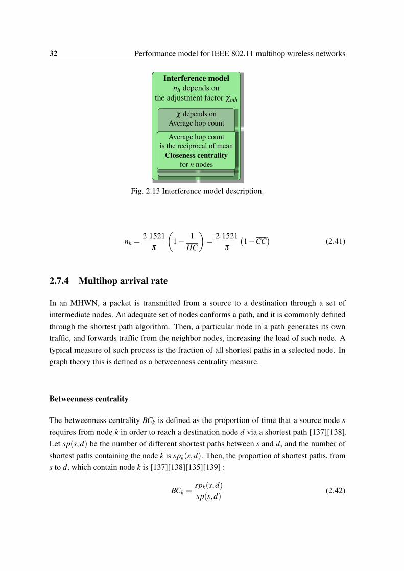
32 Performance model for IEEE 802.11 multihop wireless networks
Interference modelnh depends on
the adjustment factor χmh
χ depends onAverage hop count
Average hop countis the reciprocal of mean
Closeness centralityfor n nodes
Fig. 2.13 Interference model description.
nh =2.1521
π
(1− 1
HC
)=
2.1521π
(1−CC
)(2.41)
2.7.4 Multihop arrival rate
In an MHWN, a packet is transmitted from a source to a destination through a set ofintermediate nodes. An adequate set of nodes conforms a path, and it is commonly definedthrough the shortest path algorithm. Then, a particular node in a path generates its owntraffic, and forwards traffic from the neighbor nodes, increasing the load of such node. Atypical measure of such process is the fraction of all shortest paths in a selected node. Ingraph theory this is defined as a betweenness centrality measure.
Betweenness centrality
The betweenness centrality BCk is defined as the proportion of time that a source node srequires from node k in order to reach a destination node d via a shortest path [137][138].Let sp(s,d) be the number of different shortest paths between s and d, and the number ofshortest paths containing the node k is spk(s,d). Then, the proportion of shortest paths, froms to d, which contain node k is [137][138][135][139] :
BCk =spk(s,d)sp(s,d)
(2.42)
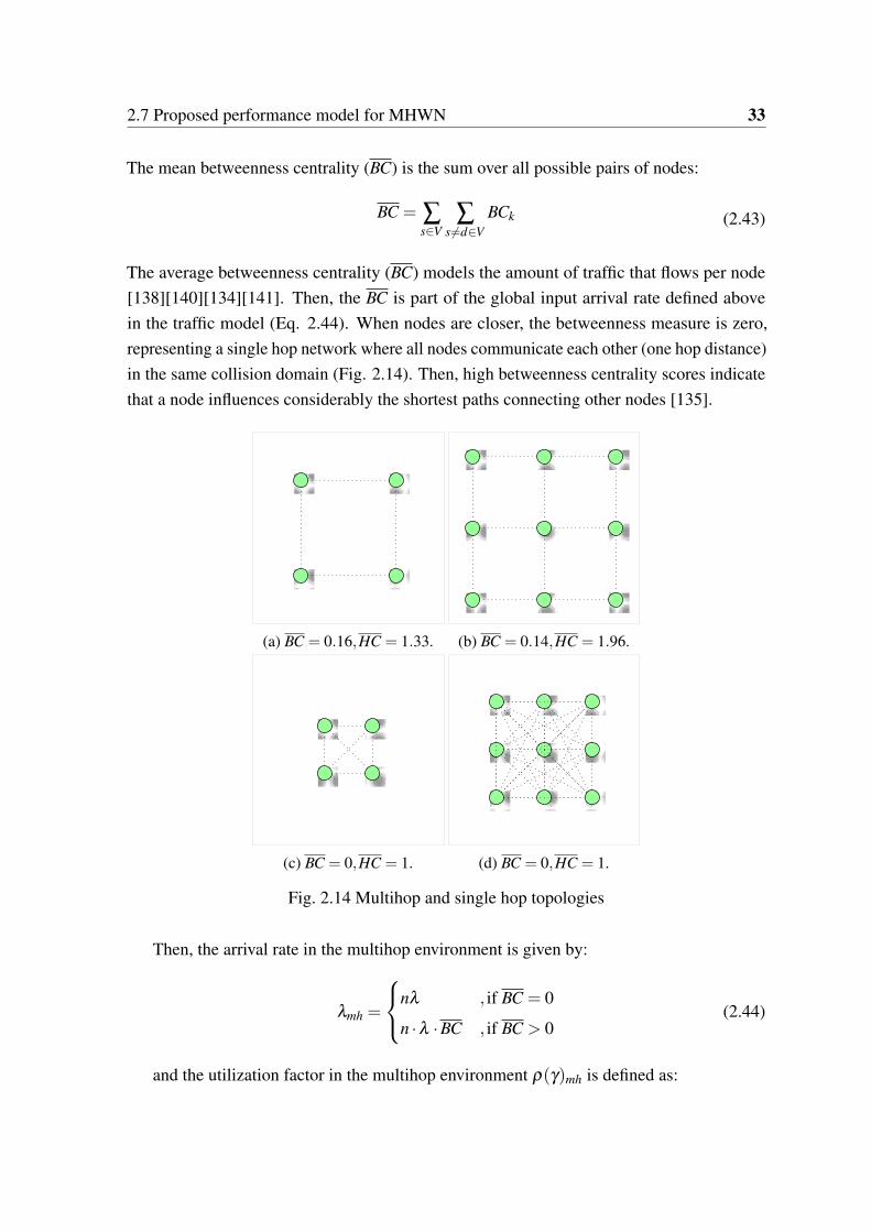
2.7 Proposed performance model for MHWN 33
The mean betweenness centrality (BC) is the sum over all possible pairs of nodes:
BC = ∑s∈V
∑s =d∈V
BCk (2.43)
The average betweenness centrality (BC) models the amount of traffic that flows per node[138][140][134][141]. Then, the BC is part of the global input arrival rate defined abovein the traffic model (Eq. 2.44). When nodes are closer, the betweenness measure is zero,representing a single hop network where all nodes communicate each other (one hop distance)in the same collision domain (Fig. 2.14). Then, high betweenness centrality scores indicatethat a node influences considerably the shortest paths connecting other nodes [135].
(a) BC = 0.16,HC = 1.33. (b) BC = 0.14,HC = 1.96.
(c) BC = 0,HC = 1. (d) BC = 0,HC = 1.
Fig. 2.14 Multihop and single hop topologies
Then, the arrival rate in the multihop environment is given by:
λmh =
nλ , if BC = 0
n ·λ ·BC , if BC > 0(2.44)
and the utilization factor in the multihop environment ρ(γ)mh is defined as:
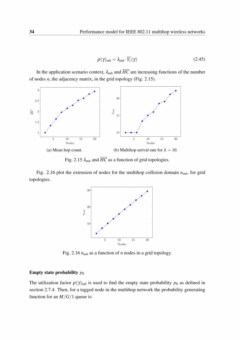
34 Performance model for IEEE 802.11 multihop wireless networks
ρ(γ)mh = λmh ·Yc(γ) (2.45)
In the application scenario context, λmh and HC are increasing functions of the numberof nodes n, the adjacency matrix, in the grid topology (Fig. 2.15).
5 10 15 20
1
1.5
2
2.5
3
Nodes
HC
(a) Mean hop count.
5 10 15 20
10
15
20
Nodes
λm
h
(b) Multihop arrival rate for λ = 10.
Fig. 2.15 λmh and HC as a function of grid topologies.
Fig. 2.16 plot the extension of nodes for the multihop collision domain nmh, for gridtopologies.
5 10 15 20
10
20
30
Nodes
nm
h
Fig. 2.16 nmh as a function of n nodes in a grid topology.
Empty state probability p0
The utilization factor ρ(γ)mh is used to find the empty state probability p0 as defined insection 2.7.4. Then, for a tagged node in the multihop network the probability generatingfunction for an M/G/1 queue is:
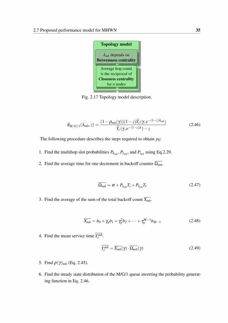
2.7 Proposed performance model for MHWN 35
Topology model
λmh depends onBetwenness centrality
Average hop countis the reciprocal of
Closeness centralityfor n nodes
Fig. 2.17 Topology model description.
πM/G/1(λmh,z) =(1−ρmh(γ))(1− z)Yc(γ,e−(1−z)λmh)
Yc(γ,e−(1−z)λ )− z(2.46)
The following procedure describes the steps required to obtain p0:
1. Find the multihop slot probabilities Pbmh , Psmh , and Pimh using Eq.2.29.
2. Find the average time for one decrement in backoff counter Ωmh.
Ωmh = σ +PsmhTs +PsmhTs (2.47)
3. Find the average of the sum of the total backoff count Xmh.
Xmh = b0 + γgb1 + γ2g b2 + · · ·+ γM−1
g bM−1 (2.48)
4. Find the mean service time Y mhc .
Y mhc = Xmh(γ) ·Ωmh(γ) (2.49)
5. Find ρ(γ)mh (Eq. 2.45).
6. Find the steady state distribution of the M/G/1 queue inverting the probability generat-ing function in Eq. 2.46.

36 Performance model for IEEE 802.11 multihop wireless networks
Service time distribution
The M/G/1 queue PGF, πM/G/1(λmh,z), requires the construction of the service time PGFY mh
c (γmh,z), using the following steps:
1. Find δ (γ, j), the probability that the packet transmission finishes at the j-th backoffstage.
δ (γ, j) =
(1− γmh)γ
jmh, 0≤ j ≤M−2
γM−1mh , j = M−1
(2.50)
2. Find η(z), the PGF of backoff stage η j.
η(z) =
1
CWk
1− zCWk
1− z, 0 < k < m
1CWm
1− zCWm
1− z, m < k < M−1
(2.51)
3. Find Xmh(z), the PGF of sum of the total backoff count X(η ,δ (γmh)) in M backoffstages η with probability δ (γmh).
Xmh =M−1
∑i=0
[δ (γmh, i)
i
∏k=0
η(z)
](2.52)
4. Find Ωmh(z), the PGF of the time for one decrement of the backoff counter.
Ωmh = (1−Pbmh)zσ +PsmhzTs+σ +PsmhzTs+σ (2.53)
5. Find Y mhc (γ,z), the PGF of service time distribution Y mh
c .
Y mhc (γmh,z) = X(γmh,Ωmh(γmh,z)) (2.54)
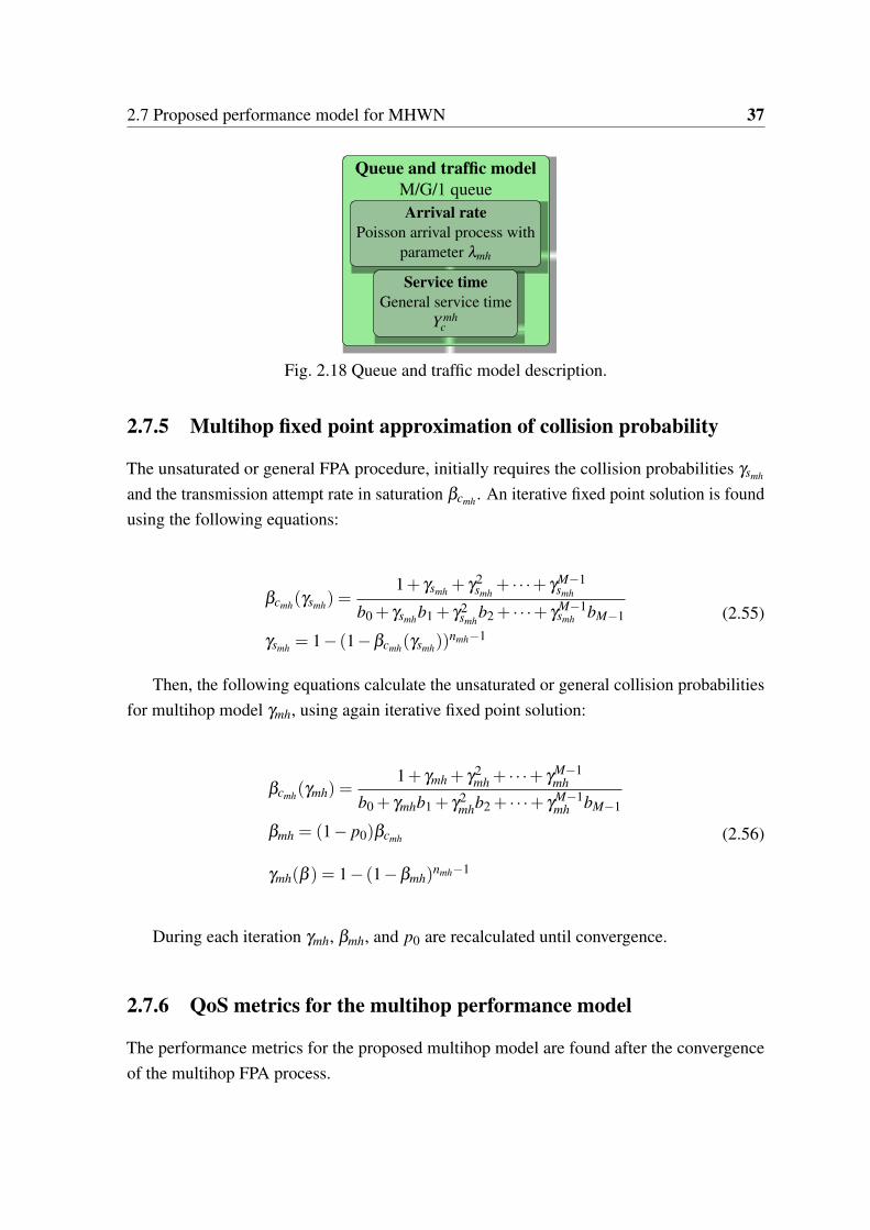
2.7 Proposed performance model for MHWN 37
Queue and traffic modelM/G/1 queueArrival rate
Poisson arrival process withparameter λmh
Service timeGeneral service time
Y mhc
Fig. 2.18 Queue and traffic model description.
2.7.5 Multihop fixed point approximation of collision probability
The unsaturated or general FPA procedure, initially requires the collision probabilities γsmh
and the transmission attempt rate in saturation βcmh . An iterative fixed point solution is foundusing the following equations:
βcmh(γsmh) =1+ γsmh + γ2
smh+ · · ·+ γM−1
smh
b0 + γsmhb1 + γ2smh
b2 + · · ·+ γM−1smh bM−1
γsmh = 1− (1−βcmh(γsmh))nmh−1
(2.55)
Then, the following equations calculate the unsaturated or general collision probabilitiesfor multihop model γmh, using again iterative fixed point solution:
βcmh(γmh) =1+ γmh + γ2
mh + · · ·+ γM−1mh
b0 + γmhb1 + γ2mhb2 + · · ·+ γ
M−1mh bM−1
βmh = (1− p0)βcmh
γmh(β ) = 1− (1−βmh)nmh−1
(2.56)
During each iteration γmh, βmh, and p0 are recalculated until convergence.
2.7.6 QoS metrics for the multihop performance model
The performance metrics for the proposed multihop model are found after the convergenceof the multihop FPA process.
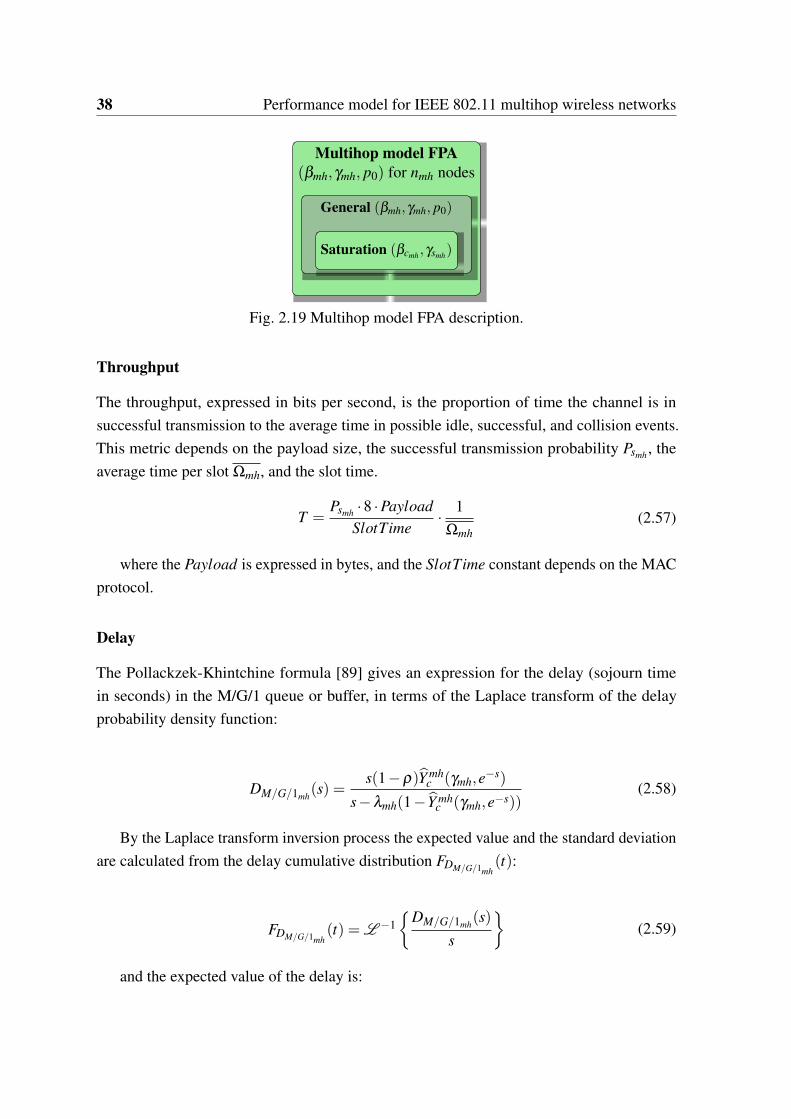
38 Performance model for IEEE 802.11 multihop wireless networks
Multihop model FPA(βmh,γmh, p0) for nmh nodes
General (βmh,γmh, p0)
Saturation (βcmh ,γsmh)
Fig. 2.19 Multihop model FPA description.
Throughput
The throughput, expressed in bits per second, is the proportion of time the channel is insuccessful transmission to the average time in possible idle, successful, and collision events.This metric depends on the payload size, the successful transmission probability Psmh , theaverage time per slot Ωmh, and the slot time.
T =Psmh ·8 ·Payload
SlotTime· 1
Ωmh(2.57)
where the Payload is expressed in bytes, and the SlotTime constant depends on the MACprotocol.
Delay
The Pollackzek-Khintchine formula [89] gives an expression for the delay (sojourn timein seconds) in the M/G/1 queue or buffer, in terms of the Laplace transform of the delayprobability density function:
DM/G/1mh(s) =
s(1−ρ)Y mhc (γmh,e−s)
s−λmh(1− Y mhc (γmh,e−s))
(2.58)
By the Laplace transform inversion process the expected value and the standard deviationare calculated from the delay cumulative distribution FDM/G/1mh
(t):
FDM/G/1mh(t) = L −1
DM/G/1mh
(s)s
(2.59)
and the expected value of the delay is:
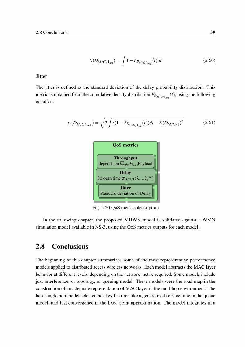
2.8 Conclusions 39
E(DM/G/1mh) =
∫1−FDM/G/1mh
(t)dt (2.60)
Jitter
The jitter is defined as the standard deviation of the delay probability distribution. Thismetric is obtained from the cumulative density distribution FDM/G/1mh
(t), using the followingequation.
σ(DM/G/1mh) =
√2∫
t(1−FDM/G/1mh(t))dt−E(DM/G/1)
2 (2.61)
QoS metrics
Throughputdepends on Ωmh,PSmh ,Payload
DelaySojourn time πM/G/1(λmh,Y mh
c )
JitterStandard deviation of Delay
Fig. 2.20 QoS metrics description
In the following chapter, the proposed MHWN model is validated against a WMNsimulation model available in NS-3, using the QoS metrics outputs for each model.
2.8 Conclusions
The beginning of this chapter summarizes some of the most representative performancemodels applied to distributed access wireless networks. Each model abstracts the MAC layerbehavior at different levels, depending on the network metric required. Some models includejust interference, or topology, or queuing model. These models were the road map in theconstruction of an adequate representation of MAC layer in the multihop environment. Thebase single hop model selected has key features like a generalized service time in the queuemodel, and fast convergence in the fixed point approximation. The model integrates in a
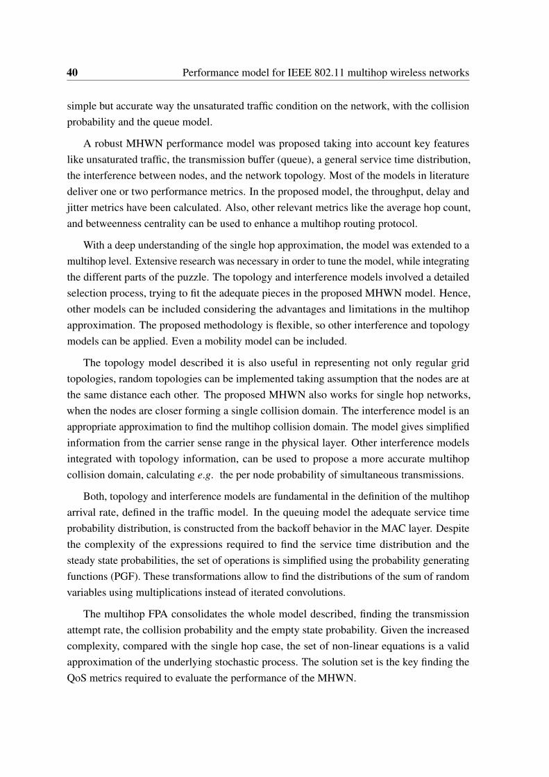
40 Performance model for IEEE 802.11 multihop wireless networks
simple but accurate way the unsaturated traffic condition on the network, with the collisionprobability and the queue model.
A robust MHWN performance model was proposed taking into account key featureslike unsaturated traffic, the transmission buffer (queue), a general service time distribution,the interference between nodes, and the network topology. Most of the models in literaturedeliver one or two performance metrics. In the proposed model, the throughput, delay andjitter metrics have been calculated. Also, other relevant metrics like the average hop count,and betweenness centrality can be used to enhance a multihop routing protocol.
With a deep understanding of the single hop approximation, the model was extended to amultihop level. Extensive research was necessary in order to tune the model, while integratingthe different parts of the puzzle. The topology and interference models involved a detailedselection process, trying to fit the adequate pieces in the proposed MHWN model. Hence,other models can be included considering the advantages and limitations in the multihopapproximation. The proposed methodology is flexible, so other interference and topologymodels can be applied. Even a mobility model can be included.
The topology model described it is also useful in representing not only regular gridtopologies, random topologies can be implemented taking assumption that the nodes are atthe same distance each other. The proposed MHWN also works for single hop networks,when the nodes are closer forming a single collision domain. The interference model is anappropriate approximation to find the multihop collision domain. The model gives simplifiedinformation from the carrier sense range in the physical layer. Other interference modelsintegrated with topology information, can be used to propose a more accurate multihopcollision domain, calculating e.g. the per node probability of simultaneous transmissions.
Both, topology and interference models are fundamental in the definition of the multihoparrival rate, defined in the traffic model. In the queuing model the adequate service timeprobability distribution, is constructed from the backoff behavior in the MAC layer. Despitethe complexity of the expressions required to find the service time distribution and thesteady state probabilities, the set of operations is simplified using the probability generatingfunctions (PGF). These transformations allow to find the distributions of the sum of randomvariables using multiplications instead of iterated convolutions.
The multihop FPA consolidates the whole model described, finding the transmissionattempt rate, the collision probability and the empty state probability. Given the increasedcomplexity, compared with the single hop case, the set of non-linear equations is a validapproximation of the underlying stochastic process. The solution set is the key finding theQoS metrics required to evaluate the performance of the MHWN.

2.8 Conclusions 41
The proposed MHWN model is useful in the design phase of a wireless campus network,to set the appropriate operational parameters, or after the wireless network is implemented, toevaluate different settings in the network. The model allows to evaluate different topologiesby simply defining the graph model, reducing time and costs in the network implementation.Other type of networks could be evaluated, like WSN or VANET, integrating in the MHWNmodel the appropriate assumptions, from the MAC layer of each implementation. EvenMAC protocol enhancements can be tested before implementation, to evaluate the impact inperformance of the network.

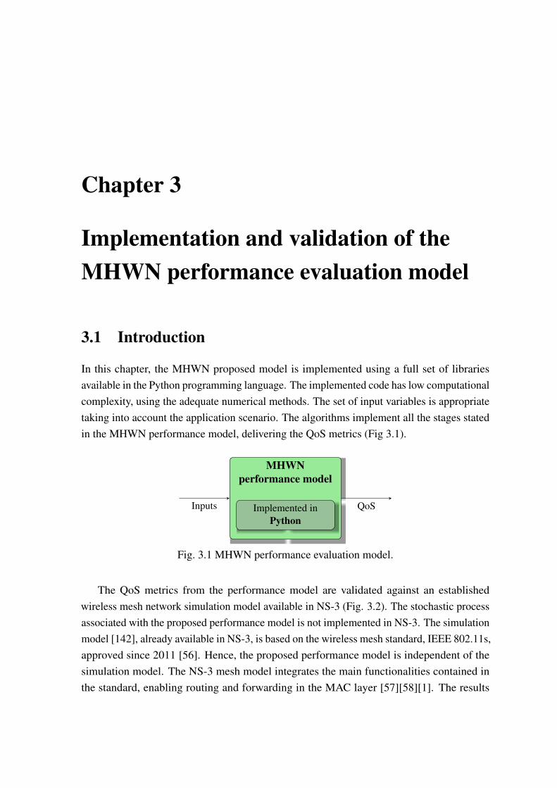
Chapter 3
Implementation and validation of theMHWN performance evaluation model
3.1 Introduction
In this chapter, the MHWN proposed model is implemented using a full set of librariesavailable in the Python programming language. The implemented code has low computationalcomplexity, using the adequate numerical methods. The set of input variables is appropriatetaking into account the application scenario. The algorithms implement all the stages statedin the MHWN performance model, delivering the QoS metrics (Fig 3.1).
MHWNperformance model
Implemented inPython
QoSInputs
Fig. 3.1 MHWN performance evaluation model.
The QoS metrics from the performance model are validated against an establishedwireless mesh network simulation model available in NS-3 (Fig. 3.2). The stochastic processassociated with the proposed performance model is not implemented in NS-3. The simulationmodel [142], already available in NS-3, is based on the wireless mesh standard, IEEE 802.11s,approved since 2011 [56]. Hence, the proposed performance model is independent of thesimulation model. The NS-3 mesh model integrates the main functionalities contained inthe standard, enabling routing and forwarding in the MAC layer [57][58][1]. The results
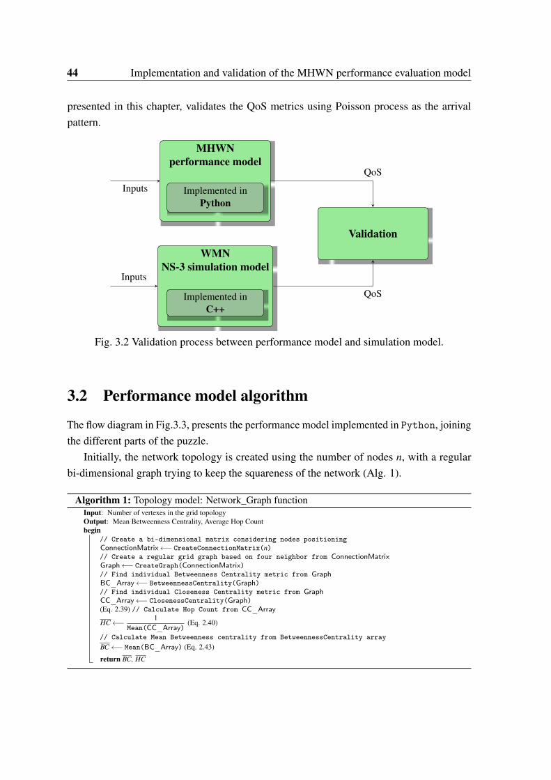
44 Implementation and validation of the MHWN performance evaluation model
presented in this chapter, validates the QoS metrics using Poisson process as the arrivalpattern.
MHWNperformance model
Implemented inPython
Inputs
WMNNS-3 simulation model
Implemented inC++
Inputs
Validation
QoS
QoS
Fig. 3.2 Validation process between performance model and simulation model.
3.2 Performance model algorithm
The flow diagram in Fig.3.3, presents the performance model implemented in Python, joiningthe different parts of the puzzle.
Initially, the network topology is created using the number of nodes n, with a regularbi-dimensional graph trying to keep the squareness of the network (Alg. 1).
Algorithm 1: Topology model: Network_Graph functionInput: Number of vertexes in the grid topologyOutput: Mean Betweenness Centrality, Average Hop Countbegin
// Create a bi-dimensional matrix considering nodes positioningConnectionMatrix←− CreateConnectionMatrix(n)// Create a regular grid graph based on four neighbor from ConnectionMatrixGraph←− CreateGraph(ConnectionMatrix)// Find individual Betweenness Centrality metric from GraphBC_Array←− BetweennessCentrality(Graph)// Find individual Closeness Centrality metric from GraphCC_Array←− ClosenessCentrality(Graph)(Eq. 2.39) // Calculate Hop Count from CC_Array
HC←− 1Mean(CC_Array)
(Eq. 2.40)
// Calculate Mean Betweenness centrality from BetweennessCentrality arrayBC←− Mean(BC_Array) (Eq. 2.43)
return BC, HC
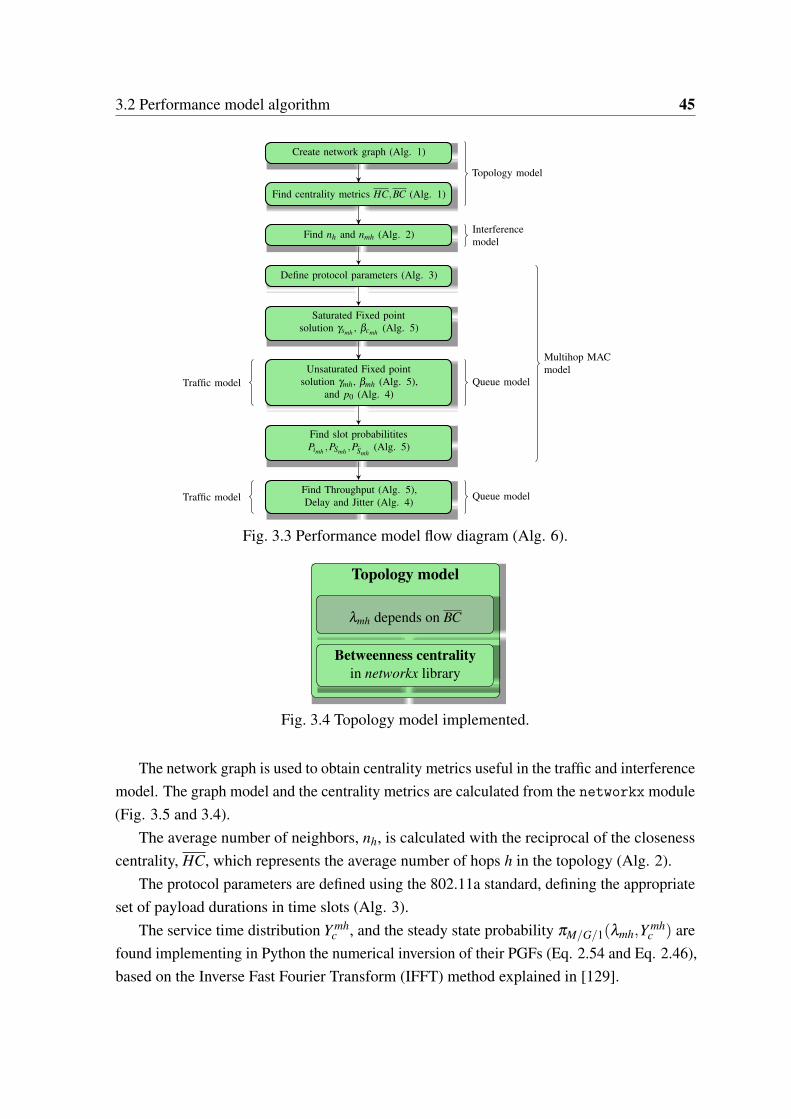
3.2 Performance model algorithm 45
Create network graph (Alg. 1)
Find centrality metrics HC,BC (Alg. 1)
Find nh and nmh (Alg. 2)
Define protocol parameters (Alg. 3)
Saturated Fixed pointsolution γsmh , βcmh (Alg. 5)
Unsaturated Fixed pointsolution γmh, βmh (Alg. 5),
and p0 (Alg. 4)
Find slot probabilititesPimh ,PSmh ,PSmh
(Alg. 5)
Find Throughput (Alg. 5),Delay and Jitter (Alg. 4)
Multihop MACmodel
Queue model
Topology model
Interferencemodel
Traffic model
Traffic model Queue model
Fig. 3.3 Performance model flow diagram (Alg. 6).
Topology model
λmh depends on BC
Betweenness centralityin networkx library
Fig. 3.4 Topology model implemented.
The network graph is used to obtain centrality metrics useful in the traffic and interferencemodel. The graph model and the centrality metrics are calculated from the networkx module(Fig. 3.5 and 3.4).
The average number of neighbors, nh, is calculated with the reciprocal of the closenesscentrality, HC, which represents the average number of hops h in the topology (Alg. 2).
The protocol parameters are defined using the 802.11a standard, defining the appropriateset of payload durations in time slots (Alg. 3).
The service time distribution Y mhc , and the steady state probability πM/G/1(λmh,Y mh
c ) arefound implementing in Python the numerical inversion of their PGFs (Eq. 2.54 and Eq. 2.46),based on the Inverse Fast Fourier Transform (IFFT) method explained in [129].
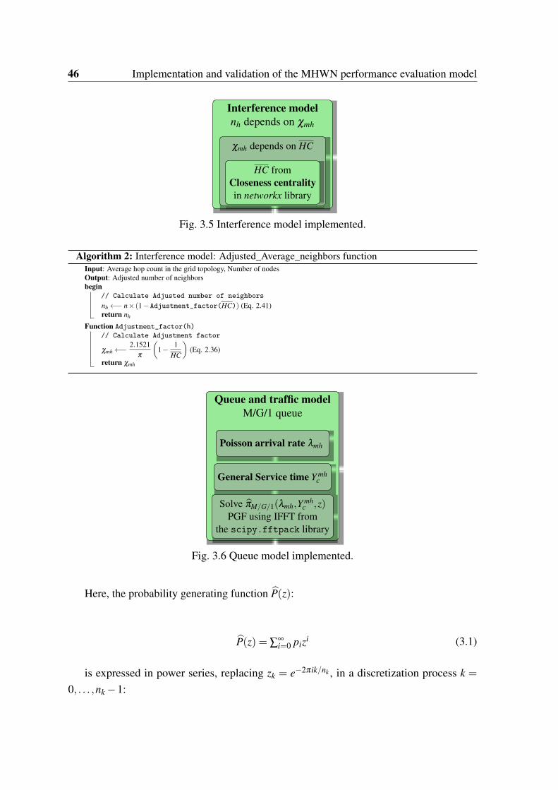
46 Implementation and validation of the MHWN performance evaluation model
Interference modelnh depends on χmh
χmh depends on HC
HC fromCloseness centralityin networkx library
Fig. 3.5 Interference model implemented.
Algorithm 2: Interference model: Adjusted_Average_neighbors functionInput: Average hop count in the grid topology, Number of nodesOutput: Adjusted number of neighborsbegin
// Calculate Adjusted number of neighborsnh←− n× (1−Adjustment_factor(HC)) (Eq. 2.41)return nh
Function Adjustment_factor(h)// Calculate Adjustment factor
χmh←−2.1521
π
(1− 1
HC
)(Eq. 2.36)
return χmh
Queue and traffic modelM/G/1 queue
Poisson arrival rate λmh
General Service time Y mhc
Solve πM/G/1(λmh,Y mhc ,z)
PGF using IFFT fromthe scipy.fftpack library
Fig. 3.6 Queue model implemented.
Here, the probability generating function P(z):
P(z) = ∑∞i=0 pizi (3.1)
is expressed in power series, replacing zk = e−2πik/nk , in a discretization process k =
0, . . . ,nk−1:
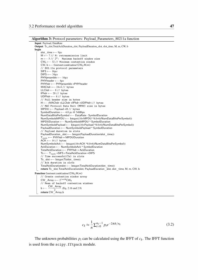
3.2 Performance model algorithm 47
Algorithm 3: Protocol parameters: Payload_Parameters_80211a functionInput: Payload, DataRateOutput: Ts_slot,TotalAckDuration_slot, PayloadDuration_slot, slot_time, M, m, CW, bbegin
slot_time←− 9µsM←− 7 // M: retransmission limitm←− 5 // 2m: Maximum backoff window sizeCW0 ←− 32 // Minimum contention windowCW, b←− ContentionWindow(CW0,M,m)// 802.11a protocol parametersSIFS←− 16µsDIFS←− 34µsPHYpreamble←− 16µsPHYheader←− 4µsPHYhdr←− PHYpreamble +PHYheaderMAChdr←− 24+4 // bytesLLChdr←− 8 // bytesIPhdr←− 20 // bytesUDPhdr←− 8 // bytes// Full header size in bytesH←− (MAChdr +LLChdr +IPhdr +UDPhdr) // bytes// MAC Protocol Data Unit (MPDU) size in bytesMPDU←− Payload +H // bytesSymbolDuration←− 4.0 µs @ 54MbpsNumDataBitsPerSymbol←− DataRate · SymbolDurationNumSymbolsMPDU←− Integer((16+MPDU *8.0+6)/NumDataBitsPerSymbol))MPDUDuration←− NumSymbolsMPDU * SymbolDurationNumSymbolsPayload←− Integer((16+Payload *8.0+6)/NumDataBitsPerSymbol))PayloadDuration←− NumSymbolsPayload * SymbolDuration// Payload duration in slotsPayloadDuration_slot←− Integer(PayloadDuration/slot_time))Tmpdu ←− PHYhdr + MPDUDurationACK←− 14 // bytesNumSymbolsAck←− Integer((16+ACK *8.0+6)/NumDataBitsPerSymbol))AckDuration←− NumSymbolsAck * SymbolDurationTotalAckDuration←− PHYhdr + AckDurationTs←− Tmpdu +SIFS +TotalAckDuration +DIFS// Time successful(Ts) in slotsTs_slot←− Integer(Ts/slot_time))// Ack duration in slotsTotalAckDurationslot←− Integer(TotalAckDuration/slot_time))return Ts_slot,TotalAckDurationslot, PayloadDuration_slot, slot_time, M, m, CW, b
Function ContentionWindow(CW0,M,m)// Create contention window arrayCW_Array←− 21:m:MCW0// Mean of backoff contention windows
b←− CW_Array2
(Eq. 2.16 and 2.9)
return CW_Array,b
ck ≈1n
∑nk−1i=0 pie−2πik/nk (3.2)
The unknown probabilities pi can be calculated using the IFFT of ck. The IFFT functionis used from the scipy.fftpack module.
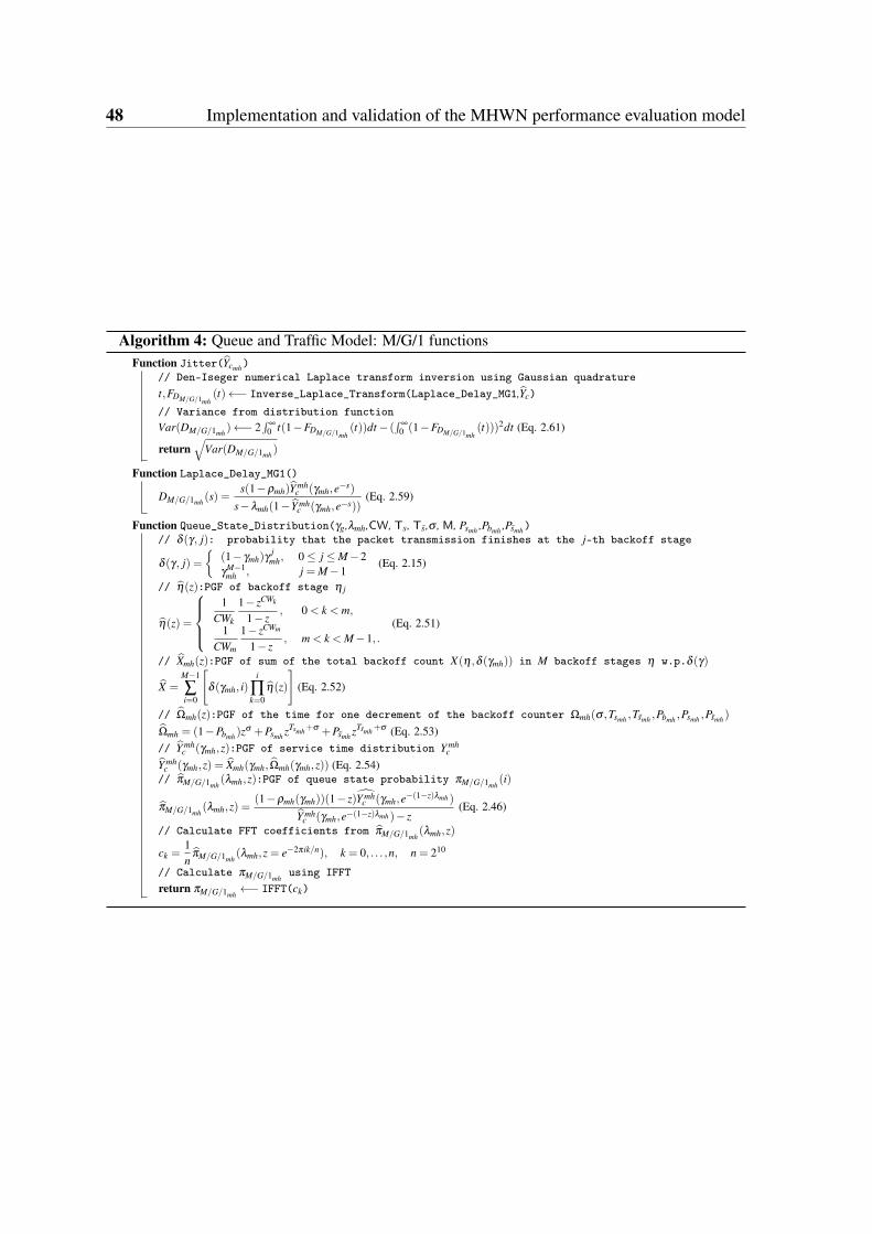
48 Implementation and validation of the MHWN performance evaluation model
Algorithm 4: Queue and Traffic Model: M/G/1 functionsFunction Jitter(Ycmh)
// Den-Iseger numerical Laplace transform inversion using Gaussian quadraturet,FDM/G/1mh
(t)←− Inverse_Laplace_Transform(Laplace_Delay_MG1,Yc)
// Variance from distribution functionVar(DM/G/1mh
)←− 2∫
∞
0 t(1−FDM/G/1mh(t))dt− (
∫∞
0 (1−FDM/G/1mh(t)))2dt (Eq. 2.61)
return√
Var(DM/G/1mh)
Function Laplace_Delay_MG1()
DM/G/1mh(s) =
s(1−ρmh)Y mhc (γmh,e−s)
s−λmh(1− Y mhc (γmh,e−s))
(Eq. 2.59)
Function Queue_State_Distribution(γg,λmh,CW, Ts, Ts,σ , M, Psmh ,Pbmh ,Psmh)// δ (γ, j): probability that the packet transmission finishes at the j-th backoff stage
δ (γ, j) =
(1− γmh)γj
mh, 0≤ j ≤M−2γ
M−1mh , j = M−1
(Eq. 2.15)
// η(z):PGF of backoff stage η j
η(z) =
1
CWk
1− zCWk
1− z, 0 < k < m,
1CWm
1− zCWm
1− z, m < k < M−1, .
(Eq. 2.51)
// Xmh(z):PGF of sum of the total backoff count X(η ,δ (γmh)) in M backoff stages η w.p.δ (γ)
X =M−1
∑i=0
[δ (γmh, i)
i
∏k=0
η(z)
](Eq. 2.52)
// Ωmh(z):PGF of the time for one decrement of the backoff counter Ωmh(σ ,Tsmh ,Tsmh ,Pbmh ,Psmh ,Psmh )
Ωmh = (1−Pbmh )zσ +Psmh zTsmh+σ +Psmh zTsmh+σ (Eq. 2.53)
// Y mhc (γmh,z):PGF of service time distribution Y mh
c
Y mhc (γmh,z) = Xmh(γmh,Ωmh(γmh,z)) (Eq. 2.54)// πM/G/1mh
(λmh,z):PGF of queue state probability πM/G/1mh(i)
πM/G/1mh(λmh,z) =
(1−ρmh(γmh))(1− z)Y mhc (γmh,e−(1−z)λmh )
Y mhc (γmh,e−(1−z)λmh )− z
(Eq. 2.46)
// Calculate FFT coefficients from πM/G/1mh(λmh,z)
ck =1n
πM/G/1mh(λmh,z = e−2πik/n), k = 0, . . . ,n, n = 210
// Calculate πM/G/1mhusing IFFT
return πM/G/1mh←− IFFT(ck)
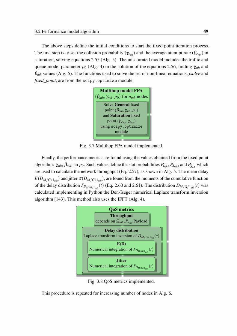
3.2 Performance model algorithm 49
The above steps define the initial conditions to start the fixed point iteration process.The first step is to set the collision probability (γsmh) and the average attempt rate (βcmh) insaturation, solving equations 2.55 (Alg. 5). The unsaturated model includes the traffic andqueue model parameter p0 (Alg. 4) in the solution of the equations 2.56, finding γmh andβmh values (Alg. 5). The functions used to solve the set of non-linear equations, fsolve andfixed_point, are from the scipy.optimize module.
Multihop model FPA(βmh,γmh, p0) for nmh nodes
Solve General fixedpoint (βmh,γmh, p0)
and Saturation fixedpoint (βcmh ,γsmh)
using scipy.optimizemodule
Fig. 3.7 Multihop FPA model implemented.
Finally, the performance metrics are found using the values obtained from the fixed pointalgorithm: γmh, βmh, an p0. Such values define the slot probabilities Pimh , PSmh , and PSmh
whichare used to calculate the network throughput (Eq. 2.57), as shown in Alg. 5. The mean delayE(DM/G/1mh
) and jitter σ(DM/G/1mh), are found from the moments of the cumulative function
of the delay distribution FDM/G/1mh(t) (Eq. 2.60 and 2.61). The distribution DM/G/1mh
(t) wascalculated implementing in Python the Den-Iseger numerical Laplace transform inversionalgorithm [143]. This method also uses the IFFT (Alg. 4).
QoS metricsThroughput
depends on Ωmh,PSmh ,Payload
Delay distributionLaplace transform inversion of DM/G/1mh(s)
JitterNumerical integration of FDM/G/1mh
(t)
E(D)Numerical integration of FDM/G/1mh
(t)
Fig. 3.8 QoS metrics implemented.
This procedure is repeated for increasing number of nodes in Alg. 6.
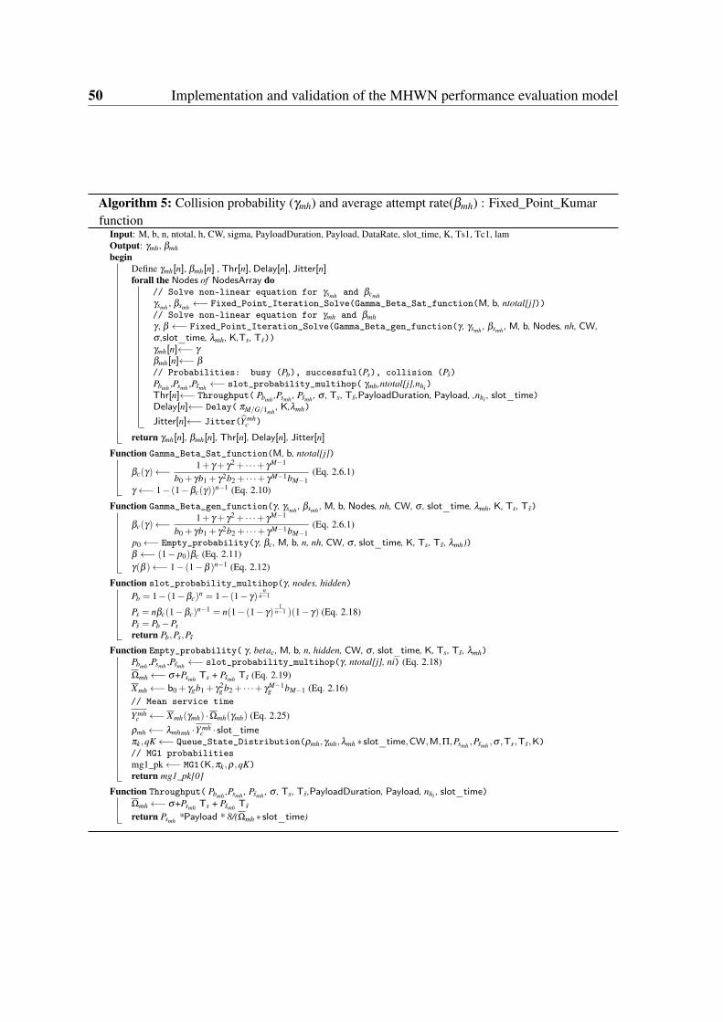
50 Implementation and validation of the MHWN performance evaluation model
Algorithm 5: Collision probability (γmh) and average attempt rate(βmh) : Fixed_Point_Kumarfunction
Input: M, b, n, ntotal, h, CW, sigma, PayloadDuration, Payload, DataRate, slot_time, K, Ts1, Tc1, lamOutput: γmh, βmhbegin
Define γmh[n], βmh[n] , Thr[n], Delay[n], Jitter[n]forall the Nodes of NodesArray do
// Solve non-linear equation for γsmh and βcmhγsmh , βsmh ←− Fixed_Point_Iteration_Solve(Gamma_Beta_Sat_function(M, b, ntotal[j]))// Solve non-linear equation for γmh and βmhγ , β ←− Fixed_Point_Iteration_Solve(Gamma_Beta_gen_function(γ , γsmh , βsmh , M, b, Nodes, nh, CW,σ ,slot_time, λmh, K,Ts, Ts))γmh[n]←− γ
βmh[n]←− β
// Probabilities: busy (Pb), successful(Ps), collision (Ps)Pbmh ,Psmh ,Psmh ←− slot_probability_multihop( γmh,ntotal[j],nhi)Thr[n]←− Throughput( Pbmh ,Psmh , Psmh , σ , Ts, Ts,PayloadDuration, Payload, ,nhi , slot_time)Delay[n]←− Delay( πM/G/1mh
, K,λmh)Jitter[n]←− Jitter(Y mh
c )
return γmh[n], βmh[n], Thr[n], Delay[n], Jitter[n]
Function Gamma_Beta_Sat_function(M, b, ntotal[j])
βc(γ)←−1+ γ + γ2 + · · ·+ γM−1
b0 + γb1 + γ2b2 + · · ·+ γM−1bM−1(Eq. 2.6.1)
γ ←− 1− (1−βc(γ))n−1 (Eq. 2.10)
Function Gamma_Beta_gen_function(γ , γsmh , βsmh , M, b, Nodes, nh, CW, σ , slot_time, λmh, K, Ts, Ts)
βc(γ)←−1+ γ + γ2 + · · ·+ γM−1
b0 + γb1 + γ2b2 + · · ·+ γM−1bM−1(Eq. 2.6.1)
p0←− Empty_probability(γ , βc, M, b, n, nh, CW, σ , slot_time, K, Ts, Ts, λmh))β ←− (1− p0)βc (Eq. 2.11)γ(β )←− 1− (1−β )n−1 (Eq. 2.12)
Function slot_probability_multihop(γ , nodes, hidden)Pb = 1− (1−βc)
n = 1− (1− γ)n
n−1
Ps = nβc(1−βc)n−1 = n(1− (1− γ)
1n−1 )(1− γ) (Eq. 2.18)
Ps = Pb−Psreturn Pb,Ps,Ps
Function Empty_probability( γ , betac, M, b, n, hidden, CW, σ , slot_time, K, Ts, Ts, λmh)Pbmh ,Psmh ,Psmh ←− slot_probability_multihop(γ , ntotal[j], ni) (Eq. 2.18)Ωmh←− σ+Psmh Ts + Psmh Ts (Eq. 2.19)Xmh←− b0 + γgb1 + γ2
g b2 + · · ·+ γM−1g bM−1 (Eq. 2.16)
// Mean service timeY mh
c ←− Xmh(γmh) ·Ωmh(γmh) (Eq. 2.25)ρmh←− λmhmh ·Y mh
c · slot_timeπk,qK←− Queue_State_Distribution(ρmh,γmh,λmh ∗ slot_time,CW,M,Π,Psmh ,Psmh ,σ ,Ts,Ts,K)// MG1 probabilitiesmg1_pk←− MG1(K,πk,ρ,qK)return mg1_pk[0]
Function Throughput( Pbmh ,Psmh , Psmh , σ , Ts, Ts,PayloadDuration, Payload, nhi , slot_time)Ωmh←− σ+Psmh Ts + Psmh Ts
return Psmh *Payload * 8/(Ωmh ∗ slot_time)
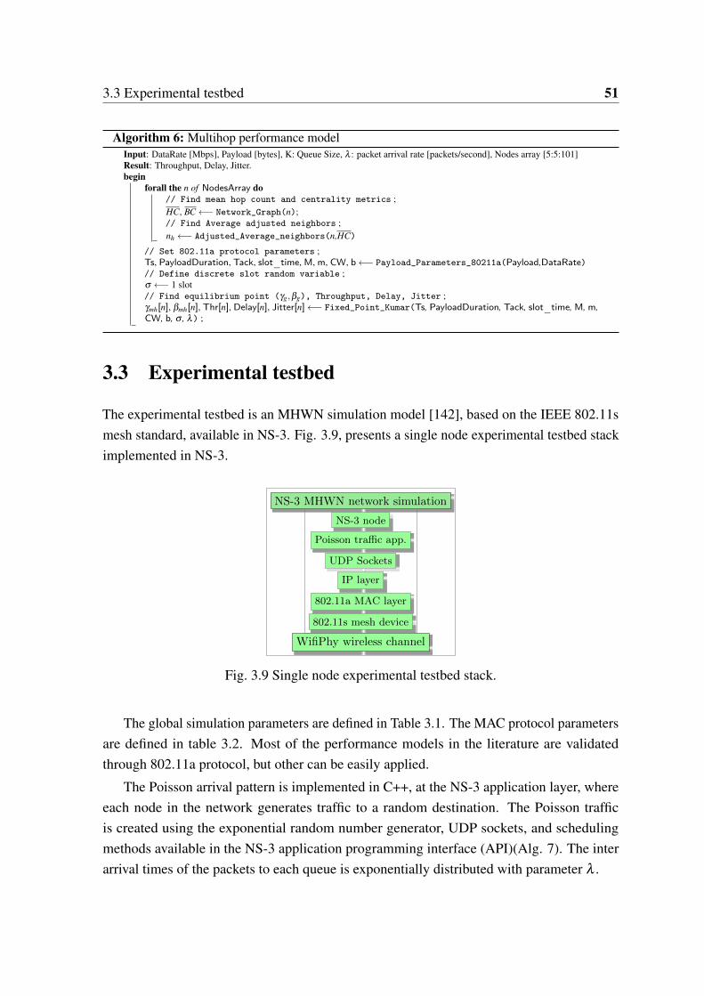
3.3 Experimental testbed 51
Algorithm 6: Multihop performance modelInput: DataRate [Mbps], Payload [bytes], K: Queue Size, λ : packet arrival rate [packets/second], Nodes array [5:5:101]Result: Throughput, Delay, Jitter.begin
forall the n of NodesArray do// Find mean hop count and centrality metrics ;HC, BC←− Network_Graph(n);// Find Average adjusted neighbors ;nh ←− Adjusted_Average_neighbors(n,HC)
// Set 802.11a protocol parameters ;Ts, PayloadDuration, Tack, slot_time, M, m, CW, b←− Payload_Parameters_80211a(Payload,DataRate)// Define discrete slot random variable ;σ ←− 1 slot// Find equilibrium point (γg,βg), Throughput, Delay, Jitter ;γmh[n], βmh[n], Thr[n], Delay[n], Jitter[n]←− Fixed_Point_Kumar(Ts, PayloadDuration, Tack, slot_time, M, m,CW, b, σ , λ) ;
3.3 Experimental testbed
The experimental testbed is an MHWN simulation model [142], based on the IEEE 802.11smesh standard, available in NS-3. Fig. 3.9, presents a single node experimental testbed stackimplemented in NS-3.
NS-3 MHWN network simulation
NS-3 node
Poisson traffic app.
UDP Sockets
IP layer
802.11a MAC layer
802.11s mesh device
WifiPhy wireless channel
Fig. 3.9 Single node experimental testbed stack.
The global simulation parameters are defined in Table 3.1. The MAC protocol parametersare defined in table 3.2. Most of the performance models in the literature are validatedthrough 802.11a protocol, but other can be easily applied.
The Poisson arrival pattern is implemented in C++, at the NS-3 application layer, whereeach node in the network generates traffic to a random destination. The Poisson trafficis created using the exponential random number generator, UDP sockets, and schedulingmethods available in the NS-3 application programming interface (API)(Alg. 7). The interarrival times of the packets to each queue is exponentially distributed with parameter λ .
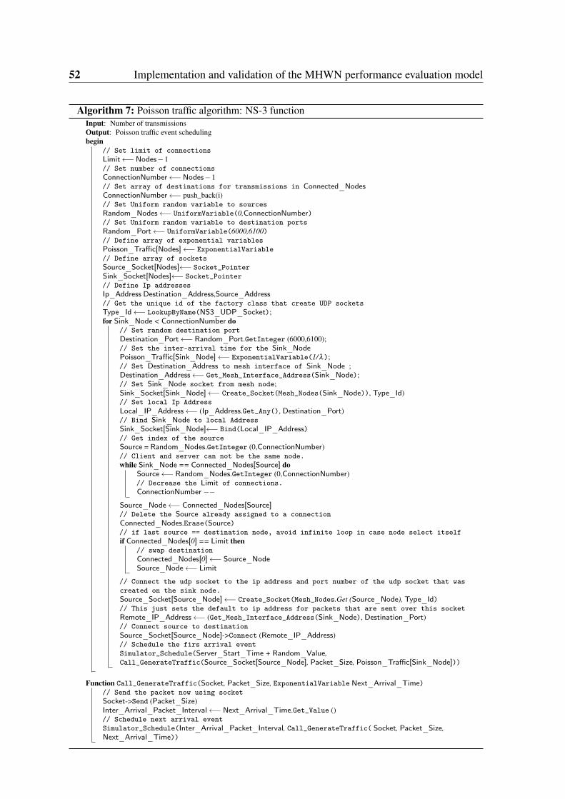
52 Implementation and validation of the MHWN performance evaluation model
Algorithm 7: Poisson traffic algorithm: NS-3 functionInput: Number of transmissionsOutput: Poisson traffic event schedulingbegin
// Set limit of connectionsLimit←−Nodes−1// Set number of connectionsConnectionNumber←−Nodes−1// Set array of destinations for transmissions in Connected_NodesConnectionNumber←− push_back(i)// Set Uniform random variable to sourcesRandom_Nodes←− UniformVariable(0,ConnectionNumber)// Set Uniform random variable to destination portsRandom_Port←− UniformVariable(6000,6100)// Define array of exponential variablesPoisson_Traffic[Nodes]←− ExponentialVariable// Define array of socketsSource_Socket[Nodes]←− Socket_PointerSink_Socket[Nodes]←− Socket_Pointer// Define Ip addressesIp_Address Destination_Address,Source_Address// Get the unique id of the factory class that create UDP socketsType_Id←− LookupByName(NS3_UDP_Socket);for Sink_Node < ConnectionNumber do
// Set random destination portDestination_Port←− Random_Port.GetInteger (6000,6100);// Set the inter-arrival time for the Sink_NodePoisson_Traffic[Sink_Node]←− ExponentialVariable(1/λ);// Set Destination_Address to mesh interface of Sink_Node ;Destination_Address←− Get_Mesh_Interface_Address(Sink_Node);// Set Sink_Node socket from mesh node;Sink_Socket[Sink_Node]←− Create_Socket(Mesh_Nodes(Sink_Node)), Type_Id)// Set local Ip AddressLocal_IP_Address←− (Ip_Address.Get_Any(), Destination_Port)// Bind Sink_Node to local AddressSink_Socket[Sink_Node]←− Bind(Local_IP_Address)// Get index of the sourceSource = Random_Nodes.GetInteger (0,ConnectionNumber)// Client and server can not be the same node.while Sink_Node == Connected_Nodes[Source] do
Source←− Random_Nodes.GetInteger (0,ConnectionNumber)// Decrease the Limit of connections.ConnectionNumber −−
Source_Node←− Connected_Nodes[Source]// Delete the Source already assigned to a connectionConnected_Nodes.Erase(Source)// if last source == destination node, avoid infinite loop in case node select itselfif Connected_Nodes[0] == Limit then
// swap destinationConnected_Nodes[0]←− Source_NodeSource_Node←− Limit
// Connect the udp socket to the ip address and port number of the udp socket that wascreated on the sink node.Source_Socket[Source_Node]←− Create_Socket(Mesh_Nodes.Get (Source_Node), Type_Id)// This just sets the default to ip address for packets that are sent over this socketRemote_IP_Address←− (Get_Mesh_Interface_Address(Sink_Node), Destination_Port)// Connect source to destinationSource_Socket[Source_Node]->Connect (Remote_IP_Address)// Schedule the firs arrival eventSimulator_Schedule(Server_Start_Time + Random_Value,Call_GenerateTraffic(Source_Socket[Source_Node], Packet_Size, Poisson_Traffic[Sink_Node]))
Function Call_GenerateTraffic(Socket, Packet_Size, ExponentialVariable Next_Arrival_Time)// Send the packet now using socketSocket->Send (Packet_Size)Inter_Arrival_Packet_Interval←− Next_Arrival_Time.Get_Value ()// Schedule next arrival eventSimulator_Schedule(Inter_Arrival_Packet_Interval, Call_GenerateTraffic( Socket, Packet_Size,Next_Arrival_Time))
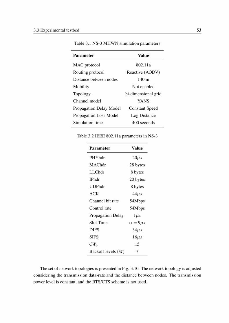
3.3 Experimental testbed 53
Table 3.1 NS-3 MHWN simulation parameters
Parameter Value
MAC protocol 802.11a
Routing protocol Reactive (AODV)
Distance between nodes 140 m
Mobility Not enabled
Topology bi-dimensional grid
Channel model YANS
Propagation Delay Model Constant Speed
Propagation Loss Model Log Distance
Simulation time 400 seconds
Table 3.2 IEEE 802.11a parameters in NS-3
Parameter Value
PHYhdr 20µs
MAChdr 28 bytes
LLChdr 8 bytes
IPhdr 20 bytes
UDPhdr 8 bytes
ACK 44µs
Channel bit rate 54Mbps
Control rate 54Mbps
Propagation Delay 1µs
Slot Time σ = 9µs
DIFS 34µs
SIFS 16µs
CW0 15
Backoff levels (M) 7
The set of network topologies is presented in Fig. 3.10. The network topology is adjustedconsidering the transmission data-rate and the distance between nodes. The transmissionpower level is constant, and the RTS/CTS scheme is not used.
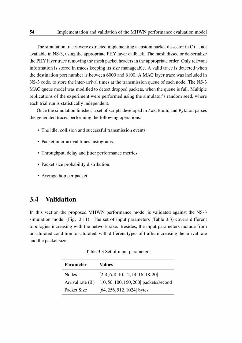
54 Implementation and validation of the MHWN performance evaluation model
The simulation traces were extracted implementing a custom packet dissector in C++, notavailable in NS-3, using the appropriate PHY layer callback. The mesh dissector de-serializethe PHY layer trace removing the mesh packet headers in the appropriate order. Only relevantinformation is stored in traces keeping its size manageable. A valid trace is detected whenthe destination port number is between 6000 and 6100. A MAC layer trace was included inNS-3 code, to store the inter-arrival times at the transmission queue of each node. The NS-3MAC queue model was modified to detect dropped packets, when the queue is full. Multiplereplications of the experiment were performed using the simulator’s random seed, whereeach trial run is statistically independent.
Once the simulation finishes, a set of scripts developed in Awk, Bash, and Python parsesthe generated traces performing the following operations:
• The idle, collision and successful transmission events.
• Packet inter-arrival times histograms.
• Throughput, delay and jitter performance metrics.
• Packet size probability distribution.
• Average hop per packet.
3.4 Validation
In this section the proposed MHWN performance model is validated against the NS-3simulation model (Fig. 3.11). The set of input parameters (Table 3.3) covers differenttopologies increasing with the network size. Besides, the input parameters include fromunsaturated condition to saturated, with different types of traffic increasing the arrival rateand the packet size.
Table 3.3 Set of input parameters
Parameter Values
Nodes [2,4,6,8,10,12,14,16,18,20]
Arrival rate (λ ) [10,50,100,150,200] packets/second
Packet Size [64,256,512,1024] bytes
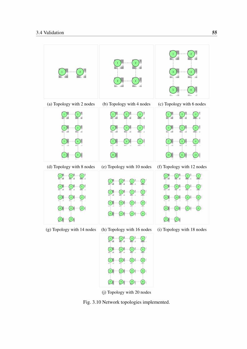
3.4 Validation 55
1 2
(a) Topology with 2 nodes
1 2
3 4
(b) Topology with 4 nodes
1 2
3 4
5 6
(c) Topology with 6 nodes
1 2
3 4
5 6
7 8
(d) Topology with 8 nodes
1 2 3
4 5 6
7 8 9
10
(e) Topology with 10 nodes
1 2 3
4 5 6
7 8 9
10 11 12
(f) Topology with 12 nodes
1 2 3
4 5 6
7 8 9
10 11 12
13 14
(g) Topology with 14 nodes
1 2 3 4
5 6 7 8
9 10 11 12
13 14 15 16
(h) Topology with 16 nodes
1 2 3 4
5 6 7 8
9 10 11 12
13 14 15 16
17 18
(i) Topology with 18 nodes
1 2 3 4
5 6 7 8
9 10 11 12
13 14 15 16
17 18 19 20
(j) Topology with 20 nodes
Fig. 3.10 Network topologies implemented.
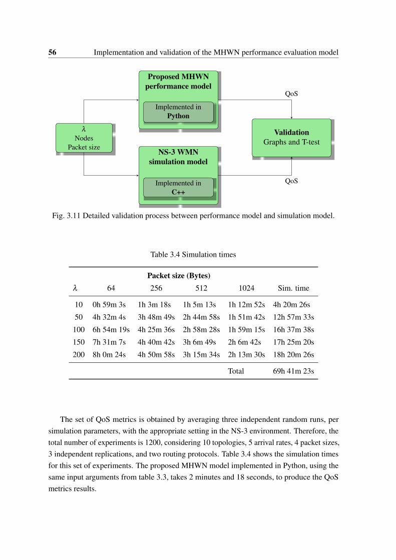
56 Implementation and validation of the MHWN performance evaluation model
Proposed MHWNperformance model
Implemented inPython
λ
NodesPacket size NS-3 WMN
simulation model
Implemented inC++
ValidationGraphs and T-test
QoS
QoS
Fig. 3.11 Detailed validation process between performance model and simulation model.
Table 3.4 Simulation times
Packet size (Bytes)λ 64 256 512 1024 Sim. time
10 0h 59m 3s 1h 3m 18s 1h 5m 13s 1h 12m 52s 4h 20m 26s
50 4h 32m 4s 3h 48m 49s 2h 44m 58s 1h 51m 42s 12h 57m 33s
100 6h 54m 19s 4h 25m 36s 2h 58m 28s 1h 59m 15s 16h 37m 38s
150 7h 31m 7s 4h 40m 42s 3h 6m 49s 2h 6m 42s 17h 25m 20s
200 8h 0m 24s 4h 50m 58s 3h 15m 34s 2h 13m 30s 18h 20m 26s
Total 69h 41m 23s
The set of QoS metrics is obtained by averaging three independent random runs, persimulation parameters, with the appropriate setting in the NS-3 environment. Therefore, thetotal number of experiments is 1200, considering 10 topologies, 5 arrival rates, 4 packet sizes,3 independent replications, and two routing protocols. Table 3.4 shows the simulation timesfor this set of experiments. The proposed MHWN model implemented in Python, using thesame input arguments from table 3.3, takes 2 minutes and 18 seconds, to produce the QoSmetrics results.
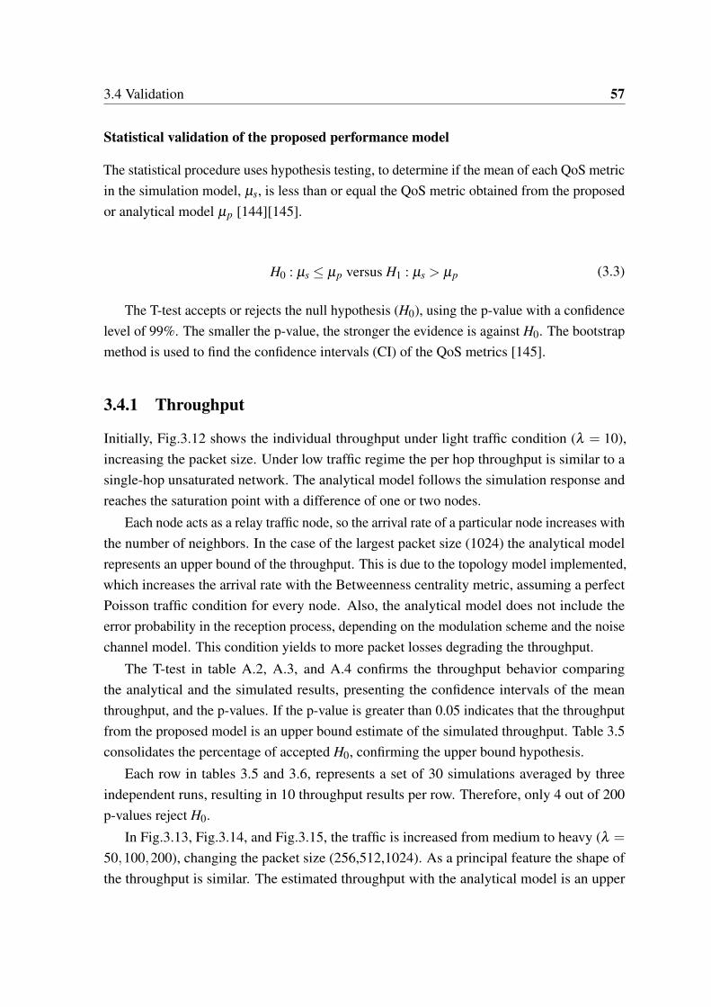
3.4 Validation 57
Statistical validation of the proposed performance model
The statistical procedure uses hypothesis testing, to determine if the mean of each QoS metricin the simulation model, µs, is less than or equal the QoS metric obtained from the proposedor analytical model µp [144][145].
H0 : µs ≤ µp versus H1 : µs > µp (3.3)
The T-test accepts or rejects the null hypothesis (H0), using the p-value with a confidencelevel of 99%. The smaller the p-value, the stronger the evidence is against H0. The bootstrapmethod is used to find the confidence intervals (CI) of the QoS metrics [145].
3.4.1 Throughput
Initially, Fig.3.12 shows the individual throughput under light traffic condition (λ = 10),increasing the packet size. Under low traffic regime the per hop throughput is similar to asingle-hop unsaturated network. The analytical model follows the simulation response andreaches the saturation point with a difference of one or two nodes.
Each node acts as a relay traffic node, so the arrival rate of a particular node increases withthe number of neighbors. In the case of the largest packet size (1024) the analytical modelrepresents an upper bound of the throughput. This is due to the topology model implemented,which increases the arrival rate with the Betweenness centrality metric, assuming a perfectPoisson traffic condition for every node. Also, the analytical model does not include theerror probability in the reception process, depending on the modulation scheme and the noisechannel model. This condition yields to more packet losses degrading the throughput.
The T-test in table A.2, A.3, and A.4 confirms the throughput behavior comparingthe analytical and the simulated results, presenting the confidence intervals of the meanthroughput, and the p-values. If the p-value is greater than 0.05 indicates that the throughputfrom the proposed model is an upper bound estimate of the simulated throughput. Table 3.5consolidates the percentage of accepted H0, confirming the upper bound hypothesis.
Each row in tables 3.5 and 3.6, represents a set of 30 simulations averaged by threeindependent runs, resulting in 10 throughput results per row. Therefore, only 4 out of 200p-values reject H0.
In Fig.3.13, Fig.3.14, and Fig.3.15, the traffic is increased from medium to heavy (λ =
50,100,200), changing the packet size (256,512,1024). As a principal feature the shape ofthe throughput is similar. The estimated throughput with the analytical model is an upper
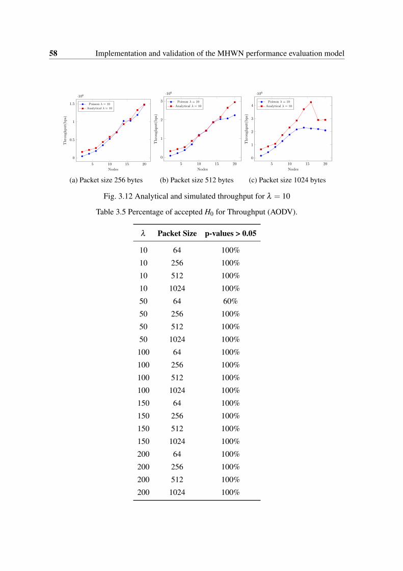
58 Implementation and validation of the MHWN performance evaluation model
5 10 15 20
0
0.5
1
1.5
·106
Nodes
Through
put(bps)
Poisson λ = 10
Analytical λ = 10
(a) Packet size 256 bytes
5 10 15 20
0
1
2
3
·106
Nodes
Through
put(bps)
Poisson λ = 10
Analytical λ = 10
(b) Packet size 512 bytes
5 10 15 20
0
1
2
3
4
·106
Nodes
Through
put(bps)
Poisson λ = 10
Analytical λ = 10
(c) Packet size 1024 bytes
Fig. 3.12 Analytical and simulated throughput for λ = 10
Table 3.5 Percentage of accepted H0 for Throughput (AODV).
λ Packet Size p-values > 0.05
10 64 100%
10 256 100%
10 512 100%
10 1024 100%
50 64 60%
50 256 100%
50 512 100%
50 1024 100%
100 64 100%
100 256 100%
100 512 100%
100 1024 100%
150 64 100%
150 256 100%
150 512 100%
150 1024 100%
200 64 100%
200 256 100%
200 512 100%
200 1024 100%
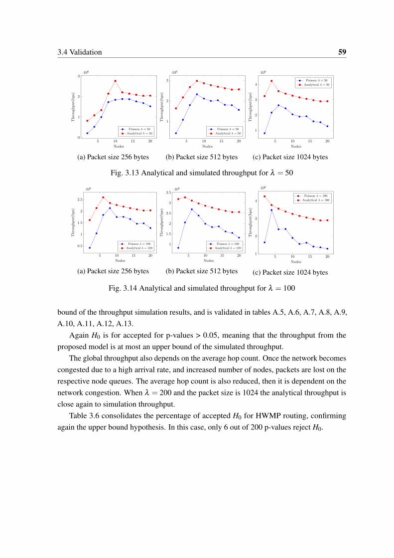
3.4 Validation 59
5 10 15 200
1
2
3·106
Nodes
Through
put(bps)
Poisson λ = 50
Analytical λ = 50
(a) Packet size 256 bytes
5 10 15 20
1
2
3
·106
Nodes
Through
put(bps)
Poisson λ = 50
Analytical λ = 50
(b) Packet size 512 bytes
5 10 15 20
1
2
3
4
·106
Nodes
Through
put(bps)
Poisson λ = 50
Analytical λ = 50
(c) Packet size 1024 bytes
Fig. 3.13 Analytical and simulated throughput for λ = 50
5 10 15 20
0.5
1
1.5
2
2.5
·106
Nodes
Through
put(bps)
Poisson λ = 100
Analytical λ = 100
(a) Packet size 256 bytes
5 10 15 20
1
1.5
2
2.5
3
3.5·106
Nodes
Through
put(bps)
Poisson λ = 100
Analytical λ = 100
(b) Packet size 512 bytes
5 10 15 201
2
3
4
·106
Nodes
Through
put(bps)
Poisson λ = 100
Analytical λ = 100
(c) Packet size 1024 bytes
Fig. 3.14 Analytical and simulated throughput for λ = 100
bound of the throughput simulation results, and is validated in tables A.5, A.6, A.7, A.8, A.9,A.10, A.11, A.12, A.13.
Again H0 is for accepted for p-values > 0.05, meaning that the throughput from theproposed model is at most an upper bound of the simulated throughput.
The global throughput also depends on the average hop count. Once the network becomescongested due to a high arrival rate, and increased number of nodes, packets are lost on therespective node queues. The average hop count is also reduced, then it is dependent on thenetwork congestion. When λ = 200 and the packet size is 1024 the analytical throughput isclose again to simulation throughput.
Table 3.6 consolidates the percentage of accepted H0 for HWMP routing, confirmingagain the upper bound hypothesis. In this case, only 6 out of 200 p-values reject H0.
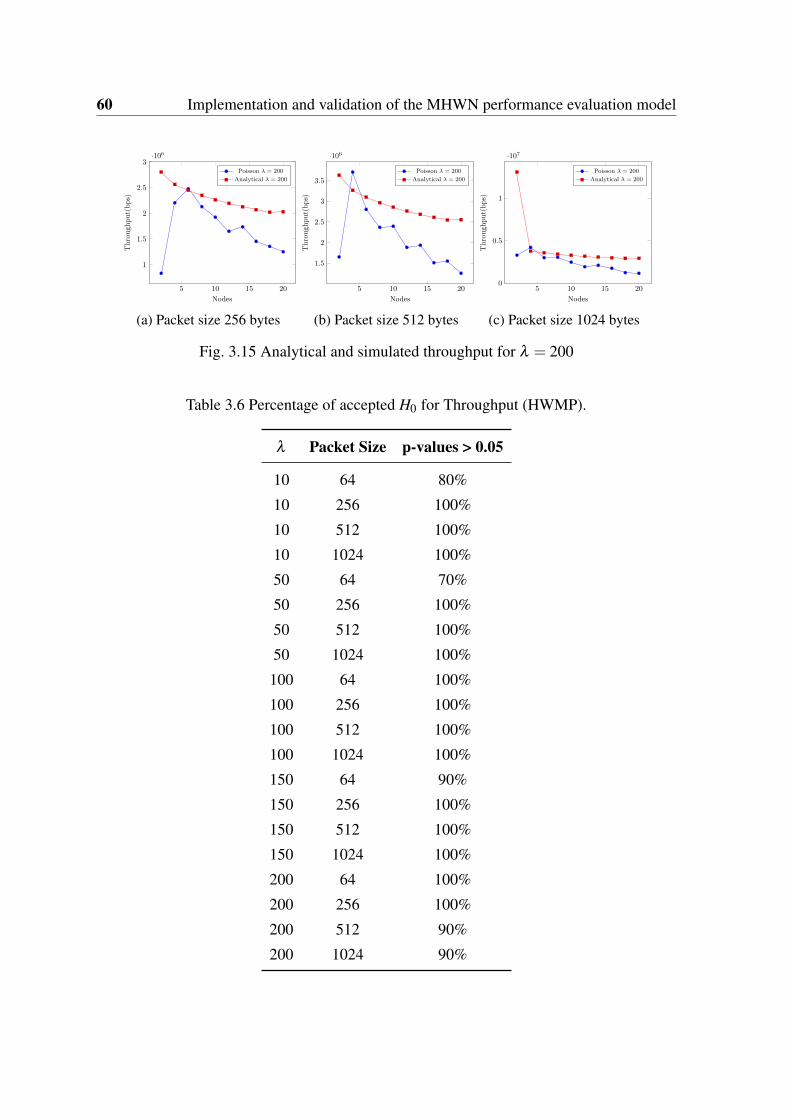
60 Implementation and validation of the MHWN performance evaluation model
5 10 15 20
1
1.5
2
2.5
3·106
Nodes
Through
put(bps)
Poisson λ = 200
Analytical λ = 200
(a) Packet size 256 bytes
5 10 15 20
1.5
2
2.5
3
3.5
·106
NodesThrough
put(bps)
Poisson λ = 200
Analytical λ = 200
(b) Packet size 512 bytes
5 10 15 200
0.5
1
·107
Nodes
Through
put(bps)
Poisson λ = 200
Analytical λ = 200
(c) Packet size 1024 bytes
Fig. 3.15 Analytical and simulated throughput for λ = 200
Table 3.6 Percentage of accepted H0 for Throughput (HWMP).
λ Packet Size p-values > 0.05
10 64 80%
10 256 100%
10 512 100%
10 1024 100%
50 64 70%
50 256 100%
50 512 100%
50 1024 100%
100 64 100%
100 256 100%
100 512 100%
100 1024 100%
150 64 90%
150 256 100%
150 512 100%
150 1024 100%
200 64 100%
200 256 100%
200 512 90%
200 1024 90%
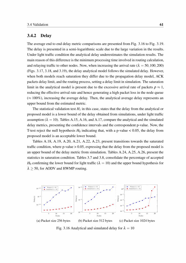
3.4 Validation 61
3.4.2 Delay
The average end to end delay metric comparisons are presented from Fig. 3.16 to Fig. 3.19.The delay is presented in a semi-logarithmic scale due to the large variation in the results.Under light traffic condition the analytical delay underestimates the simulation results. Themain reason of this difference is the minimum processing time involved in routing calculation,and relaying traffic to other nodes. Now, when increasing the arrival rate (λ = 50,100,200)(Figs. 3.17, 3.18, and 3.19), the delay analytical model follows the simulated delay. However,when both models reach saturation they differ due to the propagation delay model, ACKpackets delay limit, and the routing process, setting a delay limit in simulation. The saturationlimit in the analytical model is present due to the excessive arrival rate of packets ρ ≈ 1,reducing the effective arrival rate and hence generating a high packet loss in the node queue(≈ 100%), increasing the average delay. Then, the analytical average delay represents anupper bound from the estimated metric.
The statistical validation test H1 in this case, states that the delay from the analytical orproposed model is a lower bound of the delay obtained from simulations, under light trafficassumption (λ = 10). Tables A.15, A.16, and A.17, compare the analytical and the simulateddelay metrics, presenting the confidence intervals and the correspondent p-value. Now, theT-test reject the null hypothesis H0 indicating that, with a p-value < 0.05, the delay fromproposed model is an acceptable lower bound.
Tables A.18, A.19, A.20, A.21, A.22, A.23, present transitions towards the saturatedtraffic condition, where p-value > 0.05, expressing that the delay from the proposed model isan upper bound of the delay metric from simulation. Tables A.24, A.25, A.26, present thestatistics in saturation condition. Tables 3.7 and 3.8, consolidate the percentage of acceptedH0 confirming the lower bound for light traffic (λ = 10) and the upper bound hypothesis forλ ≥ 50, for AODV and HWMP routing.
5 10 15 20
10−3.5
10−3
10−2.5
Nodes
Delay(s)
Poisson λ = 10
Analytical λ = 10
(a) Packet size 256 bytes
5 10 15 2010−4
10−3
10−2
Nodes
Delay(s)
Poisson λ = 10
Analytical λ = 10
(b) Packet size 512 bytes
5 10 15 20
10−4
10−3
10−2
10−1
100
Nodes
Delay(s)
Poisson λ = 10
Analytical λ = 10
(c) Packet size 1024 bytes
Fig. 3.16 Analytical and simulated delay for λ = 10
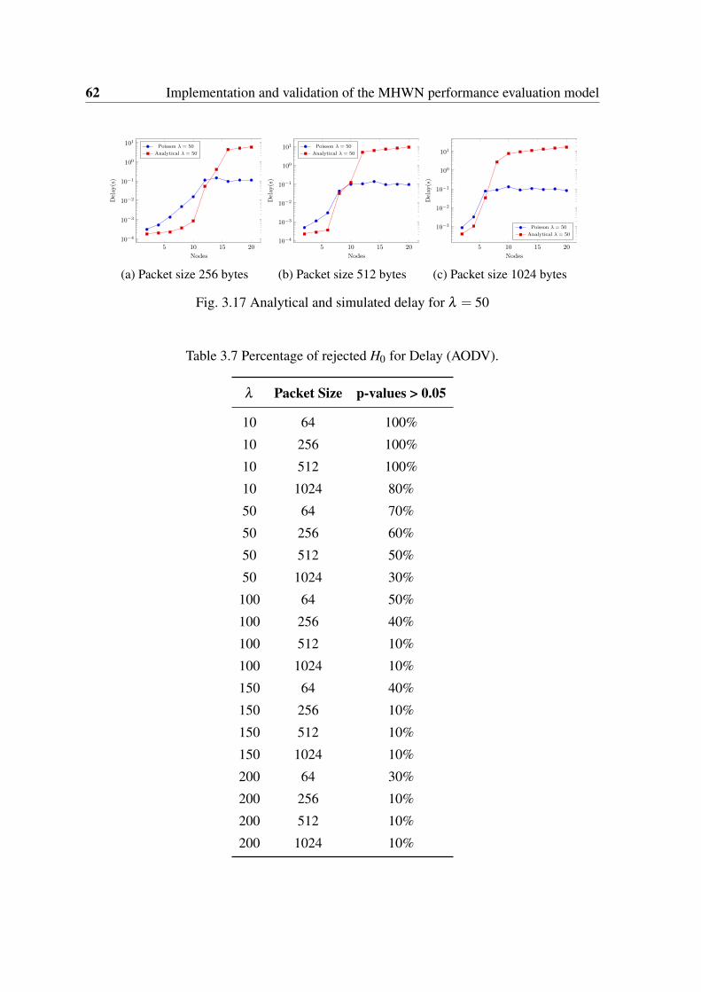
62 Implementation and validation of the MHWN performance evaluation model
5 10 15 2010−4
10−3
10−2
10−1
100
101
Nodes
Delay(s)
Poisson λ = 50
Analytical λ = 50
(a) Packet size 256 bytes
5 10 15 2010−4
10−3
10−2
10−1
100
101
Nodes
Delay(s)
Poisson λ = 50
Analytical λ = 50
(b) Packet size 512 bytes
5 10 15 20
10−3
10−2
10−1
100
101
Nodes
Delay(s)
Poisson λ = 50
Analytical λ = 50
(c) Packet size 1024 bytes
Fig. 3.17 Analytical and simulated delay for λ = 50
Table 3.7 Percentage of rejected H0 for Delay (AODV).
λ Packet Size p-values > 0.05
10 64 100%
10 256 100%
10 512 100%
10 1024 80%
50 64 70%
50 256 60%
50 512 50%
50 1024 30%
100 64 50%
100 256 40%
100 512 10%
100 1024 10%
150 64 40%
150 256 10%
150 512 10%
150 1024 10%
200 64 30%
200 256 10%
200 512 10%
200 1024 10%
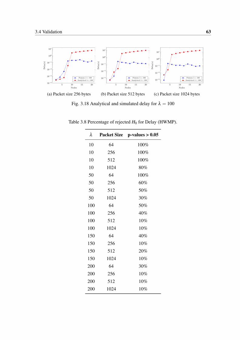
3.4 Validation 63
5 10 15 2010−4
10−3
10−2
10−1
100
101
Nodes
Delay(s)
Poisson λ = 100
Analytical λ = 100
(a) Packet size 256 bytes
5 10 15 20
10−3
10−2
10−1
100
101
Nodes
Delay(s)
Poisson λ = 100
Analytical λ = 100
(b) Packet size 512 bytes
5 10 15 20
10−3
10−2
10−1
100
101
Nodes
Delay(s)
Poisson λ = 100
Analytical λ = 100
(c) Packet size 1024 bytes
Fig. 3.18 Analytical and simulated delay for λ = 100
Table 3.8 Percentage of rejected H0 for Delay (HWMP).
λ Packet Size p-values > 0.05
10 64 100%
10 256 100%
10 512 100%
10 1024 80%
50 64 100%
50 256 60%
50 512 50%
50 1024 30%
100 64 50%
100 256 40%
100 512 10%
100 1024 10%
150 64 40%
150 256 10%
150 512 20%
150 1024 10%
200 64 30%
200 256 10%
200 512 10%
200 1024 10%
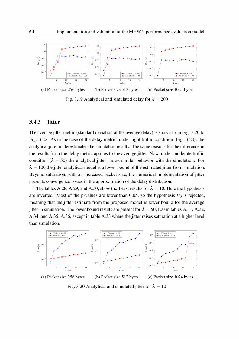
64 Implementation and validation of the MHWN performance evaluation model
5 10 15 20
10−3
10−2
10−1
100
101
Nodes
Delay(s)
Poisson λ = 200
Analytical λ = 200
(a) Packet size 256 bytes
5 10 15 20
10−3
10−2
10−1
100
101
Nodes
Delay(s)
Poisson λ = 200
Analytical λ = 200
(b) Packet size 512 bytes
5 10 15 20
10−3
10−2
10−1
100
101
Nodes
Delay(s)
Poisson λ = 200
Analytical λ = 200
(c) Packet size 1024 bytes
Fig. 3.19 Analytical and simulated delay for λ = 200
3.4.3 Jitter
The average jitter metric (standard deviation of the average delay) is shown from Fig. 3.20 toFig. 3.22. As in the case of the delay metric, under light traffic condition (Fig. 3.20), theanalytical jitter underestimates the simulation results. The same reasons for the difference inthe results from the delay metric applies to the average jitter. Now, under moderate trafficcondition (λ = 50) the analytical jitter shows similar behavior with the simulation. Forλ = 100 the jitter analytical model is a lower bound of the estimated jitter from simulation.Beyond saturation, with an increased packet size, the numerical implementation of jitterpresents convergence issues in the approximation of the delay distribution.
The tables A.28, A.29, and A.30, show the T-test results for λ = 10. Here the hypothesisare inverted. Most of the p-values are lower than 0.05, so the hypothesis H0 is rejected,meaning that the jitter estimate from the proposed model is lower bound for the averagejitter in simulation. The lower bound results are present for λ = 50,100 in tables A.31, A.32,A.34, and A.35, A.36, except in table A.33 where the jitter raises saturation at a higher levelthan simulation.
5 10 15 20
10−4
10−3
Nodes
Jitter(s)
Poisson λ = 10
Analytical λ = 10
(a) Packet size 256 bytes
5 10 15 20
10−4
10−3
10−2
Nodes
Jitter(s)
Poisson λ = 10
Analytical λ = 10
(b) Packet size 512 bytes
5 10 15 2010−4
10−3
10−2
10−1
100
Nodes
Jitter(s)
Poisson λ = 10
Analytical λ = 10
(c) Packet size 1024 bytes
Fig. 3.20 Analytical and simulated jitter for λ = 10
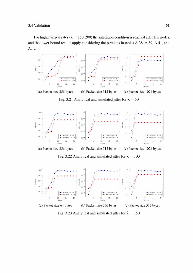
3.4 Validation 65
For higher arrival rates (λ = 150,200) the saturation condition is reached after few nodes,and the lower bound results apply considering the p-values in tables A.38, A.39, A.41, andA.42.
5 10 15 20
10−4
10−3
10−2
10−1
Nodes
Jitter(s)
Poisson λ = 50
Analytical λ = 50
(a) Packet size 256 bytes
5 10 15 20
10−4
10−3
10−2
10−1
Nodes
Jitter(s)
Poisson λ = 50
Analytical λ = 50
(b) Packet size 512 bytes
5 10 15 2010−4
10−3
10−2
10−1
100
Nodes
Jitter(s)
Poisson λ = 50
Analytical λ = 50
(c) Packet size 1024 bytes
Fig. 3.21 Analytical and simulated jitter for λ = 50
5 10 15 20
10−4
10−3
10−2
10−1
100
Nodes
Jitter(s)
Poisson λ = 100
Analytical λ = 100
(a) Packet size 256 bytes
5 10 15 20
10−4
10−3
10−2
10−1
100
Nodes
Jitter(s)
Poisson λ = 100
Analytical λ = 100
(b) Packet size 512 bytes
5 10 15 20
10−3
10−2
10−1
100
Nodes
Jitter(s)
Poisson λ = 100
Analytical λ = 100
(c) Packet size 1024 bytes
Fig. 3.22 Analytical and simulated jitter for λ = 100
5 10 15 20
10−4
10−3
10−2
10−1
100
Nodes
Jitter(s)
Poisson λ = 150
Analytical λ = 150
(a) Packet size 64 bytes
5 10 15 20
10−4
10−3
10−2
10−1
100
Nodes
Jitter(s)
Poisson λ = 150
Analytical λ = 150
(b) Packet size 256 bytes
5 10 15 20
10−4
10−3
10−2
10−1
100
Nodes
Jitter(s)
Poisson λ = 150
Analytical λ = 150
(c) Packet size 512 bytes
Fig. 3.23 Analytical and simulated jitter for λ = 150
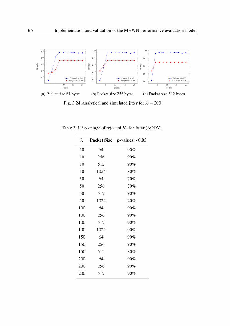
66 Implementation and validation of the MHWN performance evaluation model
5 10 15 20
10−4
10−3
10−2
10−1
100
Nodes
Jitter(s)
Poisson λ = 200
Analytical λ = 200
(a) Packet size 64 bytes
5 10 15 20
10−4
10−3
10−2
10−1
100
NodesJitter(s)
Poisson λ = 200
Analytical λ = 200
(b) Packet size 256 bytes
5 10 15 20
10−4
10−3
10−2
10−1
100
Nodes
Jitter(s)
Poisson λ = 200
Analytical λ = 200
(c) Packet size 512 bytes
Fig. 3.24 Analytical and simulated jitter for λ = 200
Table 3.9 Percentage of rejected H0 for Jitter (AODV).
λ Packet Size p-values > 0.05
10 64 90%
10 256 90%
10 512 90%
10 1024 80%
50 64 70%
50 256 70%
50 512 90%
50 1024 20%
100 64 90%
100 256 90%
100 512 90%
100 1024 90%
150 64 90%
150 256 90%
150 512 80%
200 64 90%
200 256 90%
200 512 90%
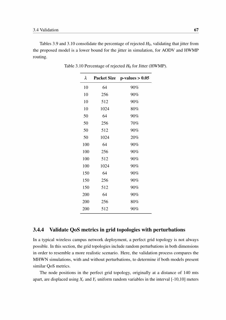
3.4 Validation 67
Tables 3.9 and 3.10 consolidate the percentage of rejected H0, validating that jitter fromthe proposed model is a lower bound for the jitter in simulation, for AODV and HWMProuting.
Table 3.10 Percentage of rejected H0 for Jitter (HWMP).
λ Packet Size p-values > 0.05
10 64 90%
10 256 90%
10 512 90%
10 1024 80%
50 64 90%
50 256 70%
50 512 90%
50 1024 20%
100 64 90%
100 256 90%
100 512 90%
100 1024 90%
150 64 90%
150 256 90%
150 512 90%
200 64 90%
200 256 80%
200 512 90%
3.4.4 Validate QoS metrics in grid topologies with perturbations
In a typical wireless campus network deployment, a perfect grid topology is not alwayspossible. In this section, the grid topologies include random perturbations in both dimensionsin order to resemble a more realistic scenario. Here, the validation process compares theMHWN simulations, with and without perturbations, to determine if both models presentsimilar QoS metrics.
The node positions in the perfect grid topology, originally at a distance of 140 mtsapart, are displaced using Xr and Yr uniform random variables in the interval [-10,10] meters
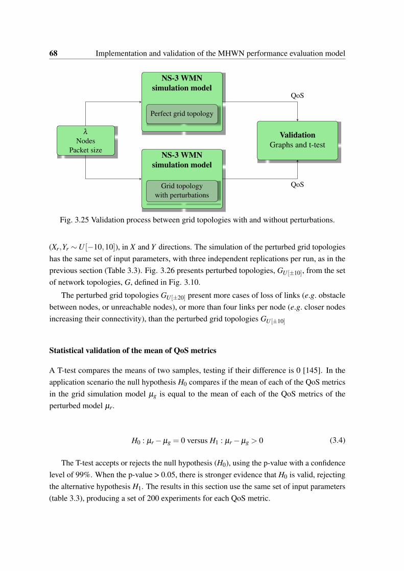
68 Implementation and validation of the MHWN performance evaluation model
NS-3 WMNsimulation model
Perfect grid topology
λ
NodesPacket size NS-3 WMN
simulation model
Grid topologywith perturbations
ValidationGraphs and t-test
QoS
QoS
Fig. 3.25 Validation process between grid topologies with and without perturbations.
(Xr,Yr ∼U [−10,10]), in X and Y directions. The simulation of the perturbed grid topologieshas the same set of input parameters, with three independent replications per run, as in theprevious section (Table 3.3). Fig. 3.26 presents perturbed topologies, GU [±10], from the setof network topologies, G, defined in Fig. 3.10.
The perturbed grid topologies GU [±20] present more cases of loss of links (e.g. obstaclebetween nodes, or unreachable nodes), or more than four links per node (e.g. closer nodesincreasing their connectivity), than the perturbed grid topologies GU [±10]
Statistical validation of the mean of QoS metrics
A T-test compares the means of two samples, testing if their difference is 0 [145]. In theapplication scenario the null hypothesis H0 compares if the mean of each of the QoS metricsin the grid simulation model µg is equal to the mean of each of the QoS metrics of theperturbed model µr.
H0 : µr−µg = 0 versus H1 : µr−µg > 0 (3.4)
The T-test accepts or rejects the null hypothesis (H0), using the p-value with a confidencelevel of 99%. When the p-value > 0.05, there is stronger evidence that H0 is valid, rejectingthe alternative hypothesis H1. The results in this section use the same set of input parameters(table 3.3), producing a set of 200 experiments for each QoS metric.
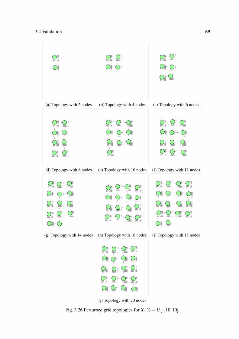
3.4 Validation 69
(a) Topology with 2 nodes (b) Topology with 4 nodes (c) Topology with 6 nodes
(d) Topology with 8 nodes (e) Topology with 10 nodes (f) Topology with 12 nodes
(g) Topology with 14 nodes (h) Topology with 16 nodes (i) Topology with 18 nodes
(j) Topology with 20 nodes
Fig. 3.26 Perturbed grid topologies for Xr,Yr ∼U [−10,10].
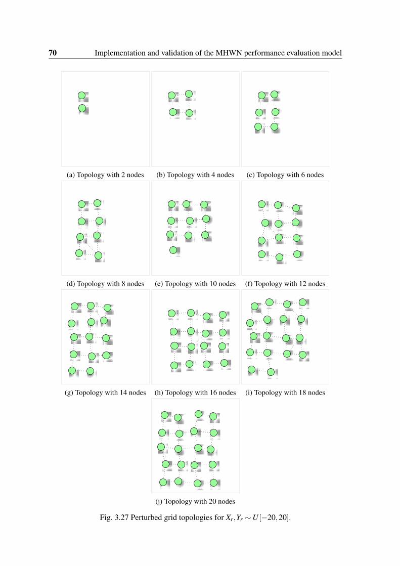
70 Implementation and validation of the MHWN performance evaluation model
(a) Topology with 2 nodes (b) Topology with 4 nodes (c) Topology with 6 nodes
(d) Topology with 8 nodes (e) Topology with 10 nodes (f) Topology with 12 nodes
(g) Topology with 14 nodes (h) Topology with 16 nodes (i) Topology with 18 nodes
(j) Topology with 20 nodes
Fig. 3.27 Perturbed grid topologies for Xr,Yr ∼U [−20,20].
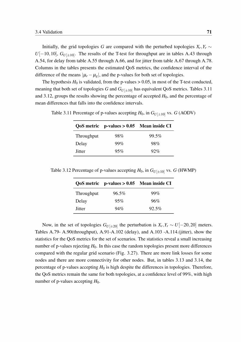
3.4 Validation 71
Initially, the grid topologies G are compared with the perturbed topologies Xr,Yr ∼U [−10,10], GU [±10]. The results of the T-test for throughput are in tables A.43 throughA.54, for delay from table A.55 through A.66, and for jitter from table A.67 through A.78.Columns in the tables presents the estimated QoS metrics, the confidence interval of thedifference of the means |µr−µg|, and the p-values for both set of topologies.
The hypothesis H0 is validated, from the p-values > 0.05, in most of the T-test conducted,meaning that both set of topologies G and GU [±10] has equivalent QoS metrics. Tables 3.11and 3.12, groups the results showing the percentage of accepted H0, and the percentage ofmean differences that falls into the confidence intervals.
Table 3.11 Percentage of p-values accepting H0, in GU [±10] vs. G (AODV)
QoS metric p-values > 0.05 Mean inside CI
Throughput 98% 99.5%
Delay 99% 98%
Jitter 95% 92%
Table 3.12 Percentage of p-values accepting H0, in GU [±10] vs. G (HWMP)
QoS metric p-values > 0.05 Mean inside CI
Throughput 96.5% 99%
Delay 95% 96%
Jitter 94% 92.5%
Now, in the set of topologies GU [±20] the perturbation is Xr,Yr ∼ U [−20,20] meters.Tables A.79- A.90(throughput), A.91-A.102 (delay), and A.103 -A.114.(jitter), show thestatistics for the QoS metrics for the set of scenarios. The statistics reveal a small increasingnumber of p-values rejecting H0. In this case the random topologies present more differencescompared with the regular grid scenario (Fig. 3.27). There are more link losses for somenodes and there are more connectivity for other nodes. But, in tables 3.13 and 3.14, thepercentage of p-values accepting H0 is high despite the differences in topologies. Therefore,the QoS metrics remain the same for both topologies, at a confidence level of 99%, with highnumber of p-values accepting H0.
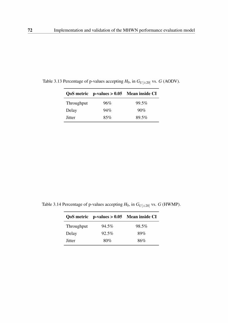
72 Implementation and validation of the MHWN performance evaluation model
Table 3.13 Percentage of p-values accepting H0, in GU [±20] vs. G (AODV).
QoS metric p-values > 0.05 Mean inside CI
Throughput 96% 99.5%
Delay 94% 90%
Jitter 85% 89.5%
Table 3.14 Percentage of p-values accepting H0, in GU [±20] vs. G (HWMP).
QoS metric p-values > 0.05 Mean inside CI
Throughput 94.5% 98.5%
Delay 92.5% 89%
Jitter 80% 86%
3.5 Conclusions 73
3.5 Conclusions
In this chapter, the algorithms of the MHWN performance evaluation model are implementedin Python. This programming language provides a wide range of open source libraries,required in the implementation process. Based on the available libraries, a hierarchical sourcecode was constructed.
Effective routines in the source code were implemented, like the PGF inversion andLaplace transform inversion, using the appropriate numerical solutions. Such routinespresent high speed of convergence, thanks to the IFFT involved in the process. Therefore,the computational time is reduced to less than three minutes, when using the set of inputparameters described before. This is an advantage against the computational time requiredby the simulation model.
In this work, the analytical or performance model is compared with a simulation modelavailable in NS-3, not with a custom discrete event simulation resembling the simplifiedstochastic process. The NS-3 simulation model includes a full set of configurable features, ateach network layer. The physical layer implements a channel model with delay propagationand loss propagation. Other settings involves the transmission power and energy detectionthreshold. The MAC layer include the 802.11 standard and the mesh implementation,where the path selection or routing protocol present several settings. In this work, the NS-3simulation model is updated, developing the code for a Poisson packet generator to validatethe arrival traffic assumption in the proposed performance model. Also, the simulationgenerates a set of traces required to extract the QoS metrics. The set of traces is generated bycreating a mesh packet dissector, not available in NS-3. The validation presents satisfactoryresults estimating the QoS metrics. From visual inspection the saturation point, or the stepchange in QoS metrics, is accurately estimated. Most of the validation process related withperformance models, found in the literature, present visual or graphical results. In this work afull set of statistical procedures is developed to test the validity of the QoS metrics estimation.The hypothesis tests compare the QoS metrics from the proposed MHWN performancemodel and the NS-3 simulation model.
From the number p-values accepting the hypothesis, resulting from the T-tests statistics,the throughput from the proposed model is at least an upper bound estimate for AODV in98% of the simulations, and for HWMP in 97% of the simulations. The delay and jitteranalytical estimates from the proposed MHWN model, can be also used as lower or upperbounds depending on the traffic condition. In case of the delay, for low arrival rate (λ = 10),the estimate from the proposed model is a lower bound in 95% of the cases, for AODV andHWMP. Now, increasing the arrival rate, the hypothesis is rejected and the delay becomes anupper bound in 71.8% of the cases, for AODV, and 75.6% of the cases, for HWMP. The jitter
74 Implementation and validation of the MHWN performance evaluation model
metric from the proposed model is a lower bound of the simulation model in 84.5% and 85.5%of the cases, for AODV and HWMP respectively. The delay and jitter metric estimates differdue to the complexity presented in the NS-3 simulation model. Features like propagationdelay and loss model, ACK packets delay limit, and delay limit in routing process, affectthe packet’s delay in simulation. These results are promising considering the complexityassociated in the transmission process developed in the NS-3 simulator. Further research isrequired to obtain closer estimates to simulation, and with the appropriate extensions to themodel, it could improve the presented results.
The MHWN application scenario presents regular grid topologies, considering samedistance between nodes and four neighbors per node. This node distribution is valid interms of coverage area and node density. Assuming a more realistic approach, another set ofhypothesis testing is conducted comparing regular and perturbed grid topologies, in orderto assess the equivalence in the QoS metrics. In this case, the T-tests statistics reveal thatthe QoS metrics remain equivalent, with a high number of p-values and confidence intervalsaccepting the hypothesis, 93% on average. Despite of random displacement of nodes, thisresults validate regular grid topologies in the application scenario.
The proposed MHWN model can be easily adapted to other protocols like 802.11b or802.11g, or it can be modified to resemble other contention access methods like implementedin WSNs or VANETs.
Chapter 4
Performance evaluation model:validation in the application scenario
4.1 Introduction
Peer-to-Peer (P2P) video streaming features low server infrastructure cost and good scala-bility, and has recently been used as an alternative to traditional streaming services. Suchstreaming applications have become very accessible, thanks to the wireless network interfaceavailable in a wide number of electronic devices. Typical P2P streaming services like P2PTV,video-conference, and live streaming, can be deployed over multihop wireless local areanetworks (MHWN).
In this chapter, the performance evaluation model is validated against an emulation model.In the emulation model a real-time P2P streaming application transmits to other nodes in theMHWN, resembling an adequate application scenario, like e-learning in a campus network.The emulation process uses the same simulation testbed of a WMN, as in the previous chapterforming a regular grid topology, but this time there is a real application generating traffic.This is accomplished enabling the emulation mode available in NS-3 simulator, and runninga P2P-TV application over Linux Containers (LXC) (Fig. 3.2).
Initially we present the analytical model assumptions related to the P2P streamingapplication. Then, we validate the Poisson assumption applied to the streaming video. Theperformance metrics from the MAC model are calculated, and they are validated with theNS-3 experimental testbed in the results section.
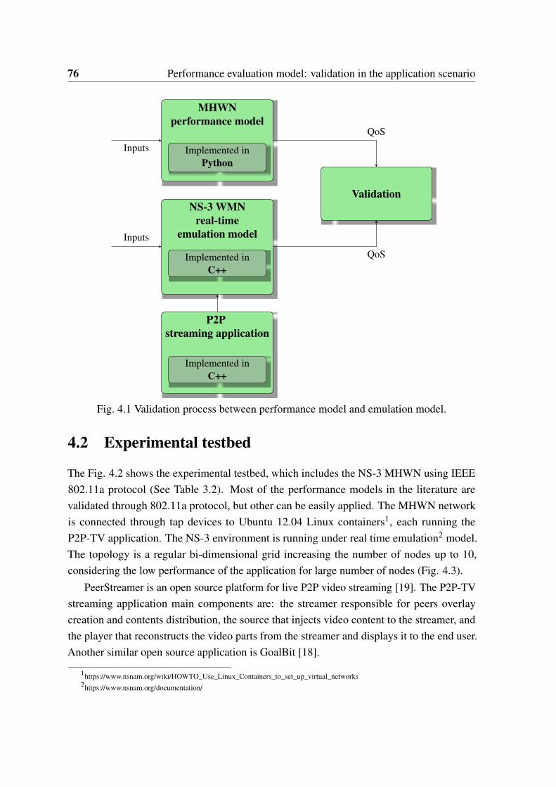
76 Performance evaluation model: validation in the application scenario
MHWNperformance model
Implemented inPython
Inputs
NS-3 WMNreal-time
emulation model
Implemented inC++
Inputs
P2Pstreaming application
Implemented inC++
Validation
QoS
QoS
Fig. 4.1 Validation process between performance model and emulation model.
4.2 Experimental testbed
The Fig. 4.2 shows the experimental testbed, which includes the NS-3 MHWN using IEEE802.11a protocol (See Table 3.2). Most of the performance models in the literature arevalidated through 802.11a protocol, but other can be easily applied. The MHWN networkis connected through tap devices to Ubuntu 12.04 Linux containers1, each running theP2P-TV application. The NS-3 environment is running under real time emulation2 model.The topology is a regular bi-dimensional grid increasing the number of nodes up to 10,considering the low performance of the application for large number of nodes (Fig. 4.3).
PeerStreamer is an open source platform for live P2P video streaming [19]. The P2P-TVstreaming application main components are: the streamer responsible for peers overlaycreation and contents distribution, the source that injects video content to the streamer, andthe player that reconstructs the video parts from the streamer and displays it to the end user.Another similar open source application is GoalBit [18].
1https://www.nsnam.org/wiki/HOWTO_Use_Linux_Containers_to_set_up_virtual_networks2https://www.nsnam.org/documentation/
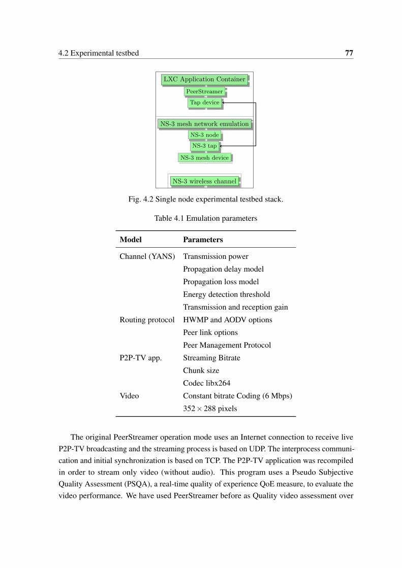
4.2 Experimental testbed 77
LXC Application Container
PeerStreamer
Tap device
NS-3 mesh network emulation
NS-3 node
NS-3 tap
NS-3 mesh device
NS-3 wireless channel
Fig. 4.2 Single node experimental testbed stack.
Table 4.1 Emulation parameters
Model Parameters
Channel (YANS) Transmission power
Propagation delay model
Propagation loss model
Energy detection threshold
Transmission and reception gain
Routing protocol HWMP and AODV options
Peer link options
Peer Management Protocol
P2P-TV app. Streaming Bitrate
Chunk size
Codec libx264
Video Constant bitrate Coding (6 Mbps)
352×288 pixels
The original PeerStreamer operation mode uses an Internet connection to receive liveP2P-TV broadcasting and the streaming process is based on UDP. The interprocess communi-cation and initial synchronization is based on TCP. The P2P-TV application was recompiledin order to stream only video (without audio). This program uses a Pseudo SubjectiveQuality Assessment (PSQA), a real-time quality of experience QoE measure, to evaluate thevideo performance. We have used PeerStreamer before as Quality video assessment over
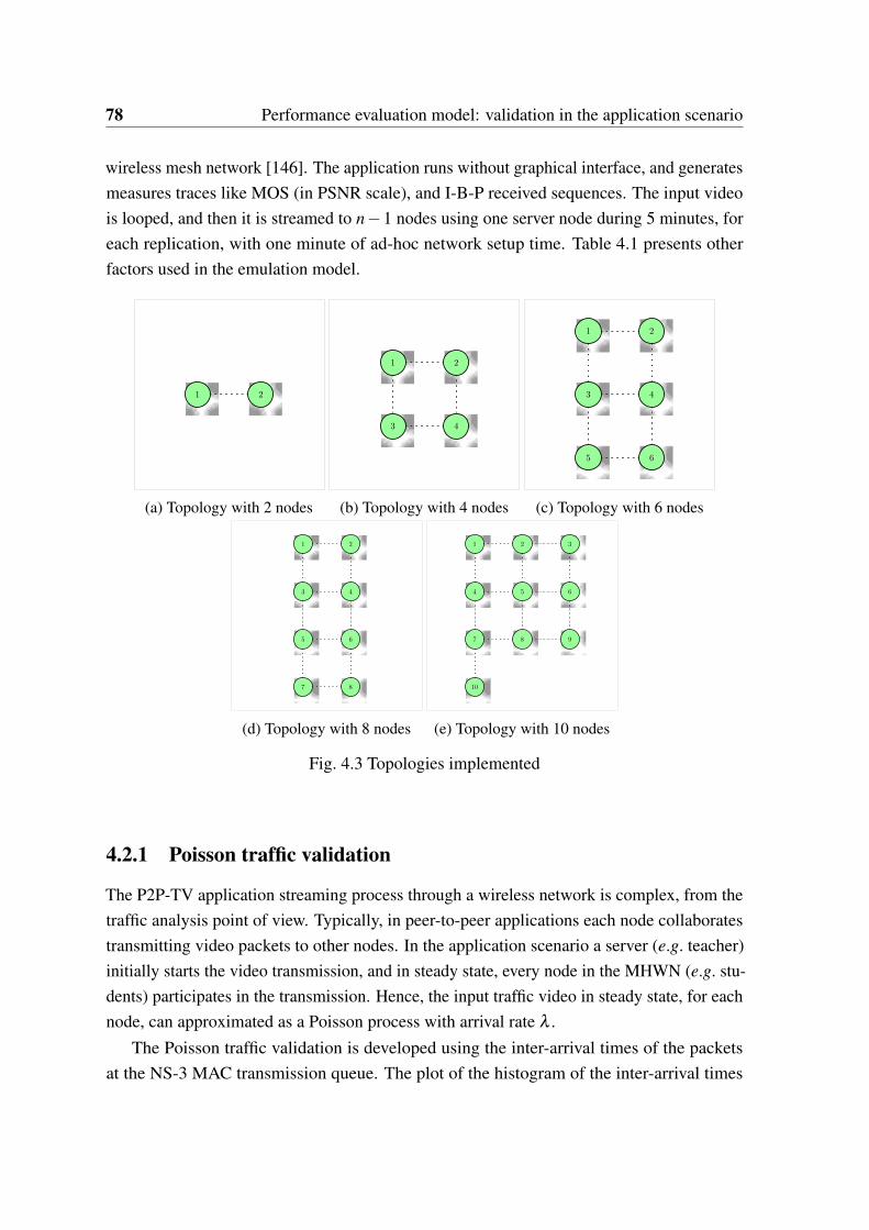
78 Performance evaluation model: validation in the application scenario
wireless mesh network [146]. The application runs without graphical interface, and generatesmeasures traces like MOS (in PSNR scale), and I-B-P received sequences. The input videois looped, and then it is streamed to n−1 nodes using one server node during 5 minutes, foreach replication, with one minute of ad-hoc network setup time. Table 4.1 presents otherfactors used in the emulation model.
1 2
(a) Topology with 2 nodes
1 2
3 4
(b) Topology with 4 nodes
1 2
3 4
5 6
(c) Topology with 6 nodes
1 2
3 4
5 6
7 8
(d) Topology with 8 nodes
1 2 3
4 5 6
7 8 9
10
(e) Topology with 10 nodes
Fig. 4.3 Topologies implemented
4.2.1 Poisson traffic validation
The P2P-TV application streaming process through a wireless network is complex, from thetraffic analysis point of view. Typically, in peer-to-peer applications each node collaboratestransmitting video packets to other nodes. In the application scenario a server (e.g. teacher)initially starts the video transmission, and in steady state, every node in the MHWN (e.g. stu-dents) participates in the transmission. Hence, the input traffic video in steady state, for eachnode, can approximated as a Poisson process with arrival rate λ .
The Poisson traffic validation is developed using the inter-arrival times of the packetsat the NS-3 MAC transmission queue. The plot of the histogram of the inter-arrival times
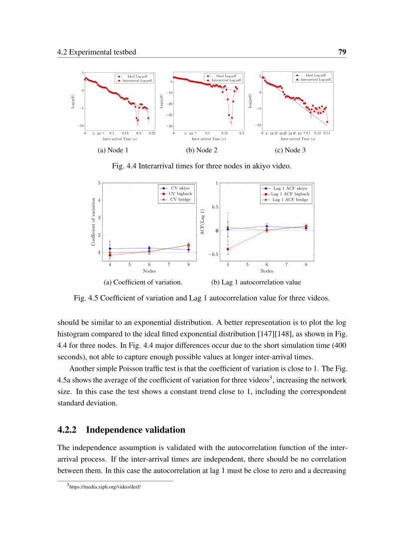
4.2 Experimental testbed 79
0 5 · 10−2 0.1 0.15 0.2 0.25
−10
−5
0
5
Inter-arrival Time (s)
Log
(pdf)
Ideal Log-pdf
Interarrival Log-pdf
(a) Node 1
0 5 · 10−2 0.1 0.15 0.2
−40
−30
−20
−10
0
Inter-arrival Time (s)
Log(pdf)
Ideal Log-pdf
Interarrival Log-pdf
(b) Node 2
0 2 · 10−24 · 10−26 · 10−28 · 10−2 0.1 0.12 0.14
−10
−5
0
5
Inter-arrival Time (s)
Log(pdf)
Ideal Log-pdf
Interarrival Log-pdf
(c) Node 3
Fig. 4.4 Interarrival times for three nodes in akiyo video.
4 5 6 7 8
1
2
3
4
5
1
Nodes
Coeffi
cien
tof
vari
atio
n
CV akiyo
CV bigbuck
CV bridge
(a) Coefficient of variation.
4 5 6 7 8
−0.5
0
0.5
1
0
Nodes
ACF(L
ag1)
Lag 1 ACF akiyo
Lag 1 ACF bigbuck
Lag 1 ACF bridge
(b) Lag 1 autocorrelation value
Fig. 4.5 Coefficient of variation and Lag 1 autocorrelation value for three videos.
should be similar to an exponential distribution. A better representation is to plot the loghistogram compared to the ideal fitted exponential distribution [147][148], as shown in Fig.4.4 for three nodes. In Fig. 4.4 major differences occur due to the short simulation time (400seconds), not able to capture enough possible values at longer inter-arrival times.
Another simple Poisson traffic test is that the coefficient of variation is close to 1. The Fig.4.5a shows the average of the coefficient of variation for three videos3, increasing the networksize. In this case the test shows a constant trend close to 1, including the correspondentstandard deviation.
4.2.2 Independence validation
The independence assumption is validated with the autocorrelation function of the inter-arrival process. If the inter-arrival times are independent, there should be no correlationbetween them. In this case the autocorrelation at lag 1 must be close to zero and a decreasing
3https://media.xiph.org/video/derf/
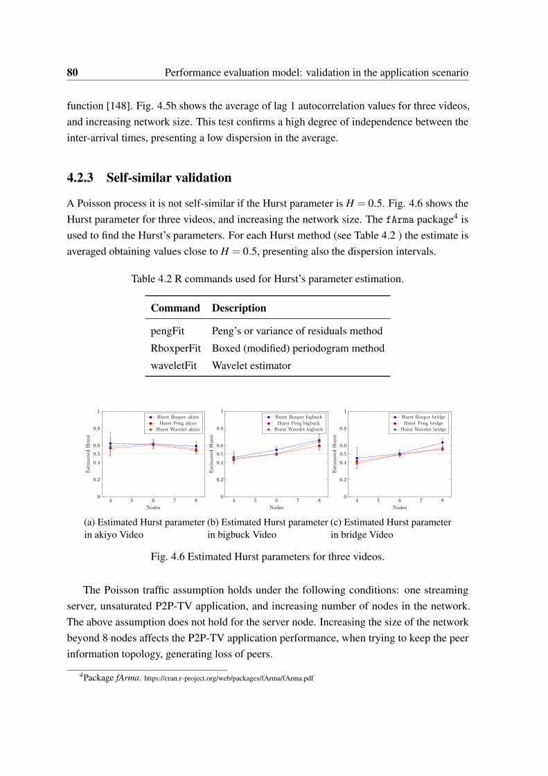
80 Performance evaluation model: validation in the application scenario
function [148]. Fig. 4.5b shows the average of lag 1 autocorrelation values for three videos,and increasing network size. This test confirms a high degree of independence between theinter-arrival times, presenting a low dispersion in the average.
4.2.3 Self-similar validation
A Poisson process it is not self-similar if the Hurst parameter is H = 0.5. Fig. 4.6 shows theHurst parameter for three videos, and increasing the network size. The fArma package4 isused to find the Hurst’s parameters. For each Hurst method (see Table 4.2 ) the estimate isaveraged obtaining values close to H = 0.5, presenting also the dispersion intervals.
Table 4.2 R commands used for Hurst’s parameter estimation.
Command Description
pengFit Peng’s or variance of residuals method
RboxperFit Boxed (modified) periodogram method
waveletFit Wavelet estimator
4 5 6 7 80
0.2
0.4
0.6
0.8
1
0.5
Nodes
Estim
ated
Hurst
Hurst Boxper akiyo
Hurst Peng akiyo
Hurst Wavelet akiyo
(a) Estimated Hurst parameterin akiyo Video
4 5 6 7 80
0.2
0.4
0.6
0.8
1
0.5
Nodes
Estim
ated
Hurst
Hurst Boxper bigbuck
Hurst Peng bigbuck
Hurst Wavelet bigbuck
(b) Estimated Hurst parameterin bigbuck Video
4 5 6 7 80
0.2
0.4
0.6
0.8
1
0.5
Nodes
Estim
ated
Hurst
Hurst Boxper bridge
Hurst Peng bridge
Hurst Wavelet bridge
(c) Estimated Hurst parameterin bridge Video
Fig. 4.6 Estimated Hurst parameters for three videos.
The Poisson traffic assumption holds under the following conditions: one streamingserver, unsaturated P2P-TV application, and increasing number of nodes in the network.The above assumption does not hold for the server node. Increasing the size of the networkbeyond 8 nodes affects the P2P-TV application performance, when trying to keep the peerinformation topology, generating loss of peers.
4Package fArma. https://cran.r-project.org/web/packages/fArma/fArma.pdf

4.3 Validation 81
4.3 Validation
The set of results is obtained by averaging three independent random runs, per emulationparameters, with the appropriate settings in the NS-3 environment. The set of variableemulation parameters (Table 4.3) covers different topologies, videos5, and bitrates. Todevelop a reliable emulation, the difference between real-time clock and emulation clockmust be close to cero. Hence, the NS-3 is compiled in the optimized mode, and setting theproper available architecture (corei7-avx).
Table 4.3 Set of variable emulation parameters
Parameter Values
Nodes [2,4,6,8,10]
Bitrate(Mbps) [0.1,0.5,1,1.5]
Routing AODV, HWMP
Distance 140m
Videos akiyo, foreman, highway,
bigbuckbunny, bridge-close
The P2P-TV application streams a video trying to keep the specified bitrate, implementinga variable arrival rate and variable packet size. In order to compare the emulation results withthe analytical estimates, the average arrival rate and the average packet size generated in theemulation process, were used as the input in the analytical model.
(a) Akiyo. (b) Foreman. (c) Bridge close.
(d) Highway. (e) Big Buck Bunny
Fig. 4.7 Selected videos for real-time emulation.
5https://media.xiph.org/video/derf/
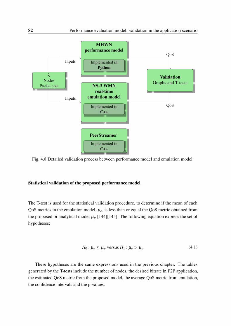
82 Performance evaluation model: validation in the application scenario
MHWNperformance model
Implemented inPython
Inputs
NS-3 WMNreal-time
emulation model
Implemented inC++
λ
NodesPacket size
Inputs
PeerStreamer
Implemented inC++
ValidationGraphs and T-tests
QoS
QoS
Fig. 4.8 Detailed validation process between performance model and emulation model.
Statistical validation of the proposed performance model
The T-test is used for the statistical validation procedure, to determine if the mean of eachQoS metrics in the emulation model, µe, is less than or equal the QoS metric obtained fromthe proposed or analytical model µp [144][145]. The following equation express the set ofhypotheses:
H0 : µe ≤ µp versus H1 : µe > µp (4.1)
These hypotheses are the same expressions used in the previous chapter. The tablesgenerated by the T-tests include the number of nodes, the desired bitrate in P2P application,the estimated QoS metric from the proposed model, the average QoS metric from emulation,the confidence intervals and the p-values.
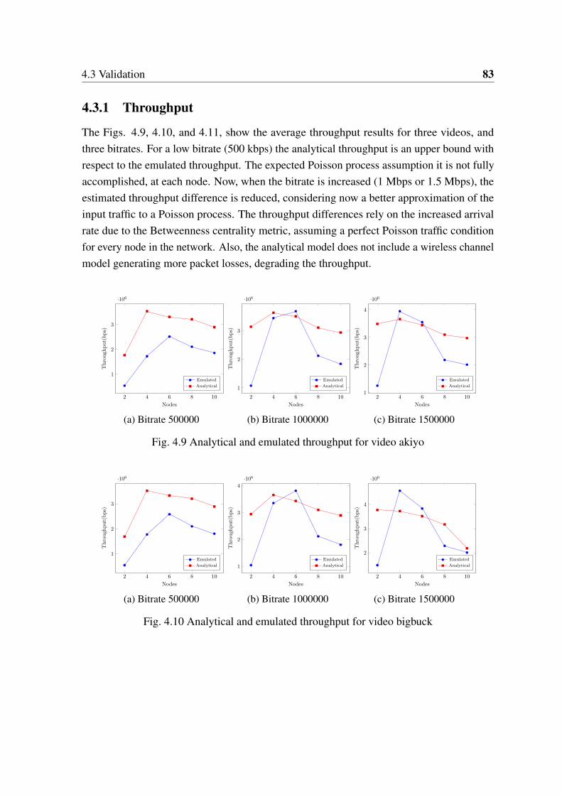
4.3 Validation 83
4.3.1 Throughput
The Figs. 4.9, 4.10, and 4.11, show the average throughput results for three videos, andthree bitrates. For a low bitrate (500 kbps) the analytical throughput is an upper bound withrespect to the emulated throughput. The expected Poisson process assumption it is not fullyaccomplished, at each node. Now, when the bitrate is increased (1 Mbps or 1.5 Mbps), theestimated throughput difference is reduced, considering now a better approximation of theinput traffic to a Poisson process. The throughput differences rely on the increased arrivalrate due to the Betweenness centrality metric, assuming a perfect Poisson traffic conditionfor every node in the network. Also, the analytical model does not include a wireless channelmodel generating more packet losses, degrading the throughput.
2 4 6 8 10
1
2
3
·106
Nodes
Through
put(bps)
Emulated
Analytical
(a) Bitrate 500000
2 4 6 8 10
1
2
3
·106
Nodes
Through
put(bps)
Emulated
Analytical
(b) Bitrate 1000000
2 4 6 8 101
2
3
4
·106
Nodes
Through
put(bps)
Emulated
Analytical
(c) Bitrate 1500000
Fig. 4.9 Analytical and emulated throughput for video akiyo
2 4 6 8 10
1
2
3
·106
Nodes
Through
put(bps)
Emulated
Analytical
(a) Bitrate 500000
2 4 6 8 10
1
2
3
4
·106
Nodes
Through
put(bps)
Emulated
Analytical
(b) Bitrate 1000000
2 4 6 8 10
2
3
4
·106
Nodes
Through
put(bps)
Emulated
Analytical
(c) Bitrate 1500000
Fig. 4.10 Analytical and emulated throughput for video bigbuck
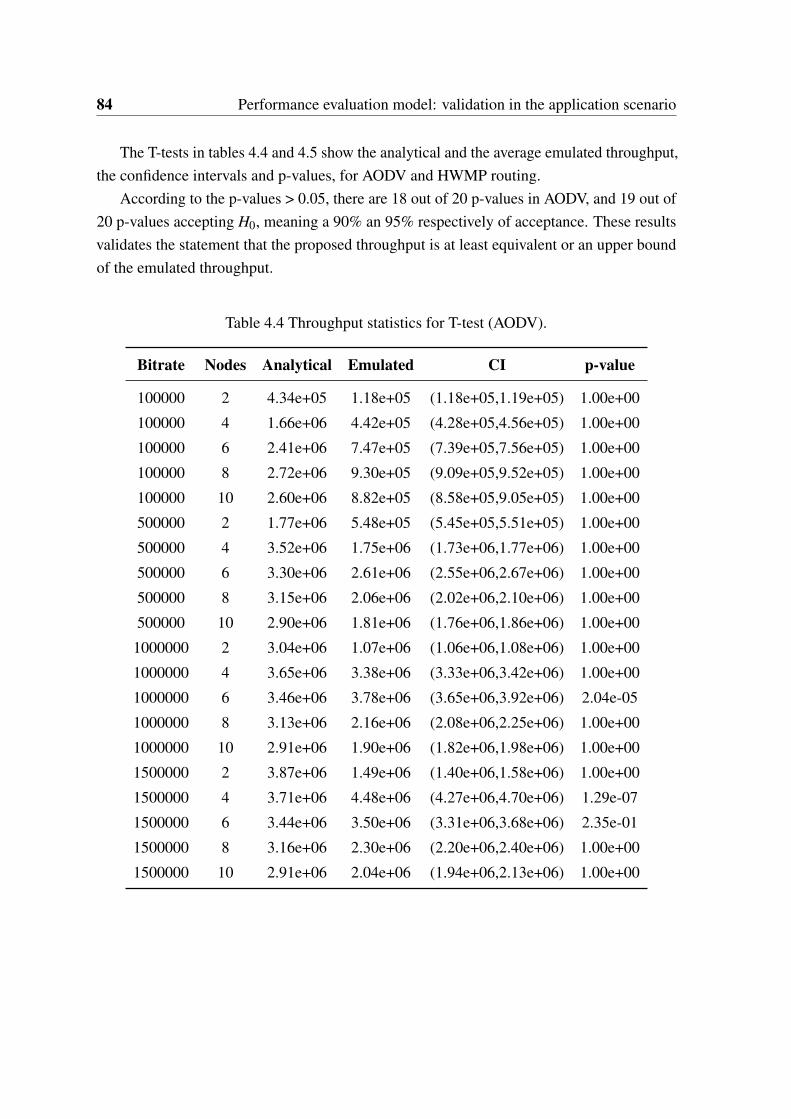
84 Performance evaluation model: validation in the application scenario
The T-tests in tables 4.4 and 4.5 show the analytical and the average emulated throughput,the confidence intervals and p-values, for AODV and HWMP routing.
According to the p-values > 0.05, there are 18 out of 20 p-values in AODV, and 19 out of20 p-values accepting H0, meaning a 90% an 95% respectively of acceptance. These resultsvalidates the statement that the proposed throughput is at least equivalent or an upper boundof the emulated throughput.
Table 4.4 Throughput statistics for T-test (AODV).
Bitrate Nodes Analytical Emulated CI p-value
100000 2 4.34e+05 1.18e+05 (1.18e+05,1.19e+05) 1.00e+00
100000 4 1.66e+06 4.42e+05 (4.28e+05,4.56e+05) 1.00e+00
100000 6 2.41e+06 7.47e+05 (7.39e+05,7.56e+05) 1.00e+00
100000 8 2.72e+06 9.30e+05 (9.09e+05,9.52e+05) 1.00e+00
100000 10 2.60e+06 8.82e+05 (8.58e+05,9.05e+05) 1.00e+00
500000 2 1.77e+06 5.48e+05 (5.45e+05,5.51e+05) 1.00e+00
500000 4 3.52e+06 1.75e+06 (1.73e+06,1.77e+06) 1.00e+00
500000 6 3.30e+06 2.61e+06 (2.55e+06,2.67e+06) 1.00e+00
500000 8 3.15e+06 2.06e+06 (2.02e+06,2.10e+06) 1.00e+00
500000 10 2.90e+06 1.81e+06 (1.76e+06,1.86e+06) 1.00e+00
1000000 2 3.04e+06 1.07e+06 (1.06e+06,1.08e+06) 1.00e+00
1000000 4 3.65e+06 3.38e+06 (3.33e+06,3.42e+06) 1.00e+00
1000000 6 3.46e+06 3.78e+06 (3.65e+06,3.92e+06) 2.04e-05
1000000 8 3.13e+06 2.16e+06 (2.08e+06,2.25e+06) 1.00e+00
1000000 10 2.91e+06 1.90e+06 (1.82e+06,1.98e+06) 1.00e+00
1500000 2 3.87e+06 1.49e+06 (1.40e+06,1.58e+06) 1.00e+00
1500000 4 3.71e+06 4.48e+06 (4.27e+06,4.70e+06) 1.29e-07
1500000 6 3.44e+06 3.50e+06 (3.31e+06,3.68e+06) 2.35e-01
1500000 8 3.16e+06 2.30e+06 (2.20e+06,2.40e+06) 1.00e+00
1500000 10 2.91e+06 2.04e+06 (1.94e+06,2.13e+06) 1.00e+00
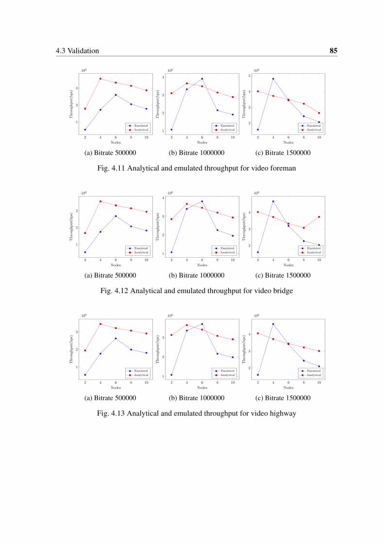
4.3 Validation 85
2 4 6 8 10
1
2
3
·106
Nodes
Through
put(bps)
Emulated
Analytical
(a) Bitrate 500000
2 4 6 8 10
1
2
3
4
·106
Nodes
Through
put(bps)
Emulated
Analytical
(b) Bitrate 1000000
2 4 6 8 10
2
3
4
5
·106
Nodes
Through
put(bps)
Emulated
Analytical
(c) Bitrate 1500000
Fig. 4.11 Analytical and emulated throughput for video foreman
2 4 6 8 10
1
2
3
·106
Nodes
Through
put(bps)
Emulated
Analytical
(a) Bitrate 500000
2 4 6 8 10
1
2
3
4·106
Nodes
Through
put(bps)
Emulated
Analytical
(b) Bitrate 1000000
2 4 6 8 10
2
3
4
·106
Nodes
Through
put(bps)
Emulated
Analytical
(c) Bitrate 1500000
Fig. 4.12 Analytical and emulated throughput for video bridge
2 4 6 8 10
1
2
3
·106
Nodes
Through
put(bps)
Emulated
Analytical
(a) Bitrate 500000
2 4 6 8 10
1
2
3
·106
Nodes
Through
put(bps)
Emulated
Analytical
(b) Bitrate 1000000
2 4 6 8 10
2
3
4
·106
Nodes
Through
put(bps)
Emulated
Analytical
(c) Bitrate 1500000
Fig. 4.13 Analytical and emulated throughput for video highway
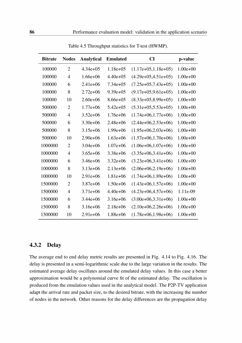
86 Performance evaluation model: validation in the application scenario
Table 4.5 Throughput statistics for T-test (HWMP).
Bitrate Nodes Analytical Emulated CI p-value
100000 2 4.34e+05 1.18e+05 (1.17e+05,1.18e+05) 1.00e+00
100000 4 1.66e+06 4.40e+05 (4.29e+05,4.51e+05) 1.00e+00
100000 6 2.41e+06 7.34e+05 (7.25e+05,7.43e+05) 1.00e+00
100000 8 2.72e+06 9.39e+05 (9.17e+05,9.61e+05) 1.00e+00
100000 10 2.60e+06 8.66e+05 (8.33e+05,8.99e+05) 1.00e+00
500000 2 1.77e+06 5.42e+05 (5.31e+05,5.53e+05) 1.00e+00
500000 4 3.52e+06 1.76e+06 (1.74e+06,1.77e+06) 1.00e+00
500000 6 3.30e+06 2.48e+06 (2.44e+06,2.53e+06) 1.00e+00
500000 8 3.15e+06 1.99e+06 (1.95e+06,2.03e+06) 1.00e+00
500000 10 2.90e+06 1.63e+06 (1.57e+06,1.70e+06) 1.00e+00
1000000 2 3.04e+06 1.07e+06 (1.06e+06,1.07e+06) 1.00e+00
1000000 4 3.65e+06 3.38e+06 (3.35e+06,3.41e+06) 1.00e+00
1000000 6 3.46e+06 3.32e+06 (3.23e+06,3.41e+06) 1.00e+00
1000000 8 3.13e+06 2.13e+06 (2.06e+06,2.19e+06) 1.00e+00
1000000 10 2.91e+06 1.81e+06 (1.74e+06,1.89e+06) 1.00e+00
1500000 2 3.87e+06 1.50e+06 (1.43e+06,1.57e+06) 1.00e+00
1500000 4 3.71e+06 4.40e+06 (4.23e+06,4.57e+06) 1.11e-09
1500000 6 3.44e+06 3.16e+06 (3.00e+06,3.31e+06) 1.00e+00
1500000 8 3.16e+06 2.18e+06 (2.10e+06,2.26e+06) 1.00e+00
1500000 10 2.91e+06 1.88e+06 (1.78e+06,1.98e+06) 1.00e+00
4.3.2 Delay
The average end to end delay metric results are presented in Fig. 4.14 to Fig. 4.16. Thedelay is presented in a semi-logarithmic scale due to the large variation in the results. Theestimated average delay oscillates around the emulated delay values. In this case a betterapproximation would be a polynomial curve fit of the estimated delay. The oscillation isproduced from the emulation values used in the analytical model. The P2P-TV applicationadapt the arrival rate and packet size, to the desired bitrate, with the increasing the numberof nodes in the network. Other reasons for the delay differences are the propagation delay
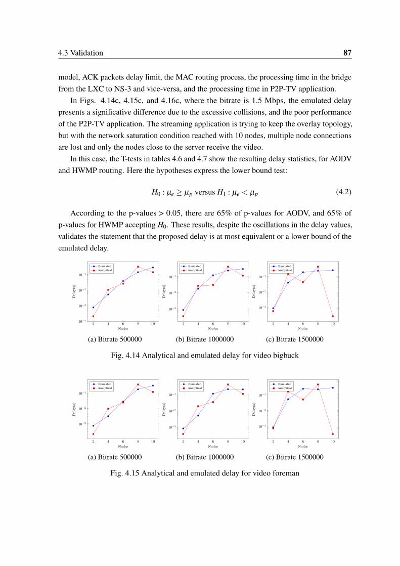
4.3 Validation 87
model, ACK packets delay limit, the MAC routing process, the processing time in the bridgefrom the LXC to NS-3 and vice-versa, and the processing time in P2P-TV application.
In Figs. 4.14c, 4.15c, and 4.16c, where the bitrate is 1.5 Mbps, the emulated delaypresents a significative difference due to the excessive collisions, and the poor performanceof the P2P-TV application. The streaming application is trying to keep the overlay topology,but with the network saturation condition reached with 10 nodes, multiple node connectionsare lost and only the nodes close to the server receive the video.
In this case, the T-tests in tables 4.6 and 4.7 show the resulting delay statistics, for AODVand HWMP routing. Here the hypotheses express the lower bound test:
H0 : µe ≥ µp versus H1 : µe < µp (4.2)
According to the p-values > 0.05, there are 65% of p-values for AODV, and 65% ofp-values for HWMP accepting H0. These results, despite the oscillations in the delay values,validates the statement that the proposed delay is at most equivalent or a lower bound of theemulated delay.
2 4 6 8 1010−4
10−3
10−2
10−1
Nodes
Delay(s)
Emulated
Analytical
(a) Bitrate 500000
2 4 6 8 10
10−3
10−2
10−1
Nodes
Delay(s)
Emulated
Analytical
(b) Bitrate 1000000
2 4 6 8 10
10−3
10−2
10−1
Nodes
Delay(s)
Emulated
Analytical
(c) Bitrate 1500000
Fig. 4.14 Analytical and emulated delay for video bigbuck
2 4 6 8 10
10−3
10−2
10−1
Nodes
Delay(s)
Emulated
Analytical
(a) Bitrate 500000
2 4 6 8 10
10−3
10−2
10−1
Nodes
Delay(s)
Emulated
Analytical
(b) Bitrate 1000000
2 4 6 8 10
10−3
10−2
10−1
Nodes
Delay(s)
Emulated
Analytical
(c) Bitrate 1500000
Fig. 4.15 Analytical and emulated delay for video foreman
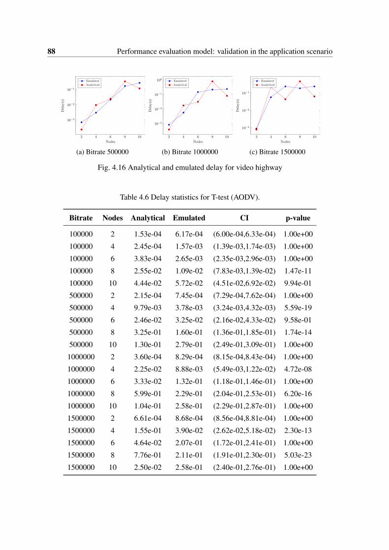
88 Performance evaluation model: validation in the application scenario
2 4 6 8 10
10−3
10−2
10−1
Nodes
Delay(s)
Emulated
Analytical
(a) Bitrate 500000
2 4 6 8 10
10−3
10−2
10−1
100
Nodes
Delay(s)
Emulated
Analytical
(b) Bitrate 1000000
2 4 6 8 10
10−3
10−2
10−1
Nodes
Delay(s)
Emulated
Analytical
(c) Bitrate 1500000
Fig. 4.16 Analytical and emulated delay for video highway
Table 4.6 Delay statistics for T-test (AODV).
Bitrate Nodes Analytical Emulated CI p-value
100000 2 1.53e-04 6.17e-04 (6.00e-04,6.33e-04) 1.00e+00
100000 4 2.45e-04 1.57e-03 (1.39e-03,1.74e-03) 1.00e+00
100000 6 3.83e-04 2.65e-03 (2.35e-03,2.96e-03) 1.00e+00
100000 8 2.55e-02 1.09e-02 (7.83e-03,1.39e-02) 1.47e-11
100000 10 4.44e-02 5.72e-02 (4.51e-02,6.92e-02) 9.94e-01
500000 2 2.15e-04 7.45e-04 (7.29e-04,7.62e-04) 1.00e+00
500000 4 9.79e-03 3.78e-03 (3.24e-03,4.32e-03) 5.59e-19
500000 6 2.46e-02 3.25e-02 (2.16e-02,4.33e-02) 9.58e-01
500000 8 3.25e-01 1.60e-01 (1.36e-01,1.85e-01) 1.74e-14
500000 10 1.30e-01 2.79e-01 (2.49e-01,3.09e-01) 1.00e+00
1000000 2 3.60e-04 8.29e-04 (8.15e-04,8.43e-04) 1.00e+00
1000000 4 2.25e-02 8.88e-03 (5.49e-03,1.22e-02) 4.72e-08
1000000 6 3.33e-02 1.32e-01 (1.18e-01,1.46e-01) 1.00e+00
1000000 8 5.99e-01 2.29e-01 (2.04e-01,2.53e-01) 6.20e-16
1000000 10 1.04e-01 2.58e-01 (2.29e-01,2.87e-01) 1.00e+00
1500000 2 6.61e-04 8.68e-04 (8.56e-04,8.81e-04) 1.00e+00
1500000 4 1.55e-01 3.90e-02 (2.62e-02,5.18e-02) 2.30e-13
1500000 6 4.64e-02 2.07e-01 (1.72e-01,2.41e-01) 1.00e+00
1500000 8 7.76e-01 2.11e-01 (1.91e-01,2.30e-01) 5.03e-23
1500000 10 2.50e-02 2.58e-01 (2.40e-01,2.76e-01) 1.00e+00
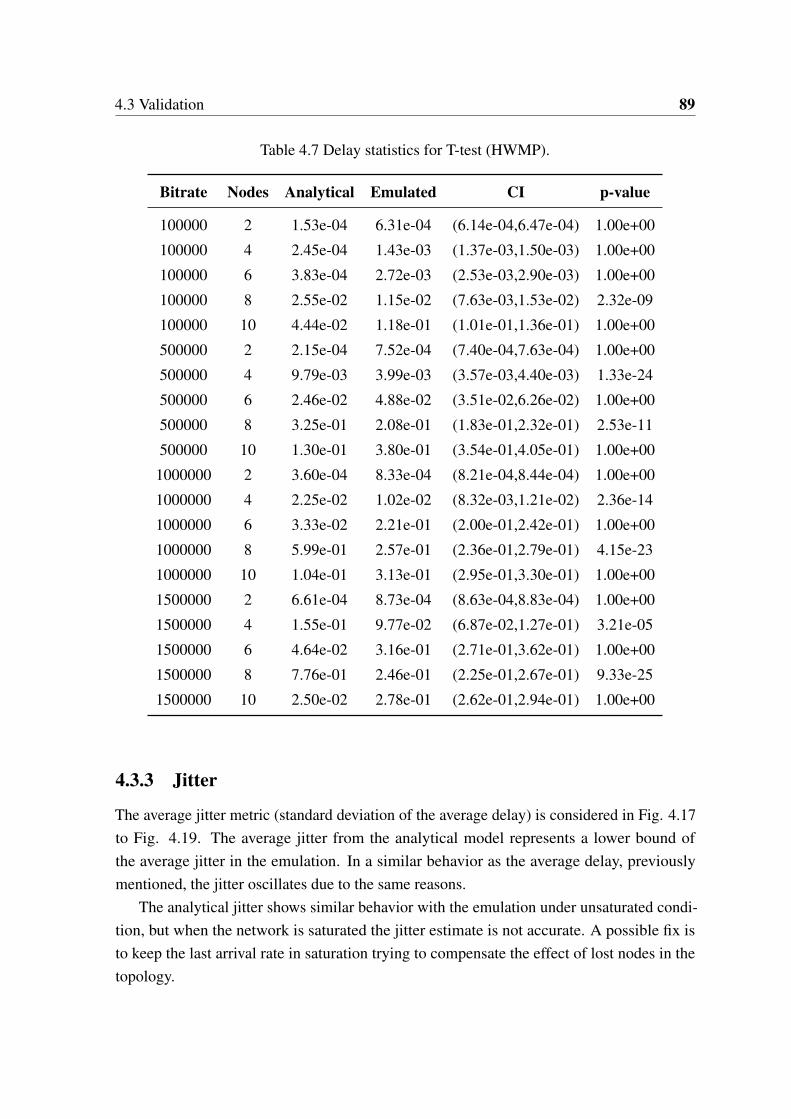
4.3 Validation 89
Table 4.7 Delay statistics for T-test (HWMP).
Bitrate Nodes Analytical Emulated CI p-value
100000 2 1.53e-04 6.31e-04 (6.14e-04,6.47e-04) 1.00e+00
100000 4 2.45e-04 1.43e-03 (1.37e-03,1.50e-03) 1.00e+00
100000 6 3.83e-04 2.72e-03 (2.53e-03,2.90e-03) 1.00e+00
100000 8 2.55e-02 1.15e-02 (7.63e-03,1.53e-02) 2.32e-09
100000 10 4.44e-02 1.18e-01 (1.01e-01,1.36e-01) 1.00e+00
500000 2 2.15e-04 7.52e-04 (7.40e-04,7.63e-04) 1.00e+00
500000 4 9.79e-03 3.99e-03 (3.57e-03,4.40e-03) 1.33e-24
500000 6 2.46e-02 4.88e-02 (3.51e-02,6.26e-02) 1.00e+00
500000 8 3.25e-01 2.08e-01 (1.83e-01,2.32e-01) 2.53e-11
500000 10 1.30e-01 3.80e-01 (3.54e-01,4.05e-01) 1.00e+00
1000000 2 3.60e-04 8.33e-04 (8.21e-04,8.44e-04) 1.00e+00
1000000 4 2.25e-02 1.02e-02 (8.32e-03,1.21e-02) 2.36e-14
1000000 6 3.33e-02 2.21e-01 (2.00e-01,2.42e-01) 1.00e+00
1000000 8 5.99e-01 2.57e-01 (2.36e-01,2.79e-01) 4.15e-23
1000000 10 1.04e-01 3.13e-01 (2.95e-01,3.30e-01) 1.00e+00
1500000 2 6.61e-04 8.73e-04 (8.63e-04,8.83e-04) 1.00e+00
1500000 4 1.55e-01 9.77e-02 (6.87e-02,1.27e-01) 3.21e-05
1500000 6 4.64e-02 3.16e-01 (2.71e-01,3.62e-01) 1.00e+00
1500000 8 7.76e-01 2.46e-01 (2.25e-01,2.67e-01) 9.33e-25
1500000 10 2.50e-02 2.78e-01 (2.62e-01,2.94e-01) 1.00e+00
4.3.3 Jitter
The average jitter metric (standard deviation of the average delay) is considered in Fig. 4.17to Fig. 4.19. The average jitter from the analytical model represents a lower bound ofthe average jitter in the emulation. In a similar behavior as the average delay, previouslymentioned, the jitter oscillates due to the same reasons.
The analytical jitter shows similar behavior with the emulation under unsaturated condi-tion, but when the network is saturated the jitter estimate is not accurate. A possible fix isto keep the last arrival rate in saturation trying to compensate the effect of lost nodes in thetopology.
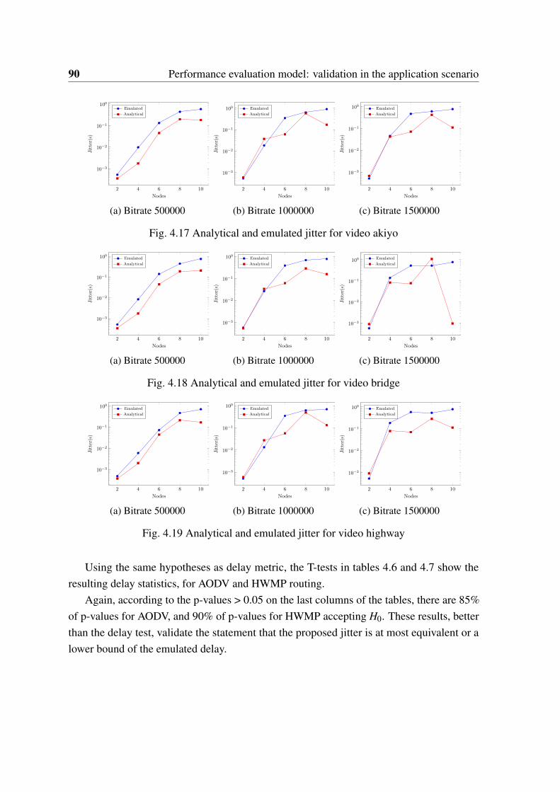
90 Performance evaluation model: validation in the application scenario
2 4 6 8 10
10−3
10−2
10−1
100
Nodes
Jitter(s)
Emulated
Analytical
(a) Bitrate 500000
2 4 6 8 10
10−3
10−2
10−1
100
Nodes
Jitter(s)
Emulated
Analytical
(b) Bitrate 1000000
2 4 6 8 10
10−3
10−2
10−1
100
Nodes
Jitter(s)
Emulated
Analytical
(c) Bitrate 1500000
Fig. 4.17 Analytical and emulated jitter for video akiyo
2 4 6 8 10
10−3
10−2
10−1
100
Nodes
Jitter(s)
Emulated
Analytical
(a) Bitrate 500000
2 4 6 8 10
10−3
10−2
10−1
100
Nodes
Jitter(s)
Emulated
Analytical
(b) Bitrate 1000000
2 4 6 8 10
10−3
10−2
10−1
100
NodesJitter(s)
Emulated
Analytical
(c) Bitrate 1500000
Fig. 4.18 Analytical and emulated jitter for video bridge
2 4 6 8 10
10−3
10−2
10−1
100
Nodes
Jitter(s)
Emulated
Analytical
(a) Bitrate 500000
2 4 6 8 10
10−3
10−2
10−1
100
Nodes
Jitter(s)
Emulated
Analytical
(b) Bitrate 1000000
2 4 6 8 10
10−3
10−2
10−1
100
Nodes
Jitter(s)
Emulated
Analytical
(c) Bitrate 1500000
Fig. 4.19 Analytical and emulated jitter for video highway
Using the same hypotheses as delay metric, the T-tests in tables 4.6 and 4.7 show theresulting delay statistics, for AODV and HWMP routing.
Again, according to the p-values > 0.05 on the last columns of the tables, there are 85%of p-values for AODV, and 90% of p-values for HWMP accepting H0. These results, betterthan the delay test, validate the statement that the proposed jitter is at most equivalent or alower bound of the emulated delay.
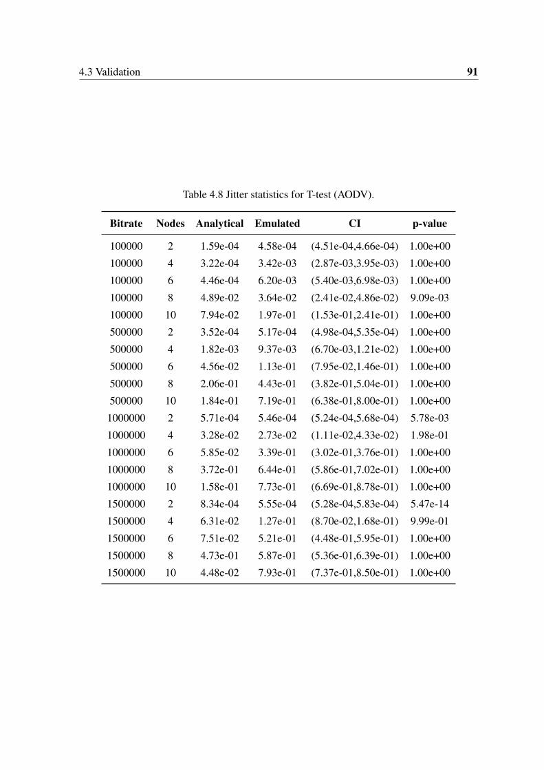
4.3 Validation 91
Table 4.8 Jitter statistics for T-test (AODV).
Bitrate Nodes Analytical Emulated CI p-value
100000 2 1.59e-04 4.58e-04 (4.51e-04,4.66e-04) 1.00e+00
100000 4 3.22e-04 3.42e-03 (2.87e-03,3.95e-03) 1.00e+00
100000 6 4.46e-04 6.20e-03 (5.40e-03,6.98e-03) 1.00e+00
100000 8 4.89e-02 3.64e-02 (2.41e-02,4.86e-02) 9.09e-03
100000 10 7.94e-02 1.97e-01 (1.53e-01,2.41e-01) 1.00e+00
500000 2 3.52e-04 5.17e-04 (4.98e-04,5.35e-04) 1.00e+00
500000 4 1.82e-03 9.37e-03 (6.70e-03,1.21e-02) 1.00e+00
500000 6 4.56e-02 1.13e-01 (7.95e-02,1.46e-01) 1.00e+00
500000 8 2.06e-01 4.43e-01 (3.82e-01,5.04e-01) 1.00e+00
500000 10 1.84e-01 7.19e-01 (6.38e-01,8.00e-01) 1.00e+00
1000000 2 5.71e-04 5.46e-04 (5.24e-04,5.68e-04) 5.78e-03
1000000 4 3.28e-02 2.73e-02 (1.11e-02,4.33e-02) 1.98e-01
1000000 6 5.85e-02 3.39e-01 (3.02e-01,3.76e-01) 1.00e+00
1000000 8 3.72e-01 6.44e-01 (5.86e-01,7.02e-01) 1.00e+00
1000000 10 1.58e-01 7.73e-01 (6.69e-01,8.78e-01) 1.00e+00
1500000 2 8.34e-04 5.55e-04 (5.28e-04,5.83e-04) 5.47e-14
1500000 4 6.31e-02 1.27e-01 (8.70e-02,1.68e-01) 9.99e-01
1500000 6 7.51e-02 5.21e-01 (4.48e-01,5.95e-01) 1.00e+00
1500000 8 4.73e-01 5.87e-01 (5.36e-01,6.39e-01) 1.00e+00
1500000 10 4.48e-02 7.93e-01 (7.37e-01,8.50e-01) 1.00e+00
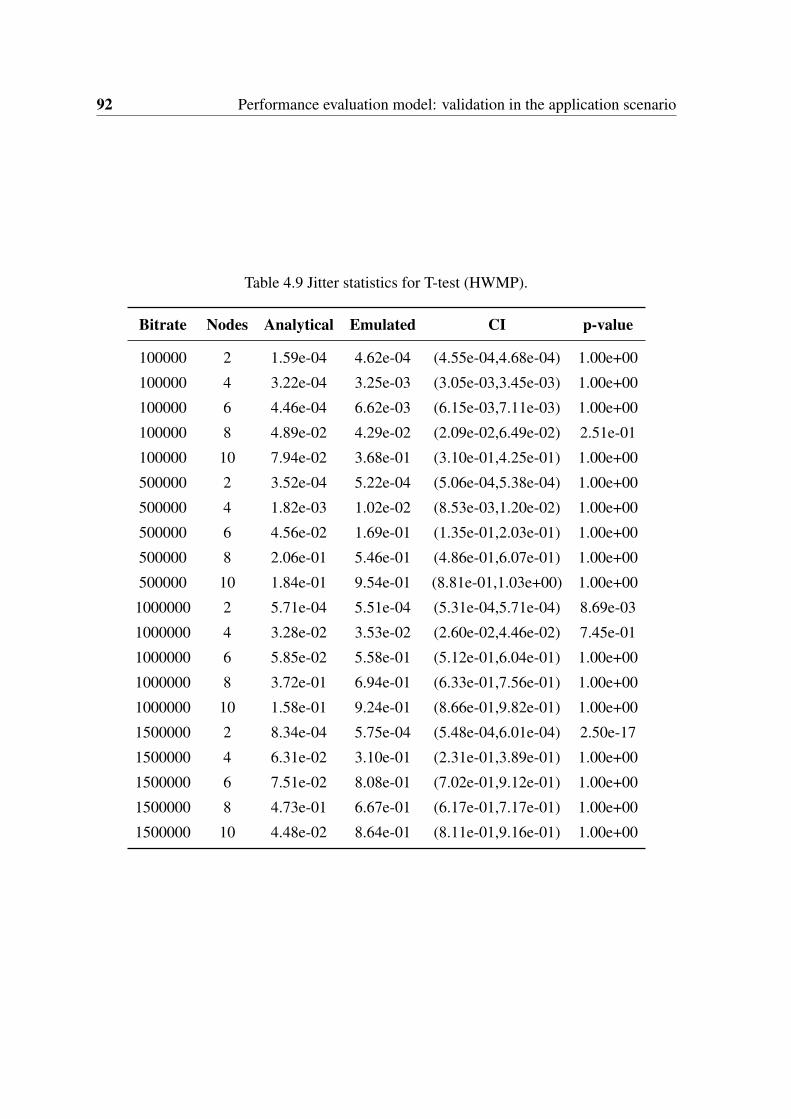
92 Performance evaluation model: validation in the application scenario
Table 4.9 Jitter statistics for T-test (HWMP).
Bitrate Nodes Analytical Emulated CI p-value
100000 2 1.59e-04 4.62e-04 (4.55e-04,4.68e-04) 1.00e+00
100000 4 3.22e-04 3.25e-03 (3.05e-03,3.45e-03) 1.00e+00
100000 6 4.46e-04 6.62e-03 (6.15e-03,7.11e-03) 1.00e+00
100000 8 4.89e-02 4.29e-02 (2.09e-02,6.49e-02) 2.51e-01
100000 10 7.94e-02 3.68e-01 (3.10e-01,4.25e-01) 1.00e+00
500000 2 3.52e-04 5.22e-04 (5.06e-04,5.38e-04) 1.00e+00
500000 4 1.82e-03 1.02e-02 (8.53e-03,1.20e-02) 1.00e+00
500000 6 4.56e-02 1.69e-01 (1.35e-01,2.03e-01) 1.00e+00
500000 8 2.06e-01 5.46e-01 (4.86e-01,6.07e-01) 1.00e+00
500000 10 1.84e-01 9.54e-01 (8.81e-01,1.03e+00) 1.00e+00
1000000 2 5.71e-04 5.51e-04 (5.31e-04,5.71e-04) 8.69e-03
1000000 4 3.28e-02 3.53e-02 (2.60e-02,4.46e-02) 7.45e-01
1000000 6 5.85e-02 5.58e-01 (5.12e-01,6.04e-01) 1.00e+00
1000000 8 3.72e-01 6.94e-01 (6.33e-01,7.56e-01) 1.00e+00
1000000 10 1.58e-01 9.24e-01 (8.66e-01,9.82e-01) 1.00e+00
1500000 2 8.34e-04 5.75e-04 (5.48e-04,6.01e-04) 2.50e-17
1500000 4 6.31e-02 3.10e-01 (2.31e-01,3.89e-01) 1.00e+00
1500000 6 7.51e-02 8.08e-01 (7.02e-01,9.12e-01) 1.00e+00
1500000 8 4.73e-01 6.67e-01 (6.17e-01,7.17e-01) 1.00e+00
1500000 10 4.48e-02 8.64e-01 (8.11e-01,9.16e-01) 1.00e+00
4.4 Conclusions 93
4.4 Conclusions
In this chapter, the proposed MHWN performance model is validated against a real P2P-TVstreaming application running on a MHWN emulated in NS-3. The NS-3 emulation model isa closer approximation to a real application scenario, using Linux containers to include realtraffic to a simulated environment.
The collaborative feature in the multihop transmission process, from the application layerand the MAC layer, validates the statistical analysis in the Poisson assumption. Here, theassumption is that in steady state, the P2P-TV application running on each node receive andforward packets, so every node in the network share traffic at a similar rate. If the number ofpackets is high during the video streaming, and the network is not in saturation state, thenthe Poisson process is a valid approximation. The validation of the Poisson process, is doneusing the histogram inter-arrival times to the queues, showing a linear trend in logarithmicscale, similar to the exponential distribution. Also, the coefficients of variation are close to1, for the same exponential distribution. A Poisson process is not self-similar with Hurstparameter equal to 0.5. Then, under normal operations of the network and the application,the traces shows a Hurst value close to 0.5. When the traffic is light the Hurst parameter isless than 0.5, and when the network is saturated the Hurst parameter is greater than 0.5.
The global performance of the MHWN is highly dependent on the P2P-TV topologyand streaming control, and on the available wireless resources. From the application layerperspective, most of the streaming applications work properly over wired networks, butin wireless environment several adjustments have to be done. As it was showed, whenincreasing the number of nodes beyond the application capacity, the throughput degrades dueto collisions, generating loss and delay in video and control packets. This suggests that theP2P-TV applications, and other streaming video applications, should integrate informationfrom lower layers, in order to fit better quality levels. Although, the P2P-TV streamingapplication is able to inject several copies of the video stream, increasing the number suchcopies generates a large drift between emulation time and real time, affecting the globalresults of the testbed.
From the MAC layer perspective the proposed analytical MHWN model is a reliableapproach to evaluate the performance of the network. The analytical throughput estimate is agood approximation considering an upper bound limit. The T-test confirms the approximation,as in the case of AODV is 90%, and 95% for HWMP, using the number of p-values > 0.05accepting the hypothesis. The estimated delay is a lower bound in 65% of p-values forAODV, and 65% of p-values for HWMP. In the case of jitter, there is a better approximationof the estimated values as a lower bound of the simulated value, with 85% of p-values forAODV, and 90% of p-values for HWMP, accepting the lower bound hypothesis. These

94 Performance evaluation model: validation in the application scenario
results, despite the oscillations in the delay and jitter values, validates the statement that theestimated delay and jitter metrics are at most equivalent or a lower bound of the emulatedequivalent metrics. Them, the performance MHWN evaluation model presents satisfactoryresults estimating the QoS metrics compared with the emulation model.
Such results are promising considering the complexity associated in the transmissionprocess developed by the P2P-TV application integrated with the NS-3 in real-time emulationmode. Further research is required to obtain closer estimates with emulation, and with theappropriate extensions to the model, it could improve the expected results.
Chapter 5
Statistical performance evaluation ofP2P video streaming on MHWN
5.1 Introduction
P2P streaming services can be deployed in a IEEE 802.11 MHWN, in a typical applicationscenario like e-learning, in a wireless campus network. Such MHWN present problemsproviding the expected quality levels required by the streaming applications. The proposedperformance model estimates the expected QoS metrics, with a good level of accuracy.However, the proposed MHWN performance model has its limitations, taking into accountthe simplifications and the reduced number of factors included in the model. These approxi-mations are required to set an adequate level of complexity, and trying to keep the modelanalytically tractable. In order to enhance the model, other factors can be included in themodel, but there are many possible factors at each layer, and sometimes they can not bemodeled, due to excessive complexity. Hence, a statistical analysis is required in order todetermine other factors that influence the quality of the P2P video streaming on MHWN.
Different quality metrics are used to evaluate the video streaming performance. Tradi-tionally, the QoS metrics evaluate the performance from the MAC layer perspective, andquality of experience (QoE) metrics from the application layer perspective. Considering this,a global quality score can be established relating the quality metrics at different layers. Thisscore defines several operation ranges in terms of QoS and QoE metrics.
In this chapter, we use multivariate statistical analysis in order to reveal the factorsthat influence the quality of P2P streaming on a MHWN. Initially, a literature review ispresented showing similar approaches. Then, the statistical framework is described using themulti-variate regression analysis, and the application of K-means clustering process in the
96 Statistical performance evaluation of P2P video streaming on MHWN
relationship between QoS and QoE metrics. The experimental unit is based on a MHWNdeveloped in NS-3, the same as in the previous chapter.
5.2 Streaming video quality evaluation
User satisfaction is a main concern in streaming video applications. The network operatorscontinuously monitor and control their wireless resources in order to maintain appropriatequality levels. From a global perspective, an appropriate quality evaluation should considerboth QoS and QoE metrics [149].
5.2.1 Quality from the application layer perspective
Performance video quality metrics are evaluated through objective and subjective measures.Objective metrics rely on different statistics obtained by comparing the original and thedistorted video. One of such metrics is the Peak Signal to Noise Ratio (PSNR), which is theratio between the maximum power of the original video and the power of the interfering noiseintroduced in the transmission process. The Structural Similarity Index (SSIM) is designedto improve traditional methods like PSNR, using a statistic relating different moments inthe spatial similarity. The Video Quality Metric (VQM) method objectively measures videoquality by comparing the original and the distorted video sequences using only a set offeatures extracted from each video [150][151].
Subjective video evaluation is developed by individuals, scoring in a determinate scalethe video quality based on a reference. In this context, QoE is the overall acceptability of anapplication or service, as perceived by end-users [152][150]. A typical representation of QoEis the Mean Opinion Score (MOS), which measures the distortion from the user perspectiveon a pre-defined scale [153][149]. According to [153] there is a possible relation betweenPSNR and MOS. Subjective video quality estimations are standardized by ITU-R BT.500-11specifying several variants (Single Stimulus SS, Double Stimulus Impairment Scale (DSIS),Double Stimulus Continuous Quality Scale (DSCQS), etc.). Among all these variants, theSS (Single Stimulus) is a better approach in quality assessment with simplicity [154].
Streaming applications require QoE assessment in real-time, and the methods mentioneduse off-line evaluation based on full reference or reduced reference videos (subjective orobjective). Besides objective methods are not well correlated with human visual perceptionand they are time consuming [155]. In most of streaming video implementations it is notpossible to access the reference videos, and the quality evaluation must be done without any
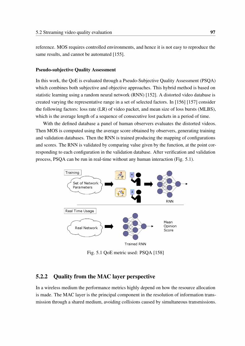
5.2 Streaming video quality evaluation 97
reference. MOS requires controlled environments, and hence it is not easy to reproduce thesame results, and cannot be automated [155].
Pseudo-subjective Quality Assessment
In this work, the QoE is evaluated through a Pseudo-Subjective Quality Assessment (PSQA)which combines both subjective and objective approaches. This hybrid method is based onstatistic learning using a random neural network (RNN) [152]. A distorted video database iscreated varying the representative range in a set of selected factors. In [156] [157] considerthe following factors: loss rate (LR) of video packet, and mean size of loss bursts (MLBS),which is the average length of a sequence of consecutive lost packets in a period of time.
With the defined database a panel of human observers evaluates the distorted videos.Then MOS is computed using the average score obtained by observers, generating trainingand validation databases. Then the RNN is trained producing the mapping of configurationsand scores. The RNN is validated by comparing value given by the function, at the point cor-responding to each configuration in the validation database. After verification and validationprocess, PSQA can be run in real-time without any human interaction (Fig. 5.1).
Fig. 5.1 QoE metric used: PSQA [158]
5.2.2 Quality from the MAC layer perspective
In a wireless medium the performance metrics highly depend on how the resource allocationis made. The MAC layer is the principal component in the resolution of information trans-mission through a shared medium, avoiding collisions caused by simultaneous transmissions.
98 Statistical performance evaluation of P2P video streaming on MHWN
Most of the performance models are focused on the estimation of QoS metrics like through-put, delay and jitter [91]. The IEEE 802.11 MAC layer uses a contention access schemedesigned to reduce collisions due to the simultaneous transmission of multiple sources ona shared channel. This scheme is implemented using a Distributed Coordination Function(DCF) based on the Carrier Sense Medium Access with Collision Avoidance (CSMA/CA)protocol [91]. These schemes create fairness problems considering the access to the mediumis given on a first-come first-served basis. The MAC layer with QoS enhancements aims atproviding reduced overhead, priority access, and reduced number of collisions [159].
5.3 Related work
Finding a relationship between QoS and QoE is a challenging task in streaming video. Suchrelationship is a significant feedback mechanism in order to provide reliable multimediaservices.
Alreshoodi and Woods [160] presents a survey of QoS/QoE correlation approaches. Theauthors conclude that there is a need to identify and understand many QoE influencing factorsfor a given type of service and how they relate to each other.
Mok et al. [161] focuses on how the network QoS affects the QoE of HTTP videostreaming. They found the correlation between the network QoS and application QoS, andmeasured the correlation between application QoS and QoE. Du et al. [162] used a neuralnetwork to establish a relationship between the network parameters and a QoE metric.
An Analysis of Variance (ANOVA) is used in [163], where the authors found the appro-priate set of parameters based on performance QoS metrics, in terms of energy consumption.The experimental design was a wireless body area network implemented in OMNeT++, andin a real hardware platform. In [164] the authors use multivariate ANOVA to characterize theinteraction between the input variables of a wireless network simulation (NS-2). The contextis the cross-layer interaction between MANET protocols, network topology, and propagationconditions.
Recently in [165], Bustos-Jimenez et al. introduced a modular framework, based onNS-3 and Linux Containers (LXC), to study the relation between QoS and QoE metrics formultimedia transmissions, including framerate and jitter metrics in the VLC media player(VideoLan).
5.4 Statistical performance evaluation 99
5.4 Statistical performance evaluation
The quality of P2P streaming video is generally evaluated using objective or subjectivemetrics. But this task is even more complex in wireless multihop environments. This sectiondescribes the statistical framework developed to evaluate the quality of P2P video streamingon an MHWN. First, we determine the factors that influence the performance of the P2Pvideo streaming, using a multi-variate regression analysis. Then, we establish a relationshipbetween QoS and QoE metrics of the P2P video streaming using clustering analysis.
5.4.1 Multi-variate regression analysis
Let yi , i = 1,2, . . . ,n represent the observed values from a dependent or response variableY . Let xi j, denote the corresponding values for the independent or explanatory variablesX1,X2, . . . ,Xp. A multiple linear regression model is defined as:
yi = β0 +β1xi1 +β2xi2 + · · ·+βpxip + εi (5.1)
where β j denote the unknown regression parameters, and εi ∼ N(0,σ2) is the error ofeach observed response.
Many factors may affect the P2P streaming performance on MHWN, depending on thewireless channel, the topology, the routing protocol, the OSI layer protocols, and the videocoding. A reduced number of factors has been selected, only considering relevant factorsthat may affect the video quality, thus reducing the number of experiments. The influenceof these factors on the streaming video quality is analyzed through the defined multivariateregression model. The factors are the independent variables, and the quality metrics are thedependent variables in the regression model.
The selected factors are the number of stations, the video bitrate transmission, an MHWNon a regular grid topology with four-neighbor and eight-neighbor connections depending onthe distance of the nodes, reactive routing (AODV: Ad hoc On-Demand Distance Vector)and a hybrid approach using proactive-reactive routing (Hybrid Wireless Mesh Protocol),and five reference videos with the same encoding process and no audio (See Table 5.1). Theoutput or response variables are the following QoS metrics: throughput, delay and jitter, andthe real-time QoE metric from the P2P video streaming application. The regression model isuseful to estimate the QoS metrics based in Eq.5.1, considering the defined input parametersin table 5.1.
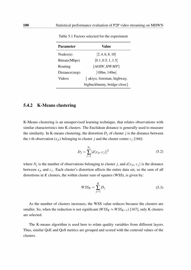
100 Statistical performance evaluation of P2P video streaming on MHWN
Table 5.1 Factors selected for the experiment
Parameter Value
Nodes(n) [2,4,6,8,10]
Bitrate(Mbps) [0.1,0.5,1,1.5]
Routing AODV,HWMPDistance(step) [100m,140m]
Videos akiyo, foreman, highway,
bigbuckbunny, bridge-close
5.4.2 K-Means clustering
K-Means clustering is an unsupervised learning technique, that relates observations withsimilar characteristics into K clusters. The Euclidean distance is generally used to measurethe similarity. In K-means clustering, the distortion D j of cluster j is the distance betweenthe t-th observation (x jt) belonging to cluster j and the cluster center c j [166]:
D j =N j
∑t=1
[d(x jt ,c j)]2 (5.2)
where N j is the number of observations belonging to cluster j, and d(x jt , c j) is the distancebetween x jt and c j. Each cluster’s distortion affects the entire data set, so the sum of alldistortions in K clusters, the within cluster sum of squares (WSS), is given by:
WSSK =K
∑j=1
D j (5.3)
As the number of clusters increases, the WSS value reduces because the clusters aresmaller. So, when the reduction is not significant (WSSK ≈WSSK+1) [167], only K clustersare selected.
The K-means algorithm is used here to relate quality variables from different layers.Thus, similar QoE and QoS metrics are grouped and scored with the centroid values of theclusters.
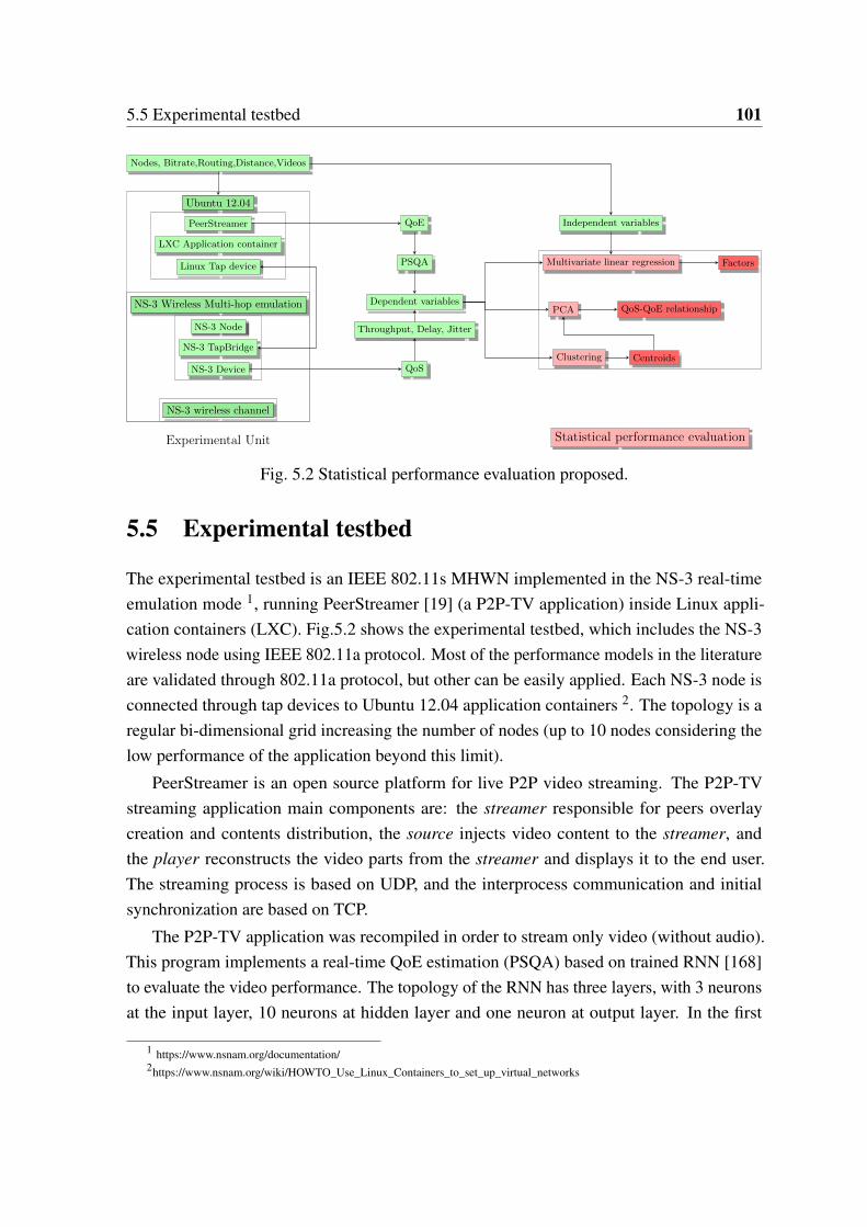
5.5 Experimental testbed 101
Ubuntu 12.04
PeerStreamer QoE
PSQA
Nodes, Bitrate,Routing,Distance,Videos
Dependent variables
Independent variables
Multivariate linear regression
Clustering
PCA
Centroids
Factors
QoS-QoE relationship
Statistical performance evaluation
LXC Application container
Linux Tap device
NS-3 Wireless Multi-hop emulation
NS-3 Node
NS-3 TapBridge
NS-3 Device QoS
Throughput, Delay, Jitter
NS-3 wireless channel
Experimental Unit
Fig. 5.2 Statistical performance evaluation proposed.
5.5 Experimental testbed
The experimental testbed is an IEEE 802.11s MHWN implemented in the NS-3 real-timeemulation mode 1, running PeerStreamer [19] (a P2P-TV application) inside Linux appli-cation containers (LXC). Fig.5.2 shows the experimental testbed, which includes the NS-3wireless node using IEEE 802.11a protocol. Most of the performance models in the literatureare validated through 802.11a protocol, but other can be easily applied. Each NS-3 node isconnected through tap devices to Ubuntu 12.04 application containers 2. The topology is aregular bi-dimensional grid increasing the number of nodes (up to 10 nodes considering thelow performance of the application beyond this limit).
PeerStreamer is an open source platform for live P2P video streaming. The P2P-TVstreaming application main components are: the streamer responsible for peers overlaycreation and contents distribution, the source injects video content to the streamer, andthe player reconstructs the video parts from the streamer and displays it to the end user.The streaming process is based on UDP, and the interprocess communication and initialsynchronization are based on TCP.
The P2P-TV application was recompiled in order to stream only video (without audio).This program implements a real-time QoE estimation (PSQA) based on trained RNN [168]to evaluate the video performance. The topology of the RNN has three layers, with 3 neuronsat the input layer, 10 neurons at hidden layer and one neuron at output layer. In the first
1 https://www.nsnam.org/documentation/2https://www.nsnam.org/wiki/HOWTO_Use_Linux_Containers_to_set_up_virtual_networks
102 Statistical performance evaluation of P2P video streaming on MHWN
layer the inputs are LR, MLBS and Bit-rate. The normalized output is scaled to obtain areal-time QoE value, updated every 0.5 seconds. The application generates QoE traces (inPSNR scale), and I-B-P received sequences. The authors in [146] used PeerStreamer forquality video assessment over a wireless mesh network.
The input video is looped, and then it is streamed to n−1 nodes using one server nodeduring 5 minutes, for each replication, with one minute of network setup time.
The QoS metrics are extracted from the generated traces at the end of the emulationprocess, using AWK scripts.
T hroughput =Total received payload
time last rx− time first tx
Delay =total delay
total received packets
Jitter =
√total delay2
total received packets−Delay2
(5.4)
5.6 Results
In order to obtain significant results, 400 experiments where conducted. Each video istransmitted during five minutes, with three independent runs per trial. The traces extractedfrom each experiment form the independent and dependent variables set in the multivariateregression process. The multivariate regression process is developed in the statistical softwareR with the command lm [169], which returns model coefficients (βi) and regression statistics,as shown in Table 5.2.
The dummy variable in all regressions is the video "akiyo". The resulting coefficientsof the regression influence the quality metrics, if the t-test value accepts the alternativehypothesis that the coefficients are different from zero, with a p-value < 10−3 (confidence of99.999%).
The influencing factors in throughput are highlighted in Table 5.2. In this regressionmodel all selected factors were included plus one interaction between the number of nodesand the bitrate. From the p-value results, the routing and the type of video do not affectthe performance, using the same encoding process and a constant bitrate. The F test alsovalidates the appropriate fit in each model. The throughput can be modeled using only therelevant factors according to p-value, as shown in Table 5.3.
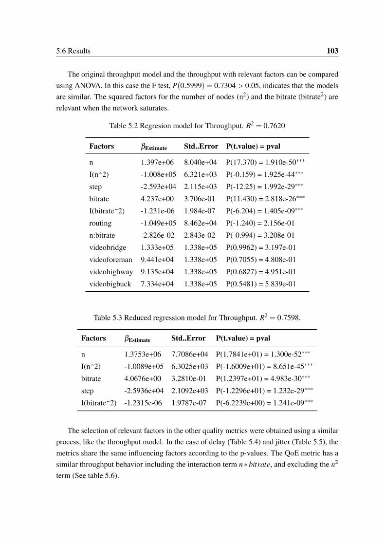
5.6 Results 103
The original throughput model and the throughput with relevant factors can be comparedusing ANOVA. In this case the F test, P(0.5999) = 0.7304 > 0.05, indicates that the modelsare similar. The squared factors for the number of nodes (n2) and the bitrate (bitrate2) arerelevant when the network saturates.
Table 5.2 Regresion model for Throughput. R2 = 0.7620
Factors βEstimate Std..Error P(t.value) = pval
n 1.397e+06 8.040e+04 P(17.370) = 1.910e-50∗∗∗
I(n^2) -1.008e+05 6.321e+03 P(-0.159) = 1.925e-44∗∗∗
step -2.593e+04 2.115e+03 P(-12.25) = 1.992e-29∗∗∗
bitrate 4.237e+00 3.706e-01 P(11.430) = 2.818e-26∗∗∗
I(bitrate^2) -1.231e-06 1.984e-07 P(-6.204) = 1.405e-09∗∗∗
routing -1.049e+05 8.462e+04 P(-1.240) = 2.156e-01
n:bitrate -2.826e-02 2.843e-02 P(-0.994) = 3.208e-01
videobridge 1.333e+05 1.338e+05 P(0.9962) = 3.197e-01
videoforeman 9.441e+04 1.338e+05 P(0.7055) = 4.808e-01
videohighway 9.135e+04 1.338e+05 P(0.6827) = 4.951e-01
videobigbuck 7.334e+04 1.338e+05 P(0.5481) = 5.839e-01
Table 5.3 Reduced regression model for Throughput. R2 = 0.7598.
Factors βEstimate Std..Error P(t.value) = pval
n 1.3753e+06 7.7086e+04 P(1.7841e+01) = 1.300e-52∗∗∗
I(n^2) -1.0089e+05 6.3025e+03 P(-1.6009e+01) = 8.651e-45∗∗∗
bitrate 4.0676e+00 3.2810e-01 P(1.2397e+01) = 4.983e-30∗∗∗
step -2.5936e+04 2.1092e+03 P(-1.2296e+01) = 1.232e-29∗∗∗
I(bitrate^2) -1.2315e-06 1.9787e-07 P(-6.2239e+00) = 1.241e-09∗∗∗
The selection of relevant factors in the other quality metrics were obtained using a similarprocess, like the throughput model. In the case of delay (Table 5.4) and jitter (Table 5.5), themetrics share the same influencing factors according to the p-values. The QoE metric has asimilar throughput behavior including the interaction term n∗bitrate, and excluding the n2
term (See table 5.6).
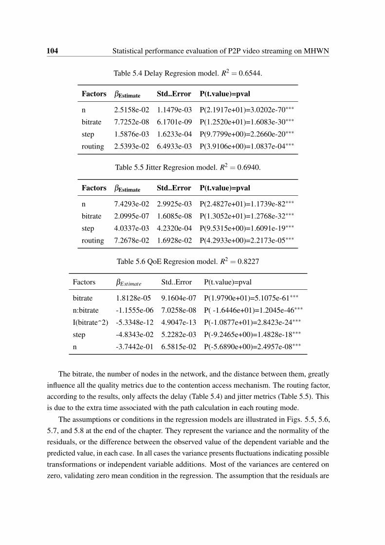
104 Statistical performance evaluation of P2P video streaming on MHWN
Table 5.4 Delay Regresion model. R2 = 0.6544.
Factors βEstimate Std..Error P(t.value)=pval
n 2.5158e-02 1.1479e-03 P(2.1917e+01)=3.0202e-70∗∗∗
bitrate 7.7252e-08 6.1701e-09 P(1.2520e+01)=1.6083e-30∗∗∗
step 1.5876e-03 1.6233e-04 P(9.7799e+00)=2.2660e-20∗∗∗
routing 2.5393e-02 6.4933e-03 P(3.9106e+00)=1.0837e-04∗∗∗
Table 5.5 Jitter Regresion model. R2 = 0.6940.
Factors βEstimate Std..Error P(t.value)=pval
n 7.4293e-02 2.9925e-03 P(2.4827e+01)=1.1739e-82∗∗∗
bitrate 2.0995e-07 1.6085e-08 P(1.3052e+01)=1.2768e-32∗∗∗
step 4.0337e-03 4.2320e-04 P(9.5315e+00)=1.6091e-19∗∗∗
routing 7.2678e-02 1.6928e-02 P(4.2933e+00)=2.2173e-05∗∗∗
Table 5.6 QoE Regresion model. R2 = 0.8227
Factors βEstimate Std..Error P(t.value)=pval
bitrate 1.8128e-05 9.1604e-07 P(1.9790e+01)=5.1075e-61∗∗∗
n:bitrate -1.1555e-06 7.0258e-08 P( -1.6446e+01)=1.2045e-46∗∗∗
I(bitrate^2) -5.3348e-12 4.9047e-13 P(-1.0877e+01)=2.8423e-24∗∗∗
step -4.8343e-02 5.2282e-03 P(-9.2465e+00)=1.4828e-18∗∗∗
n -3.7442e-01 6.5815e-02 P(-5.6890e+00)=2.4957e-08∗∗∗
The bitrate, the number of nodes in the network, and the distance between them, greatlyinfluence all the quality metrics due to the contention access mechanism. The routing factor,according to the results, only affects the delay (Table 5.4) and jitter metrics (Table 5.5). Thisis due to the extra time associated with the path calculation in each routing mode.
The assumptions or conditions in the regression models are illustrated in Figs. 5.5, 5.6,5.7, and 5.8 at the end of the chapter. They represent the variance and the normality of theresiduals, or the difference between the observed value of the dependent variable and thepredicted value, in each case. In all cases the variance presents fluctuations indicating possibletransformations or independent variable additions. Most of the variances are centered onzero, validating zero mean condition in the regression. The assumption that the residuals are
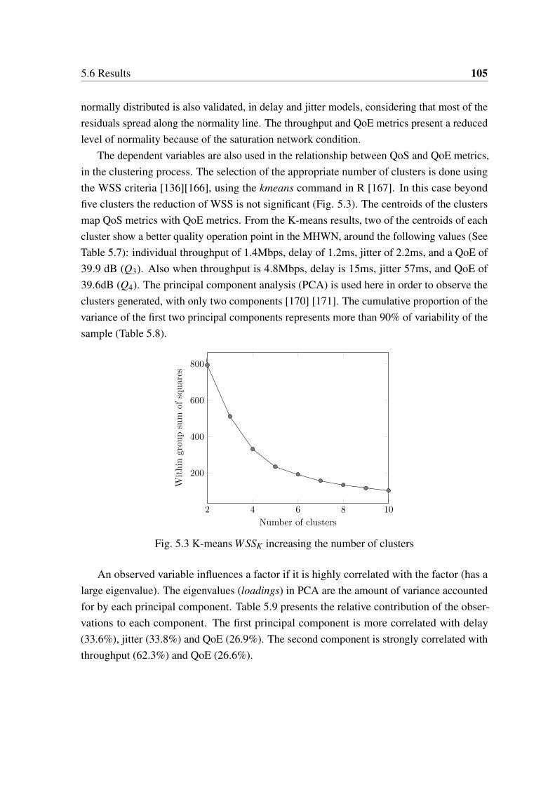
5.6 Results 105
normally distributed is also validated, in delay and jitter models, considering that most of theresiduals spread along the normality line. The throughput and QoE metrics present a reducedlevel of normality because of the saturation network condition.
The dependent variables are also used in the relationship between QoS and QoE metrics,in the clustering process. The selection of the appropriate number of clusters is done usingthe WSS criteria [136][166], using the kmeans command in R [167]. In this case beyondfive clusters the reduction of WSS is not significant (Fig. 5.3). The centroids of the clustersmap QoS metrics with QoE metrics. From the K-means results, two of the centroids of eachcluster show a better quality operation point in the MHWN, around the following values (SeeTable 5.7): individual throughput of 1.4Mbps, delay of 1.2ms, jitter of 2.2ms, and a QoE of39.9 dB (Q3). Also when throughput is 4.8Mbps, delay is 15ms, jitter 57ms, and QoE of39.6dB (Q4). The principal component analysis (PCA) is used here in order to observe theclusters generated, with only two components [170] [171]. The cumulative proportion of thevariance of the first two principal components represents more than 90% of variability of thesample (Table 5.8).
2 4 6 8 10
200
400
600
800
Number of clusters
Within
grou
psum
ofsquares
Fig. 5.3 K-means WSSK increasing the number of clusters
An observed variable influences a factor if it is highly correlated with the factor (has alarge eigenvalue). The eigenvalues (loadings) in PCA are the amount of variance accountedfor by each principal component. Table 5.9 presents the relative contribution of the obser-vations to each component. The first principal component is more correlated with delay(33.6%), jitter (33.8%) and QoE (26.9%). The second component is strongly correlated withthroughput (62.3%) and QoE (26.6%).
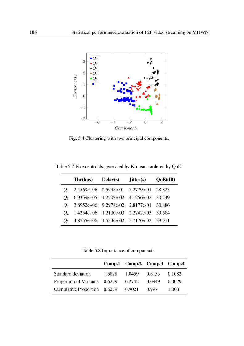
106 Statistical performance evaluation of P2P video streaming on MHWN
−6 −4 −2 0 2−2
−1
0
1
2
3
Component1
Com
pon
ent 2
Q1
Q2
Q3
Q4
Q5
Fig. 5.4 Clustering with two principal components.
Table 5.7 Five centroids generated by K-means ordered by QoE.
Thr(bps) Delay(s) Jitter(s) QoE(dB)
Q1 2.4569e+06 2.5948e-01 7.2779e-01 28.823
Q5 6.9359e+05 1.2202e-02 4.1256e-02 30.549
Q2 3.8952e+06 9.2978e-02 2.8177e-01 30.886
Q4 1.4254e+06 1.2100e-03 2.2742e-03 39.684
Q3 4.8755e+06 1.5336e-02 5.7170e-02 39.911
Table 5.8 Importance of components.
Comp.1 Comp.2 Comp.3 Comp.4
Standard deviation 1.5828 1.0459 0.6153 0.1082
Proportion of Variance 0.6279 0.2742 0.0949 0.0029
Cumulative Proportion 0.6279 0.9021 0.997 1.000
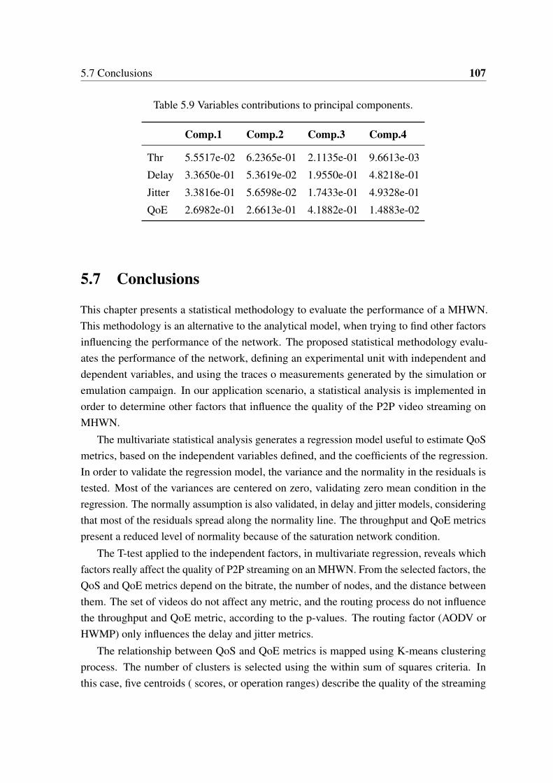
5.7 Conclusions 107
Table 5.9 Variables contributions to principal components.
Comp.1 Comp.2 Comp.3 Comp.4
Thr 5.5517e-02 6.2365e-01 2.1135e-01 9.6613e-03
Delay 3.3650e-01 5.3619e-02 1.9550e-01 4.8218e-01
Jitter 3.3816e-01 5.6598e-02 1.7433e-01 4.9328e-01
QoE 2.6982e-01 2.6613e-01 4.1882e-01 1.4883e-02
5.7 Conclusions
This chapter presents a statistical methodology to evaluate the performance of a MHWN.This methodology is an alternative to the analytical model, when trying to find other factorsinfluencing the performance of the network. The proposed statistical methodology evalu-ates the performance of the network, defining an experimental unit with independent anddependent variables, and using the traces o measurements generated by the simulation oremulation campaign. In our application scenario, a statistical analysis is implemented inorder to determine other factors that influence the quality of the P2P video streaming onMHWN.
The multivariate statistical analysis generates a regression model useful to estimate QoSmetrics, based on the independent variables defined, and the coefficients of the regression.In order to validate the regression model, the variance and the normality in the residuals istested. Most of the variances are centered on zero, validating zero mean condition in theregression. The normally assumption is also validated, in delay and jitter models, consideringthat most of the residuals spread along the normality line. The throughput and QoE metricspresent a reduced level of normality because of the saturation network condition.
The T-test applied to the independent factors, in multivariate regression, reveals whichfactors really affect the quality of P2P streaming on an MHWN. From the selected factors, theQoS and QoE metrics depend on the bitrate, the number of nodes, and the distance betweenthem. The set of videos do not affect any metric, and the routing process do not influencethe throughput and QoE metric, according to the p-values. The routing factor (AODV orHWMP) only influences the delay and jitter metrics.
The relationship between QoS and QoE metrics is mapped using K-means clusteringprocess. The number of clusters is selected using the within sum of squares criteria. Inthis case, five centroids ( scores, or operation ranges) describe the quality of the streaming
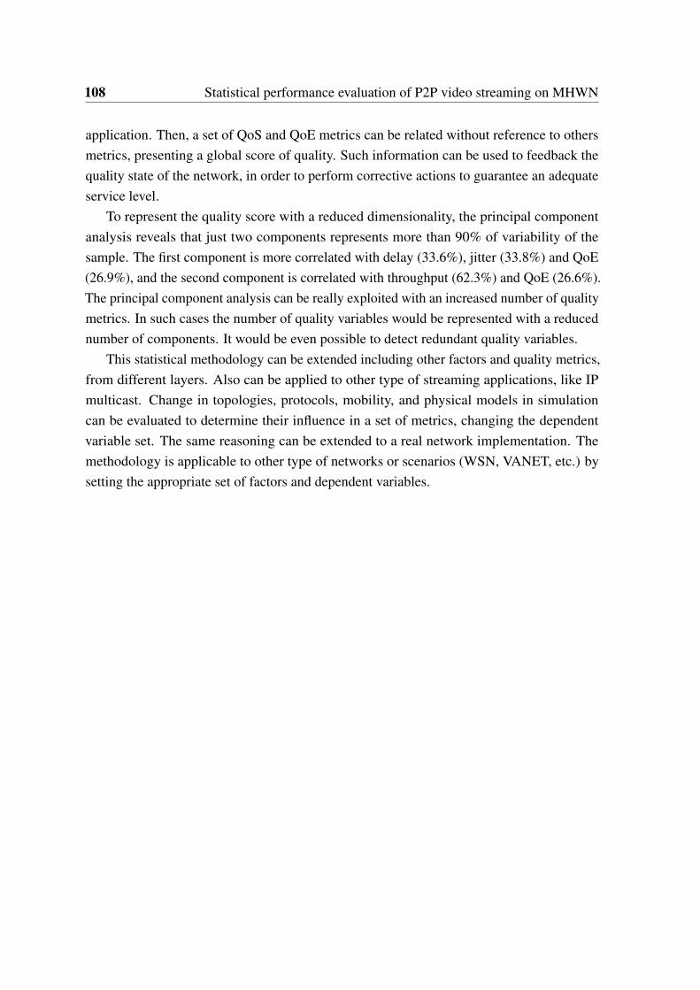
108 Statistical performance evaluation of P2P video streaming on MHWN
application. Then, a set of QoS and QoE metrics can be related without reference to othersmetrics, presenting a global score of quality. Such information can be used to feedback thequality state of the network, in order to perform corrective actions to guarantee an adequateservice level.
To represent the quality score with a reduced dimensionality, the principal componentanalysis reveals that just two components represents more than 90% of variability of thesample. The first component is more correlated with delay (33.6%), jitter (33.8%) and QoE(26.9%), and the second component is correlated with throughput (62.3%) and QoE (26.6%).The principal component analysis can be really exploited with an increased number of qualitymetrics. In such cases the number of quality variables would be represented with a reducednumber of components. It would be even possible to detect redundant quality variables.
This statistical methodology can be extended including other factors and quality metrics,from different layers. Also can be applied to other type of streaming applications, like IPmulticast. Change in topologies, protocols, mobility, and physical models in simulationcan be evaluated to determine their influence in a set of metrics, changing the dependentvariable set. The same reasoning can be extended to a real network implementation. Themethodology is applicable to other type of networks or scenarios (WSN, VANET, etc.) bysetting the appropriate set of factors and dependent variables.
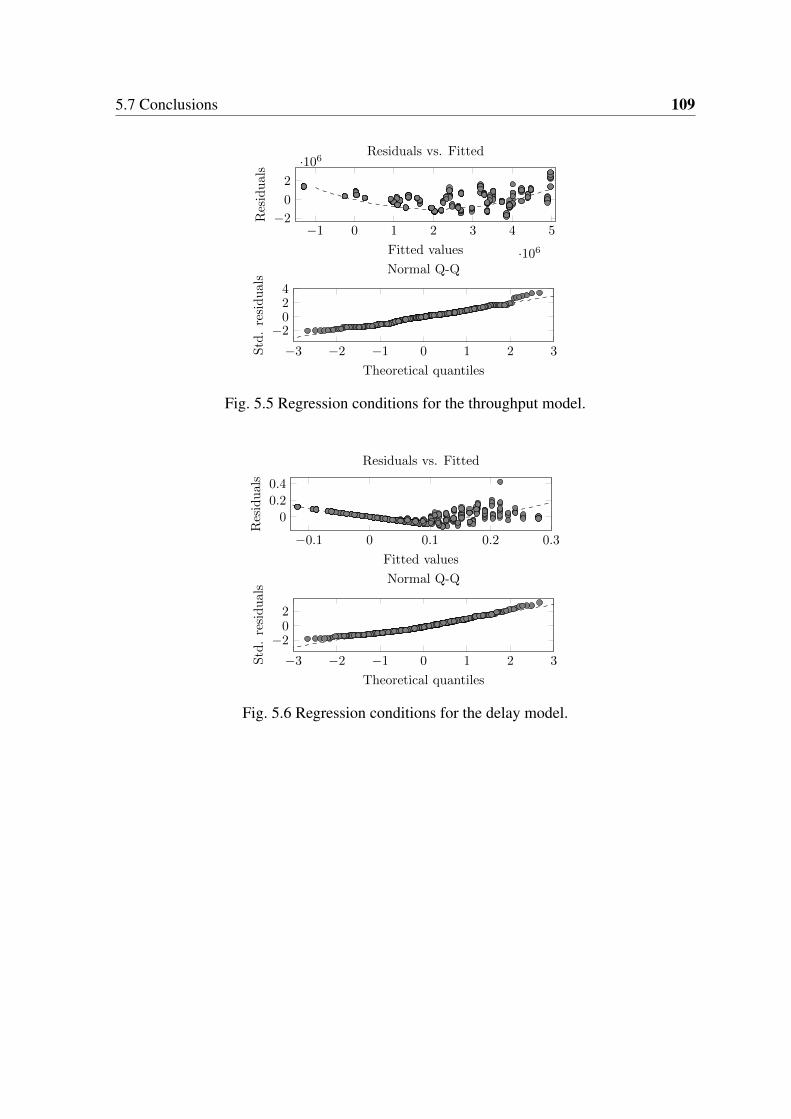
5.7 Conclusions 109
−1 0 1 2 3 4 5
·106
−20
2
·106
Fitted valuesResiduals
Residuals vs. Fitted
−3 −2 −1 0 1 2 3
−2024
Theoretical quantiles
Std.residuals
Normal Q-Q
Fig. 5.5 Regression conditions for the throughput model.
−0.1 0 0.1 0.2 0.3
0
0.2
0.4
Fitted values
Residuals
Residuals vs. Fitted
−3 −2 −1 0 1 2 3
−202
Theoretical quantiles
Std.residuals
Normal Q-Q
Fig. 5.6 Regression conditions for the delay model.
110 Statistical performance evaluation of P2P video streaming on MHWN
−0.4 −0.2 0 0.2 0.4 0.6 0.8
0
0.5
1
Fitted values
Residuals
Residuals vs. Fitted
−3 −2 −1 0 1 2 3
−202
Theoretical quantiles
Std.residuals
Normal Q-Q
Fig. 5.7 Regression conditions for the jitter model.
25 30 35 40 45−50
5
Fitted values
Residuals
Residuals vs. Fitted
−3 −2 −1 0 1 2 3
−202
Theoretical quantiles
Std.residuals
Normal Q-Q
Fig. 5.8 Regression conditions for the QoE model.
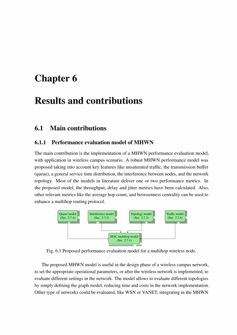
Chapter 6
Results and contributions
6.1 Main contributions
6.1.1 Performance evaluation model of MHWN
The main contribution is the implementation of a MHWN performance evaluation model,with application in wireless campus scenario. A robust MHWN performance model wasproposed taking into account key features like unsaturated traffic, the transmission buffer(queue), a general service time distribution, the interference between nodes, and the networktopology. Most of the models in literature deliver one or two performance metrics. Inthe proposed model, the throughput, delay and jitter metrics have been calculated. Also,other relevant metrics like the average hop count, and betweenness centrality can be used toenhance a multihop routing protocol.
Queue model(Sec. 2.7.4)
Interference model(Sec. 2.7.2)
Topology model(Sec. 2.7.3)
Traffic model(Sec. 2.7.4)
MAC multihop model(Sec. 2.7.1)
Fig. 6.1 Proposed performance evaluation model for a multihop wireless node.
The proposed MHWN model is useful in the design phase of a wireless campus network,to set the appropriate operational parameters, or after the wireless network is implemented, toevaluate different settings in the network. The model allows to evaluate different topologiesby simply defining the graph model, reducing time and costs in the network implementation.Other type of networks could be evaluated, like WSN or VANET, integrating in the MHWN
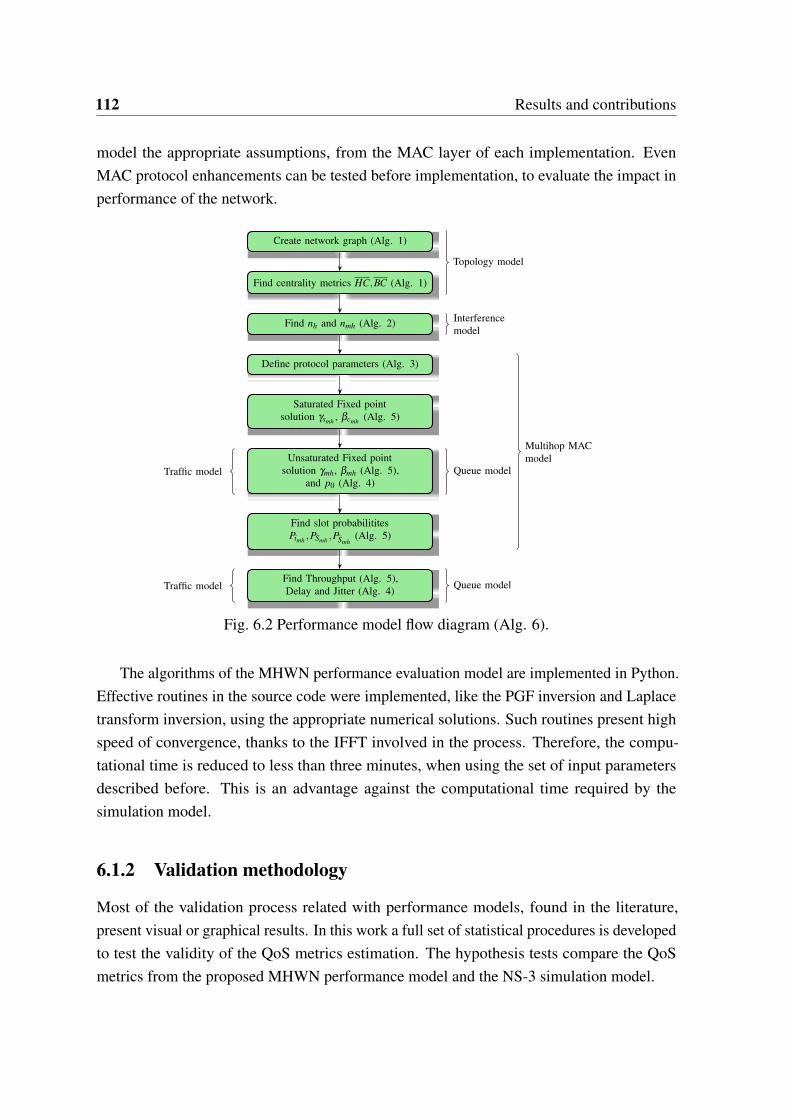
112 Results and contributions
model the appropriate assumptions, from the MAC layer of each implementation. EvenMAC protocol enhancements can be tested before implementation, to evaluate the impact inperformance of the network.
Create network graph (Alg. 1)
Find centrality metrics HC,BC (Alg. 1)
Find nh and nmh (Alg. 2)
Define protocol parameters (Alg. 3)
Saturated Fixed pointsolution γsmh , βcmh (Alg. 5)
Unsaturated Fixed pointsolution γmh, βmh (Alg. 5),
and p0 (Alg. 4)
Find slot probabilititesPimh ,PSmh ,PSmh
(Alg. 5)
Find Throughput (Alg. 5),Delay and Jitter (Alg. 4)
Multihop MACmodel
Queue model
Topology model
Interferencemodel
Traffic model
Traffic model Queue model
Fig. 6.2 Performance model flow diagram (Alg. 6).
The algorithms of the MHWN performance evaluation model are implemented in Python.Effective routines in the source code were implemented, like the PGF inversion and Laplacetransform inversion, using the appropriate numerical solutions. Such routines present highspeed of convergence, thanks to the IFFT involved in the process. Therefore, the compu-tational time is reduced to less than three minutes, when using the set of input parametersdescribed before. This is an advantage against the computational time required by thesimulation model.
6.1.2 Validation methodology
Most of the validation process related with performance models, found in the literature,present visual or graphical results. In this work a full set of statistical procedures is developedto test the validity of the QoS metrics estimation. The hypothesis tests compare the QoSmetrics from the proposed MHWN performance model and the NS-3 simulation model.
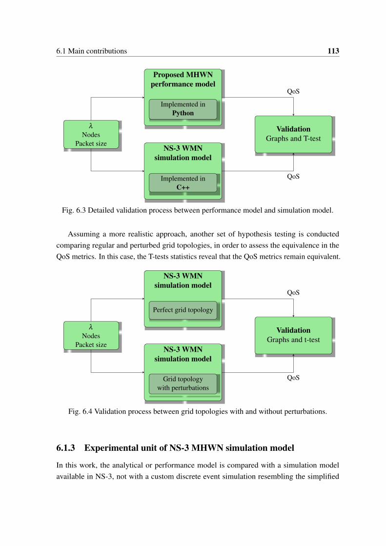
6.1 Main contributions 113
Proposed MHWNperformance model
Implemented inPython
λ
NodesPacket size NS-3 WMN
simulation model
Implemented inC++
ValidationGraphs and T-test
QoS
QoS
Fig. 6.3 Detailed validation process between performance model and simulation model.
Assuming a more realistic approach, another set of hypothesis testing is conductedcomparing regular and perturbed grid topologies, in order to assess the equivalence in theQoS metrics. In this case, the T-tests statistics reveal that the QoS metrics remain equivalent.
NS-3 WMNsimulation model
Perfect grid topology
λ
NodesPacket size NS-3 WMN
simulation model
Grid topologywith perturbations
ValidationGraphs and t-test
QoS
QoS
Fig. 6.4 Validation process between grid topologies with and without perturbations.
6.1.3 Experimental unit of NS-3 MHWN simulation model
In this work, the analytical or performance model is compared with a simulation modelavailable in NS-3, not with a custom discrete event simulation resembling the simplified
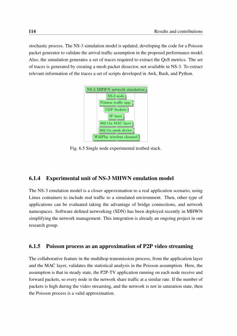
114 Results and contributions
stochastic process. The NS-3 simulation model is updated, developing the code for a Poissonpacket generator to validate the arrival traffic assumption in the proposed performance model.Also, the simulation generates a set of traces required to extract the QoS metrics. The setof traces is generated by creating a mesh packet dissector, not available in NS-3. To extractrelevant information of the traces a set of scripts developed in Awk, Bash, and Python.
NS-3 MHWN network simulation
NS-3 node
Poisson traffic app.
UDP Sockets
IP layer
802.11a MAC layer
802.11s mesh device
WifiPhy wireless channel
Fig. 6.5 Single node experimental testbed stack.
6.1.4 Experimental unit of NS-3 MHWN emulation model
The NS-3 emulation model is a closer approximation to a real application scenario, usingLinux containers to include real traffic to a simulated environment. Then, other type ofapplications can be evaluated taking the advantage of bridge connections, and networknamespaces. Software defined networking (SDN) has been deployed recently in MHWNsimplifying the network management. This integration is already an ongoing project in ourresearch group.
6.1.5 Poisson process as an approximation of P2P video streaming
The collaborative feature in the multihop transmission process, from the application layerand the MAC layer, validates the statistical analysis in the Poisson assumption. Here, theassumption is that in steady state, the P2P-TV application running on each node receive andforward packets, so every node in the network share traffic at a similar rate. If the number ofpackets is high during the video streaming, and the network is not in saturation state, thenthe Poisson process is a valid approximation.
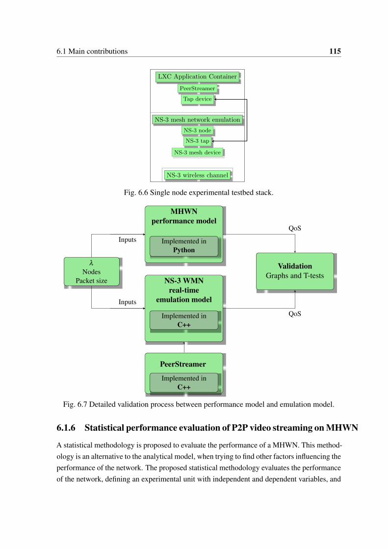
6.1 Main contributions 115
LXC Application Container
PeerStreamer
Tap device
NS-3 mesh network emulation
NS-3 node
NS-3 tap
NS-3 mesh device
NS-3 wireless channel
Fig. 6.6 Single node experimental testbed stack.
MHWNperformance model
Implemented inPython
Inputs
NS-3 WMNreal-time
emulation model
Implemented inC++
λ
NodesPacket size
Inputs
PeerStreamer
Implemented inC++
ValidationGraphs and T-tests
QoS
QoS
Fig. 6.7 Detailed validation process between performance model and emulation model.
6.1.6 Statistical performance evaluation of P2P video streaming on MHWN
A statistical methodology is proposed to evaluate the performance of a MHWN. This method-ology is an alternative to the analytical model, when trying to find other factors influencing theperformance of the network. The proposed statistical methodology evaluates the performanceof the network, defining an experimental unit with independent and dependent variables, and
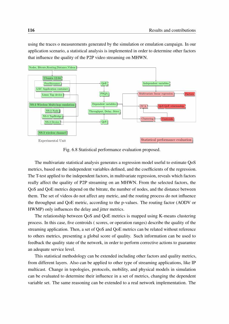
116 Results and contributions
using the traces o measurements generated by the simulation or emulation campaign. In ourapplication scenario, a statistical analysis is implemented in order to determine other factorsthat influence the quality of the P2P video streaming on MHWN.
Ubuntu 12.04
PeerStreamer QoE
PSQA
Nodes, Bitrate,Routing,Distance,Videos
Dependent variables
Independent variables
Multivariate linear regression
Clustering
PCA
Centroids
Factors
QoS-QoE relationship
Statistical performance evaluation
LXC Application container
Linux Tap device
NS-3 Wireless Multi-hop emulation
NS-3 Node
NS-3 TapBridge
NS-3 Device QoS
Throughput, Delay, Jitter
NS-3 wireless channel
Experimental Unit
Fig. 6.8 Statistical performance evaluation proposed.
The multivariate statistical analysis generates a regression model useful to estimate QoSmetrics, based on the independent variables defined, and the coefficients of the regression.The T-test applied to the independent factors, in multivariate regression, reveals which factorsreally affect the quality of P2P streaming on an MHWN. From the selected factors, theQoS and QoE metrics depend on the bitrate, the number of nodes, and the distance betweenthem. The set of videos do not affect any metric, and the routing process do not influencethe throughput and QoE metric, according to the p-values. The routing factor (AODV orHWMP) only influences the delay and jitter metrics.
The relationship between QoS and QoE metrics is mapped using K-means clusteringprocess. In this case, five centroids ( scores, or operation ranges) describe the quality of thestreaming application. Then, a set of QoS and QoE metrics can be related without referenceto others metrics, presenting a global score of quality. Such information can be used tofeedback the quality state of the network, in order to perform corrective actions to guaranteean adequate service level.
This statistical methodology can be extended including other factors and quality metrics,from different layers. Also can be applied to other type of streaming applications, like IPmulticast. Change in topologies, protocols, mobility, and physical models in simulationcan be evaluated to determine their influence in a set of metrics, changing the dependentvariable set. The same reasoning can be extended to a real network implementation. The
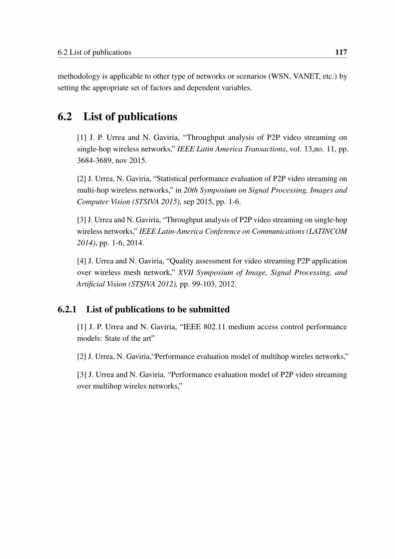
6.2 List of publications 117
methodology is applicable to other type of networks or scenarios (WSN, VANET, etc.) bysetting the appropriate set of factors and dependent variables.
6.2 List of publications
[1] J. P. Urrea and N. Gaviria, “Throughput analysis of P2P video streaming onsingle-hop wireless networks,” IEEE Latin America Transactions, vol. 13,no. 11, pp.3684-3689, nov 2015.
[2] J. Urrea, N. Gaviria, “Statistical performance evaluation of P2P video streaming onmulti-hop wireless networks,” in 20th Symposium on Signal Processing, Images andComputer Vision (STSIVA 2015), sep 2015, pp. 1-6.
[3] J. Urrea and N. Gaviria, “Throughput analysis of P2P video streaming on single-hopwireless networks,” IEEE Latin-America Conference on Communications (LATINCOM2014), pp. 1-6, 2014.
[4] J. Urrea and N. Gaviria, “Quality assessment for video streaming P2P applicationover wireless mesh network,” XVII Symposium of Image, Signal Processing, andArtificial Vision (STSIVA 2012), pp. 99-103, 2012.
6.2.1 List of publications to be submitted
[1] J. P. Urrea and N. Gaviria, “IEEE 802.11 medium access control performancemodels: State of the art”
[2] J. Urrea, N. Gaviria,“Performance evaluation model of multihop wireles networks,”
[3] J. Urrea and N. Gaviria, “Performance evaluation model of P2P video streamingover multihop wireles networks,”

References
[1] G. Hiertz, D. Denteneer, S. Max, R. Taori, J. Cardona, L. Berlemann, and B. Walke,“IEEE 802.11s: The WLAN Mesh Standard,” IEEE Wireless Communications, vol. 17,no. 1, pp. 104–111, feb 2010.
[2] J. Robinson and E. W. Knightly, “A performance study of deployment factors in wire-less mesh networks,” in IEEE INFOCOM 2007 - 26th IEEE International Conferenceon Computer Communications, 2007, pp. 2054–2062.
[3] G. Bianchi, “Performance Analysis of IEEE 802.11 Distributed CoordinationFunction,” IEEE Journal on Selected Areas in Communications, vol. 18, no. 3, pp.535–547, 2000.
[4] J. Mo, “Performance Modeling of Communication Networks with Markov Chains,”Synthesis Lectures on Communication Networks, vol. 3, no. 1, pp. 1–90, jan 2010.
[5] A. Kumar and E. Altman, “New insights from a fixed point analysis of single cellIEEE 802.11 WLANs,” IEEE/ACM Transactions on Networking (TON), vol. 15, no. 3,pp. 588 – 601, 2005.
[6] Q. Zhao, D. Tsang, and T. Sakurai, “A simple and approximate model for nonsaturatedIEEE 802.11 DCF,” Mobile Computing, IEEE Transactions on, vol. 8, no. 11, pp.1539–1553, 2009.
[7] A. Abbas, “Multihop Adjustment for the Number of Nodes in Contention-BasedMAC Protocols for Wireless Ad hoc Networks,” Computing Research Repository,arXiv:1108.4035v1[cs.NI], 2011.
[8] P. Stuckmann and R. Zimmermann, “European research on future internet design,”IEEE Wireless Communications, vol. 16, no. 5, pp. 14–22, 2009.
[9] Cisco, “The Zettabyte Era: Trends and Analysis,” 2015. [On-line]. Available: http://www.cisco.com/c/en/us/solutions/collateral/service-provider/visual-networking-index-vni/VNI_Hyperconnectivity_WP.pdf [Accessed: 2015-11-11]
[10] S. M. Thampi, “A Review on P2P Video Streaming,” arXiv:1304.1235 [cs.NI], pp.1–47, 2013.
[11] Y. Zhu, W. Zeng, H. Liu, Y. Guo, and S. Mathur, “Supporting video streamingservices in infrastructure wireless mesh networks: architecture and protocols,” in 2008IEEE International Conference on Communications. IEEE, 2008, pp. 1850–1855.
120 References
[12] T. Silverston, O. Fourmaux, A. Botta, A. Dainotti, A. Pescapé, G. Ventre, andK. Salamatian, “Traffic analysis of peer-to-peer IPTV communities,” ComputerNetworks, vol. 53, no. 4, pp. 470–484, 2009.
[13] “PPLive.” [Online]. Available: http://www.pptv.com/ [Accessed: 2014-05-13]
[14] “SopCast.” [Online]. Available: http://www.sopcast.org/ [Accessed: 2012-12-15]
[15] “AceStream.” [Online]. Available: http://acestreamguide.com/ [Accessed: 2013-01-20]
[16] “VideoWhisper.” [Online]. Available: http://www.videowhisper.com/ [Accessed:2015-01-20]
[17] “Tribler.” [Online]. Available: http://www.tribler.org/ [Accessed: 2014-03-23]
[18] “GoalBit.” [Online]. Available: http://www.goalbit-solutions.com/ [Accessed:2015-08-15]
[19] PeerStreamer, “Open source P2P Media Streaming.” [Online]. Available:http://peerstreamer.org/ [Accessed: 2015-06-11]
[20] H. Luo, S. Ci, and D. Wu, “A cross-layer optimized distributed scheduling algorithmfor peer-to-peer video streaming over multi-hop wireless mesh networks,” in 20096th Annual IEEE Communications Society Conference on Sensor, Mesh and Ad HocCommunications and Networks. IEEE, 2009, pp. 1–9.
[21] I. F. Akyildiz, X. Wang, and W. Wang, “Wireless mesh networks: a survey,” ComputerNetworks, vol. 47, no. 4, pp. 445–487, mar 2005.
[22] S. Sampaio, P. Souto, and F. Vasques, “A review of scalability and topological stabilityissues in IEEE 802.11s wireless mesh networks deployments,” International Journalof Communication Systems, vol. 26, pp. 671–693, 2016.
[23] S. Heimlicher, B. Plattner, S. Chandra Misra, S. Misra, and I. Woungang, Guide toWireless Mesh Networks, ser. Computer Communications and Networks, S. Misra,S. C. Misra, and I. Woungang, Eds. Springer-Verlag, 2009.
[24] S. Seth, A. Gankotiya, and A. Jindal, “Current State of Art Research Issues andChallenges in Wireless Mesh Networks,” 2010 Second International Conference onComputer Engineering and Applications, no. 978, pp. 199–203, 2010.
[25] H. Song, B. C. Kim, J. Y. Lee, and H. S. Lee, “IEEE 802.11-based Wireless MeshNetwork Testbed,” 2007 16th IST Mobile and Wireless Communications Summit, no.Mcl, pp. 1–5, jul 2007.
[26] R. C. Carrano, M. Bletsas, and L. C. S. Magalhães, “Mesh networks for digitalinclusion-testing OLPC’s XO mesh implementation,” published in InternationalSoftware Meet Porto Alegre, pp. 2–9, 2007.
[27] J. Ishmael, S. Bury, D. Pezaros, and N. Race, “Deploying Rural Community WirelessMesh Networks,” IEEE Internet Computing, vol. 12, no. 4, pp. 22–29, jul 2008.
References 121
[28] R. P. Karrer and A. Pescape, “2nd Generation Wireless Mesh Networks: Technical,Economical and Social Challenges,” Future Generation Communication andNetworking (FGCN 2007), pp. 262–267, dec 2007.
[29] B. Blywis, M. Guenes, F. Juraschek, and J. H. Schiller, “Trends, Advances, andChallenges in Testbed-based Wireless Mesh Network Research,” Mobile Networksand Applications, vol. 15, no. 3, pp. 315–329, feb 2010.
[30] P. H. Pathak and R. Dutta, “A Survey of Network Design Problems and Joint DesignApproaches in Wireless Mesh Networks,” IEEE Communications Surveys & Tutorials,vol. 13, no. 3, pp. 396–428, 2011.
[31] M. Afanasyev, T. Chen, G. M. Voelker, and A. C. Snoeren, “Usage patterns in anurban WiFi network,” IEEE/ACM Transactions on Networking, vol. 18, no. 5, pp.1359–1372, 2010.
[32] K. Ballantyne, W. Almuhtadi, and J. Melzer, “Autoconfiguration for faster WiFicommunity networks,” Proceedings of the 2015 IFIP/IEEE International Symposiumon Integrated Network Management, IM 2015, pp. 938–941, 2015.
[33] A. Ajayi, U. Roedig, C. Edwards, and N. Race, “A survey of rural Wireless MeshNetwork (WMN) deployments,” Proceedings, APWiMob 2014: IEEE Asia PacificConference on Wireless and Mobile 2014, pp. 119–125, 2014.
[34] V. Garg and K. Kataoka, “Performance Evaluation of Wireless Ad-hoc Network forPost-Disaster Recovery using Linux Live USB Nodes,” pp. 125–131, 2015.
[35] “MIT RoofNet, Central Square Roofnet.” [Online]. Available: http://pdos.csail.mit.edu/roofnet/doku.php [Accessed: 2013-03-03]
[36] “Berlin RoofNet Project.” [Online]. Available: http://sarwiki.informatik.hu-berlin.de/BerlinRoofNet [Accessed: 2016-06-03]
[37] “Freifunk.” [Online]. Available: http://start.freifunk.net/ [Accessed: 2016-05-05]
[38] “Funkfeuer free net.” [Online]. Available: http://www.funkfeuer.at/ [Accessed:2016-05-05]
[39] “Microsoft research - mesh connectivity layer.” [Online]. Available: http://research.microsoft.com/en-us/projects/mesh/ [Accessed: 2016-05-05]
[40] “Technology for All - Houston.” [Online]. Available: http://www.techforall.org[Accessed: 2013-02-11]
[41] “CUWiN. Cuwin - community wireless.” [Online]. Available: http://www.cuwireless.net/ [Accessed: 2012-11-11]
[42] A. Detti, C. Pisa, S. Salsano, and N. Blefari-Melazzi, “Wireless Mesh SoftwareDefined Networks (wmSDN),” International Conference on Wireless and MobileComputing, Networking and Communications, pp. 89–95, 2013.
[43] “University of California Santa Barbara, UCSB MeshNet.” [Online]. Available:http://moment.cs.ucsb.edu/meshnet/ [Accessed: 2010-05-05]
122 References
[44] “Purdue University: purdue university wireless mesh network testbed.” [Online].Available: https://engineering.purdue.edu/MESH [Accessed: 2016-05-05]
[45] “State University of New York at Stony Brook: hyacinth: an IEEE802.11-based multi-channel wireless mesh network.” [Online]. Available: http://www.ecsl.cs.sunysb.edu/multichannel/ [Accessed: 2016-06-05]
[46] P. De, A. Raniwala, S. Sharma, and T. Chiueh, “MiNT: a miniaturized network testbedfor mobile wireless research,” in Proceedings IEEE 24th Annual Joint Conference ofthe IEEE Computer and Communications Societies., vol. 4, mar 2005, pp. 2731–2742vol. 4.
[47] “Georgia Institute of Technology: broadband and wireless network (BWN) mesh.”[Online]. Available: http://www.ece.gatech.edu/research/labs/bwn/mesh/ [Accessed:2016-06-01]
[48] D. Raychaudhuri, I. Seskar, M. Ott, S. Ganu, K. Ramachandran, H. Kremo, R. Siracusa,H. Liu, and M. Singh, “Overview of the ORBIT radio grid testbed for evaluation ofnext-generation wireless network protocols,” in IEEE Wireless Communications andNetworking Conference, 2005, vol. 3, mar 2005, pp. 1664–1669 Vol. 3.
[49] K. Ramachandran, K. Almeroth, and E. M. Belding-Royer, “A framework for themanagement of large-scale wireless network testbeds.” in Proceedings of the 1stWorkshop on Wireless Network Measurements (WiNMee’05). 2005., 2005.
[50] “Mobile Communications Group (MCG), RA: ultra high-speed mobile informationand communication (UMIC) testbed.”
[51] H. Huang, P. Li, S. Guo, and W. Zhuang, “Software-defined wireless mesh networks:Architecture and traffic orchestration,” IEEE Network, vol. 29, no. 4, pp. 24–30, 2015.
[52] I. Brito, S. Gramacho, I. Ferreira, M. Nazare, L. Sampaio, and G. B. Figueiredo,“OpenWiMesh: A Framework for Software Defined Wireless Mesh Networks,” 2014Brazilian Symposium on Computer Networks and Distributed Systems, pp. 199–206,2014.
[53] D. Zhu, X. Yang, P. Zhao, and W. Yu, “Towards Effective Intra-Flow Network Cod-ing in Software Defined Wireless Mesh Networks,” Computer Communication andNetworks (ICCCN), 2015 24th International Conference on, pp. 1–8, 2015.
[54] A. V. Mamidi, S. Babu, and B. S. Manoj, “Dynamic Multi-hop Switch Handoffs inSoftware Defined Wireless Mesh Networks,” pp. 1–6, 2015.
[55] Y. Peng and L. Guo, “A Novel Hybrid Routing Forwarding Algorithm in SDNEnabled Wireless Mesh Networks,” in 2015 IEEE 17th International Conference onHigh Performance Computing and Communications (HPCC), 2015, pp. 1806–1811.
[56] “IEEE Standard for Information Technology–Telecommunications and information ex-change between systems–Local and metropolitan area networks–Specific requirementsPart 11: Wireless LAN Medium Access Control (MAC) and Physical Layer (PHY)specifications Am,” IEEE Std 802.11s-2011 (Amendment to IEEE Std 802.11-2007
References 123
as amended by IEEE 802.11k-2008, IEEE 802.11r-2008, IEEE 802.11y-2008, IEEE802.11w-2009, IEEE 802.11n-2009, IEEE 802.11p-2010, IEEE 802.11z-2010, IEEE802.11v-2011, and IEEE 802.11u-2011), pp. 1–372, 2011.
[57] R. C. Carrano, L. C. S. Magalhães, D. C. M. D. C. M. Saade, C. V. N. C. V. N.Albuquerque, and L. C. S. Magalhaes, “IEEE 802.11s Multihop MAC: A Tutorial,”IEEE Communications Surveys & Tutorials, vol. 13, no. 1, pp. 52–67, 2011.
[58] R. C. Carrano, D. C. M. Saade, M. E. M. Campista, and IM, “Multihop MAC: IEEE802.11 s Wireless Mesh Networks,” in Encyclopedia on Ad Hoc and UbiquitousComputing, 2008, ch. 19, p. 33.
[59] T. Imboden, K. Akkaya, and Z. Moore, “Performance evaluation of wireless meshnetworks using IEEE 802.11s and IEEE 802.11n,” Proceedings of ICC 2012, pp.5675–5679, 2012.
[60] “open80211s.” [Online]. Available: http://cozybit.com/open80211s/ [Accessed:2013-01-20]
[61] I. Armuelles-Voinov and J. Chung-Miranda, “Evaluation of QoS Provisioning inNodes of Wireless Mesh Networks based on IEEE,” in Proceddings of the 2014 IEEEcentral America and Panama convention (CONCAPAN XXXIV), 2014, pp. 1–5.
[62] Openwrt, “OLSR Mesh,” 2015. [Online]. Available: https://wiki.openwrt.org/doc/howto/mesh.olsr [Accessed: 2015-05-05]
[63] A. Barolli, T. Oda, L. Barolli, and M. Takizawa, “Experimental Results of a RaspberryPi and OLSR Based Wireless Content Centric Network Testbed ConsideringOpenWRT OS,” 2016 IEEE 30th International Conference on Advanced InformationNetworking and Applications (AINA), pp. 95–100, 2016.
[64] C. Palazzi, M. Brunati, and M. Roccetti, “An Openwrt solution for future wirelesshomes,” IEEE International Conference on Multimedia and Expo (ICME), pp. 1701–1706, 2010.
[65] I. Pratomo, A. Affandi, and D. Rahardjo, “OpenVoice: Low-cost mobile wirelesscommunication project for rural area based on OpenWRT,” International Seminar onIntelligent Technology and Its Applications (ISITIA), 2015, pp. 391–396, 2015.
[66] “Mikrotik Routers.” [Online]. Available: http://www.mikrotik.com/ [Accessed:2012-07-20]
[67] HP, “WLAN Mesh Technology Table of contents,” p. 13, 2014. [Online]. Available:http://h10032.www1.hp.com/ctg/Manual/c04497600 [Accessed: 2016-05-05]
[68] Fortinet, “FortiOS Handbook: Deploying Wireless Networks for FortiOS 5 . 0,”p. 113, 2014. [Online]. Available: http://docs.fortinet.com/uploaded/files/1091/fortigate-wireless-50.pdf [Accessed: 2016-05-05]
[69] Extreme Networks, “Extreme Wireless User Guide,” p. 630, 2016. [On-line]. Available: http://documentation.extremenetworks.com/wireless/UG/downloads/Wireless_User_Guide.pdf [Accessed: 2016-05-05]
124 References
[70] Aruba, “ARUBAOS: The operating system designed with scalable performance,”2014. [Online]. Available: http://www.arubanetworks.com/assets/ds/DS_AOS.pdf[Accessed: 2016-05-05]
[71] “Samsung Chord Library.” [Online]. Available: http://developer.samsung.com/resources/chord [Accessed: 2015-02-15]
[72] P. H. Pathak and R. Dutta, Designing for Network and Service Continuity in WirelessMesh Networks, 2013, vol. 2.
[73] D. Benyamina, A. Hafid, and M. Gendreau, “Wireless Mesh Networks Design - ASurvey,” IEEE Communications Surveys & Tutorials, vol. 14, no. 2, pp. 299–310,2012.
[74] S. Vural, D. Wei, and K. Moessner, “Survey of Experimental Evaluation Studies forWireless Mesh Network Deployments in Urban Areas Towards Ubiquitous Internet,”IEEE Communications Surveys & Tutorials, vol. 15, no. 1, pp. 223–239, 2013.
[75] J. Camp, J. Robinson, C. Steger, and E. Knightly, “Measurement driven deploymentof a two-tier urban mesh access network,” Proceedings of the 4th internationalconference on Mobile systems, applications and services - MobiSys 2006, p. 96, 2006.
[76] F. Li, Y. Wang, X.-Y. Li, A. Nusairat, and Y. Wu, “Gateway Placement for ThroughputOptimization in Wireless Mesh Networks,” Mobile Networks and Applications,vol. 13, no. 1-2, pp. 198–211, 2008.
[77] P. H. Pathak, R. Dutta, and P. Mohapatra, “On availability-performability tradeoff inwireless mesh networks,” IEEE Transactions on Mobile Computing, vol. 14, no. 3, pp.606–618, 2015.
[78] Cisco-Meraki, “Technologies: Mesh Routing,” 2016. [Online]. Available:https://meraki.cisco.com/technologies/mesh-routing [Accessed: 2016-08-05]
[79] Firetide, “A guide to wireless mesh networks,” 2015. [Online]. Available:http://www.firetide.com/blog/a-guide-to-wireless-mesh-networks/ [Accessed: 2016-05-08]
[80] Brocade, “Campus Network Infrastructure, Base Reference Architec-ture.” [Online]. Available: http://community.brocade.com/t5/Campus-Networks/Campus-Network-Infrastructure-Base-Reference-Architecture/ta-p/37419 [Accessed:2016-05-08]
[81] Rukus, “Smart WiFi for Higher Education.” [Online]. Available: http://uk.ruckuswireless.com/Smart-WiFi-Higher-Education [Accessed: 2016-05-08]
[82] B. Barekatain and M. Aizaini Maarof, “Video Streaming Over Wireless Mesh Net-works,” Journal of World’s Electrical Engineering and Technology, vol. 1, no. 1, pp.171–195, 2011.
[83] G. M. Sheeba and A. Nachiappan, “Implementation and Performance Evaluation inIeee 802 . 11S Based Campus Mesh Networks,” Indian Journal of Computer Scienceand Engineering (IJCSE), vol. 4, no. 1, pp. 29–33, 2013.
References 125
[84] G. Bolch, S. Greiner, H. de Meer, and K. Trivedi, Queueing Networks and MarkovChains: Modeling and Performance Evaluation with Computer Science Applications.John Wiley & Sons, Inc., mar 1998.
[85] R. Sadre, B. Haverkort, and P. Reinelt, “A fixed-point algorithm for closed queueingnetworks,” Formal Methods and Stochastic Models, 2007.
[86] A. Bobbio, M. Gribaudo, and M. Telek, “Analysis of large scale interacting systemsby mean field method,” QEST’08, pp. 1–10, 2008.
[87] O. Younes and N. Thomas, “Modelling and performance analysis of multi-hop ad hocnetworks,” Simulation Modelling Practice and Theory, vol. 38, pp. 69–97, nov 2013.
[88] M. S. Obaidat, “Fundamentals of Performance Evaluation of Computer andTelecommunications Systems,” 2009.
[89] H. Kobayashi, System Modeling and Analysis: Foundations of System PerformanceEvaluation. Pearson Addison Wesley, 2009.
[90] “IEEE Standard for Information technology-Telecommunications and information ex-change between systems-Local and metropolitan area networks-Specific requirements- Part 11: Wireless LAN Medium Access Control (MAC) and Physical Layer (PHY)Specifications,” ANSI/IEEE Std 802.11, 1999 Edition, vol. 1999, 1999.
[91] D. Moltchanov, “Performance models for wireless channels,” Computer ScienceReview, vol. 4, no. 3, pp. 153–184, 2010.
[92] O. Tickoo and B. Sikdar, “Modeling queueing and channel access delay in unsaturatedIEEE 802.11 random access MAC based wireless networks,” IEEE/ACM Transactionson Networking (TON), pp. 1–14, 2008.
[93] Q. Zhao, D. Tsang, and T. Sakurai, “Modeling nonsaturated IEEE 802.11 DCFnetworks utilizing an arbitrary buffer size,” IEEE Transactions on Mobile Computing,vol. 10, no. 9, pp. 1248–1263, 2011.
[94] D. G. Duffy, Advanced engineering mathematics with MATLAB. CRC Press, 2010.
[95] A. Misra, T. Ott, and J. Baras, “The window distribution of multiple TCPs with randomloss queues,” in Global Telecommunications Conference, 1999. GLOBECOM ’99,vol. 3, 1999, pp. 1714–1726 vol.3.
[96] C. Casetti and M. Meo, “An analytical framework for the performance evaluation ofTCP Reno connections,” Computer Networks, vol. 37, no. 5, pp. 669–682, 2001.
[97] V. Firoiu and M. Borden, “A study of active queue management for congestion control,”in IEEE INFOCOM 2000. Nineteenth Annual Joint Conference of the IEEE Computerand Communications Societies. Proceedings., vol. 3, mar 2000, pp. 1435–1444 vol.3.
[98] A. Kumar, D. Manjunath, and J. Kuri, Communication networking: an analyticalapproach. Morgan Kaufmann Publishers, 2004.
[99] W. Whitt, “Decomposition approximations for time-dependent Markovian queueingnetworks,” Operations Research Letters, vol. 24, pp. 97–103, 1999.
126 References
[100] K. A. Alnowibet and H. Perros, “Nonstationary analysis of the loss queue and ofqueueing networks of loss queues,” European Journal of Operational Research, vol.196, no. 3, pp. 1015–1030, aug 2009.
[101] D. Moltchanov and R. Dunaytsev, “Modeling TCP performance over wireless channelsusing fixed-point approximation,” in International Conference on Telecommunications,2008. ICT 2008., jun 2008, pp. 1–10.
[102] A. Wierman and T. Osogami, “A unified framework for modeling TCP-Vegas, TCP-SACK, and TCP-Reno,” in 11th IEEE/ACM International Symposium on Modeling,Analysis and Simulation of Computer Telecommunications Systems, 2003. MASCOTS2003., oct 2003, pp. 269–278.
[103] I. Tinnirello, G. Bianchi, and Y. Xiao, “Refinements on IEEE 802.11 distributedcoordination function modeling approaches,” Vehicular Technology, IEEE, vol. 59,no. 3, pp. 1055–1067, 2010.
[104] K. Duffy, D. W. Malone, and D. J. Leith, “Modelling 802.11 wireless links,” in44th IEEE Conference on Decision and Control, 2005 and 2005 European ControlConference. CDC-ECC’05. IEEE, 2006, pp. 6952–6957.
[105] O. Tickoo and B. Sikdar, “Queueing analysis and delay mitigation in IEEE 802.11random access MAC based wireless networks,” in INFOCOM 2004. Twenty-thirdannualjoint conference of the IEEE computer and communications societies, vol. 2.IEEE, 2004, pp. 1404–1413.
[106] Y. Tay and K. Chua, “A capacity analysis for the IEEE 802.11 MAC protocol,”Wireless networks, pp. 159–171, 2001.
[107] M. Ozdemir and A. McDonald, “On the performance of ad hoc wireless LANs: Apractical queuing theoretic model,” Performance Evaluation, vol. 63, no. 11, pp.1127–1156, nov 2006.
[108] H. Zhai, Y. Kwon, and Y. Fang, “Performance analysis of IEEE 802.11 MACprotocols in wireless LANs,” Wireless Communications and Mobile Computing,vol. 4, no. 8, pp. 917–931, dec 2004.
[109] Y. Zheng, K. Lu, D. Wu, and Y. Fang, “Performance analysis of IEEE 802.11 DCF inimperfect channels,” IEEE Transactions on Vehicular Technology, vol. 55, no. 5, pp.1648–1656, 2006.
[110] F. Alizadeh-Shabdiz and S. Subramaniam, “Analytical Models for Single-Hop andMulti-Hop Ad Hoc Networks,” Mobile Networks and Applications, vol. 11, no. 1, pp.75–90, dec 2005.
[111] Q. Zhao, D. Tsang, and T. Sakurai, “A simple and approximate model for nonsaturatedIEEE 802.11 DCF,” IEEE Transactions on Mobile Computing, vol. 8, no. 11, pp.1539–1553, 2009.
[112] J. Jin, J. Gubbi, S. Marusic, and M. Palaniswami, “An Information Framework forCreating a Smart City Through Internet of Things,” IEEE Internet of Things Journal,vol. 1, no. 2, pp. 112–121, 2014.
References 127
[113] M. Conti and S. Giordano, “Mobile ad hoc networking: Milestones, challenges, andnew research directions,” IEEE Communications Magazine, vol. 52, no. 1, pp. 85–96,2014.
[114] M. Hira, F. Tobagi, and K. Medepalli, “Throughput analysis of a path in an IEEE802.11 multihop wireless network,” Wireless Communications and NetworkingConference, 2007.WCNC 2007. IEEE, pp. 441–446, 2007.
[115] L. Xie, H. Wang, G. Wei, and Z. Xie, “Performance Analysis of IEEE 802.11 DCF inMulti-hop Ad Hoc Networks,” 2009 International Conference on Networks Security,Wireless Communications and Trusted Computing, pp. 227–230, apr 2009.
[116] L. T. Nguyen, R. Beuran, and Y. Shinoda, “Performance analysis of IEEE 802.11 inmulti-hop wireless networks,” in Proceedings of the 3rd international conference onMobile ad-hoc and sensor networks. Springer-Verlag, 2007, pp. 326–337.
[117] K. Duffy, D. Malone, and D. J. Leith, “Modeling the 802.11 distributed coordinationfunction in non-saturated conditions,” IEEE Communications Letters, vol. 9, no. 8, pp.715–717, aug 2005.
[118] M. Carvalho and J. Garcia-Luna-Aceves, “A scalable model for channel accessprotocols in multihop ad hoc networks,” Proceedings of the 10th annual internationalconference on Mobile computing and networking, pp. 330–344, 2004.
[119] A. Abdullah, F. Gebali, and L. Cai, “Modeling the throughput and delay inwireless multihop ad hoc networks,” IEEE Global Telecommunications Conference,GLOBECOM., pp. 1–6, 2009.
[120] E. Ghadimi, a. Khonsari, a. Diyanat, M. Farmani, and N. Yazdani, “An analyticalmodel of delay in multi-hop wireless ad hoc networks,” Wireless Networks, jul 2011.
[121] K. Medepalli and F. a. Tobagi, “Towards Performance Modeling of IEEE 802.11Based Wireless Networks: A Unified Framework and Its Applications,” ProceedingsIEEE INFOCOM 2006. 25TH IEEE International Conference on ComputerCommunications, vol. 00, no. c, pp. 1–12, apr 2006.
[122] J. Zhou and K. Mitchell, “A scalable delay based analytical framework for CSMA/CAwireless mesh networks,” Computer Networks, vol. 54, no. 2, pp. 304–318, feb 2010.
[123] A. Alshanyour and A. Agarwal, “Throughput analysis for IEEE 802.11 in multi-hopwireless networks,” Communications (ICC), 2012 IEEE, no. 1, pp. 291–295, 2012.
[124] A. Abbas and K. Soufy, “Analysis of IEEE 802.11 DCF for ad hoc networks:Saturation,” (IMSAA), 2011 IEEE 5th, 2011.
[125] A. M. Abbas, K. Abdullah, and M. Al, “Analysis of IEEE 802 .11 DCF for AdHoc Networks Under Nonsaturation Conditions,” Proceedings of the InternationalConference on Advances in Computing, Communications and Informatics, pp. 392–398, 2012.

128 References
[126] S. Pourmohammad, R. Soosahabi, D. Perkins, and A. Fekih, “An Analytical QoSModel for IEEE 802 .11-based Single and Multihop Wireless Networks,” InternationalConference on Computing, Networking and Communications (ICNC), 2014, pp. 914–920, 2014.
[127] S. a. Alabady, M. F. M. Salleh, and A. Hasib, “Throughput and Delay Analysis ofIEEE 802.11 DCF in the Presence of Hidden Nodes for Multi-hop Wireless Networks,”Wireless Personal Communications, jun 2014.
[128] E. Winands, T. Denteneer, J. Resing, and R. Rietman, “A finite-source feedbackqueueing network as a model for the IEEE 802.11 DCF,” European Transaction onTelecommunication, vol. 16, no. 1, pp. 77–89, 2005.
[129] H. C. Tijms, A First Course in Stochastic Models. John Wiley & Sons, Ltd, mar2003.
[130] D. Gross, J. Shortle, J. Thompson, and C. Harris, Fundamentals of queueing theory.John Wiley & Sons, 2008.
[131] W. Feller, An introduction to probability theory and its applications, 3rd ed. Wiley,1968, vol. I.
[132] O. C. Ibe, Markov Processes for Stochastic Modeling, 2nd ed. Elsevier, 2013.
[133] V. Karyotis, E. Stai, and S. Papavassiliou, Evolutionary Dynamics of ComplexCommunications Networks. CRC Press, 2014.
[134] S. Basagni, M. Conti, S. Giordano, and I. Stojmenovic, Mobile ad hoc networking:Cutting edge directions. Wiley, 2013.
[135] O. Ibe, Fundamentals of stochastic networks, 2011.
[136] A. Webb, Statistical pattern recognition. John Wiley & Sons, Ltd, 2011.
[137] S. P. Borgatti, “Centrality and network flow,” Social Networks, vol. 27, no. 1, pp.55–71, jan 2005.
[138] D. Arrowsmith, R. Mondrag, and M. Woolf, “Data traffic, topology and congestion,”in Complex Dynamics in Communication Networks. Springer Berlin Heidelberg,2005, pp. 1–29.
[139] U. Brandes, “A faster algorithm for betweenness centrality,” The Journal of Mathe-matical Sociology, vol. 25, no. 2, pp. 163–177, 2001.
[140] K. Wehrle and J. Gross, Modeling and tools for network simulation. Springer, 2010.
[141] L. Zhao, Y.-C. Lai, K. Park, and N. Ye, “Onset of traffic congestion in complexnetworks,” Physical Review E, vol. 71, no. 2, p. 026125, feb 2005.
[142] K. Andreev and P. Boyko, “IEEE 802.11 s Mesh Networking NS-3 Model,” Workshopon NS-3, WNS3 2010, p. 43, 2010.
References 129
[143] P. D. Iseger, “Numerical transform inversion using Gaussian quadrature,” Probabilityin the Engineering and Informational Sciences, no. 20, pp. 1–44, 2006.
[144] N. Nechval, K. Nechval, V. Danovich, and N. Ribakova, “Statistical Techniquesfor Validation of Simulation and Analytic Stochastic Models,” in Analytical andStochastic Modeling Techniques and Applications: 21st International Conference,ASMTA 2014., B. Sericola, M. Telek, and G. Horváth, Eds. Cham: SpringerInternational Publishing, 2014, pp. 155–169.
[145] W. Navidi, Statistics for Engineers and Scientists, 4th ed. McGraw-Hill, 2015.
[146] J. Urrea and N. Gaviria, “Quality assessment for video streaming P2P applicationover wireless mesh network,” XVII Symposium of Image, Signal Processing, andArtificial Vision (STSIVA 2012), pp. 99–103, 2012.
[147] R. Jain and S. Routhier, “Packet trains–measurements and a new model for computernetwork traffic,” JSAC, IEEE Journal on selected areas in communications,, pp.986–995, 1986.
[148] D. G. Feitelson, Workload Modeling for Computer Systems Performance Evaluation.Cambridge University Press, 2014.
[149] M. Venkataraman, M. Chatterjee, and S. Chattopadhyay, “Evaluating Quality ofExperience for Streaming Video in Real Time,” GLOBECOM 2009 - 2009 IEEEGlobal Telecommunications Conference, pp. 1–6, nov 2009.
[150] Y. Chen, K. Wu, and Q. Zhang, “From QoS to QoE : A Tutorial on Video QualityAssessment,” IEEE Communications Surveys & Tutorials,, vol. 17, no. 2, pp. 1126–1165, 2015.
[151] S. Chikkerur, V. Sundaram, M. Reisslein, and L. J. Karam, “Objective video qualityassessment methods: A classification, review, and performance comparison,” IEEETransactions on Broadcasting, vol. 57, no. 2 PART 1, pp. 165–182, 2011.
[152] G. Rubino, M. Varela, and J.-M. Bonnin, “Controlling Multimedia QoS in the FutureHome Network Using the PSQA Metric,” The Computer Journal, vol. 49, no. 2, dec2006.
[153] C. Ke and C. Shieh, “An evaluation framework for more realistic simulations ofMPEG video transmission,” Journal of information, vol. 440, pp. 425–440, 2008.
[154] N. De León, “Evaluación de calidad de video en una aplicación P2P: Goalbit,” MasterThesis, Universidad de la República de Uruguay, 2010.
[155] S. Mohamed, S. Member, and G. Rubino, “A study of real-time packet video qualityusing random neural networks,” IEEE Trans. on Circuits and Systems for Videotechnology, vol. 12, no. 12, pp. 1071–1083, 2002.
[156] K. Piamrat, C. Viho, J.-M. Bonnin, and A. Ksentini, “Quality of ExperienceMeasurements for Video Streaming over Wireless Networks,” 2009 Sixth InternationalConference on Information Technology: New Generations, pp. 1184–1189, 2009.
130 References
[157] G. Rubino, “Quantifying the quality of audio and video transmissions over theInternet: the PSQA approach,” Design and operations of communication networks: a,2005.
[158] P. Rodriguez-Bocca, “Quality-centric design of Peer-to-Peer systems for live-videobroadcasting,” Ph.D. dissertation, Université de Rennes, 2008.
[159] A. Malik, J. Qadir, B. Ahmad, K.-L. Alvin Yau, and U. Ullah, “QoS in IEEE 802.11-based Wireless Networks: A Contemporary Survey,” Journal of Network and Com-puter Applications, vol. 55, no. 6, pp. 24–46, 2015.
[160] M. Alreshoodi and J. Woods, “Survey on QoE\QoS Correlation Models forMultimedia Services,” International Journal of Distributed and Parallel systems,vol. 4, no. 3, pp. 53–72, 2013.
[161] R. Mok, E. Chan, and R. Chang, “Measuring the quality of experience of HTTP videostreaming,” Integrated Network Management (IM), 2011 IFIP/IEEE InternationalSymposium on, pp. 485–492, 2011.
[162] H. Du, C. Guo, and Y. Liu, “Research on relationship between QoE and QoS based onBP Neural Network,” Network Infrastructure and Digital, Proceedings of, 2009.
[163] D. Tobón and N. Gaviria, “Analysis of quality of service metrics for CSMA / CAprotocol configuration in wireless body area networks,” Ingeniería y Desarrollo,vol. 30, no. 1, p. 24, 2012.
[164] J. M. Dricot, P. De Doncker, and E. Zimànyi, “Multivariate Analysis of theCross-Layer Interaction in Wireless Networks Simulations,” in Proc. of InternationalWorkshop on Wireless Ad-hoc Networks, IWWAN, 2005.
[165] J. Bustos-Jiménez, R. Alonso, C. Faundez, and H. Meric, “Boxing experience:Measuring QoS and QoE of multimedia streaming using NS3, LXC and VLC,” LocalComputer Networks Workshops (LCN Workshops), 2014 IEEE 39th Conference on,pp. 658–662, 2014.
[166] D. T. Pham, S. S. Dimov, and C. D. Nguyen, “Selection of K in K-meansclustering,” Proceedings of the Institution of Mechanical Engineers, Part C: Journalof Mechanical Engineering Science, vol. 219, no. 1, pp. 103–119, jan 2005.
[167] EMC, Data Science and Big Data Analytics. John Wiley & Sons Inc., 2015.
[168] L. Abeni, A. Bakay, and R. Birke, “WineStreamer(s): Flexible P2P-TV StreamingApplications,” in IEEE Conference on Computer Communications Workshops,INFOCOM 2011, Shanghai, China, 2011, pp. 5–6.
[169] P. Teetor, R Cookbook. O’Reilly Media, 2011.
[170] J. Farjo, R. A. Assi, W. Masri, and F. Zaraket, “Does Principal Component AnalysisImprove Cluster-Based Analysis?” 2013 IEEE Sixth International Conference onSoftware Testing, Verification and Validation Workshops, mar 2013.
[171] J. Shlens, “A Tutorial on Principal Component Analysis,” CoRR abs/1404.1100, apr2014.

Appendix A
Statistical validation tables
A.1 Throughput
Table A.1 Percentage of accepted H0 for Throughput (AODV).
λ Packet Size p-values > 0.05
10 64 100%
10 256 100%
10 512 100%
10 1024 100%
50 64 60%
50 256 100%
50 512 100%
50 1024 100%
100 64 100%
100 256 100%
100 512 100%
100 1024 100%
150 64 100%
150 256 100%
150 512 100%
150 1024 100%
200 64 100%
200 256 100%
200 512 100%
200 1024 100%
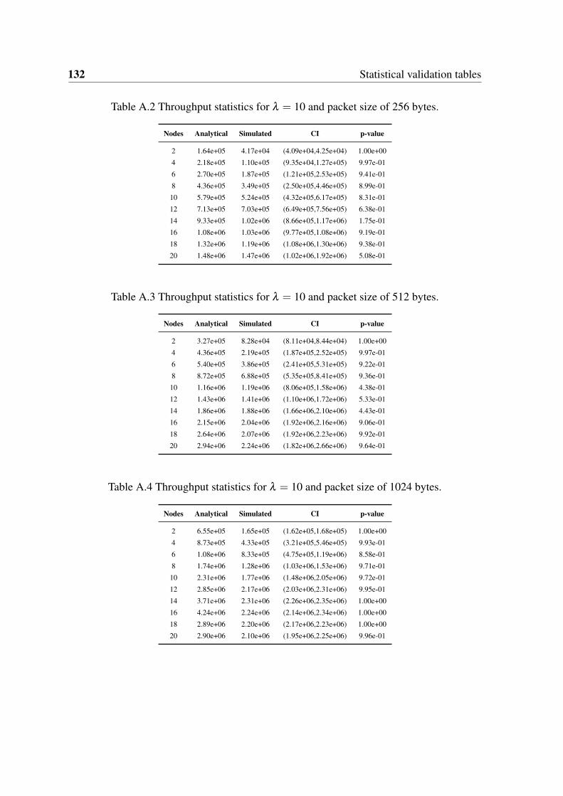
132 Statistical validation tables
Table A.2 Throughput statistics for λ = 10 and packet size of 256 bytes.
Nodes Analytical Simulated CI p-value
2 1.64e+05 4.17e+04 (4.09e+04,4.25e+04) 1.00e+00
4 2.18e+05 1.10e+05 (9.35e+04,1.27e+05) 9.97e-01
6 2.70e+05 1.87e+05 (1.21e+05,2.53e+05) 9.41e-01
8 4.36e+05 3.49e+05 (2.50e+05,4.46e+05) 8.99e-01
10 5.79e+05 5.24e+05 (4.32e+05,6.17e+05) 8.31e-01
12 7.13e+05 7.03e+05 (6.49e+05,7.56e+05) 6.38e-01
14 9.33e+05 1.02e+06 (8.66e+05,1.17e+06) 1.75e-01
16 1.08e+06 1.03e+06 (9.77e+05,1.08e+06) 9.19e-01
18 1.32e+06 1.19e+06 (1.08e+06,1.30e+06) 9.38e-01
20 1.48e+06 1.47e+06 (1.02e+06,1.92e+06) 5.08e-01
Table A.3 Throughput statistics for λ = 10 and packet size of 512 bytes.
Nodes Analytical Simulated CI p-value
2 3.27e+05 8.28e+04 (8.11e+04,8.44e+04) 1.00e+00
4 4.36e+05 2.19e+05 (1.87e+05,2.52e+05) 9.97e-01
6 5.40e+05 3.86e+05 (2.41e+05,5.31e+05) 9.22e-01
8 8.72e+05 6.88e+05 (5.35e+05,8.41e+05) 9.36e-01
10 1.16e+06 1.19e+06 (8.06e+05,1.58e+06) 4.38e-01
12 1.43e+06 1.41e+06 (1.10e+06,1.72e+06) 5.33e-01
14 1.86e+06 1.88e+06 (1.66e+06,2.10e+06) 4.43e-01
16 2.15e+06 2.04e+06 (1.92e+06,2.16e+06) 9.06e-01
18 2.64e+06 2.07e+06 (1.92e+06,2.23e+06) 9.92e-01
20 2.94e+06 2.24e+06 (1.82e+06,2.66e+06) 9.64e-01
Table A.4 Throughput statistics for λ = 10 and packet size of 1024 bytes.
Nodes Analytical Simulated CI p-value
2 6.55e+05 1.65e+05 (1.62e+05,1.68e+05) 1.00e+00
4 8.73e+05 4.33e+05 (3.21e+05,5.46e+05) 9.93e-01
6 1.08e+06 8.33e+05 (4.75e+05,1.19e+06) 8.58e-01
8 1.74e+06 1.28e+06 (1.03e+06,1.53e+06) 9.71e-01
10 2.31e+06 1.77e+06 (1.48e+06,2.05e+06) 9.72e-01
12 2.85e+06 2.17e+06 (2.03e+06,2.31e+06) 9.95e-01
14 3.71e+06 2.31e+06 (2.26e+06,2.35e+06) 1.00e+00
16 4.24e+06 2.24e+06 (2.14e+06,2.34e+06) 1.00e+00
18 2.89e+06 2.20e+06 (2.17e+06,2.23e+06) 1.00e+00
20 2.90e+06 2.10e+06 (1.95e+06,2.25e+06) 9.96e-01
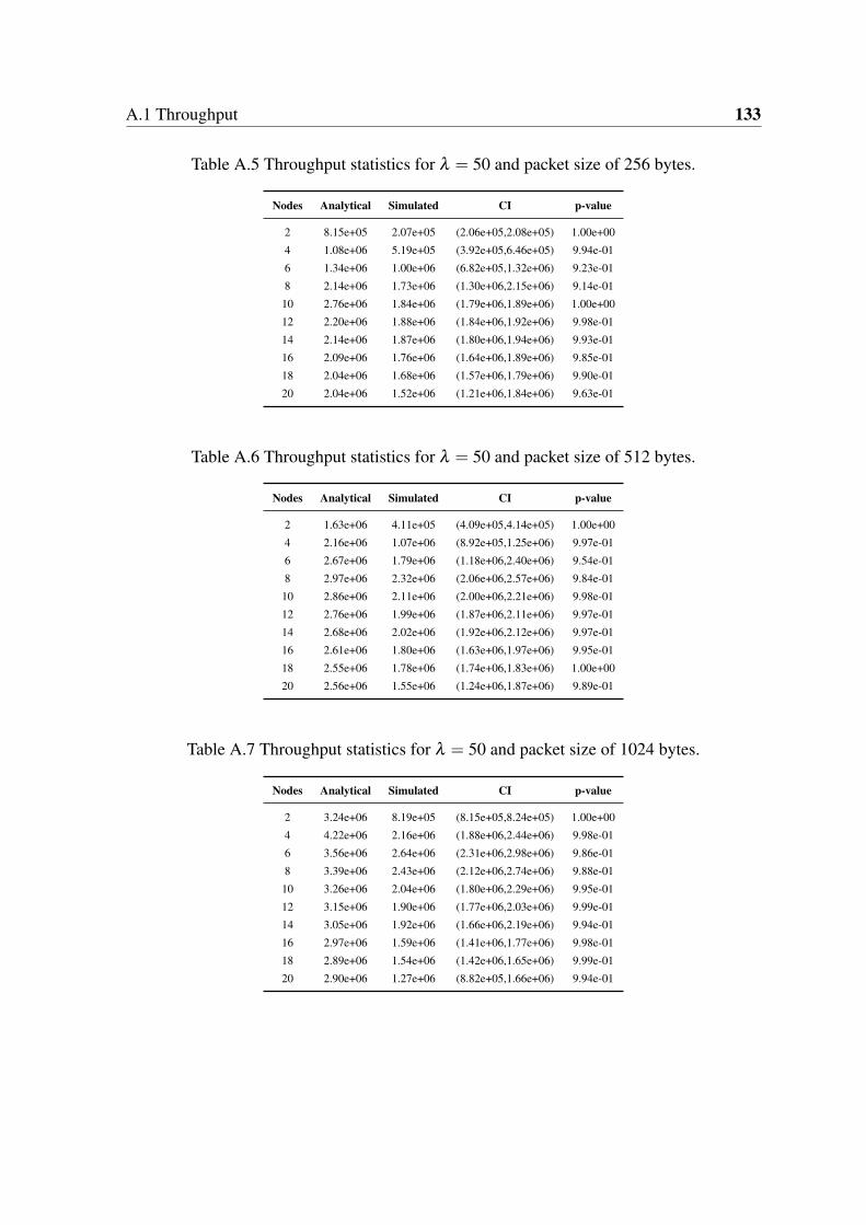
A.1 Throughput 133
Table A.5 Throughput statistics for λ = 50 and packet size of 256 bytes.
Nodes Analytical Simulated CI p-value
2 8.15e+05 2.07e+05 (2.06e+05,2.08e+05) 1.00e+00
4 1.08e+06 5.19e+05 (3.92e+05,6.46e+05) 9.94e-01
6 1.34e+06 1.00e+06 (6.82e+05,1.32e+06) 9.23e-01
8 2.14e+06 1.73e+06 (1.30e+06,2.15e+06) 9.14e-01
10 2.76e+06 1.84e+06 (1.79e+06,1.89e+06) 1.00e+00
12 2.20e+06 1.88e+06 (1.84e+06,1.92e+06) 9.98e-01
14 2.14e+06 1.87e+06 (1.80e+06,1.94e+06) 9.93e-01
16 2.09e+06 1.76e+06 (1.64e+06,1.89e+06) 9.85e-01
18 2.04e+06 1.68e+06 (1.57e+06,1.79e+06) 9.90e-01
20 2.04e+06 1.52e+06 (1.21e+06,1.84e+06) 9.63e-01
Table A.6 Throughput statistics for λ = 50 and packet size of 512 bytes.
Nodes Analytical Simulated CI p-value
2 1.63e+06 4.11e+05 (4.09e+05,4.14e+05) 1.00e+00
4 2.16e+06 1.07e+06 (8.92e+05,1.25e+06) 9.97e-01
6 2.67e+06 1.79e+06 (1.18e+06,2.40e+06) 9.54e-01
8 2.97e+06 2.32e+06 (2.06e+06,2.57e+06) 9.84e-01
10 2.86e+06 2.11e+06 (2.00e+06,2.21e+06) 9.98e-01
12 2.76e+06 1.99e+06 (1.87e+06,2.11e+06) 9.97e-01
14 2.68e+06 2.02e+06 (1.92e+06,2.12e+06) 9.97e-01
16 2.61e+06 1.80e+06 (1.63e+06,1.97e+06) 9.95e-01
18 2.55e+06 1.78e+06 (1.74e+06,1.83e+06) 1.00e+00
20 2.56e+06 1.55e+06 (1.24e+06,1.87e+06) 9.89e-01
Table A.7 Throughput statistics for λ = 50 and packet size of 1024 bytes.
Nodes Analytical Simulated CI p-value
2 3.24e+06 8.19e+05 (8.15e+05,8.24e+05) 1.00e+00
4 4.22e+06 2.16e+06 (1.88e+06,2.44e+06) 9.98e-01
6 3.56e+06 2.64e+06 (2.31e+06,2.98e+06) 9.86e-01
8 3.39e+06 2.43e+06 (2.12e+06,2.74e+06) 9.88e-01
10 3.26e+06 2.04e+06 (1.80e+06,2.29e+06) 9.95e-01
12 3.15e+06 1.90e+06 (1.77e+06,2.03e+06) 9.99e-01
14 3.05e+06 1.92e+06 (1.66e+06,2.19e+06) 9.94e-01
16 2.97e+06 1.59e+06 (1.41e+06,1.77e+06) 9.98e-01
18 2.89e+06 1.54e+06 (1.42e+06,1.65e+06) 9.99e-01
20 2.90e+06 1.27e+06 (8.82e+05,1.66e+06) 9.94e-01
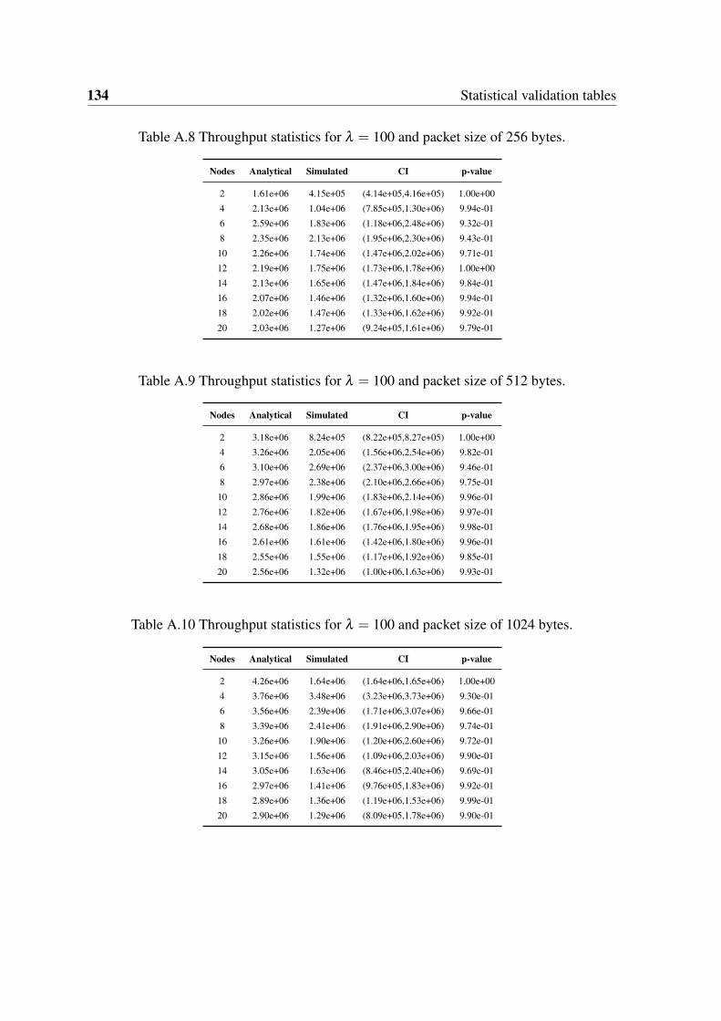
134 Statistical validation tables
Table A.8 Throughput statistics for λ = 100 and packet size of 256 bytes.
Nodes Analytical Simulated CI p-value
2 1.61e+06 4.15e+05 (4.14e+05,4.16e+05) 1.00e+00
4 2.13e+06 1.04e+06 (7.85e+05,1.30e+06) 9.94e-01
6 2.59e+06 1.83e+06 (1.18e+06,2.48e+06) 9.32e-01
8 2.35e+06 2.13e+06 (1.95e+06,2.30e+06) 9.43e-01
10 2.26e+06 1.74e+06 (1.47e+06,2.02e+06) 9.71e-01
12 2.19e+06 1.75e+06 (1.73e+06,1.78e+06) 1.00e+00
14 2.13e+06 1.65e+06 (1.47e+06,1.84e+06) 9.84e-01
16 2.07e+06 1.46e+06 (1.32e+06,1.60e+06) 9.94e-01
18 2.02e+06 1.47e+06 (1.33e+06,1.62e+06) 9.92e-01
20 2.03e+06 1.27e+06 (9.24e+05,1.61e+06) 9.79e-01
Table A.9 Throughput statistics for λ = 100 and packet size of 512 bytes.
Nodes Analytical Simulated CI p-value
2 3.18e+06 8.24e+05 (8.22e+05,8.27e+05) 1.00e+00
4 3.26e+06 2.05e+06 (1.56e+06,2.54e+06) 9.82e-01
6 3.10e+06 2.69e+06 (2.37e+06,3.00e+06) 9.46e-01
8 2.97e+06 2.38e+06 (2.10e+06,2.66e+06) 9.75e-01
10 2.86e+06 1.99e+06 (1.83e+06,2.14e+06) 9.96e-01
12 2.76e+06 1.82e+06 (1.67e+06,1.98e+06) 9.97e-01
14 2.68e+06 1.86e+06 (1.76e+06,1.95e+06) 9.98e-01
16 2.61e+06 1.61e+06 (1.42e+06,1.80e+06) 9.96e-01
18 2.55e+06 1.55e+06 (1.17e+06,1.92e+06) 9.85e-01
20 2.56e+06 1.32e+06 (1.00e+06,1.63e+06) 9.93e-01
Table A.10 Throughput statistics for λ = 100 and packet size of 1024 bytes.
Nodes Analytical Simulated CI p-value
2 4.26e+06 1.64e+06 (1.64e+06,1.65e+06) 1.00e+00
4 3.76e+06 3.48e+06 (3.23e+06,3.73e+06) 9.30e-01
6 3.56e+06 2.39e+06 (1.71e+06,3.07e+06) 9.66e-01
8 3.39e+06 2.41e+06 (1.91e+06,2.90e+06) 9.74e-01
10 3.26e+06 1.90e+06 (1.20e+06,2.60e+06) 9.72e-01
12 3.15e+06 1.56e+06 (1.09e+06,2.03e+06) 9.90e-01
14 3.05e+06 1.63e+06 (8.46e+05,2.40e+06) 9.69e-01
16 2.97e+06 1.41e+06 (9.76e+05,1.83e+06) 9.92e-01
18 2.89e+06 1.36e+06 (1.19e+06,1.53e+06) 9.99e-01
20 2.90e+06 1.29e+06 (8.09e+05,1.78e+06) 9.90e-01

A.1 Throughput 135
Table A.11 Throughput statistics for λ = 200 and packet size of 256 bytes.
Nodes Analytical Simulated CI p-value
2 2.80e+06 8.32e+05 (8.30e+05,8.34e+05) 1.00e+00
4 2.56e+06 2.20e+06 (1.63e+06,2.78e+06) 8.39e-01
6 2.45e+06 2.48e+06 (2.36e+06,2.60e+06) 3.27e-01
8 2.35e+06 2.13e+06 (1.90e+06,2.36e+06) 9.05e-01
10 2.26e+06 1.92e+06 (1.78e+06,2.07e+06) 9.81e-01
12 2.19e+06 1.65e+06 (1.50e+06,1.80e+06) 9.91e-01
14 2.13e+06 1.74e+06 (1.42e+06,2.05e+06) 9.39e-01
16 2.07e+06 1.45e+06 (1.36e+06,1.55e+06) 9.97e-01
18 2.02e+06 1.35e+06 (1.06e+06,1.64e+06) 9.80e-01
20 2.03e+06 1.25e+06 (9.85e+05,1.52e+06) 9.87e-01
Table A.12 Throughput statistics for λ = 200 and packet size of 512 bytes.
Nodes Analytical Simulated CI p-value
2 3.63e+06 1.65e+06 (1.65e+06,1.66e+06) 1.00e+00
4 3.26e+06 3.71e+06 (3.11e+06,4.31e+06) 1.28e-01
6 3.10e+06 2.80e+06 (2.45e+06,3.15e+06) 8.92e-01
8 2.97e+06 2.37e+06 (1.90e+06,2.84e+06) 9.41e-01
10 2.86e+06 2.40e+06 (2.07e+06,2.72e+06) 9.52e-01
12 2.76e+06 1.88e+06 (1.49e+06,2.28e+06) 9.79e-01
14 2.68e+06 1.94e+06 (1.56e+06,2.31e+06) 9.73e-01
16 2.61e+06 1.51e+06 (1.21e+06,1.81e+06) 9.92e-01
18 2.55e+06 1.55e+06 (1.14e+06,1.97e+06) 9.81e-01
20 2.56e+06 1.25e+06 (7.70e+05,1.74e+06) 9.85e-01
Table A.13 Throughput statistics for λ = 200 and packet size of 1024 bytes.
Nodes Analytical Simulated CI p-value
2 1.31e+07 3.29e+06 (3.28e+06,3.30e+06) 1.00e+00
4 3.78e+06 4.20e+06 (3.89e+06,4.52e+06) 5.16e-02
6 3.57e+06 3.01e+06 (2.00e+06,4.00e+06) 8.23e-01
8 3.41e+06 3.04e+06 (2.40e+06,3.68e+06) 8.23e-01
10 3.28e+06 2.47e+06 (1.78e+06,3.16e+06) 9.34e-01
12 3.17e+06 1.93e+06 (1.72e+06,2.15e+06) 9.97e-01
14 3.07e+06 2.10e+06 (1.74e+06,2.46e+06) 9.85e-01
16 2.99e+06 1.75e+06 (1.20e+06,2.31e+06) 9.79e-01
18 2.91e+06 1.24e+06 (8.75e+05,1.61e+06) 9.95e-01
20 2.92e+06 1.16e+06 (5.40e+05,1.77e+06) 9.87e-01
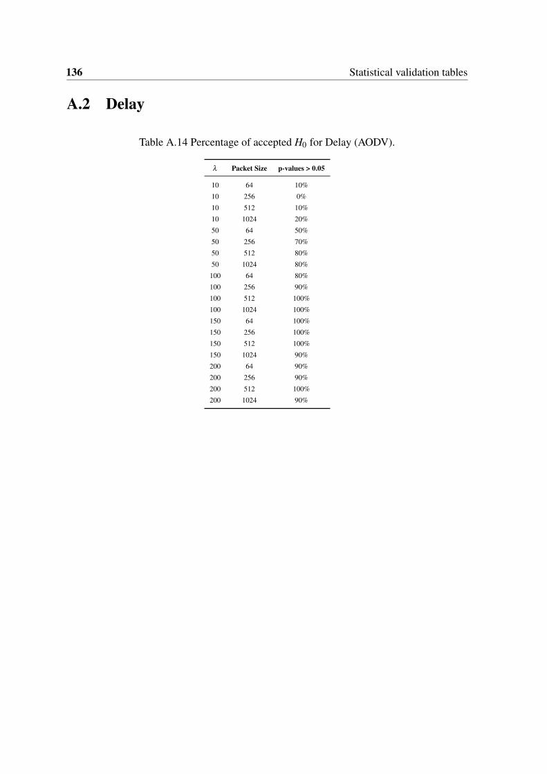
136 Statistical validation tables
A.2 Delay
Table A.14 Percentage of accepted H0 for Delay (AODV).
λ Packet Size p-values > 0.05
10 64 10%
10 256 0%
10 512 10%
10 1024 20%
50 64 50%
50 256 70%
50 512 80%
50 1024 80%
100 64 80%
100 256 90%
100 512 100%
100 1024 100%
150 64 100%
150 256 100%
150 512 100%
150 1024 90%
200 64 90%
200 256 90%
200 512 100%
200 1024 90%

A.2 Delay 137
Table A.15 Delay statistics for λ = 10 and packet size of 256 bytes.
Nodes Analytical Simulated CI p-value
2 1.46e-04 3.11e-04 (3.10e-04,3.11e-04) 1.00e+00
4 1.48e-04 4.49e-04 (3.80e-04,5.18e-04) 9.94e-01
6 1.51e-04 5.61e-04 (3.28e-04,7.94e-04) 9.66e-01
8 1.58e-04 9.17e-04 (5.89e-04,1.25e-03) 9.80e-01
10 1.66e-04 1.29e-03 (9.59e-04,1.63e-03) 9.90e-01
12 1.73e-04 1.67e-03 (1.45e-03,1.90e-03) 9.98e-01
14 1.88e-04 2.52e-03 (1.70e-03,3.33e-03) 9.87e-01
16 1.98e-04 2.18e-03 (2.07e-03,2.29e-03) 1.00e+00
18 2.20e-04 2.56e-03 (2.17e-03,2.95e-03) 9.97e-01
20 2.36e-04 3.48e-03 (1.54e-03,5.41e-03) 9.65e-01
Table A.16 Delay statistics for λ = 10 and packet size of 512 bytes.
Nodes Analytical Simulated CI p-value
2 1.50e-04 4.90e-04 (4.90e-04,4.91e-04) 1.00e+00
4 1.54e-04 7.44e-04 (6.43e-04,8.47e-04) 9.97e-01
6 1.58e-04 1.03e-03 (5.67e-04,1.50e-03) 9.70e-01
8 1.73e-04 1.68e-03 (1.17e-03,2.20e-03) 9.87e-01
10 1.87e-04 3.35e-03 (1.75e-03,4.94e-03) 9.73e-01
12 2.03e-04 3.94e-03 (2.57e-03,5.30e-03) 9.85e-01
14 2.38e-04 5.61e-03 (4.10e-03,7.11e-03) 9.91e-01
16 2.67e-04 6.24e-03 (5.10e-03,7.37e-03) 9.96e-01
18 3.40e-04 6.08e-03 (4.40e-03,7.78e-03) 9.91e-01
20 4.21e-04 1.07e-02 (1.77e-03,1.97e-02) 9.31e-01
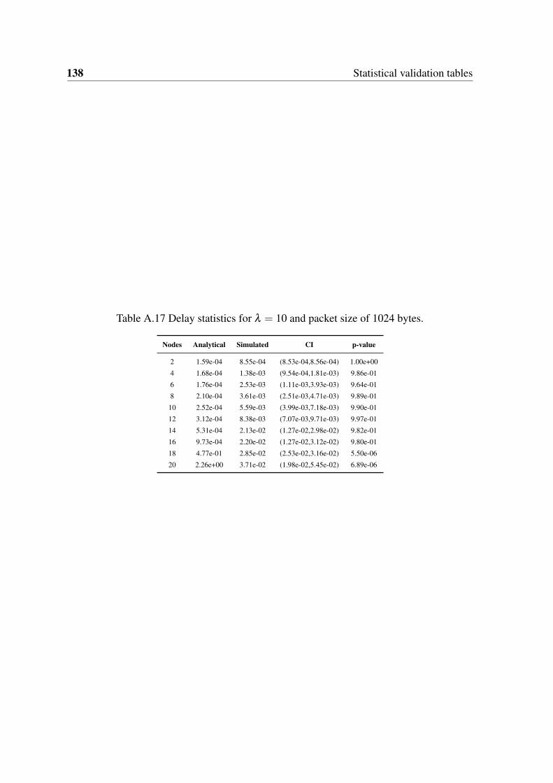
138 Statistical validation tables
Table A.17 Delay statistics for λ = 10 and packet size of 1024 bytes.
Nodes Analytical Simulated CI p-value
2 1.59e-04 8.55e-04 (8.53e-04,8.56e-04) 1.00e+00
4 1.68e-04 1.38e-03 (9.54e-04,1.81e-03) 9.86e-01
6 1.76e-04 2.53e-03 (1.11e-03,3.93e-03) 9.64e-01
8 2.10e-04 3.61e-03 (2.51e-03,4.71e-03) 9.89e-01
10 2.52e-04 5.59e-03 (3.99e-03,7.18e-03) 9.90e-01
12 3.12e-04 8.38e-03 (7.07e-03,9.71e-03) 9.97e-01
14 5.31e-04 2.13e-02 (1.27e-02,2.98e-02) 9.82e-01
16 9.73e-04 2.20e-02 (1.27e-02,3.12e-02) 9.80e-01
18 4.77e-01 2.85e-02 (2.53e-02,3.16e-02) 5.50e-06
20 2.26e+00 3.71e-02 (1.98e-02,5.45e-02) 6.89e-06
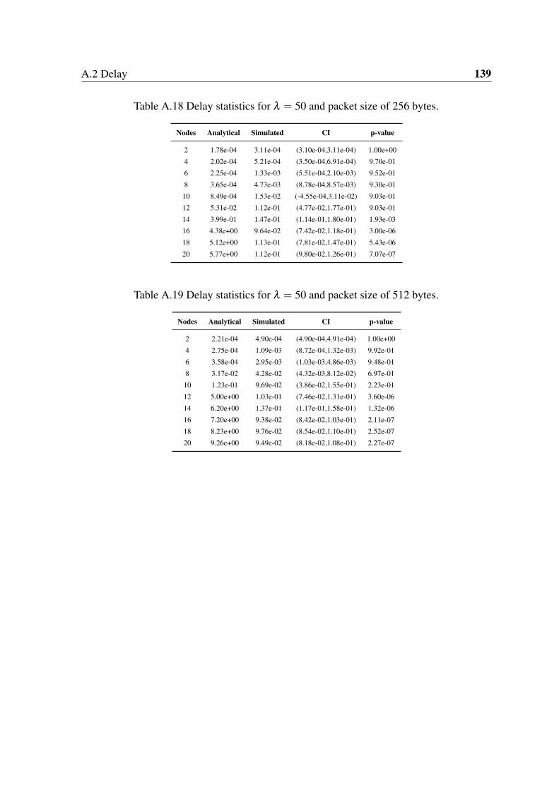
A.2 Delay 139
Table A.18 Delay statistics for λ = 50 and packet size of 256 bytes.
Nodes Analytical Simulated CI p-value
2 1.78e-04 3.11e-04 (3.10e-04,3.11e-04) 1.00e+00
4 2.02e-04 5.21e-04 (3.50e-04,6.91e-04) 9.70e-01
6 2.25e-04 1.33e-03 (5.51e-04,2.10e-03) 9.52e-01
8 3.65e-04 4.73e-03 (8.78e-04,8.57e-03) 9.30e-01
10 8.49e-04 1.53e-02 (-4.55e-04,3.11e-02) 9.03e-01
12 5.31e-02 1.12e-01 (4.77e-02,1.77e-01) 9.03e-01
14 3.99e-01 1.47e-01 (1.14e-01,1.80e-01) 1.93e-03
16 4.38e+00 9.64e-02 (7.42e-02,1.18e-01) 3.00e-06
18 5.12e+00 1.13e-01 (7.81e-02,1.47e-01) 5.43e-06
20 5.77e+00 1.12e-01 (9.80e-02,1.26e-01) 7.07e-07
Table A.19 Delay statistics for λ = 50 and packet size of 512 bytes.
Nodes Analytical Simulated CI p-value
2 2.21e-04 4.90e-04 (4.90e-04,4.91e-04) 1.00e+00
4 2.75e-04 1.09e-03 (8.72e-04,1.32e-03) 9.92e-01
6 3.58e-04 2.95e-03 (1.03e-03,4.86e-03) 9.48e-01
8 3.17e-02 4.28e-02 (4.32e-03,8.12e-02) 6.97e-01
10 1.23e-01 9.69e-02 (3.86e-02,1.55e-01) 2.23e-01
12 5.00e+00 1.03e-01 (7.46e-02,1.31e-01) 3.60e-06
14 6.20e+00 1.37e-01 (1.17e-01,1.58e-01) 1.32e-06
16 7.20e+00 9.38e-02 (8.42e-02,1.03e-01) 2.11e-07
18 8.23e+00 9.76e-02 (8.54e-02,1.10e-01) 2.52e-07
20 9.26e+00 9.49e-02 (8.18e-02,1.08e-01) 2.27e-07

140 Statistical validation tables
Table A.20 Delay statistics for λ = 50 and packet size of 1024 bytes.
Nodes Analytical Simulated CI p-value
2 3.94e-04 8.56e-04 (8.56e-04,8.57e-04) 1.00e+00
4 1.03e-03 3.22e-03 (2.66e-03,3.77e-03) 9.93e-01
6 3.30e-02 7.66e-02 (1.47e-02,1.39e-01) 8.61e-01
8 2.73e+00 8.70e-02 (4.55e-02,1.29e-01) 2.79e-05
10 7.63e+00 1.29e-01 (9.48e-02,1.64e-01) 2.47e-06
12 9.38e+00 8.70e-02 (6.00e-02,1.14e-01) 9.50e-07
14 1.12e+01 1.05e-01 (6.84e-02,1.41e-01) 1.21e-06
16 1.30e+01 9.25e-02 (6.34e-02,1.22e-01) 5.90e-07
18 1.48e+01 9.98e-02 (5.15e-02,1.47e-01) 1.18e-06
20 1.67e+01 8.08e-02 (5.43e-02,1.07e-01) 2.86e-07
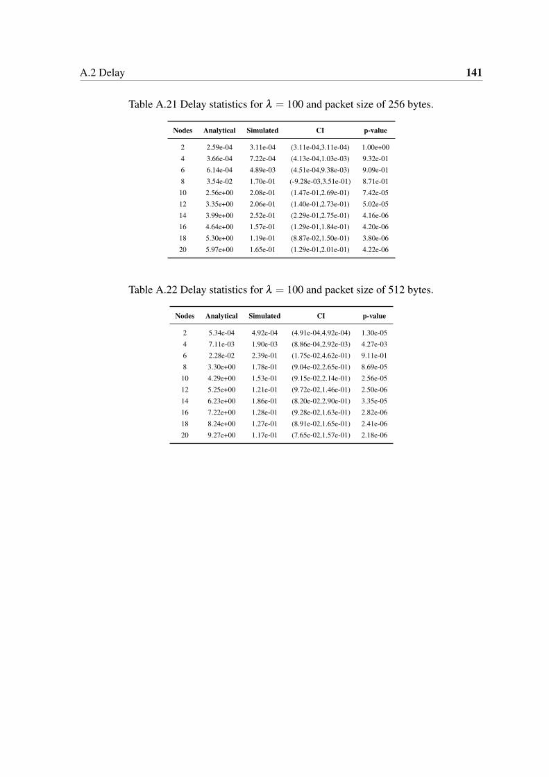
A.2 Delay 141
Table A.21 Delay statistics for λ = 100 and packet size of 256 bytes.
Nodes Analytical Simulated CI p-value
2 2.59e-04 3.11e-04 (3.11e-04,3.11e-04) 1.00e+00
4 3.66e-04 7.22e-04 (4.13e-04,1.03e-03) 9.32e-01
6 6.14e-04 4.89e-03 (4.51e-04,9.38e-03) 9.09e-01
8 3.54e-02 1.70e-01 (-9.28e-03,3.51e-01) 8.71e-01
10 2.56e+00 2.08e-01 (1.47e-01,2.69e-01) 7.42e-05
12 3.35e+00 2.06e-01 (1.40e-01,2.73e-01) 5.02e-05
14 3.99e+00 2.52e-01 (2.29e-01,2.75e-01) 4.16e-06
16 4.64e+00 1.57e-01 (1.29e-01,1.84e-01) 4.20e-06
18 5.30e+00 1.19e-01 (8.87e-02,1.50e-01) 3.80e-06
20 5.97e+00 1.65e-01 (1.29e-01,2.01e-01) 4.22e-06
Table A.22 Delay statistics for λ = 100 and packet size of 512 bytes.
Nodes Analytical Simulated CI p-value
2 5.34e-04 4.92e-04 (4.91e-04,4.92e-04) 1.30e-05
4 7.11e-03 1.90e-03 (8.86e-04,2.92e-03) 4.27e-03
6 2.28e-02 2.39e-01 (1.75e-02,4.62e-01) 9.11e-01
8 3.30e+00 1.78e-01 (9.04e-02,2.65e-01) 8.69e-05
10 4.29e+00 1.53e-01 (9.15e-02,2.14e-01) 2.56e-05
12 5.25e+00 1.21e-01 (9.72e-02,1.46e-01) 2.50e-06
14 6.23e+00 1.86e-01 (8.20e-02,2.90e-01) 3.35e-05
16 7.22e+00 1.28e-01 (9.28e-02,1.63e-01) 2.82e-06
18 8.24e+00 1.27e-01 (8.91e-02,1.65e-01) 2.41e-06
20 9.27e+00 1.17e-01 (7.65e-02,1.57e-01) 2.18e-06
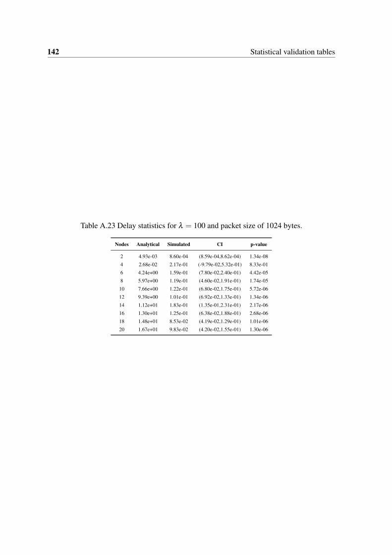
142 Statistical validation tables
Table A.23 Delay statistics for λ = 100 and packet size of 1024 bytes.
Nodes Analytical Simulated CI p-value
2 4.93e-03 8.60e-04 (8.59e-04,8.62e-04) 1.34e-08
4 2.68e-02 2.17e-01 (-9.79e-02,5.32e-01) 8.33e-01
6 4.24e+00 1.59e-01 (7.80e-02,2.40e-01) 4.42e-05
8 5.97e+00 1.19e-01 (4.60e-02,1.91e-01) 1.74e-05
10 7.66e+00 1.22e-01 (6.80e-02,1.75e-01) 5.72e-06
12 9.39e+00 1.01e-01 (6.92e-02,1.33e-01) 1.34e-06
14 1.12e+01 1.83e-01 (1.35e-01,2.31e-01) 2.17e-06
16 1.30e+01 1.25e-01 (6.38e-02,1.88e-01) 2.68e-06
18 1.48e+01 8.53e-02 (4.19e-02,1.29e-01) 1.01e-06
20 1.67e+01 9.83e-02 (4.20e-02,1.55e-01) 1.30e-06
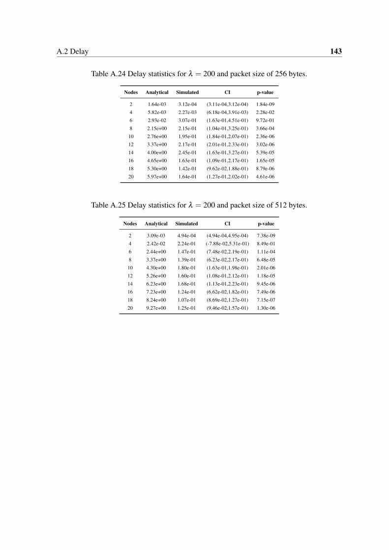
A.2 Delay 143
Table A.24 Delay statistics for λ = 200 and packet size of 256 bytes.
Nodes Analytical Simulated CI p-value
2 1.64e-03 3.12e-04 (3.11e-04,3.12e-04) 1.84e-09
4 5.82e-03 2.27e-03 (6.18e-04,3.91e-03) 2.28e-02
6 2.93e-02 3.07e-01 (1.63e-01,4.51e-01) 9.72e-01
8 2.15e+00 2.15e-01 (1.04e-01,3.25e-01) 3.66e-04
10 2.76e+00 1.95e-01 (1.84e-01,2.07e-01) 2.36e-06
12 3.37e+00 2.17e-01 (2.01e-01,2.33e-01) 3.02e-06
14 4.00e+00 2.45e-01 (1.63e-01,3.27e-01) 5.39e-05
16 4.65e+00 1.63e-01 (1.09e-01,2.17e-01) 1.65e-05
18 5.30e+00 1.42e-01 (9.62e-02,1.88e-01) 8.79e-06
20 5.97e+00 1.64e-01 (1.27e-01,2.02e-01) 4.61e-06
Table A.25 Delay statistics for λ = 200 and packet size of 512 bytes.
Nodes Analytical Simulated CI p-value
2 3.09e-03 4.94e-04 (4.94e-04,4.95e-04) 7.38e-09
4 2.42e-02 2.24e-01 (-7.88e-02,5.31e-01) 8.49e-01
6 2.44e+00 1.47e-01 (7.48e-02,2.19e-01) 1.11e-04
8 3.37e+00 1.39e-01 (6.23e-02,2.17e-01) 6.48e-05
10 4.30e+00 1.80e-01 (1.63e-01,1.98e-01) 2.01e-06
12 5.26e+00 1.60e-01 (1.08e-01,2.12e-01) 1.18e-05
14 6.23e+00 1.68e-01 (1.13e-01,2.23e-01) 9.45e-06
16 7.23e+00 1.24e-01 (6.62e-02,1.82e-01) 7.49e-06
18 8.24e+00 1.07e-01 (8.69e-02,1.27e-01) 7.15e-07
20 9.27e+00 1.25e-01 (9.46e-02,1.57e-01) 1.30e-06

144 Statistical validation tables
Table A.26 Delay statistics for λ = 200 and packet size of 1024 bytes.
Nodes Analytical Simulated CI p-value
2 0.00e+00 8.73e-04 (8.72e-04,8.75e-04) 1.00e+00
4 2.76e+00 1.65e-01 (1.12e-01,2.17e-01) 4.53e-05
6 4.28e+00 1.55e-01 (6.35e-02,2.45e-01) 5.47e-05
8 5.87e+00 1.18e-01 (3.67e-02,1.99e-01) 2.29e-05
10 7.50e+00 1.37e-01 (4.02e-02,2.35e-01) 1.96e-05
12 9.18e+00 1.10e-01 (4.44e-02,1.77e-01) 6.10e-06
14 1.09e+01 1.68e-01 (8.98e-02,2.47e-01) 6.06e-06
16 1.26e+01 2.02e-01 (4.46e-02,3.58e-01) 1.78e-05
18 1.44e+01 1.39e-01 (1.82e-02,2.61e-01) 8.20e-06
20 1.62e+01 8.69e-02 (2.84e-02,1.45e-01) 1.44e-06
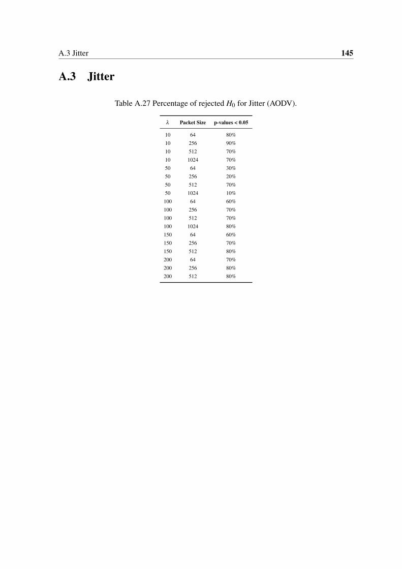
A.3 Jitter 145
A.3 Jitter
Table A.27 Percentage of rejected H0 for Jitter (AODV).
λ Packet Size p-values < 0.05
10 64 80%
10 256 90%
10 512 70%
10 1024 70%
50 64 30%
50 256 20%
50 512 70%
50 1024 10%
100 64 60%
100 256 70%
100 512 70%
100 1024 80%
150 64 60%
150 256 70%
150 512 80%
200 64 70%
200 256 80%
200 512 80%
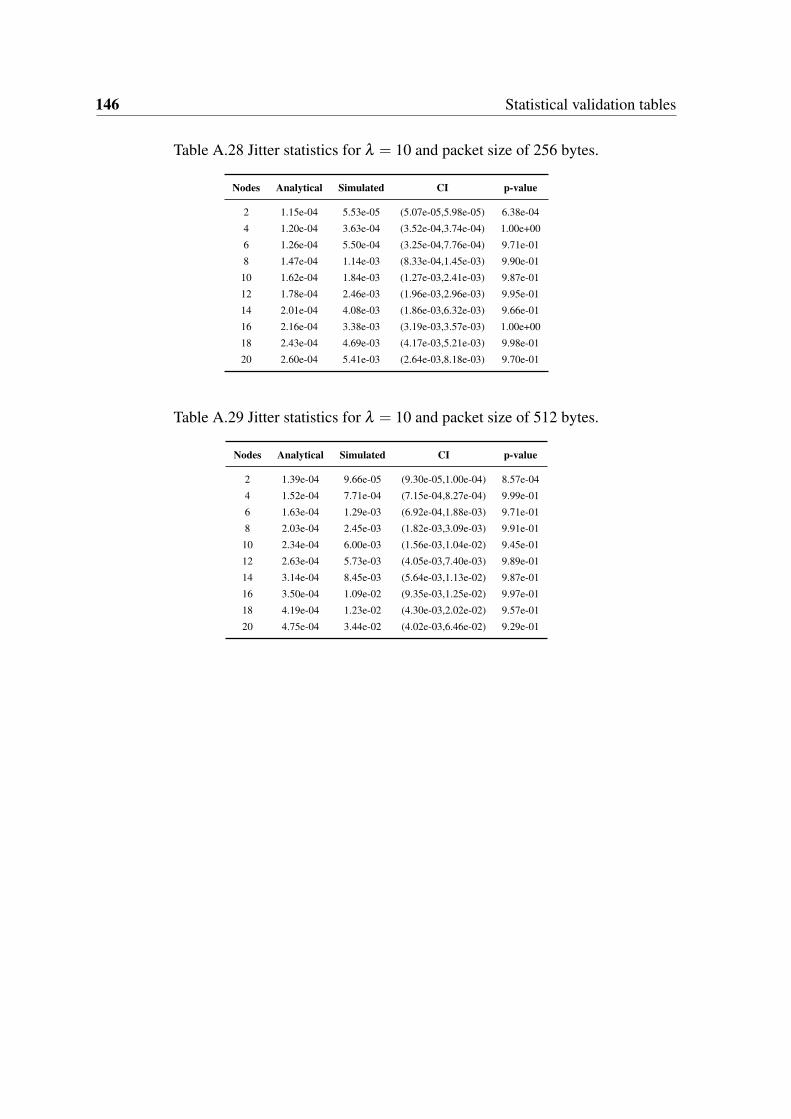
146 Statistical validation tables
Table A.28 Jitter statistics for λ = 10 and packet size of 256 bytes.
Nodes Analytical Simulated CI p-value
2 1.15e-04 5.53e-05 (5.07e-05,5.98e-05) 6.38e-04
4 1.20e-04 3.63e-04 (3.52e-04,3.74e-04) 1.00e+00
6 1.26e-04 5.50e-04 (3.25e-04,7.76e-04) 9.71e-01
8 1.47e-04 1.14e-03 (8.33e-04,1.45e-03) 9.90e-01
10 1.62e-04 1.84e-03 (1.27e-03,2.41e-03) 9.87e-01
12 1.78e-04 2.46e-03 (1.96e-03,2.96e-03) 9.95e-01
14 2.01e-04 4.08e-03 (1.86e-03,6.32e-03) 9.66e-01
16 2.16e-04 3.38e-03 (3.19e-03,3.57e-03) 1.00e+00
18 2.43e-04 4.69e-03 (4.17e-03,5.21e-03) 9.98e-01
20 2.60e-04 5.41e-03 (2.64e-03,8.18e-03) 9.70e-01
Table A.29 Jitter statistics for λ = 10 and packet size of 512 bytes.
Nodes Analytical Simulated CI p-value
2 1.39e-04 9.66e-05 (9.30e-05,1.00e-04) 8.57e-04
4 1.52e-04 7.71e-04 (7.15e-04,8.27e-04) 9.99e-01
6 1.63e-04 1.29e-03 (6.92e-04,1.88e-03) 9.71e-01
8 2.03e-04 2.45e-03 (1.82e-03,3.09e-03) 9.91e-01
10 2.34e-04 6.00e-03 (1.56e-03,1.04e-02) 9.45e-01
12 2.63e-04 5.73e-03 (4.05e-03,7.40e-03) 9.89e-01
14 3.14e-04 8.45e-03 (5.64e-03,1.13e-02) 9.87e-01
16 3.50e-04 1.09e-02 (9.35e-03,1.25e-02) 9.97e-01
18 4.19e-04 1.23e-02 (4.30e-03,2.02e-02) 9.57e-01
20 4.75e-04 3.44e-02 (4.02e-03,6.46e-02) 9.29e-01

A.3 Jitter 147
Table A.30 Jitter statistics for λ = 10 and packet size of 1024 bytes.
Nodes Analytical Simulated CI p-value
2 2.04e-04 2.04e-04 (1.93e-04,2.15e-04) 5.33e-01
4 2.33e-04 1.63e-03 (1.02e-03,2.25e-03) 9.80e-01
6 2.60e-04 3.61e-03 (1.71e-03,5.52e-03) 9.67e-01
8 3.49e-04 5.17e-03 (3.97e-03,6.37e-03) 9.93e-01
10 4.29e-04 7.63e-03 (6.06e-03,9.19e-03) 9.95e-01
12 5.15e-04 1.49e-02 (9.97e-03,1.99e-02) 9.87e-01
14 7.13e-04 6.14e-02 (4.97e-02,7.33e-02) 9.96e-01
16 9.99e-04 5.90e-02 (3.21e-02,8.58e-02) 9.78e-01
18 6.44e-01 7.23e-02 (6.67e-02,7.79e-02) 1.10e-05
20 1.70e+00 8.88e-02 (5.84e-02,1.19e-01) 3.93e-05

148 Statistical validation tables
Table A.31 Jitter statistics for λ = 50 and packet size of 256 bytes.
Nodes Analytical Simulated CI p-value
2 2.25e-04 5.48e-05 (5.37e-05,5.59e-05) 4.71e-06
4 2.52e-04 6.99e-04 (4.68e-04,9.29e-04) 9.73e-01
6 2.78e-04 3.16e-03 (1.06e-03,5.27e-03) 9.49e-01
8 4.10e-04 7.95e-03 (2.45e-03,1.35e-02) 9.48e-01
10 7.94e-04 5.60e-02 (3.61e-03,1.08e-01) 9.22e-01
12 8.94e-02 2.62e-01 (1.64e-01,3.61e-01) 9.67e-01
14 3.10e-01 3.28e-01 (2.88e-01,3.68e-01) 7.83e-01
16 3.10e-01 2.44e-01 (2.10e-01,2.77e-01) 2.62e-02
18 3.10e-01 2.82e-01 (2.21e-01,3.44e-01) 2.26e-01
20 3.10e-01 2.84e-01 (2.70e-01,2.97e-01) 2.90e-02
Table A.32 Jitter statistics for λ = 50 and packet size of 512 bytes.
Nodes Analytical Simulated CI p-value
2 3.17e-04 9.98e-05 (9.74e-05,1.02e-04) 1.41e-05
4 3.83e-04 1.85e-03 (1.77e-03,1.93e-03) 1.00e+00
6 4.55e-04 4.84e-03 (2.13e-03,7.53e-03) 9.62e-01
8 6.07e-02 1.23e-01 (5.23e-02,1.93e-01) 8.99e-01
10 1.74e-01 2.59e-01 (1.41e-01,3.78e-01) 8.66e-01
12 1.74e-01 3.06e-01 (2.32e-01,3.78e-01) 9.69e-01
14 1.74e-01 3.90e-01 (3.43e-01,4.37e-01) 9.95e-01
16 1.74e-01 3.06e-01 (2.69e-01,3.43e-01) 9.91e-01
18 1.74e-01 2.89e-01 (2.70e-01,3.08e-01) 9.97e-01
20 1.74e-01 3.10e-01 (2.99e-01,3.21e-01) 9.99e-01

A.3 Jitter 149
Table A.33 Jitter statistics for λ = 50 and packet size of 1024 bytes.
Nodes Analytical Simulated CI p-value
2 6.23e-04 2.12e-04 (2.11e-04,2.13e-04) 5.53e-07
4 1.07e-03 5.77e-03 (5.66e-03,5.88e-03) 1.00e+00
6 6.08e-02 2.23e-01 (7.01e-02,3.74e-01) 9.24e-01
8 1.54e+00 3.28e-01 (2.26e-01,4.29e-01) 8.16e-04
10 1.54e+00 5.08e-01 (3.81e-01,6.35e-01) 1.68e-03
12 1.54e+00 3.94e-01 (3.25e-01,4.63e-01) 4.11e-04
14 1.54e+00 4.08e-01 (3.50e-01,4.67e-01) 3.06e-04
16 1.54e+00 4.09e-01 (3.35e-01,4.83e-01) 4.94e-04
18 1.54e+00 3.80e-01 (3.09e-01,4.50e-01) 4.23e-04
20 1.54e+00 3.87e-01 (3.61e-01,4.14e-01) 6.12e-05

150 Statistical validation tables
Table A.34 Jitter statistics for λ = 100 and packet size of 256 bytes.
Nodes Analytical Simulated CI p-value
2 3.59e-04 5.81e-05 (5.59e-05,6.03e-05) 5.94e-06
4 4.44e-04 1.25e-03 (7.19e-04,1.77e-03) 9.58e-01
6 6.32e-04 1.12e-02 (5.49e-04,2.19e-02) 9.13e-01
8 5.80e-02 3.70e-01 (6.49e-02,6.73e-01) 9.20e-01
10 5.80e-02 6.30e-01 (5.53e-01,7.06e-01) 9.98e-01
12 5.80e-02 5.51e-01 (3.84e-01,7.21e-01) 9.87e-01
14 5.80e-02 6.48e-01 (5.74e-01,7.22e-01) 9.98e-01
16 5.80e-02 4.80e-01 (4.18e-01,5.42e-01) 9.98e-01
18 5.80e-02 3.82e-01 (3.52e-01,4.13e-01) 9.99e-01
20 5.80e-02 5.00e-01 (3.82e-01,6.17e-01) 9.92e-01
Table A.35 Jitter statistics for λ = 100 and packet size of 512 bytes.
Nodes Analytical Simulated CI p-value
2 6.29e-04 1.08e-04 (1.06e-04,1.10e-04) 1.67e-06
4 2.20e-03 3.51e-03 (1.84e-03,5.17e-03) 8.78e-01
6 4.06e-02 5.46e-01 (1.44e-01,9.54e-01) 9.41e-01
8 4.06e-02 5.43e-01 (4.14e-01,6.73e-01) 9.93e-01
10 4.06e-02 6.31e-01 (5.10e-01,7.53e-01) 9.95e-01
12 4.06e-02 5.36e-01 (4.87e-01,5.86e-01) 9.99e-01
14 4.06e-02 6.34e-01 (4.18e-01,8.52e-01) 9.85e-01
16 4.06e-02 4.87e-01 (4.15e-01,5.59e-01) 9.97e-01
18 4.06e-02 4.78e-01 (3.98e-01,5.56e-01) 9.96e-01
20 4.06e-02 4.41e-01 (4.04e-01,4.76e-01) 9.99e-01
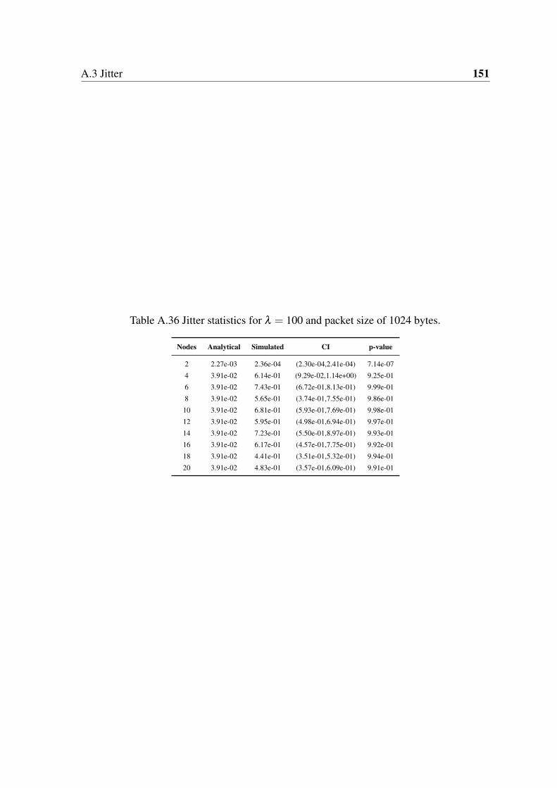
A.3 Jitter 151
Table A.36 Jitter statistics for λ = 100 and packet size of 1024 bytes.
Nodes Analytical Simulated CI p-value
2 2.27e-03 2.36e-04 (2.30e-04,2.41e-04) 7.14e-07
4 3.91e-02 6.14e-01 (9.29e-02,1.14e+00) 9.25e-01
6 3.91e-02 7.43e-01 (6.72e-01,8.13e-01) 9.99e-01
8 3.91e-02 5.65e-01 (3.74e-01,7.55e-01) 9.86e-01
10 3.91e-02 6.81e-01 (5.93e-01,7.69e-01) 9.98e-01
12 3.91e-02 5.95e-01 (4.98e-01,6.94e-01) 9.97e-01
14 3.91e-02 7.23e-01 (5.50e-01,8.97e-01) 9.93e-01
16 3.91e-02 6.17e-01 (4.57e-01,7.75e-01) 9.92e-01
18 3.91e-02 4.41e-01 (3.51e-01,5.32e-01) 9.94e-01
20 3.91e-02 4.83e-01 (3.57e-01,6.09e-01) 9.91e-01
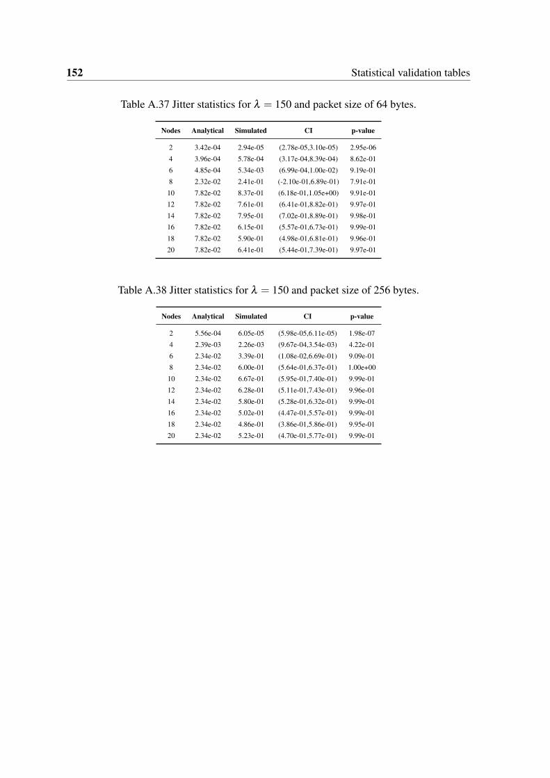
152 Statistical validation tables
Table A.37 Jitter statistics for λ = 150 and packet size of 64 bytes.
Nodes Analytical Simulated CI p-value
2 3.42e-04 2.94e-05 (2.78e-05,3.10e-05) 2.95e-06
4 3.96e-04 5.78e-04 (3.17e-04,8.39e-04) 8.62e-01
6 4.85e-04 5.34e-03 (6.99e-04,1.00e-02) 9.19e-01
8 2.32e-02 2.41e-01 (-2.10e-01,6.89e-01) 7.91e-01
10 7.82e-02 8.37e-01 (6.18e-01,1.05e+00) 9.91e-01
12 7.82e-02 7.61e-01 (6.41e-01,8.82e-01) 9.97e-01
14 7.82e-02 7.95e-01 (7.02e-01,8.89e-01) 9.98e-01
16 7.82e-02 6.15e-01 (5.57e-01,6.73e-01) 9.99e-01
18 7.82e-02 5.90e-01 (4.98e-01,6.81e-01) 9.96e-01
20 7.82e-02 6.41e-01 (5.44e-01,7.39e-01) 9.97e-01
Table A.38 Jitter statistics for λ = 150 and packet size of 256 bytes.
Nodes Analytical Simulated CI p-value
2 5.56e-04 6.05e-05 (5.98e-05,6.11e-05) 1.98e-07
4 2.39e-03 2.26e-03 (9.67e-04,3.54e-03) 4.22e-01
6 2.34e-02 3.39e-01 (1.08e-02,6.69e-01) 9.09e-01
8 2.34e-02 6.00e-01 (5.64e-01,6.37e-01) 1.00e+00
10 2.34e-02 6.67e-01 (5.95e-01,7.40e-01) 9.99e-01
12 2.34e-02 6.28e-01 (5.11e-01,7.43e-01) 9.96e-01
14 2.34e-02 5.80e-01 (5.28e-01,6.32e-01) 9.99e-01
16 2.34e-02 5.02e-01 (4.47e-01,5.57e-01) 9.99e-01
18 2.34e-02 4.86e-01 (3.86e-01,5.86e-01) 9.95e-01
20 2.34e-02 5.23e-01 (4.70e-01,5.77e-01) 9.99e-01

A.3 Jitter 153
Table A.39 Jitter statistics for λ = 150 and packet size of 512 bytes.
Nodes Analytical Simulated CI p-value
2 1.99e-03 1.14e-04 (1.14e-04,1.15e-04) 1.36e-09
4 1.81e-02 1.25e-02 (1.19e-02,1.30e-02) 1.12e-03
6 1.68e-01 7.11e-01 (5.88e-01,8.33e-01) 9.94e-01
8 1.68e-01 5.83e-01 (4.46e-01,7.20e-01) 9.88e-01
10 1.68e-01 6.77e-01 (5.88e-01,7.66e-01) 9.97e-01
12 1.68e-01 6.03e-01 (5.19e-01,6.88e-01) 9.96e-01
14 1.68e-01 6.51e-01 (6.09e-01,6.93e-01) 9.99e-01
16 1.68e-01 5.60e-01 (5.35e-01,5.84e-01) 1.00e+00
18 1.68e-01 4.49e-01 (3.67e-01,5.31e-01) 9.91e-01
20 1.68e-01 5.31e-01 (4.40e-01,6.21e-01) 9.93e-01
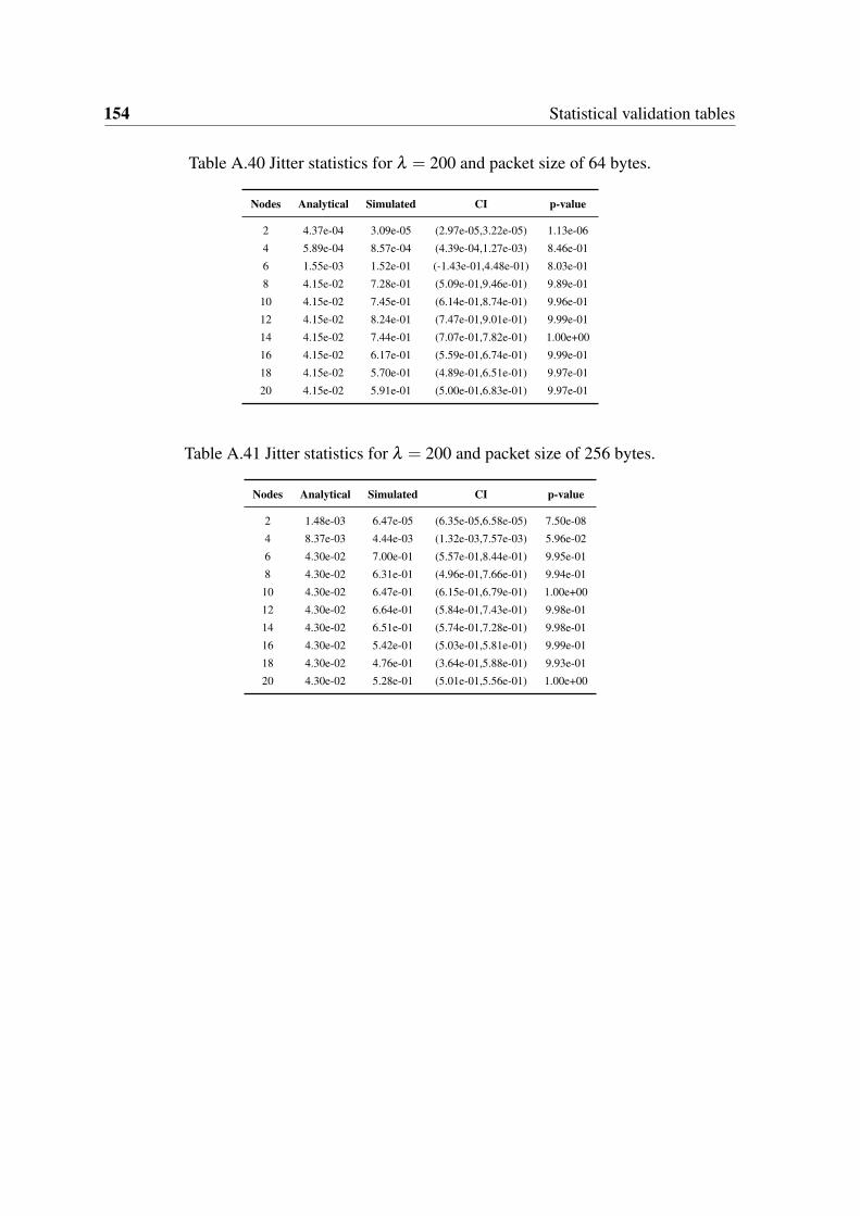
154 Statistical validation tables
Table A.40 Jitter statistics for λ = 200 and packet size of 64 bytes.
Nodes Analytical Simulated CI p-value
2 4.37e-04 3.09e-05 (2.97e-05,3.22e-05) 1.13e-06
4 5.89e-04 8.57e-04 (4.39e-04,1.27e-03) 8.46e-01
6 1.55e-03 1.52e-01 (-1.43e-01,4.48e-01) 8.03e-01
8 4.15e-02 7.28e-01 (5.09e-01,9.46e-01) 9.89e-01
10 4.15e-02 7.45e-01 (6.14e-01,8.74e-01) 9.96e-01
12 4.15e-02 8.24e-01 (7.47e-01,9.01e-01) 9.99e-01
14 4.15e-02 7.44e-01 (7.07e-01,7.82e-01) 1.00e+00
16 4.15e-02 6.17e-01 (5.59e-01,6.74e-01) 9.99e-01
18 4.15e-02 5.70e-01 (4.89e-01,6.51e-01) 9.97e-01
20 4.15e-02 5.91e-01 (5.00e-01,6.83e-01) 9.97e-01
Table A.41 Jitter statistics for λ = 200 and packet size of 256 bytes.
Nodes Analytical Simulated CI p-value
2 1.48e-03 6.47e-05 (6.35e-05,6.58e-05) 7.50e-08
4 8.37e-03 4.44e-03 (1.32e-03,7.57e-03) 5.96e-02
6 4.30e-02 7.00e-01 (5.57e-01,8.44e-01) 9.95e-01
8 4.30e-02 6.31e-01 (4.96e-01,7.66e-01) 9.94e-01
10 4.30e-02 6.47e-01 (6.15e-01,6.79e-01) 1.00e+00
12 4.30e-02 6.64e-01 (5.84e-01,7.43e-01) 9.98e-01
14 4.30e-02 6.51e-01 (5.74e-01,7.28e-01) 9.98e-01
16 4.30e-02 5.42e-01 (5.03e-01,5.81e-01) 9.99e-01
18 4.30e-02 4.76e-01 (3.64e-01,5.88e-01) 9.93e-01
20 4.30e-02 5.28e-01 (5.01e-01,5.56e-01) 1.00e+00
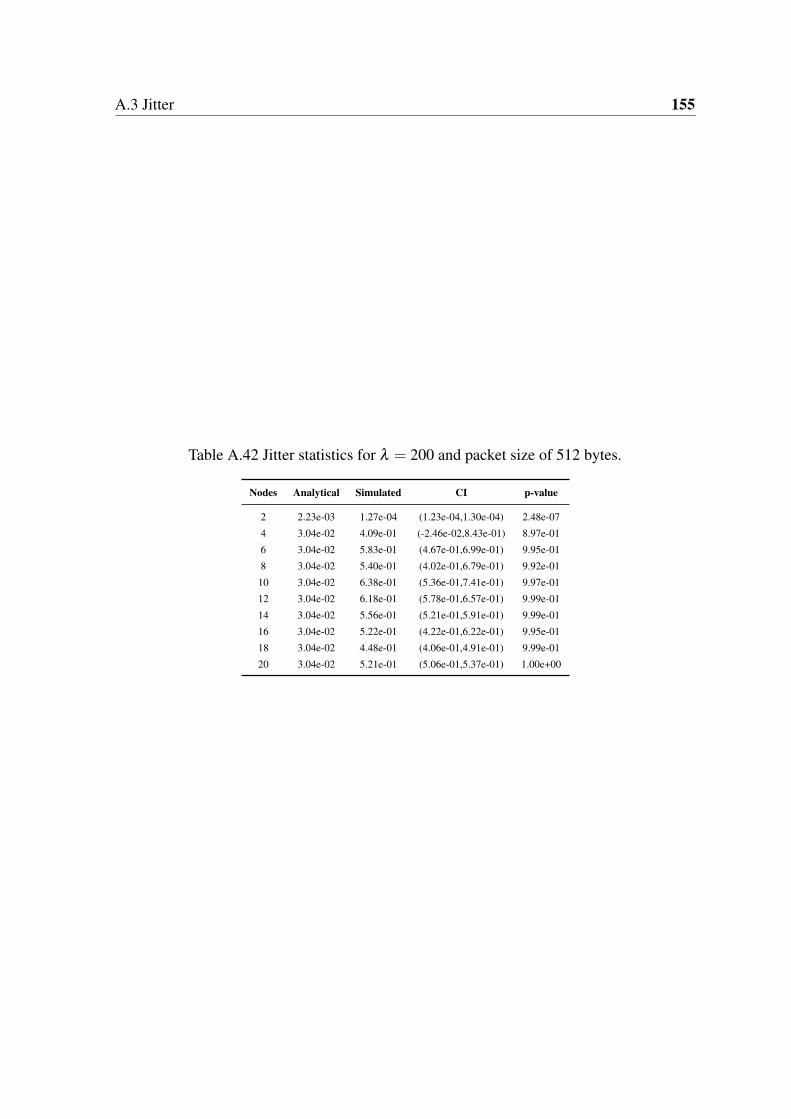
A.3 Jitter 155
Table A.42 Jitter statistics for λ = 200 and packet size of 512 bytes.
Nodes Analytical Simulated CI p-value
2 2.23e-03 1.27e-04 (1.23e-04,1.30e-04) 2.48e-07
4 3.04e-02 4.09e-01 (-2.46e-02,8.43e-01) 8.97e-01
6 3.04e-02 5.83e-01 (4.67e-01,6.99e-01) 9.95e-01
8 3.04e-02 5.40e-01 (4.02e-01,6.79e-01) 9.92e-01
10 3.04e-02 6.38e-01 (5.36e-01,7.41e-01) 9.97e-01
12 3.04e-02 6.18e-01 (5.78e-01,6.57e-01) 9.99e-01
14 3.04e-02 5.56e-01 (5.21e-01,5.91e-01) 9.99e-01
16 3.04e-02 5.22e-01 (4.22e-01,6.22e-01) 9.95e-01
18 3.04e-02 4.48e-01 (4.06e-01,4.91e-01) 9.99e-01
20 3.04e-02 5.21e-01 (5.06e-01,5.37e-01) 1.00e+00
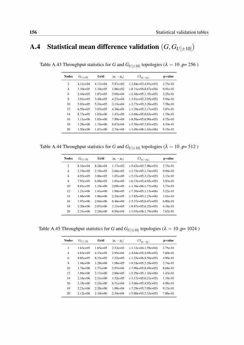
156 Statistical validation tables
A.4 Statistical mean difference validation (G,GU [±10])
Table A.43 Throughput statistics for G and GU [±10] topologies (λ = 10 ,p= 256 )
Nodes GU [±20] Grid |µr−µg| CI|µr−µg | p-value
2 4.11e+04 4.17e+04 5.87e+02 (-2.84e+03,4.01e+03) 2.75e-01
4 1.10e+05 1.10e+05 1.86e+02 (-8.71e+04,8.67e+04) 9.91e-01
6 2.44e+05 1.87e+05 5.69e+04 (-2.48e+05,1.35e+05) 2.25e-01
8 3.91e+05 3.49e+05 4.27e+04 (-3.91e+05,3.05e+05) 5.94e-01
10 5.03e+05 5.24e+05 2.13e+04 (-2.77e+05,3.20e+05) 7.58e-01
12 6.59e+05 7.03e+05 4.38e+04 (-1.29e+05,2.17e+05) 3.07e-01
14 8.73e+05 1.02e+06 1.47e+05 (-5.68e+05,8.63e+05) 1.79e-01
16 1.11e+06 1.03e+06 7.99e+04 (-8.50e+05,6.90e+05) 4.75e-01
18 1.28e+06 1.19e+06 8.67e+04 (-5.56e+05,3.83e+05) 4.10e-01
20 1.50e+06 1.47e+06 2.74e+04 (-1.49e+06,1.43e+06) 9.15e-01
Table A.44 Throughput statistics for G and GU [±10] topologies (λ = 10 ,p= 512 )
Nodes GU [±20] Grid |µr−µg| CI|µr−µg | p-value
2 8.16e+04 8.28e+04 1.17e+03 (-5.63e+03,7.96e+03) 2.75e-01
4 2.19e+05 2.19e+05 2.66e+02 (-1.73e+05,1.74e+05) 9.94e-01
6 4.93e+05 3.86e+05 1.07e+05 (-5.37e+05,3.23e+05) 3.13e-01
8 7.93e+05 6.88e+05 1.05e+05 (-6.15e+05,4.05e+05) 3.93e-01
10 9.81e+05 1.19e+06 2.09e+05 (-1.36e+06,1.77e+06) 3.73e-01
12 1.21e+06 1.41e+06 1.99e+05 (-7.30e+05,1.13e+06) 3.22e-01
14 1.66e+06 1.88e+06 2.24e+05 (-7.85e+05,1.23e+06) 1.61e-01
16 1.97e+06 2.04e+06 6.46e+04 (-5.37e+05,6.67e+05) 6.00e-01
18 2.20e+06 2.07e+06 1.31e+05 (-8.87e+05,6.25e+05) 4.16e-01
20 2.31e+06 2.24e+06 6.94e+04 (-1.93e+06,1.79e+06) 7.62e-01
Table A.45 Throughput statistics for G and GU [±10] topologies (λ = 10 ,p= 1024 )
Nodes GU [±20] Grid |µr−µg| CI|µr−µg | p-value
2 1.63e+05 1.65e+05 2.32e+03 (-1.12e+04,1.59e+04) 2.75e-01
4 4.63e+05 4.33e+05 2.95e+04 (-4.64e+05,4.05e+05) 7.60e-01
6 9.85e+05 8.33e+05 1.52e+05 (-1.25e+06,9.50e+05) 4.90e-01
8 1.48e+06 1.28e+06 1.96e+05 (-9.18e+05,5.26e+05) 2.74e-01
10 1.74e+06 1.77e+06 2.97e+04 (-7.90e+05,8.49e+05) 8.68e-01
12 1.89e+06 2.17e+06 2.80e+05 (-5.39e+05,1.10e+06) 1.43e-01
14 2.16e+06 2.31e+06 1.52e+05 (-3.17e+05,6.21e+05) 1.19e-01
16 2.18e+06 2.24e+06 6.31e+04 (-3.66e+05,4.92e+05) 4.98e-01
18 2.21e+06 2.20e+06 1.00e+04 (-7.29e+05,7.09e+05) 9.12e-01
20 2.12e+06 2.10e+06 2.34e+04 (-5.80e+05,5.33e+05) 7.86e-01
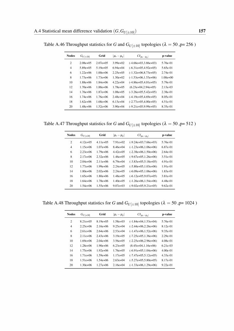
A.4 Statistical mean difference validation (G,GU [±10]) 157
Table A.46 Throughput statistics for G and GU [±10] topologies (λ = 50 ,p= 256 )
Nodes GU [±20] Grid |µr−µg| CI|µr−µg | p-value
2 2.08e+05 2.07e+05 3.99e+02 (-4.66e+03,3.86e+03) 5.76e-01
4 5.89e+05 5.19e+05 6.94e+04 (-6.31e+05,4.92e+05) 5.65e-01
6 1.22e+06 1.00e+06 2.25e+05 (-1.32e+06,8.73e+05) 2.74e-01
8 1.73e+06 1.73e+06 1.30e+02 (-1.53e+06,1.53e+06) 1.00e+00
10 1.88e+06 1.84e+06 4.22e+04 (-4.86e+05,4.01e+05) 5.79e-01
12 1.70e+06 1.88e+06 1.78e+05 (6.23e+04,2.94e+05) 2.13e-03
14 1.76e+06 1.87e+06 1.08e+05 (-3.26e+05,5.42e+05) 2.38e-01
16 1.74e+06 1.76e+06 2.48e+04 (-4.19e+05,4.69e+05) 8.05e-01
18 1.62e+06 1.68e+06 6.13e+04 (-2.77e+05,4.00e+05) 4.51e-01
20 1.48e+06 1.52e+06 3.90e+04 (-9.21e+05,9.99e+05) 8.35e-01
Table A.47 Throughput statistics for G and GU [±10] topologies (λ = 50 ,p= 512 )
Nodes GU [±20] Grid |µr−µg| CI|µr−µg | p-value
2 4.12e+05 4.11e+05 7.91e+02 (-9.24e+03,7.66e+03) 5.76e-01
4 1.15e+06 1.07e+06 8.46e+04 (-1.23e+06,1.06e+06) 6.87e-01
6 2.23e+06 1.79e+06 4.42e+05 (-2.38e+06,1.50e+06) 2.64e-01
8 2.17e+06 2.32e+06 1.46e+05 (-9.67e+05,1.26e+06) 3.51e-01
10 2.04e+06 2.11e+06 6.79e+04 (-3.83e+05,5.18e+05) 4.91e-01
12 1.77e+06 1.99e+06 2.24e+05 (-5.80e+05,1.03e+06) 1.91e-01
14 1.80e+06 2.02e+06 2.24e+05 (-6.09e+05,1.06e+06) 1.83e-01
16 1.65e+06 1.80e+06 1.48e+05 (-6.12e+05,9.07e+05) 3.81e-01
18 1.64e+06 1.78e+06 1.40e+05 (-1.26e+06,1.54e+06) 4.48e-01
20 1.54e+06 1.55e+06 9.07e+03 (-9.02e+05,9.21e+05) 9.62e-01
Table A.48 Throughput statistics for G and GU [±10] topologies (λ = 50 ,p= 1024 )
Nodes GU [±20] Grid |µr−µg| CI|µr−µg | p-value
2 8.21e+05 8.19e+05 1.58e+03 (-1.84e+04,1.53e+04) 5.76e-01
4 2.25e+06 2.16e+06 9.25e+04 (-2.44e+06,2.26e+06) 8.12e-01
6 2.61e+06 2.64e+06 2.53e+04 (-1.47e+06,1.52e+06) 9.35e-01
8 2.11e+06 2.43e+06 3.19e+05 (-7.25e+05,1.36e+06) 2.29e-01
10 1.69e+06 2.04e+06 3.56e+05 (-2.25e+06,2.96e+06) 4.08e-01
12 1.28e+06 1.90e+06 6.23e+05 (8.45e+04,1.16e+06) 6.21e-03
14 1.75e+06 1.92e+06 1.76e+05 (-6.91e+05,1.04e+06) 4.00e-01
16 1.71e+06 1.59e+06 1.17e+05 (-7.47e+05,5.12e+05) 4.33e-01
18 1.51e+06 1.54e+06 2.63e+04 (-5.27e+05,5.80e+05) 8.17e-01
20 1.30e+06 1.27e+06 2.16e+04 (-1.33e+06,1.29e+06) 9.22e-01

158 Statistical validation tables
Table A.49 Throughput statistics for G and GU [±10] topologies (λ = 100 ,p= 256 )
Nodes GU [±20] Grid |µr−µg| CI|µr−µg | p-value
2 4.16e+05 4.15e+05 1.12e+03 (-5.44e+03,3.20e+03) 2.88e-01
4 1.16e+06 1.04e+06 1.25e+05 (-1.18e+06,9.28e+05) 5.89e-01
6 2.20e+06 1.83e+06 3.69e+05 (-2.59e+06,1.85e+06) 3.64e-01
8 2.05e+06 2.13e+06 7.44e+04 (-6.53e+05,8.01e+05) 4.64e-01
10 1.87e+06 1.74e+06 1.24e+05 (-9.48e+05,7.00e+05) 5.22e-01
12 1.43e+06 1.75e+06 3.22e+05 (-5.62e+05,1.21e+06) 7.21e-02
14 1.44e+06 1.65e+06 2.13e+05 (-3.67e+05,7.94e+05) 1.66e-01
16 1.44e+06 1.46e+06 1.68e+04 (-4.54e+05,4.87e+05) 8.76e-01
18 1.42e+06 1.47e+06 5.10e+04 (-4.18e+05,5.20e+05) 6.42e-01
20 1.37e+06 1.27e+06 1.02e+05 (-1.66e+06,1.45e+06) 5.97e-01
Table A.50 Throughput statistics for G and GU [±10] topologies (λ = 100 ,p= 512 )
Nodes GU [±20] Grid |µr−µg| CI|µr−µg | p-value
2 8.26e+05 8.24e+05 2.22e+03 (-1.08e+04,6.34e+03) 2.88e-01
4 2.32e+06 2.05e+06 2.68e+05 (-1.79e+06,1.25e+06) 3.90e-01
6 2.69e+06 2.69e+06 2.30e+03 (-1.30e+06,1.30e+06) 9.93e-01
8 2.18e+06 2.38e+06 1.98e+05 (-1.09e+06,1.48e+06) 4.77e-01
10 1.97e+06 1.99e+06 1.33e+04 (-7.66e+05,7.93e+05) 9.32e-01
12 1.34e+06 1.82e+06 4.80e+05 (-1.28e+06,2.25e+06) 1.56e-01
14 1.62e+06 1.86e+06 2.42e+05 (-2.03e+05,6.86e+05) 5.67e-02
16 1.46e+06 1.61e+06 1.56e+05 (-9.55e+05,1.27e+06) 4.74e-01
18 1.45e+06 1.55e+06 9.57e+04 (-1.01e+06,1.20e+06) 6.79e-01
20 1.22e+06 1.32e+06 9.51e+04 (-1.03e+06,1.22e+06) 6.01e-01
Table A.51 Throughput statistics for G and GU [±10] topologies (λ = 100 ,p= 1024 )
Nodes GU [±20] Grid |µr−µg| CI|µr−µg | p-value
2 1.65e+06 1.64e+06 4.43e+03 (-2.15e+04,1.26e+04) 2.87e-01
4 3.09e+06 3.48e+06 3.91e+05 (-2.92e+06,3.70e+06) 4.40e-01
6 2.68e+06 2.39e+06 2.93e+05 (-2.81e+06,2.22e+06) 6.07e-01
8 2.28e+06 2.41e+06 1.32e+05 (-1.58e+06,1.85e+06) 7.37e-01
10 1.82e+06 1.90e+06 8.46e+04 (-2.05e+06,2.22e+06) 8.64e-01
12 1.47e+06 1.56e+06 8.55e+04 (-1.39e+06,1.56e+06) 8.03e-01
14 1.39e+06 1.63e+06 2.37e+05 (-2.93e+06,3.40e+06) 5.93e-01
16 1.09e+06 1.41e+06 3.20e+05 (-2.12e+06,2.75e+06) 5.10e-01
18 1.24e+06 1.36e+06 1.28e+05 (-4.63e+05,7.20e+05) 3.68e-01
20 1.28e+06 1.29e+06 8.94e+03 (-1.60e+06,1.62e+06) 9.74e-01
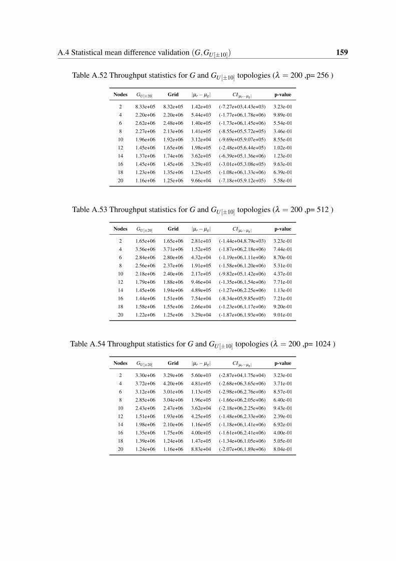
A.4 Statistical mean difference validation (G,GU [±10]) 159
Table A.52 Throughput statistics for G and GU [±10] topologies (λ = 200 ,p= 256 )
Nodes GU [±20] Grid |µr−µg| CI|µr−µg | p-value
2 8.33e+05 8.32e+05 1.42e+03 (-7.27e+03,4.43e+03) 3.23e-01
4 2.20e+06 2.20e+06 5.44e+03 (-1.77e+06,1.78e+06) 9.89e-01
6 2.62e+06 2.48e+06 1.40e+05 (-1.73e+06,1.45e+06) 5.54e-01
8 2.27e+06 2.13e+06 1.41e+05 (-8.55e+05,5.72e+05) 3.46e-01
10 1.96e+06 1.92e+06 3.12e+04 (-9.69e+05,9.07e+05) 8.55e-01
12 1.45e+06 1.65e+06 1.98e+05 (-2.48e+05,6.44e+05) 1.02e-01
14 1.37e+06 1.74e+06 3.62e+05 (-6.39e+05,1.36e+06) 1.23e-01
16 1.45e+06 1.45e+06 3.29e+03 (-3.01e+05,3.08e+05) 9.63e-01
18 1.23e+06 1.35e+06 1.23e+05 (-1.08e+06,1.33e+06) 6.39e-01
20 1.16e+06 1.25e+06 9.66e+04 (-7.18e+05,9.12e+05) 5.58e-01
Table A.53 Throughput statistics for G and GU [±10] topologies (λ = 200 ,p= 512 )
Nodes GU [±20] Grid |µr−µg| CI|µr−µg | p-value
2 1.65e+06 1.65e+06 2.81e+03 (-1.44e+04,8.79e+03) 3.23e-01
4 3.56e+06 3.71e+06 1.52e+05 (-1.87e+06,2.18e+06) 7.44e-01
6 2.84e+06 2.80e+06 4.32e+04 (-1.19e+06,1.11e+06) 8.70e-01
8 2.56e+06 2.37e+06 1.91e+05 (-1.58e+06,1.20e+06) 5.31e-01
10 2.18e+06 2.40e+06 2.17e+05 (-9.82e+05,1.42e+06) 4.37e-01
12 1.79e+06 1.88e+06 9.46e+04 (-1.35e+06,1.54e+06) 7.71e-01
14 1.45e+06 1.94e+06 4.89e+05 (-1.27e+06,2.25e+06) 1.13e-01
16 1.44e+06 1.51e+06 7.54e+04 (-8.34e+05,9.85e+05) 7.21e-01
18 1.58e+06 1.55e+06 2.66e+04 (-1.23e+06,1.17e+06) 9.20e-01
20 1.22e+06 1.25e+06 3.29e+04 (-1.87e+06,1.93e+06) 9.01e-01
Table A.54 Throughput statistics for G and GU [±10] topologies (λ = 200 ,p= 1024 )
Nodes GU [±20] Grid |µr−µg| CI|µr−µg | p-value
2 3.30e+06 3.29e+06 5.60e+03 (-2.87e+04,1.75e+04) 3.23e-01
4 3.72e+06 4.20e+06 4.81e+05 (-2.68e+06,3.65e+06) 3.71e-01
6 3.12e+06 3.01e+06 1.13e+05 (-2.98e+06,2.76e+06) 8.57e-01
8 2.85e+06 3.04e+06 1.96e+05 (-1.66e+06,2.05e+06) 6.40e-01
10 2.43e+06 2.47e+06 3.62e+04 (-2.18e+06,2.25e+06) 9.43e-01
12 1.51e+06 1.93e+06 4.25e+05 (-1.48e+06,2.33e+06) 2.39e-01
14 1.98e+06 2.10e+06 1.16e+05 (-1.18e+06,1.41e+06) 6.92e-01
16 1.35e+06 1.75e+06 4.00e+05 (-1.61e+06,2.41e+06) 4.00e-01
18 1.39e+06 1.24e+06 1.47e+05 (-1.34e+06,1.05e+06) 5.05e-01
20 1.24e+06 1.16e+06 8.83e+04 (-2.07e+06,1.89e+06) 8.04e-01

160 Statistical validation tables
Table A.55 Delay statistics for G and GU [±10] topologies (λ = 10 ,p= 256 )
Nodes GU [±20] Grid |µr−µg| CI|µr−µg | p-value
2 3.19e-04 3.11e-04 8.53e-06 (-8.21e-05,6.51e-05) 3.70e-01
4 4.86e-04 4.49e-04 3.70e-05 (-6.81e-04,6.07e-04) 7.21e-01
6 8.47e-04 5.61e-04 2.86e-04 (-9.89e-04,4.17e-04) 1.09e-01
8 1.17e-03 9.17e-04 2.49e-04 (-1.70e-03,1.20e-03) 4.36e-01
10 1.30e-03 1.29e-03 8.49e-06 (-1.01e-03,9.90e-04) 9.71e-01
12 1.74e-03 1.67e-03 7.30e-05 (-7.46e-04,6.00e-04) 5.87e-01
14 2.08e-03 2.52e-03 4.39e-04 (-3.32e-03,4.19e-03) 3.76e-01
16 2.60e-03 2.18e-03 4.14e-04 (-3.12e-03,2.29e-03) 2.96e-01
18 2.99e-03 2.56e-03 4.25e-04 (-1.62e-03,7.67e-04) 1.76e-01
20 3.55e-03 3.48e-03 7.36e-05 (-6.66e-03,6.52e-03) 9.45e-01
Table A.56 Delay statistics for G and GU [±10] topologies (λ = 10 ,p= 512 )
Nodes GU [±20] Grid |µr−µg| CI|µr−µg | p-value
2 5.11e-04 4.90e-04 2.04e-05 (-1.97e-04,1.56e-04) 3.70e-01
4 8.19e-04 7.44e-04 7.51e-05 (-1.43e-03,1.28e-03) 7.01e-01
6 1.59e-03 1.03e-03 5.54e-04 (-2.10e-03,9.95e-04) 1.15e-01
8 2.55e-03 1.68e-03 8.65e-04 (-3.74e-03,2.01e-03) 1.85e-01
10 2.75e-03 3.35e-03 5.99e-04 (-5.76e-03,6.96e-03) 5.20e-01
12 3.42e-03 3.94e-03 5.21e-04 (-3.94e-03,4.98e-03) 5.28e-01
14 4.66e-03 5.61e-03 9.50e-04 (-4.87e-03,6.77e-03) 3.18e-01
16 5.87e-03 6.24e-03 3.66e-04 (-3.08e-03,3.81e-03) 6.50e-01
18 7.35e-03 6.08e-03 1.27e-03 (-6.38e-03,3.84e-03) 3.16e-01
20 7.64e-03 1.07e-02 3.03e-03 (-3.65e-02,4.26e-02) 5.52e-01
Table A.57 Delay statistics for G and GU [±10] topologies (λ = 10 ,p= 1024 )
Nodes GU [±20] Grid |µr−µg| CI|µr−µg | p-value
2 9.15e-04 8.55e-04 6.06e-05 (-5.82e-04,4.61e-04) 3.68e-01
4 1.67e-03 1.38e-03 2.89e-04 (-2.52e-03,1.94e-03) 5.25e-01
6 3.45e-03 2.53e-03 9.17e-04 (-5.01e-03,3.18e-03) 3.43e-01
8 5.43e-03 3.61e-03 1.82e-03 (-7.86e-03,4.21e-03) 1.84e-01
10 6.54e-03 5.59e-03 9.54e-04 (-5.80e-03,3.89e-03) 4.16e-01
12 7.81e-03 8.38e-03 5.73e-04 (-5.61e-03,6.76e-03) 4.62e-01
14 1.86e-02 2.13e-02 2.75e-03 (-2.95e-02,3.50e-02) 5.79e-01
16 3.18e-02 2.20e-02 9.87e-03 (-5.26e-02,3.29e-02) 3.05e-01
18 3.54e-02 2.85e-02 6.95e-03 (-6.27e-02,4.88e-02) 3.93e-01
20 4.17e-02 3.71e-02 4.61e-03 (-5.66e-02,4.74e-02) 6.60e-01
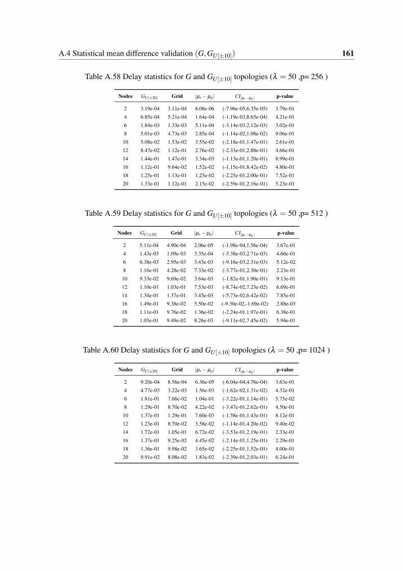
A.4 Statistical mean difference validation (G,GU [±10]) 161
Table A.58 Delay statistics for G and GU [±10] topologies (λ = 50 ,p= 256 )
Nodes GU [±20] Grid |µr−µg| CI|µr−µg | p-value
2 3.19e-04 3.11e-04 8.08e-06 (-7.96e-05,6.35e-05) 3.79e-01
4 6.85e-04 5.21e-04 1.64e-04 (-1.19e-03,8.65e-04) 4.21e-01
6 1.84e-03 1.33e-03 5.11e-04 (-3.14e-03,2.12e-03) 3.02e-01
8 5.01e-03 4.73e-03 2.85e-04 (-1.14e-02,1.08e-02) 9.06e-01
10 5.08e-02 1.53e-02 3.55e-02 (-2.18e-01,1.47e-01) 2.61e-01
12 8.47e-02 1.12e-01 2.76e-02 (-2.33e-01,2.88e-01) 4.66e-01
14 1.44e-01 1.47e-01 3.34e-03 (-1.13e-01,1.20e-01) 8.99e-01
16 1.12e-01 9.64e-02 1.52e-02 (-1.15e-01,8.42e-02) 4.80e-01
18 1.25e-01 1.13e-01 1.25e-02 (-2.25e-01,2.00e-01) 7.52e-01
20 1.33e-01 1.12e-01 2.15e-02 (-2.59e-01,2.16e-01) 5.23e-01
Table A.59 Delay statistics for G and GU [±10] topologies (λ = 50 ,p= 512 )
Nodes GU [±20] Grid |µr−µg| CI|µr−µg | p-value
2 5.11e-04 4.90e-04 2.06e-05 (-1.98e-04,1.56e-04) 3.67e-01
4 1.43e-03 1.09e-03 3.35e-04 (-3.38e-03,2.71e-03) 4.66e-01
6 6.38e-03 2.95e-03 3.43e-03 (-9.16e-03,2.31e-03) 5.12e-02
8 1.16e-01 4.28e-02 7.33e-02 (-3.77e-01,2.30e-01) 2.23e-01
10 9.33e-02 9.69e-02 3.64e-03 (-1.82e-01,1.90e-01) 9.13e-01
12 1.10e-01 1.03e-01 7.53e-03 (-8.74e-02,7.23e-02) 6.69e-01
14 1.34e-01 1.37e-01 3.45e-03 (-5.73e-02,6.42e-02) 7.85e-01
16 1.49e-01 9.38e-02 5.50e-02 (-9.30e-02,-1.69e-02) 2.88e-03
18 1.11e-01 9.76e-02 1.36e-02 (-2.24e-01,1.97e-01) 6.38e-01
20 1.03e-01 9.49e-02 8.26e-03 (-9.11e-02,7.45e-02) 5.94e-01
Table A.60 Delay statistics for G and GU [±10] topologies (λ = 50 ,p= 1024 )
Nodes GU [±20] Grid |µr−µg| CI|µr−µg | p-value
2 9.20e-04 8.56e-04 6.36e-05 (-6.04e-04,4.76e-04) 3.63e-01
4 4.77e-03 3.22e-03 1.56e-03 (-1.62e-02,1.31e-02) 4.32e-01
6 1.81e-01 7.66e-02 1.04e-01 (-3.22e-01,1.14e-01) 5.75e-02
8 1.29e-01 8.70e-02 4.22e-02 (-3.47e-01,2.62e-01) 4.50e-01
10 1.37e-01 1.29e-01 7.60e-03 (-1.58e-01,1.43e-01) 8.12e-01
12 1.23e-01 8.70e-02 3.58e-02 (-1.14e-01,4.20e-02) 9.40e-02
14 1.72e-01 1.05e-01 6.72e-02 (-3.53e-01,2.19e-01) 2.33e-01
16 1.37e-01 9.25e-02 4.45e-02 (-2.14e-01,1.25e-01) 2.29e-01
18 1.36e-01 9.98e-02 3.65e-02 (-2.25e-01,1.52e-01) 4.00e-01
20 9.91e-02 8.08e-02 1.83e-02 (-2.39e-01,2.03e-01) 6.24e-01

162 Statistical validation tables
Table A.61 Delay statistics for G and GU [±10] topologies (λ = 100 ,p= 256 )
Nodes GU [±20] Grid |µr−µg| CI|µr−µg | p-value
2 3.19e-04 3.11e-04 8.56e-06 (-8.25e-05,6.54e-05) 3.70e-01
4 1.09e-03 7.22e-04 3.72e-04 (-3.60e-03,2.86e-03) 4.77e-01
6 1.20e-02 4.89e-03 7.09e-03 (-3.31e-02,1.89e-02) 2.13e-01
8 3.35e-01 1.70e-01 1.64e-01 (-8.94e-01,5.66e-01) 3.34e-01
10 2.22e-01 2.08e-01 1.47e-02 (-3.26e-01,2.97e-01) 8.13e-01
12 2.26e-01 2.06e-01 1.93e-02 (-2.17e-01,1.79e-01) 6.76e-01
14 2.68e-01 2.52e-01 1.54e-02 (-8.92e-02,5.85e-02) 3.91e-01
16 2.22e-01 1.57e-01 6.57e-02 (-1.99e-01,6.76e-02) 7.08e-02
18 1.48e-01 1.19e-01 2.86e-02 (-1.39e-01,8.16e-02) 2.86e-01
20 1.47e-01 1.65e-01 1.83e-02 (-8.87e-02,1.25e-01) 4.74e-01
Table A.62 Delay statistics for G and GU [±10] topologies (λ = 100 ,p= 512 )
Nodes GU [±20] Grid |µr−µg| CI|µr−µg | p-value
2 5.12e-04 4.92e-04 2.07e-05 (-2.04e-04,1.62e-04) 3.78e-01
4 3.84e-03 1.90e-03 1.94e-03 (-7.17e-03,3.30e-03) 1.31e-01
6 3.50e-01 2.39e-01 1.11e-01 (-9.09e-01,6.87e-01) 4.08e-01
8 2.12e-01 1.78e-01 3.34e-02 (-3.93e-01,3.26e-01) 6.69e-01
10 2.00e-01 1.53e-01 4.74e-02 (-2.36e-01,1.42e-01) 2.53e-01
12 1.99e-01 1.21e-01 7.77e-02 (-3.90e-01,2.34e-01) 1.74e-01
14 1.96e-01 1.86e-01 1.01e-02 (-4.83e-01,4.63e-01) 8.57e-01
16 1.78e-01 1.28e-01 5.01e-02 (-2.66e-01,1.66e-01) 2.67e-01
18 1.38e-01 1.27e-01 1.12e-02 (-1.62e-01,1.40e-01) 7.34e-01
20 1.12e-01 1.17e-01 4.77e-03 (-1.18e-01,1.27e-01) 8.40e-01
Table A.63 Delay statistics for G and GU [±10] topologies (λ = 100 ,p= 1024 )
Nodes GU [±20] Grid |µr−µg| CI|µr−µg | p-value
2 9.26e-04 8.60e-04 6.56e-05 (-6.33e-04,5.02e-04) 3.70e-01
4 3.24e-01 2.17e-01 1.07e-01 (-1.06e+00,8.50e-01) 5.82e-01
6 2.89e-01 1.59e-01 1.30e-01 (-4.76e-01,2.15e-01) 1.39e-01
8 2.31e-01 1.19e-01 1.12e-01 (-6.76e-01,4.52e-01) 2.96e-01
10 1.92e-01 1.22e-01 7.03e-02 (-2.25e-01,8.48e-02) 9.57e-02
12 1.91e-01 1.01e-01 9.02e-02 (-2.97e-01,1.17e-01) 8.14e-02
14 1.88e-01 1.83e-01 4.99e-03 (-1.66e-01,1.56e-01) 8.92e-01
16 1.88e-01 1.25e-01 6.31e-02 (-3.99e-01,2.73e-01) 3.70e-01
18 1.43e-01 8.53e-02 5.75e-02 (-2.61e-01,1.46e-01) 2.27e-01
20 7.55e-02 9.83e-02 2.28e-02 (-1.53e-01,1.98e-01) 5.82e-01

A.4 Statistical mean difference validation (G,GU [±10]) 163
Table A.64 Delay statistics for G and GU [±10] topologies (λ = 200 ,p= 256 )
Nodes GU [±20] Grid |µr−µg| CI|µr−µg | p-value
2 3.21e-04 3.12e-04 9.08e-06 (-8.80e-05,6.98e-05) 3.72e-01
4 3.37e-03 2.27e-03 1.10e-03 (-1.31e-02,1.09e-02) 6.08e-01
6 3.37e-01 3.07e-01 2.92e-02 (-6.22e-01,5.64e-01) 7.14e-01
8 2.62e-01 2.15e-01 4.72e-02 (-3.74e-01,2.79e-01) 4.94e-01
10 2.61e-01 1.95e-01 6.56e-02 (-1.30e-01,-6.98e-04) 9.70e-03
12 1.99e-01 2.17e-01 1.80e-02 (-4.88e-01,5.24e-01) 7.71e-01
14 2.95e-01 2.45e-01 5.00e-02 (-3.36e-01,2.35e-01) 3.30e-01
16 2.01e-01 1.63e-01 3.82e-02 (-2.35e-01,1.59e-01) 2.74e-01
18 1.91e-01 1.42e-01 4.93e-02 (-3.70e-01,2.71e-01) 4.13e-01
20 1.70e-01 1.64e-01 6.00e-03 (-2.99e-01,2.87e-01) 9.03e-01
Table A.65 Delay statistics for G and GU [±10] topologies (λ = 200 ,p= 512 )
Nodes GU [±20] Grid |µr−µg| CI|µr−µg | p-value
2 5.17e-04 4.94e-04 2.29e-05 (-2.24e-04,1.78e-04) 3.75e-01
4 2.39e-01 2.24e-01 1.44e-02 (-9.15e-01,8.86e-01) 9.44e-01
6 2.95e-01 1.47e-01 1.48e-01 (-4.59e-01,1.63e-01) 8.23e-02
8 2.06e-01 1.39e-01 6.68e-02 (-5.29e-01,3.95e-01) 4.62e-01
10 1.79e-01 1.80e-01 1.62e-03 (-1.30e-01,1.33e-01) 9.42e-01
12 1.92e-01 1.60e-01 3.14e-02 (-4.36e-01,3.73e-01) 6.53e-01
14 2.06e-01 1.68e-01 3.80e-02 (-1.98e-01,1.22e-01) 3.22e-01
16 2.28e-01 1.24e-01 1.04e-01 (-3.08e-01,9.93e-02) 7.55e-02
18 1.87e-01 1.07e-01 7.93e-02 (-6.70e-01,5.11e-01) 3.37e-01
20 1.23e-01 1.25e-01 2.35e-03 (-2.89e-01,2.94e-01) 9.59e-01
Table A.66 Delay statistics for G and GU [±10] topologies (λ = 200 ,p= 1024 )
Nodes GU [±20] Grid |µr−µg| CI|µr−µg | p-value
2 9.49e-04 8.73e-04 7.61e-05 (-7.26e-04,5.74e-04) 3.66e-01
4 1.34e-01 1.65e-01 3.07e-02 (-1.50e-01,2.11e-01) 4.71e-01
6 2.43e-01 1.55e-01 8.76e-02 (-4.45e-01,2.70e-01) 1.73e-01
8 3.22e-01 1.18e-01 2.04e-01 (-1.50e+00,1.10e+00) 3.14e-01
10 3.03e-01 1.37e-01 1.66e-01 (-1.34e+00,1.00e+00) 3.78e-01
12 1.91e-01 1.10e-01 8.10e-02 (-2.76e-01,1.15e-01) 1.27e-01
14 2.65e-01 1.68e-01 9.69e-02 (-8.19e-01,6.25e-01) 4.32e-01
16 1.81e-01 2.02e-01 2.08e-02 (-4.32e-01,4.73e-01) 8.39e-01
18 2.36e-01 1.39e-01 9.66e-02 (-4.69e-01,2.76e-01) 2.36e-01
20 1.58e-01 8.69e-02 7.08e-02 (-6.45e-01,5.03e-01) 4.56e-01
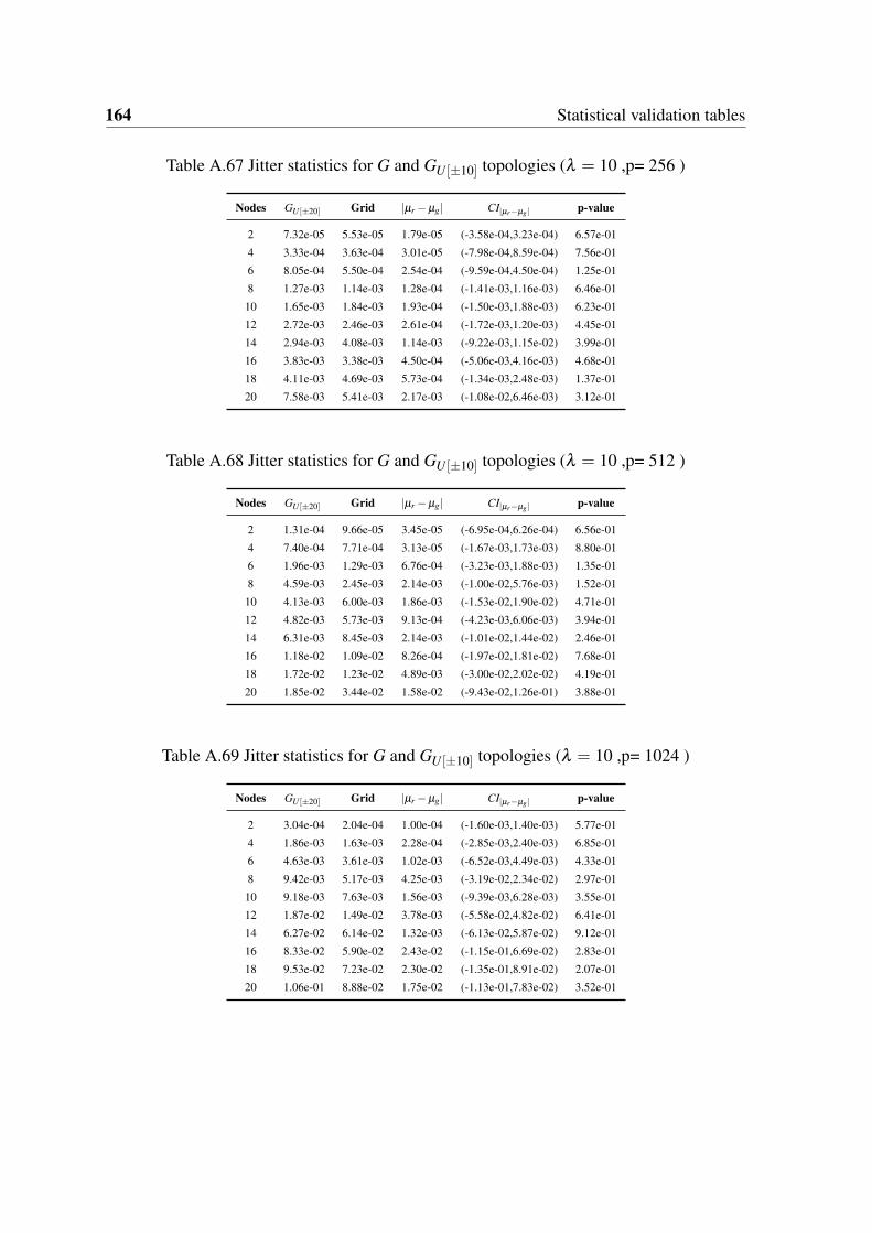
164 Statistical validation tables
Table A.67 Jitter statistics for G and GU [±10] topologies (λ = 10 ,p= 256 )
Nodes GU [±20] Grid |µr−µg| CI|µr−µg | p-value
2 7.32e-05 5.53e-05 1.79e-05 (-3.58e-04,3.23e-04) 6.57e-01
4 3.33e-04 3.63e-04 3.01e-05 (-7.98e-04,8.59e-04) 7.56e-01
6 8.05e-04 5.50e-04 2.54e-04 (-9.59e-04,4.50e-04) 1.25e-01
8 1.27e-03 1.14e-03 1.28e-04 (-1.41e-03,1.16e-03) 6.46e-01
10 1.65e-03 1.84e-03 1.93e-04 (-1.50e-03,1.88e-03) 6.23e-01
12 2.72e-03 2.46e-03 2.61e-04 (-1.72e-03,1.20e-03) 4.45e-01
14 2.94e-03 4.08e-03 1.14e-03 (-9.22e-03,1.15e-02) 3.99e-01
16 3.83e-03 3.38e-03 4.50e-04 (-5.06e-03,4.16e-03) 4.68e-01
18 4.11e-03 4.69e-03 5.73e-04 (-1.34e-03,2.48e-03) 1.37e-01
20 7.58e-03 5.41e-03 2.17e-03 (-1.08e-02,6.46e-03) 3.12e-01
Table A.68 Jitter statistics for G and GU [±10] topologies (λ = 10 ,p= 512 )
Nodes GU [±20] Grid |µr−µg| CI|µr−µg | p-value
2 1.31e-04 9.66e-05 3.45e-05 (-6.95e-04,6.26e-04) 6.56e-01
4 7.40e-04 7.71e-04 3.13e-05 (-1.67e-03,1.73e-03) 8.80e-01
6 1.96e-03 1.29e-03 6.76e-04 (-3.23e-03,1.88e-03) 1.35e-01
8 4.59e-03 2.45e-03 2.14e-03 (-1.00e-02,5.76e-03) 1.52e-01
10 4.13e-03 6.00e-03 1.86e-03 (-1.53e-02,1.90e-02) 4.71e-01
12 4.82e-03 5.73e-03 9.13e-04 (-4.23e-03,6.06e-03) 3.94e-01
14 6.31e-03 8.45e-03 2.14e-03 (-1.01e-02,1.44e-02) 2.46e-01
16 1.18e-02 1.09e-02 8.26e-04 (-1.97e-02,1.81e-02) 7.68e-01
18 1.72e-02 1.23e-02 4.89e-03 (-3.00e-02,2.02e-02) 4.19e-01
20 1.85e-02 3.44e-02 1.58e-02 (-9.43e-02,1.26e-01) 3.88e-01
Table A.69 Jitter statistics for G and GU [±10] topologies (λ = 10 ,p= 1024 )
Nodes GU [±20] Grid |µr−µg| CI|µr−µg | p-value
2 3.04e-04 2.04e-04 1.00e-04 (-1.60e-03,1.40e-03) 5.77e-01
4 1.86e-03 1.63e-03 2.28e-04 (-2.85e-03,2.40e-03) 6.85e-01
6 4.63e-03 3.61e-03 1.02e-03 (-6.52e-03,4.49e-03) 4.33e-01
8 9.42e-03 5.17e-03 4.25e-03 (-3.19e-02,2.34e-02) 2.97e-01
10 9.18e-03 7.63e-03 1.56e-03 (-9.39e-03,6.28e-03) 3.55e-01
12 1.87e-02 1.49e-02 3.78e-03 (-5.58e-02,4.82e-02) 6.41e-01
14 6.27e-02 6.14e-02 1.32e-03 (-6.13e-02,5.87e-02) 9.12e-01
16 8.33e-02 5.90e-02 2.43e-02 (-1.15e-01,6.69e-02) 2.83e-01
18 9.53e-02 7.23e-02 2.30e-02 (-1.35e-01,8.91e-02) 2.07e-01
20 1.06e-01 8.88e-02 1.75e-02 (-1.13e-01,7.83e-02) 3.52e-01

A.4 Statistical mean difference validation (G,GU [±10]) 165
Table A.70 Jitter statistics for G and GU [±10] topologies (λ = 50 ,p= 256 )
Nodes GU [±20] Grid |µr−µg| CI|µr−µg | p-value
2 7.45e-05 5.48e-05 1.96e-05 (-3.53e-04,3.14e-04) 6.18e-01
4 9.31e-04 6.99e-04 2.32e-04 (-1.80e-03,1.34e-03) 4.33e-01
6 3.01e-03 3.16e-03 1.51e-04 (-7.78e-03,8.08e-03) 8.96e-01
8 1.00e-02 7.95e-03 2.06e-03 (-2.00e-02,1.59e-02) 6.25e-01
10 1.28e-01 5.60e-02 7.24e-02 (-4.45e-01,3.01e-01) 3.17e-01
12 2.42e-01 2.62e-01 2.05e-02 (-3.62e-01,4.04e-01) 7.09e-01
14 3.58e-01 3.28e-01 2.98e-02 (-2.35e-01,1.76e-01) 4.83e-01
16 2.88e-01 2.44e-01 4.46e-02 (-3.09e-01,2.19e-01) 3.58e-01
18 3.18e-01 2.82e-01 3.59e-02 (-3.40e-01,2.68e-01) 5.69e-01
20 3.28e-01 2.84e-01 4.38e-02 (-4.84e-01,3.96e-01) 4.48e-01
Table A.71 Jitter statistics for G and GU [±10] topologies (λ = 50 ,p= 512 )
Nodes GU [±20] Grid |µr−µg| CI|µr−µg | p-value
2 1.39e-04 9.98e-05 3.93e-05 (-6.83e-04,6.05e-04) 6.07e-01
4 2.24e-03 1.85e-03 3.83e-04 (-6.08e-03,5.31e-03) 5.78e-01
6 1.43e-02 4.84e-03 9.45e-03 (-4.96e-02,3.07e-02) 1.82e-01
8 2.77e-01 1.23e-01 1.54e-01 (-6.43e-01,3.35e-01) 1.51e-01
10 2.53e-01 2.59e-01 6.19e-03 (-3.69e-01,3.82e-01) 9.28e-01
12 3.68e-01 3.06e-01 6.28e-02 (-2.90e-01,1.65e-01) 2.05e-01
14 4.22e-01 3.90e-01 3.20e-02 (-2.13e-01,1.49e-01) 4.42e-01
16 4.33e-01 3.06e-01 1.27e-01 (-2.46e-01,-7.98e-03) 7.97e-03
18 3.60e-01 2.89e-01 7.06e-02 (-3.69e-01,2.28e-01) 1.77e-01
20 3.29e-01 3.10e-01 1.93e-02 (-5.12e-02,1.26e-02) 4.31e-02
Table A.72 Jitter statistics for G and GU [±10] topologies (λ = 50 ,p= 1024 )
Nodes GU [±20] Grid |µr−µg| CI|µr−µg | p-value
2 3.17e-04 2.12e-04 1.05e-04 (-1.55e-03,1.34e-03) 5.45e-01
4 8.75e-03 5.77e-03 2.99e-03 (-3.51e-02,2.91e-02) 4.54e-01
6 4.85e-01 2.23e-01 2.61e-01 (-7.16e-01,1.94e-01) 5.71e-02
8 4.92e-01 3.28e-01 1.64e-01 (-9.48e-01,6.20e-01) 2.80e-01
10 6.58e-01 5.08e-01 1.50e-01 (-8.77e-01,5.77e-01) 3.21e-01
12 6.35e-01 3.94e-01 2.41e-01 (-4.86e-01,4.28e-03) 1.04e-02
14 6.36e-01 4.08e-01 2.28e-01 (-1.32e+00,8.64e-01) 2.05e-01
16 4.97e-01 4.09e-01 8.79e-02 (-3.66e-01,1.90e-01) 2.08e-01
18 5.57e-01 3.80e-01 1.77e-01 (-5.07e-01,1.52e-01) 5.85e-02
20 4.18e-01 3.87e-01 3.08e-02 (-1.12e+00,1.06e+00) 8.12e-01

166 Statistical validation tables
Table A.73 Jitter statistics for G and GU [±10] topologies (λ = 100 ,p= 256 )
Nodes GU [±20] Grid |µr−µg| CI|µr−µg | p-value
2 7.99e-05 5.81e-05 2.18e-05 (-3.64e-04,3.20e-04) 5.93e-01
4 1.79e-03 1.25e-03 5.40e-04 (-5.90e-03,4.82e-03) 5.31e-01
6 3.83e-02 1.12e-02 2.71e-02 (-1.42e-01,8.81e-02) 2.04e-01
8 6.62e-01 3.70e-01 2.92e-01 (-1.27e+00,6.87e-01) 2.40e-01
10 5.68e-01 6.30e-01 6.20e-02 (-7.98e-01,9.22e-01) 6.38e-01
12 6.79e-01 5.51e-01 1.28e-01 (-6.95e-01,4.39e-01) 2.49e-01
14 7.69e-01 6.48e-01 1.21e-01 (-3.92e-01,1.50e-01) 1.04e-01
16 5.76e-01 4.80e-01 9.63e-02 (-2.76e-01,8.39e-02) 6.66e-02
18 4.76e-01 3.82e-01 9.38e-02 (-4.91e-01,3.04e-01) 1.89e-01
20 4.47e-01 5.00e-01 5.23e-02 (-2.88e-01,3.93e-01) 4.98e-01
Table A.74 Jitter statistics for G and GU [±10] topologies (λ = 100 ,p= 512 )
Nodes GU [±20] Grid |µr−µg| CI|µr−µg | p-value
2 1.49e-04 1.08e-04 4.13e-05 (-6.75e-04,5.93e-04) 5.85e-01
4 7.90e-03 3.51e-03 4.39e-03 (-1.76e-02,8.77e-03) 1.28e-01
6 7.72e-01 5.46e-01 2.26e-01 (-1.97e+00,1.52e+00) 3.59e-01
8 6.77e-01 5.43e-01 1.34e-01 (-5.16e-01,2.49e-01) 1.80e-01
10 6.92e-01 6.31e-01 6.08e-02 (-5.09e-01,3.87e-01) 4.06e-01
12 7.90e-01 5.36e-01 2.54e-01 (-6.82e-01,1.74e-01) 3.56e-02
14 7.09e-01 6.34e-01 7.48e-02 (-8.97e-01,7.48e-01) 5.54e-01
16 6.11e-01 4.87e-01 1.24e-01 (-9.87e-01,7.39e-01) 3.73e-01
18 5.35e-01 4.78e-01 5.75e-02 (-2.93e-01,1.78e-01) 2.72e-01
20 4.98e-01 4.41e-01 5.74e-02 (-4.89e-01,3.74e-01) 4.05e-01
Table A.75 Jitter statistics for G and GU [±10] topologies (λ = 100 ,p= 1024 )
Nodes GU [±20] Grid |µr−µg| CI|µr−µg | p-value
2 3.49e-04 2.36e-04 1.13e-04 (-1.60e-03,1.38e-03) 5.31e-01
4 9.98e-01 6.14e-01 3.84e-01 (-2.06e+00,1.29e+00) 2.66e-01
6 9.49e-01 7.43e-01 2.06e-01 (-4.74e-01,6.12e-02) 1.81e-02
8 7.79e-01 5.65e-01 2.14e-01 (-1.08e+00,6.48e-01) 2.79e-01
10 8.57e-01 6.81e-01 1.76e-01 (-4.40e-01,8.75e-02) 3.70e-02
12 8.28e-01 5.95e-01 2.32e-01 (-5.24e-01,5.96e-02) 2.14e-02
14 8.44e-01 7.23e-01 1.21e-01 (-8.51e-01,6.09e-01) 4.58e-01
16 7.83e-01 6.17e-01 1.66e-01 (-1.39e+00,1.06e+00) 4.51e-01
18 5.77e-01 4.41e-01 1.36e-01 (-6.08e-01,3.37e-01) 2.07e-01
20 4.25e-01 4.83e-01 5.74e-02 (-3.25e-01,4.40e-01) 4.64e-01
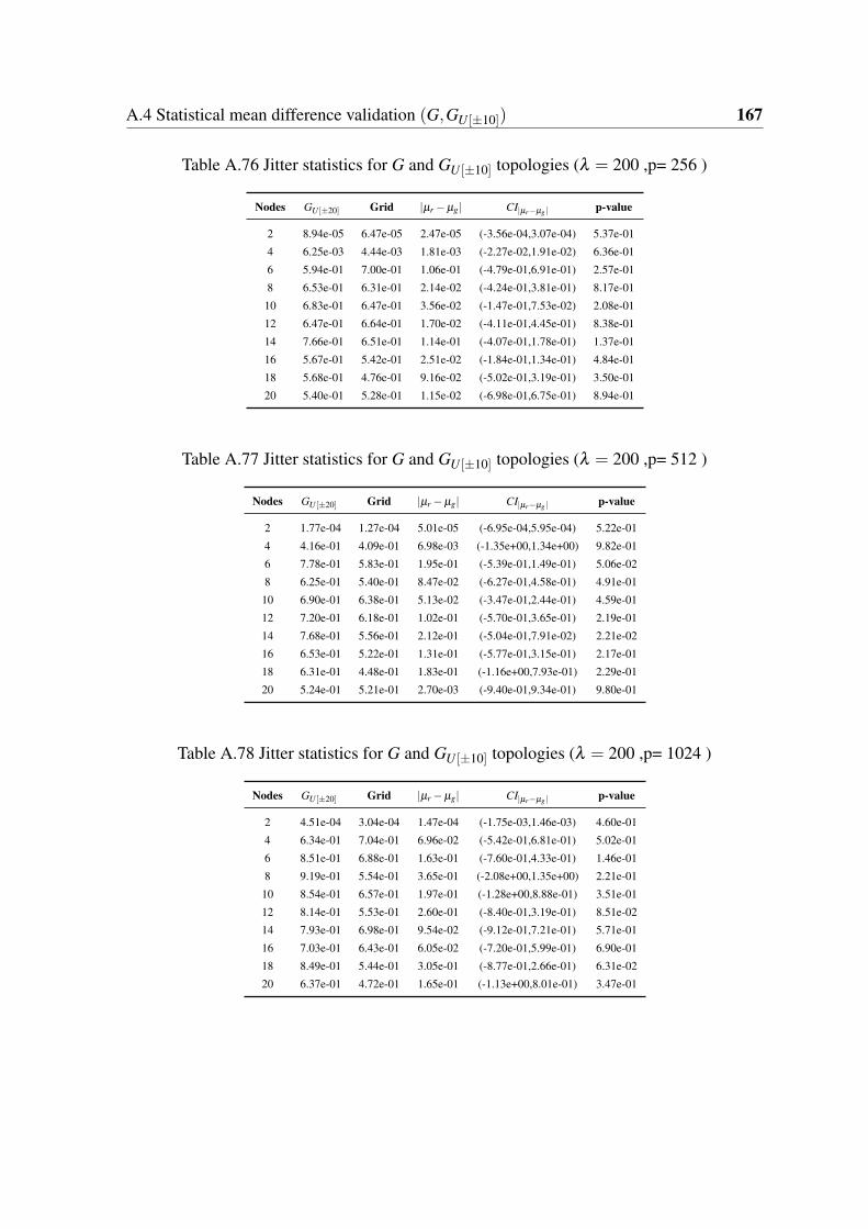
A.4 Statistical mean difference validation (G,GU [±10]) 167
Table A.76 Jitter statistics for G and GU [±10] topologies (λ = 200 ,p= 256 )
Nodes GU [±20] Grid |µr−µg| CI|µr−µg | p-value
2 8.94e-05 6.47e-05 2.47e-05 (-3.56e-04,3.07e-04) 5.37e-01
4 6.25e-03 4.44e-03 1.81e-03 (-2.27e-02,1.91e-02) 6.36e-01
6 5.94e-01 7.00e-01 1.06e-01 (-4.79e-01,6.91e-01) 2.57e-01
8 6.53e-01 6.31e-01 2.14e-02 (-4.24e-01,3.81e-01) 8.17e-01
10 6.83e-01 6.47e-01 3.56e-02 (-1.47e-01,7.53e-02) 2.08e-01
12 6.47e-01 6.64e-01 1.70e-02 (-4.11e-01,4.45e-01) 8.38e-01
14 7.66e-01 6.51e-01 1.14e-01 (-4.07e-01,1.78e-01) 1.37e-01
16 5.67e-01 5.42e-01 2.51e-02 (-1.84e-01,1.34e-01) 4.84e-01
18 5.68e-01 4.76e-01 9.16e-02 (-5.02e-01,3.19e-01) 3.50e-01
20 5.40e-01 5.28e-01 1.15e-02 (-6.98e-01,6.75e-01) 8.94e-01
Table A.77 Jitter statistics for G and GU [±10] topologies (λ = 200 ,p= 512 )
Nodes GU [±20] Grid |µr−µg| CI|µr−µg | p-value
2 1.77e-04 1.27e-04 5.01e-05 (-6.95e-04,5.95e-04) 5.22e-01
4 4.16e-01 4.09e-01 6.98e-03 (-1.35e+00,1.34e+00) 9.82e-01
6 7.78e-01 5.83e-01 1.95e-01 (-5.39e-01,1.49e-01) 5.06e-02
8 6.25e-01 5.40e-01 8.47e-02 (-6.27e-01,4.58e-01) 4.91e-01
10 6.90e-01 6.38e-01 5.13e-02 (-3.47e-01,2.44e-01) 4.59e-01
12 7.20e-01 6.18e-01 1.02e-01 (-5.70e-01,3.65e-01) 2.19e-01
14 7.68e-01 5.56e-01 2.12e-01 (-5.04e-01,7.91e-02) 2.21e-02
16 6.53e-01 5.22e-01 1.31e-01 (-5.77e-01,3.15e-01) 2.17e-01
18 6.31e-01 4.48e-01 1.83e-01 (-1.16e+00,7.93e-01) 2.29e-01
20 5.24e-01 5.21e-01 2.70e-03 (-9.40e-01,9.34e-01) 9.80e-01
Table A.78 Jitter statistics for G and GU [±10] topologies (λ = 200 ,p= 1024 )
Nodes GU [±20] Grid |µr−µg| CI|µr−µg | p-value
2 4.51e-04 3.04e-04 1.47e-04 (-1.75e-03,1.46e-03) 4.60e-01
4 6.34e-01 7.04e-01 6.96e-02 (-5.42e-01,6.81e-01) 5.02e-01
6 8.51e-01 6.88e-01 1.63e-01 (-7.60e-01,4.33e-01) 1.46e-01
8 9.19e-01 5.54e-01 3.65e-01 (-2.08e+00,1.35e+00) 2.21e-01
10 8.54e-01 6.57e-01 1.97e-01 (-1.28e+00,8.88e-01) 3.51e-01
12 8.14e-01 5.53e-01 2.60e-01 (-8.40e-01,3.19e-01) 8.51e-02
14 7.93e-01 6.98e-01 9.54e-02 (-9.12e-01,7.21e-01) 5.71e-01
16 7.03e-01 6.43e-01 6.05e-02 (-7.20e-01,5.99e-01) 6.90e-01
18 8.49e-01 5.44e-01 3.05e-01 (-8.77e-01,2.66e-01) 6.31e-02
20 6.37e-01 4.72e-01 1.65e-01 (-1.13e+00,8.01e-01) 3.47e-01

168 Statistical validation tables
A.5 Statistical mean difference validation (G,GU [±20])
Table A.79 Throughput statistics for G and GU [±20] topologies (λ = 10 ,p= 256 )
Nodes GU [±20] Grid |µr−µg| CI|µr−µg | p-value
2 4.11e+04 4.17e+04 5.87e+02 (-2.84e+03,4.01e+03) 2.75e-01
4 1.17e+05 1.15e+05 2.20e+03 (-1.13e+05,1.09e+05) 9.24e-01
6 2.37e+05 2.03e+05 3.42e+04 (-1.88e+05,1.19e+05) 3.51e-01
8 4.11e+05 3.44e+05 6.70e+04 (-3.40e+05,2.07e+05) 2.21e-01
10 5.12e+05 5.18e+05 6.33e+03 (-3.73e+05,3.86e+05) 9.28e-01
12 7.21e+05 7.48e+05 2.66e+04 (-6.73e+05,7.26e+05) 8.29e-01
14 9.01e+05 1.03e+06 1.32e+05 (-4.83e+05,7.47e+05) 2.04e-01
16 1.19e+06 1.14e+06 5.37e+04 (-1.03e+06,9.18e+05) 6.51e-01
18 1.35e+06 1.33e+06 1.83e+04 (-1.04e+06,9.99e+05) 8.93e-01
20 1.74e+06 1.57e+06 1.73e+05 (-2.12e+06,1.77e+06) 5.38e-01
Table A.80 Throughput statistics for G and GU [±20] topologies (λ = 10 ,p= 512 )
Nodes GU [±20] Grid |µr−µg| CI|µr−µg | p-value
2 8.16e+04 8.28e+04 1.17e+03 (-5.63e+03,7.96e+03) 2.75e-01
4 2.34e+05 2.18e+05 1.56e+04 (-2.73e+05,2.42e+05) 7.24e-01
6 4.77e+05 3.86e+05 9.09e+04 (-4.54e+05,2.72e+05) 2.86e-01
8 8.17e+05 6.59e+05 1.58e+05 (-6.36e+05,3.20e+05) 9.64e-02
10 1.01e+06 9.92e+05 1.29e+04 (-8.74e+05,8.48e+05) 9.24e-01
12 1.33e+06 1.42e+06 9.10e+04 (-3.34e+05,5.16e+05) 3.23e-01
14 1.70e+06 1.84e+06 1.35e+05 (-9.19e+05,1.19e+06) 3.49e-01
16 2.22e+06 1.96e+06 2.53e+05 (-8.76e+05,3.69e+05) 9.93e-02
18 2.43e+06 2.28e+06 1.49e+05 (-4.56e+05,1.59e+05) 8.95e-02
20 2.74e+06 2.50e+06 2.42e+05 (-1.77e+06,1.28e+06) 2.91e-01
Table A.81 Throughput statistics for G and GU [±20] topologies (λ = 10 ,p= 1024 )
Nodes GU [±20] Grid |µr−µg| CI|µr−µg | p-value
2 1.63e+05 1.65e+05 2.32e+03 (-1.12e+04,1.59e+04) 2.75e-01
4 4.67e+05 4.36e+05 3.05e+04 (-5.54e+05,4.93e+05) 7.31e-01
6 9.52e+05 7.96e+05 1.56e+05 (-8.44e+05,5.33e+05) 3.39e-01
8 1.53e+06 1.28e+06 2.45e+05 (-1.22e+06,7.30e+05) 1.69e-01
10 1.78e+06 1.79e+06 1.52e+04 (-1.02e+06,1.05e+06) 9.40e-01
12 2.11e+06 2.23e+06 1.21e+05 (-1.01e+06,1.26e+06) 4.96e-01
14 2.40e+06 2.36e+06 3.29e+04 (-9.84e+05,9.18e+05) 8.16e-01
16 2.35e+06 2.34e+06 1.13e+04 (-1.51e+06,1.48e+06) 9.51e-01
18 2.38e+06 2.27e+06 1.12e+05 (-9.03e+05,6.80e+05) 3.54e-01
20 2.56e+06 2.17e+06 3.85e+05 (-6.75e+05,-9.49e+04) 4.57e-03

A.5 Statistical mean difference validation (G,GU [±20]) 169
Table A.82 Throughput statistics for G and GU [±20] topologies (λ = 50 ,p= 256 )
Nodes GU [±20] Grid |µr−µg| CI|µr−µg | p-value
2 2.08e+05 2.07e+05 3.99e+02 (-4.66e+03,3.86e+03) 5.76e-01
4 5.91e+05 5.82e+05 9.57e+03 (-5.81e+05,5.62e+05) 9.34e-01
6 1.19e+06 1.01e+06 1.80e+05 (-1.21e+06,8.53e+05) 4.10e-01
8 1.99e+06 1.62e+06 3.75e+05 (-9.60e+05,2.09e+05) 3.72e-02
10 1.94e+06 1.94e+06 7.12e+03 (-6.68e+05,6.53e+05) 9.56e-01
12 1.63e+06 1.84e+06 2.13e+05 (-1.55e+05,5.81e+05) 4.78e-02
14 1.75e+06 1.85e+06 9.92e+04 (-1.09e+06,1.29e+06) 6.37e-01
16 1.65e+06 1.68e+06 2.85e+04 (-4.24e+05,4.81e+05) 7.48e-01
18 1.57e+06 1.60e+06 2.34e+04 (-8.28e+04,1.30e+05) 3.64e-01
20 1.66e+06 1.49e+06 1.65e+05 (-8.43e+05,5.13e+05) 3.04e-01
Table A.83 Throughput statistics for G and GU [±20] topologies (λ = 50 ,p= 512 )
Nodes GU [±20] Grid |µr−µg| CI|µr−µg | p-value
2 4.12e+05 4.11e+05 7.91e+02 (-9.24e+03,7.66e+03) 5.76e-01
4 1.18e+06 1.09e+06 8.88e+04 (-1.41e+06,1.23e+06) 6.91e-01
6 2.24e+06 1.95e+06 2.92e+05 (-2.02e+06,1.43e+06) 4.57e-01
8 2.21e+06 2.39e+06 1.82e+05 (-2.57e+05,6.21e+05) 1.12e-01
10 1.87e+06 1.99e+06 1.18e+05 (-4.53e+05,6.89e+05) 3.96e-01
12 1.45e+06 1.81e+06 3.64e+05 (-3.43e+05,1.07e+06) 7.15e-02
14 1.68e+06 1.66e+06 1.76e+04 (-7.29e+05,6.94e+05) 9.04e-01
16 1.64e+06 1.59e+06 5.27e+04 (-2.07e+06,1.96e+06) 8.30e-01
18 1.44e+06 1.51e+06 7.37e+04 (-8.50e+05,9.97e+05) 5.55e-01
20 1.51e+06 1.36e+06 1.47e+05 (-6.77e+05,3.83e+05) 2.70e-01
Table A.84 Throughput statistics for G and GU [±20] topologies (λ = 50 ,p= 1024 )
Nodes GU [±20] Grid |µr−µg| CI|µr−µg | p-value
2 8.21e+05 8.19e+05 1.58e+03 (-1.84e+04,1.53e+04) 5.76e-01
4 2.20e+06 2.19e+06 1.05e+04 (-1.79e+06,1.76e+06) 9.77e-01
6 1.81e+06 2.57e+06 7.60e+05 (-1.29e+06,2.81e+06) 8.65e-02
8 2.06e+06 2.04e+06 1.65e+04 (-1.14e+06,1.11e+06) 9.46e-01
10 1.60e+06 1.59e+06 5.42e+03 (-9.35e+05,9.24e+05) 9.80e-01
12 1.09e+06 1.48e+06 3.96e+05 (-2.83e+05,1.07e+06) 4.53e-02
14 1.38e+06 1.52e+06 1.41e+05 (-1.46e+06,1.74e+06) 6.50e-01
16 1.60e+06 1.28e+06 3.25e+05 (-9.79e+05,3.30e+05) 8.04e-02
18 9.21e+05 1.32e+06 3.99e+05 (-1.06e+06,1.86e+06) 2.33e-01
20 1.30e+06 1.13e+06 1.70e+05 (-1.37e+06,1.03e+06) 5.35e-01

170 Statistical validation tables
Table A.85 Throughput statistics for G and GU [±20] topologies (λ = 100 ,p= 256 )
Nodes GU [±20] Grid |µr−µg| CI|µr−µg | p-value
2 4.16e+05 4.15e+05 1.12e+03 (-5.44e+03,3.20e+03) 2.88e-01
4 1.17e+06 1.10e+06 6.80e+04 (-1.27e+06,1.13e+06) 7.45e-01
6 2.21e+06 1.91e+06 3.03e+05 (-1.77e+06,1.16e+06) 3.77e-01
8 2.08e+06 2.13e+06 5.26e+04 (-2.53e+05,3.59e+05) 4.72e-01
10 1.79e+06 1.76e+06 2.63e+04 (-6.11e+05,5.58e+05) 8.46e-01
12 1.37e+06 1.65e+06 2.75e+05 (-3.31e+05,8.81e+05) 8.34e-02
14 1.46e+06 1.58e+06 1.21e+05 (-6.65e+05,9.08e+05) 4.83e-01
16 1.44e+06 1.42e+06 1.86e+04 (-1.22e+06,1.19e+06) 9.19e-01
18 1.32e+06 1.26e+06 6.05e+04 (-1.19e+06,1.07e+06) 7.21e-01
20 1.34e+06 1.18e+06 1.60e+05 (-8.84e+05,5.64e+05) 3.59e-01
Table A.86 Throughput statistics for G and GU [±20] topologies (λ = 100 ,p= 512 )
Nodes GU [±20] Grid |µr−µg| CI|µr−µg | p-value
2 8.26e+05 8.24e+05 2.22e+03 (-1.08e+04,6.35e+03) 2.88e-01
4 2.26e+06 2.19e+06 6.36e+04 (-2.11e+06,1.98e+06) 8.63e-01
6 2.41e+06 2.48e+06 6.98e+04 (-1.65e+06,1.78e+06) 7.87e-01
8 2.21e+06 1.97e+06 2.42e+05 (-2.14e+06,1.66e+06) 3.98e-01
10 1.67e+06 1.66e+06 1.37e+04 (-2.20e+06,2.18e+06) 9.58e-01
12 1.28e+06 1.73e+06 4.45e+05 (3.38e+05,5.53e+05) 7.85e-05
14 1.06e+06 1.52e+06 4.65e+05 (-6.24e+05,1.55e+06) 8.21e-02
16 1.32e+06 1.29e+06 3.09e+04 (-1.24e+06,1.18e+06) 8.82e-01
18 1.28e+06 1.18e+06 9.62e+04 (-7.12e+05,5.20e+05) 4.45e-01
20 1.42e+06 1.05e+06 3.71e+05 (-1.20e+06,4.57e+05) 1.01e-01
Table A.87 Throughput statistics for G and GU [±20] topologies (λ = 100 ,p= 1024 )
Nodes GU [±20] Grid |µr−µg| CI|µr−µg | p-value
2 1.65e+06 1.64e+06 4.43e+03 (-2.15e+04,1.26e+04) 2.87e-01
4 2.66e+06 3.70e+06 1.04e+06 (7.95e+04,2.00e+06) 7.91e-03
6 2.40e+06 1.96e+06 4.36e+05 (-1.47e+06,6.00e+05) 1.13e-01
8 1.88e+06 1.64e+06 2.38e+05 (-2.82e+06,2.34e+06) 6.93e-01
10 1.62e+06 1.43e+06 1.87e+05 (-2.21e+06,1.83e+06) 6.60e-01
12 9.69e+05 1.44e+06 4.70e+05 (-7.14e+05,1.65e+06) 1.42e-01
14 9.92e+05 1.57e+06 5.80e+05 (-1.52e+06,2.68e+06) 1.90e-01
16 1.23e+06 1.24e+06 7.87e+03 (-5.16e+05,5.32e+05) 9.43e-01
18 1.10e+06 7.81e+05 3.17e+05 (-1.12e+06,4.89e+05) 1.30e-01
20 1.26e+06 9.84e+05 2.77e+05 (-1.15e+06,5.91e+05) 1.65e-01

A.5 Statistical mean difference validation (G,GU [±20]) 171
Table A.88 Throughput statistics for G and GU [±20] topologies (λ = 200 ,p= 256 )
Nodes GU [±20] Grid |µr−µg| CI|µr−µg | p-value
2 8.33e+05 8.32e+05 1.41e+03 (-7.26e+03,4.43e+03) 3.23e-01
4 2.22e+06 2.18e+06 4.71e+04 (-1.85e+06,1.76e+06) 8.94e-01
6 2.40e+06 2.47e+06 7.73e+04 (-1.62e+06,1.77e+06) 7.68e-01
8 2.23e+06 2.16e+06 7.19e+04 (-7.67e+05,6.23e+05) 5.93e-01
10 1.84e+06 1.91e+06 6.67e+04 (-4.19e+05,5.52e+05) 5.60e-01
12 1.30e+06 1.57e+06 2.65e+05 (-5.51e+05,1.08e+06) 1.97e-01
14 1.44e+06 1.51e+06 7.51e+04 (-9.88e+05,1.14e+06) 6.61e-01
16 1.27e+06 1.29e+06 2.33e+04 (-1.00e+06,1.05e+06) 9.11e-01
18 1.21e+06 1.08e+06 1.33e+05 (-4.54e+05,1.89e+05) 8.26e-02
20 1.11e+06 1.03e+06 8.01e+04 (-1.47e+06,1.31e+06) 7.19e-01
Table A.89 Throughput statistics for G and GU [±20] topologies (λ = 200 ,p= 512 )
Nodes GU [±20] Grid |µr−µg| CI|µr−µg | p-value
2 1.65e+06 1.65e+06 2.80e+03 (-1.44e+04,8.77e+03) 3.23e-01
4 3.27e+06 3.88e+06 6.07e+05 (-6.14e+05,1.83e+06) 8.24e-02
6 2.65e+06 3.01e+06 3.58e+05 (-1.49e+06,2.21e+06) 3.93e-01
8 2.44e+06 2.48e+06 4.05e+04 (-1.26e+06,1.34e+06) 8.26e-01
10 1.96e+06 1.76e+06 2.01e+05 (-1.99e+06,1.58e+06) 5.65e-01
12 1.27e+06 1.78e+06 5.11e+05 (2.12e+05,8.11e+05) 2.12e-03
14 1.28e+06 1.71e+06 4.31e+05 (-1.03e+06,1.90e+06) 2.18e-01
16 1.29e+06 1.58e+06 2.95e+05 (-1.22e+06,1.81e+06) 2.02e-01
18 1.09e+06 1.28e+06 1.87e+05 (-2.41e+05,6.14e+05) 1.12e-01
20 1.27e+06 1.19e+06 7.99e+04 (-1.09e+06,9.31e+05) 7.10e-01
Table A.90 Throughput statistics for G and GU [±20] topologies (λ = 200 ,p= 1024 )
Nodes GU [±20] Grid |µr−µg| CI|µr−µg | p-value
2 3.30e+06 3.29e+06 5.56e+03 (-2.86e+04,1.75e+04) 3.24e-01
4 3.72e+06 4.20e+06 4.79e+05 (-3.06e+05,1.26e+06) 3.94e-02
6 2.61e+06 3.29e+06 6.78e+05 (-3.65e+06,5.00e+06) 3.90e-01
8 2.94e+06 2.35e+06 5.91e+05 (-3.69e+06,2.50e+06) 2.91e-01
10 1.83e+06 2.05e+06 2.23e+05 (-2.12e+06,2.57e+06) 5.32e-01
12 1.10e+06 1.58e+06 4.83e+05 (-2.83e+06,3.80e+06) 4.17e-01
14 1.47e+06 1.65e+06 1.78e+05 (-1.50e+06,1.85e+06) 5.73e-01
16 1.27e+06 1.47e+06 2.08e+05 (-1.46e+06,1.87e+06) 4.20e-01
18 1.37e+06 9.51e+05 4.18e+05 (-1.80e+06,9.69e+05) 2.09e-01
20 1.44e+06 1.13e+06 3.13e+05 (-2.16e+06,1.54e+06) 4.70e-01

172 Statistical validation tables
Table A.91 Delay statistics for G and GU [±20] topologies (λ = 10 ,p= 256 )
Nodes GU [±20] Grid |µr−µg| CI|µr−µg | p-value
2 4.31e-04 3.10e-04 1.21e-04 (-1.09e-03,8.51e-04) 3.42e-01
4 5.79e-04 4.78e-04 1.01e-04 (-9.84e-04,7.81e-04) 5.09e-01
6 8.61e-04 6.77e-04 1.84e-04 (-8.07e-04,4.38e-04) 2.20e-01
8 1.37e-03 9.54e-04 4.13e-04 (-1.95e-03,1.12e-03) 1.51e-01
10 1.60e-03 1.46e-03 1.38e-04 (-1.46e-03,1.18e-03) 5.58e-01
12 2.56e-03 2.25e-03 3.13e-04 (-3.10e-03,2.47e-03) 6.12e-01
14 2.66e-03 3.05e-03 3.94e-04 (-1.05e-03,1.84e-03) 2.05e-01
16 4.01e-03 3.26e-03 7.54e-04 (-3.63e-03,2.12e-03) 2.44e-01
18 4.21e-03 3.94e-03 2.68e-04 (-6.25e-03,5.71e-03) 7.01e-01
20 6.63e-03 5.47e-03 1.16e-03 (-9.83e-03,7.52e-03) 5.14e-01
Table A.92 Delay statistics for G and GU [±20] topologies (λ = 10 ,p= 512 )
Nodes GU [±20] Grid |µr−µg| CI|µr−µg | p-value
2 6.96e-04 4.89e-04 2.07e-04 (-1.93e-03,1.51e-03) 3.55e-01
4 9.87e-04 7.39e-04 2.48e-04 (-2.13e-03,1.64e-03) 3.78e-01
6 1.54e-03 1.12e-03 4.20e-04 (-1.73e-03,8.92e-04) 1.94e-01
8 2.75e-03 1.69e-03 1.06e-03 (-4.45e-03,2.33e-03) 9.14e-02
10 3.24e-03 2.89e-03 3.47e-04 (-4.40e-03,3.71e-03) 6.04e-01
12 4.92e-03 4.69e-03 2.25e-04 (-3.75e-03,3.30e-03) 7.74e-01
14 5.72e-03 6.13e-03 4.08e-04 (-3.42e-03,4.23e-03) 6.00e-01
16 1.06e-02 6.56e-03 4.08e-03 (-2.25e-02,1.44e-02) 1.96e-01
18 1.44e-02 8.60e-03 5.84e-03 (-3.62e-02,2.45e-02) 2.04e-01
20 2.22e-02 1.41e-02 8.07e-03 (-3.10e-02,1.49e-02) 1.66e-01
Table A.93 Delay statistics for G and GU [±20] topologies (λ = 10 ,p= 1024 )
Nodes GU [±20] Grid |µr−µg| CI|µr−µg | p-value
2 1.23e-03 8.55e-04 3.76e-04 (-3.58e-03,2.82e-03) 3.64e-01
4 1.96e-03 1.40e-03 5.56e-04 (-4.75e-03,3.64e-03) 3.59e-01
6 3.37e-03 2.47e-03 9.00e-04 (-3.66e-03,1.86e-03) 1.94e-01
8 6.63e-03 3.84e-03 2.78e-03 (-1.27e-02,7.17e-03) 1.18e-01
10 7.63e-03 6.67e-03 9.57e-04 (-1.16e-02,9.71e-03) 5.71e-01
12 1.56e-02 1.20e-02 3.53e-03 (-2.30e-02,1.59e-02) 4.19e-01
14 2.97e-02 1.75e-02 1.22e-02 (-3.50e-02,1.06e-02) 5.42e-02
16 3.87e-02 2.26e-02 1.61e-02 (-9.67e-02,6.46e-02) 2.25e-01
18 3.90e-02 2.69e-02 1.20e-02 (-6.31e-02,3.90e-02) 1.52e-01
20 4.30e-02 3.08e-02 1.22e-02 (-3.84e-02,1.40e-02) 8.24e-02
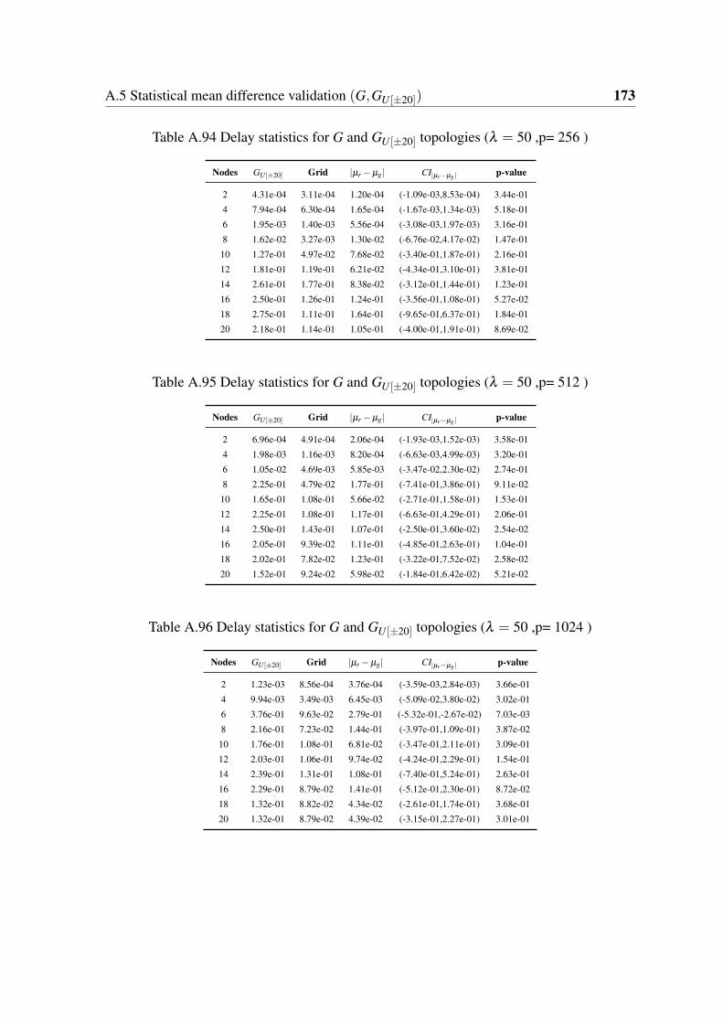
A.5 Statistical mean difference validation (G,GU [±20]) 173
Table A.94 Delay statistics for G and GU [±20] topologies (λ = 50 ,p= 256 )
Nodes GU [±20] Grid |µr−µg| CI|µr−µg | p-value
2 4.31e-04 3.11e-04 1.20e-04 (-1.09e-03,8.53e-04) 3.44e-01
4 7.94e-04 6.30e-04 1.65e-04 (-1.67e-03,1.34e-03) 5.18e-01
6 1.95e-03 1.40e-03 5.56e-04 (-3.08e-03,1.97e-03) 3.16e-01
8 1.62e-02 3.27e-03 1.30e-02 (-6.76e-02,4.17e-02) 1.47e-01
10 1.27e-01 4.97e-02 7.68e-02 (-3.40e-01,1.87e-01) 2.16e-01
12 1.81e-01 1.19e-01 6.21e-02 (-4.34e-01,3.10e-01) 3.81e-01
14 2.61e-01 1.77e-01 8.38e-02 (-3.12e-01,1.44e-01) 1.23e-01
16 2.50e-01 1.26e-01 1.24e-01 (-3.56e-01,1.08e-01) 5.27e-02
18 2.75e-01 1.11e-01 1.64e-01 (-9.65e-01,6.37e-01) 1.84e-01
20 2.18e-01 1.14e-01 1.05e-01 (-4.00e-01,1.91e-01) 8.69e-02
Table A.95 Delay statistics for G and GU [±20] topologies (λ = 50 ,p= 512 )
Nodes GU [±20] Grid |µr−µg| CI|µr−µg | p-value
2 6.96e-04 4.91e-04 2.06e-04 (-1.93e-03,1.52e-03) 3.58e-01
4 1.98e-03 1.16e-03 8.20e-04 (-6.63e-03,4.99e-03) 3.20e-01
6 1.05e-02 4.69e-03 5.85e-03 (-3.47e-02,2.30e-02) 2.74e-01
8 2.25e-01 4.79e-02 1.77e-01 (-7.41e-01,3.86e-01) 9.11e-02
10 1.65e-01 1.08e-01 5.66e-02 (-2.71e-01,1.58e-01) 1.53e-01
12 2.25e-01 1.08e-01 1.17e-01 (-6.63e-01,4.29e-01) 2.06e-01
14 2.50e-01 1.43e-01 1.07e-01 (-2.50e-01,3.60e-02) 2.54e-02
16 2.05e-01 9.39e-02 1.11e-01 (-4.85e-01,2.63e-01) 1.04e-01
18 2.02e-01 7.82e-02 1.23e-01 (-3.22e-01,7.52e-02) 2.58e-02
20 1.52e-01 9.24e-02 5.98e-02 (-1.84e-01,6.42e-02) 5.21e-02
Table A.96 Delay statistics for G and GU [±20] topologies (λ = 50 ,p= 1024 )
Nodes GU [±20] Grid |µr−µg| CI|µr−µg | p-value
2 1.23e-03 8.56e-04 3.76e-04 (-3.59e-03,2.84e-03) 3.66e-01
4 9.94e-03 3.49e-03 6.45e-03 (-5.09e-02,3.80e-02) 3.02e-01
6 3.76e-01 9.63e-02 2.79e-01 (-5.32e-01,-2.67e-02) 7.03e-03
8 2.16e-01 7.23e-02 1.44e-01 (-3.97e-01,1.09e-01) 3.87e-02
10 1.76e-01 1.08e-01 6.81e-02 (-3.47e-01,2.11e-01) 3.09e-01
12 2.03e-01 1.06e-01 9.74e-02 (-4.24e-01,2.29e-01) 1.54e-01
14 2.39e-01 1.31e-01 1.08e-01 (-7.40e-01,5.24e-01) 2.63e-01
16 2.29e-01 8.79e-02 1.41e-01 (-5.12e-01,2.30e-01) 8.72e-02
18 1.32e-01 8.82e-02 4.34e-02 (-2.61e-01,1.74e-01) 3.68e-01
20 1.32e-01 8.79e-02 4.39e-02 (-3.15e-01,2.27e-01) 3.01e-01

174 Statistical validation tables
Table A.97 Delay statistics for G and GU [±20] topologies (λ = 100 ,p= 256 )
Nodes GU [±20] Grid |µr−µg| CI|µr−µg | p-value
2 4.31e-04 3.11e-04 1.21e-04 (-1.10e-03,8.55e-04) 3.45e-01
4 1.36e-03 8.25e-04 5.39e-04 (-4.77e-03,3.70e-03) 3.64e-01
6 4.55e-02 5.37e-03 4.01e-02 (-3.33e-01,2.52e-01) 3.10e-01
8 4.84e-01 2.93e-01 1.90e-01 (-9.45e-01,5.65e-01) 3.05e-01
10 2.50e-01 3.42e-01 9.22e-02 (-6.19e-01,8.04e-01) 3.89e-01
12 3.09e-01 2.92e-01 1.74e-02 (-2.82e-01,2.48e-01) 5.92e-01
14 3.96e-01 3.13e-01 8.24e-02 (-4.44e-01,2.79e-01) 3.43e-01
16 3.25e-01 1.81e-01 1.44e-01 (-8.13e-01,5.25e-01) 2.03e-01
18 3.64e-01 1.53e-01 2.12e-01 (-3.74e-01,-4.92e-02) 3.89e-03
20 2.95e-01 2.14e-01 8.07e-02 (-3.89e-01,2.28e-01) 2.51e-01
Table A.98 Delay statistics for G and GU [±20] topologies (λ = 100 ,p= 512 )
Nodes GU [±20] Grid |µr−µg| CI|µr−µg | p-value
2 6.98e-04 4.91e-04 2.06e-04 (-1.93e-03,1.52e-03) 3.58e-01
4 9.44e-03 2.33e-03 7.11e-03 (-5.16e-02,3.74e-02) 2.57e-01
6 3.87e-01 2.74e-01 1.14e-01 (-8.95e-01,6.68e-01) 4.55e-01
8 3.84e-01 2.13e-01 1.71e-01 (-4.84e-01,1.42e-01) 4.26e-02
10 2.92e-01 2.54e-01 3.78e-02 (-1.41e-01,6.50e-02) 1.64e-01
12 2.49e-01 1.78e-01 7.11e-02 (-3.08e-01,1.66e-01) 2.06e-01
14 3.00e-01 2.21e-01 7.85e-02 (-3.75e-01,2.18e-01) 2.73e-01
16 2.83e-01 1.53e-01 1.30e-01 (-4.92e-01,2.32e-01) 1.20e-01
18 1.84e-01 9.29e-02 9.07e-02 (-1.69e-01,-1.25e-02) 6.03e-03
20 1.72e-01 1.07e-01 6.49e-02 (-5.15e-01,3.85e-01) 2.92e-01
Table A.99 Delay statistics for G and GU [±20] topologies (λ = 100 ,p= 1024 )
Nodes GU [±20] Grid |µr−µg| CI|µr−µg | p-value
2 1.24e-03 8.60e-04 3.80e-04 (-3.62e-03,2.86e-03) 3.65e-01
4 3.88e-01 1.73e-01 2.15e-01 (-1.27e+00,8.42e-01) 2.78e-01
6 4.23e-01 2.72e-01 1.51e-01 (-4.61e-01,1.59e-01) 8.86e-02
8 2.99e-01 1.63e-01 1.36e-01 (-3.65e-01,9.40e-02) 5.20e-02
10 3.24e-01 1.50e-01 1.75e-01 (-4.26e-01,7.69e-02) 3.15e-02
12 2.59e-01 1.41e-01 1.18e-01 (-2.84e-01,4.90e-02) 2.02e-02
14 2.85e-01 1.80e-01 1.05e-01 (-4.27e-01,2.17e-01) 2.04e-01
16 1.72e-01 1.30e-01 4.26e-02 (-3.22e-01,2.37e-01) 4.88e-01
18 1.31e-01 9.29e-02 3.85e-02 (-3.52e-01,2.75e-01) 4.86e-01
20 1.92e-01 9.49e-02 9.67e-02 (-4.31e-01,2.37e-01) 1.37e-01

A.5 Statistical mean difference validation (G,GU [±20]) 175
Table A.100 Delay statistics for G and GU [±20] topologies (λ = 200 ,p= 256 )
Nodes GU [±20] Grid |µr−µg| CI|µr−µg | p-value
2 4.33e-04 3.12e-04 1.21e-04 (-1.10e-03,8.59e-04) 3.45e-01
4 6.03e-02 2.25e-03 5.80e-02 (-5.29e-01,4.12e-01) 3.46e-01
6 4.86e-01 3.11e-01 1.74e-01 (-5.15e-01,1.67e-01) 7.78e-02
8 3.69e-01 2.81e-01 8.87e-02 (-2.54e-01,7.70e-02) 5.98e-02
10 2.75e-01 2.85e-01 9.19e-03 (-2.54e-01,2.73e-01) 8.65e-01
12 3.63e-01 2.58e-01 1.05e-01 (-3.25e-01,1.15e-01) 7.83e-02
14 2.95e-01 2.97e-01 2.48e-03 (-3.39e-01,3.44e-01) 9.75e-01
16 2.91e-01 2.55e-01 3.66e-02 (-6.57e-01,5.83e-01) 7.26e-01
18 2.70e-01 1.75e-01 9.47e-02 (-2.83e-01,9.40e-02) 5.96e-02
20 2.29e-01 1.95e-01 3.40e-02 (-1.38e-01,6.95e-02) 1.95e-01
Table A.101 Delay statistics for G and GU [±20] topologies (λ = 200 ,p= 512 )
Nodes GU [±20] Grid |µr−µg| CI|µr−µg | p-value
2 7.04e-04 4.94e-04 2.10e-04 (-1.96e-03,1.54e-03) 3.57e-01
4 3.09e-01 1.79e-01 1.30e-01 (-9.66e-01,7.05e-01) 5.10e-01
6 4.27e-01 2.77e-01 1.50e-01 (-5.65e-01,2.65e-01) 1.48e-01
8 3.24e-01 1.85e-01 1.39e-01 (-5.55e-01,2.77e-01) 1.78e-01
10 2.19e-01 1.85e-01 3.47e-02 (-2.19e-01,1.50e-01) 4.13e-01
12 2.15e-01 1.53e-01 6.26e-02 (-3.83e-01,2.57e-01) 2.86e-01
14 2.39e-01 2.20e-01 1.92e-02 (-3.26e-01,2.88e-01) 7.87e-01
16 2.20e-01 2.00e-01 2.00e-02 (-2.02e-01,1.62e-01) 6.34e-01
18 1.79e-01 1.40e-01 3.88e-02 (-3.27e-01,2.50e-01) 5.46e-01
20 1.97e-01 1.84e-01 1.25e-02 (-3.35e-01,3.10e-01) 8.26e-01
Table A.102 Delay statistics for G and GU [±20] topologies (λ = 200 ,p= 1024 )
Nodes GU [±20] Grid |µr−µg| CI|µr−µg | p-value
2 1.29e-03 8.74e-04 4.15e-04 (-3.88e-03,3.05e-03) 3.57e-01
4 2.00e-01 1.64e-01 3.61e-02 (-3.60e-01,2.88e-01) 6.28e-01
6 3.38e-01 2.20e-01 1.18e-01 (-6.24e-01,3.88e-01) 3.04e-01
8 2.89e-01 1.14e-01 1.75e-01 (-8.77e-01,5.27e-01) 1.44e-01
10 1.66e-01 1.46e-01 2.07e-02 (-2.53e-01,2.12e-01) 6.95e-01
12 3.50e-01 2.25e-01 1.25e-01 (-5.83e-01,3.34e-01) 2.78e-01
14 3.10e-01 1.19e-01 1.91e-01 (-6.93e-01,3.12e-01) 9.67e-02
16 1.50e-01 1.39e-01 1.11e-02 (-2.82e-01,2.60e-01) 8.48e-01
18 1.81e-01 1.24e-01 5.67e-02 (-4.65e-01,3.52e-01) 5.55e-01
20 2.52e-01 1.28e-01 1.24e-01 (-1.77e+00,1.52e+00) 5.50e-01

176 Statistical validation tables
Table A.103 Jitter statistics for G and GU [±20] topologies (λ = 10 ,p= 256 )
Nodes GU [±20] Grid |µr−µg| CI|µr−µg | p-value
2 1.41e-05 5.12e-05 3.71e-05 (-6.61e-05,1.40e-04) 7.08e-02
4 4.85e-04 4.19e-04 6.61e-05 (-1.13e-03,1.00e-03) 6.20e-01
6 9.97e-04 1.03e-03 3.08e-05 (-1.47e-03,1.53e-03) 8.80e-01
8 1.88e-03 1.41e-03 4.66e-04 (-1.58e-03,6.51e-04) 6.58e-02
10 2.62e-03 2.46e-03 1.61e-04 (-1.88e-03,1.56e-03) 4.80e-01
12 5.74e-03 4.32e-03 1.43e-03 (-8.38e-03,5.52e-03) 3.88e-01
14 5.48e-03 6.66e-03 1.18e-03 (-2.92e-03,5.27e-03) 2.36e-01
16 9.58e-03 6.60e-03 2.98e-03 (-1.33e-02,7.35e-03) 1.89e-01
18 1.14e-02 8.66e-03 2.79e-03 (-2.36e-02,1.81e-02) 3.62e-01
20 1.83e-02 1.34e-02 4.87e-03 (-1.88e-02,9.07e-03) 1.83e-01
Table A.104 Jitter statistics for G and GU [±20] topologies (λ = 10 ,p= 512 )
Nodes GU [±20] Grid |µr−µg| CI|µr−µg | p-value
2 3.19e-05 9.28e-05 6.09e-05 (-3.08e-05,1.53e-04) 2.51e-02
4 1.03e-03 7.36e-04 2.95e-04 (-2.67e-03,2.08e-03) 3.51e-01
6 1.99e-03 1.59e-03 4.01e-04 (-2.10e-03,1.30e-03) 3.16e-01
8 3.89e-03 2.62e-03 1.27e-03 (-4.27e-03,1.74e-03) 5.69e-02
10 5.21e-03 5.64e-03 4.29e-04 (-1.28e-02,1.37e-02) 8.27e-01
12 1.17e-02 1.13e-02 3.76e-04 (-1.84e-02,1.77e-02) 9.23e-01
14 1.10e-02 1.11e-02 1.20e-04 (-6.36e-03,6.60e-03) 9.33e-01
16 2.62e-02 1.37e-02 1.25e-02 (-9.10e-02,6.61e-02) 2.74e-01
18 4.19e-02 1.67e-02 2.52e-02 (-9.50e-02,4.47e-02) 7.76e-02
20 6.81e-02 3.61e-02 3.20e-02 (-1.71e-01,1.07e-01) 1.82e-01
Table A.105 Jitter statistics for G and GU [±20] topologies (λ = 10 ,p= 1024 )
Nodes GU [±20] Grid |µr−µg| CI|µr−µg | p-value
2 4.99e-05 2.05e-04 1.55e-04 (-1.34e-04,4.45e-04) 3.43e-02
4 2.31e-03 1.70e-03 6.18e-04 (-6.64e-03,5.40e-03) 4.20e-01
6 4.58e-03 4.07e-03 5.10e-04 (-3.20e-03,2.18e-03) 4.06e-01
8 1.03e-02 6.28e-03 4.05e-03 (-1.60e-02,7.91e-03) 1.16e-01
10 1.18e-02 1.15e-02 3.02e-04 (-2.51e-02,2.45e-02) 9.30e-01
12 4.82e-02 2.75e-02 2.07e-02 (-8.89e-02,4.75e-02) 2.35e-01
14 1.13e-01 3.89e-02 7.46e-02 (-3.48e-01,1.99e-01) 1.17e-01
16 9.04e-02 5.35e-02 3.69e-02 (-2.43e-01,1.70e-01) 2.40e-01
18 1.37e-01 6.57e-02 7.11e-02 (-4.92e-01,3.50e-01) 2.42e-01
20 1.30e-01 7.26e-02 5.69e-02 (-1.85e-01,7.09e-02) 7.94e-02
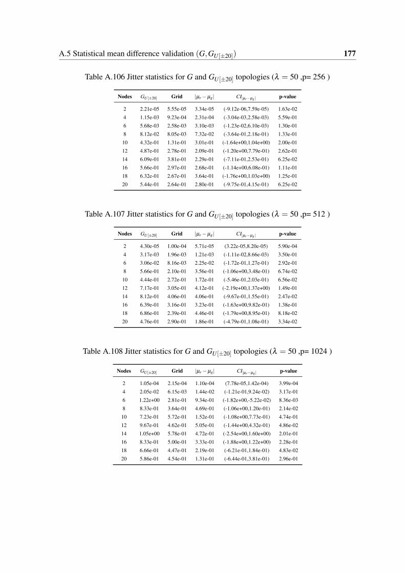
A.5 Statistical mean difference validation (G,GU [±20]) 177
Table A.106 Jitter statistics for G and GU [±20] topologies (λ = 50 ,p= 256 )
Nodes GU [±20] Grid |µr−µg| CI|µr−µg | p-value
2 2.21e-05 5.55e-05 3.34e-05 (-9.12e-06,7.59e-05) 1.63e-02
4 1.15e-03 9.23e-04 2.31e-04 (-3.04e-03,2.58e-03) 5.59e-01
6 5.68e-03 2.58e-03 3.10e-03 (-1.23e-02,6.10e-03) 1.30e-01
8 8.12e-02 8.05e-03 7.32e-02 (-3.64e-01,2.18e-01) 1.33e-01
10 4.32e-01 1.31e-01 3.01e-01 (-1.64e+00,1.04e+00) 2.00e-01
12 4.87e-01 2.78e-01 2.09e-01 (-1.20e+00,7.79e-01) 2.62e-01
14 6.09e-01 3.81e-01 2.29e-01 (-7.11e-01,2.53e-01) 6.25e-02
16 5.66e-01 2.97e-01 2.68e-01 (-1.14e+00,6.08e-01) 1.11e-01
18 6.32e-01 2.67e-01 3.64e-01 (-1.76e+00,1.03e+00) 1.25e-01
20 5.44e-01 2.64e-01 2.80e-01 (-9.75e-01,4.15e-01) 6.25e-02
Table A.107 Jitter statistics for G and GU [±20] topologies (λ = 50 ,p= 512 )
Nodes GU [±20] Grid |µr−µg| CI|µr−µg | p-value
2 4.30e-05 1.00e-04 5.71e-05 (3.22e-05,8.20e-05) 5.90e-04
4 3.17e-03 1.96e-03 1.21e-03 (-1.11e-02,8.66e-03) 3.50e-01
6 3.06e-02 8.16e-03 2.25e-02 (-1.72e-01,1.27e-01) 2.92e-01
8 5.66e-01 2.10e-01 3.56e-01 (-1.06e+00,3.48e-01) 6.74e-02
10 4.44e-01 2.72e-01 1.72e-01 (-5.46e-01,2.03e-01) 6.56e-02
12 7.17e-01 3.05e-01 4.12e-01 (-2.19e+00,1.37e+00) 1.49e-01
14 8.12e-01 4.06e-01 4.06e-01 (-9.67e-01,1.55e-01) 2.47e-02
16 6.39e-01 3.16e-01 3.23e-01 (-1.63e+00,9.82e-01) 1.38e-01
18 6.86e-01 2.39e-01 4.46e-01 (-1.79e+00,8.95e-01) 8.18e-02
20 4.76e-01 2.90e-01 1.86e-01 (-4.79e-01,1.08e-01) 3.34e-02
Table A.108 Jitter statistics for G and GU [±20] topologies (λ = 50 ,p= 1024 )
Nodes GU [±20] Grid |µr−µg| CI|µr−µg | p-value
2 1.05e-04 2.15e-04 1.10e-04 (7.78e-05,1.42e-04) 3.99e-04
4 2.05e-02 6.15e-03 1.44e-02 (-1.21e-01,9.24e-02) 3.17e-01
6 1.22e+00 2.81e-01 9.34e-01 (-1.82e+00,-5.22e-02) 8.36e-03
8 8.33e-01 3.64e-01 4.69e-01 (-1.06e+00,1.20e-01) 2.14e-02
10 7.23e-01 5.72e-01 1.52e-01 (-1.08e+00,7.73e-01) 4.74e-01
12 9.67e-01 4.62e-01 5.05e-01 (-1.44e+00,4.32e-01) 4.86e-02
14 1.05e+00 5.78e-01 4.72e-01 (-2.54e+00,1.60e+00) 2.01e-01
16 8.33e-01 5.00e-01 3.33e-01 (-1.88e+00,1.22e+00) 2.28e-01
18 6.66e-01 4.47e-01 2.19e-01 (-6.21e-01,1.84e-01) 4.83e-02
20 5.86e-01 4.54e-01 1.31e-01 (-6.44e-01,3.81e-01) 2.96e-01

178 Statistical validation tables
Table A.109 Jitter statistics for G and GU [±20] topologies (λ = 100 ,p= 256 )
Nodes GU [±20] Grid |µr−µg| CI|µr−µg| p-value
2 3.06e-05 5.82e-05 2.76e-05 (2.09e-05,3.42e-05) 4.67e-05
4 2.45e-03 1.50e-03 9.43e-04 (-9.36e-03,7.47e-03) 3.84e-01
6 1.18e-01 1.30e-02 1.05e-01 (-8.20e-01,6.10e-01) 2.84e-01
8 1.03e+00 6.31e-01 3.95e-01 (-2.21e+00,1.42e+00) 1.78e-01
10 7.20e-01 8.51e-01 1.31e-01 (-5.58e-01,8.20e-01) 3.85e-01
12 9.14e-01 7.67e-01 1.47e-01 (-6.58e-01,3.64e-01) 1.57e-01
14 1.04e+00 7.81e-01 2.63e-01 (-6.70e-01,1.44e-01) 4.07e-02
16 8.84e-01 5.86e-01 2.98e-01 (-1.85e+00,1.25e+00) 2.27e-01
18 9.91e-01 4.79e-01 5.11e-01 (-9.42e-01,-8.04e-02) 6.58e-03
20 8.11e-01 6.01e-01 2.10e-01 (-8.79e-01,4.58e-01) 1.87e-01
Table A.110 Jitter statistics for G and GU [±20] topologies (λ = 100 ,p= 512 )
Nodes GU [±20] Grid |µr−µg| CI|µr−µg| p-value
2 6.96e-05 1.07e-04 3.73e-05 (-4.19e-05,1.17e-04) 4.29e-02
4 2.36e-02 4.49e-03 1.91e-02 (-1.52e-01,1.13e-01) 2.89e-01
6 1.06e+00 7.82e-01 2.82e-01 (-3.08e+00,2.51e+00) 4.49e-01
8 1.15e+00 7.54e-01 3.95e-01 (-5.79e-01,-2.11e-01) 1.01e-03
10 9.70e-01 9.89e-01 1.85e-02 (-7.85e-01,8.22e-01) 8.47e-01
12 9.88e-01 6.85e-01 3.03e-01 (-9.62e-01,3.56e-01) 7.29e-02
14 1.19e+00 8.53e-01 3.40e-01 (-1.20e+00,5.19e-01) 8.14e-02
16 1.04e+00 6.02e-01 4.42e-01 (-1.42e+00,5.35e-01) 7.93e-02
18 7.62e-01 4.89e-01 2.73e-01 (-5.89e-01,4.34e-02) 1.61e-02
20 6.84e-01 5.21e-01 1.63e-01 (-9.36e-01,6.10e-01) 3.14e-01
Table A.111 Jitter statistics for G and GU [±20] topologies (λ = 100 ,p= 1024 )
Nodes GU [±20] Grid |µr−µg| CI|µr−µg | p-value
2 1.81e-04 2.35e-04 5.43e-05 (-3.01e-04,4.10e-04) 2.69e-01
4 1.31e+00 4.52e-01 8.60e-01 (-3.87e+00,2.14e+00) 1.22e-01
6 1.26e+00 1.13e+00 1.35e-01 (-6.59e-01,3.88e-01) 2.66e-01
8 1.17e+00 8.45e-01 3.27e-01 (-7.45e-01,9.22e-02) 2.26e-02
10 1.25e+00 8.16e-01 4.31e-01 (-1.32e+00,4.59e-01) 7.19e-02
12 1.18e+00 6.70e-01 5.08e-01 (-8.06e-01,-2.10e-01) 1.99e-03
14 1.21e+00 7.23e-01 4.86e-01 (-1.28e+00,3.07e-01) 4.75e-02
16 8.58e-01 6.30e-01 2.27e-01 (-1.05e+00,5.96e-01) 2.42e-01
18 7.30e-01 4.64e-01 2.66e-01 (-1.01e+00,4.82e-01) 1.16e-01
20 7.49e-01 5.23e-01 2.26e-01 (-8.93e-01,4.42e-01) 1.32e-01
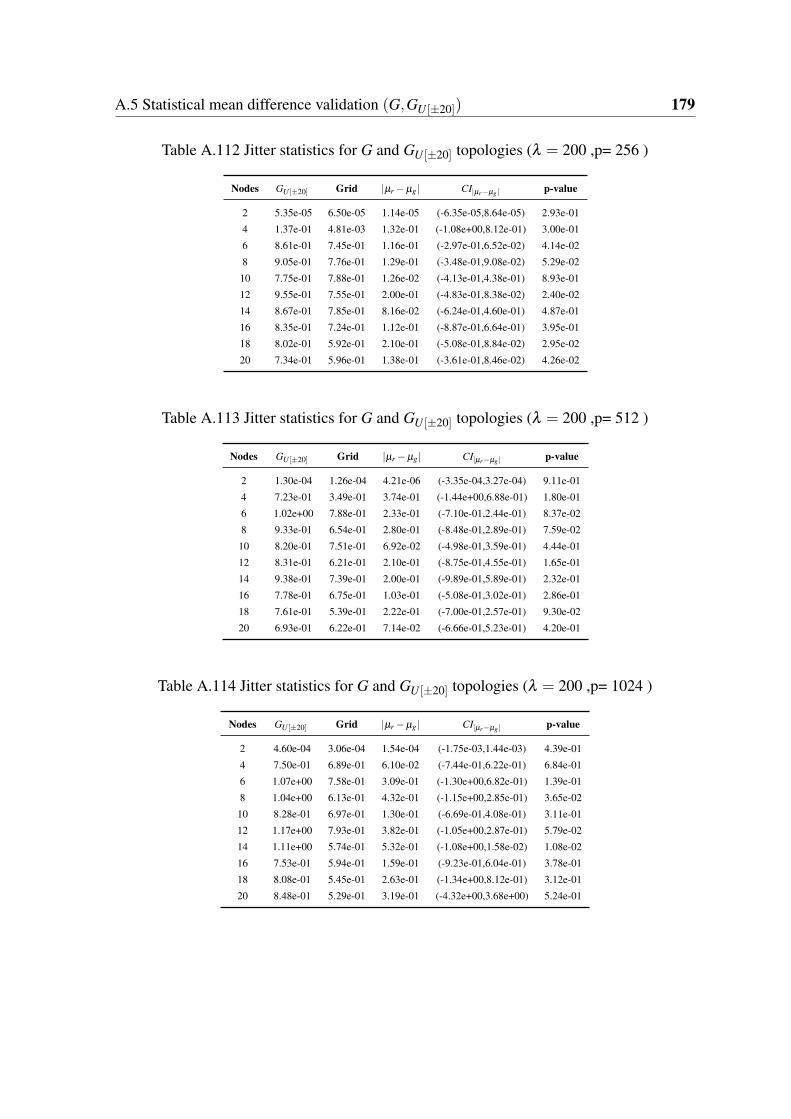
A.5 Statistical mean difference validation (G,GU [±20]) 179
Table A.112 Jitter statistics for G and GU [±20] topologies (λ = 200 ,p= 256 )
Nodes GU [±20] Grid |µr−µg| CI|µr−µg | p-value
2 5.35e-05 6.50e-05 1.14e-05 (-6.35e-05,8.64e-05) 2.93e-01
4 1.37e-01 4.81e-03 1.32e-01 (-1.08e+00,8.12e-01) 3.00e-01
6 8.61e-01 7.45e-01 1.16e-01 (-2.97e-01,6.52e-02) 4.14e-02
8 9.05e-01 7.76e-01 1.29e-01 (-3.48e-01,9.08e-02) 5.29e-02
10 7.75e-01 7.88e-01 1.26e-02 (-4.13e-01,4.38e-01) 8.93e-01
12 9.55e-01 7.55e-01 2.00e-01 (-4.83e-01,8.38e-02) 2.40e-02
14 8.67e-01 7.85e-01 8.16e-02 (-6.24e-01,4.60e-01) 4.87e-01
16 8.35e-01 7.24e-01 1.12e-01 (-8.87e-01,6.64e-01) 3.95e-01
18 8.02e-01 5.92e-01 2.10e-01 (-5.08e-01,8.84e-02) 2.95e-02
20 7.34e-01 5.96e-01 1.38e-01 (-3.61e-01,8.46e-02) 4.26e-02
Table A.113 Jitter statistics for G and GU [±20] topologies (λ = 200 ,p= 512 )
Nodes GU [±20] Grid |µr−µg| CI|µr−µg | p-value
2 1.30e-04 1.26e-04 4.21e-06 (-3.35e-04,3.27e-04) 9.11e-01
4 7.23e-01 3.49e-01 3.74e-01 (-1.44e+00,6.88e-01) 1.80e-01
6 1.02e+00 7.88e-01 2.33e-01 (-7.10e-01,2.44e-01) 8.37e-02
8 9.33e-01 6.54e-01 2.80e-01 (-8.48e-01,2.89e-01) 7.59e-02
10 8.20e-01 7.51e-01 6.92e-02 (-4.98e-01,3.59e-01) 4.44e-01
12 8.31e-01 6.21e-01 2.10e-01 (-8.75e-01,4.55e-01) 1.65e-01
14 9.38e-01 7.39e-01 2.00e-01 (-9.89e-01,5.89e-01) 2.32e-01
16 7.78e-01 6.75e-01 1.03e-01 (-5.08e-01,3.02e-01) 2.86e-01
18 7.61e-01 5.39e-01 2.22e-01 (-7.00e-01,2.57e-01) 9.30e-02
20 6.93e-01 6.22e-01 7.14e-02 (-6.66e-01,5.23e-01) 4.20e-01
Table A.114 Jitter statistics for G and GU [±20] topologies (λ = 200 ,p= 1024 )
Nodes GU [±20] Grid |µr−µg| CI|µr−µg | p-value
2 4.60e-04 3.06e-04 1.54e-04 (-1.75e-03,1.44e-03) 4.39e-01
4 7.50e-01 6.89e-01 6.10e-02 (-7.44e-01,6.22e-01) 6.84e-01
6 1.07e+00 7.58e-01 3.09e-01 (-1.30e+00,6.82e-01) 1.39e-01
8 1.04e+00 6.13e-01 4.32e-01 (-1.15e+00,2.85e-01) 3.65e-02
10 8.28e-01 6.97e-01 1.30e-01 (-6.69e-01,4.08e-01) 3.11e-01
12 1.17e+00 7.93e-01 3.82e-01 (-1.05e+00,2.87e-01) 5.79e-02
14 1.11e+00 5.74e-01 5.32e-01 (-1.08e+00,1.58e-02) 1.08e-02
16 7.53e-01 5.94e-01 1.59e-01 (-9.23e-01,6.04e-01) 3.78e-01
18 8.08e-01 5.45e-01 2.63e-01 (-1.34e+00,8.12e-01) 3.12e-01
20 8.48e-01 5.29e-01 3.19e-01 (-4.32e+00,3.68e+00) 5.24e-01

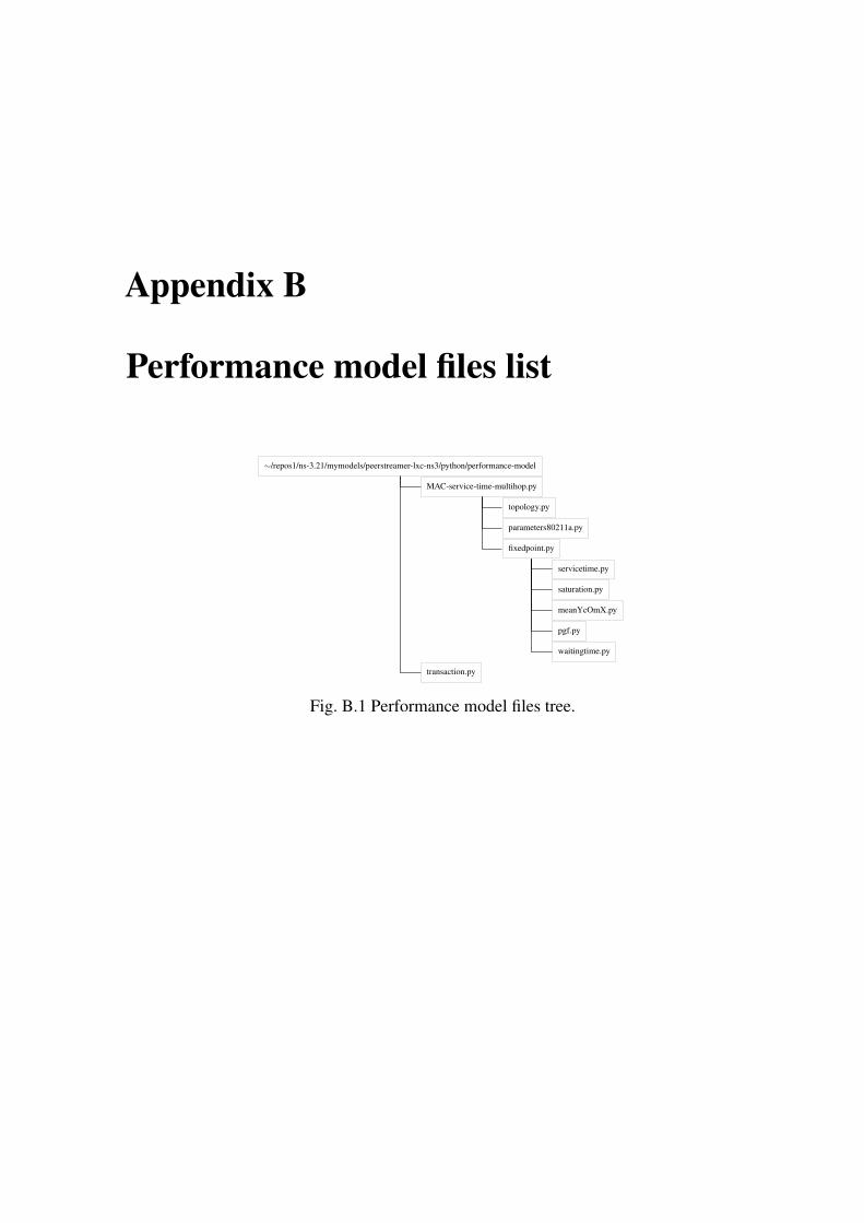
Appendix B
Performance model files list
∼/repos1/ns-3.21/mymodels/peerstreamer-lxc-ns3/python/performance-model
MAC-service-time-multihop.py
topology.py
parameters80211a.py
fixedpoint.py
servicetime.py
saturation.py
meanYcOmX.py
pgf.py
waitingtime.py
transaction.py
Fig. B.1 Performance model files tree.
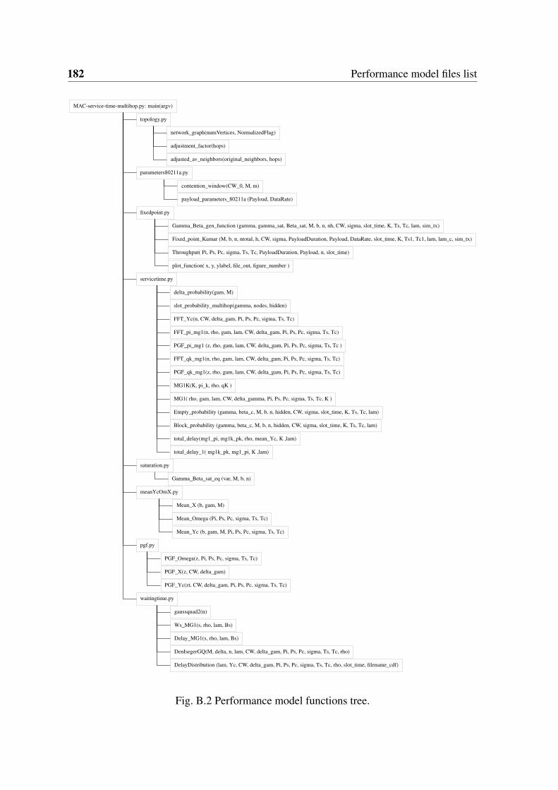
182 Performance model files list
MAC-service-time-multihop.py: main(argv)
topology.py
network_graph(numVertices, NormalizedFlag)
adjustment_factor(hops)
adjusted_av_neighbors(original_neighbors, hops)
parameters80211a.py
contention_window(CW_0, M, m)
payload_parameters_80211a (Payload, DataRate)
fixedpoint.py
Gamma_Beta_gen_function (gamma, gamma_sat, Beta_sat, M, b, n, nh, CW, sigma, slot_time, K, Ts, Tc, lam, sim_tx)
Fixed_point_Kumar (M, b, n, ntotal, h, CW, sigma, PayloadDuration, Payload, DataRate, slot_time, K, Ts1, Tc1, lam, lam_c, sim_tx)
Throughput( Pi, Ps, Pc, sigma, Ts, Tc, PayloadDuration, Payload, n, slot_time)
plot_function( x, y, ylabel, file_out, figure_number )
servicetime.py
delta_probability(gam, M)
slot_probability_multihop(gamma, nodes, hidden)
FFT_Yc(n, CW, delta_gam, Pi, Ps, Pc, sigma, Ts, Tc)
FFT_pi_mg1(n, rho, gam, lam, CW, delta_gam, Pi, Ps, Pc, sigma, Ts, Tc)
PGF_pi_mg1 (z, rho, gam, lam, CW, delta_gam, Pi, Ps, Pc, sigma, Ts, Tc )
FFT_qk_mg1(n, rho, gam, lam, CW, delta_gam, Pi, Ps, Pc, sigma, Ts, Tc)
PGF_qk_mg1(z, rho, gam, lam, CW, delta_gam, Pi, Ps, Pc, sigma, Ts, Tc)
MG1K(K, pi_k, rho, qK )
MG1( rho, gam, lam, CW, delta_gamma, Pi, Ps, Pc, sigma, Ts, Tc, K )
Empty_probability (gamma, beta_c, M, b, n, hidden, CW, sigma, slot_time, K, Ts, Tc, lam)
Block_probability (gamma, beta_c, M, b, n, hidden, CW, sigma, slot_time, K, Ts, Tc, lam)
total_delay(mg1_pi, mg1k_pk, rho, mean_Yc, K ,lam)
total_delay_1( mg1k_pk, mg1_pi, K ,lam)
saturation.py
Gamma_Beta_sat_eq (var, M, b, n)
meanYcOmX.py
Mean_X (b, gam, M)
Mean_Omega (Pi, Ps, Pc, sigma, Ts, Tc)
Mean_Yc (b, gam, M, Pi, Ps, Pc, sigma, Ts, Tc)
pgf.py
PGF_Omega(z, Pi, Ps, Pc, sigma, Ts, Tc)
PGF_X(z, CW, delta_gam)
PGF_Yc(zt, CW, delta_gam, Pi, Ps, Pc, sigma, Ts, Tc)
waitingtime.py
gaussquad2(n)
Ws_MG1(s, rho, lam, Bs)
Delay_MG1(s, rho, lam, Bs)
DenIsegerGQ(M, delta, n, lam, CW, delta_gam, Pi, Ps, Pc, sigma, Ts, Tc, rho)
DelayDistribution (lam, Yc, CW, delta_gam, Pi, Ps, Pc, sigma, Ts, Tc, rho, slot_time, filename_cdf)
Fig. B.2 Performance model functions tree.
Related Documents