Performance Evaluation for Adaptive Modulation Wireless ...

Performance Evaluation for Adaptive Modulation Wireless System over Rayleigh

Fading Channel Using Finite State Markov Chain (FSMC) Technique

by

Khamis Elnawaa

B.Sc., University of Benghazi, 2009

A Project Submitted in Partial Fulfillment of the

Requirements for the Degree of

MASTER OF ENGINEERING

in the Department of Electrical and Computer Engineering

c© Khamis Elnawaa, 2017

University of Victoria

All rights reserved. This project may not be reproduced in whole or in part, by

photocopying or other means, without the permission of the author.

ii

Performance Evaluation for Adaptive Modulation Wireless System over Rayleigh

Fading Channel Using Finite State Markov Chain (FSMC) Technique

by

Khamis Elnawaa

B.Sc., University of Benghazi, 2009

Supervisory Committee

Dr. Fayez Gebali, Supervisor

(Department of Electrical and Computer Engineering)

Dr. Mihai Sima, Departmental Member


iii

Supervisory Committee

Dr. Fayez Gebali, Supervisor


Dr. Mihai Sima, Departmental Member


ABSTRACT

In this project, adaptive modulation for end to end wireless link system using

MQAM modulation scheme over Rayleigh fading channel is addressed. Selecting

the modulation schemes, which maintain appropriate frame error rate and maximum

throughput, according to channel states is discussed. First order finite state Markov

chain (FSMC) model is utilized to model the channel states in terms of SNR. In

order to get the best choice modulation scheme selection for the adaptive modulation

system, a new method for channel partitioning the is proposed. In this method, we

select the SNR levels of the channel based on a desired (target) FER of the system

with respect to the average time of channel state duration. We present another

method for channel petitioning, which is called equilibrium steady state method.for

both methods, performance measures of the FSMC model for Rayleigh channel are

derived, plotted and analyzed. The performance analysis of the system and numerical

results of both methods are compared and discussed.

iv

Contents

Supervisory Committee ii

Abstract iii

Table of Contents iv

List of Tables vi

List of Figures vii

Acknowledgements ix

Dedication x

1 Introduction 1

1.1 Contributions . . . . . . . . . . . . . . . . . . . . . . . . . . . . . . . 2

1.2 Project Organization . . . . . . . . . . . . . . . . . . . . . . . . . . . 3

2 Overview of Channel Models and Adaptive Modulation Technique 4

2.1 Channel Models . . . . . . . . . . . . . . . . . . . . . . . . . . . . . 4

2.1.1 Statistical Fading Channel Models . . . . . . . . . . . . . . . 4

2.1.2 Pathloss and Shadowing . . . . . . . . . . . . . . . . . . . . . 4

2.1.3 Multipath Fading . . . . . . . . . . . . . . . . . . . . . . . . . 5

2.1.4 Frequency-Flat Fading . . . . . . . . . . . . . . . . . . . . . . 6

2.2 Performance Analysis over Fading Channels . . . . . . . . . . . . . . 7

2.3 Adaptive Modulation . . . . . . . . . . . . . . . . . . . . . . . . . . . 8

2.3.1 Constant-Power Variable-Rate Adaptive M-QAM . . . . . . . 8

2.3.2 Packet and Frame Structures . . . . . . . . . . . . . . . . . . 9

2.4 Performance Analysis of Adaptive Modulation System Model . . . . 11

2.4.1 Frame Error Rate . . . . . . . . . . . . . . . . . . . . . . . . 11

v

3 Overview of Finite State Markov Chain (FSMC) 13

3.1 Finite State Markov Chain (FSMC) for radio channel . . . . . . . . . 13

3.1.1 Finite State Markov Chain (FSMC) Model for Rayleigh Fading

Channel . . . . . . . . . . . . . . . . . . . . . . . . . . . . . . 14

3.1.2 Average Throughput Analysis Using FSMC’s Parameters . . . 16

4 Channel Partitioning Methods of FSMC 17

4.1 Signal to noise ratio partitioning . . . . . . . . . . . . . . . . . . . . . 17

4.1.1 Steady State Equilibrium Method . . . . . . . . . . . . . . . 17

4.1.2 Error Rate Curve Partitioning Method . . . . . . . . . . . . . 18

4.1.3 Relationship between Average Time Duration of a State and

SNR Thresholds of the Same State . . . . . . . . . . . . . . . 20

5 System Setup and Results Discussion 23

5.1 Model of End to End Adaptive Modulation System . . . . . . . . . . 23

5.1.1 System Model Assumptions . . . . . . . . . . . . . . . . . . . 24

5.2 Results of Steady State Equilibrium Partitioning Method . . . . . . . 25

30

6 Conclusion 37

vi

List of Tables

Table 2.1 State Dependent Parameters of FERM(γ) Equation. . . . . . . . 12

Table 4.1 Constant ck and Γi thresholds values calculation based on equal

step size ∆n for all states. . . . . . . . . . . . . . . . . . . . . . 21

Table 4.2 Constant ck and Γi thresholds values calculation based on non-

equal step size ∆n for all states. . . . . . . . . . . . . . . . . . . 21

Table 5.1 Values of channel thresholds and the adaptive modulation thresh-

olds at target FER = 10−3 calculated using steady state equilib-

rium partitioning method. . . . . . . . . . . . . . . . . . . . . . 30


olds at target FER = 10−3 calculated using error rate curve par-

titioning method. . . . . . . . . . . . . . . . . . . . . . . . . . 35


olds at target FER = 10−6 calculated using error rate curve par-

titioning method. . . . . . . . . . . . . . . . . . . . . . . . . . . 35

vii

List of Figures

Figure 2.1 The packet and the frame structures [17]. . . . . . . . . . . . . 10

Figure 2.2 Theoretical FER curve and FER fitted curve of M-QAM adaptive

modulation modes over Rayleigh fading channel. . . . . . . . . 12

Figure 3.1 FSMC model illustrated the state transitions probabilities for k

number of states . . . . . . . . . . . . . . . . . . . . . . . . . . 16

Figure 4.1 The FER verses SNR curves for adaptive transmission system,

uses three different M-QAM modulation schemes. . . . . . . . . 18

Figure 4.2 The relationship between constant ck and thresholds Γi with

equal step size (∆n) for all states. . . . . . . . . . . . . . . . . 22

Figure 4.3 The relationship between constant ck and thresholds Γi with non-

equal step size (∆n) for all states. . . . . . . . . . . . . . . . . 22

Figure 5.1 End to End wireless link system model. . . . . . . . . . . . . . 24

Figure 5.2 Steady state probabilities verses state index for Rayleigh fading

channel using steady state equilibrium partitioning method. . . 26

Figure 5.3 Number of crossing rate verses state index for Rayleigh fading

channel using steady state equilibrium partitioning method. . . 27

Figure 5.4 The transition probabilities for Rayleigh fading channel using

steady state equilibrium partitioning method. . . . . . . . . . . 28

Figure 5.5 Average frame error rate per mode verses state index for the

steady state equilibrium partitioning method. . . . . . . . . . . 29

Figure 5.6 Average throughput per state in bits of each mode in case target

FER = 10−3 for the steady state equilibrium partitioning method. 29

Figure 5.7 Steady state probabilities verses states in case target FER= 10−3

using error rate curve partitioning method. . . . . . . . . . . . 31

Figure 5.8 Number of crossing rate verses states in case target FER= 10−3

using error rate curve partitioning method. . . . . . . . . . . . 32

viii

Figure 5.9 The transition probabilities for Rayleigh fading channel in case

FER = 10−3 using error rate curve partitioning method. . . . . 33

Figure 5.10Average frame error rate per mode verses state index in case

target FER= 10−3 using error rate curve partitioning method . 34

Figure 5.11Average frame error rate per mode verses state index in case

target FER= 10−6 using error rate curve partitioning method . 34

Figure 5.12Average Throughput per state in bits of each mode in case target

FER= 10−3 using error rate curve partitioning method . . . . . 36

Figure 5.13Average throughput per state in bits of each mode in case target

FER= 10−6 using error rate curve partitioning method. . . . . 36

ix

ACKNOWLEDGEMENTS

I would like to thank:

my father, mother, and my wife, for supporting me in the low moments.

Dr.Fayez Gebali, for mentoring, support, encouragement, and patience.

the Ministry of Education of Libya , for funding me with a Scholarship.

In The Name of Allah, The Beneficent, The Merciful. “Read In the Name of your

Lord Who created.” “Created man, out of a clot.” “Read, and your Lord is the Most

Generous.” “Who taught by the Pen.” “Taught man that which he knew not.”

Quran Book, Surah ‘Alaq, Chapter 96

x

DEDICATION

To my mother, Khouloud Gatan and my father, Hamid Elnawaa and my wife,

khadeejah Hamzah, they were the secret of my diligence. It would not be

possible without their support.

To my supervisor, Dr. Fayez Gebali, he is always supportive and helpful. I

appreciate his invaluable time he spent with me for his supervision.

Chapter 1

Introduction

The use of wireless communication networks in multimedia makes the need for high

data rates grow rapidly. Providing a high data rate in networks is challenging due to

several issues. For instance, Bottleneck phenomenon that occurs in wireless links, is

one of the challenged problems. The cause of the Bottleneck phenomenon is not only

because of wireless resources such as bandwidth availability and power expensive, but

also because of Doppler frequency, multipath fading, and wireless propagation that

degrades the overall system performance. One of the ways to enhance performance of

the wireless link is called Adaptive transmission. This technique targets the enhance-

ment of the spectral efficiency of the network. In this technique, a target error rate

over wireless channel has to be chosen to ensure high performance of the network.

Adaptive transmission has been widely used to match transmission parameters to

time-varying channel conditions [1] [6] [11] [12] [18]. Due to the high performance of

the adaptive transmission technique, it has been connected to the physical layer of

several standards, e.g., IEEE 802.11a, IEEE 802.15.3, IEEE 802.16, and 3GPP [16]

[8] [9] [15].

In order to model wireless fading channels and to evaluate the performance of cer-

tain signal transmission techniques over wireless channels, finite state Markov chain

(FSMC) is widely used to describe the wireless fading channels behavior and to eval-

uate the performance of a particular system over different types of wireless fading

channels. In radio mobile communication, FSMC model was used to evaluate the per-

formance of the fading channels [24], where each set of Signal-to-Noise Ratio (SNRs)

was represented by a state in the FSMC. In [5], the order of fading channel memory

is explained in auto regressive modeling (AR) of time varying flat fading channel,

and that models help to describe the time variation of the fading channel gain accu-

2

rately. In [20] the authority and the accurateness of the FSMC as a model for the

Rayleigh fading channels is presented through the state balance equations. In [2], re-

ceived SNRs that have Lognormal, K and Chi-square distribution is represented using

FSMC model. The performance measurement and parameters such as steady state

probability, level crossing rate, and state transition probability are derived. In [19],

the first order FSMC model, which can be acquired for fading channels, is described.

The paper also discusses its applications.

In [14], the author presents a technique to calculate the parameters of FSMC

that matches a Nakagami-m distribution - slow fading channel. The author in [10]

presents a finite state Markov model of Nakagami fading to evaluate the performance

of adaptive coding transmission technique. The throughput analytical evaluation of

the adaptive coding is obtained. In [23], the author presents an analytical method

utilizing FSMC to implement an error model for performance estimation of adaptive

modulation system (AMS) combined with automatic repeat request (ARQ) shcemes

in slow fading channels.

1.1 Contributions

In adaptive modulation systems, selecting the modulation schemes, which maintain

appropriate frame error rate and maximum throughput according to the channel

state, is interesting problem. In order to select the modulation schemes of adaptive

modulation technique, and to investigate the complicity of mapping the received SNR

into FSMC channel’s thresholds to make the right decision of modulation switching as

in [23], a new method for FSMC channel portioning is proposed. This work includes

the following contributions:

1- The received SNR threshold of each mode of the adaptive modulation and

the average time duration τi are taken into account for FSMC channel partitioning

calculation

2- The relationship between the average time duration and the SNR thresholds is

theoretically plotted and discussed.

3

1.2 Project Organization

This section gives a brief remainder of this project . For each of the chapters below,

there is a short summary of what the project focus is.

Chapter 2 discusses statistical fading channel models and adaptive modulation tech-

nique.

Chapter 3, present Finite State Markov Chain FSMC model, and performance mea-

sures of the model such as state time duration, state transition probability,steady

state probability, and crossing rate are analyzed. These parameters are used to eval-

uate End-to-End system with adaptive modulation technique over Rayleigh fading

channel.

Chapter 4 presents the portioning methods of the channels and describes the rela-

tionship between the average time channel state duration and the SNR thresholds.

Chapter 5 presents the system model, and the assumptions that related to the chan-

nel environment are pointed out. Also ,FSMC model parameters are plotted, and the

performance evaluation results such as the average throughput and the average FER

of the system are discussed and plotted.

Chapter 6, presents the project conclusion.

4

Chapter 2

Overview of Channel Models and

Adaptive Modulation Technique

2.1 Channel Models

2.1.1 Statistical Fading Channel Models

The electromagnetic wave propagation affects the transmitted signal on wireless chan-

nels. The multiple propagation paths between the sender and the receiver appear

when radio waves propagate through several mechanisms such as scattering, reflec-

tion, diffraction, and LOS. Modeling of wireless channels is challenging since the

nature of the propagation is unpredictable, and the propagation environment is com-

plicated. Usually to characterize the wireless channels, there are three major effects

which have to be considered: path loss, shadowing, and fading. These effects will be

discussed briefly in the following sections.

2.1.2 Pathloss and Shadowing

Free space propagation (Pathloss) happens since the wave spreads over distance be-

tween the transmitter and the receiver; thus, power loss through the channel. The

Path loss has a large scale propagation effect because the variation in the signal occurs

over a large distance compared to the wavelength. Linear path loss is known as the

ratio between the power of the transmitted signal Pt over the power of the received

signal Pr, i.e. Pl = Pt/Pr. For high level system analysis, the log-distance model is

the most suitable model for this kind of analysis [21]. With regards to the log-normal

5

model, the path loss at distance d can be predicted by the following formula [21]:

Pl (d) db = Pl (d0) db + 10 γ log(d

d0

) (2.1)

where d0 is the reference distance, Pl(d0)db is the path loss at d0, and γ is the path

loss exponent.

Shadowing is a phenomenon that appears due to a large objects (building) presence

between the transmitter and the receiver and it has a large scale propagation effect.

These objects could attenuate the magnitude of the transmitted signal due to its

dielectric properties. Using the log-normal shadowing model, we could find the PDF

distribution of the received power by [21]:

p (x) =1

xσ√

2πexp[−(ln(x)− µ)2

2σ2] (2.2)

where x = Pt/Pr, σ is the standard deviation of x, and µ is the mean of x.

2.1.3 Multipath Fading

Multipath fading describes the impact of random overlap among arrived copies of

the original transmitted signal at the receiver. In other words, it characterizes the

effects of the received signal’s copies from different propagation paths on the desired

received signal. These signal’s copies generated from the fact that the transmitted

signal could be scattered, or reflected, depends on the channel environment. Fading

occurs in short distance compared to the signal wavelength, and is classified as a

small-scale phenomenon.

To write the formulation of the received signal over multipath fading, let us assume

s(t) is a signal transmitted over a wireless channel as follows [21]:

s (t) = Re[u(t)ej2πfct] (2.3)

where u(t) is complex baseband envelope. The received signal over the multipath

channel will be as follows [21]:

r (t) = Re

N(t)∑n=0

αn (t)u (t− τn (t)) ej2πfc(t−τn(t))+∅Dn(t)

(2.4)

where N(t) is the number of paths, αn (t) is the amplitude , τn (t) is the delay, and

6

∅Dn(t) is the phase shift, which is equal to∫

2πfDn (t) .dt , where fDn (t) is Doppler

frequency.

The multipath fading channel can be classified as frequency selective or flat fading.

Also it can be classified as fast or slow fading. These classifications are based on the

relative severity of the time-domain variation and power delay spread that cause the

transmitted signal over the wireless channel. Multipath channel introduces power

spared, and to quantify it along the delay axis, Root Mean Square (RMS) delay

spread (σT ) can be used. The RMS delay spread can be calculated as follows [21]:

σT =

√∑N0 αn

2(τn−µT )2∑Nn=0 αn

2(2.5)

where µT is the average delay spread, and it given as follows:

µT =

∑Nn=0 αn

2τn∑N0 αn

2(2.6)

If the symbol period of the transmitted signal is small compared to the delay

spread σT , then intersymbol interference (ISI) will occur, and the time-domain delay

spread will translate to selective frequency in frequency domain. If σT is very small

compared to the symbol time Ts, the wireless channel will be considered flat fading.

Otherwise the channel will be considered selective fading. We can convert frequency

selective channel into multiple parallel frequency-flat fading channels with the well-

known multicarrier transmission over OFDM technique. (Reference 2 in [21]).

2.1.4 Frequency-Flat Fading

The scenario where the delay spread is smaller than the transmit signal symbol period

i.e. σT � Ts reflects the flat fading phenomenon. The multipath signals can be

considered to reach the receiver side at the same time, and the complex baseband

input/output relationship of the channel is as in [21]:

r (t) = z (t)u (t) + n(t) (2.7)

where u(t) is the transmitted complex envelop, n(t) is the additive Gaussian noise,

and z(t) is equal to z(t)= zi (t) + jzq (t). Note, z(t) can be modeled as a Gaussian

random process with the application of central limit theorem (CLT) [21].

In the case where there is no LOS component, the random process z(t) has zero

7

mean, thus, the channel amplitude | z(t) |=√zi(t)

2 + zq(t)2 is Rayleigh distributed

with distribution function as follows [21]:

P|z| (x) =x

σ2exp[− x2

2σ2] (2.8)

where σ2 is the variance of z(t).

2.2 Performance Analysis over Fading Channels

The complex baseband channel model for flat fading is mentioned in equation (2.7).

The instantaneous power of the received signal can be shown as Pr = |z(t)|2Es/Tsand will be random variable with |z(t)|2 values. The instantaneous SNR is also shown

as γs = |z(t)|2Es/No.

The overall system performance can not be reflected by the instantaneous system

performance. Therefore, the average performance measures should be taken to reflect

the overall system performance. The average error rate can be calculated by averaging

the instantaneous error rate over the distribution of SNR. It is important to know

that at any time instant, the fading channel can be viewed as an AWGN channel

with SNR, γs = |z(t)|2Es/No, so over flat fading channel, the average error rate for

a certain modulation scheme can be calculated by averaging the instantaneous error

rate over the distribution function of γs. Theoretically, as in [21], the average error

rate is giving by:

PE =

∫ ∞0

PE(γ)pγ (γ) dγ (2.9)

where PE(γ) is the error rate over the AWGN channel with SNR and the distribution

is function of γ.

8

2.3 Adaptive Modulation

In a wireless link with fading channels, adaptive transmission can be utilized to

achieve high spectral and power efficiency with low error rate [21]. Basically, adaptive

transmission technique varies the transmission parameters and/or the transmission,

schemes such as modulation mode, coding rate, or transmission power, depend on in

current fading channel state. The system chooses the best channel condition to send

the data with high rate and low power level, and responds to channel degradation

to reduce data rate or increase power level. As a result, a certain desired error rate

will be reached, and thus overall system throughput will be maximized. As such, this

technique has recently seen growing interest in academia to meet the demands of high

transmission efficiency over fading channels. Now, adaptive transmission schemes are

incorporate in GSM/CDMA cellular systems and wireless LAN systems [21].

The fundamental requirement of adaptive transmission techniques is the availabil-

ity of certain channel state information (CSI) at the transmitter. With perfect CSI

at the transmitter, Shannon capacity can be reached over fading channels using op-

timal adaptive transmission scheme involving continuous rate and power adaptation.

However, the condition of perfect channel state at the transmitter is a challenging

task in reality even for recent advanced wireless systems. Also, continuous rate adap-

tation will be highly complex. As a result, most current wireless standards assume

adaptive transmission schemes employing discrete adaptation, which requires only

limited channel state information at the transmitter, achieved through feedback sig-

naling. The constant -power variable-rate adaptive M-QAM scheme is employed in

this work.

2.3.1 Constant-Power Variable-Rate Adaptive M-QAM

In the constant-power variable-rate adaptive M-QAM scheme, the system uses a fixed

power level for transmission. Assuming an adaptive M-QAM system uses a certain

power level, the system selects one of N dissimilar modulation schemes based on

channel conditions. Each modulation scheme has a different constellation size. The

constellation size for rectangular or squared M-QAM schemes is denoted by M , and

it is chosen to be M = 2n, n = 1,2,3,. . . , where n in bps/Hz. The modulation schemes

are chosen to reach the highest spectral value. The value range of the channel quality

is indicated by dividing the received SNR in to (N + 1) regions with threshold values

γt0 < γt1 < γt2 < . . . γt3 < γ∞.

9

When the received SNR falls into the nth region, i.e. tn≤ tn+1, the constellation

size (M) will be selected for transmission. In reality, the channel estimator estimates

the received SNR at the receiver, and the modulation mode selection chooses the

mode depending on the received SNR. The receiver feeds back the selected mode to

the transmitter over the control channels [21].

The thresholds are chosen under the condition that the instantaneous bit error

rate of the chosen modulation mode is below a certain target value, denoted by BER0.

For instance, as in reference [4], instantaneous bit error rate of square 2n- QAM with

two-dimensional Grey coding over AWGN channel with SNR can be calculated by:

BERn(γ) =2√

Mlog2

√M×

log2√M∑

k=1

(1−2−k)√M−1∑

i=0

(−1)

⌊ik−1√M

⌋(2k−1 −

⌊i2k−1

√M

+1

2

⌋)

×Q(

(2i+ 1)√

6log2M2(M−1)

γ)

(2.10)

As in reference [23], equation (2.10) can be approximated using a simple formula as

follows:

BERn(γ) =

{1 0 < γ < γpn

aMexp (−gMγ) γ ≥ γpn(2.11)

where n is the mode index, and, aM , gM , and γpn are state dependent parameters

which are obtained by fitting the curve of equation (2.11), to the exact curve BERn(γ)

of equation (2.10) by using least-mean-square method [17]. In the upcoming sections

the parameters aM , gM , and γpn are calculated to fit frames error rate curves. The

fitting graphs are shown too. For a target bit error rate (BER0) ,the threshold values

can be calculated as follows:

γTn = − 1

gMln

(BER0

aM

), n = 0, 1, 2, . . .,N. (2.12)

2.3.2 Packet and Frame Structures

Adaptive transmissions systems deal with frames in the physical layer. The signal

will be sent in term of frames. Each frame contains a fixed number of symbols

NF . Assuming the symbol rate is fixed, the frame duration time will be constant.

10

Having constant frame duration can be used to calculate the parameters of Markov

model for the channel model, as it shown in next sections. Each frame contains a

number of packets from the data layer, and each packet contains number of bits N b,

which include packet header, cyclic redundancy check, and payload. After modulation

and coding with rate Rm= (bits/symbol), each packet is mapped to a symbol block

containing N b/ Rm symbols. These blocks are used to build the frame, so the data

can be transmitted in the physical layer. The number of symbols per frame can be

calculated as follows [17]:

NF = Nc +NbNp/Rm (2.13)

where N c contains the pilot symbols and control part, and Np is the number of packets

per frame. The value of the number of packets per frame depends on the rate Rm of

the modulation and coding schemes. Also we can calculate the frame time duration

as follows [17]:

Tf = (N c +Np)/R (2.14)

where R is the rate in bits per second of the system. The packet and the frame

structures are shown in Figure 2.1.

Figure 2.1: The packet and the frame structures [17].

11

2.4 Performance Analysis of Adaptive Modulation

System Model

2.4.1 Frame Error Rate

Having the instantaneous bit error rate BERM(γ) of M-QAM modulation format

(2.10), we can calculate the exact-packet-error rate PERM(γ) as follows [23]:

PERM(γ) = 1− (1−BERM(γ))Nb (2.15)

where Nb is number of bits per packets. Having the exact packet error rate PERM(γ),

we also can calculate the frame error rate FERM(γ) as follows [23]:

FERM(γ) = 1− (1−BER2(γ))Nc(1− PERM(γ))

Np(M) (2.16)

where Nc is the total number of symbols in the header and in the control part. As in

[17] for the PERM(γ) approximation, we could also find FERM(γ) approximation as

follows [23]:

FERM(γ) =

{1 0 < γ < γpn

aM exp (−gM γ) γ ≥ γpn(2.17)

where M(γ) is the state index, and the state dependent parameters, aM ,gM , and

γpn are obtained by fitting the curve of equation (2.17), to the exact curve FERM(γ)

of equation (2.16) by using least-mean-square method [23]. The state dependent

parameters for different M-QAM modulation modes are calculated and they are shown

in Table 2.1.

In order to calculate adaptive modulation thresholds in terms of packet error rate

or in term of frame error rate, we can rewrite equation (2.12) to the follows:

γTn = − 1

gMln

(FER0

aM

), n = 0, 1, 2, . . ., N (2.18)

where FER0 is the desired or target frame error rate of a system . The curves in

Figure 2.2 display the FER fitting curve per mode calculated by equation (2.17), and

the exact FER per mode calculated by equation (2.16). these results are regenerated

and are matched the results in reference [23].

12

Table 2.1: State Dependent Parameters of FERM(γ) Equation.

Mode (M) Ratebit/symbol

aM gM γpn (db)

4-QAM 2 70.21 0.9929 7.5

8-QAM 3 87.98 0.4971 10.73

16-QAM 4 99.19 0.3948 11.76

32-QAM 5 106 0.1896 14.99

64-QAM 6 118.4 0.1417 16.399

Figure 2.2: Theoretical FER curve and FER fitted curve of M-QAM adaptive mod-ulation modes over Rayleigh fading channel.

In order to calculate average frame error rate for each mode of adaptive modulation

model over Rayleigh, The average frame error rate per mode can be calculated as

follows:

FERM =1

πM

∫ γt+1

γt

FERM(γ) pγ (γ) dγ (2.19)

where πM is the probability of being in the current mode ,and it will be shown in

next chapter.

13

Chapter 3

Overview of Finite State Markov

Chain (FSMC)

3.1 Finite State Markov Chain (FSMC) for radio

channel

Finite State Markov Chain protrudes from early the works of GIBERT and ELLIOTT.

Modeling the Radio channel as two states was not enough in order to form channel

variation; the solution to forming channel variation is to form the channel with more

than two stats. Let us assume vector s = {s0, s1, . . . sk−1} denote a finite set of states

in the channel and sn be a constant Markov process. sn is a constant which has the

property of stationary transition, so the transition probability between the states is

independent of the time index n and it can be written as in reference [20] as follows:

pj,k = Pr (sn+1 = sk/ sn = sj) (3.1)

where n = {0,1,2, . . . } , j and k are current and next states respectively (j,k) ∈ (0,

1,2,. . .K−1) , and K is number of states. With these definitions, we can calculate the

state transitions probability matrix P with elements pj,k as in (3.1). The probability

of staying in state k at any possible time index n is called stationary transition

property and it can be defined as follows:

πk = Pr( sn = sk), k ∈ {0, 1, 2, 3, . . . K − 1}. (3.2)

For a state k, the outcome and income flows must be equal. This assumption is called

14

equilibrium condition, and is shown as follows:

k−1∑j=0

πjpj,k =k−1∑i=0

πkpk,i (3.3)

We can write (3.3) simply as πt P = πt. Where, πt is matrix [20]. Also the sum

of all π elements have to equal to one.

3.1.1 Finite State Markov Chain (FSMC)Model for Rayleigh

Fading Channel

Rayleigh fading is a model for a received signal envelop through typical wireless chan-

nel with multipath propagation and non-line-of sight (NLOS) frequency-nonselective

(flat) fading. Assuming a certain modulation and coding schemes are given; the chan-

nel fading characteristics can be mapped to the packet level (cross-layer). Using this

approach for the performance analysis of the upper layer protocols is quite complex.

Alternatively, the Rayleigh fading channel can be represented by a FSMC[17].

FSMC model can be built by partitioning the received instantaneous SNR into

levels. Let si denotes the ith state at level i and Γi denote SNR at level i, and

K denote the number of levels. As we mentioned in the previous section, s vector

includes all si states, s =( s1, s2, . . . sk−1), and the radio channel evolves as K − 1

states of Markov chain. We assume all packets and all frames have the same size so

the channel keeps staying in one state during the transmission time of each frame.

If the received SNR is located between Γi and Γi+1 thresholds then the channel will

be considered in state si. The instantaneous SNR (γ) for a Rayleigh fading channel

with additive white Gaussian noise is exponentially distributed as follows [23]:

pγ (γ) =1

γexp (

γ

γ) (3.4)

where γ is the average of the received signal to noise ratio. The steady state prob-

ability, which is the probability of staying at state si can be calculated as follows

[23]:

πi =

∫ Γi+1

Γi

pγ (γ) dγ (3.5)

As in reference [23], the crossing rate N(Γi) at a specific threshold level is defined as

15

the number of times per second that the fading amplitude envelop crosses the level

Γi in the downward direction and is given by:

N(Γi) =

√2 πΓiγ

fmexp(−Γiγ

) (3.6)

where fm is the Doppler frequency which can be calculated as fm = vfc/c. Where, v

is the velocity of motion, c is light speed, and fc is the carrier frequency. Assume the

modulation scheme and a forward error correcting (FEC) are given, the instantaneous

SNR can be mapped to packet error rate PER then to frame error rate FER. The

average error ei of the state si is given as follows:

ei =1

πi

∫ Γi+1

Γi

p(e/γ) pγ (γ) .dγ = FERi (3.7)

where p(e/γ) is the FER given the signal to noise ratio is equal to the instantaneous

SNR(γ), and FERi is the average frame error rate for state i. In our system model

we used M-QAM modulation to send the packets, so the p(e/γ) is equal to (2.17).

We assume pj,k is the state transition probability from state sjto sk and T F is the

time duration of a frame. For simplicity, we assume the current state j = i and

the adjacent states k = i + 1, or k = i − 1. We also assume that there is no state

transition within a frame time, and the transition between the states occurs between

the adjacent states as in Figure 3.1.

Assume that N(Γi)TF and N(Γi+1)TF are less than πi, which indicates the slow

fading channel, the state transition probabilities can be approximated as follows:

pi,i+1 =N(Γi+1)TF

πiif i = 0, 1, 2, . . . ., K − 1 (3.8)

pi,i−1 =N (Γi)TF

πiif i = 1, 2, . . . ., K (3.9)

pi,i =

1− p (i, i+ 1)− p (i, i− 1) if 0 < i < k

1− p0,1 if i = 0

1− pK,K−1 if i = K

(3.10)

16

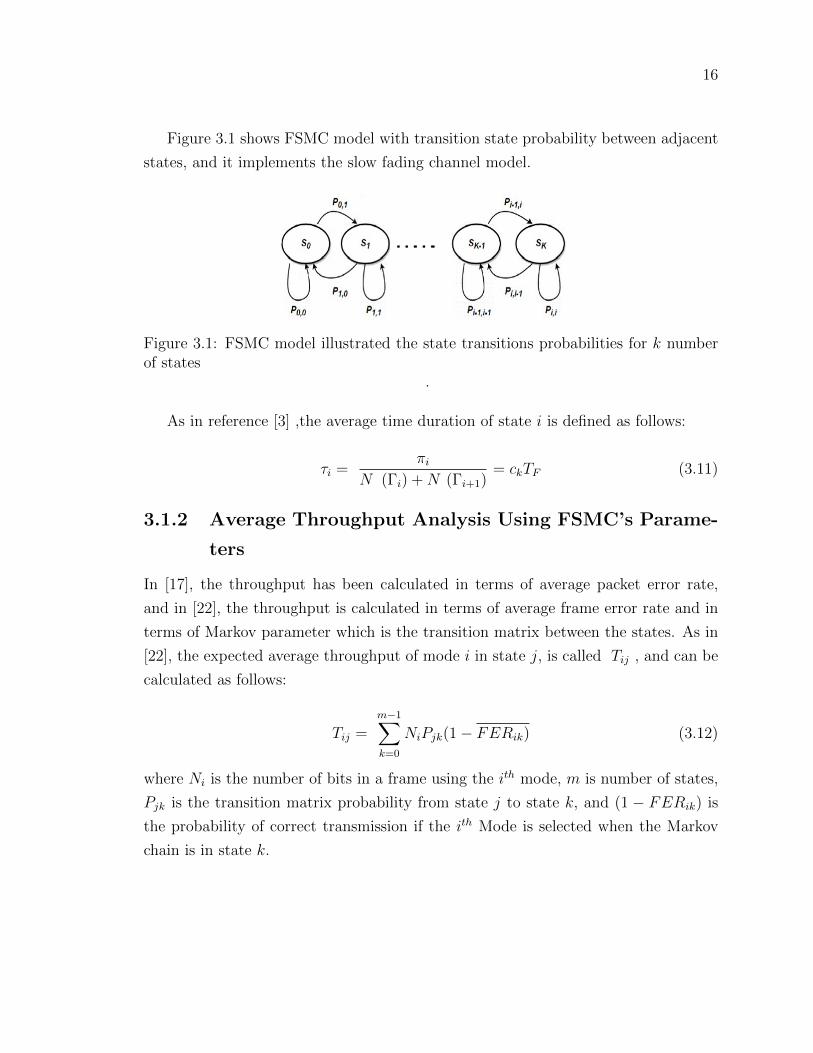
Figure 3.1 shows FSMC model with transition state probability between adjacent

states, and it implements the slow fading channel model.

Figure 3.1: FSMC model illustrated the state transitions probabilities for k numberof states

.

As in reference [3] ,the average time duration of state i is defined as follows:

τi =πi

N (Γi) +N (Γi+1)= ckTF (3.11)

3.1.2 Average Throughput Analysis Using FSMC’s Parame-

ters

In [17], the throughput has been calculated in terms of average packet error rate,

and in [22], the throughput is calculated in terms of average frame error rate and in

terms of Markov parameter which is the transition matrix between the states. As in

[22], the expected average throughput of mode i in state j, is called Tij , and can be

calculated as follows:

Tij =m−1∑k=0

NiPjk(1− FERik) (3.12)

where Ni is the number of bits in a frame using the ith mode, m is number of states,

Pjk is the transition matrix probability from state j to state k, and (1 − FERik) is

the probability of correct transmission if the ith Mode is selected when the Markov

chain is in state k.

17

Chapter 4

Channel Partitioning Methods of

FSMC

4.1 Signal to noise ratio partitioning

In this section, two different methods about SNR partition are presented. The first

one is called Steady State Equilibrium method,which is presented in [24][23], and the

second method is called Error Rate Curve Partitioning method. In this method, the

SNR is desecrated into levels (thresholds) regards to the curve of frame error rate

(FER) verses signal to noise ratio (SNR). The time interval of the frames is taken

into account.

4.1.1 Steady State Equilibrium Method

This method is also called Equal–Probability method and it is used to calculate the

channel thresholds of FSMC model. In this method, the SNR thresholds of the

channel are determined by [π1 = π2 = π3, . . . πi = 1/K]. Where, πi can be writing as

follows [24]:

πi = exp

(−Γiγ

)− exp

(−Γi+1

γ

)= 1/K. (4.1)

In the first case study of this project, we use this method to estimate the thresholds

(SNR) of the states to build the Markov model [24].

18

4.1.2 Error Rate Curve Partitioning Method

From the fact that the relationship between SNR and FER is a non linear curve as

shown in Figure 4.1, which shows the FER verses SNR curves for adaptive transmis-

sion system, uses three different M-QAM modulation schemes.

Figure 4.1: The FER verses SNR curves for adaptive transmission system, uses threedifferent M-QAM modulation schemes.

If we consider that an adaptive transmission wireless system works perfectly at

a certain FER, which is called target FER, we can calculate target SNR for each

curve by using equation (2.10). From Figure 4.1, we can determine three different

target SNR’s for each curve. These SNR’s can be considered as thresholds that the

adaptive transmission system uses to switch from current mode to other. The channel

performance of adaptive transmission systems can be evaluated using the Finite State

Markov Chain (FSMC) model. The target SNRs can be utilized as thresholds which

are used to calculate the parameter of FSMC model. Each mode can be considered as

a state in the FSMC model. In order to calculate the threshold of each state of FSMC

model, signal to noise ratio should be large enough for each state to cover the SNR

variation during a time frame T F . However, the signal to noise ratio ranges cannot be

too large so the states have different range of Frame error rates [24]. Based on these

19

considerations, there is a parameter used to calculate the time duration for a state in

order to estimate SNR partitioning. This parameter is called average time duration

τi, which is the average time interval of the received instantaneous SNR between two

thresholds (Γi − Γi+1). Average time duration τi is shown as follows [24]:

τi =πi

N (Γi) +N (Γi+1)= ckTF (4.2)

where ck is a constant and it is must be greater than 1. The constant ck can be

calculated by:

ck =1

TF

πiN (Γi) +N (Γi+1)

(4.3)

The SNR thresholds can be calculated using equations (2.12),(2.18), and it is called

main thresholds (adaptive modulation thresholds). The constants ck are calculated

from main thresholds, with regard to target FER and consultation size M . The

constant ck is large when the number of states is small and vice versa [5]. Form Figure

4.1, we have three main thresholds or four states which are not enough states to get

appropriate values of τi ; that’s because the range between (Γi − Γi+1) is large and

not uniform, which makes the parameter ck large too. We proved this phenomenon

in Figure 4.3, and it will be discussed later in the relationship between ck and SNR

thresholds section. For these reasons, we calculate new thresholds in order to get

reasonable values of ck and τi. These new thresholds are calculated for each mode or

state between (Γi − Γi+1) to consider the average time duration τi in the calculation.

These new thresholds introduce sub states in each mode or in each main state, and

they are chosen in order to ensure that the time duration of each sub state is not too

large or too small compared with the frame time duration T F . Now each mode has

sub states. The overall sub states for all modes are the new states for the system and

they will be used to calculate the parameters of the FSMC model for the adaptive

transition channel. The new thresholds can be calculated as in the following steps:

Step 1: calculate the main thresholds using formula (2.18).

Step 2: calculate the constant ck for each state from formula (4.3); if ck < 1 , end

the calculation , else if ck >1, go to step 3.

Step 3: calculate the sub thresholds for each mode as follows:

• Choose number of sub thresholds N of each mode.

• Set the vector {kn} = {1, 2, 3, . . . N}, where {kn} is number of sub thresholds

vector.

20

• Calculate the parameter Delta (∆n) for each mode as follows:

∆n = ((Γi+1 − Γi)/N), where i = [ 1, 2, 3, 4 , . . . N ] (4.4)

• Calculate the sub thresholds for each mode as follows:

γj = (Γi+(∆n×(kn (n)−1))), where n = [ 1, 2, . . . N ] , j = [1, 2, . . . K] (4.5)

where γj is the new sub thresholds of the FSMC channel model, ∆n is the step size

among sub thresholds (γj − γj+1). The main thresholds (Γi+1 − Γi) are assumed to

equal to adaptive transmission thresholds as we assumed previously in this method.

The parameters of the FSMC model can be calculated using the new thresholds (all

sub thresholds of all modes in one vector) where taking into account the time duration

of each state.

With this method we could eliminate the value of constant ck, and thus control

the average time duration τi , so it is reasonable value to calculate the thresholds of

the FSMC channel regards to the target FER of the system.

The advantages of this method are the flexibility of choosing the thresholds of the

channel directly from the target FER of the system , with low number of states K and

less average time duration τi. It can give a good evaluation for higher consultation

size of modulation schemes without increasing the number of states as in equilibrium

steady states method that we discussed previously. Average time duration τi can be

controllable using this method by changing the parameter (∆n). We can add value

of the parameter ∆n to SNR thresholds of adaptive modulation system to ensure the

best time to switch from one mode to another safely with respect the average time

duration among modes.

4.1.3 Relationship between Average Time Duration of a State

and SNR Thresholds of the Same State

Figure 4.2 and Figure 4.3 show the relationship between ck and the step size from

one state to another in FSMC model, which implement (Γi−Γi+1) range for different

values of SNR thresholds. In Figure 4.2, the step size for all states are small and

21

equal. Figure 4.3 shows the relation between ck and the step size of each state, with

non-uniform step size.

To plot these figures, we used equation (4.3) for different values of the thresholds

range (Γi − Γi+1). We set the number of thresholds K equal to nine, which gives

eight values of constant ck, and we plot the results in two cases. In the first case, we

assume the step size is equal for all states and is equal to delta (∆n). In the second

case we assume a random or non-equally step size. The values of Γi , ∆n and ck are

shown in Table 4.1, for the first case, and in Table 4.2 for the second case.

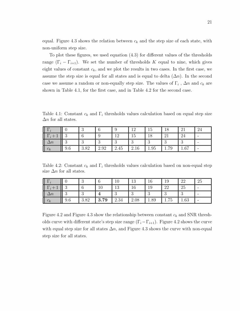
Table 4.1: Constant ck and Γi thresholds values calculation based on equal step size∆n for all states.

Γi 0 3 6 9 12 15 18 21 24

Γi+1 3 6 9 12 15 18 21 24 -

∆n 3 3 3 3 3 3 3 3 -

ck 9.6 3.82 2.92 2.45 2.16 1.95 1.79 1.67 -

Table 4.2: Constant ck and Γi thresholds values calculation based on non-equal stepsize ∆n for all states.

Γi 0 3 6 10 13 16 19 22 25

Γi+1 3 6 10 13 16 19 22 25 -

∆n 3 3 4 3 3 3 3 3 -

ck 9.6 3.82 3.79 2.34 2.08 1.89 1.75 1.63 -

Figure 4.2 and Figure 4.3 show the relationship between constant ck and SNR thresh-

olds curve with different state’s step size range (Γi−Γi+1). Figure 4.2 shows the curve

with equal step size for all states ∆n, and Figure 4.3 shows the curve with non-equal

step size for all states.

22

0 2 4 6 8 101

2

3

4

5

6

7

8

Sta

te i

nd

ex

C(k)

Figure 4.2: The relationship between constant ck and thresholds Γi with equal stepsize (∆n) for all states.

0 2 4 6 8 101

2

3

4

5

6

7

8

Sta

te i

nd

ex

C(k)

Figure 4.3: The relationship between constant ck and thresholds Γi with non-equalstep size (∆n) for all states.

23

Chapter 5

System Setup and Results

Discussion

5.1 Model of End to End Adaptive Modulation

System

Figure 5.1 shows end to end system connection from sender to receiver with a wire-

less link working with a single-transmit antenna and a single-receive antenna. Even

though we focus on Downlink systems here, the results are valid to Uplink systems

as well. A buffer with a first-in-first-out (FIFO) basis is used at the transmitter. The

buffer feeds the adaptive modulation (AM) controller, and the AM selector is fixed

at the receiver. We assume that the transmission has multiple modes to transmit

the data. Each mode represents a modulation format, and a forward error correction

code as in IEEE 802.11a. The AM selector determines the modulation mode based

on the channel state information (CSI) that is available at the destination, and sends

the decision back through a feedback channel to the AM controller to reselect the

transmission mode. A maximum likelihood decoding, and coherent demodulation are

used at the receiver. The decoded bits are mapped to packets so it can be pushed up

to layers above the physical layer.

24

Figure 5.1: End to End wireless link system model.

5.1.1 System Model Assumptions

1. The channel is frequency flat-slow fading. It keeps invariant per frame, but it

varies from one frame to another. The frame is a group of packets that contains the

bits stream. This assumption can be implemented by a block fading model that is

suitable for slow variation channel behavior. the AM mode is adjusted to change from

mode to another based on frame-by-frame basis.

2. We assume a perfect channel state (CSI) at the receiver, and the mode selection

is fed back to the AM controller without any latency or errors.

3. We assume the packets transmitted through a first in-first out queue. If the queue

become full, the new incoming packets will be dropped and will not be recovered or

retransmitted by end-to-end (sender to receiver) link. This assumption can be made

available by using User Datagram Protocol (UDP).

4. We assume perfect Cyclic Redundancy Check (CRC) will detect the error. The

CRC parity bits per packet is not incorporated in the throughput calculation.

5. The packet is dropped if it is not received correctly after error detection.

The aim of this project lies in finite-state-Markov modeling of received SNRs that

are assumed to follow Rayleigh fading distribution. Performance evaluation done by

finite state modeling and performance measures such as state time duration, state

transition probability, steady state probability, and level crossing rates are plotted

and presented.

25

5.2 Results of Steady State Equilibrium Partition-

ing Method

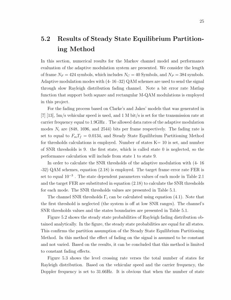
In this section, numerical results for the Markov channel model and performance

evaluation of the adaptive modulation system are presented. We consider the length

of frame NF = 424 symbols, which includes NC = 40 Symbols, and NP = 384 symbols.

Adaptive modulation modes with (4- 16 -32) QAM schemes are used to send the signal

through slow Rayleigh distribution fading channel. Note a bit error rate Matlap

function that support both square and rectangular M-QAM modulations is employed

in this project.

For the fading process based on Clarke’s and Jakes’ models that was generated in

[7] [13], 5m/s vehicular speed is used, and 1 M bit/s is set for the transmission rate at

carrier frequency equal to 1.9GHz . The allowed data rates of the adaptive modulation

modes Ni are (848, 1696, and 2544) bits per frame respectively. The fading rate is

set to equal to FmTf = 0.0134, and Steady State Equilibrium Partitioning Method

for thresholds calculations is employed. Number of states K= 10 is set, and number

of SNR thresholds is 9. the first state, which is called state 0 is neglected, so the

performance calculation will include from state 1 to state 9.

In order to calculate the SNR thresholds of the adaptive modulation with (4- 16

-32) QAM schemes, equation (2.18) is employed. The target frame error rate FER is

set to equal 10−3 . The state dependent parameters values of each mode in Table 2.1

and the target FER are substituted in equation (2.18) to calculate the SNR thresholds

for each mode. The SNR thresholds values are presented in Table 5.1.

The channel SNR thresholds Γi can be calculated using equation (4.1). Note that

the first threshold is neglected (the system is off at low SNR ranges). The channel’s

SNR thresholds values and the states boundaries are presented in Table 5.1.

Figure 5.2 shows the steady state probabilities of Rayleigh fading distribution ob-

tained analytically. In the figure, the steady state probabilities are equal for all states.

This confirms the partition assumption of the Steady State Equilibrium Partitioning

Method. In this method the effect of fading on the signal is assumed to be constant

and not varied. Based on the results, it can be concluded that this method is limited

to constant fading effects.

Figure 5.3 shows the level crossing rate verses the total number of states for

Rayleigh distribution. Based on the vehicular speed and the carrier frequency, the

Doppler frequency is set to 31.66Hz. It is obvious that when the number of state

26

1 2 3 4 5 6 7 8 9

0.2

0.4

0.6

0.8

1

State index

Ste

ad

y S

tate

Pro

ba

bili

tie

s

Figure 5.2: Steady state probabilities verses state index for Rayleigh fading channelusing steady state equilibrium partitioning method.

index increases, the SNRs increases, and the effects of the fading will be lower. From

the figure, the crossing rate increases from state 1 to state 3, and decreases from state

4 to 7. If the fading effect is low the channel will be considered good quality. The

crossing rate here depends on the value of the average SNR value and the thresholds

values, so the curve in the figure increases and decreases from the first state to the

last state regularly. this result is regenerated and is matched the results in [24].

Figure 5.4a, Figure 5.4b , and Figure 5.4c show the transition probabilities pi,i+1

, pi,i−1, and pi,i verses the states index. For the transition pi,i+1 the figure shows

the transitions from state 1 to 3 is increased and form state 4 to 7 decreased. For

the transition pi,i−1 , the figure shows the transitions from state 2 to 4 is increased

and form state 5 to 8 decreased. Note here the pi,i+1 = pi,i−1 ; this is because the

steady state probabilities for each state are equal. The probability of not making

any transition pi,i record high values, which represents slow fading, and it increases

when the number of states increases. these result are regenerated and are matched

the results in [24].

In Figure 5.5, the average frame error rates per states are presented. From Table

2.1, that includes the values of the state dependent parameters, aM , gM , and γpn for

all M-QAM modes, and from equations (2.17) , (2.19) and (3.7), We calculate the

actual average FER per state. Since the state index increases, the SNR increases and

27

1 2 3 4 5 6 7 8 95

10

15

20

25

30

35

State index

Nu

mb

ers

of

Cro

ssin

g R

ate

Figure 5.3: Number of crossing rate verses state index for Rayleigh fading channelusing steady state equilibrium partitioning method.

the average FER decreases. For the first mode which uses 4-QAM modulation scheme,

The channel introduces poor quality in the first two states, which is considered a noisy

channel that has significant effect on the received signal. States 3 to 9 introduce a

superior quality, which reflects the decreasing FER for these states. For the second

mode, which uses 16-QAM modulation scheme, the channel introduces poor quality

in the first four states, which is considered a noisy channel that has high effect on the

received signal. States 5 to 9 introduce improved quality. For the third mode, which

uses 32-QAM modulation scheme, the channel introduces poor quality from state 1

to state 7 , which is considered as noisy channel that effects on the received signal.

States 8 to 9 introduce a good quality.

Figure 5.6 shows the average throughput per state of each M-QAM mode of the

system model individually. First, we run 4-QAM modulation scheme of the adaptive

modulation system over all channel states and we calculate the average throughput

per each state, then we repeat this step with the 16-QAM and 32-QAM modulation

schemes modes respectively over all channel states. For all modes, we can see the

average throughput at the first states are low, and they increase dramatically toward

last states. For each state, we can compare the average throughput of all modes;

so we can decide at which SNR range the system should switch among modes. In

Table 5.1, we record the best mode switches decisions to get the highest performance

28

1 2 3 4 5 6 7 80.06

0.08

0.1

0.12

0.14

0.16

State index

Pi,i+

1

(a) Transitions probabili-ties pi,i+1 verses state in-dex.

2 3 4 5 6 7 8 90.06

0.08

0.1

0.12

0.14

0.16

State index

Pi,i−

1

(b) Transitions probabili-ties pi,i−1 verses state in-dex.

1 2 3 4 5 6 7 8 90.7

0.75

0.8

0.85

0.9

0.95

State index

Pi,i

(c) Transitions probabili-ties pi,i verses state index.

Figure 5.4: The transition probabilities for Rayleigh fading channel using steady stateequilibrium partitioning method.

of the system. As in the table, we can see the best switching choice from 4-QAM

to 16-QAM is at state 4. In other words, the system should switch whenever the

received SNR is located in the SNR channel’s thresholds range of state 4. The best

time to switch from mode 16-QAM to 32-QAM is at state 7 and then it keeps going

to with 32-QAM mode.

In Table 5.1, Interesting result came up when we sign in the boundaries of the

adaptive modulation thresholds into the boundaries of the channel thresholds, es-

pecially at the state 4. The thresholds boundaries of the adaptive modulation to

switch from the first mode to the second is different compared with channel thresh-

olds Boundaries, and that is because we set the target FER a little bit high (10−3).

So at that mode threshold value, the average throughput is less than the average

throughput of the first mode, thus no switching.

The constant ck in all states recorded high values, which range between 3 and 9.

The constant ck in this method is not controllable, so we cannot ensure the average

time duration of state k is a reasonable value.

29

1 2 3 4 5 6 7 8 910

−6

10−5

10−4

10−3

10−2

10−1

100

State index

Avera

ge F

ER

4QAM −mode1

16−QAM− mode2

32QAM−mode3

Figure 5.5: Average frame error rate per mode verses state index for the steady stateequilibrium partitioning method.

1 2 3 4 5 6 7 8 90

500

1000

1500

2000

2500

State index

Ave

rage T

hro

ughput in

bits

Throughput for mode 1



Figure 5.6: Average throughput per state in bits of each mode in case target FER =10−3 for the steady state equilibrium partitioning method.

30

Table 5.1: Values of channel thresholds and the adaptive modulation thresholds attarget FER = 10−3 calculated using steady state equilibrium partitioning method.

Channel thresholds(Γi)db

Selected mode Mode’s thresholds (γM)db Constant(ck)

6.4763 4-QAM 6.5349 < γt1 < 10.3021 4.5855

9.1941 4-QAM 6.5349 < γt1 < 10.3021 4.03415

11.0412 4-QAM 6.5349 < γt1 < 10.3021 3.8774

12.5107 16-QAM 10.3021 < γt2 < 13.5125 3.95230

13.7905 16-QAM 10.3021 < γt2 < 13.5125 4.2521

14.9854 16-QAM 10.3021 < γt2 < 13.5125 4.8801

16.1815 32-QAM 13.5125 < γt3 < INF 6.1901

17.4980 32-QAM 13.5125 < γt3 < INF 9.7727

19.2715 32-QAM 13.5125 < γt3 < INF -

5.3 Results of Error Rate Curve Partitioning

Method

In this section, numerical results of the system performance evaluation and the

Markov channel (FSMC) model are presented. We consider the same system model

and the same scenario as the previous method except the channel partitioning method

is changed to become Error Rate Curve Partitioning method. We assume mode 0 in

Figure 4.1 is neglected, so the SNR thresholds γm , which in this case study assumed

as Γi, start from mode 1 to mode 3. In addition, we assume there are two cases

based on target FER. The first case assumed the target FER= 10−3, and second case

assumed the target FER= 10−6. These two cases applied to all modes individually.

The effect of fading on the signal is assumed to be varied.

We first set the Target Frame error rate equal to 10−3. We calculated the parame-

ters of the FSMC channel model and the performance evaluation of the system based

on this setting, then we did the same procedure using Target FER = 10−6 to compare

the average throughput of the first case with the second case . Note that when we

change the value of the target FER , the thresholds of the channel will be changed,

so the parameters of the channel will also be changed. In this work, we only present

the channel parameter from the first case. The steady state probability, which is the

probability of being in state k, depending on the available number of FSMC states,

which is presented for the first case. Figure 5.7 shows the steady state probabilities

31

of 9 states available for FSMC. The probabilities of states 1, 2, and 3 are pretty close.

This means there is no switching among modulation modes in these states. States 4,

7, and 9 record the highest values among the states, which means at these states the

modulation mode should be switched.

1 2 3 4 5 6 7 8 9

0.2

0.4

0.6

0.8

1

State index

Ste

ad

y S

tate

Pro

ba

bili

tie

s

Figure 5.7: Steady state probabilities verses states in case target FER= 10−3 usingerror rate curve partitioning method.

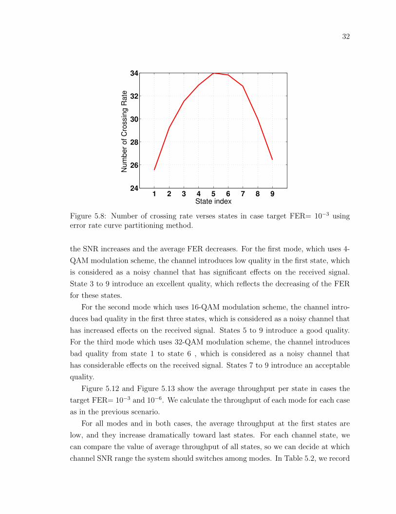
Figure 5.8 shows the level crossing rate verses the total number of states for

Rayleigh distribution. The Doppler frequency is set to equal 31.66Hz. From the

figure, the crossing rate increases from state 1 to state 3, and decreases from state 5

to 9. If the fading effect is low, the channel will be considered as good quality.

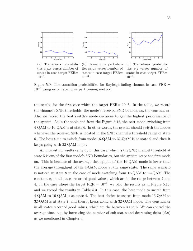
Figure 5.9a , Figure 5.9b, and Figure 5.9c show the transition probabilities pi,i+1

, pi,i−1, and pi,i verses the total number of states. Figure 5.9a, shows the transitions

of pi,i+1. The figure shows the transitions from state 1 to state 3 randomly increases,

and from states 4 to 7 randomly decreases compared with state 3. Figure 5.9b shows

the transitions of pi,i−1, the figure shows the transitions from states 2 to 3 increases,

and from states 4 to 9 randomly decreases compared with state 3. The probability of

not making any transition pi,i is shown in Figure 5.9c. It records high values which

represents slow fading, and it increases when the number of states increases.

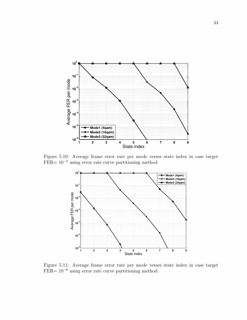
In Figure 5.10, the average frame error rate per states is presented. As in the

previous section, we calculate the actual average FER per state by substituting the

parameter in Table 2.1 in equations (2.17) and (3.7) . Since the state index increases,

32

1 2 3 4 5 6 7 8 924

26

28

30

32

34

State index

Nu

mb

er

of

Cro

ssin

g R

ate

Figure 5.8: Number of crossing rate verses states in case target FER= 10−3 usingerror rate curve partitioning method.

the SNR increases and the average FER decreases. For the first mode, which uses 4-

QAM modulation scheme, the channel introduces low quality in the first state, which

is considered as a noisy channel that has significant effects on the received signal.

State 3 to 9 introduce an excellent quality, which reflects the decreasing of the FER

for these states.

For the second mode which uses 16-QAM modulation scheme, the channel intro-

duces bad quality in the first three states, which is considered as a noisy channel that

has increased effects on the received signal. States 5 to 9 introduce a good quality.

For the third mode which uses 32-QAM modulation scheme, the channel introduces

bad quality from state 1 to state 6 , which is considered as a noisy channel that

has considerable effects on the received signal. States 7 to 9 introduce an acceptable

quality.

Figure 5.12 and Figure 5.13 show the average throughput per state in cases the

target FER= 10−3 and 10−6. We calculate the throughput of each mode for each case

as in the previous scenario.

For all modes and in both cases, the average throughput at the first states are

low, and they increase dramatically toward last states. For each channel state, we

can compare the value of average throughput of all states, so we can decide at which

channel SNR range the system should switches among modes. In Table 5.2, we record

33

1 2 3 4 5 6 7 8

0.2

0.4

0.6

0.8

1

State index

Pn,n

+1

(a) Transitions probabili-ties pi,i+1 verses number ofstates in case target FER=10−3.

2 3 4 5 6 7 8 9

0.2

0.4

0.6

0.8

1

State index

Pn,n

−1

(b) Transitions probabili-ties pi,i−1 verses number ofstates in case target FER=10−3.

1 2 3 4 5 6 7 8 9

0.2

0.4

0.6

0.8

1

State index

Pn,n

(c) Transitions probabili-ties pi,i verses number ofstates in case target FER=10−3.

Figure 5.9: The transition probabilities for Rayleigh fading channel in case FER =10−3 using error rate curve partitioning method.

the results for the first case which the target FER= 10−3. In the table, we record

the channel’s SNR thresholds, the mode’s received SNR boundaries, the constant ck.

Also we record the best switch’s mode decisions to get the highest performance of

the system. As in the table and from the Figure 5.12, the best mode switching from

4-QAM to 16-QAM is at state 6. In other words, the system should switch the modes

whenever the received SNR is located in the SNR channel’s threshold range of state

6. The best time to switch from mode 16-QAM to 32-QAM is at state 9 and then it

keeps going with 32-QAM mode.

An interesting results came up in this case, which is the SNR channel threshold at

state 5 is out of the first mode’s SNR boundaries, but the system keeps the first mode

on. This is because of the average throughput of the 16-QAM mode is lower than

the average throughput of the 4-QAM mode at the same state. The same scenario

is noticed in state 8 in the case of mode switching from 16-QAM to 32-QAM. The

constant ck in all states recorded good values, which are in the range between 2 and

4. In the case where the target FER = 10−6, we plot the results as in Figure 5.13,

and we record the results in Table 5.3. In this case, the best mode to switch from

4-QAM to 16-QAM is at state 4. The best choice to switch from mode 16-QAM to

32-QAM is at state 7, and then it keeps going with 32-QAM mode. The constant ck

in all states recorded good values, which are the between 3 and 5. We can control the

average time step by increasing the number of sub states and decreasing delta (∆n)

as we mentioned in Chapter 4.

34

1 2 3 4 5 6 7 8 910

−6

10−5

10−4

10−3

10−2

10−1

100

State index

Ave

rag

e F

ER

pe

r m

od

e

Mode1 (4qam)

Mode2 (16qam)

Mode3 (32qam)

Figure 5.10: Average frame error rate per mode verses state index in case targetFER= 10−3 using error rate curve partitioning method

1 2 3 4 5 6 7 8 910

−6

10−5

10−4

10−3

10−2

10−1

100

State index

Avera

ge F

ER

per

mode

Mode1 (4qam)

Mode2 (16qam)

Mode3 (32qam)

Figure 5.11: Average frame error rate per mode verses state index in case targetFER= 10−6 using error rate curve partitioning method

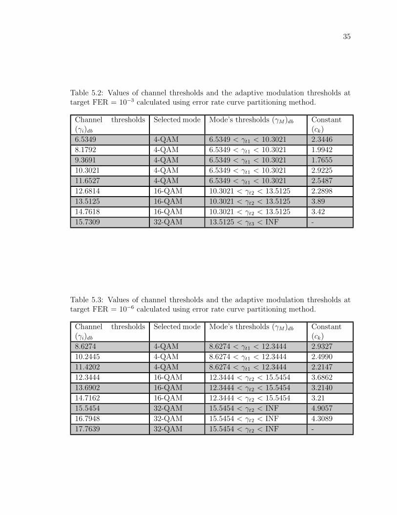
35

Table 5.2: Values of channel thresholds and the adaptive modulation thresholds attarget FER = 10−3 calculated using error rate curve partitioning method.

Channel thresholds(γi)db


6.5349 4-QAM 6.5349 < γt1 < 10.3021 2.3446

8.1792 4-QAM 6.5349 < γt1 < 10.3021 1.9942

9.3691 4-QAM 6.5349 < γt1 < 10.3021 1.7655

10.3021 4-QAM 6.5349 < γt1 < 10.3021 2.9225

11.6527 4-QAM 6.5349 < γt1 < 10.3021 2.5487

12.6814 16-QAM 10.3021 < γt2 < 13.5125 2.2898

13.5125 16-QAM 10.3021 < γt2 < 13.5125 3.89

14.7618 16-QAM 10.3021 < γt2 < 13.5125 3.42

15.7309 32-QAM 13.5125 < γt3 < INF -

Table 5.3: Values of channel thresholds and the adaptive modulation thresholds attarget FER = 10−6 calculated using error rate curve partitioning method.

Channel thresholds(γi)db


8.6274 4-QAM 8.6274 < γt1 < 12.3444 2.9327

10.2445 4-QAM 8.6274 < γt1 < 12.3444 2.4990

11.4202 4-QAM 8.6274 < γt1 < 12.3444 2.2147

12.3444 16-QAM 12.3444 < γt2 < 15.5454 3.6862

13.6902 16-QAM 12.3444 < γt2 < 15.5454 3.2140

14.7162 16-QAM 12.3444 < γt2 < 15.5454 3.21

15.5454 32-QAM 15.5454 < γt2 < INF 4.9057

16.7948 32-QAM 15.5454 < γt2 < INF 4.3089

17.7639 32-QAM 15.5454 < γt2 < INF -

36

1 2 3 4 5 6 7 8 90

500

1000

1500

2000

2500

State index

Ave

rag

e T

hro

ug

hp

ut

in b

its




Figure 5.12: Average Throughput per state in bits of each mode in case target FER=10−3 using error rate curve partitioning method

1 2 3 4 5 6 7 8 90

500

1000

1500

2000

2500

State index

Ave

rag

e T

hro

ug

hp

ut

in b

its




Figure 5.13: Average throughput per state in bits of each mode in case target FER=10−6 using error rate curve partitioning method.

37

Chapter 6

Conclusion

In this project, we presented adaptive modulation for end to end wireless link system,

which uses M-QAM modulation scheme over Rayleigh fading channel. We discussed

the mechanism of selecting the modulation schemes of adaptive modulation system ,

which maintain appropriate frame error rate, according to the channel state.

Finite State Markov Chain (FSMC) model is used to model the channel states in

terms of SNR. We presented two different FSMC channel petitioning methods. The

first method is called Equilibrium Steady State method. We discussed the FSMC

parameters of this method, and we used them to evaluate the system performance.

In this method, the fading effects on the received signal is assumed to be constant,

which means this method is specific to constant fading effects. Also, the average time

duration of the channel state is not included in the SNR thresholds calculation. The

second method is a new method for partitioning the SNRs of the channel states. It

is used in order to get best choice of modulation scheme selection for the adaptive

modulation system. In this method, we select the SNR levels of the channel based

on a desired FER of the system with respect to the average time of channel state

duration. We also introduce the relationship between the average time of channel

state duration and the SNR levels.

The advantages of this method are the flexibility of choosing the thresholds of the

channel directly from the desired (target) FER of the system, with lower number of

states (K) and less average time duration τi. It can give a good evaluation for higher

consultation size of modulation schemes without increasing the number of states K

as in Equilibrium Steady States method that we motioned previously. Average time

38

duration τi can be controllable using this method by changing the parameter Delta

(∆n).

For both methods, we discuss channel parameters and formulas that show the

behaviors of channels. Then we use these parameters to evaluate the performance of

the adaptive modulation system model. Performance measures of the FSMC model

such as state time duration, state transition probability, steady state probability, and

crossing rate for Rayleigh distribution are derived, plotted and analyzed. The average

FER for each channel state and the average throughput per channel state for each

modulation scheme (mode) are plotted. The numerical results of both methods are

compared and discussed.

39

Bibliography

[1] Mohamed-Slim Alouini and Andrea J Goldsmith. “Adaptive modulation over

Nakagami fading channels”. In: Wireless Personal Communications 13.1-2 (2000),

pp. 119–143.

[2] Vidhyacharan Bhaskar. “Finite-state Markov model for lognormal, chi-square

(central), chi-square (non-central), and K-distributions”. In: International Jour-

nal of Wireless Information Networks 14.4 (2007), pp. 237–250.

[3] Vidhyacharan Bhaskar and Nagireddy Peram. “Performance modeling of finite

state Markov chains for Nakagami-q and α–µ distributions over adaptive mod-

ulation and coding schemes”. In: AEU-International Journal of Electronics and

Communications 67.1 (2013), pp. 64–71.

[4] Kyongkuk Cho and Dongweon Yoon. “On the general BER expression of one-

and two-dimensional amplitude modulations”. In: IEEE Transactions on Com-

munications 50.7 (2002), pp. 1074–1080.

[5] Michael J Chu, Dennis L Goeckel, and Wayne E Stark. “On the design of Markov

models for fading channels”. In: Vehicular Technology Conference, 1999. VTC

1999-Fall. IEEE VTS 50th. Vol. 4. IEEE. 1999, pp. 2372–2376.

[6] Seong Taek Chung and Andrea J Goldsmith. “Degrees of freedom in adaptive

modulation: a unified view”. In: IEEE Transactions on Communications 49.9

(2001), pp. 1561–1571.

[7] RH Clarke. “A statistical theory of mobile-radio reception”. In: Bell Labs Tech-

nical Journal 47.6 (1968), pp. 957–1000.

[8] IEEE LAN/MAN Standards Committee et al. “IEEE Standard for local and

metropolitan area networks Part 16: Air interface for fixed and mobile broad-

band wireless access systems amendment 2: Physical and medium access control

BIBLIOGRAPHY 40

layers for combined fixed and mobile operation in licensed bands and corrigen-

dum 1”. In: IEEE Std 802.16-2004/Cor 1-2005 (2006).

[9] Angela Doufexi et al. “A comparison of the HIPERLAN/2 and IEEE 802.11

a wireless LAN standards”. In: IEEE Communications magazine 40.5 (2002),

pp. 172–180.

[10] Jason D Ellis, Michael A Juang, and Michael B Pursley. “Analytical evaluation

of adaptive coding for Markov models of Nakagami fading”. In: Information

Theory and Applications Workshop (ITA), 2012. IEEE. 2012, pp. 147–151.

[11] Andrea J Goldsmith and Soon-Ghee Chua. “Variable-Rate Variable-Power

M-QAM for fading channels”. In: IEEE transactions on communications 45.10

(1997), pp. 1218–1230.

[12] Kjell Jorgen Hole, Henrik Holm, and Geir E Oien. “Adaptive multidimensional

coded modulation over flat fading channels”. In: IEEE Journal on Selected Areas

in Communications 18.7 (2000), pp. 1153–1158.

[13] William C Jakes and Donald C Cox. Microwave mobile communications. Wiley-

IEEE Press, 1994.

[14] Michael A Juang and Michael B Pursley. “New results on finite-state Markov

models for Nakagami fading channels”. In: Military Communication Conference,

2011-MILCOM 2011. IEEE. 2011, pp. 453–458.

[15] Jeyhan Karaoguz. “High-rate wireless personal area networks”. In: IEEE com-

munications Magazine 39.12 (2001), pp. 96–102.

[16] Farooq Khan. LTEfor 4G mobile broadband: air interface technologies and per-

formance. Cambridge University Press, 2009.

[17] Qingwen Liu, Shengli Zhou, and Georgios B Giannakis. “Queuing with adaptive

modulation and coding over wireless links: cross-layer analysis and design”. In:

IEEE transactions on wireless communications 4.3 (2005), pp. 1142–1153.

[18] Michael B Pursley and John M Shea. “Adaptive nonuniform phase-shift-key

modulation for multimedia traffic in wireless networks”. In: IEEE Journal on

Selected Areas in Communications 18.8 (2000), pp. 1394–1407.

[19] Parastoo Sadeghi et al. “Finite-state Markov modeling of fading channels-a

survey of principles and applications”. In: IEEE Signal Processing Magazine

25.5 (2008).

BIBLIOGRAPHY 41

[20] Hong Shen Wang and Nader Moayeri. “Finite-state Markov channel-a useful

model for radio communication channels”. In: IEEE transactions on vehicular

technology 44.1 (1995), pp. 163–171.

[21] Hong-Chuan Yang and Mohamed-Slim Alouini. Order statistics in wireless com-

munications: diversity, adaptation, and scheduling in MIMO and OFDM sys-

tems. Cambridge University Press, 2011.

[22] James Yang, Amir K Khandani, and Noel Tin. “Statistical decision making in

adaptive modulation and coding for 3G wireless systems”. In: IEEE Transac-

tions on Vehicular Technology 54.6 (2005), pp. 2066–2073.

[23] Jungnam Yun and Mohsen Kavehrad. “Markov error structure for throughput

analysis of adaptive modulation systems combined with ARQ over correlated

fading channels”. In: IEEE Transactions on Vehicular Technology 54.1 (2005),

pp. 235–245.

[24] Qinqing Zhang and Saleem A Kassam. “Finite-state Markov model for Rayleigh

fading channels”. In: IEEE Transactions on communications 47.11 (1999), 1688

–1692.

Performance Evaluation for Adaptive Modulation Wireless ...

Documents