PERFORMANCE EVALUATION AND MODELING OF TWIN SCREW PUMPS A Dissertation by PENG LIU Submitted to the Office of Graduate and Professional Studies of Texas A&M University in partial fulfillment of the requirements for the degree of DOCTOR OF PHILOSOPHY Chair of Committee, Gerald L. Morrison Committee Members, Andrea Strzelec Je-Chin Han Robert Randall Head of Department, Andreas A. Polycarpou May 2016 Major Subject: Mechanical Engineering Copyright 2016 Peng Liu

Welcome message from author
This document is posted to help you gain knowledge. Please leave a comment to let me know what you think about it! Share it to your friends and learn new things together.
Transcript

PERFORMANCE EVALUATION AND MODELING OF TWIN SCREW PUMPS
A Dissertation
by
PENG LIU
Submitted to the Office of Graduate and Professional Studies of
Texas A&M University
in partial fulfillment of the requirements for the degree of
DOCTOR OF PHILOSOPHY
Chair of Committee, Gerald L. Morrison
Committee Members, Andrea Strzelec
Je-Chin Han
Robert Randall
Head of Department, Andreas A. Polycarpou
May 2016
Major Subject: Mechanical Engineering
Copyright 2016 Peng Liu
ii
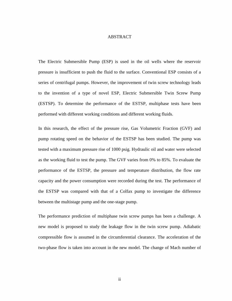
ABSTRACT
The Electric Submersible Pump (ESP) is used in the oil wells where the reservoir
pressure is insufficient to push the fluid to the surface. Conventional ESP consists of a
series of centrifugal pumps. However, the improvement of twin screw technology leads
to the invention of a type of novel ESP, Electric Submersible Twin Screw Pump
(ESTSP). To determine the performance of the ESTSP, multiphase tests have been
performed with different working conditions and different working fluids.
In this research, the effect of the pressure rise, Gas Volumetric Fraction (GVF) and
pump rotating speed on the behavior of the ESTSP has been studied. The pump was
tested with a maximum pressure rise of 1000 psig. Hydraulic oil and water were selected
as the working fluid to test the pump. The GVF varies from 0% to 85%. To evaluate the
performance of the ESTSP, the pressure and temperature distribution, the flow rate
capacity and the power consumption were recorded during the test. The performance of
the ESTSP was compared with that of a Colfax pump to investigate the difference
between the multistage pump and the one-stage pump.
The performance prediction of multiphase twin screw pumps has been a challenge. A
new model is proposed to study the leakage flow in the twin screw pump. Adiabatic
compressible flow is assumed in the circumferential clearance. The acceleration of the
two-phase flow is taken into account in the new model. The change of Mach number of
iii
the leakage flow in the clearance and the possibility of choked flow at the outlet of the
clearance will be studied.
To verify the leakage model, experimental data of four different twin screw pumps is
used to compare with the prediction by the model.

iv
DEDICATION
To my dear wife — for her support of all that I do
v
ACKNOWLEDGEMENTS
My study at Texas A&M University will soon come to an end. At the completion of my
dissertation, I wish to express my sincere gratitude to all those who have offered my
invaluable assistance during the three years in the Turbomachinery Lab.
First, I would like to express my gratitude to Dr. Gerald Morrison, my supervisor, for his
guidance and encouragement. He always supported me with intelligence and expertise
whenever I met with difficulties.
Also, I would like to thank my committee members, Dr. Andrea Strzelec, Dr. Je-Chin
Han and Dr. Robert E. Randall, for their guidance and support throughout this research.
Thanks to Dr. Jun Xu at Shell Exploration & Production and Dr. Pradeep Dass at Can-K
Group of companies for their continuous inputs and supports of this project. Thanks also
to my friends Klayton Kirkland, Scott Chien, Sahand Prouzpaneh, Sujan Reddy, Yi
Chen, and Wenfei Zhang for making my time at Texas A&M University a great
experience.
Finally, thanks to my mother and father for their encouragement and to my wife for her
patience and love.

vi
NOMENCLATURE
ASD Adjustable speed drive
CFD Computational fluid dynamics
CC Circumferential clearance
FC Flank clearance
RC Root clearance or radial clearance
ESP Electric submersible pump
ESTSP Electric submersible twin screw pump
GVF Gas volume fraction
GUI Graphical user interface
Re Reynolds number
P&ID Pipe and instruments diagram
M Mach number
N Total stage
K Roughness factor
T Temperature
𝑄 Flow rate
V Volume
𝑃𝑑𝑟𝑖𝑣𝑒 Drive power
𝑃𝑛𝑒𝑡, 𝑖𝑠𝑜𝑡ℎ𝑒𝑟𝑚𝑎𝑙 Work done for isothermal compression
𝑃𝑛𝑒𝑡, 𝑝𝑜𝑙𝑦𝑡𝑟𝑜𝑝𝑖𝑐 Work done for polytropic compression
vii
𝑄𝑠,𝑖 Leakage across screw i
𝐴𝑠,𝑡 Effective leakage area in the circumferential clearance
𝑋𝑃 Mass fraction
𝑋 Friction factor
𝑍 Compressibility factor
𝑈 Internal energy
𝜙𝐿2 Two-phase friction multiplier
∆𝑡 Time step
𝑐 Speed of sound
𝑐𝑝 Specific heat of constant pressure
𝑐𝑣 Specific heat of constant volume
𝑑ℎ Hydraulic diameter
𝑓 Friction factor
ℎ Enthalpy
𝑙 Clearance length
∆𝑝 Differential pressure
𝑝 Pressure
𝑣 Velocity
�� Mass flow rate
𝑛 Polytropic coefficient
𝑠 Width of the clearance
𝑣 Velocity

viii
𝑘𝑒 Loss coefficient
𝑓𝑡 Ratio of circumferential leakage to total leakage
y Gap depth
𝑚ℎ Half of hydraulic mean gap
𝑛𝑝 Screw number
𝜔 Pump speed
𝛼 GVF
𝜂𝑣 Volumetric efficiency
𝜂𝑚𝑒𝑐ℎ Mechanical efficiency
𝜂𝑒𝑓𝑓 Pump effectiveness
𝜌 Density
𝜇𝑚 Viscosity
𝜏 Period of one revolution
Subscript
𝑙 Liquid
𝑔 Gas
𝑖𝑛 Inlet
𝑜𝑢𝑡 Outlet
𝑖 Chamber index
0 Chamber condition
𝑚 Mean value
𝑡 Time

ix
𝑁 Iteration number
𝑤 Water
𝑜 Oil
𝑟𝑒𝑣 Revolution
𝑡ℎ Theoretical
𝑎 Actual
𝑟 Recirculation
x
TABLE OF CONTENTS
Page
ABSTRACT .......................................................................................................................ii
DEDICATION .................................................................................................................. iv
ACKNOWLEDGEMENTS ............................................................................................... v
NOMENCLATURE .......................................................................................................... vi
TABLE OF CONTENTS ................................................................................................... x
LIST OF FIGURES ..........................................................................................................xii
LIST OF TABLES .........................................................................................................xvii
1 INTRODUCTION ...................................................................................................... 1
1.1 Introduction of Twin Screw Pumps ..................................................................... 4
1.2 Literature Review ................................................................................................ 6
1.2.1 Experiment and Modeling ............................................................................ 6
1.2.2 Two Phase Flow ......................................................................................... 21
2 OBJECTIVES .......................................................................................................... 22
3 FUNDAMENTALS OF TWIN SCREW PUMP ..................................................... 24
3.1 The Geometry Parameters of the Screws .......................................................... 25
3.2 Volumetric Efficiency ....................................................................................... 27
3.3 Mechanical Efficiency ....................................................................................... 29
3.4 Pump Effectiveness ........................................................................................... 30
4 METHODOLOGY ................................................................................................... 32
4.1 Experimental Set Up .......................................................................................... 32
4.1.1 Test Rigs ..................................................................................................... 32
4.1.2 Instrumentations ......................................................................................... 38
4.1.3 Data Acquisition System ............................................................................ 42
4.2 Test Matrix ........................................................................................................ 44
5 PERFORMANCE EVALUATION OF EXPERIMENTAL RESULTS ................. 48

xi
5.1 Power Consumption .......................................................................................... 48
5.2 Pressure and Temperature Distribution ............................................................. 52
5.3 Volumetric Flow Rate Capacity ........................................................................ 58
5.4 Volumetric Efficiency ....................................................................................... 62
5.5 Mechanical Efficiency ....................................................................................... 66
5.6 Pump Effectiveness ........................................................................................... 72
5.7 Leakage Flow Rate ............................................................................................ 74
5.8 Comparison of the Water Tests ......................................................................... 77
5.9 Performance Comparison of Colfax Pump and Can-K Pump ........................... 81
5.9.1 Volumetric Flow Rate Capacity ................................................................. 81
5.9.2 Leakage Flow Rate ..................................................................................... 82
5.9.3 Volumetric Efficiency ................................................................................ 84
5.9.4 Mechanical Efficiency ................................................................................ 88
6 MULTIPHASE TWIN-SCREW PUMP MODEL ................................................... 90
6.1 Simplification of Twin Screw Pump Working Process ..................................... 91
6.2 Geometric Parameters ........................................................................................ 92
6.3 Leakage Flow in the Clearance ......................................................................... 94
6.4 Sonic Speed of Homogeneous Two Phase Flow ............................................... 99
6.5 Mass Balance in the Chambers ........................................................................ 100
6.6 Solution Methodology ..................................................................................... 102
6.7 Modeling of Multistage Twin Screw Pump .................................................... 104
7 MULTIPHASE TWIN-SCREW PUMP MODEL VALIDATION ....................... 105
7.1 Prediction of Pressure Distribution in the Twin Screw Pump ......................... 105
7.2 Volumetric Efficiency Prediction of Colfax Pump ......................................... 108
7.3 Volumetric Efficiency Prediction of Can-K Pump .......................................... 111
7.4 Volumetric Efficiency Prediction of Leistritz Pump ....................................... 113
7.5 Volumetric Efficiency Prediction of Flowserve Pump .................................... 114
7.6 Mach Number Analysis ................................................................................... 116
7.7 Effect of Suction Pressure on Volumetric Efficiency ..................................... 120
7.8 Effect of Water Cut on Pump Performance ..................................................... 123
8 CONCLUSION ...................................................................................................... 126
8.1 Experimental .................................................................................................... 126
8.2 Analytical Model ............................................................................................. 127
8.3 Recommendations ........................................................................................... 128
REFERENCES ............................................................................................................... 129
APPENDIX A UNCERTAINTY ANALYSIS .............................................................. 133

xii
LIST OF FIGURES
Page
Figure 1.1 Conventional ESP [3] ..................................................................................... 2
Figure 1.2 Drawing of the Can-K 425 ESTSP ................................................................. 3
Figure 1.3 Cutaway of a multiphase twin-screw pump [6] .............................................. 5
Figure 1.4 Pressure distributions in the screw pump [4] .................................................. 8
Figure 1.5 Sectional drawing of a twin screw pump [19] .............................................. 18
Figure 3.1 Geometric parameters of the twin screw pump [23] ..................................... 25
Figure 3.2 Fluid volume created by intermeshed screws [23] ....................................... 26
Figure 3.3 Clearance types of the twin screw pumps [21] ............................................. 28
Figure 4.1 Flow loop diagram of water test ................................................................... 33
Figure 4.2 Motor ............................................................................................................ 34
Figure 4.3 Flow loop diagram of oil test ........................................................................ 35
Figure 4.4 Can-K 425 ESTSP and discharge valve ....................................................... 36
Figure 4.5 Water tank, heat exchanger and separator .................................................... 37
Figure 4.6 Pump and motor assembly (Klayton, 2013) ................................................. 38
Figure 4.7 LabVIEW front panel ................................................................................... 42
Figure 4.8 LabVIEW front panel (continue) .................................................................. 43
Figure 5.1 Effect of different speeds on power consumption at 10% GVF, 100%
water test ....................................................................................................... 49
Figure 5.2 Effect of GVF on power consumption at 4000 RPM, 100% water cut test .. 50
Figure 5.3 Effect of GVF on power consumption at 4000 RPM, 100% water cut test .. 51

xiii
Figure 5.4 Effect of water cut on power consumption at 4000 RPM, 10% GVF .......... 52
Figure 5.5 Pressure distributions at 4000 RPM, 100% water cut, 10% GVF ................ 53
Figure 5.6 Effect of GVF on pressure distribution at 4000 RPM, 100% water cut,
400 psig differential pressure ........................................................................ 54
Figure 5.7 Temperature distributions at 4000 RPM, 100% water cut, 10% GVF ......... 55
Figure 5.8 Effect of water cut on total temperature rise at 4000 RPM, 10% GVF ........ 56
Figure 5.9 Polytropic coefficient of different water cuts, 4000 RPM ............................ 57
Figure 5.10 Effect of water cut on polytropic coefficient at 4000 RPM, 20% GVF ....... 58
Figure 5.11 Effect of pump speed on volumetric flow rate capacity at 10% GVF,
100% water cut test ....................................................................................... 60
Figure 5.12 Volumetric flow rate capacity at 4000 RPM, 100% water test .................... 61
Figure 5.13 Volumetric flow rate capacity at 4000 RPM, pure oil test ........................... 61
Figure 5.14 Effect of water cut on volumetric flow rate capacity .................................... 62
Figure 5.15 Volumetric efficiency at 4000 RPM, 100% water cut test ........................... 64
Figure 5.16 Volumetric efficiency at 4000 RPM, 0% water cut test ............................... 65
Figure 5.17 Effect of speed on volumetric efficiency at 10% GVF, 100% Water Test ... 65
Figure 5.18 Effect of water cut on volumetric efficiency at 4000 RPM, 10% GVF ........ 66
Figure 5.19 Mechanical efficiency (isothermal) for 100% water cut test at 4000 RPM .. 67
Figure 5.20 Mechanical efficiency (isothermal) for 0% water cut test at 4000 RPM ...... 67
Figure 5.21 Power imparted into liquid and gas at different GVF of 100% water
cut test ........................................................................................................... 68
Figure 5.22 Friction losses of 100% water cut test .......................................................... 69
Figure 5.23 Effect of pump speed on mechanical efficiency (Isothermal) at 10%
GVF, 100% water test ................................................................................... 71
Figure 5.24 Effect of water cut on mechanical efficiency at 4000 RPM, 10% GVF ....... 72

xiv
Figure 5.25 Polytropic effectiveness for 100% water test at 4000 RPM ......................... 73
Figure 5.26 Polytropic effectiveness for 0% water cut test at 4000 RPM ....................... 73
Figure 5.27 Effect of pump speed on leakage flow for 100% water cut test ................... 75
Figure 5.28 Effect of water cut on leakage flow at 4000 RPM, 10% GVF ..................... 76
Figure 5.29 Comparison of volumetric flow rate capacity for 100% water test, 3550
RPM .............................................................................................................. 78
Figure 5.30 Comparison of volumetric flow rate capacity for 100% water test, 4000
RPM .............................................................................................................. 79
Figure 5.31 Effect of temperature on volumetric flow capacity ...................................... 80
Figure 5.32 Effect of speed on leakage flow for different GVF at 100 psig inlet
pressure, Colfax pump .................................................................................. 83
Figure 5.33 Volumetric efficiency of Colfax pump at 100 psig inlet pressure,
1800 RPM ..................................................................................................... 85
Figure 5.34 Volumetric efficiency for Colfax pump at 100 psig inlet pressure,
1800 RPM ..................................................................................................... 85
Figure 5.35 Volumetric efficiency for Can-K pump at 100 psig inlet pressure,
4000 RPM ..................................................................................................... 86
Figure 5.36 Comparison of skid based GVF and pump based GVF ................................ 87
Figure 5.37 Comparison of mechanical efficiency .......................................................... 89
Figure 6.1 Simplification of the twin screw pump ......................................................... 91
Figure 6.2 Leakage flow in the circumferential clearance ............................................. 95
Figure 6.3 Fluids acceleration in the entrance of clearance ........................................... 95
Figure 6.4 Computer program algorithm ....................................................................... 96
Figure 6.5 Control volume of fanno flow in the duct ..................................................... 97
Figure 6.6 Sonic speed of two phase water/air flow at 100 psig .................................. 100
Figure 6.7 Mass balance in one closed chamber .......................................................... 101

xv
Figure 6.8 Computer program algorithm ..................................................................... 103
Figure 7.1 Non-dimensional pressure distribution of Colfax pump with 15 psig
suction pressure ........................................................................................... 106
Figure 7.2 Non-dimensional pressure distribution of Colfax pump with 100 psig
suction pressure ........................................................................................... 107
Figure 7.3 Comparison of prediction and experimental results of Colfax pump
with 15 psig suction pressure ...................................................................... 109
Figure 7.4 Comparison of prediction and experimental results of Colfax pump
with 100 psig suction pressure .................................................................... 110
Figure 7.5 Comparison of prediction and experimental results of Can-K pump for
water test at 4000 RPM ............................................................................... 111
Figure 7.6 Comparison of prediction and experimental results of Can-K pump for
oil Test at 4000 RPM .................................................................................. 112
Figure 7.7 Comparison of prediction and experimental results of Can-K pump for
water test at 3550 RPM ............................................................................... 112
Figure 7.8 Comparison of prediction and experimental results of Can-K pump for
oil test at 3550 RPM ................................................................................... 113
Figure 7.9 Comparison of prediction and experimental results of Leistritz pump....... 114
Figure 7.10 Comparison of prediction and experimental results of Flowserve pump ... 115
Figure 7.11 Mach number in the Leistritz pump with 100 psig differential pressure .... 117
Figure 7.12 Mach number in the Leistritz pump with 250 psig differential pressure .... 118
Figure 7.13 Mach number in the Colfax pump at 200 psig differential pressure,
15 psig suction pressure .............................................................................. 119
Figure 7.14 Mach number in the Colfax pump at 200 psig differential pressure,
100 psig suction pressure ............................................................................ 120
Figure 7.15 Comparison of volumetric efficiency for Colfax pump with different
suction pressure (experimental data) .......................................................... 121
Figure 7.16 Comparison of pressure distribution for Colfax pump with different
suction pressure ........................................................................................... 122
xvi
Figure 7.17 Comparison of water/air sonic speed at 100 psig and 15 psig .................... 122
Figure 7.18 Prediction comparison of volumetric efficiency of water test and oil
test at 3550 RPM ......................................................................................... 124
Figure 7.19 Prediction comparison of volumetric efficiency of water test and oil
test at 4000 RPM ......................................................................................... 124
Figure 7.20 Comparison of Mach number for Can-K pump of water test and oil test
at 4000 RPM, 1000 psig differential pressure, 50% GVF .......................... 125
Figure 7.21 Comparison of sonic speed of water/ air and oil/ nitrogen at 100 psig ...... 125

xvii
LIST OF TABLES
Page
Table 4.1 Pressure transducers used in experimental testing ........................................... 39
Table 4.2 Flow meters for water test ................................................................................ 40
Table 4.3 Flow meters for oil/water test .......................................................................... 40
Table 4.4 Micro Motion CMFS015M accuracy and repeatability (Gas) ......................... 41
Table 4.5 Micro Motion CMFS075M accuracy and repeatability (Liquid) ..................... 41
Table 4.6 Micro Motion CMF200M accuracy and repeatability (Liquid) ....................... 41
Table 4.7 Specifications of the NI Modules and iServer Microserver ............................. 44
Table 4.8 Test matrix of water test ................................................................................... 45
Table 4.9 Test matrix of oil test, low GVF ...................................................................... 46
Table 4.10 Test matrix of oil test, high GVF ................................................................... 46

1
1 INTRODUCTION
In the oil industry, artificial lift is an effective tool to sustain and increase the production
of an oil well where the reservoir pressure is insufficient to drive the oil to the surface.
According to a survey result from Schlumberger, only approximately 5% of the one
million oil wells around the world flow naturally. [1] As a consequence, most of the oil
production in the world intensely relies upon the artificial lift technology. Artificial lift
has become a well-developed industry. However, innovations in artificial lift technology
continue to be developed to meet the increasing challenges in the petroleum industry. In
this chapter, the introduction of the main artificial lift methods will be presented. An
innovation in artificial lift methods arose recently which will be presented and the
related previous research will be summarized.
The most common artificial lift methods include rod pumps, gas lift, hydraulic pumps,
electrical submersible pumps (ESP), etc. [2] The rod pump system transfers well fluids
by a reciprocating piston (plunger). The plunger connects to the surface pumping unit by
a rod. The rod pump is simple and familiar to most operators, so it is used widely. But it
is limited in the wells with high GVF flow. The rod pump system needs a large surface
footprint and high capital investment. Also depth limited and directional drilling can
limit its usage.
The principle of gas lift is to inject compressed gas into the well to reduce the mixture
density. Thus, the backpressure is reduced and the reservoir pressure is able to push the

2
fluids up to the surface. The gas lift is highly flexible, and it is highly tolerant with sand.
However, the gas lift is limited in the oil wells with high back pressure.
The hydraulic pumping system conveys power to the downhole by pressurized fluid,
which drives the subsurface pump to push fluid. The hydraulic pump is expensive and it
is usually employed where other artificial methods are not available.
Electrical submersible pump system usually consists of subsurface pump (electrical
submersible pump), electrical motor, protector for motor, and surface control equipment.
The electric submersible pump is composed of multi-stages pumping units installed in
series.
Figure 1.1 Conventional ESP [3]

3
The ESP system is one of the most common artificial lift methods due to its high
efficiency and flexibility. The electric submersible pump is typically used to pump high
flow rates in the deep oil wells. Compared with other artificial lift equipment, the
electric submersible pump has significant advantages in the offshore application,
because it needs the least space of surface construction. [2] A typical ESP pump is
shown in Figure 1.1.
Figure 1.2 Drawing of the Can-K 425 ESTSP
The ESP technology has undertaken significant improvements since its invention in the
1910s. Conventional ESPs are composed of a series of centrifugal pumps as shown in
Figure 1.1. However, a new type of ESP has emerged recently due to the development of
twin screw pump technology. The Can-K Group of Companies Inc. designed and

4
manufactured an electrical submersible twin screw pump (ESTSP) to challenge the
traditional ESPs. The pump consists of 10 stages of twin screw pump elements in series.
As shown in Figure 1.2, the diameter of the ESTSP is designed very small to fit into the
oil well casing. In the downhole application, it is often required to handle high pressure
conditions. With multiple stages, the new twin screw pump contains a great number of
seals which enable it to keep its performance at high pressure operation. [4]
1.1 Introduction of Twin Screw Pumps
The twin screw pump is a type of positive displacement pump. It has two intermeshed
screws, which form a series of closed chambers with the surrounding housing. When the
pump runs, the liquid is carried by the moving chambers axially from the pump inlet to
the outlet. As a displacement pump, the twin screw pump can handle very high GVF
flow. In addition, the twin screw pump shows better erosion resistance due to the
relatively low fluid velocity in the pump. The twin screw pump has been one of the most
popular multiphase pumps in the petroleum industry.
Typically, there are two types of arrangements for twin screw pumps, single-end and
double-end. The double-end arrangement is more popular and has been widely used due
to its simplicity and compactness. As shown in Figure 1.3, the double-end pump is
composed by two opposed pump elements with a common driving rotor. The working
fluid flow through entrance and is absorbed into the pump elements at the both sides.
The two pump elements produce equal and opposite axial thrust eliminating the need for

5
axial thrust bearings. The double-end pump is widely used as surface pump in the
petroleum industry for the low and medium pressure multiphase pumping. [5]
Figure 1.3 Cutaway of a multiphase twin-screw pump [6]
Compared with double-end arrangement, the single-end arrangement usually has longer
screws. Hence, there are more closed chambers and seals in this type of pump. The
working fluid enters the pump at one end and it is discharged at the other end. With
more seals, the single-end pump has significant advantages to handle high pressure and
GVF applications. Also, the unique design makes the single-end pump able to be

6
employed for subsurface applications. This design does require large capacity thrust
bearing as shown in Figure 1.2.
The twin screw pump has been widely used for multiphase pumping in the petroleum
industry. Extensive research has been done to investigate the working principle of twin
screw pumps for multiphase flow.
1.2 Literature Review
1.2.1 Experiment and Modeling
Performance test and leakage flow analysis of the twin screw pump have been the
research focus over the past decades. Since the twin screw pump is a positive
displacement pump, theoretically it conveys a fixed volume of fluid in one revolution.
However, if there is a pressure rise from the pump inlet to outlet, leakage flow will occur
from the pump discharge side to the pump suction side through the internal clearances.
Thus, the actually flow rate of a twin screw pump is always less than the theoretical flow
rate. The leakage flow rate is usually affected by the dimensions of the clearances, the
liquid viscosity, the differential pressures, GVF, etc.
The leakage flow can impose a serious impact on the performance of twin screw pumps.
As a result, numerous experimental tests have been conducted to study its performance.
These experiments were basically performed with water and air. Analytical models and
CFD simulations have been proposed to understand the working principle of the leakage
flow. In this section, the previous research on the twin screw pump will be summarized.

7
Vetter and Wincek [7] investigated the performance of two commercial twin screw
pumps and they developed the first computer model to predict the pump performance for
both single and two phase operation. In the computer model, the compression process
was assumed to be isothermal due to the high specific heat of the liquid compared with
the gas. It was also assumed that all clearances are filled with liquid only. In addition,
the liquid backflow is the only factor that leads to the gas compression. The internal
leakage flow velocity was calculated according to the differential pressure between the
two adjacent cavities with the equation below,
Δ𝑝 = 𝑓𝑙
𝑑ℎ
𝜌𝑙
2𝑣2 1.1
where 𝜆 is the friction factor depending on the flow mode. For the laminar flow,
𝑓 =96
𝑅𝑒 1.2
For the turbulent smooth clearance,
𝑓 =0.3322
𝑅𝑒0.25 1.3
For the turbulent rough clearance, the friction factor can be found by
1
√𝑓= 2 ∙ 𝑙𝑜𝑔 (
2𝑠
𝐾) + 0.97 1.4
The steady state operating conditions were obtained by iteration. Figure 1.4 shows the
predicted pressure distributions by the computer model for single phase and two phase
flow.

8
Figure 1.4 Pressure distributions in the screw pump [4]
Vetter evaluated the multiphase performance of two commercial screw pumps from
Leistritz Corporation and Bornemann Corporation. The power consumption, isothermal
efficiency, and volumetric flow rate capacity were investigated in this study.
Vetter verified the model prediction with the experimental data. The prediction results
shows good agreement with experimental results when the inlet GVF is below 50%.
However, the predictions deviate from the experimental data at 50% and 90% GVFs. In
this case, the assumption of the totally liquid-filled clearances is no longer true and the
gas injection in the clearance should be considered.
9
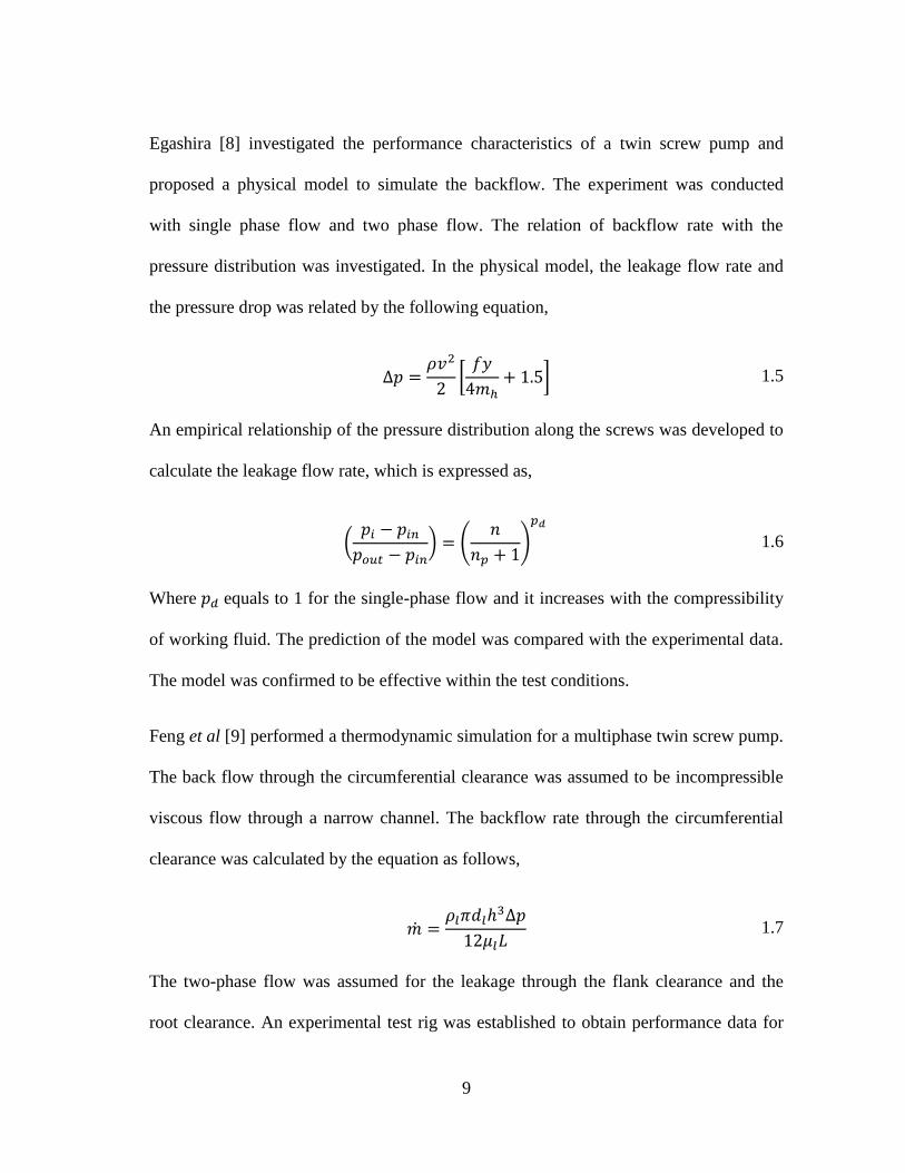
Egashira [8] investigated the performance characteristics of a twin screw pump and
proposed a physical model to simulate the backflow. The experiment was conducted
with single phase flow and two phase flow. The relation of backflow rate with the
pressure distribution was investigated. In the physical model, the leakage flow rate and
the pressure drop was related by the following equation,
∆𝑝 =𝜌𝑣2
2[
𝑓𝑦
4𝑚ℎ+ 1.5] 1.5
An empirical relationship of the pressure distribution along the screws was developed to
calculate the leakage flow rate, which is expressed as,
(𝑝𝑖 − 𝑝𝑖𝑛
𝑝𝑜𝑢𝑡 − 𝑝𝑖𝑛) = (
𝑛
𝑛𝑝 + 1)
𝑝𝑑
1.6
Where 𝑝𝑑 equals to 1 for the single-phase flow and it increases with the compressibility
of working fluid. The prediction of the model was compared with the experimental data.
The model was confirmed to be effective within the test conditions.
Feng et al [9] performed a thermodynamic simulation for a multiphase twin screw pump.
The back flow through the circumferential clearance was assumed to be incompressible
viscous flow through a narrow channel. The backflow rate through the circumferential
clearance was calculated by the equation as follows,
�� =𝜌𝑙𝜋𝑑𝑙ℎ
3Δ𝑝
12𝜇𝑙𝐿 1.7
The two-phase flow was assumed for the leakage through the flank clearance and the
root clearance. An experimental test rig was established to obtain performance data for
10
different operating conditions. Feng compared the simulation results and the
experimental data. The prediction showed good agreement with the test data within the
test conditions.
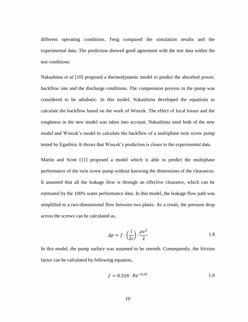
Nakashima et al [10] proposed a thermodynamic model to predict the absorbed power,
backflow rate and the discharge conditions. The compression process in the pump was
considered to be adiabatic. In this model, Nakashima developed the equations to
calculate the backflow based on the work of Wincek. The effect of local losses and the
roughness in the new model was taken into account. Nakashima used both of the new
model and Wincek’s model to calculate the backflow of a multiphase twin screw pump
tested by Egashira. It shows that Wincek’s prediction is closer to the experimental data.
Martin and Scott [11] proposed a model which is able to predict the multiphase
performance of the twin screw pump without knowing the dimensions of the clearances.
It assumed that all the leakage flow is through an effective clearance, which can be
estimated by the 100% water performance data. In this model, the leakage flow path was
simplified to a two-dimensional flow between two plates. As a result, the pressure drop
across the screws can be calculated as,
∆𝑝 = 𝑓 ∙ (𝑙
2𝑐) ∙
𝜌𝑣2
2 1.8
In this model, the pump surface was assumed to be smooth. Consequently, the friction
factor can be calculated by following equation,
𝑓 = 0.316 ∙ 𝑅𝑒−0.25 1.9
11
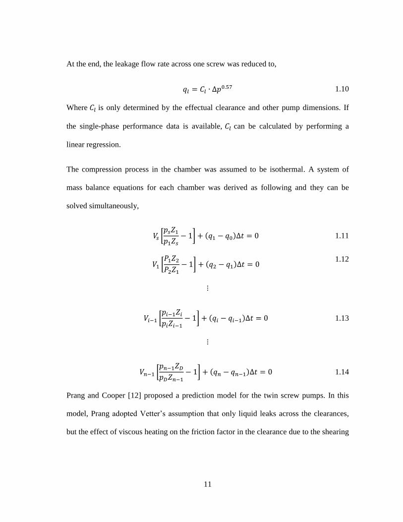
At the end, the leakage flow rate across one screw was reduced to,
𝑞𝑙 = 𝐶𝑙 ∙ Δ𝑝0.57 1.10
Where 𝐶𝑙 is only determined by the effectual clearance and other pump dimensions. If
the single-phase performance data is available, 𝐶𝑙 can be calculated by performing a
linear regression.
The compression process in the chamber was assumed to be isothermal. A system of
mass balance equations for each chamber was derived as following and they can be
solved simultaneously,
𝑉𝑠 [𝑝𝑠𝑍1
𝑝1𝑍𝑠− 1] + (𝑞1 − 𝑞0)∆𝑡 = 0 1.11
𝑉1 [
𝑃1𝑍2
𝑃2𝑍1− 1] + (𝑞2 − 𝑞1)∆𝑡 = 0
1.12
⋮
𝑉𝑖−1 [𝑝𝑖−1𝑍𝑖
𝑝𝑖𝑍𝑖−1− 1] + (𝑞𝑖 − 𝑞𝑖−1)∆𝑡 = 0 1.13
⋮
𝑉𝑛−1 [𝑝𝑛−1𝑍𝐷
𝑝𝐷𝑍𝑛−1− 1] + (𝑞𝑛 − 𝑞𝑛−1)∆𝑡 = 0 1.14
Prang and Cooper [12] proposed a prediction model for the twin screw pumps. In this
model, Prang adopted Vetter’s assumption that only liquid leaks across the clearances,
but the effect of viscous heating on the friction factor in the clearance due to the shearing

12
of the leaking liquid was taken into account. The pressure distribution was simplified to
be constant in one rotation and can be calculated by the following equation,
𝑝𝑖+1 − 𝑝 = 𝜌𝑙 × (𝑘𝑒 + 𝑓
𝑙
𝑑ℎ) ×
(𝑄𝑠,𝑖
𝐴𝑠,𝑡× 𝑓𝑡)
2
2
1.15
Where the leakage flow rate 𝑄𝑠,𝑖 is determined by the isothermal compression of the gas.
For the multiphase flow, the gas volume in the chamber is calculated by
𝑄𝑔,𝑖+1 = 𝑄𝑔,𝑖 ×𝑝𝑖
𝑝𝑖+1 1.16
The slip 𝑄𝑠,𝑖 and the gas volume 𝑄𝑔,𝑖 is related by
𝑄𝑠,𝑖 = 𝑄𝑑 − 𝑄𝑙 − 𝑄𝑔,𝑖 1.17
Solving equations 1.15 to 1.17 gives the leakage flow rate and the pressure distribution
across the screws. To prove the validation of the model, various twin screw pumps were
tested with different operating conditions. The prediction of the model showed good
agreement with the experimental results. However, this model predicting zero leakage at
extreme high GVF is doubtable since experimental results have proved that the
volumetric efficiency will drop severely when the GVF is larger than a critical value.
Rausch and Vauth [13] established a leakage model which detailed the mass and energy
balance equations in a chamber. Though Rausch developed the differential equations to
describe the two-phase flow of the liquid and the gas in the clearance, the leakage flows
in this model are considered to be liquid only. He also developed the differential
equations for energy balance by assuming an adiabatic compression in the pump. The

13
model was verified by the experimental tests. It shows that the model works well with
pure water. However, the predicted efficiency is higher than experimental results at low
speeds and high GVFs.
So far, all the analytical research on the leakage flow is based on the common
assumption that the leakage flow is single phase. That is to say, the clearances are filled
with liquid only. As a result, the leakage flow rate and pressure change across one screw
can be related by the following equation,
Δ𝑝 = 𝜆𝑙
𝑑ℎ
𝜌𝑙
2𝑣2 1.18
However, a wide variety of experimental results have proved that this assumption is no
longer true when the GVF above 80%. In order to study the performance of twin screw
pumps working with high GVF flows, the effect of gas infiltration into the gap must be
taken into consideration.
Vetter et al [14] modeled the hydrodynamic performance and hydroabrasive wear of the
twin screw pumps. In this research, Vetter also put forward important improvement for
the computer model by considering the influence of gas volume fraction in the clearance.
The flow patterns and basic theory of the leakage flows were concluded. The mean
density and the mean viscosity of two phase leakage flow were modeled by following
equations,
𝜌𝑐 =𝛼𝜌𝑔 + (1 + 𝛼)𝜌𝑙
𝛼𝜌𝑠
𝜌𝑐+ (1 − 𝛼)
1.19

14
𝜇𝑐 =
𝛼𝜌𝑔𝜇𝑔 + (1 − 𝛼)𝜌𝑙𝜇𝑙
𝛼𝜌𝑔 + (1 − 𝛼)𝜌𝑙
1.20
In the new model, the mean density and the mean viscosity were used to calculate the
leakage flow rate for the high GVF conditions. It should be noted that the
compressibility of the two phase flow was not taken into consideration in the calculation.
The density and the viscosity of the fluid in the clearance are assumed to be constant. In
this study, Vetter also investigated the hydrodynamic performance and hydroabrasive
wear of twin screw pumps.
Nakashima et al [15] proposed a thermos-hydraulic model. Nakashima evaluated the
effect of hydrocarbon mixtures as working fluids and made a comparison with water-air.
Infiltration of gas when suction GVF is above 80%. In the new model, the leakage was
considered to be two phase when the GVF in the chamber is higher than 80%. The gas
content in the clearances was estimated by the following equation,
𝐺𝑉𝐹𝑃 =𝐺𝑉𝐹𝑘 − 0.8
0.2, 𝐺𝑉𝐹𝑘 ≥ 0.8 1.21
The density and the viscosity were calculated with Beattie and Whalley correlations,
𝜌𝑔𝑙 = (𝑋𝑃
𝜌𝑔+
1 − 𝑋𝑃
𝜌𝑙)
−1
1.22
𝜇𝑔𝑙 = (1 − 𝐺𝑉𝐹𝑃)(1 + 2.5𝐺𝑉𝐹𝑃)𝜇𝑙 + 𝐺𝑉𝐹𝑃𝜇𝑔 1.23
Where 𝑋𝑃 is the mass fraction. As the leakage flow through the clearance, the change of
the fluid properties was evaluated in this model. In this model, the leakage flow between
two chambers is still calculated by the following equation of channel flow,

15
Δ𝑝 = 𝜆𝑙
𝑑ℎ
𝜌𝑙
2𝑣2 1.24
Different from previous models, Celso evaluated the influence of screw rotation on the
friction factor as well as the eccentricity effects. However, Celso didn’t conduct
experimental test. Hence, this model is still under verification with experimental data.
Xu [16] investigated the performance of a Bornemann MW-6.5zk-37 pump and a
Flowserve LSIJS pump with very high GVF conditions. Xu also developed a model to
predict the performance of multiphase twin screw pumps. This model predicts the
multiphase performance for extreme high GVF according to the single phase water test
data. Jian developed this model based on the previous work of Martin and Scott.
Martin’s model is able to predict the multiphase performance without knowing the
dimensions of the clearances in the pump. Instead, he developed a concept, the effective
clearance, which is used to predict performance at any operating conditions. In this
model, the leakage flow is considered as single-phase flow. Hence, there is no gas slip in
the clearance. However, Xu believed that this is not true at the extreme high GVF.
Hence, both the liquid and the gas slip were taken into account in the new model. In this
model, Lockhart-Martinelli parameter, X2 is used to calculate the friction factor of two
phase flow. The Lockhart-Martinelli parameter is defined as the ratio of pressure drop of
liquid flow to that of gas flow,
Χ2 =(
∆𝑝∆𝑧)
𝐹,𝑆𝑃𝐿
(∆𝑝∆𝑧)
𝐹,𝑆𝑃𝐺
⁄ 1.25

16
The pressure drop of two phase flow in this model is evaluated by two phase friction
multiplier 𝜙𝐿2, which is defined as the ratio of pressure drop of two phase flow to that of
liquid flow,
𝜙𝐿2 =
(∆𝑝∆𝑧)
𝐹,𝑇𝑃
(∆𝑝∆𝑧)
𝐹,𝑆𝑃𝐿
⁄ 1.26
The value of 𝜙𝐿2 is related with Χ2 by the following equation,
𝜙𝐿2 = 1 +
𝐶
𝑋+
1
𝑋2 1.27
Xu performed both isothermal and non-isothermal simulation for the leakage flow in this
model. The prediction of the new model shows a good match with the experimental data
with the GVF changing from 0% to 99%.
Rabiger et al [17, 18, 19, 20] published a series of research results on the twin screw
pumps. Rabiger developed a thermo- and fluid dynamic model to investigate the
multiphase twin screw pump. The chamber was considered as a thermodynamic open
system. The chamber inflow and outflow were calculated separately. The two phase
leakage flow was taken into account in the clearance. The authors proposed a
homogeneous equilibrium model to simulate the multiphase leakage flow, which
assumes the gas phase and liquid phase have the same pressure, velocity and temperature
in the clearance. The mass, momentum and energy conservation equations are as
follows,

17
𝜕(𝜌𝐻 ∙ 𝑤 ∙ 𝑠)
𝜕𝑙= 0 1.28
𝜕𝜌
𝜕𝑙+
1
𝑠∙
𝜕(𝜌𝐻 ∙ 𝑤2 ∙ 𝑠)
𝜕𝑙+ 𝜆 ∙
𝜌𝐻
4𝑠∙ 𝑤2 = 0
1.29
𝑑𝑇
𝑑𝑙+
1
𝑐𝑝,𝐻∙ 𝑤 ∙
𝑑𝑤
𝑑𝑙= 0
1.30
The heat transfer between the gas and the liquid in the chamber was investigated in this
model. The author made a correlation of the heat transfer coefficients with different flow
patterns. Both phases will have the same temperature after a time step. A simulation for
an arbitrary operating point of a multiphase screw pump was presented in this study. The
simulation results include the pressure distribution, the pressure and temperature
distribution, the chamber gas densities and the convergence history of the volumetric
efficiencies. The prediction shows the same trend with the experimental results.
Chan [6] investigated the multiphase performance of a twin screw pump under wet-gas
conditions with GVF over 95%. Chan put forward two methods to improve pump
performance under wet-gas conditions. One is to increase the viscosity of working
liquid; another method is to inject liquid into specific pump chambers. It is found that
pressure profiles become more linear with the through-casing injection. The injection
increases as the GVF increases.
Chan investigated the effect of viscosity on the volumetric flow rate capacity.
Experimental results shows that the leakage flow rate decreases with the increase of
liquid viscosity for the single phase flow. The volumetric flow rate capacity increase
with the increase of liquid viscosity as well. However, at extremely high GVF the

18
viscosity has an opposite effect on the volumetric flow rate capacity. The flow rate with
higher viscosity liquid is lower than that of lower viscosity liquid. Chan attributes this
phenomenon to the thinning behavior of the test oil and the loss of liquid sealing at high
GVF conditions.
The Turbomachinery Lab of Texas A&M University has concentrated on the research of
twin screw pumps. A series of performance tests have been conducted for various twin
screw pumps.
Figure 1.5 Sectional drawing of a twin screw pump [19]
19
Kroupa et al [21, 22] investigated the performance of a twin screw pump from Leistritz
Corporation with high GVF conditions. The drawing of the pump is shown in Figure 1.5.
The test was performed at the Turbomachinery Laboratory, Texas A&M University.
With a liquid recirculation system, the pump was tested up to 100% GVF. Ryan
compared the volumetric efficiencies with different GVFs and found that the maximum
volumetric efficiency takes place at around 90% GVF. Kroupa also researched the effect
of the inlet pressure and the operating speed on the performance of the Leistritz pump.
The test results shows that the lower inlet pressure leads to better volumetric efficiency
at the same differential pressure. However, the pump had higher mechanical efficiency
with the higher inlet pressure. The liquid recirculation effect on the pump performance at
extreme GVF operation was highlighted in the thesis. The liquid recirculation helps to
seal the pump internal clearances and improve the pump’s performance at high GVF
conditions. However, as the re-circulated liquid is heated up during the repeating
pumping process, it will lead to the temperature rise of the pump. Therefore, it is
necessary to remove the heat stored in the recirculation fluid.
Patil et al [23, 24] evaluated a twin screw pump from Colfax with different GVFs,
suction pressure and differential pressure. The pump was tested with GVF up to 100%.
The pump performance was evaluated based on the leakage flow rate, mechanical
efficiency and pump effectiveness. Transient analysis and flow visualization were
performed to investigate the pump behavior at different working conditions. The effect
of viscosity on the leakage flow was highlighted in this research. Patil found that the
leakage flow doesn’t always decrease as the viscosity increases. It is also found that
20
minimum seal flush should be provided when the twin screw pump work under high
GVF conditions.
Patil performed 2D and 3D CFD simulation by ANSYS FLUENT for both single and
two phase flows. The CFD simulation reflects the mixing process, heat transfer and the
swirling of the two phase flow in the pump. In the 2D simulation, the pump was
simplified to be a series of rotating disc with uniform speed and constant axial velocity.
The 3D simulation was performed for 50% GVF at different working conditions. The
bubble size has been studied and it is found that increasing bubble size leads to better
separation of the multiphase flow in the pump.
Turhan [25] proposed different leakage models, each of which worked well for a specific
flow case. At the low GVF conditions, the pipe flow model was built with Bernoulli
equation as below,
𝑝𝑖𝑛
𝜌𝑖𝑛+
1
2𝑣𝑖𝑛
2 −𝑝𝑜𝑢𝑡
𝜌𝑜𝑢𝑡−
1
2 𝑣𝑜𝑢𝑡
2 =1
2𝑓
𝐿
𝐷𝑣𝑖𝑛
2 1.31
Turhan assumed that the leakage flow in the clearance is homogenous. The mixture
properties, such as density and friction factor, are calculated by the equations below,
𝜌𝑚 =𝜌𝑔 ∙ 𝜌𝑙
𝑥 ∙ 𝜌𝑙 + (1 − 𝑥) ∙ 𝜌𝑔 1.32
𝜇𝑚 =𝜇𝑔 ∙ 𝜇𝑙
𝑥 ∙ 𝜇𝑙 + (1 − 𝑥) ∙ 𝜇𝑔 1.33
Where 𝑥 is the gas mass fraction. A software code was developed to calculate the
leakage flow rate by solving the governing equation. At the high GVF conditions,

21
Turhan assumed that the leakage flow is choked in the first screw. Therefore, the
velocity at the outlet will equal to the local speed of sound. The leakage flow rate was
calculated based the GVF at the pump inlet and outlet separately. Turhan verified the
model with the experimental results of Ryan Kroupa.
So far, all the previous research has concentrated on the performance of double-end twin
screw pumps, which only has one-stage of pump elements. The performance
characteristics of the multi-stage twin screw pump have never been investigated. Since
the multi-stage twin screw pump has significant advantages compared with the double-
end screw pump, it has a great potential utilization in the oil field. It is of great
significance to investigate its performance characteristics.
1.2.2 Two Phase Flow
Brennen [26] summarized the performance characteristics of the two phase flow. The
sonic speed of the homogeneous two phase mixture is derived with a homogeneous flow
model. The sonic speed of the two phase mixture can be expressed with the following
equation,
1
𝑐2= [𝜌𝑙(1 − 𝛼) + 𝜌𝑔𝛼] [
𝛼
𝑘𝑝+
(1 − 𝛼)
𝜌𝑙𝑐𝑙2 ] 1.34
It is found that the sonic speed of the two phase flow is much lower than that of the pure
gas or the pure liquid. Brennen also synthesized the homogeneous multiphase flow in
ducts and nozzles. The choked conditions in the ducts and nozzles can be derived with
the given reservoir conditions 𝑃0 and 𝛼0 as well as the properties of the liquid and the
gas.
22
2 OBJECTIVES
Previous research mainly concentrated on the performance of the “one-stage” screw
pump. The multi-stage pump is a relatively new technology that raises lots of issues to
investigate. It is of great significance to understand the performance of the multi-stage
pump.
The objective of this research is to determine the multiphase performance of the multi-
stage twin screw pump under various operating conditions. The effect of GVF, pressure
rise and pump speed, and working fluid has been taken into consideration in the
experiment. The pressure and the temperature distributions are recorded at different test
conditions. Water and hydraulic oil have been selected as working liquid. The
mechanical efficiency, the flow rate capacity, and the leakage flow are investigated.
The performance of multistage twin screw pump will be compared with that of the “one
stage” pump. With more stages, the volumetric efficiency and the mechanical efficiency
are different from that of the one stage pump, which need to be investigated to make it
economically feasible for the petroleum industry.
The influence of viscosity is also investigated in this research. Hydraulic oil and water
are selected as working fluid to specify the effect of viscosity. Pump performance with
different working fluid viscosities was evaluated under different operating conditions.

23
The analytical prediction of the performance is a challenge for the multiphase twin screw
pump as well. Until now, no universal model has been demonstrated valid to describe
the performance of the multiphase twin screw pumps under various conditions. In this
research, a new predictable model was developed by using MATLAB, which is able to
predict the leakage flow under different operating conditions, such as variable GVF,
pump speed, and differential pressure. Note that in the new model, the gas mass fraction
was assumed to be uniform at every point in the chambers and clearances.
To verify that the analytical is able to work with different twin screw pumps, four twin
screw pumps have been selected to test the model. The prediction has been compared
with the experimental data to prove the validation of the model. The leakage flow
conditions in the twin screw pump has also been analyzed by this model as well.

24
3 FUNDAMENTALS OF TWIN SCREW PUMP
This section highlights the internal construction and the working principle of the twin
screw pump. Essential parameters, mechanical efficiency, pump effectiveness and
volumetric efficiency, will be introduced to characterize the performance of the
multiphase twin screw pumps.
As mentioned in the introduction, the twin screw pump is a type of positive displacement
pump. It conveys fluids with the moving chambers created by two intermeshed threaded
rotors. The twin screw pump is usually driven by an electrical motor, which is connected
with one of the two rotors. The coupling of two rotors is accomplished by the timing
gear. With the timing gear, the power can be transferred from one rotor to another
without physical contact. This design significantly promotes the pump’s life by avoiding
the wear of screws. However, this design leads to the existence of the clearances
between the screws, which have a significant effect on the pump performance.
For the double-end pump, the axial force on the rotors is balanced due to the reversed
flow direction in the two pumping elements. However, the axial force is an issue for the
single-end pump. As shown in Figure 1.2, a series of thrust bearings are arranged in the
front part of the 425 ESTSP. These thrust bearings will keep the pump working safely,
especially when the pump is operating with a large discharge pressure.

25
The core component of a twin screw pump is the two rotors, which will determine the
pump’s performance. In the following section, the detailed construction of the rotors will
be highlighted.
3.1 The Geometry Parameters of the Screws
Figure 3.1 Geometric parameters of the twin screw pump [23]
Figure 3.1 shows two intermeshed screws. Pitch indicates the distance for one point on
the screw periphery moves in one rotation. Screw length is the length of one screw. The
screws are closely intermeshed with very small clearances. Thus, a series of closed
26
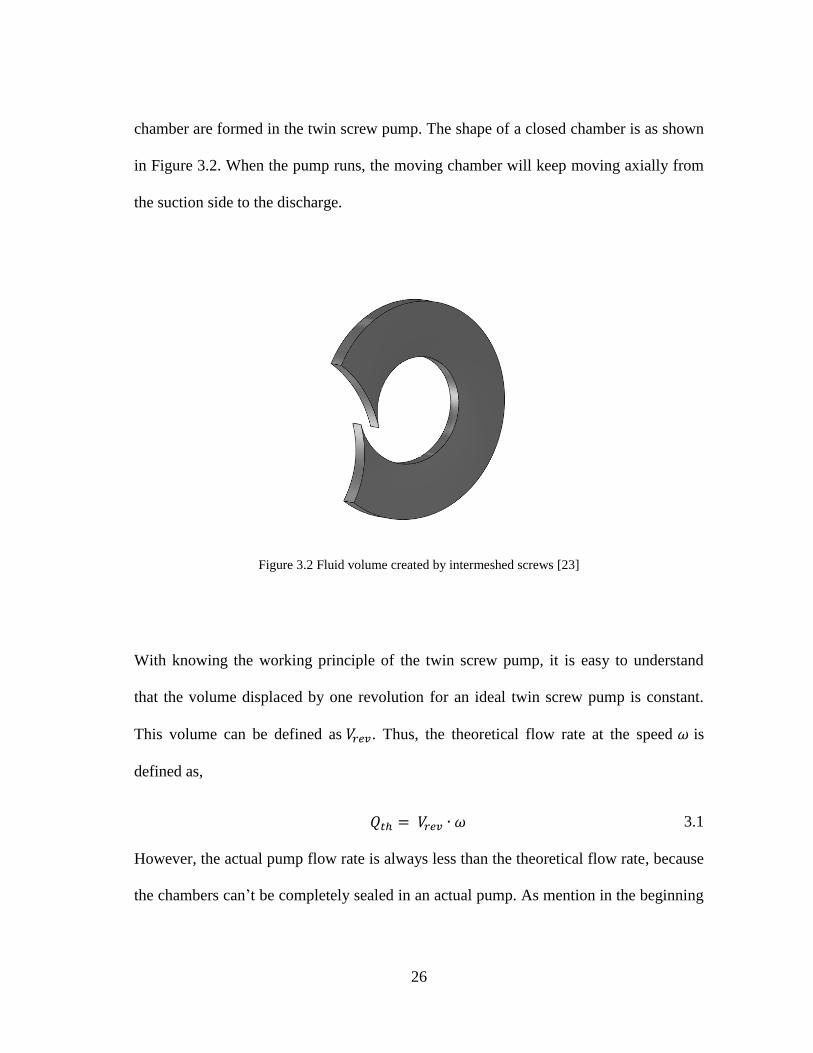
chamber are formed in the twin screw pump. The shape of a closed chamber is as shown
in Figure 3.2. When the pump runs, the moving chamber will keep moving axially from
the suction side to the discharge.
Figure 3.2 Fluid volume created by intermeshed screws [23]
With knowing the working principle of the twin screw pump, it is easy to understand
that the volume displaced by one revolution for an ideal twin screw pump is constant.
This volume can be defined as 𝑉𝑟𝑒𝑣. Thus, the theoretical flow rate at the speed 𝜔 is
defined as,
𝑄𝑡ℎ = 𝑉𝑟𝑒𝑣 ∙ 𝜔 3.1
However, the actual pump flow rate is always less than the theoretical flow rate, because
the chambers can’t be completely sealed in an actual pump. As mention in the beginning

27
of this chapter, there are clearances between the screws to avoid the wearing.
Additionally, there are also clearances existed between the screws and the housings.
These clearances are designed to promote the pump’s life. However, they also lead to the
degradation of the pump performance. Since they cause the leakage flow in the pump,
which decreases the pump’s actual flow rate. Especially with a high pressure rise, the
pump flow rate capacity can decrease severely. Thus, the actual flow rate of the twin
screw pump is the difference from the theoretical flow rate and the leakage flow rate.
The actual flow rate is subject to operation conditions.
3.2 Volumetric Efficiency
The existence of internal clearances leads to the degradation of volumetric flow rate
capacity of the twin screw pump. There are 3 types of clearances in the twin screw
pump, circumferential clearance (CC), radial clearance (RC) and flank clearance (FC),
which are detailed in Figure 3.3. The circumferential clearance is located between the
periphery of the screws and the housing, while the radial clearance is located between
the outer diameter of one rotor and the root diameter of the other rotor. The flank
clearance is formed by two adjacent flanks. Previous researches show that the
circumferential clearance accounts for about 80% of total leakage, while the radial
clearance and the flank clearance account for 20% of total leakage. Hence, the
circumferential clearance is the most important factor for the backflow.

28
Figure 3.3 Clearance types of the twin screw pumps [21]
The leakage flow rate varies with the clearances dimensions and pump working
conditions. Hence, the pump’s actual flow rate is also influenced by the clearances and
operating condition. The smaller clearances help to promote the pump’s flow rate
capacity, but it also leads to larger possibility of interior abrasion and friction loss.
What’s more, the actual flow rate is also subject to the pressure rise, GVF, fluid
viscosity, etc. To compare the pump actual flow rate capacity with its theoretical flow
rate capacity, it is necessary to define the parameter, volumetric efficiency ( 𝜂𝑣 ).
Volumetric efficiency is defined by the ratio of the actual volumetric flow rate to the
theoretical flow rate of the pump.
𝜂𝑣 =
𝑄𝑎
𝑄𝑡ℎ 3.2
Where 𝑄𝑎 represents the actual flow rate of the pump and 𝑄𝑡ℎ is the theoretical flow rate
of the pump. For the pump designer, it is a common goal to improve the pump’s
volumetric efficiency. Generally, increasing the pitch number is an effective method to

29
improve the volumetric efficiency. With more seals in the pump, the leakage flow will
decrease. It is found that the volumetric efficiency can drop severely when the pump
works at high GVF. In this case, it is necessary to introduce the sealflush recirculation.
According to the research of Patil, the optimum sealflush recirculation to obtain the best
volumetric efficiency is around 3% of the total flow rate.
3.3 Mechanical Efficiency
Mechanical Efficiency (𝜂𝑚𝑒𝑐ℎis defined as the ratio of the power delivered to the fluid
during the compression process to the power from the motor into the pump.
𝜂𝑚𝑒𝑐ℎ =
𝑃𝑛𝑒𝑡
𝑃𝑑𝑟𝑖𝑣𝑒 3.3
It represents friction losses incurred due to viscous and turbulence effect in the cavities
as well as different clearances, mechanical losses due to friction inside bearings, seals,
and gears.
The power transferred to the working fluid can be divided into two parts, the liquid
power (𝑃𝑙) and the gas power (𝑃𝑔). As a result,
𝑃𝑛𝑒𝑡 = 𝑃𝑙 + 𝑃𝑔 3.4
The 𝑃𝑙 is the power transferred to the liquid. It can be calculated with the following
equation,
𝑃𝑙 = 𝑄𝑙∆𝑝 3.5

30
When the twin screw pump runs at low GVF conditions, the temperature rise of the fluid
is small. Thus the process can be considered as isothermal. Then the power delivered to
the fluid can be calculated as:
𝑃𝑛𝑒𝑡, 𝑖𝑠𝑜𝑡ℎ𝑒𝑟𝑚𝑎𝑙 = 𝑄𝑙∆𝑝 + 𝑄𝑔𝑝𝑖𝑛ln (
𝑝𝑜𝑢𝑡
𝑝𝑖𝑛) 3.6
When a twin screw pump runs at high GVF conditions, the temperature rise is
significant. Polytropic compression process is applied to calculate the power delivered
into fluid.
𝑃𝑛𝑒𝑡, 𝑝𝑜𝑙𝑦𝑡𝑟𝑜𝑝𝑖𝑐 = 𝑄𝑙∆𝑝 +𝑛
𝑛 − 1𝑄𝑔𝑝𝑖𝑛 [(
𝑝𝑜𝑢𝑡
𝑝𝑖𝑛)
𝑛−1𝑛
− 1] 3.7
Where n is the polytropic constant. The value of n can be obtained knowing the inlet and
exit pressures and temperatures from the following equation,
𝑛 =𝐼𝑛 (
𝑝𝑖𝑛
𝑝𝑜𝑢𝑡)
𝐼𝑛 (𝑝𝑖𝑛
𝑝𝑜𝑢𝑡∙
𝑇𝑜𝑢𝑡
𝑇𝑖𝑛) 3.8
The polytropic constant varies from 1 to 𝑐𝑝
𝑐𝑣 in the compression process. The polytropic
constant equals to 𝑐𝑝
𝑐𝑣 when the compression process is adiabatic.
3.4 Pump Effectiveness
Pump effectiveness (𝜂𝑒𝑓𝑓) represents the ratio of power imparted into the multiphase
fluid to the power imparted into single liquid phase with same flow rate. [27] The pump
effectiveness can be calculated as the following equation,

31
𝜂𝑒𝑓𝑓 =
𝑃𝑛𝑒𝑡
𝑃ℎ𝑦𝑑𝑟𝑎𝑢𝑙𝑖𝑐 3.3
Where 𝑃𝑛𝑒𝑡 = 𝑃𝑛𝑒𝑡, 𝑖𝑠𝑜𝑡ℎ𝑒𝑟𝑚𝑎𝑙 or 𝑃𝑛𝑒𝑡, 𝑝𝑜𝑙𝑦𝑡𝑟𝑜𝑝𝑖𝑐 . The 𝑃ℎ𝑦𝑑𝑟𝑎𝑢𝑙𝑖𝑐 represents the power
imparted into working fluid if the flow is incompressible. It is calculated by the equation
below,
𝑃ℎ𝑦𝑑𝑟𝑎𝑢𝑙𝑖𝑐 = (𝑄𝑔 + 𝑄𝑙) ∙ 𝛥𝑝 3.4
The pump effectiveness indicates the pump ability to compress the multiphase flow.
Pump effectiveness decreases with an increase of the GVF.
In this chapter, the internal construction of the twin screw pump is highlighted. Essential
parameters to evaluate the twin screw pump performance are introduced. In the
following section, the experiment method will be presented. The test rig will also be
detailed.
32
4 METHODOLOGY
This chapter highlights the establishment of the test rig and the details of the
instruments. The pump was tested at the Turbomachinery Laboratory at Texas A&M
University. The facilities at the Turbomachinery Lab make it very convenient to set up
the test rig. Previous work generally chose water and air as the working fluids in the
experiment. However, the fluid in the oil well is usually the mixture of water, oil and
gas. To simulate the real working condition, the pump was tested with different working
fluids. Water and oil are selected as the working liquid to test the pump with different
water cuts: 100%, 80%, 50% and 0%. The compressed air was used as working gas to
perform the multiphase test with 100% water cut, while nitrogen was chosen for the oil
tests for safety. The water-air test was performed during August 2014, while the oil-
water-nitrogen test was performed during April 2015.
4.1 Experimental Set Up
4.1.1 Test Rigs
Figure 4.1 illustrates the P&ID diagram for the water-air test. The water test was
performed with an open loop. Only the liquid was recirculated in the test loop. Water
was boosted into the flow loop by a charge pump. Pressure was held at 120 psig with a
back pressure regulator. A water filter was installed in the water line to keep the water
into the pump clean. Compressed air was supplied by oil free screw compressors with a
common reservoir. The water and air flow rate was adjusted by the electro-pneumatic

33
valves and measured by the turbine flow meters. During the operation, the air was used
to control the pump inlet pressure at 100 psig by adjusting an electro-pneumatic valve.
The changing of GVF was accomplished by adjusting the water flow rate.
Figure 4.1 Flow loop diagram of water test
There are a series of water and air flow meters used to cover different flow ranges. Every
flow meter has different working range. During the test, the proper flow meter was
selected according to the water and air flow rate. Water and air were mixed in an intake
manifold before the pump inlet. Pressure transducers and thermocouples were installed
at the inlet and the exit of every stage. Three accelerometers were installed at the front,
the middle and the rear of the pump to monitor the vibration level during operation.
34
At the discharge of the pump, a pressure relief valve was applied to ensure the safe
operation of the pump. The control valve at the pump outlet was used to adjust the
discharge pressure of the pump. The valve was controlled by 4-20 mA current.
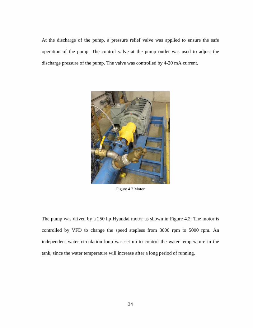
Figure 4.2 Motor
The pump was driven by a 250 hp Hyundai motor as shown in Figure 4.2. The motor is
controlled by VFD to change the speed stepless from 3000 rpm to 5000 rpm. An
independent water circulation loop was set up to control the water temperature in the
tank, since the water temperature will increase after a long period of running.
35
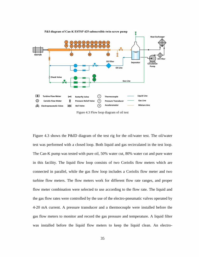
Figure 4.3 Flow loop diagram of oil test
Figure 4.3 shows the P&ID diagram of the test rig for the oil/water test. The oil/water
test was performed with a closed loop. Both liquid and gas recirculated in the test loop.
The Can-K pump was tested with pure oil, 50% water cut, 80% water cut and pure water
in this facility. The liquid flow loop consists of two Coriolis flow meters which are
connected in parallel, while the gas flow loop includes a Coriolis flow meter and two
turbine flow meters. The flow meters work for different flow rate ranges, and proper
flow meter combination were selected to use according to the flow rate. The liquid and
the gas flow rates were controlled by the use of the electro-pneumatic valves operated by
4-20 mA current. A pressure transducer and a thermocouple were installed before the
gas flow meters to monitor and record the gas pressure and temperature. A liquid filter
was installed before the liquid flow meters to keep the liquid clean. An electro-
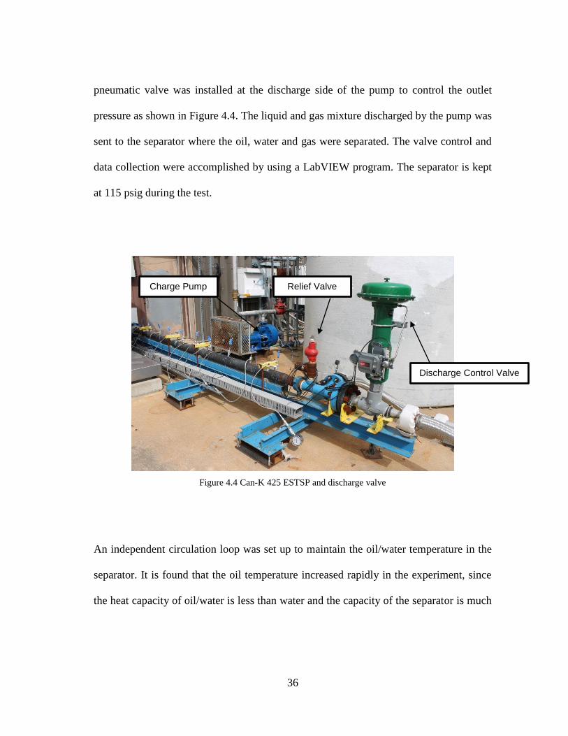
36
pneumatic valve was installed at the discharge side of the pump to control the outlet
pressure as shown in Figure 4.4. The liquid and gas mixture discharged by the pump was
sent to the separator where the oil, water and gas were separated. The valve control and
data collection were accomplished by using a LabVIEW program. The separator is kept
at 115 psig during the test.
Figure 4.4 Can-K 425 ESTSP and discharge valve
An independent circulation loop was set up to maintain the oil/water temperature in the
separator. It is found that the oil temperature increased rapidly in the experiment, since
the heat capacity of oil/water is less than water and the capacity of the separator is much
Charge Pump
Discharge Control Valve
Relief Valve

37
smaller than the water tank. The oil/water temperature is controlled by the heat
exchanger. Figure 4.5 shows the water tank, the heat exchangers and the separator.
Figure 4.5 Water tank, heat exchanger and separator
The Can-K pump is 29 feet long, with the diameter 4.25 inches. The Can-K pump was
coupled with the motor by a Lovejoy coupling. The pump-motor assembly is installed on
the test bench as shown in Figure 4.6. The front part of the pump is timing gears, thrust
module and centralizer. The pumping elements are located at the rear. There are 10
stages of pump modules in total.
Water Tank Separator
Heat Exchanger
Heat Exchanger

38
Figure 4.6 Pump and motor assembly (Klayton, 2013)
4.1.2 Instrumentations
Solid state pressure transducer of Omega PX-429 series were used to measure the
pressure. Detailed information of the pressure transducers are shown in Table 4.1. The
pressure transducer was connected with a resistance and a 20V power supply. The
resistance of the pressure transducer varied with the measured pressure. The pressure can
be calculated by measuring the voltage on the pressure transducer.
T-type thermocouples from Omega were used to measure the temperature. They were
integrated into data acquisition system with NI 9213. The accuracy of the thermocouple
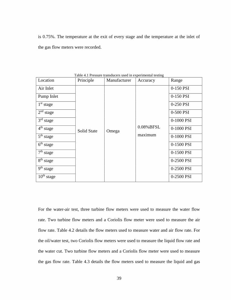
39
is 0.75%. The temperature at the exit of every stage and the temperature at the inlet of
the gas flow meters were recorded.
Table 4.1 Pressure transducers used in experimental testing
Location Principle Manufacturer Accuracy Range
Air Inlet
Solid State Omega 0.08%BFSL
maximum
0-150 PSI
Pump Inlet 0-150 PSI
1st stage 0-250 PSI
2nd stage 0-500 PSI
3rd stage 0-1000 PSI
4th stage 0-1000 PSI
5th stage 0-1000 PSI
6th stage 0-1500 PSI
7th stage 0-1500 PSI
8th stage 0-2500 PSI
9th stage 0-2500 PSI
10th stage 0-2500 PSI
For the water-air test, three turbine flow meters were used to measure the water flow
rate. Two turbine flow meters and a Coriolis flow meter were used to measure the air
flow rate. Table 4.2 details the flow meters used to measure water and air flow rate. For
the oil/water test, two Coriolis flow meters were used to measure the liquid flow rate and
the water cut. Two turbine flow meters and a Coriolis flow meter were used to measure
the gas flow rate. Table 4.3 details the flow meters used to measure the liquid and gas
40
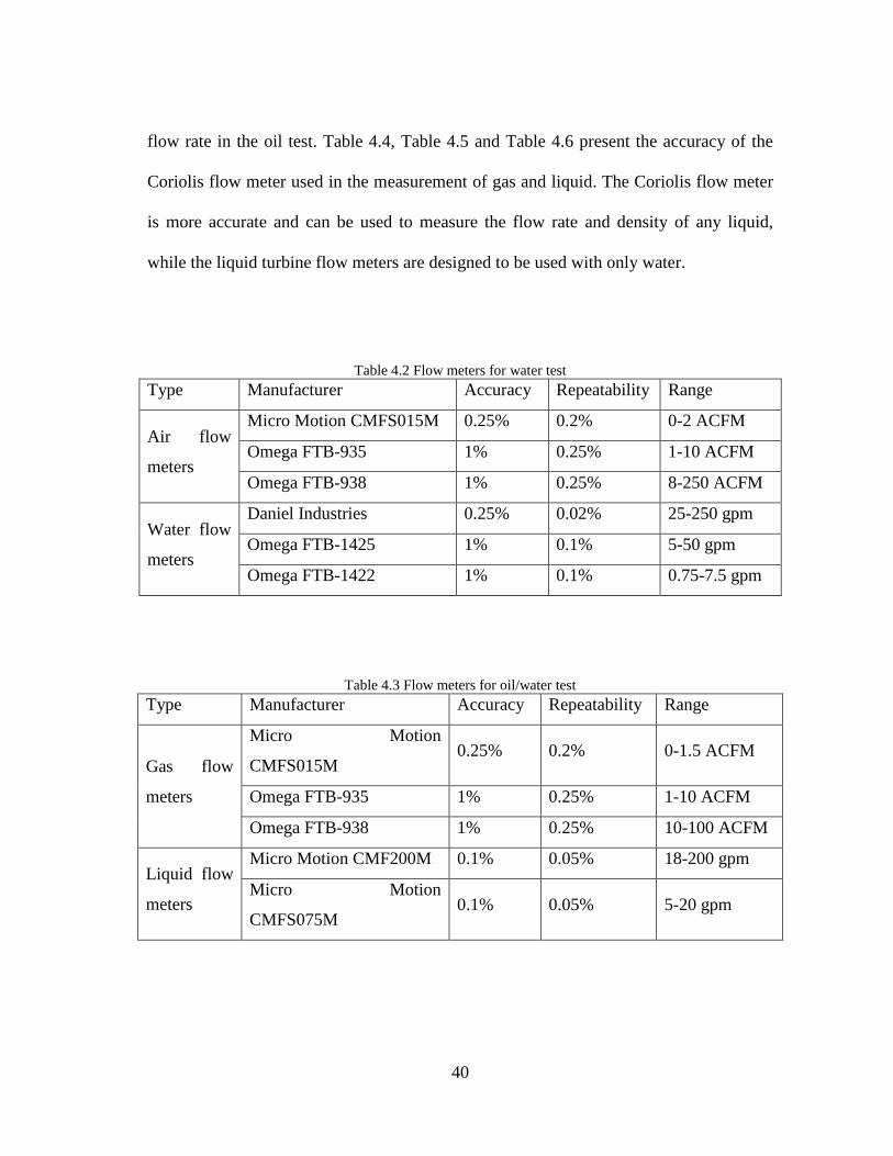
flow rate in the oil test. Table 4.4, Table 4.5 and Table 4.6 present the accuracy of the
Coriolis flow meter used in the measurement of gas and liquid. The Coriolis flow meter
is more accurate and can be used to measure the flow rate and density of any liquid,
while the liquid turbine flow meters are designed to be used with only water.
Table 4.2 Flow meters for water test
Type Manufacturer Accuracy Repeatability Range
Air flow
meters
Micro Motion CMFS015M 0.25% 0.2% 0-2 ACFM
Omega FTB-935 1% 0.25% 1-10 ACFM
Omega FTB-938 1% 0.25% 8-250 ACFM
Water flow
meters
Daniel Industries 0.25% 0.02% 25-250 gpm
Omega FTB-1425 1% 0.1% 5-50 gpm
Omega FTB-1422 1% 0.1% 0.75-7.5 gpm
Table 4.3 Flow meters for oil/water test
Type Manufacturer Accuracy Repeatability Range
Gas flow
meters
Micro Motion
CMFS015M 0.25% 0.2% 0-1.5 ACFM
Omega FTB-935 1% 0.25% 1-10 ACFM
Omega FTB-938 1% 0.25% 10-100 ACFM
Liquid flow
meters
Micro Motion CMF200M 0.1% 0.05% 18-200 gpm
Micro Motion
CMFS075M 0.1% 0.05% 5-20 gpm

41
Table 4.4 Micro Motion CMFS015M accuracy and repeatability (Gas)
Performance Specification Accuracy Repeatability
Mass flow rate 0.25% 0.2%
Temperature 1% 0.25%
Table 4.5 Micro Motion CMFS075M accuracy and repeatability (Liquid)
Performance Specification Accuracy Repeatability
Mass/volume flow rate 0.1% 0.05%
Density 0.5 kg/m3 0.2 kg/m3
Temperature 0.5% 0.2 °C
Table 4.6 Micro Motion CMF200M accuracy and repeatability (Liquid)
Performance Specification Accuracy Repeatability
Mass/volume flow rate 0.1% 0.05%
Density 0.5 kg/m3 0.2 kg/m3
Temperature 0.5% 0.2 °C
A TOSHIBA P9 adjustable speed drive (ASD) was used to control the motor’s speed.
The output power and output current of the ASD were automatically recorded by the
data acquisition system. The adjustment of motor’s speed during the test was
accomplished by the P9 ASD Electronic Operator Interface. A Hyundai motor was
installed to drive the pump, which can be operated continuously from 3000 RPM to 5000
RPM providing a maximum 250 HP power.
42
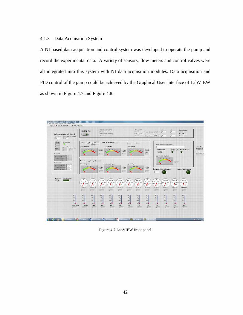
4.1.3 Data Acquisition System
A NI-based data acquisition and control system was developed to operate the pump and
record the experimental data. A variety of sensors, flow meters and control valves were
all integrated into this system with NI data acquisition modules. Data acquisition and
PID control of the pump could be achieved by the Graphical User Interface of LabVIEW
as shown in Figure 4.7 and Figure 4.8.
Figure 4.7 LabVIEW front panel

43
Figure 4.8 LabVIEW front panel (continue)
NI Module 9205 was used to collect data of pressure transducers, Coriolis flow meters,
and VFD. NI Module 9213 was used to collect data of thermocouples. Module 9265 was
used to control electro-pneumatic valves with 4-20 mA current. NI Module 9205 and
9213 were integrated with NI 9074 chassis which transmitted the signals to the computer
program. The output data of the turbine flow meters are transmitted by three iServer
Microservers from OMEGA. The specifications of the NI Modules and iServer are
shown in Table 4.7.
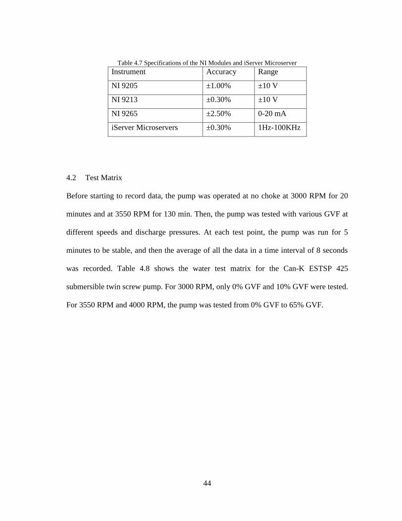
44
Table 4.7 Specifications of the NI Modules and iServer Microserver
Instrument Accuracy Range
NI 9205 ±1.00% ±10 V
NI 9213 ±0.30% ±10 V
NI 9265 ±2.50% 0-20 mA
iServer Microservers ±0.30% 1Hz-100KHz
4.2 Test Matrix
Before starting to record data, the pump was operated at no choke at 3000 RPM for 20
minutes and at 3550 RPM for 130 min. Then, the pump was tested with various GVF at
different speeds and discharge pressures. At each test point, the pump was run for 5
minutes to be stable, and then the average of all the data in a time interval of 8 seconds
was recorded. Table 4.8 shows the water test matrix for the Can-K ESTSP 425
submersible twin screw pump. For 3000 RPM, only 0% GVF and 10% GVF were tested.
For 3550 RPM and 4000 RPM, the pump was tested from 0% GVF to 65% GVF.
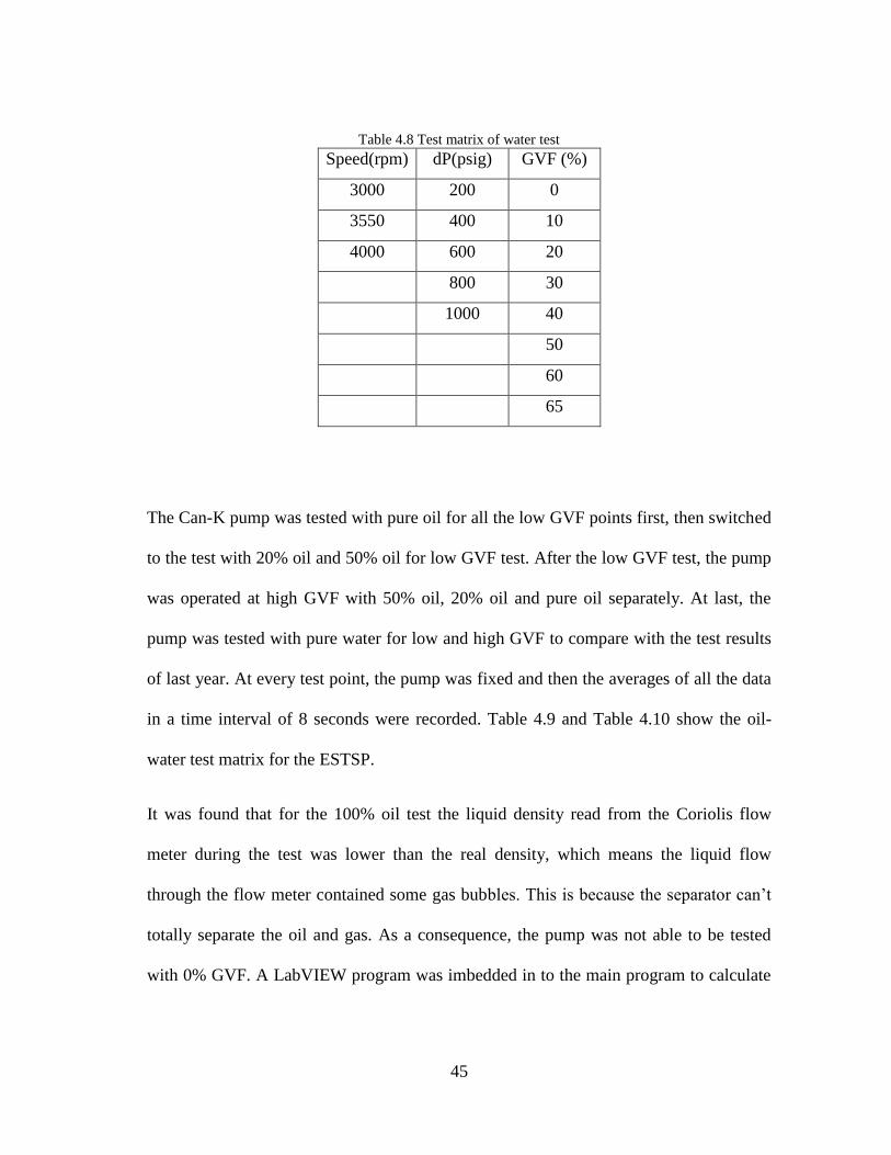
45
Table 4.8 Test matrix of water test
Speed(rpm) dP(psig) GVF (%)
3000 200 0
3550 400 10
4000 600 20
800 30
1000 40
50
60
65
The Can-K pump was tested with pure oil for all the low GVF points first, then switched
to the test with 20% oil and 50% oil for low GVF test. After the low GVF test, the pump
was operated at high GVF with 50% oil, 20% oil and pure oil separately. At last, the
pump was tested with pure water for low and high GVF to compare with the test results
of last year. At every test point, the pump was fixed and then the averages of all the data
in a time interval of 8 seconds were recorded. Table 4.9 and Table 4.10 show the oil-
water test matrix for the ESTSP.
It was found that for the 100% oil test the liquid density read from the Coriolis flow
meter during the test was lower than the real density, which means the liquid flow
through the flow meter contained some gas bubbles. This is because the separator can’t
totally separate the oil and gas. As a consequence, the pump was not able to be tested
with 0% GVF. A LabVIEW program was imbedded in to the main program to calculate
46
the correct GVF in the pump inlet considering the effect of the gas bubbles in the liquid
flow.
Table 4.9 Test matrix of oil test, low GVF
Oil Speed(rpm) dP(psig) GVF (%)
100 3000 100 10
50 3550 200 20
20 4000 400 30
600 40
800 50
1000 60
70
Table 4.10 Test matrix of oil test, high GVF
Oil Speed(rpm) dP(psig) GVF (%)
100 3550 100 75
50 4000 200 80
20 400 85
For 3000 RPM, only 10% GVF was tested. For 3550 RPM and 4000 RPM, the pump
was tested from 10% GVF to 70% GVF.
In this chapter, the test rig and the instruments are detailed. Test method and the
experiment content are also presented. In the next chapter, the test results will be

47
presented. The pump performance will be analyzed and compared with that of the
double-end pump.

48
5 PERFORMANCE EVALUATION OF EXPERIMENTAL RESULTS
This chapter will discuss the experimental results. First, the multiphase performance of
the Can-K pump will be presented and discussed. Experimental results of water test, oil
test and water/oil test are analyzed. Then, the performance of the Can-K pump will be
compared with that of the single-stage twin screw pump. In this study, the test data of a
Colfax pump is selected to make the comparison.
The Can-K pump was tested with 100% water cut twice, the first time was tested with
the open loop in Aug. 2014 and the second time was tested with the closed loop in Apr.
2015. The water test data of the Apr. 2015 is selected to evaluate the pump performance
in the discussion. The two sets of 100% water cut test data are compared in this chapter
as well.
5.1 Power Consumption
Power consumption is defined as the power required by the motor to maintain the pump
speed. The power transferred to motor was recorded by the LabVIEW program for each
test point.
Figure 5.1 shows the variation of power consumption of the 100% water cut test with
different differential pressures at 10% GVF. Power consumption increases nearly
linearly as the differential pressure increases. Power consumption generally can be
divided into two components, one component is to pressurize the working fluid and
another component is to overcome the viscous and friction losses in the pump. The
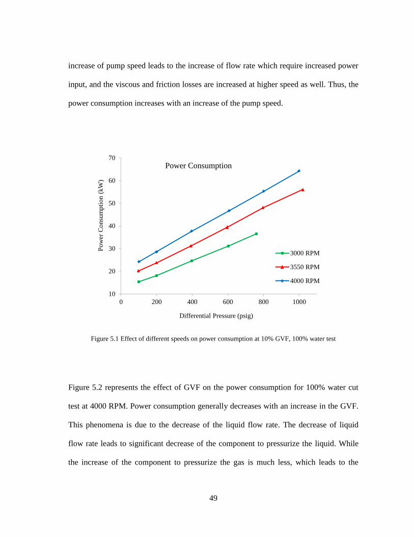
49
increase of pump speed leads to the increase of flow rate which require increased power
input, and the viscous and friction losses are increased at higher speed as well. Thus, the
power consumption increases with an increase of the pump speed.
Figure 5.1 Effect of different speeds on power consumption at 10% GVF, 100% water test
Figure 5.2 represents the effect of GVF on the power consumption for 100% water cut
test at 4000 RPM. Power consumption generally decreases with an increase in the GVF.
This phenomena is due to the decrease of the liquid flow rate. The decrease of liquid
flow rate leads to significant decrease of the component to pressurize the liquid. While
the increase of the component to pressurize the gas is much less, which leads to the
10
20
30
40
50
60
70
0 200 400 600 800 1000
Po
wer
Co
nsu
mp
tio
n (
kW
)
Differential Pressure (psig)
Power Consumption
3000 RPM
3550 RPM
4000 RPM
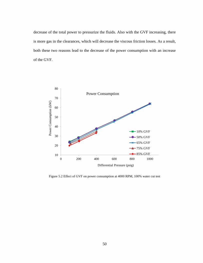
50
decrease of the total power to pressurize the fluids. Also with the GVF increasing, there
is more gas in the clearances, which will decrease the viscous friction losses. As a result,
both these two reasons lead to the decrease of the power consumption with an increase
of the GVF.
Figure 5.2 Effect of GVF on power consumption at 4000 RPM, 100% water cut test
10
20
30
40
50
60
70
80
0 200 400 600 800 1000
Po
wer
Co
nsu
mp
tio
n (
kW
)
Differential Pressure (psig)
Power Consumption
10% GVF
50% GVF
65% GVF
75% GVF
85% GVF

51
Figure 5.3 Effect of GVF on power consumption at 4000 RPM, 100% water cut test
As shown in Figure 5.3, the larger pump head leads to larger power consumption. With
the same power consumption, the pump head increases with an increase of the GVF.
This is because the density of the working fluid decreases with an increase of the GVF.
Thus, the same power consumption can produce a larger pump head.
Water cut has an essential influence on the power consumption as well. As shown in
Figure 5.4, the power consumption decreases with the increase of water cut. The
viscosity of the working fluid decrease with the increase of water cut. The friction
losses generally increase with the viscosity. However, in this study, the oil viscosity is
about 2 ct, which is very close with that of water. Thus, the effect of viscosity isn’t the
10
20
30
40
50
60
70
80
0 1000 2000 3000 4000 5000 6000 7000 8000
Po
wer
Co
nsu
mp
tio
n (
kW
)
Head (ft)
Power vs. Head
10% GVF
30% GVF
50% GVF
65% GVF
85% GVF

52
dominant factor. In this research, the 100% water test shows the largest total flow rate
capacity. According to equation 3.4, the higher flow rate requires more power to
pressurize the fluid. The increase of power imparted into the fluid counteracts the
decrease of power to overcome the friction losses. As a consequence, the power
consumption increase with water cut.
Figure 5.4 Effect of water cut on power consumption at 4000 RPM, 10% GVF
5.2 Pressure and Temperature Distribution
In this research, pressure and temperature at the end of each stage are measured for each
test point. Pressure and temperature recorded is the mean value within a time period of 8
seconds, since the pressure and the temperature kept changing during the experiment.
20
25
30
35
40
45
50
55
60
65
70
0 200 400 600 800 1000
Po
wer
Co
nsu
mp
tio
n (
kW
)
Differential Pressure (psig)
Power Consumption
100% water cut
80% water cut
50% water cut
0% water cut

53
The pressure and temperature distributions help to understand the compression process
of the working fluid in the pump.
Figure 5.5 shows the pressure distribution stage by stage along the pump at 4000 RPM
for 100% water cut test. The pressure transducers are located at the inlet and the outlet of
every stage. Using the pressure distribution it is convenient to find the pressure rise cross
a certain stage. The pressure distribution is affected by the GVF of the working fluid. As
shown in Figure 5.6, at the low GVFs, the shape of the pressure distribution is concave-
down. However, with an increase of the GVF, the shape of the pressure distribution
changes to concave-up. The pressure changes the largest at the last stage.
Figure 5.5 Pressure distributions at 4000 RPM, 100% water cut, 10% GVF
0
200
400
600
800
1000
1200
0 1 2 3 4 5 6 7 8 9 10
Pre
ssure
(p
sig)
Position, Inlet to Exit
Pressure Distribution100 psig dP
200 psig dP
400 psig dP
600 psig dP
800 psig dP
1000 psig dP

54
Figure 5.6 Effect of GVF on pressure distribution at 4000 RPM, 100% water cut, 400 psig differential
pressure
The temperature distribution along the pump is shown in Figure 5.7. Due to the viscous
friction and the compression processes in the pump, the temperature rises from the
suction side to the discharge side. Since the heat capacity of the liquid is much larger
than that of the gas, the temperature rise is very small at the low GVFs. In this condition,
the compression process is close to isothermal process. However, with the increase of
GVF, there is insufficient liquid in the pump to absorb the heat produced by internal
frictions and compression process. As a result, the temperature rise increases with the
increase of GVF. In consequence, the compression process can be considered as
polytropic process at the extremely high GVF conditions. The variation of temperature
50
100
150
200
250
300
350
400
450
500
550
0 1 2 3 4 5 6 7 8 9 10
Pre
ssure
(p
sig)
Position, Inlet to Exit
Pressure Distribution10% GVF
30% GVF
50% GVF
65% GVF
85% GVF
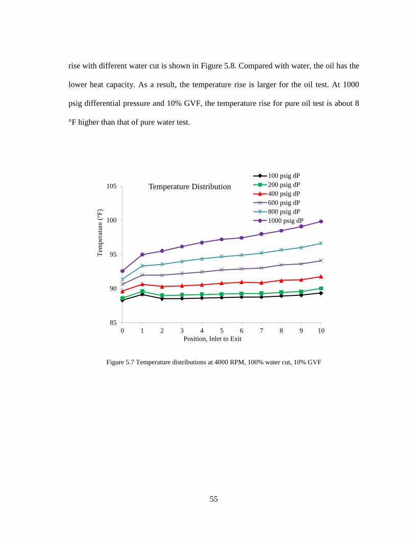
55
rise with different water cut is shown in Figure 5.8. Compared with water, the oil has the
lower heat capacity. As a result, the temperature rise is larger for the oil test. At 1000
psig differential pressure and 10% GVF, the temperature rise for pure oil test is about 8
°F higher than that of pure water test.
Figure 5.7 Temperature distributions at 4000 RPM, 100% water cut, 10% GVF
85
90
95
100
105
0 1 2 3 4 5 6 7 8 9 10
Tem
per
ature
(°F
)
Position, Inlet to Exit
Temperature Distribution
100 psig dP
200 psig dP
400 psig dP
600 psig dP
800 psig dP
1000 psig dP

56
Figure 5.8 Effect of water cut on total temperature rise at 4000 RPM, 10% GVF
The polytropic coefficient is an essential parameter to indicate the compression process
in the twin screw pump. In the compression process, the polytropic coefficient varies
from 1 to 𝑐𝑝
𝑐𝑣, indicating the compression process varied from isothermal to adiabatic. As
shown in Figure 5.8, the polytropic coefficient in this research is around 1.0 even for
85% GVF. As a result, the compression process in this research is very close to
isothermal process.
0
2
4
6
8
10
12
14
16
0 200 400 600 800 1000
To
tal
Tem
per
ature
Ris
e (°
F)
Differential Pressure (psig)
Temperature Rise
100% water cut
0% water cut

57
Figure 5.9 Polytropic coefficient of different water cuts, 4000 RPM
Figure 5.10 shows the effect of water cut on the polytropic coefficient. Polytropic
coefficient of 0% water cut test is higher than that of 100% water cut test. This is
because the temperature rise of 0% water cut test is higher due to the lower heat capacity
of the oil. Compared with the 0% water cut test, thus the 100% water cut test is more
close to the isothermal process.
0.9
0.95
1
1.05
1.1
0 200 400 600 800 1000
Poly
trop
ic C
oef
fici
ent
Differential Pressure (psig)
100% water cut
10% GVF
30% GVF
50% GVF
70% GVF
85% GVF
0.9
0.95
1
1.05
1.1
0 200 400 600 800 1000
Poly
trop
ic C
oef
fici
ent
Differential Pressure (psig)
80% water cut
10% GVF
30% GVF
50% GVF
70% GVF
85% GVF
0.9
0.95
1
1.05
1.1
0 200 400 600 800 1000
Poly
trop
ic C
oef
fici
ent
Differential Pressure (psig)
50% water cut
10% GVF
30% GVF
50% GVF
70% GVF
85% GVF0.9
0.95
1
1.05
1.1
0 200 400 600 800 1000
Poly
trop
ic C
oef
fici
ent
Differential Pressure (psig)
0% water cut
10% GVF
30% GVF
50% GVF
70% GVF
85% GVF

58
Figure 5.10 Effect of water cut on polytropic coefficient at 4000 RPM, 20% GVF
5.3 Volumetric Flow Rate Capacity
Volumetric flow rate capacity refers to the total flow rate flowing into the pump inlet. As
mentioned in the previous section, theoretical flow rate capacity of the twin screw pump
is only a function of geometrical parameters and pump speed. However, the actual
volumetric flow rate capacity is affected by various factors, such as differential pressure,
GVF, viscosity, et al. In this section, the characteristics of total flow rate capacity of the
Can-K pump will be investigated.
Figure 5.11 shows the volumetric flow rate capacity at 3550 RPM and 4000 RPM with
different GVF. At 4000 RPM, the theoretical volumetric flow rate is 113.5 gpm. But the
0.995
0.997
0.999
1.001
1.003
1.005
1.007
1.009
1.011
1.013
1.015
0 200 400 600 800 1000
Po
lytr
op
ic C
oef
fici
ent
Differential Pressure (psig)
Polytropic Coefficient
100% water cut
0% water cut

59
actual flow rate capacity is less than the theoretical flow rate due to the internal leakages.
The actual flow rate capacity varies with differential pressure and GVF. As shown in
Figure 5.11, the volumetric flow rate decreases with the increase of differential pressure.
With the increase of differential pressure, there is more leakage flow from discharge side
back to suction side. Thus, the total flow rate entering pump inlet is decreased. It is also
found that the volumetric flow rate increases with an increase of the GVF at the same
differential pressure. As shown in Figure 5.12 and Figure 5.13, the volumetric flow rate
capacity becomes the largest at 85% GVF with the same differential pressure. The effect
of GVF on the volumetric flow rate has been researched previously. Both Patil [23] and
Kroupa [21] found that the volumetric flow rate capacity increases with GVF first then
decreases. Patil found that the maximum volumetric flow rate capacity occurs when the
pump operated at around 90% GVF. In this research, the pump was tested with the GVF
up to 85%. The total flow rate capacity keeps rising with the increase GVF. With more
gas injected into the clearance, the two phase flow performs the seal function. Since the
sonic velocity of the two phase flow decreases as the GVF increases, and then increases
as the GVF increases. Thus, the sonic velocity of the two phase flow is lower than that of
pure liquid or pure gas. As a result, the two phase flow is more inclined to be choked in
the clearance, which means the two phase flow is able to provide a better seal function.
Water cut shows an essential effect on the total flow rate. As shown in Figure 5.14, the
100% water test presents the largest total flow rate capacity. With the decrease of water
cut, there is a slight drop of total flow rate capacity, especially at high differential
pressures. Chan [6] investigated the effect of viscosity. For the pure-liquid test, it is

60
found that increase in viscosity leads to the decrease of leakage flow. While for the high
GVF operation, viscosity isn’t a dominant role to determine the total flow rate. Patil [23]
also found that total flow rate capacity decreases with the increase of viscosity at the
high GVFs, especially when the viscosity increases from 1 cp to 10 cp. Patil [23]
concluded that there is insufficient liquid to seal the gas in the clearance at the high GVF
conditions due to the decreased fluidity. In this research, it is found that flow rate
capacity decreases with the increase of viscosity for all GVFs. As shown in Figure 5.14,
the flow rate capacity of the water test is always higher than that of oil test.
Figure 5.11 Effect of pump speed on volumetric flow rate capacity at 10% GVF, 100% water cut test
10
20
30
40
50
60
70
80
90
0 200 400 600 800 1000
Vo
lum
etri
c F
low
Rat
e (g
pm
)
Differential Pressure (psig)
Volumetric flow rate capacity for Different Speeds
of 100% water test, 10% GVF
3000 RPM
3550 RPM
4000 RPM

61
Figure 5.12 Volumetric flow rate capacity at 4000 RPM, 100% water test
Figure 5.13 Volumetric flow rate capacity at 4000 RPM, pure oil test
0
10
20
30
40
50
60
70
80
90
100
0 200 400 600 800 1000
To
tal
Flo
w R
ate
(gp
m)
Differential Pressure (psig)
4000 RPM, 100% water cut test
10% GVF
20% GVF
30% GVF
40% GVF
50% GVF
60% GVF
70% GVF
75% GVF
80% GVF
85% GVF
0
10
20
30
40
50
60
70
80
90
100
0 200 400 600 800 1000
To
tal
Flo
w R
ate
(gp
m)
Differential Pressure (psig)
4000 RPM, 0% water cut test
10% GVF
20% GVF
30% GVF
40% GVF
50% GVF
60% GVF
70% GVF
75% GVF
80% GVF
85% GVF

62
Figure 5.14 Effect of water cut on volumetric flow rate capacity
5.4 Volumetric Efficiency
Volumetric efficiency indicates the ratio of actual flow rate capacity to theoretical flow
rate capacity. Figure 5.15 shows the variation of volumetric efficiency with different
GVF at 4000 RPM for 100% water cut test. Figure 5.16 shows the variation of
volumetric efficiency with different GVF at 4000 RPM for 100% oil test. Since the
30
35
40
45
50
55
60
65
70
75
80
0 200 400 600 800 1000
Tota
l F
low
Rat
e (g
pm
)
Differential Pressure (psig)
4000 RPM, 10% GVF
00% watercut
50% watercut
80% watercut
100% watercut
35
40
45
50
55
60
65
70
75
80
85
0 200 400 600 800 1000
Tota
l F
low
Rat
e (g
pm
)
Differential Pressure (psig)
4000 RPM, 30% GVF00% watercut
50% watercut
80% watercut
100% watercut
45
50
55
60
65
70
75
80
85
90
0 200 400 600 800 1000
Tota
l F
low
Rat
e (g
pm
)
Differential Pressure (psig)
4000 RPM, 50% GVF
00% watercut
50% watercut
80% watercut
100% watercut
55
60
65
70
75
80
85
90
95
0 200 400 600 800 1000
Tota
l F
low
Rat
e (g
pm
)
Differential Pressure (psig)
4000 RPM, 70% GVF
00% watercut
50% watercut
80% watercut
100% watercut
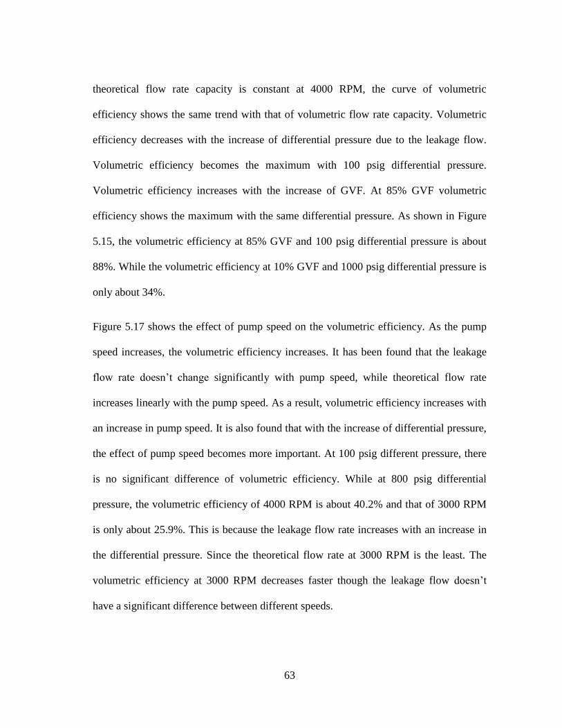
63
theoretical flow rate capacity is constant at 4000 RPM, the curve of volumetric
efficiency shows the same trend with that of volumetric flow rate capacity. Volumetric
efficiency decreases with the increase of differential pressure due to the leakage flow.
Volumetric efficiency becomes the maximum with 100 psig differential pressure.
Volumetric efficiency increases with the increase of GVF. At 85% GVF volumetric
efficiency shows the maximum with the same differential pressure. As shown in Figure
5.15, the volumetric efficiency at 85% GVF and 100 psig differential pressure is about
88%. While the volumetric efficiency at 10% GVF and 1000 psig differential pressure is
only about 34%.
Figure 5.17 shows the effect of pump speed on the volumetric efficiency. As the pump
speed increases, the volumetric efficiency increases. It has been found that the leakage
flow rate doesn’t change significantly with pump speed, while theoretical flow rate
increases linearly with the pump speed. As a result, volumetric efficiency increases with
an increase in pump speed. It is also found that with the increase of differential pressure,
the effect of pump speed becomes more important. At 100 psig different pressure, there
is no significant difference of volumetric efficiency. While at 800 psig differential
pressure, the volumetric efficiency of 4000 RPM is about 40.2% and that of 3000 RPM
is only about 25.9%. This is because the leakage flow rate increases with an increase in
the differential pressure. Since the theoretical flow rate at 3000 RPM is the least. The
volumetric efficiency at 3000 RPM decreases faster though the leakage flow doesn’t
have a significant difference between different speeds.

64
Figure 5.18 shows the effect of water cut on volumetric efficiency, which presents the
same trend with the curve of volumetric flow rate capacity. At the low differential
pressure, water cut has no evident effect on volumetric efficiency. With the increase of
differential pressure, 100% water cut test shows the highest volumetric efficiency.
Figure 5.15 Volumetric efficiency at 4000 RPM, 100% water cut test
0
0.1
0.2
0.3
0.4
0.5
0.6
0.7
0.8
0.9
1
0 200 400 600 800 1000
Vo
lum
etri
c E
ffic
iency
Differential Pressure (psig)
4000 RPM, 100% water cut test
10% GVF20% GVF30% GVF40% GVF50% GVF60% GVF70% GVF75% GVF80% GVF

65
Figure 5.16 Volumetric efficiency at 4000 RPM, 0% water cut test
Figure 5.17 Effect of speed on volumetric efficiency at 10% GVF, 100% Water Test
0
0.1
0.2
0.3
0.4
0.5
0.6
0.7
0.8
0.9
1
0 200 400 600 800 1000
Vo
lum
etri
c E
ffic
iency
Differential Pressure (psig)
4000 RPM, 0% water cut test
10% GVF
20% GVF
30% GVF
40% GVF
50% GVF
60% GVF
70% GVF
75% GVF
80% GVF
85% GVF
0
0.1
0.2
0.3
0.4
0.5
0.6
0.7
0.8
0.9
1
0 200 400 600 800 1000
Vo
lum
etri
c E
ffic
iency
Differential Pressure (psig)
Effect of pump speed on the volumetric efficiency
3000 RPM
3550 RPM
4000 RPM

66
Figure 5.18 Effect of water cut on volumetric efficiency at 4000 RPM, 10% GVF
5.5 Mechanical Efficiency
Mechanical efficiency indicates the ratio of the power delivered to the fluid to the power
transferred from the motor to the pump. As shown in Figure 5.9, the polytropic
coefficient is nearly equal to 1.0 at all test conditions, which means that the compression
is very close to an isothermal process.
0.2
0.3
0.4
0.5
0.6
0.7
0.8
0 200 400 600 800 1000
Vo
lum
etri
c E
ffic
iency
Differential Pressure (psig)
Effect of water cut on the volumetric efficiency
100% water cut
80% water cut
50% water cut
0% water cut

67
Figure 5.19 Mechanical efficiency (isothermal) for 100% water cut test at 4000 RPM
Figure 5.20 Mechanical efficiency (isothermal) for 0% water cut test at 4000 RPM
0
0.05
0.1
0.15
0.2
0.25
0.3
0 200 400 600 800 1000
Iso
ther
mal
Eff
icie
ncy
Differential Pressure (psig)
Mechanical Efficiency
10% GVF
30% GVF
50% GVF
65% GVF
85% GVF
0
0.05
0.1
0.15
0.2
0.25
0.3
0 200 400 600 800 1000
Iso
ther
mal
Eff
icie
ncy
Differential Pressure (psig)
Mechanical Efficiency
10% GVF
30% GVF
50% GVF
70% GVF
85% GVF

68
Figure 5.19 presents the mechanical efficiency of the 100% water test. Figure 5.20
presents the mechanical efficiency of the 100% oil test. With the increase of differential
pressure, mechanical efficiency increases first, and then decreases with the increase of
differential pressure.
Figure 5.21 Power imparted into liquid and gas at different GVF of 100% water cut test
0
2
4
6
8
10
12
14
16
18
20
0 500 1000
Pow
er i
mp
arte
d i
nto
Flu
id (
kW
)
Differential Pressure (psig)
10% GVFliquid, 3000 RPM
liquid, 3550 RPM
liquid, 4000 RPM
gas, 3000 RPM
gas, 3550 RPM
gas, 4000 RPM
0
2
4
6
8
10
12
14
16
18
20
0 500 1000
Pow
er i
mp
arte
d i
nto
Flu
id (
kW
)
Differential Pressure (psig)
50% GVFliquid, 3550 RPM
liquid, 4000 RPM
gas, 3550 RPM
gas, 4000 RPM
0
1
2
3
4
5
6
7
8
9
10
0 500 1000
Pow
er i
mp
arte
d i
nto
Flu
id (
kW
)
Differential Pressure (psig)
65% GVFliquid, 3550 RPM
liquid, 4000 RPM
gas, 3550 RPM
gas, 4000 RPM
0
1
2
3
4
5
6
7
8
9
10
0 100 200 300 400 500
Pow
er i
mp
arte
d i
nto
Flu
id (
kW
)
Differential Pressure (psig)
85% GVF
liquid, 3550 RPM
liquid, 4000 RPM
gas, 3550 RPM
gas, 4000 RPM

69
Figure 5.22 Friction losses of 100% water cut test
The power imparted into the pump can be divided into two components, one is to
pressurize the fluid and another one is to overcome the friction losses. To understand the
variation of mechanical efficiency, it is necessary to investigate the variation of the two
components at different operating conditions. Figure 5.21 shows the variation of power
imparted into liquid and gas at different operating conditions for the 100% water cut test.
Figure 5.22 illustrates the variation of power component to overcome the viscous and
friction losses. At the low differential pressure, the component to pressurize the fluid
increases rapidly with the increase of differential pressure. Thus, the mechanical
efficiency increases at the low differential pressure. At the high differential pressure, the
rapid decrease of flow rate leads to the decrease of the component to pressurize the fluid
0
5
10
15
20
25
30
35
40
45
50
0 200 400 600 800 1000
Fri
ctio
n L
oss
es (
kW
)
Differential Pressure (psig)
Friction Losses
10% GVF, 3000 RPM
10% GVF, 3550 RPM
10% GVF, 4000 RPM
50% GVF, 3550 RPM
50% GVF, 4000 RPM
65% GVF, 3550 RPM
65% GVF, 4000 RPM
85% GVF, 3550 RPM
85% GVF, 4000 RPM

70
while the component to overcome the friction losses increases rapidly. As a result, the
mechanical efficiency decreases at the high differential pressure.
With the differential pressure higher than 400 psig, mechanical efficiency decreases with
the increase of GVF. Figure 5.21 shows the variation of power imparted to the liquid and
the gas with different differential pressures. It is found that the power imparted in to the
liquid is dominant with the GVF up to 65%. Since compared with the power imparted
into the liquid and the power component to overcome the friction losses, the power
imparted into the gas is relatively small. However, the power imparted into the liquid
drops dramatically with the increase of GVF, which leads to the decrease of total power
imparted into the fluid. As mentioned in the previous section, the power consumption
changes little with the increase of GVF. Thus, the mechanical efficiency drops with the
increase of GVF.
As shown in Figure 5.23, the pump speed has an essential effect on the mechanical
efficiency. With the differential pressure less than 200 psig, the mechanical efficiency
doesn’t have big difference between different pump speeds. However, mechanical
efficiency increases with the increase of pump speed when differential pressure is larger
than 200 psig. As mentioned in the section of volumetric flow rate, volumetric flow rate
increases with the increase of pump speed. Thus, with the increase of pump speed, the
power imparted into the fluid increases faster than the power to overcome the fraction
losses. As a consequence, it shows higher mechanical efficiency at higher pump speed.

71
Figure 5.23 Effect of pump speed on mechanical efficiency (Isothermal) at 10% GVF, 100% water test
Figure 5.24 shows the effect of water cut on the mechanical efficiency. The mechanical
efficiency of different water cuts only shows the difference at the high differential
pressures. Since 100% water cut test shows the highest volumetric flow rate in this
research especially at high differential pressure, the power imparted into the fluid
increases with the increase of water cut. It is found the viscous and friction losses don’t
change much with different water cuts. As a result, the mechanical efficiency increases
with the increase of water cut.
0
0.05
0.1
0.15
0.2
0.25
0.3
0 200 400 600 800 1000
Iso
ther
mal
Eff
icie
ncy
Differential Pressure (psig)
Mechanical Efficiency
3000 RPM
3550 RPM
4000 RPM

72
Figure 5.24 Effect of water cut on mechanical efficiency at 4000 RPM, 10% GVF
5.6 Pump Effectiveness
Pump effectiveness reflects the pump ability to compress multiphase flow. Figure 5.25
and Figure 25 illustrates the effect of GVF on the pump effectiveness for 100% and 0%
water cut test. Pump effectiveness decreases with the increase of differential pressure.
With the increase of GVF, pump effectiveness decreases faster due to the increasing gas
fraction in the multiphase flow. Pump effectiveness decreases rapidly with the increase
of GVF.
0
0.05
0.1
0.15
0.2
0.25
0.3
0 200 400 600 800 1000
Mec
han
ical
Eff
icie
ncy
Differential Pressure (psig)
4000 RPM, 100% water cut test
100% water cut
80% water cut
50% water cut
0% water cut
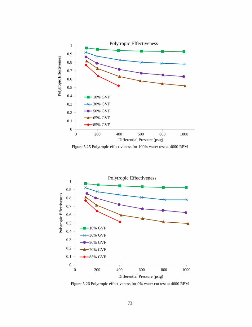
73
Figure 5.25 Polytropic effectiveness for 100% water test at 4000 RPM
Figure 5.26 Polytropic effectiveness for 0% water cut test at 4000 RPM
0
0.1
0.2
0.3
0.4
0.5
0.6
0.7
0.8
0.9
1
0 200 400 600 800 1000
Po
lytr
op
ic E
ffec
tiven
ess
Differential Pressure (psig)
Polytropic Effectiveness
10% GVF
30% GVF
50% GVF
65% GVF
85% GVF
0
0.1
0.2
0.3
0.4
0.5
0.6
0.7
0.8
0.9
1
0 200 400 600 800 1000
Po
lytr
op
ic E
ffec
tiven
ess
Differential Pressure (psig)
Polytropic Effectiveness
10% GVF
30% GVF
50% GVF
70% GVF
85% GVF

74
5.7 Leakage Flow Rate
As discussed in the previous section, the non-contact design of pump rotors results in the
existence of internal clearances in the pump. Due to the internal clearances, there is
leakage flow from discharge to inlet in the pump. Leakage flow rate is the difference of
the theoretical flow rate and the actual flow rate, which can be expressed as,
𝑄𝑙 = 𝑄𝑡ℎ − 𝑄𝑎 5.1
Where the actual flow rate, 𝑄𝑎, is the flow rate of fluid entering the inlet of the pump.
The leakage flow rate is generally a function of differential pressure, GVF, and pump
speed. It is influenced by the property of working fluid as well. In this research, the
leakage flow of the Can-K pump will be evaluated under different working conditions.
Pump speed has an important effect on the leakage flow rate. Figure 5.27 shows the
effect of pump speed on the leakage flow rate. It is found that as the pump speed
increases, the leakage flow rate increases at 10% GVF. However, with an increase of the
GVF the leakage flow rate is lower at 4000 RPM than that at 3550 RPM.
The leakage flow is typically composed by two components: one is due to the
differential pressure and one is due to the rotation,
𝑄𝑙 = 𝑄𝑑𝑃 + 𝑄𝑟 5.2

75
Figure 5.27 Effect of pump speed on leakage flow for 100% water cut test
0
10
20
30
40
50
60
70
80
90
100
0 200 400 600 800 1000
Lea
kag
e F
low
Rat
e (g
pm
)
Differential Pressure (psig)
10% GVF
3000 RPM
3550 RPM
4000 RPM
0
10
20
30
40
50
60
70
80
90
100
0 200 400 600 800 1000
Lea
kag
e F
low
Rat
e (g
pm
)
Differential Pressure (psig)
20% GVF
3550 RPM
4000 RPM
0
10
20
30
40
50
60
70
80
90
100
0 200 400 600 800 1000
Lea
kag
e F
low
Rat
e (g
pm
)
Differential Pressure (psig)
30% GVF
3550 RPM
4000 RPM
0
10
20
30
40
50
60
70
80
90
100
0 200 400 600 800 1000
Lea
kag
e F
low
Rat
e (g
pm
)
Differential Pressure (psig)
40% GVF
3550 RPM
4000 RPM
0
10
20
30
40
50
60
70
80
90
100
0 200 400 600 800 1000
Lea
kag
e F
low
Rat
e (g
pm
)
Differential Pressure (psig)
50% GVF
3550 RPM
4000 RPM
0
10
20
30
40
50
60
70
80
90
100
0 200 400 600 800 1000
Lea
kag
e F
low
Rat
e (g
pm
)
Differential Pressure (psig)
65% GVF
3550 RPM
4000 RPM

76
As the pump speed increases with constant differential pressure, the leakage flow of
differential pressure component remains the same, while the rotation component
increases with the increase of pump speed at the low GVF conditions. At the low GVF
conditions, the rotation component increases with the increasing pump speed. However,
with an increase of the GVF, the effect of centrifugal effect becomes the dominant
reason to determine the leakage flow rate. More gas is injected into clearance at high
pump speed, which helps to seal the clearances. But generally the pump speed doesn’t
have a significant influence on the leakage flow for the Can-K pump.
Figure 5.28 Effect of water cut on leakage flow at 4000 RPM, 10% GVF
30
40
50
60
70
80
90
0 200 400 600 800 1000
Lea
kag
e F
low
Rat
e (g
pm
)
Differential Pressure (psig)
100% water cut
80% water cut
50% water cut
0% water cut
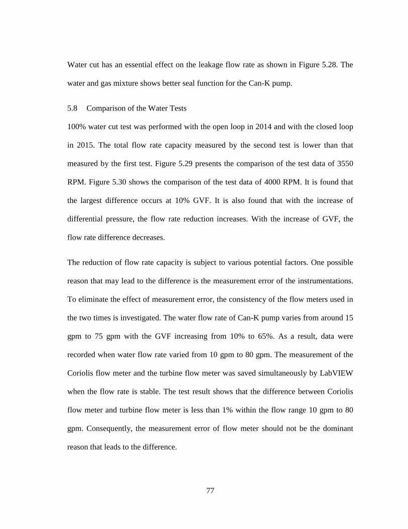
77
Water cut has an essential effect on the leakage flow rate as shown in Figure 5.28. The
water and gas mixture shows better seal function for the Can-K pump.
5.8 Comparison of the Water Tests
100% water cut test was performed with the open loop in 2014 and with the closed loop
in 2015. The total flow rate capacity measured by the second test is lower than that
measured by the first test. Figure 5.29 presents the comparison of the test data of 3550
RPM. Figure 5.30 shows the comparison of the test data of 4000 RPM. It is found that
the largest difference occurs at 10% GVF. It is also found that with the increase of
differential pressure, the flow rate reduction increases. With the increase of GVF, the
flow rate difference decreases.
The reduction of flow rate capacity is subject to various potential factors. One possible
reason that may lead to the difference is the measurement error of the instrumentations.
To eliminate the effect of measurement error, the consistency of the flow meters used in
the two times is investigated. The water flow rate of Can-K pump varies from around 15
gpm to 75 gpm with the GVF increasing from 10% to 65%. As a result, data were
recorded when water flow rate varied from 10 gpm to 80 gpm. The measurement of the
Coriolis flow meter and the turbine flow meter was saved simultaneously by LabVIEW
when the flow rate is stable. The test result shows that the difference between Coriolis
flow meter and turbine flow meter is less than 1% within the flow range 10 gpm to 80
gpm. Consequently, the measurement error of flow meter should not be the dominant
reason that leads to the difference.
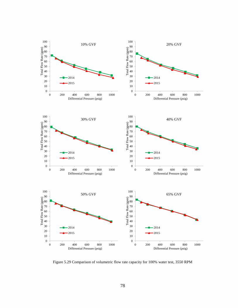
78
Figure 5.29 Comparison of volumetric flow rate capacity for 100% water test, 3550 RPM
0
10
20
30
40
50
60
70
80
90
100
0 200 400 600 800 1000
Tota
l F
low
Rat
e (g
pm
)
Differential Pressure (psig)
10% GVF
2014
2015
0
10
20
30
40
50
60
70
80
90
100
0 200 400 600 800 1000
Tota
l F
low
Rat
e (g
pm
)
Differential Pressure (psig)
20% GVF
2014
2015
0
10
20
30
40
50
60
70
80
90
100
0 200 400 600 800 1000
Tota
l F
low
Rat
e (g
pm
)
Differential Pressure (psig)
30% GVF
2014
2015
0
10
20
30
40
50
60
70
80
90
100
0 200 400 600 800 1000
Tota
l F
low
Rat
e (g
pm
)
Differential Pressure (psig)
40% GVF
2014
2015
0
10
20
30
40
50
60
70
80
90
100
0 200 400 600 800 1000
Tota
l F
low
Rat
e (g
pm
)
Differential Pressure (psig)
50% GVF
2014
2015
0
10
20
30
40
50
60
70
80
90
100
0 200 400 600 800 1000
Tota
l F
low
Rat
e (g
pm
)
Differential Pressure (psig)
65% GVF
2014
2015

79
Figure 5.30 Comparison of volumetric flow rate capacity for 100% water test, 4000 RPM
0
10
20
30
40
50
60
70
80
90
100
0 200 400 600 800 1000
Tota
l F
low
Rat
e (g
pm
)
Differential Pressure (psig)
10% GVF
2014
2015
0
10
20
30
40
50
60
70
80
90
100
0 200 400 600 800 1000
Tota
l F
low
Rat
e (g
pm
)
Differential Pressure (psig)
20% GVF
2014
2015
0
10
20
30
40
50
60
70
80
90
100
0 200 400 600 800 1000
Tota
l F
low
Rat
e (g
pm
)
Differential Pressure (psig)
30% GVF
2014
2015
0
10
20
30
40
50
60
70
80
90
100
0 200 400 600 800 1000
Tota
l F
low
Rat
e (g
pm
)
Differential Pressure (psig)
40% GVF
2014
2015
0
10
20
30
40
50
60
70
80
90
100
0 200 400 600 800 1000
Tota
l F
low
Rat
e (g
pm
)
Differential Pressure (psig)
50% GVF
2014
2015
0
10
20
30
40
50
60
70
80
90
100
0 200 400 600 800 1000
Tota
l F
low
Rat
e (g
pm
)
Differential Pressure (psig)
65% GVF
2014
2015

80
Figure 5.31 Effect of temperature on volumetric flow capacity
The flow rate capacity is also significantly affected by the inlet pressure and the outlet
pressure. As a result, pressure transducers were recalibrated. It is found that
measurement error of the pressure transducer at the pump inlet is less than 0.6 psig, and
the error at the pump outlet is less than 5 psig. From the curve of flow rate capacity, it
can be conclude that the error of the pressure transducer can’t be the dominant reason of
the difference.
The temperature may also be a potential effect on the pump performance. To confirm the
effect of temperature, the pump was operated with different inlet temperatures at 3550
RPM, 10% GVF and 600 psig differential pressure. As shown in Figure 5.31, the
temperature has little effect on the flow rate capacity.
38
39
40
41
42
43
44
75 85 95 105 115
To
tal
Flo
w R
ate
(gp
m)
Temperature (°F)
10% GVF

81
Instruments have been demonstrated to work well. Thus, it is necessary to investigate the
pump itself. Since the change of certain parameter of pump can have an important effect
on the pump performance. As a result, it is highly possible that there is something
different in the pump between the two tests. However, there is no way to have an
internal investigation of the dimensions of the Can-K pump in the lab. This is can only
feasible when it ships back to the manufactory.
5.9 Performance Comparison of Colfax Pump and Can-K Pump
Patil [23] investigated the multiphase performance of a MR-200 Colfax twin screw
pump. Experimental tests were performed with GVF ranging from 50% to 100% at
different differential pressures. The pump was operated with various speeds and suction
pressures. In this section, steady state performance was analyzed for the two twin screw
pumps with different design. Since the Colfax pump was only tested with water, only the
100% water cut test data of Can-K pump is selected in the following analysis.
5.9.1 Volumetric Flow Rate Capacity
Since the Colfax pump is a double-end pump, its flow rate capacity drops dramatically
when differential pressure increases to 250 psig. The Maximum working pressure of the
Colfax pump is rated 490 psig. However, the Can-K pump can work with differential
pressure up to 1000 psig. The Can-K pump owns much more seals than the Colfax
pump, which enable it to maintain the performance at extreme high differential pressure.
The Colfax owns a larger flow rate capacity due to its larger sizes. The theoretical flow

82
rate capacity of the Colfax pump is 651 gpm at 1800 RPM, while the theoretical flow
rate capacity of the Can-K pump is 113.5 gpm at 4000 RPM.
5.9.2 Leakage Flow Rate
The Colfax pump has a larger volumetric flow rate capacity while the flow rate capacity
of Can-K pump is relatively smaller since the size of Can-K pump has to be designed to
fit in the oil well. As a result, the double-end pump is generally used as a surface
multiphase pump, while the Can-K pump can be used as a subsurface pump.
The leakage flow of Colfax pump shows the same pattern with that of Can-K pump. For
the single phase test, the leakage flow increases with the increase of pump speed. For the
two phase test with the GVF above 50%, the leakage flow decreases with the increase of
pump speed. However, it is found that the leakage flow rate of Colfax pump is more
subject to pump speed, especially at high differential pressure. As shown in Figure 5.32,
the leakage flow rate increases rapidly as the pump speed increases.

83
Figure 5.32 Effect of speed on leakage flow for different GVF at 100 psig inlet pressure, Colfax pump
0
50
100
150
200
250
0 50 100 150 200 250
Lea
kag
e F
low
(gp
m)
Differential Pressure (psig)
50% GVF
900 RPM
1350 RPM
1800 RPM
0
50
100
150
200
250
0 50 100 150 200 250
Lea
kag
e F
low
(gp
m)
Differential Pressure (psig)
70% GVF
900 RPM
1350 RPM
1800 RPM
0
50
100
150
200
250
0 50 100 150 200 250
Lea
kag
e F
low
(gp
m)
Differential Pressure (psig)
90% GVF
900 RPM
1350 RPM
1800 RPM
0
50
100
150
200
250
0 50 100 150 200 250
Lea
kag
e F
low
(gp
m)
Differential Pressure (psig)
95% GVF
900 RPM
1350 RPM
1800 RPM
0
50
100
150
200
250
0 50 100 150 200 250
Lea
kag
e F
low
(gp
m)
Differential Pressure (psig)
98% GVF
900 RPM
1350 RPM
1800 RPM
0
50
100
150
200
250
0 50 100 150 200 250
Lea
kag
e F
low
(gp
m)
Differential Pressure (psig)
100% GVF
900 RPM
1350 RPM
1800 RPM

84
5.9.3 Volumetric Efficiency
Figure 5.33 shows the comparison of volumetric efficiency. Volumetric efficiency of
Colfax pump is consistently higher than that of Can-K pump. Note that the pump speed
of Colfax pump is less than that of Can-K pump. It can be expected that the volumetric
efficiency of Colfax pump is even higher than the Can-K pump if they can be operated at
the same speed. Information of the clearance size is not available for the Can-K pump.
The size of circumferential clearance of Can-K pump can be estimated with the
analytical model of Vetter. It is found that the circumferential clearance of Can-K pump
is around 0.5 mm, which is much larger than that of Colfax pump. However, the rotor
diameter and the displacement per revolution of Colfax pump are much larger than that
of Can-K pump. Thus, the leakage of Colfax pump may has less effect on the volumetric
efficiency.

85
Figure 5.33 Volumetric efficiency of Colfax pump at 100 psig inlet pressure, 1800 RPM
Figure 5.34 Volumetric efficiency for Colfax pump at 100 psig inlet pressure, 1800 RPM
0.6
0.65
0.7
0.75
0.8
0.85
0.9
0.95
1
0 50 100 150 200 250 300
Vo
lum
etri
c E
ffic
iency
Differential Pressure (psig)
Colfax Pump
50% GVF
70% GVF
90% GVF
95% GVF
98% GVF
99% GVF
100% GVF
0.6
0.7
0.8
0.9
1
50 60 70 80 90 100
Vo
lum
etri
c E
ffic
iency
GVF (%)
Colfax Pump
dP = 50 psi
dP = 100 psi
dP = 150 psi
dP = 200 psi
dP = 250 psi

86
Figure 5.35 Volumetric efficiency for Can-K pump at 100 psig inlet pressure, 4000 RPM
As shown in Figure 5.34, the volumetric efficiency of Colfax pump maximizes around
95% GVF. The Colfax pump has a liquid recirculation system which is used to inject a
specific amount of liquid into the pump to seal the clearance at extremely high GVF
operation. As a result, the Colfax pump can be operated with extremely high GVF flows.
Note that the GVF for Colfax pump is skid based data, which is calculated by the
following equation,
𝐺𝑉𝐹 =
𝑄𝑔
𝑄𝑙 + 𝑄𝑔 5.3
0.2
0.3
0.4
0.5
0.6
0.7
0.8
0.9
1
10 30 50 70 90
Vo
lum
etri
c E
ffic
iency
GVF (%)
Can-K Pump
dP = 100 psi
dP = 200 psi
dP = 400 psi
dP = 600 psi
dP = 800 psi
dP = 1000 psi

87
As a result, this GVF doesn’t reflect the real GVF at the entrance of the Colfax pump,
since the skid based GVF doesn’t include the effect of the recirculation. The real GVF is
also referred to as pump based GVF, which can be calculated by the following equation,
𝐺𝑉𝐹 =
𝑄𝑔
𝑄𝑙 + 𝑄𝑔 + 𝑄𝑟 5.4
In this section, the GVF of Colfax pump is skid based data. The skid based GVF is
generally larger than the real GVF as shown in Figure 5.36, since it doesn’t include the
recirculation flow.
Figure 5.36 Comparison of skid based GVF and pump based GVF
40
50
60
70
80
90
100
50 100 150 200 250 300
Pum
p B
ased
GV
F (
%)
Differential Pressure (psig)
50% GVF
70% GVF
90% GVF
95% GVF
100% GVF

88
For the Can-K pump, the volumetric efficiency always increases with the increase of
GVF. However, since there is no recirculation system for the Can-K pump, it was only
tested to 85% GVF. But it can be expected that the volumetric efficiency will begin to
decrease with the increase of GVF above this GVF.
5.9.4 Mechanical Efficiency
Figure 5.37 shows the comparison of the mechanical efficiency. It is found that the
mechanical efficiency of Colfax pump is much higher than the Can-K pump. As shown
in Figure 5.37, the mechanical efficiency of the Colfax pump is generally higher than 50%
within the test conditions. However, mechanical efficiency of Can-K pump is less than
30%. Since the Can-K pump is a multistage pump, there are many more seals in the Can-
K pump. The design of the Can-K pump results in more internal friction losses.
As shown in Figure 5.37, the mechanical efficiency of Colfax pump is more dependent
upon GVF. With the 200 psig differential pressure, the mechanical efficiency at 50%
GVF is about 58%, while it is only 25.6% at 100% GVF. However, the GVF has little
effect on the Can-K pump. Additionally, the maximum mechanical efficiency for the
Colfax pump occurs at about 150 psig differential pressure, while the maximum
mechanical efficiency for the Colfax pump occurs at about 600 psig.

89
Figure 5.37 Comparison of mechanical efficiency
0
0.1
0.2
0.3
0.4
0.5
0.6
0.7
0.8
0 200 400 600 800 1000
Mec
han
ical
Eff
icie
ncy
Differential Pressure (psig)
Comparison of Mechanical EfficiencyColfax 50% GVF
Colfax 70% GVF
Colfax 90% GVF
Colfax 100% GVF
Can-K 10% GVF
Can-K 50% GVF
Can-K 65% GVF
Can-K 85% GVF

90
6 MULTIPHASE TWIN-SCREW PUMP MODEL
This chapter represents the development of an analytical model to predict the multiphase
performance of the twin screw pumps. As mentioned in the literature review, previous
research of the analytical model is still insufficient to reflect the flowing condition in the
twin screw pump. Most of the previous models didn’t consider the compressibility of the
leakage flow. Besides, none of the previous models try to predict the performance of the
multistage pump. Hence, a new model is necessary to be created to model the leakage
flow in the twin screw pump.
In this model, the compressibility of leakage flow will be investigated. It is assumed that
the gas mass fraction is uniform at an arbitrary position in the chambers and clearances
at the low GVFs. At the high GVFs the gas mass fraction in the clearance is smaller than
the gas mass fraction in the chamber due to centrifugal force. In this model, the gas mass
fraction in the clearance is assumed to be 80% of the gas mass fraction in the chamber.
The leakage flow is considered as compressible flow in the clearances. The choked flow
condition may have an essential effect on the leakage flow rate. In this research, the
possibility of the choked flow condition at the exit of clearance will be investigated.
Previous models are mainly applied on the single-stage pump. In this research, a new
model is proposed to predict the multiphase performance of a multi-stage twin screw
pump. The pressure distribution along the stages is modeled by an empirical equation.

91
6.1 Simplification of Twin Screw Pump Working Process
The working process of a real twin screw pump is too complex to analyze by an
analytical method. It is necessary to make requisite simplifications and assumptions
before the simulation. In this model, the twin screw pump is simplified to a series of the
chambers divided by discs which moving axially from the suction side to the discharge
side. The fluids enter and exit the chambers through the clearances. It is assumed that the
liquid and the gas are fully mixed at an arbitrary point in the pump.
Direction of conveyance
Direction of leakage
,out outp T,in inp T
1 2 3
Figure 6.1 Simplification of the twin screw pump
The model is established with the assumptions and simplifications below:
• The gas is considered as ideal gas
• The leakage flow is assumed as two phase compressible flow
• The circumferential leakage accounts for 80% of the total leakage
• Division of one revolution into small time segments
92
• Chamber pressure and temperature remain constant in one time segment
• Leakage flow is one-dimensional compressible flow; flow in the circumferential
direction is neglected
• At the end of one rotation, the 𝑖𝑡ℎ chamber become the 𝑖 + 1𝑡ℎ chamber; the last
chamber vanished; a new chamber is created at the pump inlet
During the operation, the closed chambers move continuously from the suction side to
the discharge side. The pressure and temperature keep changing all the time as well.
Hence, the period of one revolution is divided into multiple time steps in this model.
And the distance the chamber moved forward in one revolution is also divided into
appropriate distance. During one time step, the discs remain stationary. The pressure and
the temperature in the chambers are assumed to be constant. At the next time step, the
discs jump to the next corresponding positions. Thus, the working process is largely
simplified. It is only necessary to find the conditions during the time steps. Since the
pressure and temperature in the chamber remain constant during one time step, the
leakage flow rate can be calculated by an analytical method.
6.2 Geometric Parameters
With these simplifications and assumptions, an analytical model can be proposed to
present the working process of twin screw pump. However, to start the simulation, the
following geometric parameters of pump is requisite to import into the computer
program,
• Screw outer diameter
• Screw root diameter

93
• Screw pitch
• Screw length
• Thickness of the screw threads
• Displacement per revolution
• Size of circumferential clearance
Typically the geometric parameters are provided by the manufacturer. However,
sometimes the actual size of circumferential clearance is not available or the
manufacturer doesn’t want to disclose the information. In this circumstance, the size of
the circumferential clearance can be estimated based upon pure water experimental
performance data. Assuming the leakage area can be represented with a hydraulic
diameter, so the Bernoulli’s Equation for a pipe flow can be used.
𝑝𝑖𝑛
𝜌𝑙+
1
2𝑣𝑖𝑛
2 −𝑝𝑜𝑢𝑡
𝜌𝑙−
1
2 𝑣𝑜𝑢𝑡
2 =1
2𝑓
𝑙
𝑑ℎ𝑣𝑖𝑛
2 6.1
Since for pure liquid flow 𝑉𝑖𝑛2 = 𝑉𝑜𝑢𝑡
2 . Thus,
∆𝑝 =1
2𝑓
𝑙
𝑑ℎ𝜌𝑙𝑣𝑖𝑛
2 6.2
Since 𝑑ℎ = 2𝑐 , the size of circumferential clearance can be solved by the following
equation,
𝑐 =𝑓𝐿𝜌𝑙𝑣𝑖𝑛
2
4∆𝑝 6.3
For the laminar flow,
94
𝑓 =96
𝑅𝑒 6.4
For the turbulent smooth clearance,
𝑓 =0.316
𝑅𝑒0.25 6.5
In this research, the sizes of circumferential clearance for Can-K pump and Colfax pump
are estimated.
6.3 Leakage Flow in the Clearance
To predict the behavior of twin screw pump, it is important to model the leakage flow in
the clearance. As shown in Figure 6.2, the circumferential clearance connects two
adjacent chambers. In this model, the chamber is regarded as a reservoir where the fluid
is static. When the fluid is injected into the clearance due to differential pressure
between two adjacent chambers, the fluid will be accelerated from static at the entrance
as shown in Figure 6.3. If the pressure at the clearance entrance is known, the clearance
inlet GVF, density and velocity can be solved with equation 6.6 - 6.8 by Brennen [26].
𝛼 =𝑝0𝛼0(1 − 𝛼)
𝑝 + 𝛼0(𝑝0 − 𝑝) 6.6
𝜌 =
1 − 𝛼
1 − 𝛼0∙ 𝜌0
6.7
𝑢2 =
2𝑝0𝛼0
𝜌0[1 − 𝛼0
𝛼0−
1 − 𝛼
𝛼+ 𝐼𝑛 (
(1 − 𝛼0)𝛼
𝛼0(1 − 𝛼))]
6.8

95
Figure 6.2 Leakage flow in the circumferential clearance
Figure 6.3 Fluids acceleration in the entrance of clearance
However, the pressure at the clearance entrance is typically unknown in the beginning of
calculation. Instead, only the pressure and temperature in the upstream and downstream
chambers are known. Hence, the inlet velocity must be found by iteration. To start
calculation, an initial inlet pressure is assumed at the beginning of calculation. Then the

96
flow conditions in the clearance can be calculated with a Fanno flow model. The inlet
pressure is adjusted according to the condition at the exit of clearance until the exit
pressure equals to the downstream chamber pressure or the leakage flow is choked at the
exit. Figure 6.4 shows the computer algorithm to calculate the leakage flow.
Figure 6.4 Computer program algorithm

97
The flow in the clearance is solved using a two phase Fanno flow model. Since the size
of the clearance is much smaller than the length of the clearance and the perimeter of the
screw, the leakage flow through the circumferential clearances can be simplified to a
one-dimensional adiabatic flow in a duct, which can also be referred to as Fanno flow.
With knowing the inlet conditions, the downstream conditions can be calculated with the
following differential equations. The change of Mach number is related with a small
distance by the following differential equation,
𝑓
𝐷ℎ𝑑𝑥 = 2
(1 − 𝑀2)
(1 +𝑘 − 1
2 𝑀2) ∙ 𝑘𝑀2
𝑑𝑀
𝑀 6.9
Control Volume
T
p
M
v
T+dT
p+dp
M+dM
v+dv
dx
Figure 6.5 Control volume of fanno flow in the duct
With the local Mach number, the change of the pressure and temperature can be
calculated with the following equations,

98
𝑑𝑇
𝑇= −
(𝑘 − 1)𝑀𝑑𝑀
1 +𝑘 − 1
2 𝑀2 6.10
𝑑𝑃
𝑃= −
𝑑𝑀
𝑀+ 0.5
𝑑𝑇
𝑇
6.11
For the two phase flow, the fluid properties are different from single component flow. In
this model, the density and the viscosity of the mixture are the weighted averages of
liquid and gas.
𝜌𝑚 = 𝛼𝜌𝑔 + (1 − 𝛼)𝜌𝑙 6.12
𝜇𝑚 = 𝛼𝜇𝑔 + (1 − 𝛼)𝜇𝑙 6.13
The friction factor is calculated according to local Re number. For the laminar flow,
𝑓 =96
𝑅𝑒 6.14
For the turbulent smooth clearance,
𝑓 =0.316
𝑅𝑒0.25 6.15
Due to the intensive mixing process in the pump, the heat and momentum transfer
process is so rapid that the leakage flow can be treated as homogenous flow. The
velocity and the temperature of the two phases are considered to be the same.
𝑅𝑒 =𝜌𝑣𝐷
𝜇 6.16
Where 𝑣 = 𝑀𝑐, and 𝑐 is the speed of sound in the mixture. The viscosity of gas can be
obtained through the Sutherland’s formula,

99
𝜇 = 𝜇0
𝑎
𝑏(
𝑇
𝑇0)
1.5
6.17
Where 𝑎, 𝑏, 𝜇0 and 𝑇0 are constants.
Until now, the leakage flow has been modeled during one time step. Therefore, the mass
balance in the chamber can be calculated with the leakage flow rate. The change of
pressure and temperature in the chamber can also be found with energy conservation.
6.4 Sonic Speed of Homogeneous Two Phase Flow
In a constant area duct, the speed of compressible flow can’t exceed the local speed of
sound. As a result, the maximum Mach number is 1 at the exit of the clearance. In this
case, the leakage flow velocity will not increase even with lower downstream pressure.
In this circumstance, the leakage flow velocity is largely affected by the sonic speed of
the two phase flow. As a result, it is necessary to discuss the characteristics of the sonic
speed of homogeneous two phase flow. Sonic speed of homogeneous two phase flow
represents distinguished property compared with single phase flow. The sonic speed of a
two phase liquid/gas flow can be expressed with the following equation, [26]
1
𝑐2= [𝜌𝑙(1 − 𝛼) + 𝜌𝑔𝛼] [
𝛼
𝑘𝑝+
(1 − 𝛼)
𝜌𝑙𝑐𝑙2 ] 6.18
In many applications, 𝛼
𝑘𝑝≫
(1−𝛼)
𝜌𝑙𝑐𝑙2 thus equation 6.3 can be simplified to, [26]
1
𝑐2=
𝛼
𝑘𝑝∙ [𝜌𝑙(1 − 𝛼) + 𝜌𝑔𝛼] 6.19

100
Figure 6.6 shows the variation of sonic speed for the two phase water/air flow with
different GVF at 100 psig. It is found that the sonic speed of homogenous two phase
flow becomes the minimum with GVF around 60%. The sonic speed at 60% GVF is
about 68 m/s, which is much lower that of pure water or pure air.
Figure 6.6 Sonic speed of two phase water/air flow at 100 psig
6.5 Mass Balance in the Chambers
According to Vetter, the circumferential gap flow contributes 80% percent of the total
leakage, 15% of the total leakage is through the radial clearance, and another 5% is due
to the flank leakage. As a result, the prediction of the circumferential gap flow is
0
200
400
600
800
1000
0 20 40 60 80 100
So
nic
Sp
eed
(m
/s)
GVF (%)
sonic speed

101
dominant to determine the accuracy of the new leakage model. In this model, only
circumferential leakage flow is calculated in the computer program. The radial leakage
and the flank leakage are assumed to be 15% and 5% of total leakage separately.
,in g,in,lm m
Figure 6.7 Mass balance in one closed chamber
Figure 6.7 shows the liquid and the gas flow in and out of a chamber from the
circumferential clearance. The mass balance for the chamber can be calculated by the
following differential equations,
𝑑𝑚𝑙,𝑖
𝑑𝑡=
𝑑𝑚𝑙,𝑖𝑛
𝑑𝑡−
𝑑𝑚𝑙,𝑜𝑢𝑡
𝑑𝑡 6.20
𝑑𝑚𝑔,𝑖
𝑑𝑡=
𝑑𝑚𝑔,𝑖𝑛
𝑑𝑡−
𝑑𝑚𝑔,𝑜𝑢𝑡
𝑑𝑡 6.21
The rapid rotating of rotors leads to intensive mixing between the liquid and the gas.
Therefore, the pressure and the temperature can be considered to be uniform in the
chamber. The liquid and the gas is assumed to be fully mixed. As a result, it is assumed
that the flow in the clearance is homogenous.
102
It is assumed that the chamber is adiabatic. According to the energy balance equation,
𝑑𝑈𝑖
𝑑𝑡= (
𝑑𝑚𝑙,𝑖𝑛
𝑑𝑡∙ ℎ𝑙,𝑖𝑛 +
𝑑𝑚𝑔,𝑖𝑛
𝑑𝑡∙ ℎ𝑔,𝑖𝑛) − (
𝑑𝑚𝑙,𝑜𝑢𝑡
𝑑𝑡∙ ℎ𝑙,𝑜𝑢𝑡 +
𝑑𝑚𝑔,𝑜𝑢𝑡
𝑑𝑡∙ ℎ𝑔,𝑜𝑢𝑡)
6.22
With knowing the condition of the entering and leaving leakages, the temperature in the
next time step can be calculated.
Therefore, the chamber pressure in the next time step can be calculated by the following
equation,
𝑝𝑖, 𝑡+∆𝑡 = 𝜌𝑅𝑇𝑖, 𝑡+∆𝑡 6.23
6.6 Solution Methodology
The computer algorithm is shown in Figure 6.8. To start the simulation, an arbitrary
initial pressure and temperature distribution need to be entered into the computer
program. With the initial pressure and temperature distribution, the leakage flow rate can
be calculated within one time step. Then the mass and pressure distribution in the
chamber will be modified according to leakage flow rate, which will be used as initial
condition in the calculation of the next time step.

103
1
,0 1,
1
,0 1,
1
,0 1,
1
, 2, , 1
, 2, , 1
, 2, , 1
N N
i i
N N
i i
N N
i i
N N
i p
T i
m
p
i
P
m p
P
T
t t t
0t
?t
1
, , ?N N
i imm
i i
leak leak
Calculate the leakage
flow rate m and V
No
Yes
No
Yes
1
, ,m mN N i i
i t i t leak leakt m m
, , N N
i t i tCalculate P and T
i,0 i,0 i,0, , ;
1;
N N NP T m
N
1
,
0
1
i
leak leak t
t
leakvo l
cham
V t V
V
V
Figure 6.8 Computer program algorithm

104
After one revolution, the 𝑖𝑡ℎ chamber will be the 𝑖 + 1𝑡ℎ chamber, the chamber
condition at the end of last revolution are set to be the initial condition for the calculation
of next revolution.
𝑝1,0𝑁+1 = 𝑝𝑖𝑛, 𝑝𝑖,0
𝑁+1 = 𝑝𝑖−1,𝜏𝑁 6.24
𝑇1,0𝑁+1 = 𝑇𝑖𝑛, 𝑇𝑖,0
𝑁+1 = 𝑇𝑖−1,𝜏𝑁 6.25
The pump is considered to be steady state when the flow rate of one revolution is equal
to that of last revolution. In this case, the program will stop and predictions of steady
state condition will be saved.
6.7 Modeling of Multistage Twin Screw Pump
Multistage twin screw pump consists of more than one stage, and each stage can be
considered as a single stage pump. The model isn’t able to be applied directly on the
multistage twin screw pump. Since only the pressure and temperature at the pump inlet
and the outlet is known, it is necessary to find the pressure and temperature distribution
along the stages. Based on the experimental data, the following empirical equation of
pressure distribution has be developed,
𝑝𝑖 − 𝑝𝑖𝑛
𝑝𝑜𝑢𝑡 − 𝑝𝑖𝑛= (
𝑖
𝑁)
2𝛼
6.26
The temperature is assumed to be linearly distributed along the stages. To prove the
validation of an analytical model, it is necessary to make comparisons between the
predicted and experimental results. In the next chapter, experimental data will be
selected to verify the prediction of this model.

105
7 MULTIPHASE TWIN-SCREW PUMP MODEL VALIDATION
To verify the validation of this model, the model will be used to predict the behavior of
twin screw pumps in this chapter. The predictions of volumetric efficiency will be
compared with experiment data to determine the model’s accuracy. The validation
procedure utilizes experimental data for the following pumps:
• Leistritz L4MG Twin Screw Pump
• Colfax MR-200 Multiphase Twin Screw Pump
• Flowserve MP1 Twin Screw Pump
• Can-K 425 ESTSP
In addition, the pressure distribution and flow status in the pump will be presented. The
choked condition and its effect on the pump performance will also be investigated.
7.1 Prediction of Pressure Distribution in the Twin Screw Pump
Pressure distribution in the twin screw pump of two phase flow represents unique
characteristics compared with the pressure distribution of single phase flow. Typically,
the pressure is linearly distributed along the pump screws from the suction side to
discharge side for the single phase flow. However, the shape of the pressure distribution
changes from linear to concave up when the pump is operated with two phase flow.
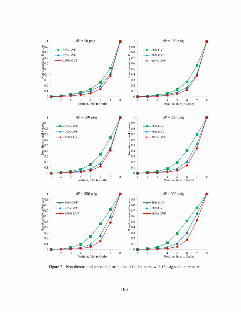
106
Figure 7.1 Non-dimensional pressure distribution of Colfax pump with 15 psig suction pressure
0
0.1
0.2
0.3
0.4
0.5
0.6
0.7
0.8
0.9
1
1 2 3 4 5 6 7 8
Non
-dim
ensi
on
al P
ress
ure
Position, Inlet to Outlet
dP = 50 psig
50% GVF
70% GVF
100% GVF
0
0.1
0.2
0.3
0.4
0.5
0.6
0.7
0.8
0.9
1
1 2 3 4 5 6 7 8
Non
-dim
ensi
on
al P
ress
ure
Position, Inlet to Outlet
dP = 100 psig
50% GVF
70% GVF
100% GVF
0
0.1
0.2
0.3
0.4
0.5
0.6
0.7
0.8
0.9
1
1 2 3 4 5 6 7 8
Non
-dim
ensi
on
al P
ress
ure
Position, Inlet to Outlet
dP = 150 psig
50% GVF
70% GVF
100% GVF
0
0.1
0.2
0.3
0.4
0.5
0.6
0.7
0.8
0.9
1
1 2 3 4 5 6 7 8
Non
-dim
ensi
on
al P
ress
ure
Position, Inlet to Outlet
dP = 200 psig
50% GVF
70% GVF
100% GVF
0
0.1
0.2
0.3
0.4
0.5
0.6
0.7
0.8
0.9
1
1 2 3 4 5 6 7 8
Non
-dim
ensi
on
al P
ress
ure
Position, Inlet to Outlet
dP = 250 psig
50% GVF
70% GVF
100% GVF
0
0.1
0.2
0.3
0.4
0.5
0.6
0.7
0.8
0.9
1
1 2 3 4 5 6 7 8
Non
-dim
ensi
on
al P
ress
ure
Position, Inlet to Outlet
dP = 300 psig
50% GVF
70% GVF
100% GVF

107
Figure 7.2 Non-dimensional pressure distribution of Colfax pump with 100 psig suction pressure
0
0.1
0.2
0.3
0.4
0.5
0.6
0.7
0.8
0.9
1
1 2 3 4 5 6 7 8
Non
-dim
ensi
on
al P
ress
ure
Position, Inlet to Outlet
dP = 50 psig
50% GVF
70% GVF
100% GVF
0
0.1
0.2
0.3
0.4
0.5
0.6
0.7
0.8
0.9
1
1 2 3 4 5 6 7 8
Non
-dim
ensi
on
al P
ress
ure
Position, Inlet to Outlet
dP = 100 psig
50% GVF
70% GVF
100% GVF
0
0.1
0.2
0.3
0.4
0.5
0.6
0.7
0.8
0.9
1
1 2 3 4 5 6 7 8
Non
-dim
ensi
on
al P
ress
ure
Position, Inlet to Outlet
dP = 150 psig
50% GVF
70% GVF
100% GVF
0
0.1
0.2
0.3
0.4
0.5
0.6
0.7
0.8
0.9
1
1 2 3 4 5 6 7 8
Non
-dim
ensi
on
al P
ress
ure
Position, Inlet to Outlet
dP = 200 psig
50% GVF
70% GVF
100% GVF
0
0.1
0.2
0.3
0.4
0.5
0.6
0.7
0.8
0.9
1
1 2 3 4 5 6 7 8
Non
-dim
ensi
on
al P
ress
ure
Position, Inlet to Outlet
dP = 250 psig
50% GVF
70% GVF
100% GVF
0
0.1
0.2
0.3
0.4
0.5
0.6
0.7
0.8
0.9
1
1 2 3 4 5 6 7 8
Non
-dim
ensi
on
al P
ress
ure
Position, Inlet to Outlet
dP = 300 psig
50% GVF
70% GVF

108
Steady state pressure distribution of the Colfax pump are presented by Figure 7.1 and
Figure 7.2. Obviously GVF has a significant influence on the pressure distribution. With
the increase of GVF, the pressure rise becomes steeper near the discharge side.
7.2 Volumetric Efficiency Prediction of Colfax Pump
The Colfax pump was tested by Patil [23] with two phase flow. Water and air were
selected as testing fluids. The pump was tested with different suction pressure, GVF, and
differential pressure. Steady state and transient pump performance were investigated. In
this section, the experimental data of steady state is selected to compare with simulation
results. The comparison of simulation and experimental results is shown in the Figure
7.3 and Figure 7.4. The simulation results show the same trends as the experimental data
within the test conditions.
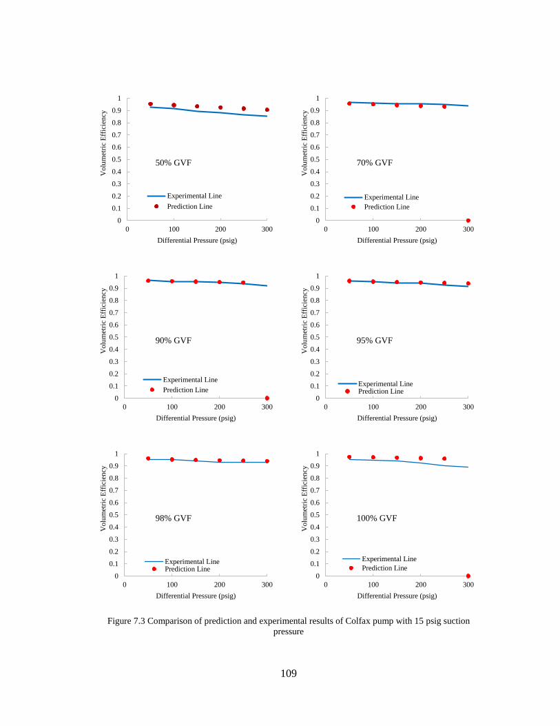
109
Figure 7.3 Comparison of prediction and experimental results of Colfax pump with 15 psig suction
pressure
0
0.1
0.2
0.3
0.4
0.5
0.6
0.7
0.8
0.9
1
0 100 200 300
Volu
met
ric
Eff
icie
ncy
Differential Pressure (psig)
50% GVF
Experimental Line
Prediction Line
0
0.1
0.2
0.3
0.4
0.5
0.6
0.7
0.8
0.9
1
0 100 200 300
Volu
met
ric
Eff
icie
ncy
Differential Pressure (psig)
70% GVF
Experimental Line
Prediction Line
0
0.1
0.2
0.3
0.4
0.5
0.6
0.7
0.8
0.9
1
0 100 200 300
Volu
met
ric
Eff
icie
ncy
Differential Pressure (psig)
90% GVF
Experimental Line
Prediction Line
0
0.1
0.2
0.3
0.4
0.5
0.6
0.7
0.8
0.9
1
0 100 200 300
Volu
met
ric
Eff
icie
ncy
Differential Pressure (psig)
95% GVF
Experimental LinePrediction Line
0
0.1
0.2
0.3
0.4
0.5
0.6
0.7
0.8
0.9
1
0 100 200 300
Volu
met
ric
Eff
icie
ncy
Differential Pressure (psig)
98% GVF
Experimental LinePrediction Line
0
0.1
0.2
0.3
0.4
0.5
0.6
0.7
0.8
0.9
1
0 100 200 300
Volu
met
ric
Eff
icie
ncy
Differential Pressure (psig)
100% GVF
Experimental Line
Prediction Line
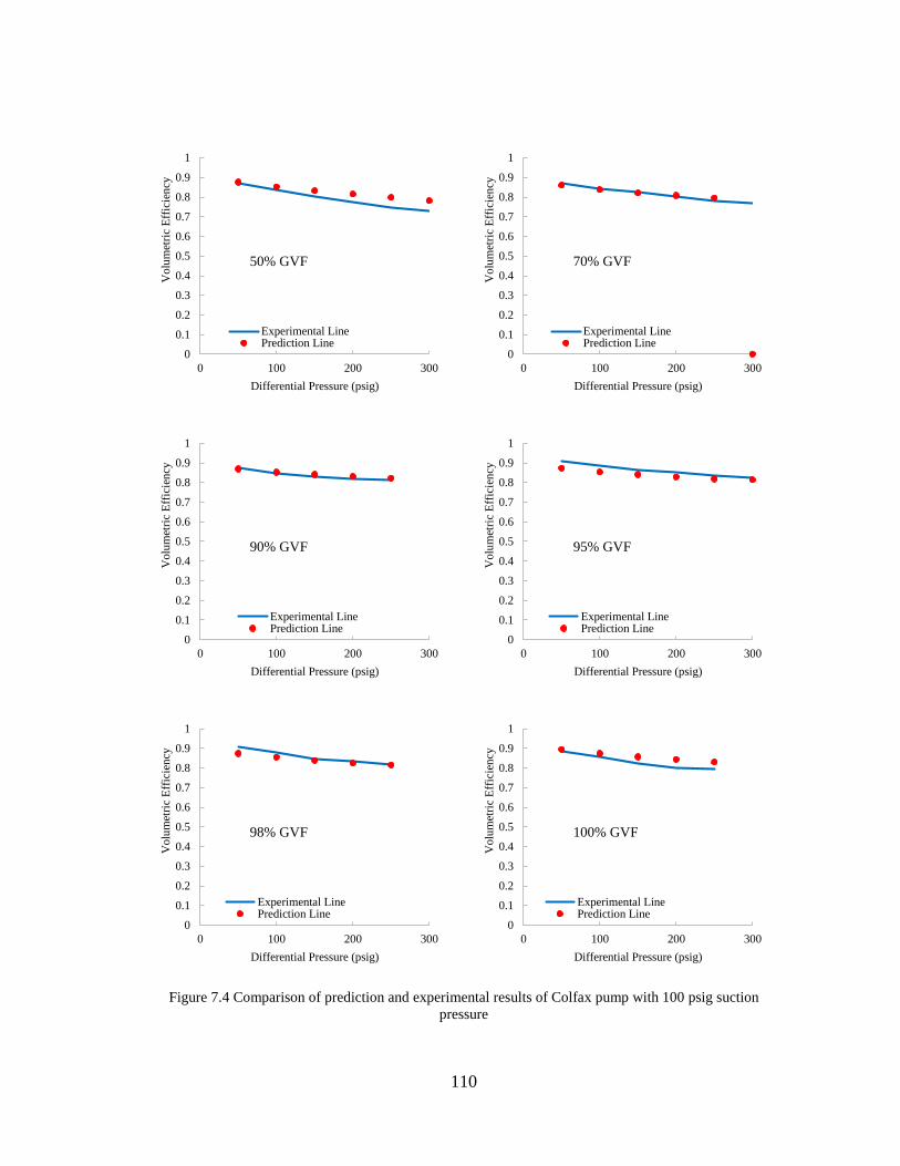
110
Figure 7.4 Comparison of prediction and experimental results of Colfax pump with 100 psig suction
pressure
0
0.1
0.2
0.3
0.4
0.5
0.6
0.7
0.8
0.9
1
0 100 200 300
Volu
met
ric
Eff
icie
ncy
Differential Pressure (psig)
50% GVF
Experimental LinePrediction Line
0
0.1
0.2
0.3
0.4
0.5
0.6
0.7
0.8
0.9
1
0 100 200 300
Volu
met
ric
Eff
icie
ncy
Differential Pressure (psig)
70% GVF
Experimental LinePrediction Line
0
0.1
0.2
0.3
0.4
0.5
0.6
0.7
0.8
0.9
1
0 100 200 300
Volu
met
ric
Eff
icie
ncy
Differential Pressure (psig)
90% GVF
Experimental LinePrediction Line
0
0.1
0.2
0.3
0.4
0.5
0.6
0.7
0.8
0.9
1
0 100 200 300
Volu
met
ric
Eff
icie
ncy
Differential Pressure (psig)
95% GVF
Experimental LinePrediction Line
0
0.1
0.2
0.3
0.4
0.5
0.6
0.7
0.8
0.9
1
0 100 200 300
Volu
met
ric
Eff
icie
ncy
Differential Pressure (psig)
98% GVF
Experimental LinePrediction Line
0
0.1
0.2
0.3
0.4
0.5
0.6
0.7
0.8
0.9
1
0 100 200 300
Volu
met
ric
Eff
icie
ncy
Differential Pressure (psig)
100% GVF
Experimental LinePrediction Line
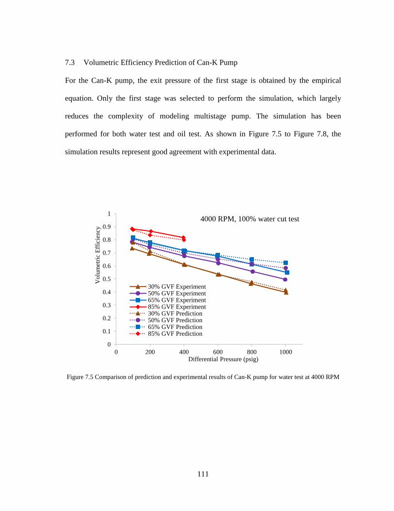
111
7.3 Volumetric Efficiency Prediction of Can-K Pump
For the Can-K pump, the exit pressure of the first stage is obtained by the empirical
equation. Only the first stage was selected to perform the simulation, which largely
reduces the complexity of modeling multistage pump. The simulation has been
performed for both water test and oil test. As shown in Figure 7.5 to Figure 7.8, the
simulation results represent good agreement with experimental data.
Figure 7.5 Comparison of prediction and experimental results of Can-K pump for water test at 4000 RPM
0
0.1
0.2
0.3
0.4
0.5
0.6
0.7
0.8
0.9
1
0 200 400 600 800 1000
Vo
lum
etri
c E
ffic
iency
Differential Pressure (psig)
4000 RPM, 100% water cut test
30% GVF Experiment50% GVF Experiment65% GVF Experiment85% GVF Experiment30% GVF Prediction50% GVF Prediction65% GVF Prediction85% GVF Prediction

112
Figure 7.6 Comparison of prediction and experimental results of Can-K pump for oil Test at 4000 RPM
Figure 7.7 Comparison of prediction and experimental results of Can-K pump for water test at 3550 RPM
0
0.1
0.2
0.3
0.4
0.5
0.6
0.7
0.8
0.9
1
0 200 400 600 800 1000
Vo
lum
etri
c E
ffic
iency
Differential Pressure (psig)
4000 RPM, 0% water cut test
30% GVF Experiment50% GVF Experiment70% GVF Experiment85% GVF Experiment30% GVF Prediction50% GVF Prediction70% GVF Prediction85% GVF Prediction
0
0.1
0.2
0.3
0.4
0.5
0.6
0.7
0.8
0.9
1
0 200 400 600 800 1000
Vo
lum
etri
c E
ffic
iency
Differential Pressure (psig)
3550 RPM, 100% water cut test
30% GVF Experiment
50% GVF Experiment
65% GVF Experiment
85% GVF Experiment
30% GVF Prediction
50% GVF Prediction
65% GVF Prediction
85% GVF Prediction

113
Figure 7.8 Comparison of prediction and experimental results of Can-K pump for oil test at 3550 RPM
7.4 Volumetric Efficiency Prediction of Leistritz Pump
The Leistritz pump was tested by Kroupa [21] with two phase flow. Water and air were
selected as testing fluids. Steady state pump performance was investigated with GVF
ranging from 50% to 100%. The effect of liquid recirculation loop was studied at high
GVFs. In this section, only the steady state performance data is selected to make the
comparison with simulation results. The comparison of prediction and experimental
results are shown in Figure 7.9. The prediction shows good agreement with experimental
results with GVF less than 90%. The prediction of volumetric efficiency is larger than
experimental data at 95% GVF and 100% GVF.
0
0.1
0.2
0.3
0.4
0.5
0.6
0.7
0.8
0.9
1
0 200 400 600 800 1000
Vo
lum
etri
c E
ffic
iency
Differential Pressure (psig)
3550 RPM, 0% water cut test
30% GVF Experiment
50% GVF Experiment
70% GVF Experiment
85% GVF Experiment
30% GVF Prediction
50% GVF Prediction
70% GVF Prediction
85% GVF Prediction

114
Figure 7.9 Comparison of prediction and experimental results of Leistritz pump
7.5 Volumetric Efficiency Prediction of Flowserve Pump
The Flowserve Pump was tested with oil and air. However, the experimental data of the
Flowserve pump is incomplete. The pump inlet pressure and testing temperature are
unavailable. The property of the working fluid is also unknown. In the simulation, the
inlet pressure is assumed to be 100 psig and the inlet temperature is assumed to be 80 °F.
Figure 7.6 shows the comparison between the prediction and experimental data. The
0
0.1
0.2
0.3
0.4
0.5
0.6
0.7
0.8
0.9
1
0 100 200 300
Volu
met
ric
Eff
icie
ncy
Differential Pressure (psig)
50% GVF
Experimental Line
Prediction Line
0
0.1
0.2
0.3
0.4
0.5
0.6
0.7
0.8
0.9
1
0 100 200 300
Volu
met
ric
Eff
icie
ncy
Differential Pressure (psig)
90% GVF
Experimental Line
Prediction Line
0
0.1
0.2
0.3
0.4
0.5
0.6
0.7
0.8
0.9
1
0 100 200 300
Volu
met
ric
Eff
icie
ncy
Differential Pressure (psig)
95% GVF
Experimental Line
Prediction Line
0
0.1
0.2
0.3
0.4
0.5
0.6
0.7
0.8
0.9
1
0 100 200 300
Volu
met
ric
Eff
icie
ncy
Differential Pressure (psig)
100% GVF
Experimental Line
Prediction Line

115
prediction shows the same trend with the experimental data. However, the test data
shows that the volumetric efficiency decreases rapidly when the differential pressure is
larger than 2000 psig. Since the relation of oil viscosity with temperature is not
available, the viscosity is set to be constant in the program. With the increase of
differential pressure, the viscosity will decrease due to increased temperature in the
pump. The decreased viscosity will reduce the friction resistance in the clearance, which
will lead to the increase of leakage flow rate.
Figure 7.10 Comparison of prediction and experimental results of Flowserve pump
0.2
0.3
0.4
0.5
0.6
0.7
0.8
0.9
1
0 500 1000 1500 2000 2500
Volu
met
ric
Eff
icie
ncy
Differential Pressure (psig)
20% GVF Experiment40% GVF Experiment60% GVF Experiment80% GVF Experiment20% GVF Prediction40% GVF Prediction60% GVF Prediction80% GVF Prediction

116
7.6 Mach Number Analysis
The leakage flow rate is deeply affected by GVF due to the characteristics of two phase
flow. The sonic speed of two phase flow is much lower than that of pure gas or pure
liquid, which has been presented in Figure 6.6. The leakage flow will be choked in the
clearance once the velocity of the leakage flow becomes sonic speed. In this case, the
velocity of leakage flow will not increase even with larger differential pressure between
the two adjacent chambers. Besides, the leakage flow rate will not be affected by the
downstream pressure. As a result, once the leakage flow is choked at one screw, the
pressure in the downstream chambers could be much lower due to limited leakage flow
rate.
Figure 7.4 and Figure 7.5 shows the Mach number at the exit of screws of the Leistritz
pump. The choked condition is more likely to occur under high differential pressure and
high GVF conditions. Typically, the choked condition is more likely to occur at the
screw near the discharge side, where the pressure drops the most. However, the leakage
flow is choked at the second screw at 250 psig differential pressure and 50% GVF as
shown in Figure 7.12. This is because the GVF at the discharge is very low with a high
differential pressure. Since the sonic speed of two phase flow is much larger at low
GVF, the last screw can’t be choked in this case.
For the Colfax pump, choked condition only occur at low suction pressure and high
differential pressure flow conditions. This is because the Colfax pump has more cavities
on the screws. The differential pressure over one cavity is reduced. Hence, the
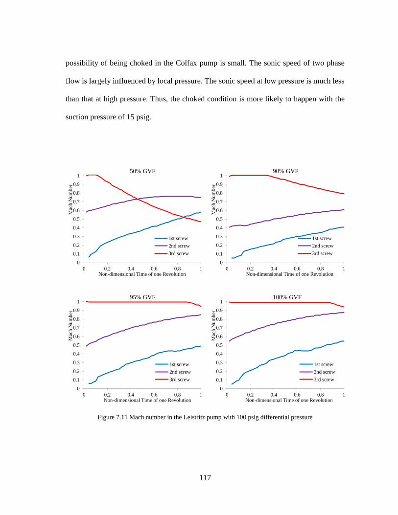
117
possibility of being choked in the Colfax pump is small. The sonic speed of two phase
flow is largely influenced by local pressure. The sonic speed at low pressure is much less
than that at high pressure. Thus, the choked condition is more likely to happen with the
suction pressure of 15 psig.
Figure 7.11 Mach number in the Leistritz pump with 100 psig differential pressure
0
0.1
0.2
0.3
0.4
0.5
0.6
0.7
0.8
0.9
1
0 0.2 0.4 0.6 0.8 1
Mac
h N
um
ber
Non-dimensional Time of one Revolution
50% GVF
1st screw
2nd screw
3rd screw
0
0.1
0.2
0.3
0.4
0.5
0.6
0.7
0.8
0.9
1
0 0.2 0.4 0.6 0.8 1
Mac
h N
um
ber
Non-dimensional Time of one Revolution
90% GVF
1st screw
2nd screw
3rd screw
0
0.1
0.2
0.3
0.4
0.5
0.6
0.7
0.8
0.9
1
0 0.2 0.4 0.6 0.8 1
Mac
h N
um
ber
Non-dimensional Time of one Revolution
95% GVF
1st screw
2nd screw
3rd screw
0
0.1
0.2
0.3
0.4
0.5
0.6
0.7
0.8
0.9
1
0 0.2 0.4 0.6 0.8 1
Mac
h N
um
ber
Non-dimensional Time of one Revolution
100% GVF
1st screw
2nd screw
3rd screw

118
Figure 7.12 Mach number in the Leistritz pump with 250 psig differential pressure
0
0.1
0.2
0.3
0.4
0.5
0.6
0.7
0.8
0.9
1
0 0.2 0.4 0.6 0.8 1
Mac
h N
um
ber
Non-dimensional Time of one Revolution
50% GVF
1st screw
2nd screw
3rd screw
0
0.1
0.2
0.3
0.4
0.5
0.6
0.7
0.8
0.9
1
0 0.2 0.4 0.6 0.8 1
Mac
h N
um
ber
Non-dimensional Time of one Revolution
90% GVF
1st screw
2nd screw
3rd screw
0
0.1
0.2
0.3
0.4
0.5
0.6
0.7
0.8
0.9
1
0 0.2 0.4 0.6 0.8 1
Mac
h N
um
ber
Non-dimensional Time of one Revolution
95% GVF
1st screw
2nd screw
3rd screw
0
0.1
0.2
0.3
0.4
0.5
0.6
0.7
0.8
0.9
1
0 0.2 0.4 0.6 0.8 1
Mac
h N
um
ber
Non-dimensional Time of one Revolution
100% GVF
1st screw
2nd screw
3rd screw

119
Figure 7.13 Mach number in the Colfax pump at 200 psig differential pressure, 15 psig suction pressure
0
0.1
0.2
0.3
0.4
0.5
0.6
0.7
0.8
0.9
1
0 0.2 0.4 0.6 0.8 1
Mac
h N
um
ber
Non-dimensional Time of One Revolution
50% GVF1st screw
2nd screw
3rd screw
4th screw
5th screw
6th screw
7th screw
0
0.1
0.2
0.3
0.4
0.5
0.6
0.7
0.8
0.9
1
0 0.2 0.4 0.6 0.8 1
Mac
h N
um
ber
Non-dimensional Time of One Revolution
70% GVF1st screw
2nd screw
3rd screw
4th screw
5th screw
6th screw
7th screw
0
0.1
0.2
0.3
0.4
0.5
0.6
0.7
0.8
0.9
1
0 0.2 0.4 0.6 0.8 1
Mac
h N
um
ber
Non-dimensional Time of One Revolution
90% GVF1st screw
2nd screw
3rd screw
4th screw
5th screw
6th screw
7th screw
0
0.1
0.2
0.3
0.4
0.5
0.6
0.7
0.8
0.9
1
0 0.2 0.4 0.6 0.8 1
Mac
h N
um
ber
Non-dimensional Time of One Revolution
100% GVF1st screw
2nd screw
3rd screw
4th screw
5th screw
6th screw
7th screw

120
Figure 7.14 Mach number in the Colfax pump at 200 psig differential pressure, 100 psig suction pressure
7.7 Effect of Suction Pressure on Volumetric Efficiency
The suction pressure has an essential effect on the volumetric efficiency when twin
screw pump operated with two phase flow. As shown in Figure 7.15, volumetric
efficiency suffers significant decrease as suction pressure increases from 15 psig to 100
psig indicating less choked flow conditions.
0
0.1
0.2
0.3
0.4
0.5
0.6
0.7
0.8
0.9
1
0 0.2 0.4 0.6 0.8 1
Mac
h N
um
ber
Non-dimensional Time of One Revolution
50% GVF1st screw
2nd screw
3rd screw
4th screw
5th screw
6th screw
7th screw
0
0.1
0.2
0.3
0.4
0.5
0.6
0.7
0.8
0.9
1
0 0.2 0.4 0.6 0.8 1
Mac
h N
um
ber
Non-dimensional Time of One Revolution
70% GVF1st screw
2nd screw
3rd screw
4th screw
5th screw
6th screw
7th screw
0
0.1
0.2
0.3
0.4
0.5
0.6
0.7
0.8
0.9
1
0 0.2 0.4 0.6 0.8 1
Mac
h N
um
ber
Non-dimensional Time of One Revolution
90% GVF1st screw
2nd screw
3rd screw
4th screw
5th screw
6th screw
7th screw
0
0.1
0.2
0.3
0.4
0.5
0.6
0.7
0.8
0.9
1
0 0.2 0.4 0.6 0.8 1
Mac
h N
um
ber
Non-dimensional Time of One Revolution
100% GVF1st screw
2nd screw
3rd screw
4th screw
5th screw
6th screw
7th screw

121
Figure 7.16 shows the comparison of non-dimensional pressure distribution in the
Colfax pump at 15 psig suction pressure and 100 psig suction pressure. It is found that
the pressure distribution becomes more linear with increasing suction pressure. The
pressure drop through the first screw is much larger with 100 psig suction pressure,
which leads to the increased leakage flow rate over the first screw. Meanwhile, the
pressure drop is more over the screws near the discharge side with 15 psig suction
pressure. Because the leakage flow is more inclined to be choked near the discharge side
with 15 psig suction pressure. As shown in Figure 7.13 and Figure 7.14, the choked
condition occurs at the last screw with 90% GVF and 100% GVF with 15 psig suction
pressure, while the Mach number of 100 psig suction pressure is much less.
Figure 7.15 Comparison of volumetric efficiency for Colfax pump with different suction pressure
(experimental data)
0.6
0.65
0.7
0.75
0.8
0.85
0.9
0.95
1
0 50 100 150 200 250 300
Vo
lum
etri
c E
ffic
iency
Differential Pressure (psig)
Inlet P = 15 psig, 50% GVF
Inlet P = 15 psig, 70% GVF
Inlet P = 15 psig, 90% GVF
Inlet P = 15 psig, 100% GVF
Inlet P = 100 psig, 50% GVF
Inlet P = 100 psig, 70% GVF
Inlet P = 100 psig, 90% GVF
Inlet P = 100 psig, 100% GVF

122
Figure 7.16 Comparison of pressure distribution for Colfax pump with different suction pressure
Figure 7.17 Comparison of water/air sonic speed at 100 psig and 15 psig
0
0.1
0.2
0.3
0.4
0.5
0.6
0.7
0.8
0.9
1
1 2 3 4 5 6 7 8
No
n-d
imen
sio
nal
Pre
ssure
Position, Inlet to Outlet
pressure distribution
Inlet P = 15 psig, 50% GVF
Inlet P = 15 psig, 70% GVF
Inlet P = 15 psig, 100% GVF
Inlet P = 100 psig, 50% GVF
Inlet P = 100 psig, 70% GVF
Inlet P = 100 psig, 100% GVF
0
100
200
300
400
500
600
0 20 40 60 80 100
So
nic
Sp
eed
(m
/s)
GVF (%)
sonic speed at 100 psigsonic speed at 15 psig

123
7.8 Effect of Water Cut on Pump Performance
Experimental test data shows that the volumetric efficiency of the oil and nitrogen test is
lower than that of the water and air test for all testing conditions. As shown in Figure
7.18 and Figure 7.19, the prediction data also arrives at the same conclusion. Though the
viscosity of oil is higher than the viscosity of water, the leakage flow rate of the oil test
is larger than the leakage flow rate of water test. Previous experimental result also shows
the same trend. Chan [6] found that efficiency doesn’t increase with the increase of
viscosity from 1 cp to 10 cP.
As show in Figure 7.20, the Mach number distribution of the oil test and the water test
are almost the same. However, the sonic speed of oil and nitrogen mixture is larger than
the sonic speed of water and air mixture. As result, the velocity of oil and nitrogen flow
is larger than the velocity of water and air flow in the clearance, which leads to a larger
leakage flow rate of oil test.
Hence, the friction loss in the clearance isn’t the main factor to determine the leakage
flow rate for the low viscosity flow. Instead, the pressure loss due to the expansion of
two phase flow in the clearance has a larger effect on the leakage flow rate. Thus, though
the viscosity of the oil is larger than the viscosity of water, the volumetric efficiency of
oil/ nitrogen test is lower than the volumetric efficiency of water/ air test.

124
Figure 7.18 Prediction comparison of volumetric efficiency of water test and oil test at 3550 RPM
Figure 7.19 Prediction comparison of volumetric efficiency of water test and oil test at 4000 RPM
0
0.1
0.2
0.3
0.4
0.5
0.6
0.7
0.8
0.9
1
0 200 400 600 800 1000
Vo
lum
etri
c E
ffic
iency
Differential Pressure (psig)
3550 RPM, comparison
30% GVF water test
50% GVF water test
85% GVF water test
30% GVF oil test
50% GVF oil test
85% GVF oil test
0
0.1
0.2
0.3
0.4
0.5
0.6
0.7
0.8
0.9
1
0 200 400 600 800 1000
Vo
lum
etri
c E
ffic
iency
Differential Pressure (psig)
4000 RPM, comparison
30% GVF water test
50% GVF water test
85% GVF water test
30% GVF oil test
50% GVF oil test
85% GVF oil test

125
Figure 7.20 Comparison of Mach number for Can-K pump of water test and oil test at 4000 RPM, 1000
psig differential pressure, 50% GVF
Figure 7.21 Comparison of sonic speed of water/ air and oil/ nitrogen at 100 psig
0
0.1
0.2
0.3
0.4
0.5
0 0.2 0.4 0.6 0.8 1
Mac
h N
um
ber
Non-dimensional Time in a Revolution
1st screw water test
2nd screw water test
3rd screw water test
4th screw water test
1st screw oil test
2nd screw oil test
3rd screw oil test
4th screw oil test
0
50
100
150
200
250
300
350
400
450
500
0 20 40 60 80 100
So
nic
Sp
eed
(m
/s)
GVF (%)
sonic speed of water&air
sonic speed of oil&nitrogen

126
8 CONCLUSION
8.1 Experimental
In this research, the multiphase performance of a multistage twin screw pump has been
investigated. Water-air mixture, oil-nitrogen mixture and oil-water-nitrogen mixture
were selected as working fluids. The pump was tested with different differential
pressures and different pump speeds. The GVF at the pump inlet varies from 0% to 85%.
While water cut values of 0%, 50%, 80% and 100% were used.
Experimental results show that the curve of pressure distribution along the stages
changes from concave-down to concave-up with the increase of GVF from 10% to 85%
at the same differential pressure.
The volumetric efficiency increases as the GVF increases. The volumetric efficiency
decreases with the increase of differential pressure. The volumetric efficiency of the oil
test is lower than water test.
It is found the mechanical efficiency increases with the increase of differential pressure
when the differential pressure is small. The mechanical efficiency decreases with the
increase of differential pressure when the differential pressure is large. The mechanical
efficiency becomes the maximum at about 600 psig differential pressure.

127
Compared with the single stage twin screw pump, the mechanical efficiency of Can-K
pump is much lower. This is because the multistage pump has to overcome larger
friction losses.
8.2 Analytical Model
An analytical model has been developed using MATLAB to predict the multiphase
performance of twin screw pumps. A two phase Fanno flow model is used to model the
leakage flow in the clearance. The compressibility of the leakage flow has been
investigated.
The analytical model has been employed to predict the multiphase performance of
various twin screw pumps. It has been demonstrated that the predictions match the
experimental data well with the GVF ranging from 20% to 100% for the single stage
pumps. A new method has been proposed to predict the multiphase performance of
multistage twin screw pump. And it has been used to predict the performance of the
Can-K pump with the GVF ranging from 10% to 85%.
The prediction shows that the GVF has a significant effect on the pressure distribution
along the screws. With an increase of the GVF, the shape of the pressure distribution
becomes steeper at the discharge side.
The possibility of choked flow condition has been investigated in this research. It is
found the leakage flow is more likely to be choked with high differential pressure flow
conditions. Besides, the sonic speed of two phase flow increases with the increase of the

128
local pressure. As a result, the choked condition is more likely to occur with low suction
pressure conditions.
The Can-K pump shows different performance with different water cut. The volumetric
efficiency increases with increasing water cut. Since the viscosity of the oil is very close
to the viscosity of water. The viscosity isn’t the dominant factor to determine the leakage
flow rate. The sonic speed of the oil and nitrogen flow is higher than that of water and
air flow. Thus the leakage flow of the oil and nitrogen has a higher velocity with the
same Mach number, which leads to a lower volumetric efficiency.
8.3 Recommendations
In this research, the multiphase performance of a multistage twin screw pump has been
investigated. However, the pump was tested with only one suction pressure. The effect
of different suction pressure has not been investigated on the Can-K pump. Besides, a
low viscosity oil was used as working fluid. The performance of the pump working with
high viscosity oil hasn’t been studied.
For the analytical model, the pressure distribution of the multistage pump is obtained by
an empirical equation. New methods are still need to be developed to analyze the
pressure distributions along the stages for the multistage pump.

129
REFERENCES
[1] Schlumberger. (2016, January 30). Integrated Lifting Solutions for Enhanced well
Production. Retrieved from http://www.slb.com/services/production/artificial_lift.aspx
[2] Fleshman, R., and Lekic, H. "Artificial Lift for High-Volume Production." Oilfield
Review, Spring 1999. 49-63.
[3] Zheng, D. Three Phase Erosion Testing and Vibration Analysis of an Electrical
Submersible Pump. MSc Thesis, College Station: Texas A&M University, 2013.
[4] Dass, P. "Twin-Screw Pumps rival Traditional Artificial Lift Systems." E&P, 2009.
76-77.
[5] Karassik, I., Messina, J., Cooper, P., and Heald, C. Pump Handbook (3rd edition).
McGRAW-HILL, New York, 2001. 3.99-3.122.
[6] Chan, E. Wet-gas compression in twin-screw multiphase pumps. MS Thesis, College
Station: Texas A&M University, 2006.
[7] Vetter, G., and Wincek, M. "Performance Prediction of Twin-Screw pumps for Two-
Phase Gas/Liquid Flow." Pumping Machinery, ASME, Fluid Engineering Conference
(FED). Washington, D.C: ASME, 1993. 331-340.
[8] Egashira, K., Shoda, S., Tochikawa, T., and Furukawa, A. "Backflow in Twin-
Screw-Type Multiphase Pump." SPEPF, 1998. 64-69.

130
[9] Feng, C., Yueyuan, P., Ziwen, X., and Pengcheng, S. "Thermodynamic performance
simulation of a twin-screw multiphase pump." Journal of Process Mechanical
Engineering , 2001. 157-162.
[10] Nakashima, C., Oliveira, S., and Caetano, E. "Thermodynamic Model of a Twin-
Screw Multiphase Pump." Proceedings of ETCE, 2002. 877-885.
[11] Martin, A.M. Multiphase Twin Screw Pump Modeling for Oil and Gas Industry.
PhD Thesis, College Station: Texas A&M University, 2003.
[12] Prang, A., and Cooper, P. "Enhanced Multiphase Flow Prediction in Twin-Screw
Pumps." Proceedings of the 21th International Pump Users Symposium, 2004. 69-76.
[13] Rausch, T., Vauth, Th., Brandt, J-U., and Mewes, D. "A Model for the Delivering
Characteristic of Multiphase pumps." 4th Conference on Multiphase Technology, Banff,
Canada, 2004. 313-327.
[14] Vetter, G., Wirth, W., Korner, H., and Pregler. "Multiphase Pumping with Twin-
Screw pumps - Understand and Model Hydrodynamics and Hydroabrasive Wear." 7th
International Pump User Symposium, Turbomachinery Laboratory. Houston, Texas
A&M University, 2000. 153-169.
[15] Nakashima, C., Oliveira, S., and Caetano, E. "Thermo-Hydraulic Model of a Twin-
Screw Multiphase Pump." Proceedings of IMECE04, 2004. 251-260
[16] Xu, J. Modelling of Wet Gas Compression in Twin Screw Multiphase Pump. PhD
Thesis, College Station: Texas A&M University, 2008.
131
[17] Rabiger, K., Maksoud, T., and Ward, J. "Thermo- and Fluid Dynamic Model of a
Multiphase Screw Pump, Operating at Very High Gas Volume Fractions." Schriftenreihe
der Georg-Simon-Ohm-Fachhochschule Nurnberg. Nr.35, November 2006.
[18] Rabiger, K., Maksoud, T., Ward, J., and Hausmann, G. "Investigation of the Fluid
Dynamic and Thermodynamic Behaviour of Multiphase Screw Pumps Handling
Liquid/gas Mixtures with Very High Gas Volume Fractions." BHR Group 2007
Multiphase Production Technology 13. 91-104.
[19] Rabiger, K., Maksoud, T., Ward, J., and Hausmann, G. "Theoretical and
Experimental Analysis of a Multiphase Screw Pump, Handling Gas-Liquid Mixtures
with Very High Gas Volume Fractions." Experimental Thermal and Fluid Science
32(2008). 1694-701.
[20] Rabiger, K. Fluid Dynamic and Thermodynamic Behaviour of Multiphase Screw
Pumps Handling Gas-Liquid Mixtures with Very High Gas Volume Fractions. PhD
Thesis, Nuremberg: University of Applied Sciences in Nuremberg, 2009.
[21] Kroupa, R. Investigation of a Multiphase Twin-screw Pump Operating at High Gas
Volume Fractions. MSc Thesis, College Station: Texas A&M University, 2011.
[22] Morrison, G., Kroupa, R., Patil, A., Xu, J., Scott, S., and Olson, S. "Experimental
Investigation of Wellhead Twin-Screw Pump for Gas-Well Deliquefication." Oil and
Gas Facilities Journal, SPE, April 2014. 73-80.

132
[23] Patil, A. R. Performance Evaluation and CFD Simulation of Multiphase Twin-
Screw Pumps. Ph.D. Dissertation, College Station: Texas A&M University, 2013.
[24] Morrison, G., Patil, A., and Cihak, D. "Evaluation of a Twin Screw Pump for Use in
High Gas Volume Fraction Flows." ASME Fluids Engineering Summer Meeting, Puerto
Rico, 2012. 1-9
[25] Turhan, Y. Efficiency and Leakage Analysis of a Twin-Screw Multiphase Pump.
MSc Thesis, College Station: Texas A&M University, 2014.
[26] Brennen, C. E. Fundamentals of Multiphase Flow. Cambridge University Press,
Pasadena, 2005. 220-246.
[27] Morrison, G., Patil, A., and Cihak, D. "Efficiency limit for multiphase pumps." 8th
North American Conference on Multiphase Technology (BHR Group), Banff, Canada,
20-22 June, 2012. 17-29.

133
APPENDIX A
UNCERTAINTY ANALYSIS
A.1 Water Cut
The water cut is calculated based on the mixture density which is measured by the
Coriolis flow meter,
𝜂𝑤 =𝜌𝑚 − 𝜌𝑜
𝜌𝑤 − 𝜌𝑜
A.1
Thus the uncertainty of the water cut is calculated with the following equation,
𝑢𝜂𝑤= [(
𝜕𝜂𝑤
𝜕𝜌𝑚𝑢𝜌𝑚
)2
]
0.5
A.2
Which simplifies to,
𝜇𝜂𝑤=
1
𝜌𝑤 − 𝜌𝑜𝜇𝜌𝑚
A.3
The measurement uncertainty of density is shown in Table 4.4. The uncertainty of 50%
water cut and 80% water cut is given in Table A.1.
Table A.1 Uncertainty of Water Cut
Water Cut (%) 𝑢𝜂𝑤 (%) 𝑢𝜂𝑤
𝜂𝑤⁄ (%)
50 0.28 0.56
80 0.28 0.35
A.2 Liquid Flow Rate
For the water/oil test, it is found that the separator can’t separate the gas and liquid
thoroughly. There is some gas mixed in the liquid line, which leads to the measurement

134
error of the liquid flow rate. The liquid flow rate is calibrated with the following
equation,
𝑄𝑙 = 𝑄𝑙′
𝜌𝑚 − 𝜌𝑔
𝜌𝑙 − 𝜌𝑔 A.4
𝜌𝑚 is the density measured by the liquid flow meter. Thus,
𝜇𝑄𝑙= [(
𝜕𝑄𝑙
𝜕𝑄𝑙′𝜇𝑄𝑙′
)2
+ (𝜕𝑄𝑙
𝜕𝜌𝑚𝜇𝜌𝑚
)2
+ (𝜕𝑄𝑙
𝜕𝜌𝑔𝜇𝜌𝑔
)
2
]
0.5
A.5
The density of the gas is given by the following equation,
𝜌𝑔 =𝑝
𝑅𝑝 A.6
Thus the uncertainty of the gas density is,
𝜇𝜌𝑔= [(
𝜕𝜌𝑔
𝜕𝑝𝜇𝑝)
2
+ (𝜕𝜌𝑔
𝜕𝑇𝜇𝑇)
2
]
0.5
A.7
The uncertainties of the liquid flow rate are presented in Table A.2.
Table A.2 Uncertainty of Liquid Flow Rate for 100% water cut test at 4000 RPM
GVF (%) dP (psi) 𝑄𝑙 (gpm) 𝜇𝑄𝑙 (gpm) 𝜇𝑄𝑙
𝑄𝑙⁄ (%)
50 200 42.184 0.047 0.11
50 1000 28.187 0.032 0.11
A.3 Gas Flow Rate at the Pump Inlet
The gas flow rate at the pump inlet is calculated with the air flow rate at the flow meters
with the following equation,
𝑄𝑔 = 𝑄𝑔′
𝑝0𝑇𝑖
𝑝𝑖𝑇0+ 𝑄𝑙′
𝜌𝑙 − 𝜌𝑚
𝜌𝑙 − 𝜌𝑔 A.8
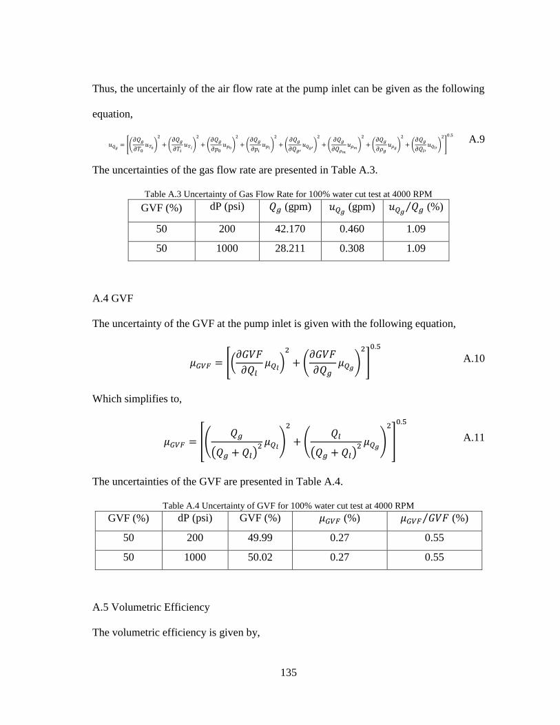
135
Thus, the uncertainly of the air flow rate at the pump inlet can be given as the following
equation,
𝑢𝑄𝑔
= [(𝜕𝑄𝑔
𝜕𝑇0𝑢𝑇0
)
2
+ (𝜕𝑄𝑔
𝜕𝑇𝑖𝑢𝑇𝑖
)
2
+ (𝜕𝑄𝑔
𝜕𝑝0𝑢𝑝0
)
2
+ (𝜕𝑄𝑔
𝜕𝑝𝑖𝑢𝑝𝑖
)
2
+ (𝜕𝑄𝑔
𝜕𝑄𝑔′𝑢𝑄𝑔′
)
2
+ (𝜕𝑄𝑔
𝜕𝑄𝜌𝑚
𝑢𝜌𝑚)
2
+ (𝜕𝑄𝑔
𝜕𝜌𝑔𝑢𝜌𝑔
)
2
+ (𝜕𝑄𝑔
𝜕𝑄𝑙′𝑢𝑄𝑙′
)
2
]
0.5
A.9
The uncertainties of the gas flow rate are presented in Table A.3.
Table A.3 Uncertainty of Gas Flow Rate for 100% water cut test at 4000 RPM
GVF (%) dP (psi) 𝑄𝑔 (gpm) 𝑢𝑄𝑔 (gpm) 𝑢𝑄𝑔
𝑄𝑔⁄ (%)
50 200 42.170 0.460 1.09
50 1000 28.211 0.308 1.09
A.4 GVF
The uncertainty of the GVF at the pump inlet is given with the following equation,
𝜇𝐺𝑉𝐹 = [(𝜕𝐺𝑉𝐹
𝜕𝑄𝑙𝜇𝑄𝑙
)2
+ (𝜕𝐺𝑉𝐹
𝜕𝑄𝑔𝜇𝑄𝑔
)
2
]
0.5
A.10
Which simplifies to,
𝜇𝐺𝑉𝐹 = [(𝑄𝑔
(𝑄𝑔 + 𝑄𝑙)2 𝜇𝑄𝑙
)
2
+ (𝑄𝑙
(𝑄𝑔 + 𝑄𝑙)2 𝜇𝑄𝑔
)
2
]
0.5
A.11
The uncertainties of the GVF are presented in Table A.4.
Table A.4 Uncertainty of GVF for 100% water cut test at 4000 RPM
GVF (%) dP (psi) GVF (%) 𝜇𝐺𝑉𝐹 (%) 𝜇𝐺𝑉𝐹 𝐺𝑉𝐹⁄ (%)
50 200 49.99 0.27 0.55
50 1000 50.02 0.27 0.55
A.5 Volumetric Efficiency
The volumetric efficiency is given by,

136
𝜂𝑣 =
𝑄𝑔 + 𝑄𝑙
𝑄𝑡ℎ A.12
Thus, the uncertainty of the volumetric efficiency is given with the following equation,
𝜇𝜂𝑣= [(
𝜕𝜂𝑣
𝜕𝑄𝑔𝜇𝑄𝑔
)
2
+ (𝜕𝜂𝑣
𝜕𝑄𝑙𝜇𝑄𝑙
)2
]
0.5
A.13
Which simplifies to,
𝜇𝜂𝑣
=1
𝑄𝑡ℎ[(𝜇𝑄𝑔
)2
+ (𝜇𝑄𝑙)
2]
0.5
A.14
The uncertainties of the volumetric efficiency are presented in Table A.5.
Table A.5 Uncertainty of Volumetric Efficiency for 100% water cut test at 4000 RPM
GVF (%) dP (psi) 𝜂𝑣 (%) 𝜇𝜂𝑣 (%) 𝜇𝜂𝑣
𝜂𝑣⁄ (%)
50 200 0.743 0.0041 0.55
50 1000 0.497 0.0027 0.55
A.6 Polytropic Coefficient
The polytropic coefficient is given by,
𝑛 =𝐼𝑛 (
𝑝𝑖𝑛
𝑝𝑜𝑢𝑡)
𝐼𝑛 (𝑝𝑖𝑛
𝑝𝑜𝑢𝑡∙
𝑇𝑜𝑢𝑡
𝑇𝑖𝑛) A.15
The uncertainty of the polytropic coefficient is given with the following equation,
𝜇𝑛 = [(𝜕𝑛
𝜕𝑝𝑖𝑛𝜇𝑝𝑖𝑛
)2
+ (𝜕𝑛
𝜕𝑝𝑜𝑢𝑡𝜇𝑝𝑜𝑢𝑡
)2
+ (𝜕𝑛
𝜕𝑇𝑖𝑛𝜇𝑇𝑖𝑛
)2
+ (𝜕𝑛
𝜕𝑇𝑜𝑢𝑡𝜇𝑇𝑜𝑢𝑡
)2
]
0.5
A.16
The uncertainties of the polytropic coefficient are presented in Table A.6.
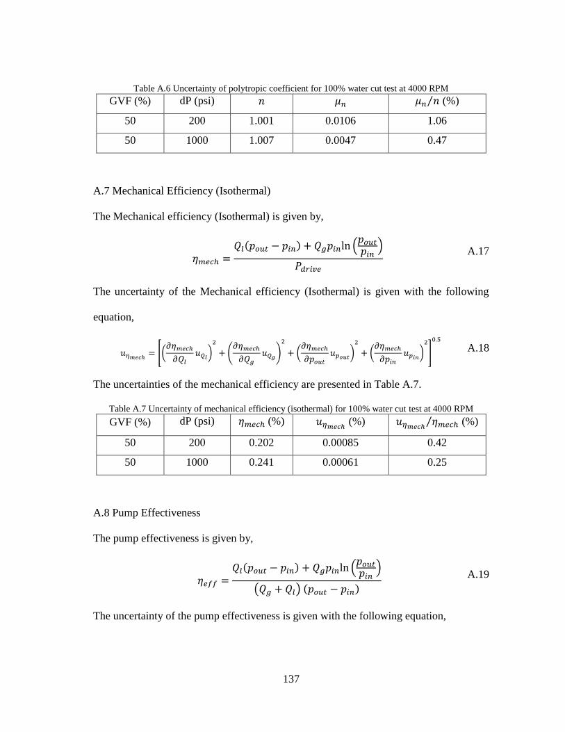
137
Table A.6 Uncertainty of polytropic coefficient for 100% water cut test at 4000 RPM
GVF (%) dP (psi) 𝑛 𝜇𝑛 𝜇𝑛 𝑛⁄ (%)
50 200 1.001 0.0106 1.06
50 1000 1.007 0.0047 0.47
A.7 Mechanical Efficiency (Isothermal)
The Mechanical efficiency (Isothermal) is given by,
𝜂𝑚𝑒𝑐ℎ =𝑄𝑙(𝑝𝑜𝑢𝑡 − 𝑝𝑖𝑛) + 𝑄𝑔𝑝𝑖𝑛ln (
𝑝𝑜𝑢𝑡
𝑝𝑖𝑛)
𝑃𝑑𝑟𝑖𝑣𝑒
A.17
The uncertainty of the Mechanical efficiency (Isothermal) is given with the following
equation,
𝑢𝜂𝑚𝑒𝑐ℎ
= [(𝜕𝜂𝑚𝑒𝑐ℎ
𝜕𝑄𝑙
𝑢𝑄𝑙)
2
+ (𝜕𝜂𝑚𝑒𝑐ℎ
𝜕𝑄𝑔
𝑢𝑄𝑔)
2
+ (𝜕𝜂𝑚𝑒𝑐ℎ
𝜕𝑝𝑜𝑢𝑡
𝑢𝑝𝑜𝑢𝑡)
2
+ (𝜕𝜂𝑚𝑒𝑐ℎ
𝜕𝑝𝑖𝑛
𝑢𝑝𝑖𝑛)
2
]
0.5
A.18
The uncertainties of the mechanical efficiency are presented in Table A.7.
Table A.7 Uncertainty of mechanical efficiency (isothermal) for 100% water cut test at 4000 RPM
GVF (%) dP (psi) 𝜂𝑚𝑒𝑐ℎ (%) 𝑢𝜂𝑚𝑒𝑐ℎ (%) 𝑢𝜂𝑚𝑒𝑐ℎ
𝜂𝑚𝑒𝑐ℎ⁄ (%)
50 200 0.202 0.00085 0.42
50 1000 0.241 0.00061 0.25
A.8 Pump Effectiveness
The pump effectiveness is given by,
𝜂𝑒𝑓𝑓 =𝑄𝑙(𝑝𝑜𝑢𝑡 − 𝑝𝑖𝑛) + 𝑄𝑔𝑝𝑖𝑛ln (
𝑝𝑜𝑢𝑡
𝑝𝑖𝑛)
(𝑄𝑔 + 𝑄𝑙) (𝑝𝑜𝑢𝑡 − 𝑝𝑖𝑛)
A.19
The uncertainty of the pump effectiveness is given with the following equation,

138
𝜇𝜂𝑒𝑓𝑓
= [(𝜕𝜂𝑒𝑓𝑓
𝜕𝑝𝑖𝑛
𝜇𝑝𝑖𝑛)
2
+ (𝜕𝜂𝑒𝑓𝑓
𝜕𝑝𝑜𝑢𝑡
𝜇𝑝𝑜𝑢𝑡)
2
+ (𝜕𝜂𝑒𝑓𝑓
𝜕𝑄𝑙
𝜇𝑄𝑙)
2
+ (𝜕𝜂𝑒𝑓𝑓
𝜕𝑄𝑔
𝜇𝑄𝑔)
2
]
0.5
A.20
The uncertainties of the pump effectiveness are presented in Table A.8.
Table A.8 Uncertainty of Liquid Flow Rate for 100% water cut test at 4000 RPM
GVF (%) dP (psi) 𝜂𝑒𝑓𝑓(%) 𝜇𝜂𝑒𝑓𝑓 (%) 𝜇𝜂𝑒𝑓𝑓
𝜂𝑒𝑓𝑓⁄ (%)
50 200 0.791 0.0012 0.15
50 1000 0.631 0.002 0.32
Related Documents