Performance-Estimation Properties of Cross-Validation- Based Protocols with Simultaneous Hyper-Parameter Optimization Ioannis Tsamardinos 1,2 , Amin Rakhshani 1,2 ,Vincenzo Lagani 1 1 Institute of Computer Science, Foundation for Research and Technology Hellas, Heraklion, Greece 2 Computer Science Department, University of Crete, Heraklion, Greece { tsamard, vlagani, aminra }@ics.forth.gr Abstract. In a typical supervised data analysis task, one needs to perform the following two tasks: (a) select the best combination of learning methods (e.g., for variable selection and classifier) and tune their hyper-parameters (e.g., K in K-NN), also called model selection, and (b) provide an estimate of the perfor- mance of the final, reported model. Combining the two tasks is not trivial be- cause when one selects the set of hyper-parameters that seem to provide the best estimated performance, this estimation is optimistic (biased / overfitted) due to performing multiple statistical comparisons. In this paper, we confirm that the simple Cross-Validation with model selection is indeed optimistic (overesti- mates) in small sample scenarios. In comparison the Nested Cross Validation and the method by Tibshirani and Tibshirani provide conservative estimations, with the later protocol being more computationally efficient. The role of strati- fication of samples is examined and it is shown that stratification is beneficial. 1 Introduction A typical supervised analysis (e.g., classification or regression) consists of several steps that result in a final, single prediction, or diagnostic model. For example, the analyst may need to impute missing values, perform variable selection or general dimensionality reduction, discretize variables, try several different representations of the data, and finally, apply a learning algorithm for classification or regression. Each of these steps requires a selection of algorithms out of hundreds or even thousands of possible choices, as well as the tuning of their hyper-parameters 1 . Hyper-parameter 1 We use the term “hyper-parameters” to denote the algorithm parameters that can be set by the user and are not estimated directly from the data, e.g., the parameter K in the K-NN algo- rithm. In contrast, the term “parameters” in the statistical literature typically refers to the

Welcome message from author
This document is posted to help you gain knowledge. Please leave a comment to let me know what you think about it! Share it to your friends and learn new things together.
Transcript
Performance-Estimation Properties of Cross-Validation-
Based Protocols with Simultaneous Hyper-Parameter
Optimization
Ioannis Tsamardinos1,2 , Amin Rakhshani 1,2 ,Vincenzo Lagani1
1Institute of Computer Science, Foundation for Research and Technology Hellas, Heraklion,
Greece 2Computer Science Department, University of Crete, Heraklion, Greece
{ tsamard, vlagani, aminra }@ics.forth.gr
Abstract. In a typical supervised data analysis task, one needs to perform the
following two tasks: (a) select the best combination of learning methods (e.g.,
for variable selection and classifier) and tune their hyper-parameters (e.g., K in
K-NN), also called model selection, and (b) provide an estimate of the perfor-
mance of the final, reported model. Combining the two tasks is not trivial be-
cause when one selects the set of hyper-parameters that seem to provide the best
estimated performance, this estimation is optimistic (biased / overfitted) due to
performing multiple statistical comparisons. In this paper, we confirm that the
simple Cross-Validation with model selection is indeed optimistic (overesti-
mates) in small sample scenarios. In comparison the Nested Cross Validation
and the method by Tibshirani and Tibshirani provide conservative estimations,
with the later protocol being more computationally efficient. The role of strati-
fication of samples is examined and it is shown that stratification is beneficial.
1 Introduction
A typical supervised analysis (e.g., classification or regression) consists of several
steps that result in a final, single prediction, or diagnostic model. For example, the
analyst may need to impute missing values, perform variable selection or general
dimensionality reduction, discretize variables, try several different representations of
the data, and finally, apply a learning algorithm for classification or regression. Each
of these steps requires a selection of algorithms out of hundreds or even thousands of
possible choices, as well as the tuning of their hyper-parameters1. Hyper-parameter
1 We use the term “hyper-parameters” to denote the algorithm parameters that can be set by
the user and are not estimated directly from the data, e.g., the parameter K in the K-NN algo-
rithm. In contrast, the term “parameters” in the statistical literature typically refers to the

optimization is also called the model selection problem since each combination of
hyper-parameters tried leads to a possible classification or regression model out of
which the best is to be selected.
There are several alternatives in the literature about how to identify a good combi-
nation of methods and their hyper-parameters (e.g., [1][2]) and they all involve im-
plicitly or explicitly searching the space of hyper-parameters and trying different
combinations. Unfortunately, trying multiple combinations, estimating their perfor-
mance, and reporting the performance of the best model found leads to overestimating
the performance (i.e., underestimate the error / loss), sometimes also referred to as
overfitting2. This phenomenon is called the problem of multiple comparisons in in-
duction algorithms and has been analyzed in detail in [3] and is related to the multiple
testing or multiple comparisons in statistical hypothesis testing. Intuitively, when one
selects among several models whose estimations vary around their true mean value, it
becomes likely that what seems to be the best model has been “lucky” in the specific
test set and its performance has been overestimated. Extensive discussions and exper-
iments on the subject can be found in [2].
The bias should increase with the number of models tried and decrease with the size
of the test set. Notice that, when using Cross Validation-based protocols to estimate
performance each sample serves once and only once as a test case. Thus, one can
consider the total data-set sample size as the size of the test set. Typical high-
dimensional datasets in biology often contain less than 100 samples and thus, one
should be careful with the estimation protocols employed for their analysis.
What about the number of different models tried in an analysis? Is it realistic to ex-
pect an analyst to generate thousands of different models? Obviously, it is very rare
that any analyst will employ thousands of different algorithms; however, most learn-
ing algorithms are parameterized by several different hyper-parameters. For example,
the standard 1-norm, polynomial Support Vector Machine algorithm takes as hyper-
parameters the cost C of misclassifications and the degree of the polynomial d. Simi-
larly, most variable selection methods take as input a statistical significance threshold
or the number of variables to return. If an analyst tries several different methods for
imputation, discretization, variable selection, and classification, each with several
different hyper-parameter values, the number of combinations explodes and can easily
reach into the thousands.
model quantities that are estimated directly by the data, e.g., the weight vector w in a linear
regression model y = w• x + b. See [2] for a definition and discussion too. 2 The term “overfitting” is a more general term and we prefer the term “overestimating” to
characterize this phenomenon.
Notice that, model selection and optimistic estimation of performance may also
happen unintentionally and implicitly in many other settings. More specifically, con-
sider a typical publication where a new algorithm is introduced and its performance
(after tuning the hyper-parameters) is compared against numerous other alternatives
from the literature (again, after tuning their hyper-parameters), on several datasets.
The comparison aims to comparatively evaluate the methods. However, the reported
performances of the best method on each dataset suffer from the same problem of
multiple inductions and are on average optimistically estimated.
In the remainder of the paper, we revisit the Cross-Validation (CV) protocol. We
corroborate [2][4] that CV overestimates performance when it is used with hyper-
parameter optimization. As expected overestimation of performance increases with
decreasing sample sizes. We present two other performance estimation methods in the
literature. The method by Tibshirani and Tibshirani (hereafter TT) [5] tries to estimate
the bias and remove it from the estimation. The Nested Cross Validation (NCV)
method [6] cross-validates the whole hyper-parameter optimization procedure (which
includes an inner cross-validation, hence the name). NCV is a generalization of the
technique where data is partitioned in train-validation-test sets. We show that both of
them are conservative (underestimate) performance, while TT is computationally
more efficient. To our knowledge, this is the first time the three methods are com-
pared against each other on real datasets. The excellent behavior of TT in these pre-
liminary results makes it a promising alternative to NCV.
The effect of stratification is also empirically examined. Stratification is a technique
that during partitioning of the data into folds for cross-validation forces the same dis-
tribution of the outcome classes to each fold. When data are split randomly, on aver-
age, the distribution of the outcome in each fold will be the same as in the whole da-
taset. However, in small sample sizes or imbalanced data it could happen that a fold
gets no samples that belong in one of the classes (or in general, the class distribution
in a fold is very different from the original). Stratification ensures that this doesn’t
occur. We show that stratification decreases the variance of the estimation and thus
should always be applied.
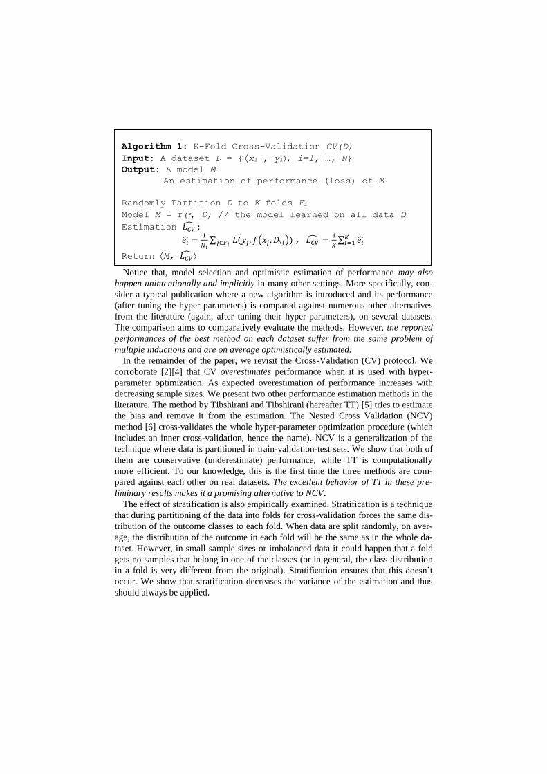
Algorithm 1: K-Fold Cross-Validation CV(D)
Input: A dataset D = {xi , yi, i=1, …, N}
Output: A model M
An estimation of performance (loss) of M
Randomly Partition D to K folds Fi
Model M = f(•, D) // the model learned on all data D Estimation 𝐿𝐶�̂�:
𝑒�̂� =1
𝑁𝑖∑ 𝐿(𝑦𝑗 , 𝑓(𝑥𝑗 , 𝐷\𝑖))𝑗∈𝐹𝑖
, 𝐿𝐶�̂� =1
𝐾∑ 𝑒�̂�
𝐾𝑖=1
Return M, 𝐿𝐶�̂�
2 Cross-Validation Without Hyper-Parameter Optimization
(CV)
K-fold Cross Validation is perhaps the most common method for estimating perfor-
mance of a learning method for small and medium sample sizes. Despite its populari-
ty, its theoretical properties are arguably not well known especially outside the ma-
chine learning community, particularly when it is employed with simultaneous hyper-
parameter optimization, as evidenced by the following common machine learning
books: Duda ([7], p. 484) presents CV without discussing it in the context of model
selection and only hints that it may underestimate (when used without model selec-
tion): “The jackknife [i.e., leave-one-out CV] in particular, generally gives good esti-
mates because each of the n classifiers is quite similar to the classifier being tested
…”. Similarly, Mitchell [8](pp. 112, 147, 150) mentions CV but in the context of
hyper-parameter optimization. Bishop [9] does not deal at all with issues of perfor-
mance estimation and model selection. A notable exception is the Hastie and co-
authors [10] book that offers the best treatment of the subject, upon which the follow-
ing sections are based. Yet, CV is still not discussed in the context of model selec-
tion.
Let’s assume a dataset D = {xi , yi, i=1, …, N}, of identically and independently
distributed (i.i.d.) predictor vectors xi and corresponding outcomes yi . Let us also
assume that we have a single method for learning from such data and producing a
single prediction model. We will denote with f(xi , D) the output of the model pro-
duced by the learner f when trained on data D and applied on input xi . The actual
model produced by f on dataset D is denoted with f(•, D). We will denote with L(y, y’)
the loss (error) measure of prediction y’ when the true output is y. One common loss
function is the zero-one loss function: L(y, y’) = 1, if yy’ and L(y, y’) = 0, otherwise.
Thus, the average zero-one loss of a classifier equals 1-accuracy, i.e., it is the prob-
ability of making an incorrect classification. K-fold CV partitions the data D into K
subsets called folds F1 , …, Fk . We denote with D\i the data excluding fold Fi and Ni
the sample size of each fold. The K-fold CV algorithm is shown in Algorithm 1.
First, notice that CV returns the model learned from all data D, f(•, D). This is the
model to be employed operationally for classification. It then tries to estimate the
performance of the returned model by constructing K other models from datasets D\i ,
each time excluding one fold from the training set. Each of these models is then ap-
plied on each fold Fi serving as test and the loss is averaged over all samples.
Is 𝐿𝐶�̂� an unbiased estimate of the loss of f(•, D)? First, notice that each sample xi is
used once and only once as a test case. Thus, effectively there are as many i.i.d. test
cases as samples in the dataset. Perhaps, this characteristic is what makes the CV so
popular versus other protocols such as repeatedly partitioning the dataset to train-test
subsets. The test size being as large as possible could facilitate the estimation of the
loss and its variance (although, theoretical results show that there is no unbiased esti-
mator of the variance for the CV! [11]). However, test cases are predicted with differ-
ent models! If these models were trained on independent train sets of size equal to the
original data D, then CV would indeed estimate the average loss of the models pro-

duced by the specific learning method on the specific task when trained with the spe-
cific sample size. As it stands though, since the models are correlated and have small-
er size than the original:
K-Fold CV estimates the average loss of models returned by the specific learning
method f on the specific classification task when trained with subsets of D of size
|D\i|
Since |D\i| = (K-1)/K • |D| < |D| (e.g., for 5-fold, we are using 80% of the total sample
size for training each time) and assuming that the learning method improves on aver-
age with larger sample sizes we expect 𝐿𝐶�̂� to be conservative (i.e., the true perfor-
mance be underestimated). How conservative it will be depends on where the classifi-
er is operating on its learning curve for this specific task. It also depends on the num-
ber of folds K: the larger the K, the more (K-1)/K approaches 100% and the bias dis-
appears, i.e., leave-one-out CV should be the least biased (however, there may be still
be significant estimation problems, see [12], p. 151, and [4] for an extreme failure of
leave-one-out CV). When sample sizes are small or distributions are imbalanced (i.e.,
some classes are quite rare in the data), we expect most classifiers to quickly benefit
from increased sample size, and thus 𝐿𝐶�̂� to be more conservative.
3 Cross-Validation With Hyper-Parameter Optimization
(CVM)
A typical data analysis involves several steps (representing the data, imputation, dis-
cretization, variable selection or dimensionality reduction, learning a classifier) each
with hundreds of available choices of algorithms in the literature. In addition, each
algorithm takes several hyper-parameter values that should be tuned by the user. A
general method for tuning the hyper-parameters is to try a set of predefined combina-
tions of methods and corresponding values and select the best. We will represent this
set with a set a containing hyper-parameter values, e.g, a = { no variable selection,
K-NN, K=5, Lasso, λ = 2, linear SVM, C=10 } when the intent is to try K-NN with
no variable selection, and a linear SVM using the Lasso algorithm for variable selec-
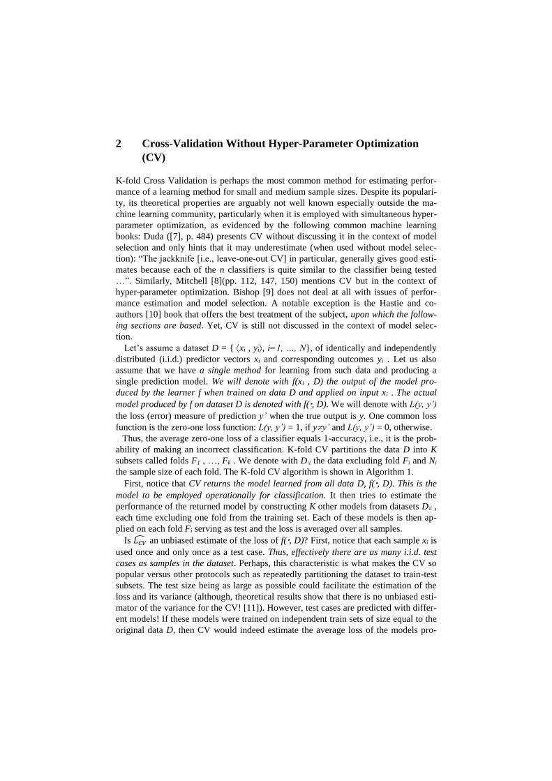
tion. The pseudo-code is shown in Algorithm 2. The symbol f(x, D, 𝑎 ) now denotes
the output of the model learned when using hyper-parameters a on dataset D and ap-
plied on input x. Correspondingly, the symbol f(•, D, 𝑎 ) denotes the model produced
by applying hyper-parameters a on D. The quantity 𝐿𝐶𝑉(𝑎) is now parameterized by
the specific values a and the minimizer of the loss (maximizer of performance) a* is
found. The final model returned is f(•, D, 𝑎∗), i.e. , the models produced by values a*
on all data D. On one hand, we expect CV with model selection (hereafter, CVM) to
underestimate performance because estimations are computed using models trained
on only a subset of the dataset. On the other hand, we expect CVM to overestimate
performance because it returns the maximum performance found after trying several
hyper-parameter values. In Section 7 we examine this behavior empirically and de-
termine (in concordance with [2],[4]) that indeed when sample size is relatively small
and the number of models in the hundreds CVM overestimates performance. Thus, in
these cases other types of estimation protocols are required.
4 The Tibshirani and Tibshirani (TT) Method
The TT method [5] attempts to heuristically and approximately estimate the bias of
the CV error estimation due to model selection and add it to the final estimate. For
Algorithm 2: K-Fold Cross-Validation with Hyper-
Parameter Optimization (Model Selection) CVM(D, 𝒂)
Input: A dataset D = {xi , yi, i=1, …, N}
A set of hyper-parameter value combinations 𝒂 Output: A model M
An estimation of performance (loss) of M
Partition D to K folds Fi
Estimate 𝐿𝐶𝑉(𝑎)̂ for each 𝑎 ∈ 𝒂:
𝑒𝑖(𝑎)̂ =1
𝑁𝑖∑ 𝐿(𝑦𝑗 , 𝑓(𝑥𝑗 , 𝐷\𝑖 , 𝑎)𝑗∈𝐹𝑖
, 𝐿𝐶𝑉(𝑎)̂ =1
𝐾∑ 𝑒𝑖(𝑎)̂𝐾
𝑖=1
Find minimizer 𝑎∗ of 𝐿𝐶𝑉(𝑎)̂ // “best hyper-parameters”
M = f(•, D, 𝑎∗) // the model from all data D with the
best hyper-parameters
𝐿𝐶𝑉𝑀̂ = 𝐿𝐶�̂�(𝑎∗)
Return M, 𝐿𝐶𝑉�̂�
Algorithm 3: TT( D, 𝒂)
Input: A dataset D = {xi , yi, i=1, …, N}
A set of hyper-parameter value combinations 𝒂 Output: A model M
An estimation of performance (loss) of M
Partition D to K folds Fi
Estimate 𝐿𝐶𝑉(𝑎)̂ for each 𝑎 ∈ 𝒂:
𝑒𝑖(𝑎)̂ =1
𝑁𝑖∑ 𝐿(𝑦𝑗 , 𝑓(𝑥𝑗 , 𝐷\𝑖 , 𝑎)𝑗∈𝐹𝑖
, 𝐿𝐶𝑉(𝑎)̂ =1
𝐾∑ 𝑒𝑖(𝑎)̂𝐾
𝑖=1
Find minimizer 𝑎∗ of 𝐿𝐶𝑉(𝑎)̂ // “best hyper-parameters”
Find minimizers 𝑎𝑘 of 𝑒𝑘(𝑎) // the minimizers for each fold
Estimate 𝐵𝑖𝑎�̂� = ∑ ( 𝑒𝑘(𝑎∗) − 𝑒𝑘(𝑎𝑘))𝐾𝑘=1
M = f(•, D, 𝑎∗), i.e,. the model learned on all data D
with the best hyper-parameters
𝐿𝑇𝑇̂ = 𝐿𝐶�̂�(𝑎∗) + 𝐵𝑖𝑎�̂�
Return M, ̂𝐿𝑇𝑇̂
each fold, the bias due to model selection is estimated as 𝑒𝑘(𝑎∗) − 𝑒𝑘(𝑎𝑘) where, as
before, ek is the average loss in fold k, ak is the hyper-parameter values that minimizes
the loss for fold k, and a* the global minimizer over all folds. Notice that, if in all
folds the same values ak provide the best performance, then these will also be selected
globally and hence ak = a* for k=1, …, K. In this case, the bias estimate will be zero.
The justification of this estimate for the bias is in [5]. Notice that CVM and TT return
the same model (assuming data are partitioned into the same folds), the one returned
by f on all data D using the minimizer a* of the CV error; however, the two methods
return a different estimate of the performance of this model. It is also quite important
to notice that TT does not require any additional model training and has minimum
computational overhead.
5 The Nested Cross-Validation Method (NCV)
We could not trace who introduced or coined up first the name Nested Cross-
Validation (NCV) method but the authors have independently discovered it and using
it since 2005 [6],[13],[14]; one early comment hinting of the method is in [15]. A
similar method in a bioinformatics analysis was used as early as 2003 [16]. The main
idea is to consider the model selection as part of the learning procedure f. Thus, f tests
several hyper-parameter values, selects the best using CV, and returns a single model.
NCV cross-validates f to estimate the performance of the average model returned by f
just as normal CV would do with any other learning method taking no hyper-
parameters; it’s just that f now contains an internal CV trying to select the best model.
NCV is a generalization of the Train-Validation-Test protocol where one trains on the
Train set for all hyper-parameter values, selects the ones that provide the best perfor-
mance on Validation, trains on Train+Validation a single model using the best-found
values and estimates its performance on Test. Since Test is used only once by a single
model, performance estimation has no bias due to the model selection process. The
final model is trained on all data using the best found values for a. NCV generalizes
the above protocol to cross-validate every step of this procedure: for each Test, all
folds serve as Validation, and this process is repeated for each fold serving as Test.
The pseudo-code is shown in Algorithm 4. The pseudo-code is similar to CV (Algo-
rithm 1) with CVM (Cross-Validation with Model Selection, Algorithm 2) serving as
the learning function f. Notice, that NCV returns the same final, single model as CV
and TT (assuming the same partition of the data to folds). Again, the difference re-
gards only the estimation of the performance of this model. NCV requires a quadratic
number of models to be trained to the number of folds K (one model is trained for
every possible pair of two folds serving as test and validation respectively) and thus it
is the most computationally expensive protocol out of the three.
6 Stratification of Folds
In CV folds are partitioned randomly which should maintain on average the same
class distribution in each fold. However, in small sample size sizes or highly imbal-

anced class distributions it may happen that some folds contain no samples from one
of the classes (or in general, the class distribution is very different from the original).
In that case, the estimation of performance for that fold will exclude that class. To
avoid this case, “in stratified cross-validation, the folds are stratified so that they con-
tain approximately the same proportions of labels as the original dataset” [4]. Notice
that leave-one-out CV guarantees that each fold will be unstratified since it contains
only one sample which can cause serious estimation problems ([12], p. 151, [4]).
7 Empirical Comparison of Different Protocols
We performed an empirical comparison in order to assess the characteristics of each
data-analysis protocol. Particularly, we focus on three specific aspects of the protocol
performances: bias, variance of the estimation and the effect of stratification.
7.1 The Experimental Set-Up
Original Datasets: Five datasets from different scientific fields were employed for
the experimentations. The computational task for each dataset consists in predicting a
binary outcome on the basis of a set of numerical predictors (binary classification). In
more detail the SPECT [17] dataset contains data from Single Photon Emission
Computed Tomography images collected in both healthy and cardiac patients. Data in
Gamma [18] consist of simulated registrations of high energy gamma particles in an
atmospheric Cherenkov telescope, where each gamma particle can be originated from
the upper atmosphere (background noise) or being a primary gamma particle (signal).
Discriminating biodegradable vs. non-biodegradable molecules on the basis of their
chemical characteristics is the aim of the Biodeg [19] dataset. The Bank [20] dataset
was gathered by direct marketing campaigns (phone calls) of a Portuguese banking
institution for discriminating customers who want to subscribe a term deposit and
those who don’t. Last, CD4vsCD8 [21] contains the phosphorylation levels of 18
intra-cellular proteins as predictors to discriminate naïve CD4+ and CD8+ human
immune system cells. Table 1 summarizes datasets’ characteristics.
Algorithm 4: K-Fold Nested Cross-Validation NCV(D, 𝒂)
Input: A dataset D = {xi , yi, i=1, …, N}
A set of hyper-parameter value combinations 𝒂 Output: A model M
An estimation of performance (loss) of M
Partition D to K folds Fi
M, ~ = CVM(D, 𝒂)
Estimation 𝐿𝑁𝐶�̂�:
𝑒�̂� =1
𝑁𝑖∑ 𝐿(𝑦𝑗 , 𝐶𝑉𝑀(𝑥𝑗 , 𝐷\𝑖))𝑗∈𝐹𝑖
, 𝐿𝐶�̂� =1
𝐾∑ 𝑒�̂�
𝐾𝑖=1
Return M, 𝐿𝑁𝐶�̂�

Table 1. Datasets‘ characteristics. Dpool is a 30% partition from which sub-sampled datasets
are produced. Dhold-out is the remaining 70% of samples from which an estimation of the true
performance is computed.
Dataset Name # Samples # Attributes Classes
ratio |Dpoo1| |Dhold-out| Ref.
SPECT 267 22 3.85 81 186 [17]
Biodeg 1055 41 1.96 317 738 [19]
Gamma 19020 11 1.84 5706 13314 [18]
CD4vsCD8 24126 18 1.13 7238 16888 [21]
Bank 45211 17 7.54 13564 31647 [20]
Sub-Datasets and Hold-out Datasets. Each original dataset D is partitioned into two
separate, stratified parts: Dpool, containing 30% of the total samples, and the hold-out
set Dhold-out, consisting of the remaining samples. Subsequently, for each Dpool 50 sub-
datasets are randomly sampled with replacement for each sample size in the set {20,
40, 60, 80, 100, 500 and 1500}, for a total of 5 7 50 sub-datasets Di, j, k (where i
indexes the original dataset, j the sample size, and k the sub-sampling). For sample
sizes less than 100 we enforce an equal percentage among the two classes, in order to
avoid problems of imbalanced data. Most of the original datasets have been selected
with a relatively large sample size so that each Dhold-out is large enough to allow a very
accurate (low variance) estimation of performance. In addition, the size of Dpool is
also relatively large so that each sub-sampled dataset to be approximately considered
a dataset independently sampled from the data population of the problem. Neverthe-
less, we also include a couple of datasets with smaller sample size.
Bias and Variance of each Protocol: For each of the data analysis protocols CVM,
TT, and NCV both the stratified and the non-stratified versions are applied to each
sub-dataset, in order to select the “best model/hyper-parameter values” and estimate
its performance �̂�. For each sub-dataset, the same split in 𝐾 = 10 folds was em-
ployed for the stratified versions of CVM, TT and NCV, so that the three data-analysis
protocols always select exactly the same model, and differ only in the estimation of
performance. For the NCV, the internal CV loop uses K=9. The bias is computed as
Lhold-out - �̂�. Thus, a positive bias indicates a higher “true” error (i.e., as estimated on
the hold-out set) than the one estimated by the corresponding analysis protocol and
implies the estimation protocol is optimistic. For each protocol, original dataset, and
sample size the mean bias, its variance and its standard deviation over the 50 sub-
samplings are computed and reported in the results’ Tables and Figures below.

Performance Metric: All algorithms are presented using a loss function L computed
for each sample and averaged out for each fold and then over all folds. The zero-one
loss function is typically assumed corresponding to 1-accuracy of the classifier. How-
ever, we prefer to use the Area Under the Receiver’s Operating Characteristic Curve
(AUC) [22] as the metric of choice for binary classification problems. One advantage
is that the AUC does not depend on the prior class distribution. This is necessary in
order to pool together estimations stemming from different datasets. In contrast, the
zero-one loss depends on the class distribution: for a problem with class distribution
of 50-50%, a classifier with accuracy 85% has greatly improved over the baseline of a
trivial classifier predicting the majority class; for a problem of 84-16% class distribu-
tion, a classifier with 85% accuracy has not improved much over the baseline. Unfor-
tunately, the AUC cannot be expressed as a loss function L(y, y’) where y’ is a single
prediction. Nevertheless, all Algorithms 1-4 remain the same if we substitute 𝑒�̂� =
1 − 𝐴𝑈𝐶(𝑓(⋅, 𝐷\𝑖), 𝐹𝑖), i.e., the error in fold i is 1 minus the AUC of the model
learned by f on all data except fold Fi, as estimated on Fi as the test set.
Model Selection: For generating the hyper-parameter vectors in a we employed three
different modelers: the Logistic Regression classifier ([9], p. 205), as implemented in
Fig. 1. Average loss bias for estimation protocols stratified CVM, TT, and NCV that in-
clude model selection. CVM is clearly optimistic and systematically overestimates perfor-
mance for sample sizes less or equal to 100. TT and NCV do not substantially and system-
atically overestimate on average, although results vary with dataset.
Fig. 2. Standard deviation of bias over the 50 sub-samplings. CVM has the smallest
variance but it overestimates performance. TT and NCV exhibit similar stds.

Matlab 2013b, that takes no hyper-parameters; the Decision Tree [23], as implement-
ed also in Matlab 2013b with hyper-parameters MinLeaf and MinParents both within
{1, 2, …, 10, 20, 30, 40, 50}; Support Vector Machines as implemented in the libsvm
software [24] with linear, Gaussian (𝛾 ∈ {0.01, 0.1, 1, 10, 100}) and polynomial (de-
gree 𝑑 ∈ {2,3,4}, 𝛾 ∈ {0.01, 0.1, 1, 10, 100}) kernels, and cost parameter 𝐶 ∈{0.01, 0.1, 1, 10, 100}. When a classifier takes multiple hyper-parameters, all combi-
nations of choices are tried. Overall, 271 hyper-parameter value combinations and
corresponding models are produced each time to select the best.
7.2 Experimental Results
Fig. 1 shows the average loss bias of CVM, TT, and NCV showing that indeed CVM
overestimates performance for small sample sizes (underestimates error) corroborat-
ing the results in [2],[4]. TT and NCV do not substantially and systematically overes-
timate, although results vary with dataset. Table 2 shows the bias averaged over all
datasets, where it is shown that CVM often overestimates the AUC by more than 5
points for small sample sizes. TT seems quite robust with the bias being confined to
less than plus or minus 1,7 AUC points for sample sizes more than 20. We perform a
t-test for the null hypothesis that the bias is zero, which is typically rejected: all meth-
ods usually exhibit some bias whether positive or negative. Nevertheless, in our opin-
ion the bias for TT and NCV is in general acceptable. The non-stratified versions of
the protocols have more bias in general. Fig. 2 shows the standard deviation (std) of
CVM, TT, and NCV. CVM exhibits the smallest std (and thus variance) but in our
opinion it should be avoided since it overestimates performance. Table 3 shows the
averaged std of the bias over all datasets. We apply the O'Brien's modification of
Levene's statistical test [25] with the null hypothesis that the variance of a method is
the same as the corresponding variance for the same sample size as the NCV. NCV
and TT show almost statistically indistinguishable variances. Thus, within the scope
of our experiments and based on the combined analysis of average bias, average
variance, and computational complexity the TT protocol seems to be the method of
choice. The non-stratified versions also exhibit slightly larger variance and again,
stratification seems to have only beneficial effects.
8 Related Work, Discussion and Conclusions
Estimating performance of the final reported model while simultaneously selecting
the best pipeline of algorithms and turning their hyper-parameters is a fundamental
task for any data analyst. Yet, arguably these issues have not been examined in full
depth in the literature. The origins of cross-validation in statistics can be traced back
to the “jackknife” technique of Quenouille [26] in the statistical community.
In machine learning, [4] studied the cross-validation without model selection (the title
of the paper may be confusing) comparing it against the bootstrap and reaching the
important conclusion that (a) CV is preferable to the bootstrap, (b) a value of K=10 is
preferable for the number of folds versus a leave-one-out, and (c) stratification is also

always preferable. In terms of theory, Bengio [11] showed that there exist no unbiased
estimator for the variance of the CV performance estimation, which impact hypothe-
sis testing of performance using the CV.
To the extent of our knowledge the first to study the problem of bias in the context
of model selection in machine learning is [3]. Varma [27] demonstrated the optimism
of the CVM protocol and instead suggests the use of the NCV protocol. Unfortunate-
ly, all their experiments are performed on simulated data only. Tibshirani and Tibshi-
rani [5] introduced the TT protocol but unfortunately they do not compare it against
alternatives and they include only a proof-of-concept experiment on a single dataset.
Thus, the present paper is the first work that compares all three protocols (CVM,
NCV, and TT) on multiple real datasets.
Based on our experiments we found evidence that the TT method is unbiased
(slightly conservative) for sample sizes above 20, has about the same variance as the
NCV (the other conservative alternative), and does not introduce additional computa-
tional overhead. Within the scope of our experiments, we would thus suggest analysts
to employ the TT estimation protocol. In addition, we corroborate the results in [4]
that stratification exhibits smaller estimation variance and we encourage its use.
Table 2. Average Bias over Datasets. P-values produced by a t-test with null hypothesis
the mean bias is zero (P<0,05* , P<0,01**). NS stands for Non-Stratified. CVM
systematically overestimates performance. TT and NCV slightly underestimate
performance for larger sample sizes.
CVM NS-CVM TT NS-TT NCV NS-NCV
20 0,1551** 0,1892** 0,0525** 0,1142** -0,0007 -0,032*
40 0,0891** 0,0993** 0,0085 0,0172* -0,054** -0,1102**
60 0,0749** 0,0825** 0,0045 0,0136* 0,0083 0,0111
80 0,0507** 0,0563** -0,0176** -0,0097 -0,0228** -0,0338**
100 0,0681** 0,0731** -0,0036 0,0079 0,0131* 0,0183**
500 0,0072** 0,0073** -0,025** -0,0261** -0,0054* -0,0055*
1500 -0,0005 0,0002 -0,0139** -0,0136** -0,0034** -0,003*
Table 3. Average bias STDs over Datasets. P-values produced by a test with null
hypothesis that the variances are the same as the corresponding variance of the NCV
protocol (P<0,05* , P<0,01**). NS stands for Non-Stratified. NCV and TT have
indinstinguishable variances and are conservative. CVM has smaller variance but
overestimates performance.
CVM NS-CVM TT NS-TT NCV NS-NCV
20 0,1134** 0,119** 0,1826 0,1989** 0,1616 0,2055**
40 0,0751** 0,0808** 0,1194** 0,1298* 0,1571 0,1784
60 0,0659* 0,0727 0,0916 0,1017 0,0828 0,0936
80 0,0497** 0,0526** 0,0757 0,0804 0,0731 0,0871*
100 0,0651* 0,0697 0,0917 0,0903 0,0826 0,0845
500 0,028 0,0237 0,0341 0,0351 0,0285 0,0308
1500 0,0119 0,014 0,018** 0,0192** 0,0125 0,0143

We would also like to acknowledge the limited scope of our experiments in terms
of the number and type of datasets, the inclusion of other steps into the analysis (such
as variable selection), the inclusion of other procedures for hyper-parameter optimiza-
tion that dynamically decide to consider value combinations, varying the number of
folds K in the protocols, using other performance metrics, experimentation with re-
gression methods and others which form our future work on the subject in order to
obtain definite answers to these research questions.
We also note the concerning issue that the variance of estimation for small sample
sizes is large, again in concordance with the experiments in [2]. The authors in the
latter advocate methods that may be biased but exhibit reduced variance. However,
we believe that CVM is too biased no matter its variance; implicitly the authors in [2]
agree when they declare that model selection should be integrated in the performance
estimation procedure in such a way that test samples are never employed for selecting
the best model. Instead, they suggest as alternatives limiting the extent of the search
of the hyper-parameters or performing model averaging. In our opinion, neither op-
tion is satisfactory for all analysis purposes and more research is required.
9 Acknowledgements
This work was conducted partially in the framework of the BIOSYS research project,
Action KRIPIS, project No MIS-448301 (2013SE01380036) by the Greek General
Secretariat for Research and Technology. It was funded partially by the STATegra
EU FP7 project, No 306000.
10 References
1. Anguita, D., Ghio, A., Oneto, L., Ridella, S.: In-Sample and Out-of-Sample Model
Selection and Error Estimation for Support Vector Machines. IEEE Trans. Neural
Networks Learn. Syst. 23, 1390–1406 (2012).
2. Cawley, G.C., Talbot, N.L.C.: On Over-fitting in Model Selection and Subsequent
Selection Bias in Performance Evaluation. J. Mach. Learn. Res. 11, 2079–2107
(2010).
3. Jensen, D.D., Cohen, P.R.: Multiple comparisons in induction algorithms. Mach.
Learn. 38, 309–338 (2000).
4. Kohavi, R.: A Study of Cross-Validation and Bootstrap for Accuracy Estimation and
Model Selection. International Joint Conference on Artificial Intelligence. pp. 1137–
1143 (1995).
5. Tibshirani, R.J., Tibshirani, R.: A bias correction for the minimum error rate in cross-
validation. Ann. Appl. Stat. 3, 822–829 (2009).
6. Statnikov, A., Aliferis, C.F., Tsamardinos, I., Hardin, D., Levy, S.: A comprehensive
evaluation of multicategory classification methods for microarray gene expression
cancer diagnosis. Bioinformatics. 21, 631–43 (2005).
7. Duda, R.O., Hart, P.E., Stork, D.G.: Pattern Classification (2nd Edition). (2000).
8. Mitchell, T.M.: Machine Learning. (1997).
9. Bishop, C.M.: Pattern Recognition and Machine Learning (Information Science and
Statistics). (2006).

10. Hastie, T., Tibshirani, R., Friedman, J.: The Elements of Statistical Learning.
Elements. 1, 337–387 (2009).
11. Bengio, Y., Grandvalet, Y.: Bias in Estimating the Variance of K-Fold Cross-
Validation. Statistical Modeling and Analysis for Complex Data Problem. pp. 75–95
(2005).
12. Witten, I.H., Frank, E.: Data Mining: Practical Machine Learning Tools and
Techniques, Second Edition (Morgan Kaufmann Series in Data Management
Systems). (2005).
13. Lagani, V., Tsamardinos, I.: Structure-based variable selection for survival data.
Bioinformatics. 26, 1887–1894 (2010).
14. Statnikov, A., Tsamardinos, I., Dosbayev, Y., Aliferis, C.F.: GEMS: a system for
automated cancer diagnosis and biomarker discovery from microarray gene expression
data. Int. J. Med. Inform. 74, 491–503 (2005).
15. Salzberg, S.: On Comparing Classifiers : Pitfalls to Avoid and a Recommended
Approach. Data Min. Knowl. Discov. 328, 317–328 (1997).
16. Iizuka, N., Oka, M., Yamada-Okabe, H., Nishida, M., Maeda, Y., Mori, N., Takao, T.,
Tamesa, T., Tangoku, A., Tabuchi, H., Hamada, K., Nakayama, H., Ishitsuka, H.,
Miyamoto, T., Hirabayashi, A., Uchimura, S., Hamamoto, Y.: Oligonucleotide
microarray for prediction of early intrahepatic recurrence of hepatocellular carcinoma
after curative resection. Lancet. 361, 923–9 (2003).
17. Kurgan, L.A., Cios, K.J., Tadeusiewicz, R., Ogiela, M., Goodenday, L.S.: Knowledge
discovery approach to automated cardiac SPECT diagnosis. Artif. Intell. Med. 23,
149–69 (2001).
18. Bock, R.K., Chilingarian, A., Gaug, M., Hakl, F., Hengstebeck, T., Jiřina, M.,
Klaschka, J., Kotrč, E., Savický, P., Towers, S., Vaiciulis, A., Wittek, W.: Methods for
multidimensional event classification: a case study using images from a Cherenkov
gamma-ray telescope. Nucl. Instruments Methods Phys. Res. Sect. A Accel.
Spectrometers, Detect. Assoc. Equip. 516, 511–528 (2004).
19. Mansouri, K., Ringsted, T., Ballabio, D., Todeschini, R., Consonni, V.: Quantitative
structure-activity relationship models for ready biodegradability of chemicals. J.
Chem. Inf. Model. 53, 867–78 (2013).
20. Moro, S., Laureano, R.M.S.: Using Data Mining for Bank Direct Marketing: An
application of the CRISP-DM methodology. Eur. Simul. Model. Conf. 117–121
(2011).
21. Bendall, S.C., Simonds, E.F., Qiu, P., Amir, E.D., Krutzik, P.O., Finck, R., Bruggner,
R. V, Melamed, R., Trejo, A., Ornatsky, O.I., Balderas, R.S., Plevritis, S.K., Sachs, K.,
Pe’er, D., Tanner, S.D., Nolan, G.P.: Single-cell mass cytometry of differential
immune and drug responses across a human hematopoietic continuum. Science. 332,
687–96 (2011).
22. Fawcett, T.: An introduction to ROC analysis, (2006).
23. Coppersmith, D., Hong, S.J., Hosking, J.R.M.: Partitioning Nominal Attributes in
Decision Trees. Data Min. Knowl. Discov. 3, 197–217 (1999).
24. Chang, C.-C., Lin, C.-J.: LIBSVM: a library for support vector machines. ACM Trans.
Intell. Syst. …. 2, 1–39 (2011).
25. O’brien, R.G.: A General ANOVA Method for Robust Tests of Additive Models for
Variances. J. Am. Stat. Assoc. 74, 877–880 (1979).
26. Quenouille, M.H.: Approximate tests of correlation in time-series 3, (1949).
27. Varma, S., Simon, R.: Bias in error estimation when using cross-validation for model
selection. BMC Bioinformatics. 7, 91 (2006).
Related Documents