Performance-Based Design of Distributed Real-Time Systems

Performance-Based Design of Distributed Real-Time Systems �Dong-In Kang, Richard GerberInstitute for Advanced Computer StudiesDepartment of Computer ScienceUniversity of MarylandCollege Park, MD 20742fdikang, [email protected] Manas SaksenaDept. of Computer ScienceConcordia UniversityMontreal Quebec H3G [email protected] paper presents a design method for distributedsystems with statistical, end-to-end real-time con-straints, and with underlying stochastic resource re-quirements. A system is modeled as a set of chains,where each chain is a distributed pipeline of tasks, anda task can represent any activity requiring nonzeroload from some CPU or network resource. Every chainhas two end-to-end performance requirements: Its de-lay constraint denotes the maximum amount time acomputation can take to ow through the pipeline,from input to output. A chain's quality constraintmandates a minimum allowable success rate for out-puts that meet their delay constraints. Our designmethod solves this problem by deriving (1) a �xed pro-portion of resource load to give each task; and (2) adeterministic processing rate for every chain, in whichthe objective is to optimize the output success rate (asdetermined by an analytical approximation).We demonstrate our technique on an example sys-tem, and compare the estimated success rates withthose derived via simulated on-line behavior.1 IntroductionScheduling analysis can often be a valuable tool inthe design of a hard real-time system. Traditionally,this kind of system is characterized by two key cri-teria. First, all execution times and communicationdelays can be deterministically bounded; the designerassumes that these worst-case bounds may be su�eredeach time a task is run, or whenever a packet is sent.Second, all real-time constraints are known ahead of�This research is supported in part by ONR grant N00014-94-10228, NSF Young Investigator Award CCR-9357850, ARLCooperative Agreement DAAL01-96-2-0002 and NSERC Oper-ating Grant OGPO170345.

time, and are part of the system's requirements { orderive from them in some logical way. Such constraintsmight include an individual task's period, a message'sdeadline, or perhaps the rate at which a network driveris run. Given this type of system, real-time schedulinganalysis can often be used to predict (and then ensure)that the performance objectives will be met.Of course, while hard real-time applications do exist(e.g., reactor shutdown systems come to mind), manysystems cannot be designed like this. First, while onecould theoretically bound all execution times and net-work delays, these bounds would never be tight. Con-temporary systems make this almost impossible, byincluding features like superscalar pipelining, hierar-chies of cache memory, etc. { not to mention the non-determinism inherent in almost any network. Asidefrom these physical limitations, since a program's ac-tual execution time is almost always data-dependent,its worst-case time may be several orders of magni-tude greater than the mean. Hence, if one incorpo-rates worst-case costs in a design, the result will be anextremely under-utilized system.Second, most real-time constraints are not inher-ently part of the system's end-to-end requirements;rather, task and message constraints are artifacts ofthe design itself, and there is rarely an intrinsic needto meet each and every artifact deadline. For exam-ple, consider a video-conferencing system. It shouldbe able to capture, process, transmit, receive, process,and display the data at some mean frame-rate, albeitwith permissible deviations for jitter. Or consider areal-time control system, which might involve sam-pling, computation, and actuation; thus the control-loop is typically implemented as a periodic task with adeadline. In both these cases, real-time performancerequirements are usually intended to enforce an ac-ceptable level of quality, and do not hinge on the sys-tem meeting all of its artifact's deadlines. In otherwords, while hard real-time scheduling theory provides

a su�cient way to build such systems, it is not strictlynecessary, and is probably not the most cost-e�ectivedesign framework.In this paper we explore an alternative approach, byusing statistical guarantees to generate cost-e�ectivesystem designs. We model a real-time system as a setof task chains, with each task representing some activ-ity requiring a speci�c CPU or network link. For ex-ample, a chain may correspond to the data path froma camera to a display in a video conferencing system,or may re ect a servo-loop in a distributed real-timecontrol system. The chain's real-time performance re-quirements are speci�ed in terms of (i) a maximumac-ceptable propagation delay from input to output, and(ii) a minimumacceptable average throughput. In de-signing the system, we treat the �rst requirement asa hard requirement, that is, any end-to-end compu-tation that takes longer than the maximum delay istreated a failure, and does not contribute to the over-all throughput. In contrast, the second requirement isviewed in a statistical sense, and we design a system toexceed, on average, its minimal acceptable rate. Weassume that a task's cost (i.e., execution time for aprogram, or delay for a network link) can be speci�edwith any arbitrary (discrete) probability distributionfunction.Problem and Solution Strategy. Given a set oftask chains, each with its own real-time performancerequirements, our objective is to design a system whichwill meet the requirements for all of the chains. Oursolution uses several techniques to make the problemtractable:� We assume a static partitioning of the system re-sources; in other words, a task has already beenallocated to a speci�c resource.� A task's load requirements are expressed stochas-tically, in terms of a discrete probability distri-bution function (or PDF), whose random vari-able characterizes the resource time needed forone execution instance of the task. All successiveinstances are modeled to be independent of eachother.While our objective is to achieve an overall, statisti-cal level of real-time performance, we can still use thetools provided by hard real-time scheduling to helpsolve this problem. Our method involves (1) assign-ing a �xed period to a chain, so that (if possible) thechain's tasks are invoked at the periodic boundaries;and (2) assigning to each task a �xed proportion ofits resource's load. Then, using the techniques pro-vided by real-time CPU and network scheduling, wecan guarantee that during any period, a task will get

at least its designated share of the resource's time.When that share fails to be su�cient for the task to�nish executing, it runs over into the next period {and gets that period's share, etc. Given this model,the design problem may be viewed as the followinginterrelated sub-problems:(1) Given a set of chains, how should the CPU andnetwork load be partitioned among the tasks, sothat every chain's performance requirements aremet?(2) Given a load-assignment to the tasks in a chain,what is the optimal period to execute the chainsuch that the e�ective throughput is maximized?In this paper we present algorithms to solve theseproblems. The algorithm for problem (1) uses aheuristic to compare the relative needs of tasks fromdi�erent chains competing for the same resources. Thealgorithm for problem (2) makes use of connectingMarkov chains, to estimate the e�ective throughputof a given chain. Since the analysis is approximate,we validate the solution generated using a simulationmodel.Related Work. Like much of the work in real-timesystems, our results extend from preemptive, unipro-cessor scheduling analysis. There are many old andnew solutions to this problem (e.g., [11, 1, 7, 10]);moreover, these methods come equipped o�ine, anal-ysis tests, which determine a priori whether the un-derlying system is schedulable. Many of these testsare load-oriented su�ciency conditions { they predictthat the tasks will always meet their deadlines, pro-vided that the system utilization does not exceed acertain pre-de�ned threshold.The classical model has been generalized to a largedegree, so that there now exist analogous results fordistributed systems, network protocols, etc. For ex-ample, the model has been applied to distributedhard real-time systems in the following straightfor-ward manner (e.g., see [14, 20]): each network con-nection is abstracted as a real-time task (sharing anetwork resource), and the scheduling analysis incor-porates worst-case blocking times potentially su�eredwhen high-priority packets have to wait for transmis-sion of lower-priority packets. Then, to some extent,the resulting global scheduling problem can be solvedas a set of interrelated local resource-scheduling prob-lems.In our previous work [4] we relaxed the preconditionthat period and deadline parameters are always knownahead of time. Rather, we used the system's end-to-end delay and jitter requirements to automatically de-rive each task's constraints; these, in turn, ensure that

the end-to-end requirements will be met on a unipro-cessor system. This idea was also used recently in [15],where individual task constraints are derived from aset of control laws { with the objective being to opti-mize the system's performance index while satisfyingschedulability. A similar approach has been used for\soft" transactions in distributed systems [8], whereeach transaction's deadline is partitioned between thesystem's resources.As for modeling stochastic execution times, somerecent results deal with uniprocessor systems, andwhere the artifact, real-time constraints are consid-ered part of the system's requirements. For example,in [18] task completion time bounds are found for thecase in which costs can vary within some range, andwhere arrivals can be sporadic. And in [19], schedulinganalysis is extended to consider probabilistic executiontimes on uniprocessor systems. This is done by givinga nominal \hard" amount of execution time to eachtask instance, under the assumption that the task willusually complete within this time. But if the nominaltime is exceeded, the excess requirement is treated likea sporadic arrival (via a method similar to that usedin [9]).To our knowledge, however, ours is the �rst tech-nique that achieves statistical real-time performancein a distributed system, by using end-to-end require-ments to assign both periods and the execution timebudgets. In this light, our method should be viewedless as a scheduling tool (it is not one), and more as anapproach to the problem of real-time systems design.To accomplish this goal, we assume an underlyingruntime system that is capable of the following: (1) de-creasing a task's completion time by proportionatelyincreasing its resource share; (2) enforcing, for eachresource, the proportional shares allocated for everytask, up to some minimum, pre-de�ned window size;and (3) within these constraints, isolating a task'sreal-time behavior from the other activities sharingits resource. In this regard, we are building on manyrecent results that have been developed for provid-ing OS-level reservation guarantees, and for fair-sharequeueing in network protocols.In particular, we assume a network model in whichper-connection real-time performance guarantees canbe provided, assuming that a certain proportion ofbandwidth has been allocated to each connection.Many policies have recently proposed to accommodatethis, including the \Virtual Clock Method" [24], \Fair-Share Queueing" [2], \Generalized Processor Sharing"(or GPS) [13], and \Rate Controlled Static PriorityQueueing" (or RCSP) [22]. These models have alsobeen extended to derive statistical guarantees; in par-ticular, within the framework of RCSP (in [23]), andfor GPS (in [25]). Related results for real-time traf-

�c sources can be found in [3] (using a policy like\Virtual Clock" [24]), and in [21] (using a modi-�ed FCFS method, with a variety of tra�c distribu-tions). In [6], statistical service quality is achievedvia proportional-share queueing, in conjunction withserver-guided backo�; i.e, servers dynamically adjusttheir rates to help utilize the available bandwidth, andto avoid network congestion.Many of the proportional-sharing techniques willsu�ce for our purposes, since all we require are (1) themutual independence of all sessions running througha switch, given proportional bandwidth allocations foreach; and (2) delay distributions for all single-hop con-nections. With this abstraction, we are able to modela single-hop connection like a real-time task, whichshares a network resource (as opposed to a CPU).We also rely on a similar model at the CPUlevel, and there have been many policies suggested toachieve this end. (In fact, rate-monotonic and EDFscheduling can be considered two such policies.) More-over, several recent schemes have been proposed toguarantee processor capacity shares for the system'sreal-time tasks, and to simultaneously isolate themfrom overruns caused by other tasks in the system. Forexample, Mercer et al. [12] proposed a processor capac-ity reservation mechanism to achieve this, a methodwhich enforces each task's reserved share within itsreservation period, under micro-kernel control. Also,Shin et al. [16] proposed a reservation-based algorithmto guarantee the performance of periodic real-timetasks, and also improve the schedulability of aperiodictasks.Recently, many of the rate-based disciplines devel-oped for network queueing have sprouted analoguesfor CPU scheduling. In particular, Goyal et al. [5]proposed a scheme which allows for hierarchical parti-tioning of CPU load, so multiple classes of tasks (e.g.,hard and soft real-time applications) can coexist in thesame system. Also, Stoica et al. [17] developed a pro-portional share scheduling strategy, which multiplexesavailable CPU load according to relative weights of theconstituent tasks. Like the abovementioned schemesused for network queueing, this method maps a task'sreal-time state-changes onto a virtual time-line, andthen schedules the tasks via a virtual clock.2 Model and Solution OverviewAs stated above, we model a system as set ofindependent, pipelined task chains, with every taskmapped to a designated CPU or network resource.The chain abstraction can, for example, capture theessential data path structure of a video conferencingsystem, or a distributed process control loop. For-

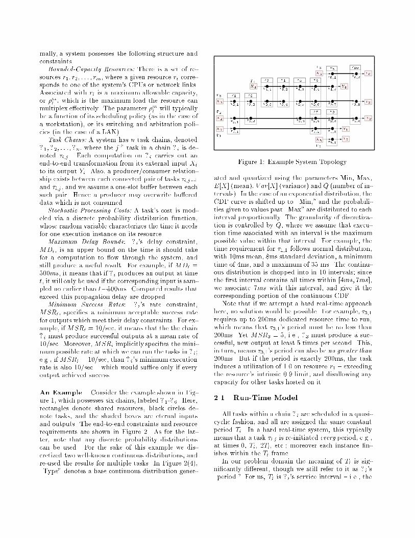
mally, a system possesses the following structure andconstraints.Bounded-Capacity Resources: There is a set of re-sources r1; r2; : : : ; rm, where a given resource ri corre-sponds to one of the system's CPUs or network links.Associated with ri is a maximum allowable capacity,or �mi , which is the maximum load the resource canmultiplex e�ectively. The parameter �mi will typicallybe a function of its scheduling policy (as in the case ofa workstation), or its switching and arbitration poli-cies (in the case of a LAN).Task Chains: A system has n task chains, denoted�1;�2; : : : ;�n, where the jth task in a chain �i is de-noted �i;j . Each computation on �i carries out anend-to-end transformation from its external input Xito its output Yi. Also, a producer/consumer relation-ship exists between each connected pair of tasks �i;j�1and �i;j, and we assume a one-slot bu�er between eachsuch pair. Hence a producer may overwrite bu�ereddata which is not consumed.Stochastic Processing Costs: A task's cost is mod-eled via a discrete probability distribution function,whose random variable characterizes the time it needsfor one execution instance on its resource.Maximum Delay Bounds: �i's delay constraint,MDi, is an upper bound on the time it should takefor a computation to ow through the system, andstill produce a useful result. For example, if MDi =500ms, it means that if �i produces an output at timet, it will only be used if the corresponding input is sam-pled no earlier than t�500ms. Computed results thatexceed this propagation delay are dropped.Minimum Success Rates: �i's rate constraint,MSRi, speci�es a minimum acceptable success ratefor outputs which meet their delay constraints. For ex-ample, if MSRi = 10=sec, it means that the the chain�i must produce successful outputs at a mean rate of10=sec. Moreover,MSRi implicitly speci�es the mini-mum possible rate at which we can run the tasks in �i;e.g., if MSRi = 10=sec, than �i's minimum executionrate is also 10=sec { which would su�ce only if everyoutput achieved success.An Example. Consider the example shown in Fig-ure 1, which possesses six chains, labeled �1-�6. Here,rectangles denote shared resources, black circles de-note tasks, and the shaded boxes are eternal inputsand outputs. The end-to-end constraints and resourcerequirements are shown in Figure 2. As for the lat-ter, note that any discrete probability distributionscan be used. For the sake of this example we dis-cretized two well-known continuous distributions, andre-used the results for multiple tasks. In Figure 2(4),\Type" denotes a base continuous distribution gener-

Y2X1X2X3 X4 r3 Y1Y5X5�2;4�1;2 �2;5�1;3�5;1 �2;6 Y3�3;6 �3;8Y4�4;4 �4;5X6 Y6r5 r6r7 r8 r10r9r2 r4r1�1;1�2;1�3;1 �2;2�3;2 �4;1�3;3 �4;2�3;4 �4;3�3;5 �3;7�2;3 �6;1 �6;2�3 �5�4�2�1 �6Figure 1: Example System Topology.ated and quantized using the parameters Min, Max,E[X] (mean), V ar[X] (variance) and Q (number of in-tervals). In the case of an exponential distribution, theCDF curve is shifted up to \Min," and the probabili-ties given to values past \Max" are distributed to eachinterval proportionally. The granularity of discretiza-tion is controlled by Q, where we assume that execu-tion time associated with an interval is the maximumpossible value within that interval. For example, thetime requirement for �1;1 follows normal distribution,with 10ms mean, 8ms standard deviation, a minimumtime of 4ms, and a maximum of 35 ms. The continu-ous distribution is chopped into in 10 intervals; sincethe �rst interval contains all times within [4ms; 7ms],we associate 7ms with this interval, and give it thecorresponding portion of the continuous CDF.Note that if we attempt a hard real-time approachhere, no solution would be possible. For example, �3;1requires up to 200ms dedicated resource time to run,which means that �3;1's period must be no less than200ms. Yet MSR3 = 5, i.e., �3 must produce a suc-cessful, new output at least 5 times per second. This,in turn, means �3;1's period can also be no greater than200ms. But if the period is exactly 200ms, the taskinduces a utilization of 1.0 on resource r1 { exceedingthe resource's intrinsic 0.9 limit, and disallowing anycapacity for other tasks hosted on it.2.1 Run-Time ModelAll tasks within a chain �i are scheduled in a quasi-cyclic fashion, and all are assigned the same constantperiod Ti. In a hard real-time system, this typicallymeans that a task �i;j is re-initiated every period, e.g.,at times 0, Ti, 2Ti, etc.; moreover each instance �n-ishes within the Ti frame.In our problem domain the meaning of Ti is sig-ni�cantly di�erent, though we still refer to it as �i's\period." For us, Ti is �i's service interval { i.e., the

1. Maximum Delay Constraints (ms):MD1 = 240 , MD2 = 1000, MD3 = 1000MD4 = 700 , MD5 = 100, MD6 = 3002. Minimum Success Rates (per second):MSR1 = 10, MSR2 = 5 , MSR3 = 5MSR4 = 5 , MSR5 = 5, MSR6 = 53. Resource Time PDFs: (ms)Type E[X] V ar[X] [Min,Max] Q TasksNormal 10 64 [4,35] 10 �1;1; �3;2; �3;5; �4;1; �6;1Normal 20 100 [10,50] 20 �1;3; �2;3; �3;6; �3;8; �4;2Exp 10 [0,100] 30 �2;1; �3;4; �3;7; �4;3; �5;1Exp 20 [0, 200] 50 �2;4; �2;6; �3;1; �4;5; �6;2Normal 8 144 [2,48] 20 �1;2; �2;2; �2;5; �3;3; �4;44. Maximum Resource Utilizations:�m1 �m2 �m3 �m4 �m5 �m6 �m7 �m8 �m9 �m100.9 0.7 0.9 0.6 0.9 0.7 0.7 0.8 0.9 0.9Figure 2: Chain Constraints and Task PDF's.time quantum at which �i's load guarantees are main-tained by each of its constituent resources.Our design algorithm assigns each task �i;j a pro-portion of its resource's capacity, which we denote asui;j. Given this assignment, �i;j's runtime behaviorcan be described as follows:(1) Within every Ti interval, the runtime systemensures that �i;j can use up to ui;j of its resource's ca-pacity. This is policed by assigning �i;j an execution-time budget Ei;j = bui;j�Tic; that is, Ei;j is an upperbound on the amount of resource time provided withineach Ti frame, truncated to discrete units. (We as-sume that the system cannot keep track of arbitrarily�ne granularities of time.)(2) A particular execution instance of �i;j may re-quire multiple periods to complete, with Ei;j of itsrunning time expended in each period.(3) A new instance of �i;j will be started within aperiod if no previous instance of �i;j is still running,and if �i;j 's input bu�er contains new data that hasnot already exceeded MDi. This is policed by a time-stamp mechanism, put on the computation when itsinput is sampled.Due to a chain's pipeline structure, note that ifthere are ni tasks in �i, then we must have thatMDi � ni � Ti, since data has to ow through allni elements to produce a computation.2.2 Solution OverviewThe design process works by (1) partitioning theCPU and network capacity between the tasks; (2) se-lecting each chain's period to optimize its success rate;and (3) checking the solution via simulation, to ver-

ify the integrity of the approximations used, and toensure that each chain's output pro�le is su�cientlysmooth (i.e., not bursty).The partitioning algorithm processes each chain �iand �nds a load assignment vector for it, denoted ui.This vector represents the minimal resource load su�-cient for �i to meet its performance objectives, wherean element ui;j in ui contains the load allocated to�i;j on its resource. Now, given a load assignment for�i, we attempt to �nd a period Ti which achieves �i'ssuccess rate. This computation is done approximately:For a given period Ti, a success rate estimate is derivedby (1) treating all of �i's outputs uniformally, whichyields an i.i.d. \success probability" �i for all outputs;and (2) then simplymultiplying �i� 1Ti to approximatethe chain's current success rate, SRi. If SRi is lowerthan the MSRi requirement, the load assignment vec-tor is increased, and so on. Finally, if su�cient loadis found for all chains, the resulting system is simu-lated to ensure that the approximations were sound.At this point, excess resource capacity can be givento any chain, with the hope of improving its overallsuccess rate.3 Throughput AnalysisIn this section we describe how we approximate �i'ssuccess rate, SRi, given a particular period Ti andutilization assignment ui. Then in Section 4, we showhow we make use of this technique to help search forcandidate instantiations of Ti and ui.We carry out our analysis using a discrete-timemodel, in which the time units are in terms of chainperiods; i.e., our discrete domain f0; 1; 2; : : :g corre-sponds to the real times f0; Ti; 2Ti; : : :g. Not only doesthis reduction make the analysis more tractable, it alsocorresponds to our stipulation that tasks can only beinitiated at period boundaries. Moreover, since theunderlying system may schedule a task execution atany time within a Ti frame, we have to assume thatits input data may be read as early as the beginningof a frame, and output as late as the end of a frame.And with one exception, a chain's states of interest dooccur at its period boundaries. That exception is inevaluating a computation's aggregate delay { which,in our discrete time domain, we treat as bMDiTi c. Hencethe fractional part of the last period is ignored, lead-ing to a tighter notion of success (and consequentlyerring on the side conservatism).Theoretically, we could model a computation's de-lay by constructing a stochastic process for the chainas a whole { and solving it for all possible delay prob-abilities. But this would probably be a futile venture,even smaller chains; after all, such a model would have

to simultaneously keep track of each task's local be-havior. And since a chain may hold as few as 0 on-going computations, and as many as one computationper task, it's easy to see how the state-space wouldquickly explode. Instead, we go about constructing amodel in a compositional (albeit inexact) manner, byprocessing each task locally, and using the results forits successors.Now consider the following diagram,which portraysthe ow of a computation at a single task:agei;j�1 Bi;j �i;j�i;j�1 i;j agei;jThe variable agei;j charts a computation's total ac-cumulated time, from entering �i's head, to leaving�i;j. The task reads an incoming input's time-stampas its �rst action; if it exceeds the chain's maximumallowable delay, the input is dropped at that point.Now, there are two types of delay that �i;j can addto agei;j : (1) blocking time, or the time during whichan output from �i;j�1 is blocked in �i;j 's input bu�er;and (2) processing time, i.e., the number of periods�i;j actually needs to perform its computation or datatransfer.A computation su�ers blocking time whenever itsresult arrives from �i;j�1, but �i;j is still un�nishedwith some previous sample. We use the random vari-able Bi;j to describe a tagged data's blocking time attask �i;j.As for processing time, let ti;j be a random variablewhose values are generated via �i;j's execution timePDF. Then, letting i;j be the corresponding randomvariable expressing �i;j's execution time in units of pe-riods, we have that i;j = d ti;jEi;j e.Given this model, and assuming data is alwaysready at the chain's head, agei;j can be calculatedvia the following recurrence relation:agei;1 = i;1agei;j = agei;j�1 +Bi;j + i;jFor j > 1, we approximate the agei;j distribution byassuming the three variables to be independent, i.e.,P [agei;j = k] =Xk1+k2+k3=kP [agei;j�1 = k1]� P [Bi;j = k2]� P [i;j = k3]We also require an approximation of �i;j 's inter-output distribution, �Outi;j, which measures time be-

2 3451 0Figure 3: Chain Xi;j(t), max(i;j) = 6.tween two successive outputs produced by the task.Note that �i;j's success probability, �i;j, will then be1E[�Outi;j ] , i.e., the probability that a (non-stale) out-put is produced during a random period. For the headtask �i;1, we trivially have thatP [�Outi;1 = t] = P [i;1 = t]and that �i;1 is 1E[i;1] . Since �i;1 can retrieve freshinput whenever it is ready (and hence it incurs noblocking time), �i;1 can execute a new phase wheneverit �nishes with the previous phase.Blocking Time Analysis. To help analyze Bi;j , weset up a stochastic process, Xi;j(t), which describesrandom states of �i;j . Speci�cally, we are interestedin capturing (1) �i;j's remaining execution time untilthe next task instance; an (2) whether an input is tobe processed or dropped.Xi;j(t)'s transitions can be described using a sim-ple Markov Chain, as shown in Figure 3 (where themaximum execution time is 6Ti.) The transitions areevent-based, i.e., they are triggered by new inputsfrom �i;j�1. On the other hand, states measure theremaining time left in a current execution, if there isany. When the process moves from state k to l, itmeans that (1) a new input is received; and (2) it willinduce blocking time of l periodic units.For the sake of our analysis, we distinguish betweenthree di�erent outcomes which can occur when statek moves to state l. Here we di as the end-to-end delaybound in periodic units, or di = bMDiTi c.(1) Dropping, de�ned by P d[k ! l]: The task is cur-rently executing, and there is already another inputqueued up in its bu�er { which was calculated to in-duce a blocking-time of k. The new input will over-write it, and induce l blocking-time periods.P d[k ! l] = P [�Outi;j�1 = k � l] (k > l � 0)

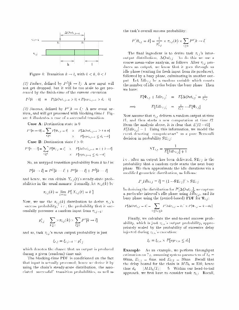
�i;j�1�i;j kt1 t2 l�Outi;j�1Figure 4: Transition k! l, with 0 < k, 0 < l.(2) Failure, de�ned by P f [k ! l]: A new input willnot get dropped, but it will be too stale to get pro-cessed by the �nish-time of the current execution.P f [k ! 0] = P [�Outi;j�1 > k]� P [agei;j�1 > di + k](3) Success, de�ned by P s[k ! l]: A new event ar-rives, and will get processed with blocking time l. Fig-ure 4 illustrates a case of a successful transition.Case A: Destination state is 0.P s[k! 0] =Xt�0 P [i;j = t] � P [�Outi;j�1 � t+ k]� P [agei;j�1 � di � k]Case B: Destination state l > 0:P s[k ! l] =Xt�0 P [i;j = t] � P [�Outi;j�1 = t+ k � l]� P [agei;j�1 � di � k]So, an untyped transition probability from k to l is:P [k! l] = P f [k! l] + P s[k! l] + P d[k! l]and hence, we can obtain Xi;j(t)'s steady-state prob-abilities in the usual manner. Formally, let �i;j(k) be�i;j(k) = limt!1P [Xi;j(t) = k ]Now, we use the �i;j(k) distribution to derive �i;j's\success probability," i.e., the probability that it suc-cessfully processes a random input from �i;j�1:psi;j =Xk�0��i;j(k)�Xl�0 P s[k! l]and so, task �i;j's mean output probability is just�i;j = �i;j�1 � psi;jwhich denotes the chance that an output is producedduring a given (random) time unit.The blocking-time PDF is conditioned on the factthat input is actually processed; hence we derive it byusing the chain's steady-state distribution, the asso-ciated \successful" transition probabilities, as well as

the task's overall success probability:P [Bi;j = k] = 1psi;j � �i;j(k) �Xl�0 P s[k! l]The �nal ingredient is to derive task �i;j's inter-output distribution, �Outi;j. To do this we use acoarse mean-value analysis, as follows. After �i;j pro-duces an output, we know that it goes through anidle phase (waiting for fresh input from its producer),followed by a busy phase, culminating in another out-put. Let Idlei;j be a random variable which countsthe number of idle cycles before the busy phase. Thenwe have: E[i;j + Idlei;j] = E[�Outi;j] = 1�i;j=) E[Idlei;j] = 1�i;j �E[i;j]Now assume that �i;j delivers a random output at timet1, and then starts a new computation at time t2.From the analysis above, it is clear that E[t2� t1] =E[Idlei;j] + 1. Using this information, we model theevent denoting \compute-start" as a pure Bernoullidecision in probability STi;j:STi;j = 1E[Idlei;j ] + 1i.e., after an output has been delivered, STi;j is theprobability that a random cycle starts the next busyphase. We then approximate the idle durations via amodi�ed geometric distribution, as follows:P [Idlei;j = l] = (1� STi;j)l � STi;jIn deriving the distribution for P [�Outi;j], we capturea particular interval's idle phase using Idlei;j, and itsbusy phase using the (period-based) PDF for i;j :P [�Outi;j = k] = X0�k1�kP [Idlei;j = k1]� P [i;j = k � k1 ]Finally, we calculate the end-to-end success prob-ability, which is just �i;n's output probability, appro-priately scaled by the probability of excessive delayinjected during �i;n's execution:�i = �i;n � P [agei;n � di]Example. As an example, we perform throughputestimation on �6, assuming system parameters of T6 =60ms, E6;1 = 6ms, and E6;2 = 30ms. Recall thatthe delay bound for the chain is MD6 = 300; hencethus d6 = bMD6=T6c = 5. Within our head-to-tailapproach, we �rst have to consider task �6;1. Recall,

however, that the distributions for both age6;1 and�Out6;1 follow that for 6;1; moreover, we have that�6;1 = 1E[6;1] = 0:3291:Next we consider the second (and last) task �6;2.The following tables show the PDFs for 6;2, for theMarkov Chain's steady states, the blocking times, andfor age6;2.k P [6;2 ] �6;2(0) P [B6;2 ] P [age6;2 ]0 0:0 0:975 0:980 0:01 0:7543 0:019 0:017 0:02 0:1968 0:0045 0:002 0:03 0:03751 0:0009 0:00009 0:26584 0:0098 0:0002 0:0 0:34005 0:0019 0:00003 0:0 0:24466 0:0005 0:000001 0:0 0:11537 0:00008 0:0 0:0 0:02698 0:0 0:0 0:0 5:7� 10�39 0:0 0:0 0:0 1:3� 10�310 0:0 0:0 0:0 2:7� 10�411 0:0 0:0 0:0 5:3� 10�512 0:0 0:0 0:0 5:8� 10�6Again, the success probability is derived as follows:ps6;2 = 0:9804�6;2 = �6;1 � ps6;2 = 0:3228P [age6;2 � d6] = 0:850�6 = �6;2 � P [age6;2 � d6] = 0:2745And hence, SR6 = 0:2745� 100060 = 4:5744 System Design ProcessWe now revisit the \high-level" problem of deter-mining the system's parameters, with the objective ofsatisfying each chain's performance requirements. Asstated in the introduction, the design problem may beviewed as two inter-related sub-problems:(1) Load Assignment. Given a set of chains, howshould the CPU and network load be partitionedamong the set of tasks, so that the performancerequirements are met?(2) Rate Assignment. Given a load-assignment tothe tasks in the chain, what is the optimal pe-riod to execute the chain such that the e�ectivethroughput is maximized?Our solution uses separate heuristics for each of thesesub-problems. In particular, the top-level \Load As-signment" algorithm works on a chain-by-chain basis,iteratively adjusting the proportional load allocatedto each of the chain's tasks. In doing this, it makesuse of a \Rate Assignment" subroutine, which deter-mines a suitable processing rate for a chain, under thegiven load assignment { and computes the correspond-ing success rate.

Algorithm 4.1 Load-Assignment AlgorithmOutput :fui : 1 � i � ng, where each ui is the utilization vector for �ifTi : 1 � i � ng, where each Ti is the period of �ifSRi : 1 � i � ng, where each SRi is the success ratefor �i at period TiAlgorithm :(1) foreach (resource rk)(2) �k �mk(3) foreach (�i : 1 � i � n)f(4) Ti d 1000MSRi e(5) foreach (�i;j in �i with rk = resource(�i;j)f(6) ui;j E[ti;j]Ti(7) �k �k � ui;jg(8) (SRi; Ti) Evaluate Success Rate(�i; Ti;ui)g(9) S f�i : 1 � i � n;SRi < MSRig(10) while (S 6= ;)f(11) Find the �i;j in �i 2 S,with rk = resource(�i;j) that maximizes(12) wi;j MSRi�SRiMSRi � �kui;j(13) if(�k < �)(14) return Failure(15) ui;j ui;j + �(16) �k �k � �(17) (SRi; Ti) Evaluate Success Rate(�i, Ti,ui)(18) if ( SRi � MSRi )(19) S S � f�igg(20) return Feasible SolutionFigure 5: Top-Level Load-Assignment Algorithm.Load AssignmentAlgorithm.The load assignmentalgorithm is presented in Figure 5. Consider a partic-ular chain �i, and note that Ti (expressed in millisec-onds) is initialized to the highest period that couldpotentially achieve the desired success rate MSRi(step (4)). Also note that task �i;j's resource shareui;j is initialized to accommodate its mean executiontime E[ti;j], and that its host resource's capacity isdepleted by the same amount (steps (6)-(7)). (Notethat the system could only be solved with these initialparameters if all execution times were constant.)The algorithm works by iteratively re�ning theload-assignment vectors (the ui's), until a feasible so-lution is found. The entire algorithm terminates whenthe success rate for all chains meet their performancerequirements { or when it discovers that no solutionis possible. The load assignment problem is thus asearch over the space of utilization vectors.In order to control the complexity of the search,two restrictions are made on the search procedure: (1)there is no backtracking, and (2) the load assignmentof a task is never reduced. Hence, since the entiresolution space is not searched, the algorithm is an ap-

Algorithm 4.2 Evaluate Success Rate (�i, Ti,ui)Input :Chain �iUtilization vector ui of �iPeriod Ti for �iOutput :Success Rate for �i, and its associated period TiAlgorithm :(1) SRi get success rate(�i,Ti,ui)(2) for (t Ti � 1; t > 0 ; t t� 1)(3) if ((MDi mod t) < (�� t)) f(4) SR0i get success rate(�i, t, ui)(5) if (SR0i > SRi) f(6) SRi SR0i(7) Ti tgg(8) return (SRi, Ti)Figure 6: Find period and success rate for �i.proximate one { i.e., in some cases the algorithm willnot �nd a feasible solution, even if one exists.At each iteration step, the algorithm increases aselected task's utilization by an incremental amount�, which is a tunable parameter. (For the results pre-sented in this paper, we set � = :05.) Clearly, a smaller� will lead to a greater likelihood of �nding a feasibleassignment, but it will also incur a higher computa-tional cost.The heart of the algorithm can be found onlines (11)-(12), where all of the remaining unsolvedchains are considered, with the objective of assigningadditional load to the \most deserving" task in one ofthose chains. This selection is made using a heuris-tic weight wi;j, re ecting the potential usefulness ofincreasing �i;j's utilization in the quest toward �nd-ing a feasible solution. The weight actually combinesthree factors, each of which plays a part in achievingfeasibility. The �rst factor is the relative increase insuccess rate required for the task's chain to meet itsperformance requirement, i.e., (MSRi�SRi)=MSRi,where SRi is the current success rate for chain �i. Thesecond factor is the remaining capacity of the resourceon which the task is allocated. The �nal factor is theinverse of the current load assignment of the task {i.e., if the task already has a high load assignment,working on one of the other tasks in that chain wouldprobably be more bene�cial. The heuristic function isgiven below:wi;j = MSRi � SRiMSRi � (�mk � �k)� 1ui;j

A. Synthesized Solutions for Chains.�i Ti SRi ui�1 3 11:33 [u1;1 = 0:33;u1;2 = 0:33;u1;3 = 0:33]�2 16 5:50 [u2;1 = 0:188;u2;2 = 0:188;u2;3 = 0:25;u2;4 = 0:188;u2;5 = 0:188;u2;6 = 0:25]�3 5 5:26 [u3;1 = 0:2; u3;2 = 0:2;u3;3 = 0:2;u3;4 = 0:2;u3;5 = 0:2; u3;6 = 0:2;u3;7 = 0:2;u3;8 = 0:2]�4 20 5:47 [u4;1 = 0:25;u4;2 = 0:2; u4;3 = 0:2;u4;4 = 0:15;u4;5 = 0:25]�5 10 5:39 [u5;1 = 0:10]�6 5 6:91 [u6;1 = 0:20;u6;2 = 0:20]B. Resource Capacity Used by System.�1 �2 �3 �4 �50:72 0:39 0:45 0:4 0:65�6 �7 �8 �9 �100:52 0:35 0:62 0:65 0:65Figure 7: Solution of the Example System.After additional load is given to the selected task,\Evaluate Success Rate" is again called to determineits chain's new period and success rate. And if thechain meets its minimum success rate, it is removedfrom further consideration.Rate Assignment. \Evaluate Success Rate" derivesa feasible period (if one exists) for a chain under itscurrent load assignment. While the problem seemsstraightforward, there are non-linearities introduceddue to two factors: First, in our analysis, we assumethat the e�ective maximum delay is b(MDi=Ti)� Tic{ i.e., this is an artifact of our discrete-time model.Secondly, the true, usable load for a task is given bybuij � Tic=Ti, which assumes that the system cannothandle proportional-share queueing at arbitrarily �negranularities of time. The negative e�ect of the �rstfactor is likely to be higher at larger periods; it resultsin neglecting the fractional part of �nal period assessedto the overall delay. On the other hand, the negativee�ect due to the second factor is likely to be largerat smaller periods (although it decreases when a sub-stantial load is given to every task in the chain). Dueto these non-linearities, a search algorithm is neededto �nd a suitable period for the chain.Our approximation utilizes a few simple rules. Aswe stated, when a task's load increases, the negativee�ects induced by a smaller period decrease { so underthese circumstances, it is more likely that an optimalsolution exists at a smaller period. We use this in-formation, in conjunction with the fact that the load-assignments are monotonically increased by the top-level algorithm. Hence, we restrict the search to peri-ods that are lower than the current period. We further

restrict the search to periods for which the fractionallost delay lost is no more than � times the currentperiod, where � < 1. Using these rules, the algorithmutilizes the throughput analysis presented in Section3 to determine the success rate for a candidate period.The algorithm is presented in Figure 6.Rate Design Process - Solution of the Exam-ple. We ran the algorithm in Figure 5 to �nd a fea-sible solution, and the result is presented in Figure 7.The tables show the utilizations given to all tasks, theperiods and success rates for chains, and the used ca-pacity for all resources. Note that the spare resourcecapacity can be used to increase any chain's successrate, if desired.5 SimulationSince the throughput analysis uses some key simpli-fying approximations, we validate the resulting solu-tion via a simulation model. Recall that the analysisinjects imprecision for the following reasons. First,it tightens all (end-point) output delays by roundingup the fractional part of �nal period. Analogously, itassumes that a chain's state-changes always occur atits period boundaries; hence, even intermediate out-put times are assumed to take place at the period'send. And note that while the runtime system has thediscretion of scheduling a task as late as its periodallows, this will not occur for all tasks running on aresource. A further approximation is inherent in ourcompositional data-age calculation { i.e., we assumethe success ratios from predecessor tasks are i.i.d., al-lowing us to solve the resulting Markov chains in aquasi-independent fashion.The simulation model discards these approxi-mations, and keeps track all tagged computationsthrough the chain, as well as the \true" states they in-duce in their participating tasks. Also, the simulator'sclock progresses along the real-time domain; i.e., if atask ends in the middle of a period, then it is placed insuccessor's input bu�er at that time. Moreover, eachresource is scheduled by a modi�ed EDF-driven run-time system (where a task's deadline is considered theend of its period). Hence, higher-priority tasks willget to run earlier than the analytical method assumes{ i.e., that computations may take place as late aspossible, within a given period.On the other hand, the simulator does inherit someother simpli�cations used in our design. For example,reading an input bu�er is assumed to happen when atask gets released, i.e, at the start of a period. As inthe analysis, context switch overheads are not consid-ered.

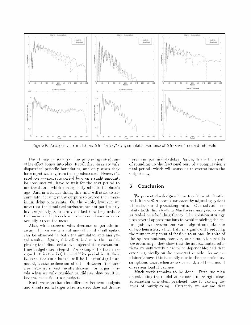
Veri�cation of the Design. The following tablecompares the estimated success rates with those de-rived via simulation, where all chains are run for atleast 10; 000 periods, and success rates are evaluatedevery second.Output Period SR (Analysis) SR (Simulation)Y1 3 11.33 11.50Y2 16 5.50 5.50Y3 5 5.26 5.39Y4 20 5.47 5.79Y5 10 5.39 5.46Y6 5 6.91 6.93Note that the resulting (simulated) system satis�esminimum success rates of all chains, so we have a sat-isfactory solution. If desired, we can improve it bydoling out the excess resource capacity, i.e., by simplyiterating through the design algorithm again.Perhaps more interesting, however, is Figure 8,which compares the simulated and analytic results formultiple periods, assigned to three selected chains.Here, only the periods are changed; the system uti-lization is �xed throughout. Moreover, when we varythe periods for the chain under consideration, we keepthe rest of the system �xed, and use the parametersfrom the solution given above. The simulation runsdisplayed here ran for 10; 000 periods, for the largestperiod under observation (e.g, on the graph, if thelargest period tested is denoted as 200 ms, then thatrun lasted for 2000 seconds). Also, success rates weremeasured over every one-second interval, and the vari-ance in the success-rates (over one-second intervals vs.the mean) were calculated accordingly.The combinatorial comparison allows us to makethe following observations. First, note a chain's suc-cess rate usually increases as its period decreases { upuntil the point where the the system starts to inject asigni�cant \multiplexing tax." Recall that we do notassume the runtime system can multiplex in�nitesimalgranularities of execution time; rather, a task's utiliza-tion is allocated in integral units over each period.Second, the relationship between variance (mea-sured over one-second intervals) and success is nota direct one. Note that for some chains (e.g., �2),success-rate variance tends to increase at both higherand lower periods. This re ects two separate facts, the�rst of which is fairly obvious, and is an artifact of ourmeasurement process. At lower periods (i.e., higherrates), output successes are sampled much more fre-quently. And when a chain truly tends toward havinga uniform output success probability (as longer chainsdo at higher output rates), taking more readings persecond can arbitrarily lead to higher variances. Inother words, the number of successes-per-second forchain �2 converges on having a Binomial distribution,with a variance of �2(1� �2)=T2.

Analysis Simulation

0 20 40 60 80 100 120 140 160 180 2000

1

2

3

4

5

6

Period

Suc

cess

Rat

e

Chain 2 − Success Rate

Analysis Simulation

0 20 40 60 80 100 120 140 160 180 2000

1

2

3

4

5

6

Period

Suc

cess

Rat

e

Chain 3 − Success Rate

Analysis Simulation

0 20 40 60 80 100 120 140 160 180 2000

1

2

3

4

5

6

7

8

Period

Suc

cess

Rat

e

Chain 6 − Success Rate

0 20 40 60 80 100 120 140 160 180 2000

0.5

1

1.5

2

2.5

3

3.5

Var

ianc

e of

suc

cess

rat

e

Period

Chain 2 − Variance

0 20 40 60 80 100 120 140 160 180 2000

0.5

1

1.5

2

2.5

3

Var

ianc

e of

suc

cess

rat

e

Period

Chain 3 − Variance

0 20 40 60 80 100 120 140 160 180 2000

1

2

3

4

5

6

7

8

Var

ianc

e of

suc

cess

rat

e

Period

Chain 6 − Variance

Figure 8: Analysis vs. simulation: SRi for �2,�3,�6; simulated variance of SRi over 1 second intervals.But at large periods (i.e., low processing rates), an-other e�ect comes into play. Recall that tasks are onlydispatched periodic boundaries, and only when theyhave input waiting from their predecessors. Hence, if aproducer overruns its period by even a slight amount,its consumer will have to wait for the next period touse the data { which consequently adds to the data'sage. And in a longer chain, this time will start to ac-cumulate, causing many outputs to exceed their max-imum delay constraints. On the whole, however, wenote that the simulated variances are not particularlyhigh, especially considering the fact that they includethe one-second intervals where measured success ratesactually exceed the mean.Also, while success rates decrease as periods in-crease, the curves are not smooth, and small spikescan be observed in both the simulated and analyti-cal results. Again, this e�ect is due to the \multi-plexing tax" discussed above, injected since execution-time budgets are integral. For example if a task's as-signed utilization is 0.11, and if its period is 10, thenits execution-time budget will be 1 { resulting in anactual, usable utilization of 0.1. However, the suc-cess rates do monotonically decrease for larger peri-ods when we only consider candidates that result inintegral execution-time budgets.Next, we note that the di�erence between analysisand simulation is larger when a period does not divide

maximum permissible delay. Again, this is the resultof rounding up the fractional part of a computation's�nal period, which will cause us to overestimate theoutput's age.6 ConclusionWe presented a design scheme to achieve stochastic,real-time performance guarantees by adjusting systemutilizations and processing rates. Our solution ex-ploits both discrete-time Markovian analysis, as wellas real-time scheduling theory. The solution strategyuses several approximations to avoid modeling the en-tire system; moreover, our search algorithmmakes useof two heuristics, which help in signi�cantly reducingthe number of potential feasible solutions. In spite ofthe approximations, however, our simulation resultsare promising { they show that the approximated solu-tions are su�ciently close to be dependable; and thaterror is typically on the conservative side. As we ex-plained above, this is usually due to the per-period as-sumptions about when a task can end, and the amountof system load it can use.Much work remains to be done. First, we planon extending the model to include a more rigid char-acterization of system overhead, due to varying de-grees of multiplexing. Currently we assume that

execution-time can be allocated in integral units; otherthan that, no speci�c penalty functions are includedfor context-switching, or for network-switch overhead.We also plan on getting better approximations for the\handover-time" between tasks in a chain, which willresult in tighter analytical results. Finally, we plan onbenchmarking \true" per-packet delay times on suit-able LAN-based testbeds, and using the PDFs derivedfrom those benchmarks.References[1] Alan Burns. Preemptive Priority Based Scheduling: AnAppropriate Engineering Approach. In Sang Son, editor,Principles of Real-Time Systems. Prentice Hall, 1994.[2] Alan Demers. Analysis and Simulation of a Fair QueueingAlgorithm. In Proceedings of ACM SIGCOMM, pages 1{12. ACM Press, September 1989.[3] Norival R. Figueira and Joseph Pasquale. Leave-in-Time:A New Service Discipline for Real-Time Communicationsin a Packet-Switching Network. In Proceedings of ACMSIGCOMM, pages 207{218. ACM Press, October 1995.[4] R. Gerber, S. Hong, and M. Saksena. Guaranteeing Real-Time Requirements with Resource-Based Calibration ofPeriodic Processes. IEEE Transactions on Software Engi-neering, 21, July 1995.[5] Pawan Goyal, Xingang Guo, and Harrick M. Vin. A Hi-erarchical CPU Scheduler for Multimedia Operating Sys-tems. In Proceedings of Symposium on Operating SystemsDesign and Implementation (OSDI '96), pages 107{121,October 1996.[6] Pawan Goyal and Harrick M. Vin. Network Algorithmsand Protocol for Multimedia Servers. In Proceedings ofIEEE INFOCOM. IEEE Computer Society Press, March1993.[7] M. Harbour, M. Klein, and J. Lehoczky. Fixed PriorityScheduling of Periodic Tasks with Varying Execution Pri-ority. In Proceedings, IEEE Real-Time Systems Sympo-sium, pages 116{128, December 1991.[8] Ben Kao and Hector Garcia-Molina. Deadline Assignmentin a Distributed Soft Real-Time System. In Proceedings ofInternational Conference on Distributed Computing sys-tems, pages 428{437. IEEE Computer Society Press, May1993.[9] J. P. Lehoczky and S. Ramos-Thuel. An Optimal Al-gorithm for Scheduling Soft-Aperiodic Tasks in Fixed-PriorityPreemptiveSystems. InProceedings of IEEE Real-Time Systems Symposium, pages 110{123. IEEE Com-puter Society Press, December 1992.[10] J. Leung andM. Merill. A Note on the PreemptiveSchedul-ing of Periodic, Real-Time Tasks. Information ProcessingLetters, 11(3):115{118, November 1980.[11] C. Liu and J. Layland. Scheduling Algorithm for Multi-programming in a Hard Real-Time Environment. Journalof the ACM, 20(1):46{61, January 1973.[12] Cli�ord W. Mercer, Stefan Savage, and Hideyuki Tokuda.Processor Capacity Reserves: Operating System Supportfor Multimedia Applications. In Proceedings of IEEEInternational Conference on Multimedia Computing andSystems. IEEE Computer Society Press, May 1994.

[13] A. K. Parekh and G. Gallager. A Generalized ProcessorSharing Approach to Flow Control in Integrated ServicesNetworks - The Single Node Case. In Proceedings of IEEEINFOCOM, pages 915{924. IEEE Computer SocietyPress,March 1992.[14] S. Sathaye and J. Strosnider. A Real-Time SchedulingFramework for Packet-Switched Networks. In Proceedingsof IEEE Real-Time Systems Symposium, pages 182{191.IEEE Computer Society Press, December 1994.[15] D. Seto, J.P. Lehoczky, L. Sha, and K.G. Shin. On TaskSchedulability in Real-Time Control System. In Proceed-ings of IEEE Real-Time Systems Symposium. IEEE Com-puter Society Press, December 1996.[16] Kang G. Shin and Yi-Chieh Chang. A Reservation-BasedAlgorithm for Scheduling Both Periodic and AperiodicReal-Time Tasks. IEEE Transactions on Computers,44:1405{1419, December 1995.[17] Ion Stoica, Hussein Abdel-Wahab, Kevin Je�ay, Sanjoy K.Baruah, Johannes E. Gehrke, and C. Greg Plaxton. A Pro-portional Resource Allocation Algorithm for Real-Time,Time-Shared Systems. In Proceedings of IEEE Real-TimeSystems Symposium, pages 288{299. IEEE Computer So-ciety Press, December 1996.[18] Jun Sun and Jane W.S. Liu. Bounding completion timesof jobs with arbitrary release times and variable executiontimes. In Proceedings of IEEE Real-Time Systems Sympo-sium, pages 2{12. IEEE Computer Society Press, Decem-ber 1996.[19] T. S. Tia, Z. Deng, M. Shankar, M. Storch, J. Sun, L.-C.Wu, and J. W.-S Liu. ProbabilisticPerformanceGuaranteefor Real-Time Tasks with Varying Computation Times. InProceedings of IEEE Real-Time Technology and Applica-tions Symposium, pages 164{173. IEEE Computer SocietyPress, May 1995.[20] K. Tindell, A. Burns, and A. Wellings. Analysis of hardreal-time communication. The Journal of Real-Time Sys-tems, 9, September 1995.[21] David Yates, James Kurose, Don Towsley, and Michael G.Hluchyj. On Per-session End-to-end Delay Distributionsand the Call Admission Problem for Real-time Applica-tions with QOS Requirements. In Proceedings of ACMSIGCOMM. ACM Press, September 1993.[22] Hui Zhang and D. Ferrari. Rate-controlled static-priorityqueueing. In Proceedings of IEEE INFOCOM. IEEE Com-puter Society Press, September 1993.[23] Hui Zhang and Edward W. Knightly. Providing End-to-End StatisticalPerformanceGuaranteeswith Bounding In-terval Dependent Stochastic Models. In ACM SIGMET-RICS. ACM Press, May 1994.[24] Lixia Zhang. VirtualClock : A New Tra�c control Algo-rithm for Packet Switching Networks. In Proceedings ofACM SIGCOMM, pages 19{29. ACM Press, September1990.[25] Zhi-Li Zhang, Don Towsley, and Jim Kurose. StatisticalAnalysis of Generalized Processor Sharing Scheduling Dis-cipline. In Proceedings of ACM SIGCOMM, pages 68{77.ACM Press, August 1994.