Performance assessment of the Ocean Falls Wave Energy ...

t

Performance assessment of the Ocean Falls Wave Energy Converter A solution for electrical power production in the future

R. van den Kerkhoff

Del

ft U

niv

ersi

ty o

f Te

chn

olo

gy

Challenge the future

Performance assessment of the Ocean Falls Wave Energy Converter

A solution for electrical power production in the future

By

Roy-Matthieu van den Kerkhoff

in partial fulfilment of the requirements for the degree of

Master of Science

in Structural Engineering at the Delft University of Technology

Student number: 4224825 Project duration: September 1, 2018 – June 20, 2019 Thesis committee: Prof. ir. A.Q.C. van der Horst TU Delft Dr. ir. drs. C.R. Braam TU Delft

Dr. ir. J.D. Bricker TU Delft Dr. ir. A.J. Laguna TU Delft

Ir. E. ten Oever BAM Infraconsult b.v.

An electronic version of this thesis is available at http://repository.tudelft.nl/

III

Abstract There is a growing demand for renewable sources of energy of which wave energy conversion is one. The Ocean Falls wave energy converter is an oscillating water column (OWC) system invented by BAM Infraconsult b.v. This system differs from conventional OWC systems since it includes a connection tube and an adjustable back wall. The OWC system is a resonance system for which the highest efficiency is obtained once the natural frequency matches the (average) incoming wave frequency. A numerical frequency domain model of the OWC system is developed to evaluate hydrodynamic interactions and performance capabilities. This ‘’parametric model’’ applies 3D numerical diffraction software ANSYS AQWA to calculate the hydrodynamic coefficients and excitation forces on the oscillating body of the OWC system. The model includes a Python script which converts these coefficients into power output and system efficiency. The system behavior depends on the structural geometry for which 13 designs with different geometries are made. For each design the effects on system performance and the first system natural frequency are investigated aiming to find a preferred geometry and design. The system performance represents the system efficiency which is defined as the power available to the power take-off system (PTO) divided by the available wave energy flux. The parameters defining the geometry of the Ocean Falls OWC system are the height of the connection tube 𝐴, width of the air chamber 𝐵 and the length of the connection tube 𝐿. All designs are compared with respect to a base case geometry; 𝐴 = 5.32 m, 𝐵 = 5.37 m, 𝐿 = 13.05 m. In theory and with respect to the base case a value of 𝐴 > 5.32 m reduces performance and a value of 𝐴 < 5.32 m improves performance. In case 𝐵 > 5.37 m the performance improves while 𝐵 < 5.37 m reduces performance. Likewise, 𝐿 > 13.05 m improves performance and 𝐿 < 13.05 m reduces performance. However, the performance depends on the wave statistics which are site specific. The system efficiency is calculated for both regular- and irregular waves. For the designs with variable 𝐴 the system efficiency for irregular waves ranges from 25.5% to 33%. For the designs with variable 𝐵 the system efficiency ranges from 22% to 36%. The efficiency for the designs with variable 𝐿 ranges from 27% to 33.5%. A CFD model is applied to assess the validity of the linearized parametric model. For open chamber conditions where there is no energy extraction, the water surface elevation and air chamber pressure obtained from both models are similar. For a range of wave periods the parametric model underestimates the resonance period and the internal water surface elevation. For closed chamber conditions the parametric model underestimates the air chamber pressure but shows a similar elevation of the internal water surface. For partly closed chamber conditions the parametric model underestimates both the internal water surface elevation and the air chamber pressure. Based on the maximum amplitudes of the water surface elevation and air pressure in the air chamber, the parametric model differs on average 15-20% from the CFD model. To decide on a design to be applied for the conceptual design of the Ocean Falls a decision is made based on three criteria: system performance, constructability and cost effectiveness. At a chosen project location, the power production of each design is calculated while considering an available wave energy flux of 10.1 𝑘𝑊/𝑚. The power production of the base case equals 2.6 𝑘𝑊/𝑚 which is equivalent to 25% efficiency. Including an adjustable back wall improves the system efficiency to 37%. Secondly constructability aspects e.g. required manhours, concrete, reinforcement are calculated for each design. Finally, a decision is made based on the cost effectiveness in terms of Levelized Cost of Electricity (LCOE). The LCOE of the preferred design equals 0.320 €/kWh (without the adjustable back wall) which is comparable to one of the best performing WEC systems at the chosen project location. The conceptual design of the Ocean Falls showed that the structure fulfills both structural and performance requirements.

V

Acknowledgements This thesis is the result of my graduation internship at BAM Infraconsult b.v. as final part of obtaining a master’s degree for the program Structural Engineering at the Delft University of Technology. I would like to thank several people for their contributions during my master thesis project. Firstly, I would like to thank my professor Aad van der Horst and my daily supervisor René Braam for their guidance, interest and motivation. Input from your field of expertise has been a great contribution to this project. Thanks to Jeremy Bricker and Antonio Laguna for the guidance and valuable input from your fields of expertise. I owe a great debt to the inventor of the Ocean Falls concept Erik ten Oever and I am grateful for the opportunity to work on this subject and that you were willing to be my mentor during my master thesis. I would also like to thank Markus Muttray for his support and assistance. In special I would like to thank my dear friend Ikbal Kelkitli for his support and interest during this project. Additionally, I would like to thank the entire Coastal department of BAM Infraconsult b.v. for their interest, support and giving me the opportunity to work at the company. Finally, many thanks go out to my dear friends and family that always supported, motivated and challenged me to strive for the best possible.

R. van den Kerkhoff Delft, June 2019

VI

Contents

Abstract .......................................................................................................................................................... III

Acknowledgements ......................................................................................................................................... IV

1 Introduction .................................................................................................................................................. 1

1.1 Motivation .................................................................................................................................................... 1

1.2 Introduction to Ocean Falls .......................................................................................................................... 1

1.3 Current status of the Ocean Falls ................................................................................................................. 2

1.4 Problem definition ........................................................................................................................................ 2 1.4.1 Research questions ............................................................................................................................... 2 1.4.2 Project scope ........................................................................................................................................ 3

1.5 Methodology ................................................................................................................................................ 4

2 Literature review ........................................................................................................................................... 5

2.1 Chapter summary ......................................................................................................................................... 5

2.2 Wave energy conversion technology ............................................................................................................ 5

2.2 Wave energy ................................................................................................................................................. 6

2.3 Oscillating Water Column system................................................................................................................. 6 2.3.1 Working principle ................................................................................................................................. 6 2.3.2 Type of OWC systems ........................................................................................................................... 6

2.4 Modelling of OWC systems ........................................................................................................................... 8 2.4.1 Analytical modelling ............................................................................................................................. 8 2.4.2 Numerical modelling ............................................................................................................................ 9 2.4.3 Physical modelling ................................................................................................................................ 9 2.4.4 Applied models ..................................................................................................................................... 9

2.5 The Ocean Falls system............................................................................................................................... 10 2.5.1 Working principle ............................................................................................................................... 10 2.5.2 Phenomena affecting the system efficiency ....................................................................................... 10 2.5.3 Forcing on the rigid body .................................................................................................................... 11 2.5.4 Regular waves vs irregular waves ....................................................................................................... 12

2.6 Equations of the Ocean Falls system .......................................................................................................... 14 2.6.1 Formulating the equations of motion ................................................................................................ 14 2.6.2 Linear turbine ..................................................................................................................................... 16 2.6.3 Radiation forcing ................................................................................................................................ 17 2.6.4 Solutions in the frequency domain ..................................................................................................... 17 2.6.5 System natural frequency ................................................................................................................... 18 2.6.6 Power obtained from irregular waves ................................................................................................ 19 2.6.7 System efficiency ................................................................................................................................ 20

2.7 Design of OWC systems .............................................................................................................................. 21

3 Performance assessment of the Ocean falls ................................................................................................ 22

3.1 Introduction and chapter outline ................................................................................................................ 22

3.2 Parametric model - Python ......................................................................................................................... 22 3.2.1 Objective ............................................................................................................................................. 22 3.2.2 Method ............................................................................................................................................... 22 3.2.3 Results ................................................................................................................................................ 23

VII

3.3 Parametric model - ANSYS AQWA .............................................................................................................. 23 3.3.1 Objective ............................................................................................................................................. 23 3.3.2 Method ............................................................................................................................................... 23 3.3.3 Results ................................................................................................................................................ 24 3.3.4 Conclusion .......................................................................................................................................... 25

3.4 Piston position ............................................................................................................................................ 25 3.4.1 Objective ............................................................................................................................................. 25 3.4.2 Method ............................................................................................................................................... 25 3.4.3 Results ................................................................................................................................................ 25 3.4.4 Conclusion .......................................................................................................................................... 26

3.5 The effect of hydrodynamic coefficients on the system response .............................................................. 26 3.5.1 Objective ............................................................................................................................................. 26 3.5.2 Method ............................................................................................................................................... 26 3.5.3 Results ................................................................................................................................................ 27

3.6 The effect of geometry on the system response ......................................................................................... 28 3.6.1 Objective ............................................................................................................................................. 28 3.6.2 Method ............................................................................................................................................... 28 3.6.3 Results ................................................................................................................................................ 28 3.6.4 Conclusion .......................................................................................................................................... 29 3.6.5 Method ............................................................................................................................................... 30 3.6.6 Results ................................................................................................................................................ 30 3.6.7 Conclusion .......................................................................................................................................... 32

3.7 The effect of irregular waves the system performance .............................................................................. 33 3.7.1 Objective ............................................................................................................................................. 33 3.7.2 Method ............................................................................................................................................... 33 3.7.3 Results ................................................................................................................................................ 33 3.7.4 Conclusion .......................................................................................................................................... 33

3.8 System performance of the Ocean Falls ..................................................................................................... 34 3.8.1 Objective ............................................................................................................................................. 34 3.8.2 Method ............................................................................................................................................... 34 3.8.3 Results ................................................................................................................................................ 35 3.8.4 Results ................................................................................................................................................ 36 3.8.5 Conclusion .......................................................................................................................................... 38

3.9 CFD model .................................................................................................................................................. 39 3.9.1 Objective ............................................................................................................................................. 39 3.9.2 Method ............................................................................................................................................... 39 3.9.3 Results ................................................................................................................................................ 41

3.10 Deciding on a design................................................................................................................................. 52 3.10.1 Objective ........................................................................................................................................... 52 3.10.2 Method ............................................................................................................................................. 52 3.10.3 Results .............................................................................................................................................. 53 3.10.4 Method ............................................................................................................................................. 54 3.10.5 Results .............................................................................................................................................. 54 3.10.6 Conclusion ........................................................................................................................................ 56

4 Conceptual design of the Ocean Falls .......................................................................................................... 60

4.1 Introduction and chapter outline ................................................................................................................ 60

4.2 Structural performance assessment ........................................................................................................... 60 4.2.1 Design phases ..................................................................................................................................... 60 4.2.3 Design checks ..................................................................................................................................... 66

4.3 Strength calculation ................................................................................................................................... 72

VIII

4.4 Feasibility of the Ocean Falls OWC system ................................................................................................. 79

5 Discussion and conclusions .......................................................................................................................... 80

5.1 Discussion ................................................................................................................................................... 80 5.1.1 Parametric model ............................................................................................................................... 80 5.1.2 CFD model .......................................................................................................................................... 81 5.1.3 Conceptual design .............................................................................................................................. 82

5.2 Conclusions ................................................................................................................................................. 83

5.3 Recommendations for further research...................................................................................................... 87

6 Bibliography ................................................................................................................................................ 89

Appendix A ..................................................................................................................................................... 93

Figures and tables ............................................................................................................................................ 93

Nomenclature ................................................................................................................................................... 95

A.1 Wave energy .............................................................................................................................................. 98 A.1.1 Linear wave theory ............................................................................................................................. 98 A.1.2 Wave energy – Regular waves............................................................................................................ 98 A.1.3 Wave energy – Irregular waves .......................................................................................................... 99 A.1.3 Wave energy – Spectral irregular waves .......................................................................................... 100

A.2 Construction methods .............................................................................................................................. 100 A.2.1 Existing methods .............................................................................................................................. 100 A.2.2 construction phase ........................................................................................................................... 100 A.2.3 Land transportation phase ............................................................................................................... 101 A.2.4 Land – water phase .......................................................................................................................... 101 A.2.5 Water phase ..................................................................................................................................... 102

A.3.1 ANSYS AQWA ........................................................................................................................................ 104 A.3.1.1 Model set-up ................................................................................................................................. 104 A.3.1.2 Effect of wave diffraction on the hydrodynamic coefficients ....................................................... 105

A.3.2 Piston position ....................................................................................................................................... 106

A.3.3 Hydrodynamic coefficients .................................................................................................................... 107

A.3.4 The effect of geometry – Parametric model (Python) ........................................................................... 108

A.3.5 Effect of the sea-state ........................................................................................................................... 111

A.3.6 System performance of the Ocean Falls ................................................................................................ 111

A.3.7 CFD model ............................................................................................................................................. 113 A.3.7.1 Boundary conditions and model set-up ........................................................................................ 113 A.3.7.2 Wave reflection analysis................................................................................................................ 115 A.3.7.3 CFD model – model scale experiments ......................................................................................... 115 A.3.7.4 Validity of the parametric model .................................................................................................. 115

A.3.8 Deciding on a design ............................................................................................................................. 119 A.3.8.1 Wave climate data project location .............................................................................................. 119 A.3.8.1 Cost calculation ............................................................................................................................. 120

A.4 Conceptual design .................................................................................................................................... 122 A.4.1 Wave forcing (Goda) ........................................................................................................................ 122 A.4.2 CFD analysis ...................................................................................................................................... 122 A.4.3 Conceptual design drawings............................................................................................................. 123

A.5 Python script - Parametric model ............................................................................................................. 125

1

1 Introduction Wave energy stands out among other renewable energy sources for its high potential and high energy density of which the latter is the highest of all renewables according to Lopez [66]. According to Sheng [1] the total wave energy is estimated at around 32000 TWh per year which is more than the worldwide electricity consumption of 24345 TWh per year. This shows that wave energy has a high potential as a renewable source of energy. Generating energy from the ocean is a concept know for many years, but the implementation of wave energy conversion systems is still limited. Wave energy is currently in its pre-commercial phase and work is ongoing on the evaluation of the wave energy potential and the detailed characterization of this renewable energy resource. This research aims to contribute to this work by investigating the oscillating water column wave energy converter called ‘’The Ocean Falls’’.

1.1 Motivation This research is motivated by the development of new alternatives and the improvement of the knowledge on wave energy conversion. The Ocean Falls is a Wave Energy Converter (WEC) based on the Oscillating Water Column (OWC) principle. The potential of WEC systems in improving the production of energy and benefit human life is substantial. In the recent years many wave energy converters have been developed and shown their potential, unfortunately these systems are rarely implemented. The greatest challenges are a reduction of the construction costs, reliability of performance and ways to improve efficiency.

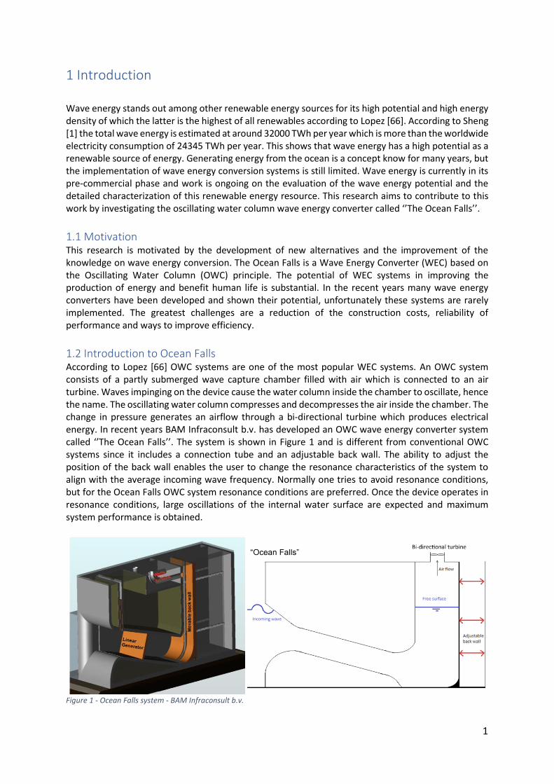
1.2 Introduction to Ocean Falls According to Lopez [66] OWC systems are one of the most popular WEC systems. An OWC system consists of a partly submerged wave capture chamber filled with air which is connected to an air turbine. Waves impinging on the device cause the water column inside the chamber to oscillate, hence the name. The oscillating water column compresses and decompresses the air inside the chamber. The change in pressure generates an airflow through a bi-directional turbine which produces electrical energy. In recent years BAM Infraconsult b.v. has developed an OWC wave energy converter system called ‘’The Ocean Falls’’. The system is shown in Figure 1 and is different from conventional OWC systems since it includes a connection tube and an adjustable back wall. The ability to adjust the position of the back wall enables the user to change the resonance characteristics of the system to align with the average incoming wave frequency. Normally one tries to avoid resonance conditions, but for the Ocean Falls OWC system resonance conditions are preferred. Once the device operates in resonance conditions, large oscillations of the internal water surface are expected and maximum system performance is obtained.

Figure 1 - Ocean Falls system - BAM Infraconsult b.v.

2

1.3 Current status of the Ocean Falls The Ocean Falls wave energy converter is not ready to be implemented and considered as an alternative source of energy, since its performance and structural reliability have not been verified. In this research the system performance represents the system efficiency which is defined as the power available to the power take-off system (PTO) divided by the available wave energy flux. Topics to be investigated before the Ocean Falls can be implemented are:

• System performance for irregular waves

• System performance for full-scale geometry

• Optimization of geometry with respect to system performance

• Constructability, construction costs and cost effectiveness

• Structural performance

• Risk assessment

Figure 2 shows the Technology Readiness Levels (TRL) of the project obtained from Kruit [50]. To date the concept of the Ocean Falls system is formulated and basic principles have been validated. Currently the Ocean Falls is in between TRL 3-4, where the system is validated by experiments with a scale model prototype.

Figure 2 - Project stages of development [50]

1.4 Problem definition Previous research is done by BAM Infraconsult b.v. and Kelkitli [7] investigating the dynamic effects of the system and validation of a numerical model by performing model scale experiments for regular waves. This research will contribute by making an assessment on the system performance and structural performance of the Ocean Falls OWC system.

1.4.1 Research questions The aim of this research is to answer the main research question regarding the technical feasibility of the Ocean Falls. The main question is divided into several research questions.

‘’How to assess the technical feasibility of the Ocean Falls OWC system based on performance and structural requirements?’’

I. ‘’What is the effect of the geometry; width of the air chamber, height of the connection tube

and length of the connection tube on the system performance?’’

II. ‘’What is the effect of irregular waves on the system performance?’’

III. ‘’What is the extent of validity of a linearized parametric model?’’

IV. ‘’How to obtain an “optimal” design based on both system performance and constructability aspects”?

V. “How to make a conceptual design of the Ocean Falls which fulfills both structural and

performance requirements?”

3

1.4.2 Project scope

Part 1: Literature review A literature review is done to investigate different type of OWC systems, forcing on the system, irregular wave characteristics, methods for modelling of OWC systems, construction technology aspects and design conditions of OWC systems. An integral part of the literature review is the explanation of equations required to model the Ocean Falls system.

Part 2A: Performance assessment of the Ocean Falls A parametric model is developed to calculate the system performance in terms of power output and system efficiency. The model applies numerical diffraction software ANSYS AQWA. The hydrodynamic coefficients obtained from the ANSYS AQWA model provide insight in the system behavior. A python model converts these coefficients into a value of system performance. The scope of the performance assessment includes:

- Development of a Python model including the differential equations of the system - Development of a diffraction model with numerical diffraction software ANSYS AQWA - Development of a parametric model which includes both the Python model and the ANSYS

AQWA model of the Ocean Falls. - Investigate the effect of different piston positions in the ANSYS AQWA model - Development of different designs each with a different geometry in ANSYS DesignModeler - Observe and explain the effect of geometry on the system behavior with the parametric model - Investigate the effect of regular- and irregular waves on the system performance with the

parametric model - Development of a CFD model in ANSYS Fluent - Assess the validity of the CFD model with model scale experiments - Assess the validity of the parametric model with the CFD model

Part 2B: Concept case study To decide on a design a concept case study is applied. In the case study each design is assessed on system performance, constructability and cost effectiveness aiming to find a preferred geometry and design. The preferred design will be applied for the conceptual design of the Ocean Falls. The scope of the concept case study includes:

- Decide on a project location - Calculate the energy production of each design at the project location - Investigate the constructability of each design - Calculate the cost of each design - Calculate the cost effectiveness of each design - Decide on a design

Part 3: Conceptual design A conceptual design is developed based on both structural and performance requirements. The conceptual design will be used to assess the structural performance and decide whether the structure can be built and is able to withstand the loading. The project scope of the conceptual design includes:

- Perform design checks while considering different project phases - Define structural requirements, modifications and improvements of the design - Assess the technical- and economic feasibility of the Ocean Falls

4

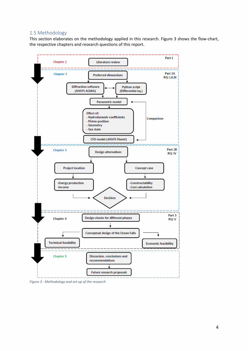
1.5 Methodology This section elaborates on the methodology applied in this research. Figure 3 shows the flow-chart, the respective chapters and research questions of this report.

Figure 3 - Methodology and set-up of the research

5

2 Literature review

2.1 Chapter summary This chapter provides background information and elaborates on the working principle of OWC systems. Section 2.2 provides the reader with information about wave energy conversion technology. In section 2.3 the working principle of an OWC system is explained and different type of OWC systems are discussed. Section 2.4 elaborates on the modelling of OWC systems and the models applied for this research. Section 2.5 elaborates on the working principle and type of forcing on the Ocean Falls system. This section also includes information about regular- and irregular waves. Section 2.6 provides the equations to model the Ocean Falls OWC system. Section 2.7 explains the design process of OWC systems in general.

2.2 Wave energy conversion technology Wave energy conversion (WEC) technology started with Yoshio Masuda who is nowadays known as the father of modern wave energy technology [4]. Masuda was since 1940 involved in wave energy conversion and in 1965 he became the first inventor of an OWC system [4]. In 1976 Masuda invented and constructed a large device called Kaimei which was installed in the sea and was equipped with air turbines. During the oil crisis in 1973 renewable sources of energy became attractive for the international scientific community. In 1975 the British Government started a research and development program in WEC technology followed by the Norwegian Government aiming to improve the knowledge [4]. Until the 1990s prototypes were installed on the coast of England and Norway but the activity in Europe remained on an academic level [4]. Only a single successful OWC prototype was in 1991 constructed near the shore of Scotland. The major gaps for implementation of OWC systems during the 1970s and 1980s were due to a lack of knowledge about the physical processes in these systems [4]. The development of numerical modelling was a large contributor to the knowledge on OWC systems. However, the results were still considered unreliable since the numerical models did not include hydrodynamic effects and other non-linear phenomena. The use of physical models in scale experiments improved the knowledge about these effects which resulted in more reliable WEC systems. When in 1991 the decision was made by the European Commission to include WEC technology in the R&D program on renewable energy; wave energy projects became more attractive. In the past decade many European- and international conferences about wave energy were organized aiming to improve the knowledge about wave energy conversion systems. To date no WEC systems survived the growth to commercial stage since the costs for energy production exceeds the returns from selling energy. The economics of WEC show that costs for energy production with WEC systems is much higher than compared to offshore wind. According to van der Jagt [65] a reduction of costs is expected after a successful concept enters large scale production. The main reasons for lack of implementation of WEC systems are the variability in energy resource and system inefficiency. One of the requirements of an OWC system to be efficient is that it should operate in near-resonance conditions [4]. Many inventors ignored this and assumed that the systems were quasi-static and not dynamic. This is one of the main reasons why many WEC systems were considered unreliable, inefficient and have failed in the past. Many WEC research and development goals remain to be accomplished [69]. These include: cost reduction, efficiency and reliability, identification of suitable sites, interconnection with the utility grid, understanding of the impact of WEC systems on the marine environment, the ability of WEC systems to survive in the marine environment as well as weather effects over the service lifetime.

6

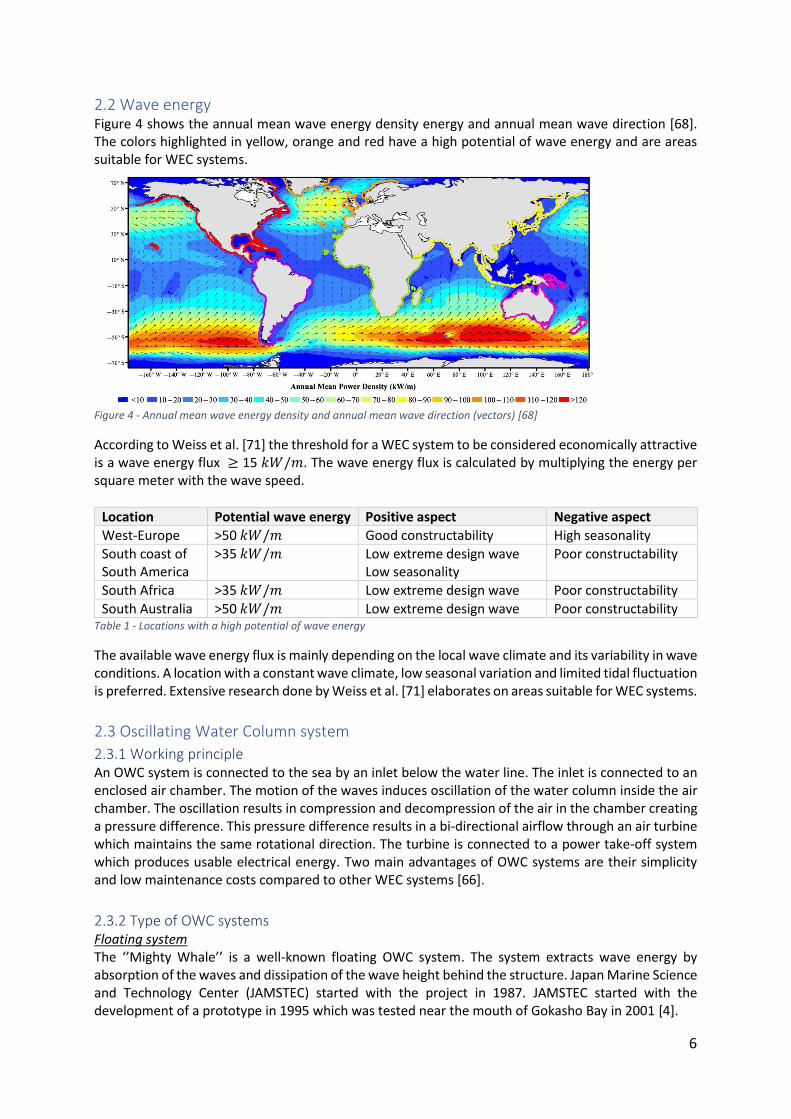
2.2 Wave energy Figure 4 shows the annual mean wave energy density energy and annual mean wave direction [68]. The colors highlighted in yellow, orange and red have a high potential of wave energy and are areas suitable for WEC systems.

Figure 4 - Annual mean wave energy density and annual mean wave direction (vectors) [68]

According to Weiss et al. [71] the threshold for a WEC system to be considered economically attractive is a wave energy flux ≥ 15 𝑘𝑊/𝑚. The wave energy flux is calculated by multiplying the energy per square meter with the wave speed.

Location Potential wave energy Positive aspect Negative aspect

West-Europe >50 𝑘𝑊/𝑚 Good constructability High seasonality

South coast of South America

>35 𝑘𝑊/𝑚 Low extreme design wave Low seasonality

Poor constructability

South Africa >35 𝑘𝑊/𝑚 Low extreme design wave Poor constructability

South Australia >50 𝑘𝑊/𝑚 Low extreme design wave Poor constructability Table 1 - Locations with a high potential of wave energy

The available wave energy flux is mainly depending on the local wave climate and its variability in wave conditions. A location with a constant wave climate, low seasonal variation and limited tidal fluctuation is preferred. Extensive research done by Weiss et al. [71] elaborates on areas suitable for WEC systems.

2.3 Oscillating Water Column system

2.3.1 Working principle An OWC system is connected to the sea by an inlet below the water line. The inlet is connected to an enclosed air chamber. The motion of the waves induces oscillation of the water column inside the air chamber. The oscillation results in compression and decompression of the air in the chamber creating a pressure difference. This pressure difference results in a bi-directional airflow through an air turbine which maintains the same rotational direction. The turbine is connected to a power take-off system which produces usable electrical energy. Two main advantages of OWC systems are their simplicity and low maintenance costs compared to other WEC systems [66].

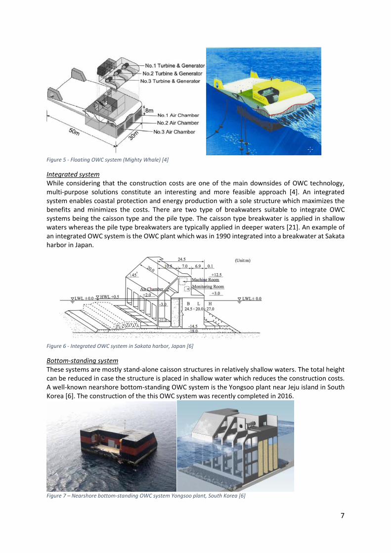
2.3.2 Type of OWC systems Floating system The ‘’Mighty Whale’’ is a well-known floating OWC system. The system extracts wave energy by absorption of the waves and dissipation of the wave height behind the structure. Japan Marine Science and Technology Center (JAMSTEC) started with the project in 1987. JAMSTEC started with the development of a prototype in 1995 which was tested near the mouth of Gokasho Bay in 2001 [4].

7

Figure 5 - Floating OWC system (Mighty Whale) [4]

Integrated system While considering that the construction costs are one of the main downsides of OWC technology, multi-purpose solutions constitute an interesting and more feasible approach [4]. An integrated system enables coastal protection and energy production with a sole structure which maximizes the benefits and minimizes the costs. There are two type of breakwaters suitable to integrate OWC systems being the caisson type and the pile type. The caisson type breakwater is applied in shallow waters whereas the pile type breakwaters are typically applied in deeper waters [21]. An example of an integrated OWC system is the OWC plant which was in 1990 integrated into a breakwater at Sakata harbor in Japan.

Figure 6 - Integrated OWC system in Sakata harbor, Japan [6]

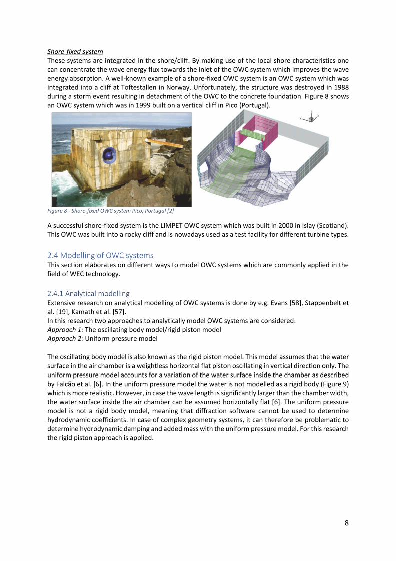
Bottom-standing system These systems are mostly stand-alone caisson structures in relatively shallow waters. The total height can be reduced in case the structure is placed in shallow water which reduces the construction costs. A well-known nearshore bottom-standing OWC system is the Yongsoo plant near Jeju island in South Korea [6]. The construction of the this OWC system was recently completed in 2016.

Figure 7 – Nearshore bottom-standing OWC system Yongsoo plant, South Korea [6]

8

Shore-fixed system These systems are integrated in the shore/cliff. By making use of the local shore characteristics one can concentrate the wave energy flux towards the inlet of the OWC system which improves the wave energy absorption. A well-known example of a shore-fixed OWC system is an OWC system which was integrated into a cliff at Toftestallen in Norway. Unfortunately, the structure was destroyed in 1988 during a storm event resulting in detachment of the OWC to the concrete foundation. Figure 8 shows an OWC system which was in 1999 built on a vertical cliff in Pico (Portugal).

Figure 8 - Shore-fixed OWC system Pico, Portugal [2]

A successful shore-fixed system is the LIMPET OWC system which was built in 2000 in Islay (Scotland). This OWC was built into a rocky cliff and is nowadays used as a test facility for different turbine types.

2.4 Modelling of OWC systems This section elaborates on different ways to model OWC systems which are commonly applied in the field of WEC technology.

2.4.1 Analytical modelling Extensive research on analytical modelling of OWC systems is done by e.g. Evans [58], Stappenbelt et al. [19], Kamath et al. [57]. In this research two approaches to analytically model OWC systems are considered: Approach 1: The oscillating body model/rigid piston model Approach 2: Uniform pressure model

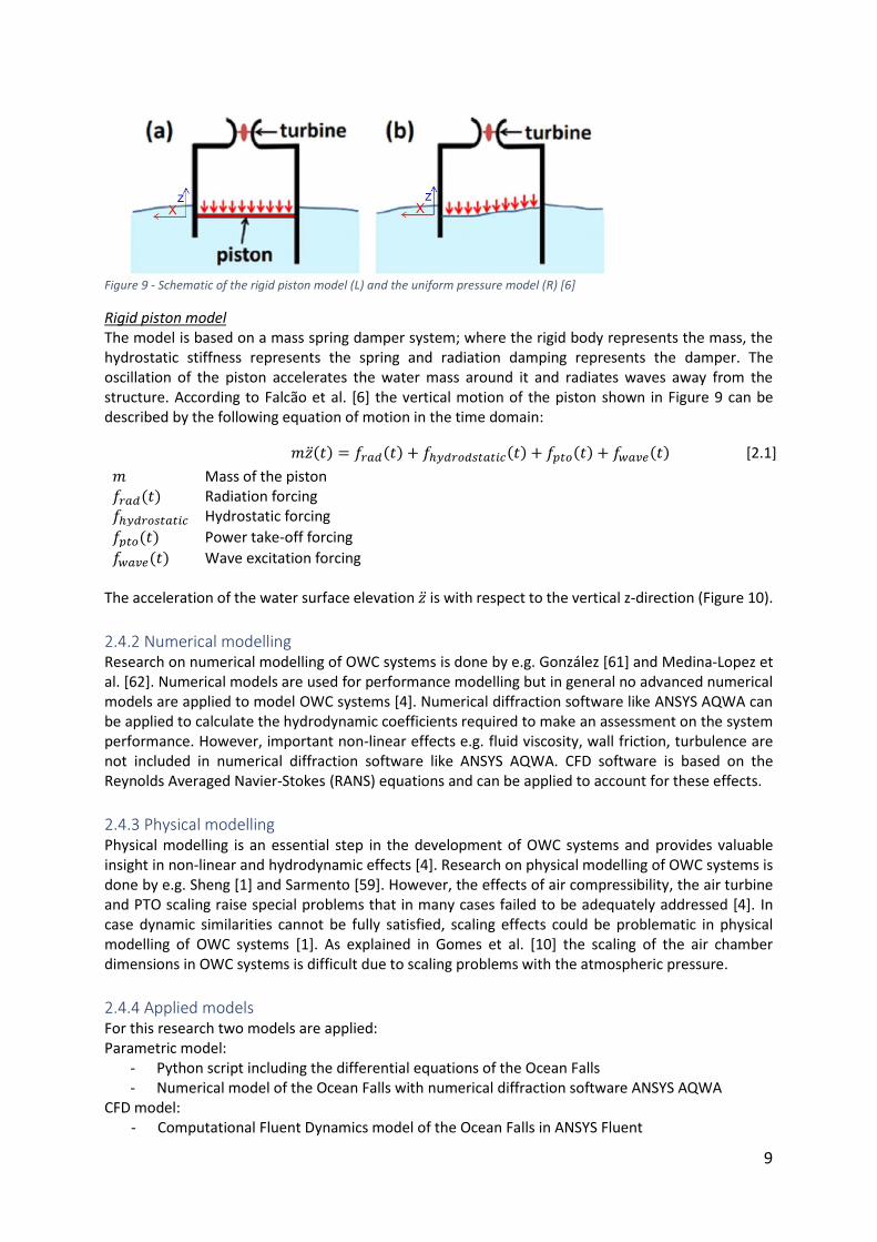
The oscillating body model is also known as the rigid piston model. This model assumes that the water surface in the air chamber is a weightless horizontal flat piston oscillating in vertical direction only. The uniform pressure model accounts for a variation of the water surface inside the chamber as described by Falcao et al. [6]. In the uniform pressure model the water is not modelled as a rigid body (Figure 9) which is more realistic. However, in case the wave length is significantly larger than the chamber width, the water surface inside the air chamber can be assumed horizontally flat [6]. The uniform pressure model is not a rigid body model, meaning that diffraction software cannot be used to determine hydrodynamic coefficients. In case of complex geometry systems, it can therefore be problematic to determine hydrodynamic damping and added mass with the uniform pressure model. For this research the rigid piston approach is applied.

9

𝑚��(𝑡) = 𝑓𝑟𝑎𝑑(𝑡) + 𝑓ℎ𝑦𝑑𝑟𝑜𝑑𝑠𝑡𝑎𝑡𝑖𝑐(𝑡) + 𝑓𝑝𝑡𝑜(𝑡) + 𝑓𝑤𝑎𝑣𝑒(𝑡) [2.1]

[2.2]

Figure 9 - Schematic of the rigid piston model (L) and the uniform pressure model (R) [6]

Rigid piston model The model is based on a mass spring damper system; where the rigid body represents the mass, the hydrostatic stiffness represents the spring and radiation damping represents the damper. The oscillation of the piston accelerates the water mass around it and radiates waves away from the structure. According to Falcao et al. [6] the vertical motion of the piston shown in Figure 9 can be described by the following equation of motion in the time domain:

𝑚 Mass of the piston 𝑓𝑟𝑎𝑑(𝑡) Radiation forcing 𝑓ℎ𝑦𝑑𝑟𝑜𝑠𝑡𝑎𝑡𝑖𝑐 Hydrostatic forcing

𝑓𝑝𝑡𝑜(𝑡) Power take-off forcing

𝑓𝑤𝑎𝑣𝑒(𝑡) Wave excitation forcing The acceleration of the water surface elevation �� is with respect to the vertical z-direction (Figure 10).

2.4.2 Numerical modelling Research on numerical modelling of OWC systems is done by e.g. Gonzalez [61] and Medina-Lopez et al. [62]. Numerical models are used for performance modelling but in general no advanced numerical models are applied to model OWC systems [4]. Numerical diffraction software like ANSYS AQWA can be applied to calculate the hydrodynamic coefficients required to make an assessment on the system performance. However, important non-linear effects e.g. fluid viscosity, wall friction, turbulence are not included in numerical diffraction software like ANSYS AQWA. CFD software is based on the Reynolds Averaged Navier-Stokes (RANS) equations and can be applied to account for these effects.

2.4.3 Physical modelling Physical modelling is an essential step in the development of OWC systems and provides valuable insight in non-linear and hydrodynamic effects [4]. Research on physical modelling of OWC systems is done by e.g. Sheng [1] and Sarmento [59]. However, the effects of air compressibility, the air turbine and PTO scaling raise special problems that in many cases failed to be adequately addressed [4]. In case dynamic similarities cannot be fully satisfied, scaling effects could be problematic in physical modelling of OWC systems [1]. As explained in Gomes et al. [10] the scaling of the air chamber dimensions in OWC systems is difficult due to scaling problems with the atmospheric pressure.

2.4.4 Applied models For this research two models are applied: Parametric model: - Python script including the differential equations of the Ocean Falls - Numerical model of the Ocean Falls with numerical diffraction software ANSYS AQWA CFD model:

- Computational Fluent Dynamics model of the Ocean Falls in ANSYS Fluent

10

2.5 The Ocean Falls system

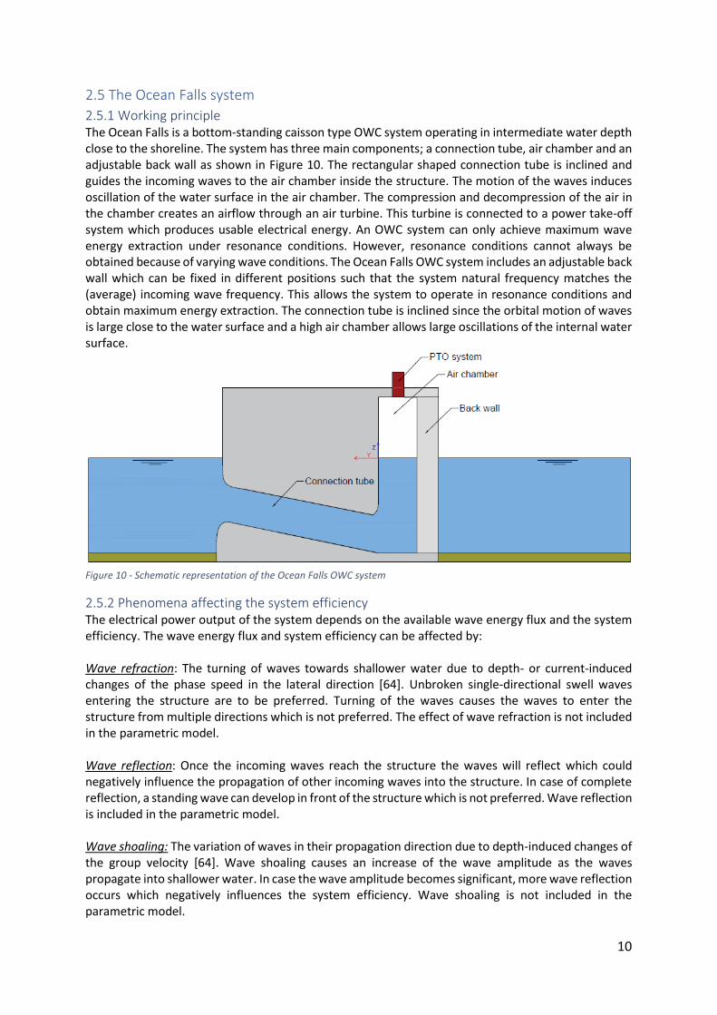
2.5.1 Working principle The Ocean Falls is a bottom-standing caisson type OWC system operating in intermediate water depth close to the shoreline. The system has three main components; a connection tube, air chamber and an adjustable back wall as shown in Figure 10. The rectangular shaped connection tube is inclined and guides the incoming waves to the air chamber inside the structure. The motion of the waves induces oscillation of the water surface in the air chamber. The compression and decompression of the air in the chamber creates an airflow through an air turbine. This turbine is connected to a power take-off system which produces usable electrical energy. An OWC system can only achieve maximum wave energy extraction under resonance conditions. However, resonance conditions cannot always be obtained because of varying wave conditions. The Ocean Falls OWC system includes an adjustable back wall which can be fixed in different positions such that the system natural frequency matches the (average) incoming wave frequency. This allows the system to operate in resonance conditions and obtain maximum energy extraction. The connection tube is inclined since the orbital motion of waves is large close to the water surface and a high air chamber allows large oscillations of the internal water surface.

Figure 10 - Schematic representation of the Ocean Falls OWC system

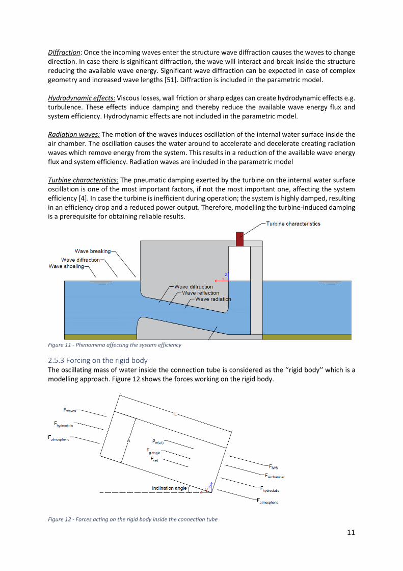
2.5.2 Phenomena affecting the system efficiency The electrical power output of the system depends on the available wave energy flux and the system efficiency. The wave energy flux and system efficiency can be affected by: Wave refraction: The turning of waves towards shallower water due to depth- or current-induced changes of the phase speed in the lateral direction [64]. Unbroken single-directional swell waves entering the structure are to be preferred. Turning of the waves causes the waves to enter the structure from multiple directions which is not preferred. The effect of wave refraction is not included in the parametric model.

Wave reflection: Once the incoming waves reach the structure the waves will reflect which could negatively influence the propagation of other incoming waves into the structure. In case of complete reflection, a standing wave can develop in front of the structure which is not preferred. Wave reflection is included in the parametric model.

Wave shoaling: The variation of waves in their propagation direction due to depth-induced changes of the group velocity [64]. Wave shoaling causes an increase of the wave amplitude as the waves propagate into shallower water. In case the wave amplitude becomes significant, more wave reflection occurs which negatively influences the system efficiency. Wave shoaling is not included in the parametric model.

11

Diffraction: Once the incoming waves enter the structure wave diffraction causes the waves to change direction. In case there is significant diffraction, the wave will interact and break inside the structure reducing the available wave energy. Significant wave diffraction can be expected in case of complex geometry and increased wave lengths [51]. Diffraction is included in the parametric model. Hydrodynamic effects: Viscous losses, wall friction or sharp edges can create hydrodynamic effects e.g. turbulence. These effects induce damping and thereby reduce the available wave energy flux and system efficiency. Hydrodynamic effects are not included in the parametric model.

Radiation waves: The motion of the waves induces oscillation of the internal water surface inside the air chamber. The oscillation causes the water around to accelerate and decelerate creating radiation waves which remove energy from the system. This results in a reduction of the available wave energy flux and system efficiency. Radiation waves are included in the parametric model

Turbine characteristics: The pneumatic damping exerted by the turbine on the internal water surface oscillation is one of the most important factors, if not the most important one, affecting the system efficiency [4]. In case the turbine is inefficient during operation; the system is highly damped, resulting in an efficiency drop and a reduced power output. Therefore, modelling the turbine-induced damping is a prerequisite for obtaining reliable results.

Figure 11 - Phenomena affecting the system efficiency

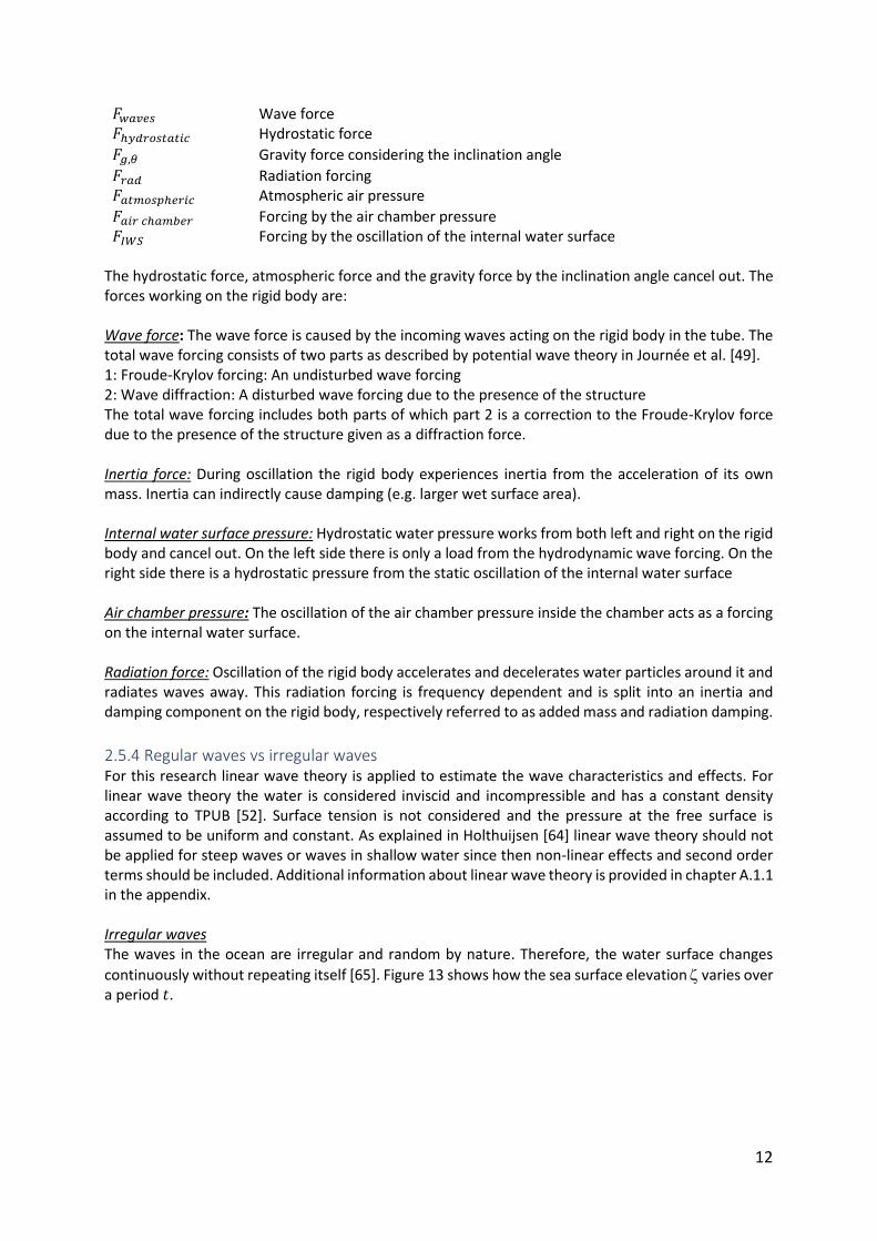
2.5.3 Forcing on the rigid body The oscillating mass of water inside the connection tube is considered as the ‘’rigid body’’ which is a modelling approach. Figure 12 shows the forces working on the rigid body.

Figure 12 - Forces acting on the rigid body inside the connection tube

12

𝐹𝑤𝑎𝑣𝑒𝑠 Wave force 𝐹ℎ𝑦𝑑𝑟𝑜𝑠𝑡𝑎𝑡𝑖𝑐 Hydrostatic force

𝐹𝑔,𝜃 Gravity force considering the inclination angle

𝐹𝑟𝑎𝑑 Radiation forcing 𝐹𝑎𝑡𝑚𝑜𝑠𝑝ℎ𝑒𝑟𝑖𝑐 Atmospheric air pressure

𝐹𝑎𝑖𝑟 𝑐ℎ𝑎𝑚𝑏𝑒𝑟 Forcing by the air chamber pressure 𝐹𝐼𝑊𝑆 Forcing by the oscillation of the internal water surface

The hydrostatic force, atmospheric force and the gravity force by the inclination angle cancel out. The forces working on the rigid body are: Wave force: The wave force is caused by the incoming waves acting on the rigid body in the tube. The total wave forcing consists of two parts as described by potential wave theory in Journée et al. [49]. 1: Froude-Krylov forcing: An undisturbed wave forcing 2: Wave diffraction: A disturbed wave forcing due to the presence of the structure The total wave forcing includes both parts of which part 2 is a correction to the Froude-Krylov force due to the presence of the structure given as a diffraction force. Inertia force: During oscillation the rigid body experiences inertia from the acceleration of its own mass. Inertia can indirectly cause damping (e.g. larger wet surface area). Internal water surface pressure: Hydrostatic water pressure works from both left and right on the rigid body and cancel out. On the left side there is only a load from the hydrodynamic wave forcing. On the right side there is a hydrostatic pressure from the static oscillation of the internal water surface Air chamber pressure: The oscillation of the air chamber pressure inside the chamber acts as a forcing on the internal water surface. Radiation force: Oscillation of the rigid body accelerates and decelerates water particles around it and radiates waves away. This radiation forcing is frequency dependent and is split into an inertia and damping component on the rigid body, respectively referred to as added mass and radiation damping.

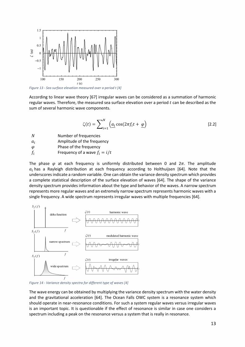
2.5.4 Regular waves vs irregular waves For this research linear wave theory is applied to estimate the wave characteristics and effects. For linear wave theory the water is considered inviscid and incompressible and has a constant density according to TPUB [52]. Surface tension is not considered and the pressure at the free surface is assumed to be uniform and constant. As explained in Holthuijsen [64] linear wave theory should not be applied for steep waves or waves in shallow water since then non-linear effects and second order terms should be included. Additional information about linear wave theory is provided in chapter A.1.1 in the appendix. Irregular waves The waves in the ocean are irregular and random by nature. Therefore, the water surface changes

continuously without repeating itself [65]. Figure 13 shows how the sea surface elevation varies over a period 𝑡.

13

(𝑡) = ∑ (𝑎𝑖 cos(2𝜋𝑓𝑖𝑡 + 𝜑)𝑁

𝑖=1 [2.2]

Figure 13 - Sea surface elevation measured over a period t [4]

According to linear wave theory [67] irregular waves can be considered as a summation of harmonic regular waves. Therefore, the measured sea surface elevation over a period 𝑡 can be described as the sum of several harmonic wave components.

𝑁 Number of frequencies 𝑎𝑖 Amplitude of the frequency 𝜑 Phase of the frequency 𝑓𝑖 Frequency of a wave 𝑓𝑖 = 𝑖/𝑡

The phase 𝜑 at each frequency is uniformly distributed between 0 and 2𝜋. The amplitude 𝑎𝑖 has a Rayleigh distribution at each frequency according to Holthuijsen [64]. Note that the underscores indicate a random variable. One can obtain the variance density spectrum which provides a complete statistical description of the surface elevation of waves [64]. The shape of the variance density spectrum provides information about the type and behavior of the waves. A narrow spectrum represents more regular waves and an extremely narrow spectrum represents harmonic waves with a single frequency. A wide spectrum represents irregular waves with multiple frequencies [64].

Figure 14 - Variance density spectra for different type of waves [4]

The wave energy can be obtained by multiplying the variance density spectrum with the water density and the gravitational acceleration [64]. The Ocean Falls OWC system is a resonance system which should operate in near-resonance conditions. For such a system regular waves versus irregular waves is an important topic. It is questionable if the effect of resonance is similar in case one considers a spectrum including a peak on the resonance versus a system that is really in resonance.

14

∫ 𝑃𝑠𝑒𝑎d𝑧𝑍1

𝑍2= 𝑓𝑤𝑎𝑣𝑒(𝑡) + ∫ 𝑃𝑤𝑑𝑔𝑧d𝑧

𝑍1

𝑍2 [2.4]

𝑚𝑡d𝑈

d𝑡= ∫ 𝑃𝑠𝑒𝑎(𝑡)d𝑧

𝑍1

𝑍2− ∫ 𝑃𝑐ℎ𝑎𝑚𝑏𝑒𝑟(𝑡)d𝑧

𝑍3

𝑍4+ 𝑚𝑡𝑔𝑠𝑖𝑛(휃) − 𝑓𝑟𝑎𝑑(𝑡) [2.3]

∫ 𝑃𝑐ℎ𝑎𝑚𝑏𝑒𝑟d𝑧𝑍3

𝑍4= 𝑓𝑝(𝑡) + ∫ 𝑃𝑤𝑔𝑑𝑧d𝑧

𝑍3

𝑍4+ ∫ 𝑃𝑤𝑔ℎ(𝑡)d𝑧

𝑍3

𝑍4 [2.5]

[2.2]

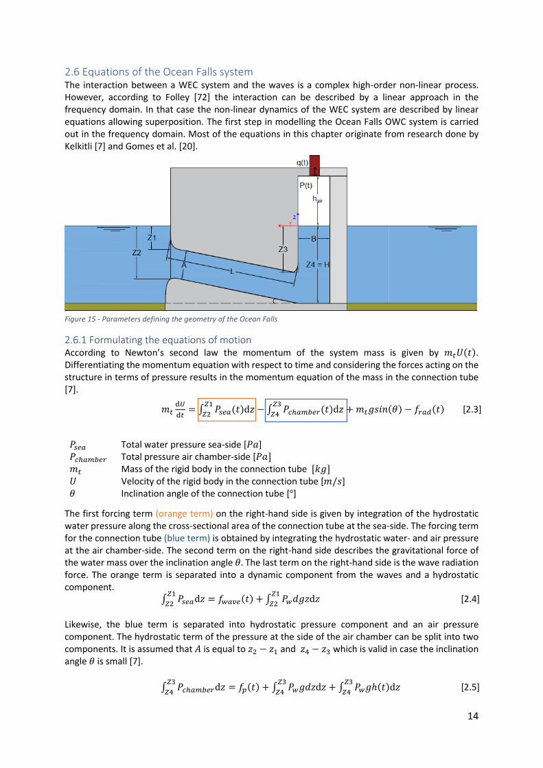
2.6 Equations of the Ocean Falls system The interaction between a WEC system and the waves is a complex high-order non-linear process. However, according to Folley [72] the interaction can be described by a linear approach in the frequency domain. In that case the non-linear dynamics of the WEC system are described by linear equations allowing superposition. The first step in modelling the Ocean Falls OWC system is carried out in the frequency domain. Most of the equations in this chapter originate from research done by Kelkitli [7] and Gomes et al. [20].

Figure 15 - Parameters defining the geometry of the Ocean Falls

2.6.1 Formulating the equations of motion According to Newton’s second law the momentum of the system mass is given by 𝑚𝑡𝑈(𝑡). Differentiating the momentum equation with respect to time and considering the forces acting on the structure in terms of pressure results in the momentum equation of the mass in the connection tube [7].

The first forcing term (orange term) on the right-hand side is given by integration of the hydrostatic water pressure along the cross-sectional area of the connection tube at the sea-side. The forcing term for the connection tube (blue term) is obtained by integrating the hydrostatic water- and air pressure at the air chamber-side. The second term on the right-hand side describes the gravitational force of the water mass over the inclination angle 휃. The last term on the right-hand side is the wave radiation force. The orange term is separated into a dynamic component from the waves and a hydrostatic component.

Likewise, the blue term is separated into hydrostatic pressure component and an air pressure component. The hydrostatic term of the pressure at the side of the air chamber can be split into two components. It is assumed that 𝐴 is equal to 𝑧2 − 𝑧1 and 𝑧4 − 𝑧3 which is valid in case the inclination angle 휃 is small [7].

𝑃𝑠𝑒𝑎 Total water pressure sea-side [𝑃𝑎] 𝑃𝑐ℎ𝑎𝑚𝑏𝑒𝑟 Total pressure air chamber-side [𝑃𝑎] 𝑚𝑡 Mass of the rigid body in the connection tube [𝑘𝑔] 𝑈 Velocity of the rigid body in the connection tube [𝑚/𝑠] 휃 Inclination angle of the connection tube [°]

15

𝑈(𝑡) =𝐵

𝐴ℎ(𝑡) [2.6]

[2.3]

[2.2]

𝜌𝑤𝐵ℎ(𝑡) +𝜌𝑤𝑔𝐴

𝐿ℎ(𝑡) +

𝐴

𝐿𝑝(𝑡) =

𝑓𝑤𝑎𝑣𝑒(𝑡)

d𝐿−

𝑓𝑟𝑎𝑑(𝑡)

d𝐿 [2.7]

[2.2]

For the Ocean Falls system, there is an oscillation of the rigid body in the connection tube and an oscillation of the water surface ℎ(𝑡) inside the air chamber. Both oscillations are coupled by applying the mass conservation law for incompressible fluid [7]. Dividing by 𝑑 makes the problem 2-dimensional. This results in the first equation of motion in the time domain for the oscillation of the internal water surface.

𝜌𝑤 Water density [𝑘𝑔/𝑚3] 𝐵 Width of the air chamber [𝑚] 𝐿 Length of the connection tube [𝑚] 𝐴 Height of the connection tube [𝑚] 𝑓𝑟𝑎𝑑 Wave radiation force [𝑁] 𝑝(𝑡) Air chamber pressure [𝑃𝑎] 𝑓𝑤𝑎𝑣𝑒 Wave forcing [𝑁]

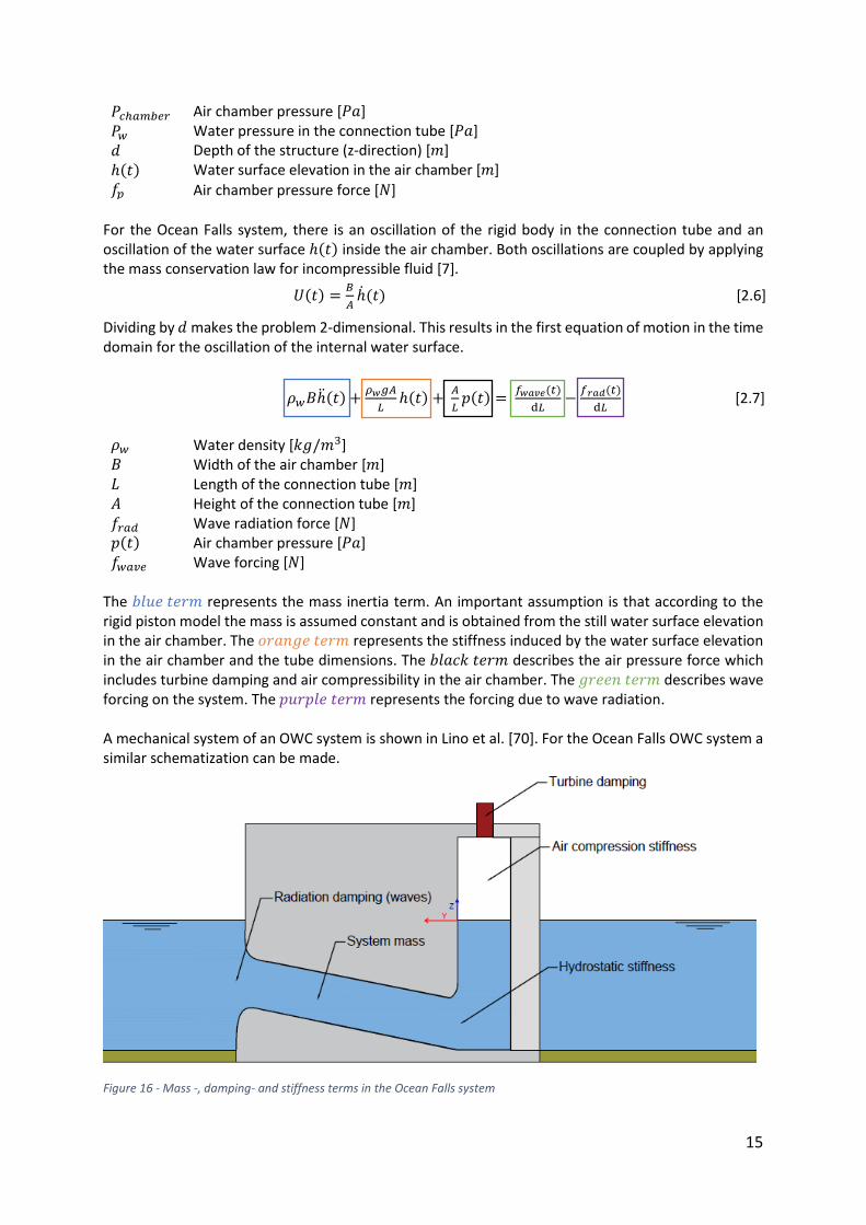
The 𝑏𝑙𝑢𝑒 𝑡𝑒𝑟𝑚 represents the mass inertia term. An important assumption is that according to the rigid piston model the mass is assumed constant and is obtained from the still water surface elevation in the air chamber. The 𝑜𝑟𝑎𝑛𝑔𝑒 𝑡𝑒𝑟𝑚 represents the stiffness induced by the water surface elevation in the air chamber and the tube dimensions. The 𝑏𝑙𝑎𝑐𝑘 𝑡𝑒𝑟𝑚 describes the air pressure force which includes turbine damping and air compressibility in the air chamber. The 𝑔𝑟𝑒𝑒𝑛 𝑡𝑒𝑟𝑚 describes wave forcing on the system. The 𝑝𝑢𝑟𝑝𝑙𝑒 𝑡𝑒𝑟𝑚 represents the forcing due to wave radiation. A mechanical system of an OWC system is shown in Lino et al. [70]. For the Ocean Falls OWC system a similar schematization can be made.

Figure 16 - Mass -, damping- and stiffness terms in the Ocean Falls system

𝑃𝑐ℎ𝑎𝑚𝑏𝑒𝑟 Air chamber pressure [𝑃𝑎] 𝑃𝑤 Water pressure in the connection tube [𝑃𝑎] 𝑑 Depth of the structure (z-direction) [𝑚] ℎ(𝑡) Water surface elevation in the air chamber [𝑚] 𝑓𝑝 Air chamber pressure force [𝑁]

16

Ψ = 𝑝

𝜌𝑎Ω2𝐷2 𝑎𝑛𝑑 Φ =��

𝜌𝑎Ω𝐷3 [2.9]

[2.2]

Φ = 𝐾Ψ [2.10]

[2.2]

𝐾𝑡𝑢𝑟𝑏𝑖𝑛𝑒𝑝(𝑡) = 𝜌𝑎𝐵ℎ(𝑡) −𝐵ℎ𝑎𝑖𝑟

𝑐2 ��(𝑡) [2.12]

[2.2]

𝑐2 =𝜌𝑎

𝛾𝑝𝑎 [2.13]

[2.2]

��(𝑡) = 𝜌𝑎𝐵𝑑ℎ(𝑡) −𝜌𝑎𝐵𝑑ℎ𝑎𝑖𝑟

𝛾𝜌𝑎��(𝑡) [2.8]

[2.2]

The radiation damping and the system mass are frequency dependent. In the parametric model each individual frequency in the wave spectrum is characterized by unique values of mass and damping. The relation between the pressure and water surface elevation in the air chamber is obtained from Sheng et al. [63] and Gomes et al. [10].

𝜌𝑎 Atmospheric air density [𝑘𝑔/𝑚3] 𝛾 Specific heat ratio of air [−] ℎ𝑎𝑖𝑟 Height above the water surface in the air chamber [𝑚]

Note that eq. 2.8 originates from the conservation of mass inside the air chamber while considering an ideal gas and the air compressibility inside the chamber as an isentropic process.

2.6.2 Linear turbine For the Ocean Falls OWC system a self-rectifying turbine is applied meaning that the torque is not sensitive to the air flow direction. This type of turbine can convert a flow in two directions into an uni-directional flow. Two types of air turbines which are commonly applied for OWC systems are the Wells turbine invented by A.A. Wells in the late 1970 and the bi-radial impulse turbine. According to Falcao [34] the latter is the most frequently proposed and applied air turbine for OWC systems. Additional information about these turbines is provided in chapter A.3.6 in the appendix. In chapter 3.8 it is decided which type of turbine is considered for this research. The relation between the air chamber pressure and the mass flow through the turbine is obtained by applying the theory of Dixon [11].

Ω Angular velocity [𝑟𝑎𝑑/𝑠] 𝐷 Turbine diameter [𝑚] Φ Dimensionless flow rate [−] Ψ Dimensionless pressure ratio [−]

As described by Dixon [11] the relation between the airflow and the pressure is assumed linear.

𝐾 Dimensionless turbine proportionality constant [−] The mass flow through the turbine can be expressed as follows:

The turbine coefficient

𝐾𝐷

Ω is for simplicity from now on denoted as 𝑘𝑡𝑢𝑟𝑏𝑖𝑛𝑒. Because the parametric

model is 2D 𝑘𝑡𝑢𝑟𝑏𝑖𝑛𝑒 is divided by the width of the structure 𝐵𝑠𝑦𝑠𝑡𝑒𝑚 in x-direction. Combining

equations 2.8 and 2.11 results in the equation describing the mass flow through the turbine.

𝑐 Speed of sound [𝑚/𝑠] 𝛾 Adiabatic constant [−]

��(t) =𝐾𝐷

Ω𝑝(𝑡) [2.11]

[2.2]

17

��(t) = 𝐾𝑡𝑢𝑟𝑏𝑖𝑛𝑒𝑝(𝑡) = 𝜌𝑎𝐵ℎ(𝑡) −𝐵ℎ𝑎𝑖𝑟

𝑐2 ��(𝑡) [2.15]

[2.2]

𝑃𝑡(t) =��(𝑡)

ρa𝑝(𝑡) =

𝐾𝑡𝑢𝑟𝑏𝑖𝑛𝑒

𝜌𝑎𝑝(𝑡)2 [2.16]

[2.2]

��𝑟𝑎𝑑 = −𝜔2𝐴(𝜔)�� + 𝑖𝜔𝐵(𝜔)�� [2.17]

[2.2]

�� =��(𝜔)

−𝜔2(𝜌𝑤𝐵+𝑚𝑎(𝜔)

𝐿)+𝑖𝜔(

𝐵𝑟(𝜔)

𝐿+

𝐵𝐴

𝐿Λ)+

𝜌𝑤𝑔𝐴

𝐿

= ��(𝜔)

−𝜔2(𝑚)+𝑖𝜔(𝑏𝑒𝑓𝑓)+𝑘𝑒𝑓𝑓 [2.18]

[2.2]

�� = Λ�� = 𝑖𝜔Λ𝐵�� [2.19]

[2.2]

Λ = (𝐾𝑡𝑢𝑟𝑏𝑖𝑛𝑒

𝜌𝑎+

𝑖𝜔𝐵ℎ𝑎𝑖𝑟

𝜌𝑎𝑐2 )−1

[2.20]

[2.2]

𝑃�� =𝐾𝑡𝑢𝑟𝑏𝑖𝑛𝑒

2𝜌𝑎|��|

2 [2.22]

[2.2]

��(𝜔) =𝐴𝑖𝑛𝑐𝐹𝑤𝑎𝑣𝑒(𝜔)

𝐿 [2.21]

[2.2]

𝜌𝑤𝐵ℎ(𝑡) +𝜌𝑤𝑔𝐴

𝐿ℎ(𝑡) +

𝐴

𝐿𝑝(𝑡) =

𝑓𝑤𝑎𝑣𝑒(𝑡)

d𝐿−

𝑓𝑟𝑎𝑑(𝑡)

d𝐿 [2.14]

The terms on the right-hand side of eq. 2.12 are both linearized. Now two linearized coupled equations of motion can be formulated [7]. The first equation describes the oscillation of the water surface whereas the second equation describes the mass flow through the turbine. The power available to the power take-off system (PTO) is defined as:

2.6.3 Radiation forcing Due to the oscillating of the water surface elevation inside the air chamber the water mass will accelerate/decelerate creating radiation waves which remove energy from the system. The radiation forcing is defined in the frequency domain [7] and is based on linear wave theory [4].

𝐴(𝜔) Frequency dependent added mass [𝑘𝑔] 𝐵(𝜔) Frequency dependent radiation damping [𝑁𝑠/𝑚]

�� Complex amplitude of the water surface elevation in the air chamber [−] 𝜔 Frequency of the oscillating mass [𝑟𝑎𝑑/𝑠]

For this research the calculation of the hydrodynamic coefficients; added mass, radiation damping, diffraction and Froude-Krylov forcing is done with numerical diffraction software ANSYS AQWA.

2.6.4 Solutions in the frequency domain Both equation 2.14 and 2.15 are solved in the frequency domain by Kelkitli [7] to obtain the complex

amplitudes of water surface elevation �� and pressure �� in the air chamber.

𝐵𝑟(𝜔) = 𝐵(𝜔) Frequency dependent radiation damping [𝑁𝑠/𝑚] 𝐹𝑤𝑎𝑣𝑒(𝜔) Wave excitation from diffraction and Froude-Krylov forcing [𝑁/𝑚] 𝐴𝑖𝑛𝑐 Incoming wave amplitude [𝑚]

Following the method described in Gomes et al. [10] the time averaged power available to the PTO system over one wave period is defined as:

18

beff =𝐵𝑟(𝜔)

𝐿+

(𝐵𝐴

𝐿)(

𝐾𝑡𝑢𝑟𝑏𝑖𝑛𝑒𝜌𝑎

)

(𝐾𝑡𝑢𝑟𝑏𝑖𝑛𝑒

𝜌𝑎)

2+𝜔2(

𝐵ℎ𝑎𝑖𝑟𝜌𝑎𝑐2 )

2 [2.24]

𝜔eff = 𝜔0√1 − 휁𝑒𝑓𝑓(𝜔)2 [2.25]

[2.2]

휁𝑒𝑓𝑓 =𝑏𝑒𝑓𝑓(𝜔)

2√𝑘𝑒𝑓𝑓(𝜔)𝑚(𝜔) [2.26]

[2.2]

𝜔0 = √𝑘𝑒𝑓𝑓(𝜔)

𝑚(𝜔) [2.27]

[2.2]

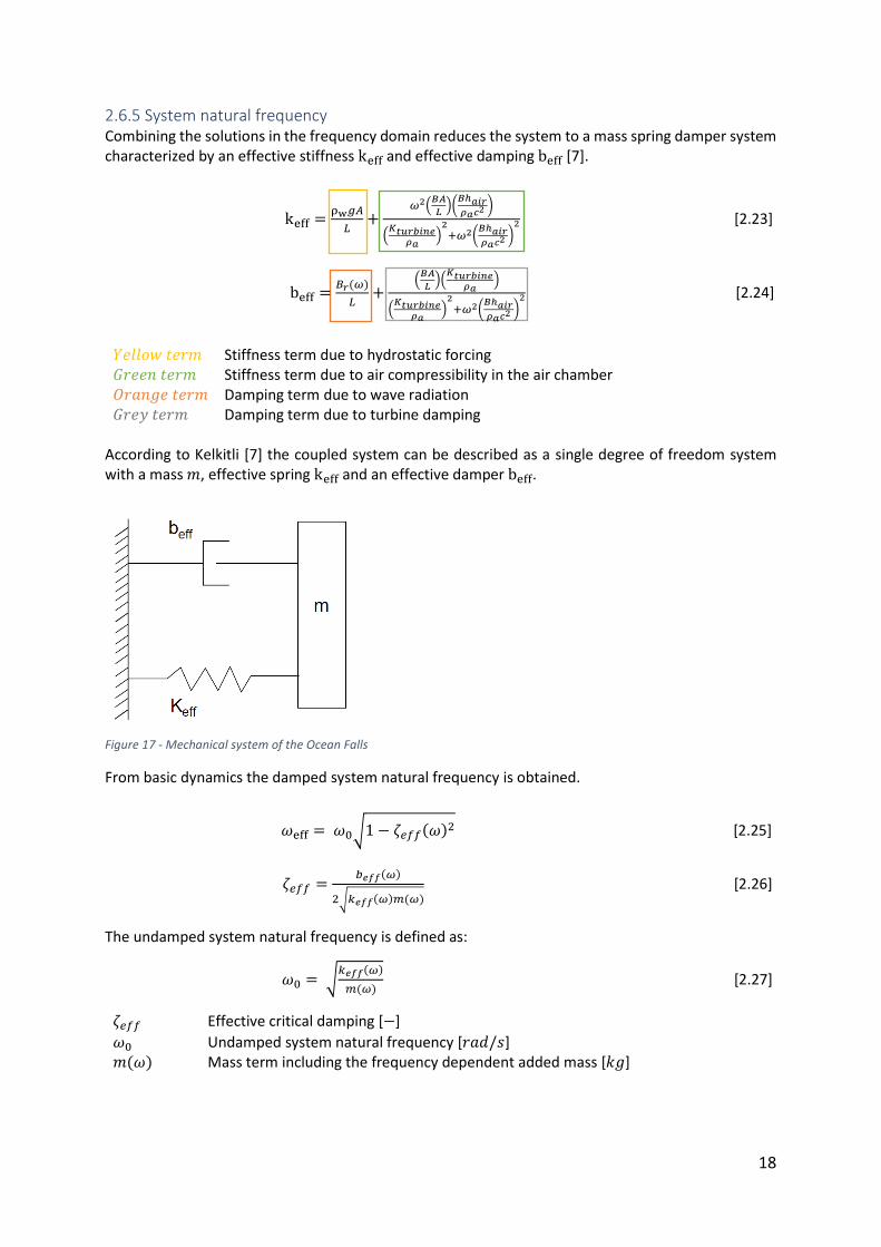
2.6.5 System natural frequency Combining the solutions in the frequency domain reduces the system to a mass spring damper system characterized by an effective stiffness keff and effective damping beff [7].

According to Kelkitli [7] the coupled system can be described as a single degree of freedom system with a mass 𝑚, effective spring keff and an effective damper beff.

Figure 17 - Mechanical system of the Ocean Falls

From basic dynamics the damped system natural frequency is obtained.

The undamped system natural frequency is defined as:

휁𝑒𝑓𝑓 Effective critical damping [−]

𝜔0 Undamped system natural frequency [𝑟𝑎𝑑/𝑠] 𝑚(𝜔) Mass term including the frequency dependent added mass [𝑘𝑔]

𝑌𝑒𝑙𝑙𝑜𝑤 𝑡𝑒𝑟𝑚 Stiffness term due to hydrostatic forcing 𝐺𝑟𝑒𝑒𝑛 𝑡𝑒𝑟𝑚 Stiffness term due to air compressibility in the air chamber 𝑂𝑟𝑎𝑛𝑔𝑒 𝑡𝑒𝑟𝑚 Damping term due to wave radiation 𝐺𝑟𝑒𝑦 𝑡𝑒𝑟𝑚 Damping term due to turbine damping

keff =ρw𝑔𝐴

𝐿+

𝜔2(𝐵𝐴

𝐿)(

𝐵ℎ𝑎𝑖𝑟𝜌𝑎𝑐2 )

(𝐾𝑡𝑢𝑟𝑏𝑖𝑛𝑒

𝜌𝑎)

2+𝜔2(

𝐵ℎ𝑎𝑖𝑟𝜌𝑎𝑐2 )

2 [2.23]

19

𝑓𝑝𝑑𝑓(휁) =1

√2𝜋𝜎𝜁exp (−

𝜁2

2𝜎𝜁2) [2.28]

[2.2]

𝜎𝜁2 = ∫ 𝑆ω

∞

0(𝜔)d𝜔 [2.29]

[2.2]

𝜎𝑝2 = ∫ 𝑆ω

∞

0(𝜔)|

��(𝜔)

𝜁𝑎|2d𝜔 [2.32]

[2.2]

2.6.6 Power obtained from irregular waves Because linear wave theory is applied and it is assumed that all waves are traveling in the same direction; irregular waves are considered as a linear superposition of multiple sinusoidal regular waves [4]. According to Gomes et al. [20] the free-surface can be described by a Gaussian probability density function.

휁 Free surface elevation [𝑚] 𝜎𝜁 Standard deviation [𝑚]

Once the standard deviation of the spectrum is known, the variance of the spectrum can be calculated.

𝑆ω(ω) Energy density spectrum of the irregular sea state [𝑚2/𝑟𝑎𝑑/𝑠] 𝜔 Wave excitation frequency [𝑟𝑎𝑑/𝑠]

The energy density spectrum can be described by a Pierson-Moskowitz or a JONSWAP wave spectrum. For this research the JONSWAP energy density spectrum 𝑆ω(𝜔) is applied including the peak wave period 𝑇𝑝 as described by Hasselman [12].

𝐻𝑠 Significant wave height [𝑚] 𝑇𝑝 Peak wave period [𝑠]

𝛾 Peakedness factor [−]

With the JONSWAP irregular wave spectrum, the response of the system elevation and pressure can be described in terms of spectral density. The standard deviation of the water surface elevation 𝜎ℎ and the pressure difference 𝜎𝑝 for irregular waves are obtained from Gomes et al. [20]. These expressions

include the complex amplitudes for elevation �� and pressure �� in the air chamber of the OWC.

휁𝑎 Wave amplitude [𝑚]

�� Complex amplitude of the water surface elevation in the air chamber [𝑚]

�� Complex amplitude of the air chamber pressure [𝑃𝑎]

According to Gomes et al. [20] the time-averaged power available to the PTO system from irregular waves is defined as:

𝑆ω(𝜔) =320𝐻𝑠

2

𝑇𝑝4 ω−5 exp (−

−1950

𝑇𝑝4 𝜔−4) 𝛾𝛼(𝜔) [2.30]

[2.2]

𝜎ℎ2 = ∫ 𝑆ω

∞

0(𝜔)|

��(𝜔)

𝜁𝑎|2d𝜔 [2.31]

[2.2]

��𝑡,𝑖𝑟𝑟𝑒𝑔𝑢𝑙𝑎𝑟 =𝐾𝑡𝑢𝑟𝑏𝑖𝑛𝑒

ρa𝜎𝑝

2

[2.33]

[2.2]

20

𝐽��𝑟𝑟𝑒𝑔𝑢𝑙𝑎𝑟 = ∑ 𝐽(휁𝑎(𝜔)) [2.36]

[2.2]

휁𝑎(𝜔) = √2𝑆𝜔(𝜔)d𝜔 [2.37]

[2.2]

𝐿𝑐 =��𝑡,𝑖𝑟𝑟𝑒𝑔𝑢𝑙𝑎𝑟

𝐽��𝑟𝑟𝑒𝑔𝑢𝑙𝑎𝑟 [2.38]

[2.2]

휂 =��𝑡,𝑖𝑟𝑟𝑒𝑔𝑢𝑙𝑎𝑟

𝐽��𝑟𝑟𝑒𝑔𝑢𝑙𝑎𝑟𝐵𝑠𝑦𝑠𝑡𝑒𝑚 [2.39]

[2.2]

𝐽��𝑒𝑔𝑢𝑙𝑎𝑟 =1

2𝜌𝑤𝑔휁𝑎

2𝑐𝑔 [2.34]

[2.2]

𝑐𝑔 =𝜔

2𝑘(1 + (

2𝑘𝑑

sinh(2𝑘𝑑))) [2.35]

[2.2]

2.6.7 System efficiency The overall efficiency of the conversion from wave to wire consists of the efficiency of the OWC system, the efficiency of the turbine and the efficiency of the generator (Figure A.3.35). In this research only the efficiency of the OWC system is considered. Therefore, the system efficiency is defined as the power available to the power take-off system (PTO) divided by the available wave energy flux. As explained in Holthuijsen [64] the wave energy flux for regular waves is defined as:

휁𝑎(𝜔) Incoming wave amplitude of a single regular wave [𝑚] 𝐽 Wave energy flux per meter wave crest [𝑊/𝑚] 𝑐𝑔 Group velocity of the waves in intermediate water depth [𝑚/𝑠]

𝑑 Water depth [𝑚] 𝑘 Wave number [𝑚−1]

Locally there are multiple wave directions. However, since in this research a 2D parametric model is applied single-directional waves are considered. The time-averaged wave energy flux for irregular waves equals the sum of wave energy fluxes from the regular waves in the spectrum as explained by Gomez et al. [20].

𝑑𝜔 Frequency interval [𝑟𝑎𝑑/𝑠] The ratio between the power available to the power take-off system and the available wave energy flux is described in terms of the capture width 𝐿𝑐. The system efficiency is obtained by dividing the capture width over the width of the system 𝐵𝑠𝑦𝑠𝑡𝑒𝑚.

21

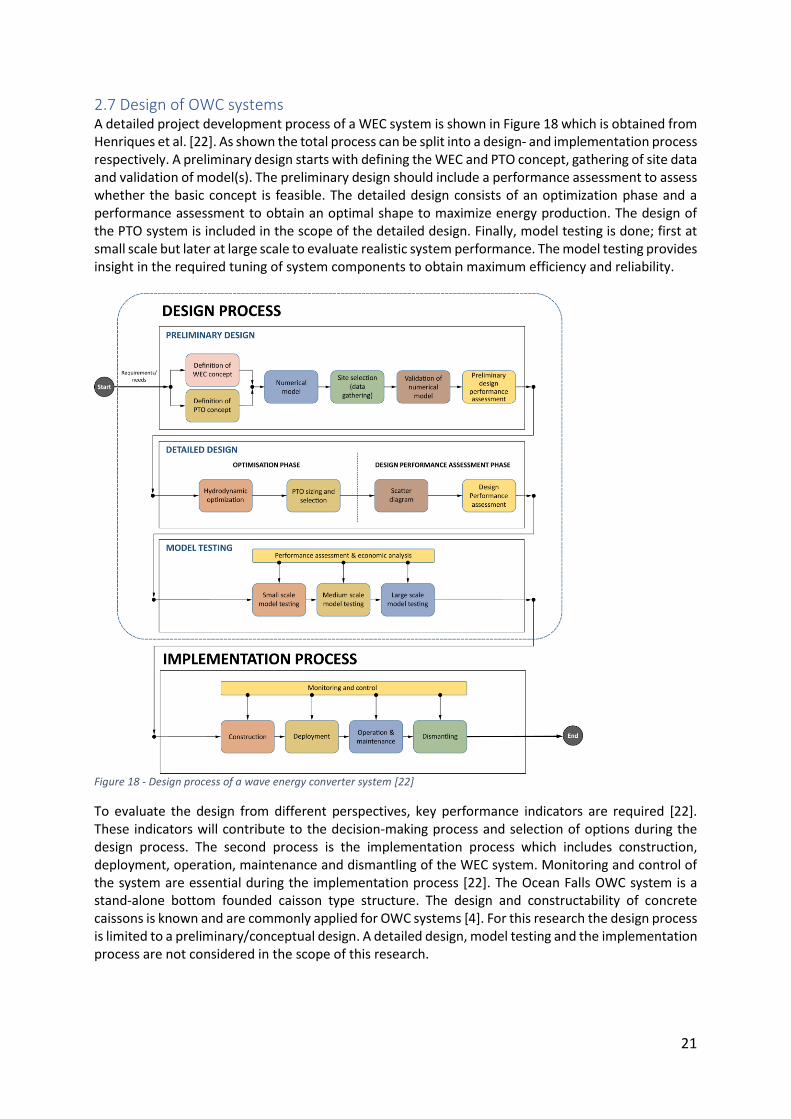
2.7 Design of OWC systems A detailed project development process of a WEC system is shown in Figure 18 which is obtained from Henriques et al. [22]. As shown the total process can be split into a design- and implementation process respectively. A preliminary design starts with defining the WEC and PTO concept, gathering of site data and validation of model(s). The preliminary design should include a performance assessment to assess whether the basic concept is feasible. The detailed design consists of an optimization phase and a performance assessment to obtain an optimal shape to maximize energy production. The design of the PTO system is included in the scope of the detailed design. Finally, model testing is done; first at small scale but later at large scale to evaluate realistic system performance. The model testing provides insight in the required tuning of system components to obtain maximum efficiency and reliability.

Figure 18 - Design process of a wave energy converter system [22]

To evaluate the design from different perspectives, key performance indicators are required [22]. These indicators will contribute to the decision-making process and selection of options during the design process. The second process is the implementation process which includes construction, deployment, operation, maintenance and dismantling of the WEC system. Monitoring and control of the system are essential during the implementation process [22]. The Ocean Falls OWC system is a stand-alone bottom founded caisson type structure. The design and constructability of concrete caissons is known and are commonly applied for OWC systems [4]. For this research the design process is limited to a preliminary/conceptual design. A detailed design, model testing and the implementation process are not considered in the scope of this research.

22

3 Performance assessment of the Ocean falls

3.1 Introduction and chapter outline In this chapter a performance assessment of the Ocean Falls is done. The term system performance will be repeated many times in this chapter and represents the system efficiency. System efficiency: The power available to the power take-off system (PTO) divided by the available wave energy flux. A high system performance resembles a high system efficiency (휂) and much energy available to the PTO (𝑃��). Note that the efficiencies of the turbine and the generator are not considered in the scope of this research. For this research two models are applied: 1 - Parametric model (ANSYS AQWA and Python): Numerical frequency domain model which calculates the system performance in terms of power to the PTO and system efficiency. A Python script includes all differential equations required to model the Ocean Falls OWC system. Numerical diffraction software ANSYS AQWA is applied to calculate the hydrodynamic coefficients; added mass, radiation damping, diffraction and Froude-Krylov forcing in the frequency domain. 2 - CFD model (ANSYS Fluent): ANSYS Fluent software is applied for numerical modelling of the OWC system. The model provides insight in the system behavior, considers non-linear hydrodynamic effects and can simulate complex flow interaction. Further information about the model is provided in chapter A.3.7.1. Section 3.2 and 3.3 elaborate on the parametric model distinguishing the analytical (Python) part and the ANSYS AQWA model. Section 3.4 elaborates on the influence of the piston position on the results obtained from the ANSYS AQWA model. In section 3.5 the influence of the hydrodynamic coefficients is observed and explained. In section 3.6 the influence of geometry on the system response is observed and explained. Section 3.7 elaborates on the system performance for a regular- and irregular sea-state. Section 3.8 elaborates on the system performance of the Ocean Falls for different geometries. Section 3.9 elaborates on the CFD model applied for this research. Finally, in section 3.10 a decision on a design is made based on three criteria: system performance, constructability and cost effectiveness.

3.2 Parametric model - Python

3.2.1 Objective The objective of this section is to elaborate on the analytical (Python) part of the parametric model. This part includes all system equations shown in section 2.6 of which the script is shown in chapter A.5. in the appendix. In this section the limitations of the model with respect to reality are discussed.

3.2.2 Method The model includes the system equations shown in section 2.6 which are required to calculate the power output and system efficiency. In the model the Ocean Falls system is considered as a single degree of freedom mass-spring-damper system as shown in Figure 17. The rigid body represents the mass, the hydrostatic stiffness represents the spring and the air compressibility, radiation- and turbine damping represent the damper. The frequency domain model applies the frequency dependent hydrodynamic coefficients obtained from ANSYS AQWA to calculate the system performance. The model calculates the system performance for each respective frequency considering either regular- or irregular waves.

23

3.2.3 Results In this section several assumptions and limitations of the parametric model are discussed.

I. Ideal gas laws: The model assumes that no heat and matter is transferred and neglects this loss of energy.

II. Linear wave theory: The model assumes the water to be incompressible and irrotational and includes the assumptions made in linear wave theory. These assumptions are discussed in chapter A.1.1 in the appendix.

III. Horizontal flat surface: The model is based on the rigid piston approach which assumes that the water surface in the air chamber remains horizontal.

IV. Uniform pressure: The pressure inside the air chamber is assumed to be uniform and there are

no changes is pressure intensity on a certain moment in time.

V. Linear model: The model assumes a linear relation between pressure and airflow through the turbine. Meaning that the volume of air in the chamber does not depend on the internal water surface elevation and ℎ𝑎𝑖𝑟 >> 𝑧 (Figure 25). Model scale experiments by Kelkitli [7] and Falcao [34] have shown that this relation is non-linear since the pressure-flow relation is quadratic. The air compressibility has a small effect in case of model scale devices but is generally important for full-scale devices according to Bingham [42]. To include the effect of non-linear air compressibility a non-linear analysis should be done with e.g. a CFD model.

VI. Irregular wave damping: Once the irregular waves enter the system, the waves start to interact. The wave interaction results in damping of the waves in the system which is not accounted for in the model. This results in an underestimation of the system damping with respect to reality.

3.3 Parametric model - ANSYS AQWA

3.3.1 Objective The objective of this section is to elaborate on the ANSYS AQWA part of the parametric model. This section elaborates on how the model is made and the limitations of the model with respect to reality.

3.3.2 Method Numerical diffraction software ANSYS AQWA is applied to calculate the hydrodynamic coefficients; added mass, radiation damping, diffraction and Froude-Krylov forcing in the frequency domain. A parametrical design model is developed in ANSYS Design Modeler to configure different geometries. Information about the solution method and the ANSYS AQWA model applied for this research is provided in the appendix chapter A.3.1. In total two bodies can be distinguished:

I. Outer body: This body is fixed in place and consists of the inlet, connection tube, air chamber and walls around the structure. The panels of the outer body are all diffracting.

II. Piston: Because the numerical diffraction software ANSYS AQWA is unable to characterize a (oscillating) mass in the connection tube a piston is modelled. The piston oscillates in horizontal x-direction and resembles the rigid body inside the connection tube. The incoming waves induce an oscillation of the piston which causes the two bodies to interact. Because the piston does not exist in reality; the panel of the piston is non-diffracting.

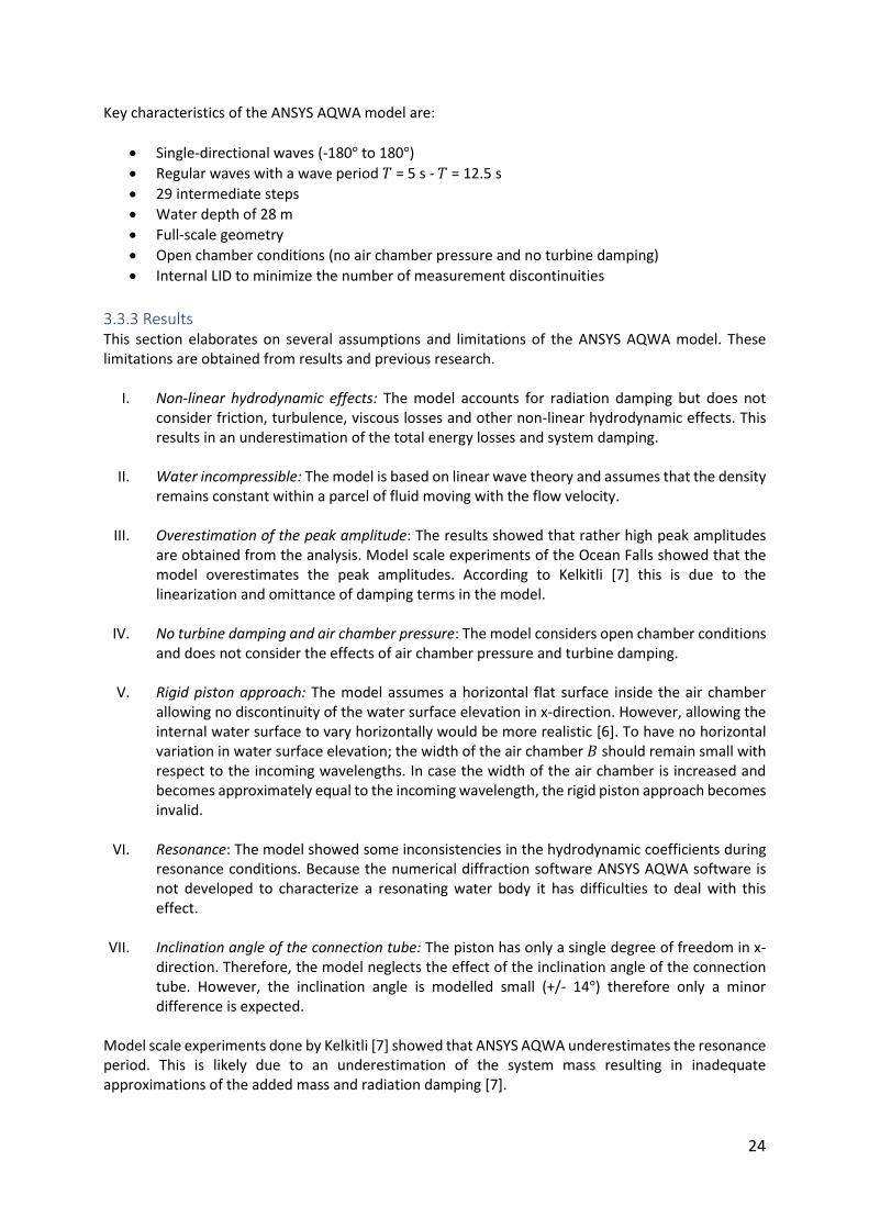
24

Key characteristics of the ANSYS AQWA model are:

• Single-directional waves (-180° to 180°)

• Regular waves with a wave period 𝑇 = 5 s - 𝑇 = 12.5 s

• 29 intermediate steps

• Water depth of 28 m

• Full-scale geometry

• Open chamber conditions (no air chamber pressure and no turbine damping)

• Internal LID to minimize the number of measurement discontinuities

3.3.3 Results This section elaborates on several assumptions and limitations of the ANSYS AQWA model. These limitations are obtained from results and previous research.

I. Non-linear hydrodynamic effects: The model accounts for radiation damping but does not consider friction, turbulence, viscous losses and other non-linear hydrodynamic effects. This results in an underestimation of the total energy losses and system damping.

II. Water incompressible: The model is based on linear wave theory and assumes that the density

remains constant within a parcel of fluid moving with the flow velocity.

III. Overestimation of the peak amplitude: The results showed that rather high peak amplitudes are obtained from the analysis. Model scale experiments of the Ocean Falls showed that the model overestimates the peak amplitudes. According to Kelkitli [7] this is due to the linearization and omittance of damping terms in the model.

IV. No turbine damping and air chamber pressure: The model considers open chamber conditions

and does not consider the effects of air chamber pressure and turbine damping.

V. Rigid piston approach: The model assumes a horizontal flat surface inside the air chamber allowing no discontinuity of the water surface elevation in x-direction. However, allowing the internal water surface to vary horizontally would be more realistic [6]. To have no horizontal variation in water surface elevation; the width of the air chamber 𝐵 should remain small with respect to the incoming wavelengths. In case the width of the air chamber is increased and becomes approximately equal to the incoming wavelength, the rigid piston approach becomes invalid.

VI. Resonance: The model showed some inconsistencies in the hydrodynamic coefficients during

resonance conditions. Because the numerical diffraction software ANSYS AQWA software is not developed to characterize a resonating water body it has difficulties to deal with this effect.

VII. Inclination angle of the connection tube: The piston has only a single degree of freedom in x-

direction. Therefore, the model neglects the effect of the inclination angle of the connection tube. However, the inclination angle is modelled small (+/- 14°) therefore only a minor difference is expected.

Model scale experiments done by Kelkitli [7] showed that ANSYS AQWA underestimates the resonance period. This is likely due to an underestimation of the system mass resulting in inadequate approximations of the added mass and radiation damping [7].

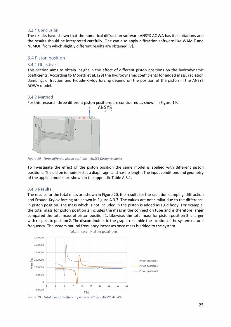
25

3.3.4 Conclusion The results have shown that the numerical diffraction software ANSYS AQWA has its limitations and the results should be interpreted carefully. One can also apply diffraction software like WAMIT and NEMOH from which slightly different results are obtained [7].

3.4 Piston position

3.4.1 Objective This section aims to obtain insight in the effect of different piston positions on the hydrodynamic coefficients. According to Moretti et al. [29] the hydrodynamic coefficients for added mass, radiation damping, diffraction and Froude-Krylov forcing depend on the position of the piston in the ANSYS AQWA model.

3.4.2 Method For this research three different piston positions are considered as shown in Figure 19.

Figure 19 - Three different piston positions - ANSYS Design Modeler

To investigate the effect of the piston position the same model is applied with different piston positions. The piston is modelled as a diaphragm and has no length. The input conditions and geometry of the applied model are shown in the appendix Table A.3.1.

3.4.3 Results The results for the total mass are shown in Figure 20, the results for the radiation damping, diffraction and Froude-Krylov forcing are shown in Figure A.3.7. The values are not similar due to the difference in piston position. The mass which is not included in the piston is added as rigid body. For example, the total mass for piston position 2 includes the mass in the connection tube and is therefore larger compared the total mass of piston position 1. Likewise, the total mass for piston position 3 is larger with respect to position 2. The discontinuities in the graphs resemble the location of the system natural frequency. The system natural frequency increases once mass is added to the system.

Figure 20 - Total mass for different piston positions - ANSYS AQWA

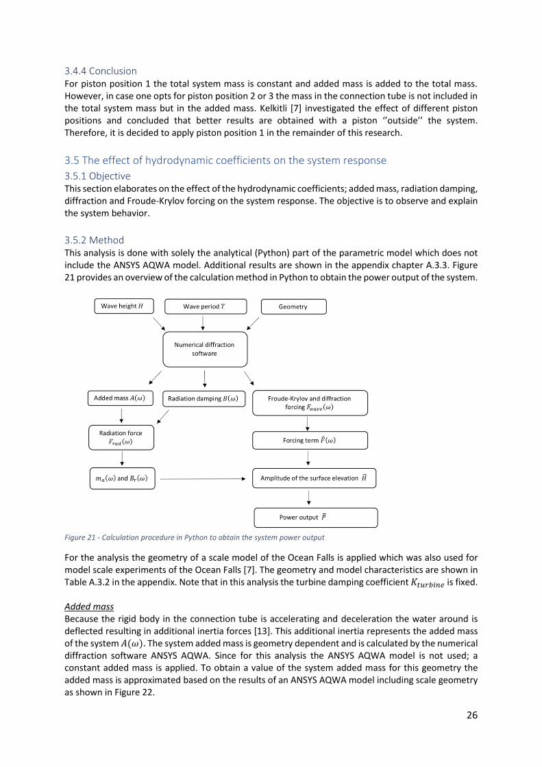
26

3.4.4 Conclusion For piston position 1 the total system mass is constant and added mass is added to the total mass. However, in case one opts for piston position 2 or 3 the mass in the connection tube is not included in the total system mass but in the added mass. Kelkitli [7] investigated the effect of different piston positions and concluded that better results are obtained with a piston ‘’outside’’ the system. Therefore, it is decided to apply piston position 1 in the remainder of this research.

3.5 The effect of hydrodynamic coefficients on the system response

3.5.1 Objective This section elaborates on the effect of the hydrodynamic coefficients; added mass, radiation damping, diffraction and Froude-Krylov forcing on the system response. The objective is to observe and explain the system behavior.

3.5.2 Method This analysis is done with solely the analytical (Python) part of the parametric model which does not include the ANSYS AQWA model. Additional results are shown in the appendix chapter A.3.3. Figure 21 provides an overview of the calculation method in Python to obtain the power output of the system.

Figure 21 - Calculation procedure in Python to obtain the system power output

For the analysis the geometry of a scale model of the Ocean Falls is applied which was also used for model scale experiments of the Ocean Falls [7]. The geometry and model characteristics are shown in Table A.3.2 in the appendix. Note that in this analysis the turbine damping coefficient 𝐾𝑡𝑢𝑟𝑏𝑖𝑛𝑒 is fixed. Added mass Because the rigid body in the connection tube is accelerating and deceleration the water around is deflected resulting in additional inertia forces [13]. This additional inertia represents the added mass of the system 𝐴(𝜔). The system added mass is geometry dependent and is calculated by the numerical diffraction software ANSYS AQWA. Since for this analysis the ANSYS AQWA model is not used; a constant added mass is applied. To obtain a value of the system added mass for this geometry the added mass is approximated based on the results of an ANSYS AQWA model including scale geometry as shown in Figure 22.

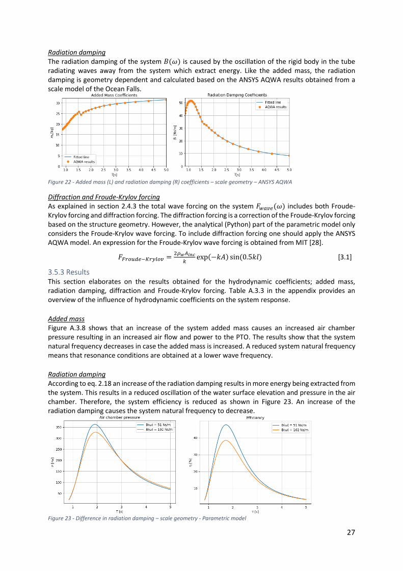
27

𝐹𝐹𝑟𝑜𝑢𝑑𝑒−𝐾𝑟𝑦𝑙𝑜𝑣 =2𝜌𝑤𝐴𝑖𝑛𝑐

𝑘exp(−𝑘𝐴) sin (0.5𝑘𝑙) [3.1]

[2.2]

Radiation damping The radiation damping of the system 𝐵(𝜔) is caused by the oscillation of the rigid body in the tube radiating waves away from the system which extract energy. Like the added mass, the radiation damping is geometry dependent and calculated based on the ANSYS AQWA results obtained from a scale model of the Ocean Falls.

Figure 22 - Added mass (L) and radiation damping (R) coefficients – scale geometry – ANSYS AQWA

Diffraction and Froude-Krylov forcing As explained in section 2.4.3 the total wave forcing on the system 𝐹𝑤𝑎𝑣𝑒(𝜔) includes both Froude-Krylov forcing and diffraction forcing. The diffraction forcing is a correction of the Froude-Krylov forcing based on the structure geometry. However, the analytical (Python) part of the parametric model only considers the Froude-Krylov wave forcing. To include diffraction forcing one should apply the ANSYS AQWA model. An expression for the Froude-Krylov wave forcing is obtained from MIT [28].

3.5.3 Results This section elaborates on the results obtained for the hydrodynamic coefficients; added mass, radiation damping, diffraction and Froude-Krylov forcing. Table A.3.3 in the appendix provides an overview of the influence of hydrodynamic coefficients on the system response.

Added mass Figure A.3.8 shows that an increase of the system added mass causes an increased air chamber pressure resulting in an increased air flow and power to the PTO. The results show that the system natural frequency decreases in case the added mass is increased. A reduced system natural frequency means that resonance conditions are obtained at a lower wave frequency.

Radiation damping According to eq. 2.18 an increase of the radiation damping results in more energy being extracted from the system. This results in a reduced oscillation of the water surface elevation and pressure in the air chamber. Therefore, the system efficiency is reduced as shown in Figure 23. An increase of the radiation damping causes the system natural frequency to decrease.

Figure 23 - Difference in radiation damping – scale geometry - Parametric model

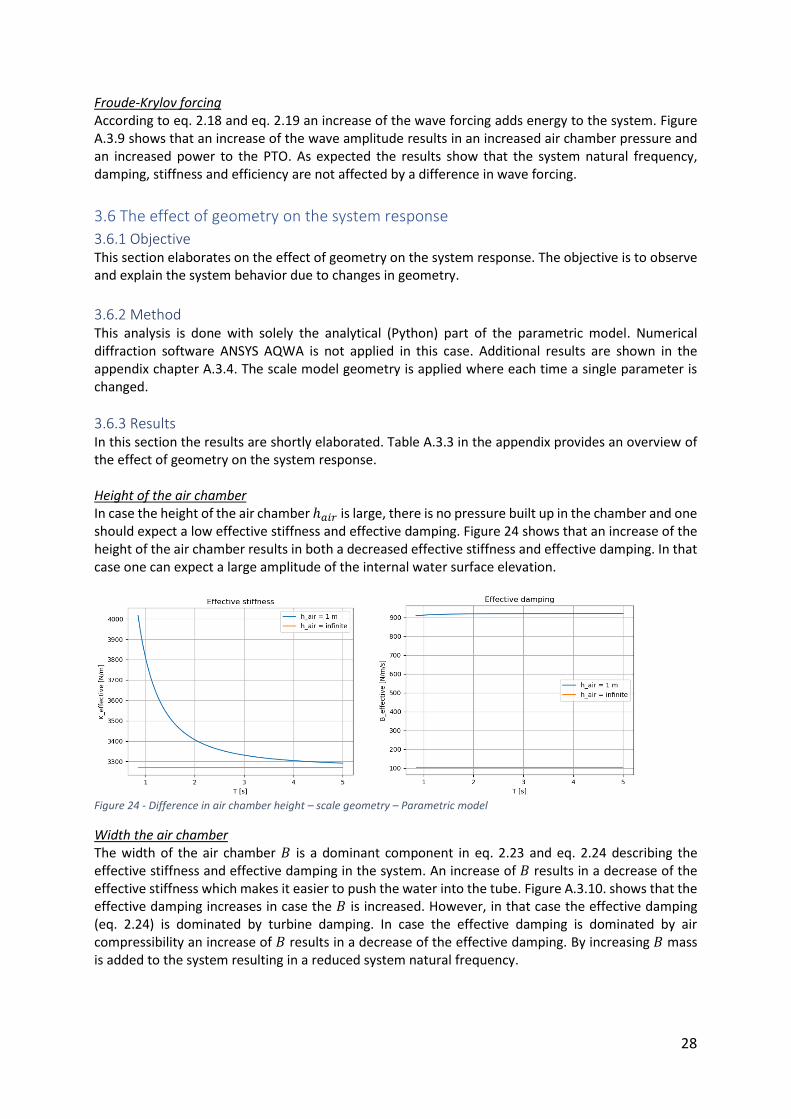
28

Froude-Krylov forcing According to eq. 2.18 and eq. 2.19 an increase of the wave forcing adds energy to the system. Figure A.3.9 shows that an increase of the wave amplitude results in an increased air chamber pressure and an increased power to the PTO. As expected the results show that the system natural frequency, damping, stiffness and efficiency are not affected by a difference in wave forcing.

3.6 The effect of geometry on the system response

3.6.1 Objective This section elaborates on the effect of geometry on the system response. The objective is to observe and explain the system behavior due to changes in geometry.

3.6.2 Method This analysis is done with solely the analytical (Python) part of the parametric model. Numerical diffraction software ANSYS AQWA is not applied in this case. Additional results are shown in the appendix chapter A.3.4. The scale model geometry is applied where each time a single parameter is changed.

3.6.3 Results In this section the results are shortly elaborated. Table A.3.3 in the appendix provides an overview of the effect of geometry on the system response. Height of the air chamber In case the height of the air chamber ℎ𝑎𝑖𝑟 is large, there is no pressure built up in the chamber and one should expect a low effective stiffness and effective damping. Figure 24 shows that an increase of the height of the air chamber results in both a decreased effective stiffness and effective damping. In that case one can expect a large amplitude of the internal water surface elevation.

Figure 24 - Difference in air chamber height – scale geometry – Parametric model

Width the air chamber The width of the air chamber 𝐵 is a dominant component in eq. 2.23 and eq. 2.24 describing the effective stiffness and effective damping in the system. An increase of 𝐵 results in a decrease of the effective stiffness which makes it easier to push the water into the tube. Figure A.3.10. shows that the effective damping increases in case the 𝐵 is increased. However, in that case the effective damping (eq. 2.24) is dominated by turbine damping. In case the effective damping is dominated by air compressibility an increase of 𝐵 results in a decrease of the effective damping. By increasing 𝐵 mass is added to the system resulting in a reduced system natural frequency.

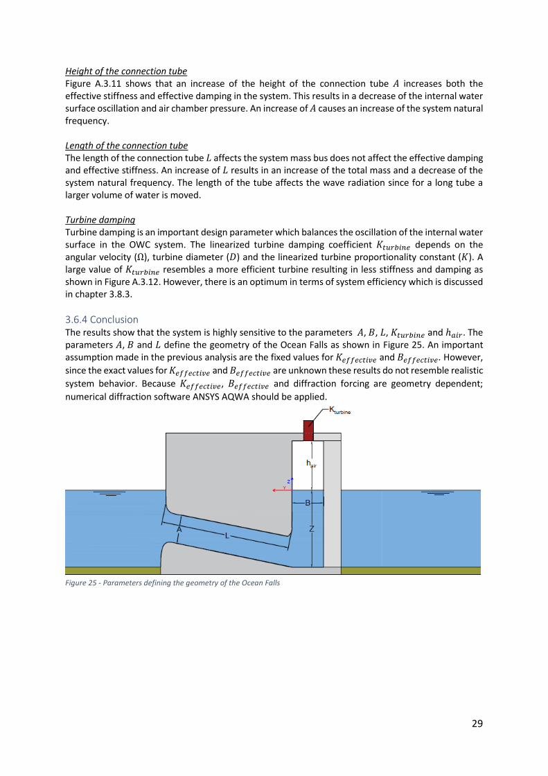
29

Height of the connection tube Figure A.3.11 shows that an increase of the height of the connection tube 𝐴 increases both the effective stiffness and effective damping in the system. This results in a decrease of the internal water surface oscillation and air chamber pressure. An increase of 𝐴 causes an increase of the system natural frequency. Length of the connection tube The length of the connection tube 𝐿 affects the system mass bus does not affect the effective damping and effective stiffness. An increase of 𝐿 results in an increase of the total mass and a decrease of the system natural frequency. The length of the tube affects the wave radiation since for a long tube a larger volume of water is moved. Turbine damping Turbine damping is an important design parameter which balances the oscillation of the internal water surface in the OWC system. The linearized turbine damping coefficient 𝐾𝑡𝑢𝑟𝑏𝑖𝑛𝑒 depends on the angular velocity (Ω), turbine diameter (𝐷) and the linearized turbine proportionality constant (𝐾). A large value of 𝐾𝑡𝑢𝑟𝑏𝑖𝑛𝑒 resembles a more efficient turbine resulting in less stiffness and damping as shown in Figure A.3.12. However, there is an optimum in terms of system efficiency which is discussed in chapter 3.8.3.

3.6.4 Conclusion The results show that the system is highly sensitive to the parameters 𝐴, 𝐵, 𝐿, 𝐾𝑡𝑢𝑟𝑏𝑖𝑛𝑒 and ℎ𝑎𝑖𝑟. The parameters 𝐴, 𝐵 and 𝐿 define the geometry of the Ocean Falls as shown in Figure 25. An important assumption made in the previous analysis are the fixed values for 𝐾𝑒𝑓𝑓𝑒𝑐𝑡𝑖𝑣𝑒 and 𝐵𝑒𝑓𝑓𝑒𝑐𝑡𝑖𝑣𝑒. However,

since the exact values for 𝐾𝑒𝑓𝑓𝑒𝑐𝑡𝑖𝑣𝑒 and 𝐵𝑒𝑓𝑓𝑒𝑐𝑡𝑖𝑣𝑒 are unknown these results do not resemble realistic

system behavior. Because 𝐾𝑒𝑓𝑓𝑒𝑐𝑡𝑖𝑣𝑒, 𝐵𝑒𝑓𝑓𝑒𝑐𝑡𝑖𝑣𝑒 and diffraction forcing are geometry dependent;

numerical diffraction software ANSYS AQWA should be applied.

Figure 25 - Parameters defining the geometry of the Ocean Falls

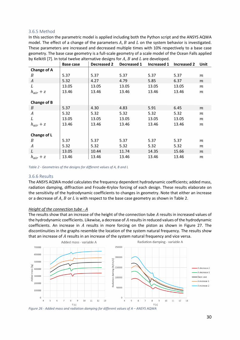
30

3.6.5 Method In this section the parametric model is applied including both the Python script and the ANSYS AQWA model. The effect of a change of the parameters 𝐴, 𝐵 and 𝐿 on the system behavior is investigated. These parameters are increased and decreased multiple times with 10% respectively to a base case geometry. The base case geometry is a full-scale geometry of a scale model of the Ocean Falls applied by Kelkitli [7]. In total twelve alternative designs for 𝐴, 𝐵 and 𝐿 are developed.

Base case Decreased 2 Decreased 1 Increased 1 Increased 2 Unit

Change of A 𝐵 5.37 5.37 5.37 5.37 5.37 𝑚 𝐴 5.32 4.27 4.79 5.85 6.37 𝑚 𝐿 13.05 13.05 13.05 13.05 13.05 𝑚 ℎ𝑎𝑖𝑟 + 𝑧 13.46 13.46 13.46 13.46 13.46 𝑚 Change of B 𝐵 5.37 4.30 4.83 5.91 6.45 𝑚 𝐴 5.32 5.32 5.32 5.32 5.32 𝑚 𝐿 13.05 13.05 13.05 13.05 13.05 𝑚 ℎ𝑎𝑖𝑟 + 𝑧 13.46 13.46 13.46 13.46 13.46 𝑚 Change of L 𝐵 5.37 5.37 5.37 5.37 5.37 𝑚 𝐴 5.32 5.32 5.32 5.32 5.32 𝑚 𝐿 13.05 10.44 11.74 14.35 15.66 𝑚 ℎ𝑎𝑖𝑟 + 𝑧 13.46 13.46 13.46 13.46 13.46 𝑚

Table 2 - Geometries of the designs for different values of A, B and L

3.6.6 Results The ANSYS AQWA model calculates the frequency dependent hydrodynamic coefficients; added mass, radiation damping, diffraction and Froude-Krylov forcing of each design. These results elaborate on the sensitivity of the hydrodynamic coefficients to changes in geometry. Note that either an increase or a decrease of 𝐴, 𝐵 or 𝐿 is with respect to the base case geometry as shown in Table 2. Height of the connection tube - A The results show that an increase of the height of the connection tube 𝐴 results in increased values of the hydrodynamic coefficients. Likewise, a decrease of 𝐴 results in reduced values of the hydrodynamic coefficients. An increase in 𝐴 results in more forcing on the piston as shown in Figure 27. The discontinuities in the graphs resemble the location of the system natural frequency. The results show that an increase of 𝐴 results in an increase of the system natural frequency and vice versa.

Figure 26 - Added mass and radiation damping for different values of A – ANSYS AQWA

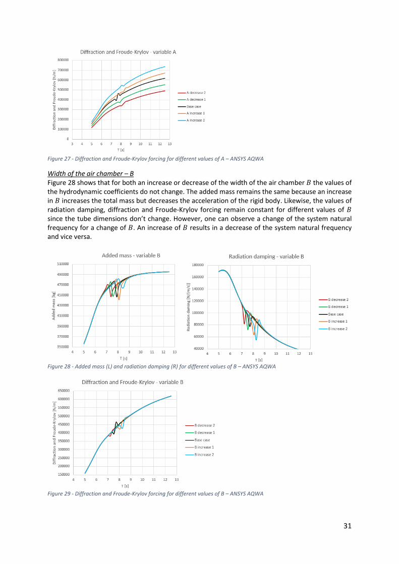
31

Figure 27 - Diffraction and Froude-Krylov forcing for different values of A – ANSYS AQWA

Width of the air chamber – B Figure 28 shows that for both an increase or decrease of the width of the air chamber 𝐵 the values of the hydrodynamic coefficients do not change. The added mass remains the same because an increase in 𝐵 increases the total mass but decreases the acceleration of the rigid body. Likewise, the values of radiation damping, diffraction and Froude-Krylov forcing remain constant for different values of 𝐵 since the tube dimensions don’t change. However, one can observe a change of the system natural frequency for a change of 𝐵. An increase of 𝐵 results in a decrease of the system natural frequency and vice versa.

Figure 28 - Added mass (L) and radiation damping (R) for different values of B – ANSYS AQWA

Figure 29 - Diffraction and Froude-Krylov forcing for different values of B – ANSYS AQWA

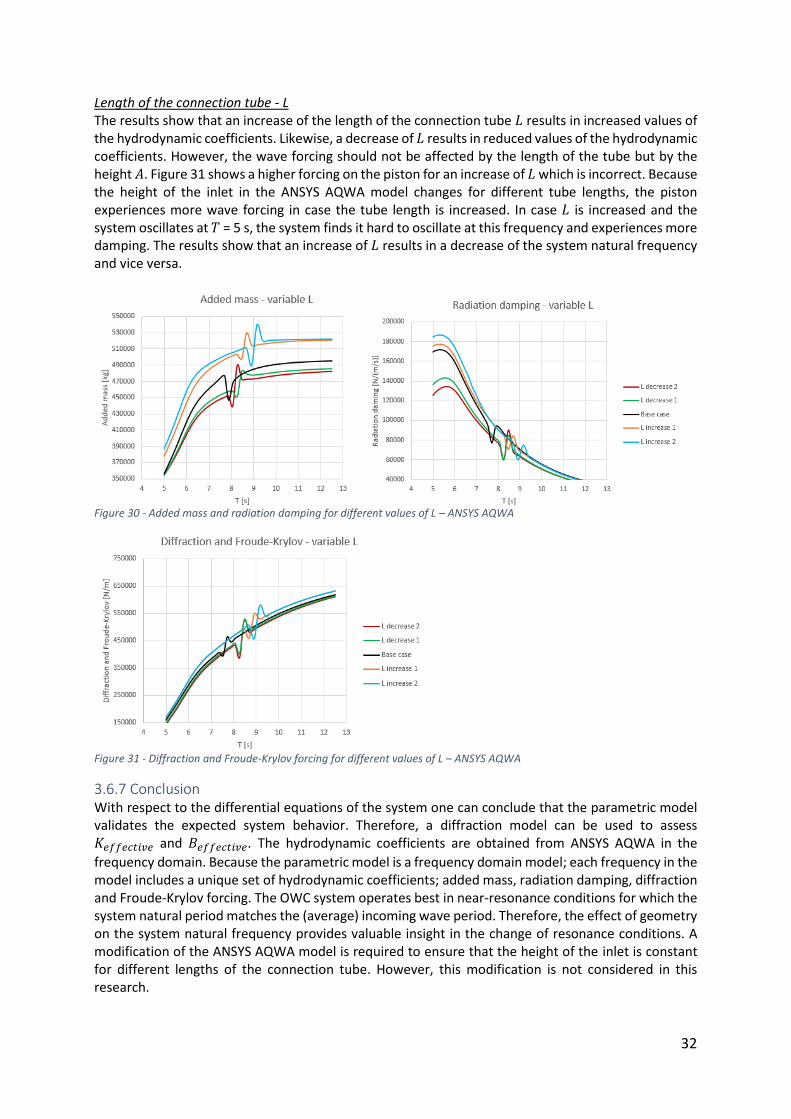
32

Length of the connection tube - L The results show that an increase of the length of the connection tube 𝐿 results in increased values of the hydrodynamic coefficients. Likewise, a decrease of 𝐿 results in reduced values of the hydrodynamic coefficients. However, the wave forcing should not be affected by the length of the tube but by the height 𝐴. Figure 31 shows a higher forcing on the piston for an increase of 𝐿 which is incorrect. Because the height of the inlet in the ANSYS AQWA model changes for different tube lengths, the piston experiences more wave forcing in case the tube length is increased. In case 𝐿 is increased and the system oscillates at 𝑇 = 5 s, the system finds it hard to oscillate at this frequency and experiences more damping. The results show that an increase of 𝐿 results in a decrease of the system natural frequency and vice versa.

Figure 30 - Added mass and radiation damping for different values of L – ANSYS AQWA

Figure 31 - Diffraction and Froude-Krylov forcing for different values of L – ANSYS AQWA

3.6.7 Conclusion With respect to the differential equations of the system one can conclude that the parametric model validates the expected system behavior. Therefore, a diffraction model can be used to assess 𝐾𝑒𝑓𝑓𝑒𝑐𝑡𝑖𝑣𝑒 and 𝐵𝑒𝑓𝑓𝑒𝑐𝑡𝑖𝑣𝑒. The hydrodynamic coefficients are obtained from ANSYS AQWA in the

frequency domain. Because the parametric model is a frequency domain model; each frequency in the model includes a unique set of hydrodynamic coefficients; added mass, radiation damping, diffraction and Froude-Krylov forcing. The OWC system operates best in near-resonance conditions for which the system natural period matches the (average) incoming wave period. Therefore, the effect of geometry on the system natural frequency provides valuable insight in the change of resonance conditions. A modification of the ANSYS AQWA model is required to ensure that the height of the inlet is constant for different lengths of the connection tube. However, this modification is not considered in this research.

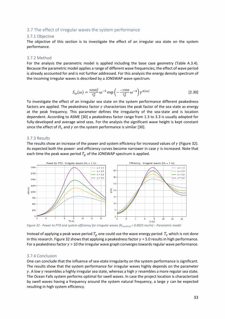
33

3.7 The effect of irregular waves the system performance

3.7.1 Objective The objective of this section is to investigate the effect of an irregular sea state on the system performance.

3.7.2 Method For the analysis the parametric model is applied including the base case geometry (Table A.3.4). Because the parametric model applies a range of different wave frequencies; the effect of wave period is already accounted for and is not further addressed. For this analysis the energy density spectrum of the incoming irregular waves is described by a JONSWAP wave spectrum.

To investigate the effect of an irregular sea state on the system performance different peakedness factors are applied. The peakedness factor 𝛾 characterizes the peak factor of the sea state as energy at the peak frequency. This parameter defines the irregularity of the sea-state and is location dependent. According to ASME [30] a peakedness factor range from 1.3 to 3.3 is usually adopted for fully-developed and average wind seas. For the analysis the significant wave height is kept constant since the effect of 𝐻𝑠 and 𝛾 on the system performance is similar [30].

3.7.3 Results The results show an increase of the power and system efficiency for increased values of 𝛾 (Figure 32). As expected both the power- and efficiency curves become narrower in case 𝛾 is increased. Note that each time the peak wave period 𝑇𝑝 of the JONSWAP spectrum is applied.

Figure 32 - Power to PTO and system efficiency for irregular waves (𝐾𝑡𝑢𝑟𝑏𝑖𝑛𝑒= 0.0025 ms/m) – Parametric model

Instead of applying a peak wave period 𝑇𝑝 one could use the wave energy period 𝑇𝑒 which is not done

in this research. Figure 32 shows that applying a peakedness factor 𝛾 = 5.0 results in high performance. For a peakedness factor 𝛾 > 10 the irregular wave graph converges towards regular wave performance.

3.7.4 Conclusion One can conclude that the influence of sea-state irregularity on the system performance is significant. The results show that the system performance for irregular waves highly depends on the parameter 𝛾. A low 𝛾 resembles a highly irregular sea state, whereas a high 𝛾 resembles a more regular sea state. The Ocean Falls system performs optimal for swell waves. In case the project location is characterized by swell waves having a frequency around the system natural frequency, a large 𝛾 can be expected resulting in high system efficiency.

𝑆ω(𝜔) =320𝐻𝑠

2

𝑇𝑝4 ω−5 exp (−

−1950

𝑇𝑝4 𝜔−4) 𝛾𝛼(𝜔) [2.30]

[2.2]

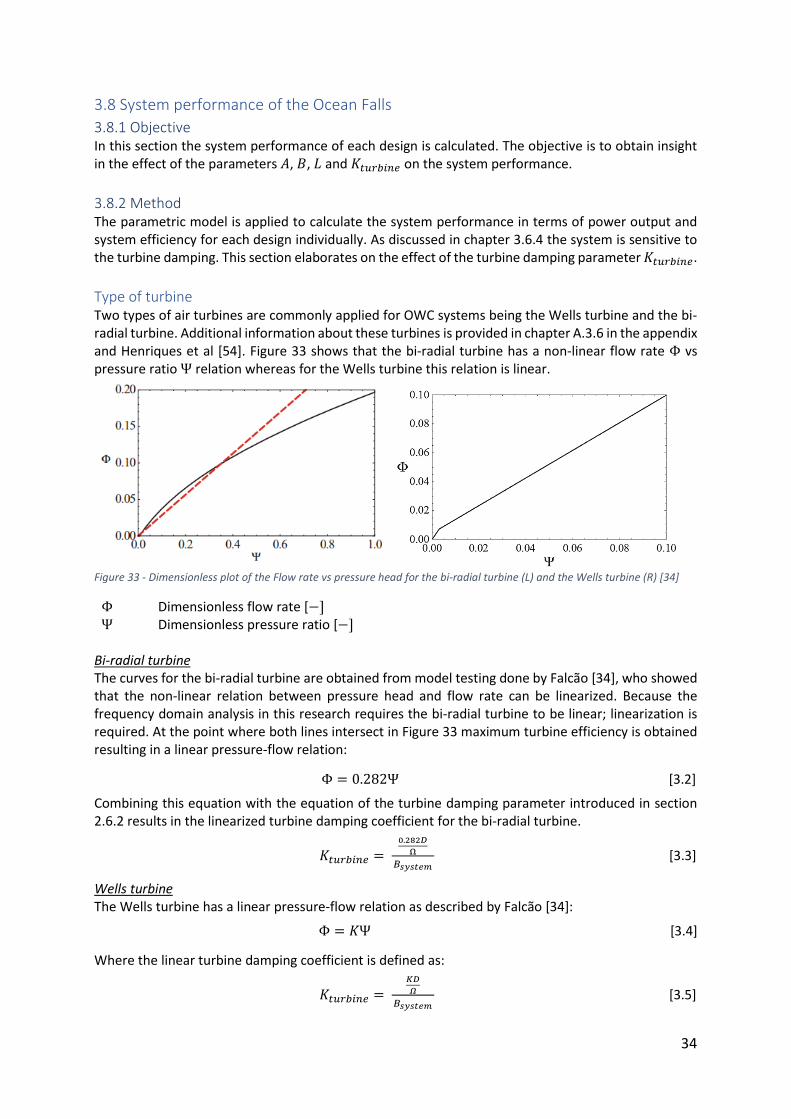
34

Φ = 0.282Ψ [3.2]

[2.2]

Φ = 𝐾Ψ [3.4]

[2.2]

3.8 System performance of the Ocean Falls

3.8.1 Objective In this section the system performance of each design is calculated. The objective is to obtain insight in the effect of the parameters 𝐴, 𝐵, 𝐿 and 𝐾𝑡𝑢𝑟𝑏𝑖𝑛𝑒 on the system performance.

3.8.2 Method The parametric model is applied to calculate the system performance in terms of power output and system efficiency for each design individually. As discussed in chapter 3.6.4 the system is sensitive to the turbine damping. This section elaborates on the effect of the turbine damping parameter 𝐾𝑡𝑢𝑟𝑏𝑖𝑛𝑒.

Type of turbine Two types of air turbines are commonly applied for OWC systems being the Wells turbine and the bi-radial turbine. Additional information about these turbines is provided in chapter A.3.6 in the appendix and Henriques et al [54]. Figure 33 shows that the bi-radial turbine has a non-linear flow rate Φ vs pressure ratio Ψ relation whereas for the Wells turbine this relation is linear.

Figure 33 - Dimensionless plot of the Flow rate vs pressure head for the bi-radial turbine (L) and the Wells turbine (R) [34]

Φ Dimensionless flow rate [−] Ψ Dimensionless pressure ratio [−]

Bi-radial turbine The curves for the bi-radial turbine are obtained from model testing done by Falcao [34], who showed that the non-linear relation between pressure head and flow rate can be linearized. Because the frequency domain analysis in this research requires the bi-radial turbine to be linear; linearization is required. At the point where both lines intersect in Figure 33 maximum turbine efficiency is obtained resulting in a linear pressure-flow relation: Combining this equation with the equation of the turbine damping parameter introduced in section 2.6.2 results in the linearized turbine damping coefficient for the bi-radial turbine.

Wells turbine The Wells turbine has a linear pressure-flow relation as described by Falcao [34]: Where the linear turbine damping coefficient is defined as:

𝐾𝑡𝑢𝑟𝑏𝑖𝑛𝑒 = 0.282𝐷

Ω

𝐵𝑠𝑦𝑠𝑡𝑒𝑚 [3.3]

[2.2]

𝐾𝑡𝑢𝑟𝑏𝑖𝑛𝑒 =

𝐾𝐷

𝛺

𝐵𝑠𝑦𝑠𝑡𝑒𝑚 [3.5]

[2.2]

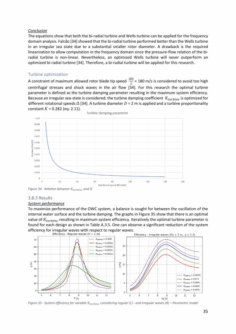
35

Conclusion The equations show that both the bi-radial turbine and Wells turbine can be applied for the frequency domain analysis. Falcao [34] showed that the bi-radial turbine performed better than the Wells turbine in an irregular sea state due to a substantial smaller rotor diameter. A drawback is the required linearization to allow computation in the frequency domain since the pressure-flow relation of the bi-radial turbine is non-linear. Nevertheless, an optimized Wells turbine will never outperform an optimized bi-radial turbine [34]. Therefore, a bi-radial turbine will be applied for this research.

Turbine optimization

A constraint of maximum allowed rotor blade tip speed ΩD

2 = 180 m/s is considered to avoid too high

centrifugal stresses and shock waves in the air flow [34]. For this research the optimal turbine parameter is defined as the turbine damping parameter resulting in the maximum system efficiency. Because an irregular sea-state is considered; the turbine damping coefficient 𝐾𝑡𝑢𝑟𝑏𝑖𝑛𝑒 is optimized for different rotational speeds Ω [34]. A turbine diameter 𝐷 = 2 m is applied and a turbine proportionality constant 𝐾 = 0.282 (eq. 2.11).

Figure 34 - Relation between 𝐾𝑡𝑢𝑟𝑏𝑖𝑛𝑒 and 𝛺

3.8.3 Results System performance To maximize performance of the OWC system, a balance is sought for between the oscillation of the internal water surface and the turbine damping. The graphs in Figure 35 show that there is an optimal value of 𝐾𝑡𝑢𝑟𝑏𝑖𝑛𝑒 resulting in maximum system efficiency. Iteratively the optimal turbine parameter is found for each design as shown in Table A.3.5. One can observe a significant reduction of the system efficiency for irregular waves with respect to regular waves.

Figure 35 - System efficiency for variable 𝐾𝑡𝑢𝑟𝑏𝑖𝑛𝑒 considering regular (L) - and irregular waves (R) – Parametric model

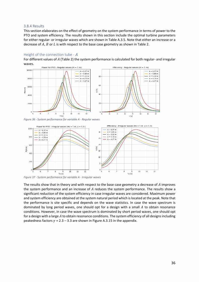
36

3.8.4 Results This section elaborates on the effect of geometry on the system performance in terms of power to the PTO and system efficiency. The results shown in this section include the optimal turbine parameters for either regular- or irregular waves which are shown in Table A.3.5. Note that either an increase or a decrease of 𝐴, 𝐵 or 𝐿 is with respect to the base case geometry as shown in Table 2.

Height of the connection tube - 𝐴 For different values of 𝐴 (Table 2) the system performance is calculated for both regular- and irregular waves.

Figure 36 - System performance for variable A - Regular waves

Figure 37 - System performance for variable A - Irregular waves

The results show that in theory and with respect to the base case geometry a decrease of 𝐴 improves the system performance and an increase of 𝐴 reduces the system performance. The results show a significant reduction of the system efficiency in case irregular waves are considered. Maximum power and system efficiency are obtained at the system natural period which is located at the peak. Note that the performance is site specific and depends on the wave statistics. In case the wave spectrum is dominated by long period waves, one should opt for a design with a small 𝐴 to obtain resonance conditions. However, in case the wave spectrum is dominated by short period waves, one should opt for a design with a large 𝐴 to obtain resonance conditions. The system efficiency of all designs including peakedness factors 𝛾 = 2.3 – 3.3 are shown in Figure A.3.15 in the appendix.

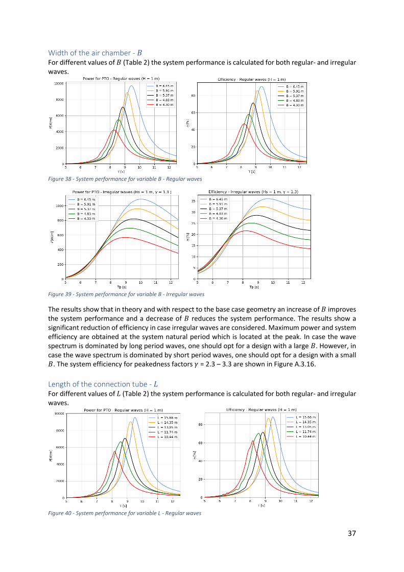
37

Width of the air chamber - 𝐵 For different values of 𝐵 (Table 2) the system performance is calculated for both regular- and irregular waves.

Figure 38 - System performance for variable B - Regular waves

Figure 39 - System performance for variable B - Irregular waves

The results show that in theory and with respect to the base case geometry an increase of 𝐵 improves the system performance and a decrease of 𝐵 reduces the system performance. The results show a significant reduction of efficiency in case irregular waves are considered. Maximum power and system efficiency are obtained at the system natural period which is located at the peak. In case the wave spectrum is dominated by long period waves, one should opt for a design with a large 𝐵. However, in case the wave spectrum is dominated by short period waves, one should opt for a design with a small 𝐵. The system efficiency for peakedness factors 𝛾 = 2.3 – 3.3 are shown in Figure A.3.16.

Length of the connection tube - 𝐿 For different values of 𝐿 (Table 2) the system performance is calculated for both regular- and irregular waves.

Figure 40 - System performance for variable L - Regular waves

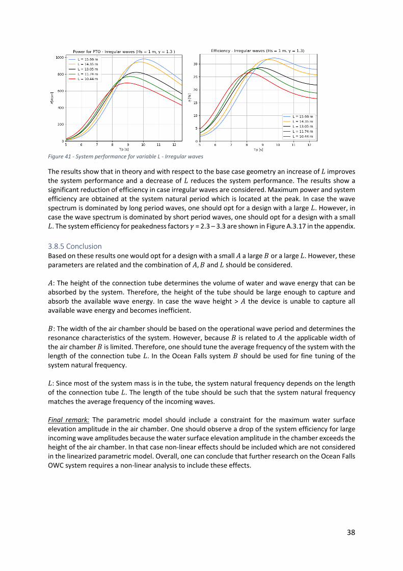
38

Figure 41 - System performance for variable L - Irregular waves

The results show that in theory and with respect to the base case geometry an increase of 𝐿 improves the system performance and a decrease of 𝐿 reduces the system performance. The results show a significant reduction of efficiency in case irregular waves are considered. Maximum power and system efficiency are obtained at the system natural period which is located at the peak. In case the wave spectrum is dominated by long period waves, one should opt for a design with a large 𝐿. However, in case the wave spectrum is dominated by short period waves, one should opt for a design with a small 𝐿. The system efficiency for peakedness factors 𝛾 = 2.3 – 3.3 are shown in Figure A.3.17 in the appendix.

3.8.5 Conclusion Based on these results one would opt for a design with a small 𝐴 a large 𝐵 or a large 𝐿. However, these parameters are related and the combination of 𝐴, 𝐵 and 𝐿 should be considered. 𝐴: The height of the connection tube determines the volume of water and wave energy that can be absorbed by the system. Therefore, the height of the tube should be large enough to capture and absorb the available wave energy. In case the wave height > 𝐴 the device is unable to capture all available wave energy and becomes inefficient. 𝐵: The width of the air chamber should be based on the operational wave period and determines the resonance characteristics of the system. However, because 𝐵 is related to 𝐴 the applicable width of the air chamber 𝐵 is limited. Therefore, one should tune the average frequency of the system with the length of the connection tube 𝐿. In the Ocean Falls system 𝐵 should be used for fine tuning of the system natural frequency. 𝐿: Since most of the system mass is in the tube, the system natural frequency depends on the length of the connection tube 𝐿. The length of the tube should be such that the system natural frequency matches the average frequency of the incoming waves. Final remark: The parametric model should include a constraint for the maximum water surface elevation amplitude in the air chamber. One should observe a drop of the system efficiency for large incoming wave amplitudes because the water surface elevation amplitude in the chamber exceeds the height of the air chamber. In that case non-linear effects should be included which are not considered in the linearized parametric model. Overall, one can conclude that further research on the Ocean Falls OWC system requires a non-linear analysis to include these effects.

39

3.9 CFD model

3.9.1 Objective For this research a 2D Computational Fluid Dynamics model (CFD) of the Ocean Falls is set up. The objective is to obtain insight in the system behavior and the influence of non-linear hydrodynamic effects. With respect to the parametric model the CFD model has several advantages:

- Allows for large wave- and body motions and can deal with resonating water surfaces - Able to deal with complexities in geometry e.g. curves and sharp edges - Able to describe a non-linear pressure flow relation - Allows the use of a multiphase model which separates water and air - Includes the effect of viscous friction, turbulence, vortex shedding and dissipation of energy

from other non-linear phenomena. The CFD model is applied to assess the validity of the linearized parametric model, understand the differences and identify model limitations. Several research questions are defined:

I. Is the capacity of the current design sufficient to accommodate the total volume of water? II. Does the CFD model with or without air chamber pressure validate the results obtained from

the parametric model? III. Does the outlet modelled in CFD resemble the correct turbine damping coefficient 𝐾𝑡𝑢𝑟𝑏𝑖𝑛𝑒? IV. What is the advantage of the Ocean Falls OWC system with respect to conventional OWC

systems? V. What is the effect of marine growth on the system response?

VI. What is the effect of variable and constant air density on the system response?

3.9.2 Method Appendix chapter A.3.7 elaborates on how the CFD model is made, applied settings, boundary conditions, type of forcing and calculation procedures. A wave tank length of 3 times the maximum wave length is applied to minimize the effect of wave reflection. However, since the wave boundary is reflective, wave reflection will occur. A wave reflection analysis is done to obtain insight in the effect of wave reflection. Figure A.3.20 in the appendix shows a difference in maximum internal water surface elevation amplitude of 12% which is likely due to wave reflection from the reflective wave boundary. Before the CFD model can be applied and used for comparison; the accuracy of the CFD model should be assessed. Therefore, the results obtained from model scale experiments of the Ocean Falls done by Kelkitli [7] are compared with the results obtained from the CFD model.

Experiments The internal water surface elevation amplitude �� is calculated by the CFD model and compared with the results obtained from model scale experiments. A detailed description of the experimental set-up and characteristics is provided by Kelkitli [7]. Key experiment characteristics are:

• The experiments are performed using Froude scaling with a scale factor 𝜖 = 30

• The water surface elevation is recorded at a frequency of 32 Hz

• Experiments are performed in a constant water depth of 0.5 m

• Regular waves with a wave period 𝑇 = 0.85 s - 𝑇 = 5.0 s and wavelengths 𝐿 = 1.12 s - 𝐿 = 10.9 s

• Fixed incoming wave amplitude of 0.03 m

• Distance from scale model to the wave generator of 10.47 m

• Open chamber conditions

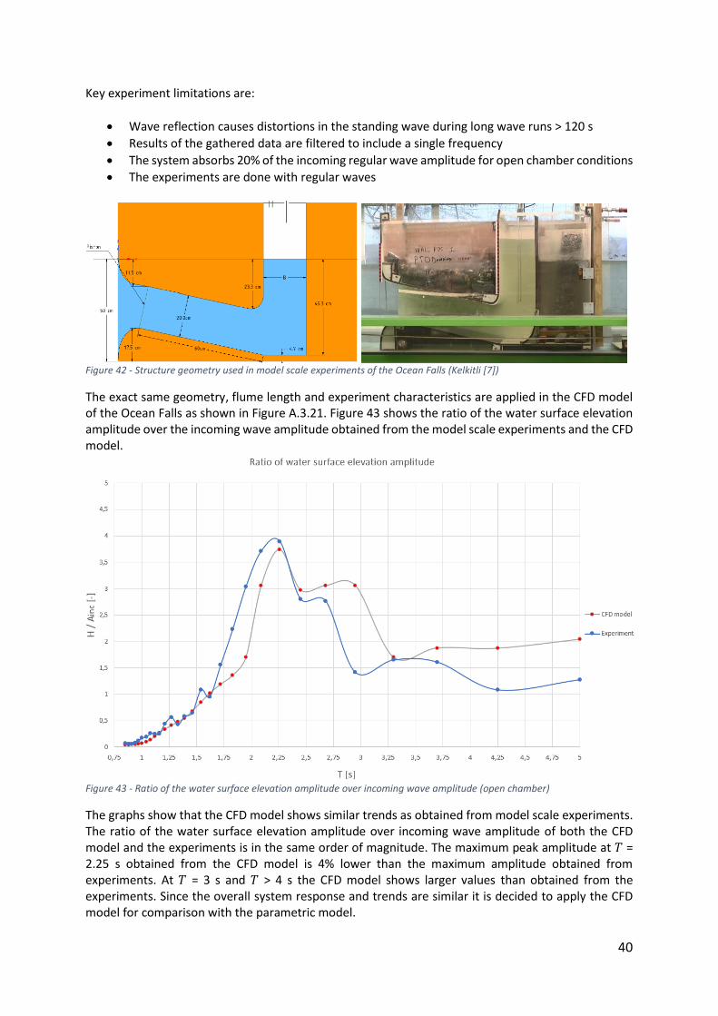
40

Key experiment limitations are:

• Wave reflection causes distortions in the standing wave during long wave runs > 120 s

• Results of the gathered data are filtered to include a single frequency

• The system absorbs 20% of the incoming regular wave amplitude for open chamber conditions

• The experiments are done with regular waves

Figure 42 - Structure geometry used in model scale experiments of the Ocean Falls (Kelkitli [7])

The exact same geometry, flume length and experiment characteristics are applied in the CFD model of the Ocean Falls as shown in Figure A.3.21. Figure 43 shows the ratio of the water surface elevation amplitude over the incoming wave amplitude obtained from the model scale experiments and the CFD model.

Figure 43 - Ratio of the water surface elevation amplitude over incoming wave amplitude (open chamber)

The graphs show that the CFD model shows similar trends as obtained from model scale experiments. The ratio of the water surface elevation amplitude over incoming wave amplitude of both the CFD model and the experiments is in the same order of magnitude. The maximum peak amplitude at 𝑇 = 2.25 s obtained from the CFD model is 4% lower than the maximum amplitude obtained from experiments. At 𝑇 = 3 s and 𝑇 > 4 s the CFD model shows larger values than obtained from the experiments. Since the overall system response and trends are similar it is decided to apply the CFD model for comparison with the parametric model.

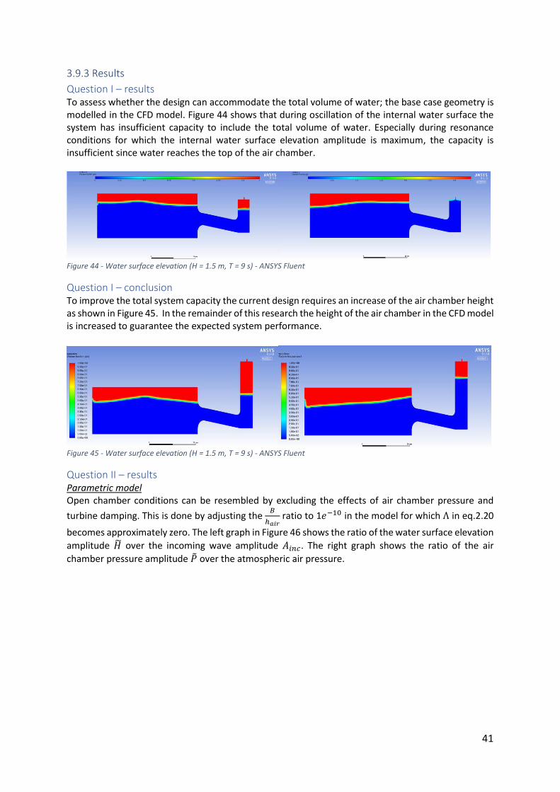
41

3.9.3 Results

Question I – results To assess whether the design can accommodate the total volume of water; the base case geometry is modelled in the CFD model. Figure 44 shows that during oscillation of the internal water surface the system has insufficient capacity to include the total volume of water. Especially during resonance conditions for which the internal water surface elevation amplitude is maximum, the capacity is insufficient since water reaches the top of the air chamber.

Figure 44 - Water surface elevation (H = 1.5 m, T = 9 s) - ANSYS Fluent

Question I – conclusion To improve the total system capacity the current design requires an increase of the air chamber height as shown in Figure 45. In the remainder of this research the height of the air chamber in the CFD model is increased to guarantee the expected system performance.

Figure 45 - Water surface elevation (H = 1.5 m, T = 9 s) - ANSYS Fluent

Question II – results Parametric model Open chamber conditions can be resembled by excluding the effects of air chamber pressure and

turbine damping. This is done by adjusting the 𝐵

ℎ𝑎𝑖𝑟 ratio to 1𝑒−10 in the model for which Λ in eq.2.20

becomes approximately zero. The left graph in Figure 46 shows the ratio of the water surface elevation

amplitude �� over the incoming wave amplitude 𝐴𝑖𝑛𝑐. The right graph shows the ratio of the air

chamber pressure amplitude �� over the atmospheric air pressure.

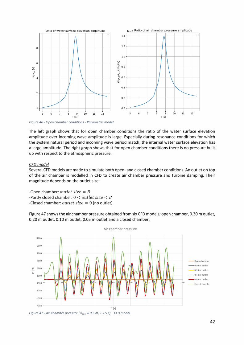
42

Figure 46 - Open chamber conditions - Parametric model

The left graph shows that for open chamber conditions the ratio of the water surface elevation amplitude over incoming wave amplitude is large. Especially during resonance conditions for which the system natural period and incoming wave period match; the internal water surface elevation has a large amplitude. The right graph shows that for open chamber conditions there is no pressure built up with respect to the atmospheric pressure. CFD model Several CFD models are made to simulate both open- and closed chamber conditions. An outlet on top of the air chamber is modelled in CFD to create air chamber pressure and turbine damping. Their magnitude depends on the outlet size: -Open chamber: 𝑜𝑢𝑡𝑙𝑒𝑡 𝑠𝑖𝑧𝑒 = 𝐵 -Partly closed chamber: 0 < 𝑜𝑢𝑡𝑙𝑒𝑡 𝑠𝑖𝑧𝑒 < 𝐵 -Closed chamber: 𝑜𝑢𝑡𝑙𝑒𝑡 𝑠𝑖𝑧𝑒 = 0 (no outlet) Figure 47 shows the air chamber pressure obtained from six CFD models; open chamber, 0.30 m outlet, 0.20 m outlet, 0.10 m outlet, 0.05 m outlet and a closed chamber.

Figure 47 - Air chamber pressure (𝐴𝑖𝑛𝑐 = 0.5 m, T = 9 s) – CFD model

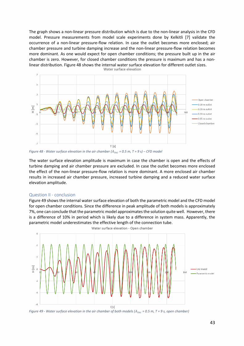
43

The graph shows a non-linear pressure distribution which is due to the non-linear analysis in the CFD model. Pressure measurements from model scale experiments done by Kelkitli [7] validate the occurrence of a non-linear pressure-flow relation. In case the outlet becomes more enclosed; air chamber pressure and turbine damping increase and the non-linear pressure-flow relation becomes more dominant. As one would expect for open chamber conditions; the pressure built up in the air chamber is zero. However, for closed chamber conditions the pressure is maximum and has a non-linear distribution. Figure 48 shows the internal water surface elevation for different outlet sizes.

Figure 48 - Water surface elevation in the air chamber (𝐴𝑖𝑛𝑐 = 0.5 m, T = 9 s) – CFD model

The water surface elevation amplitude is maximum in case the chamber is open and the effects of turbine damping and air chamber pressure are excluded. In case the outlet becomes more enclosed the effect of the non-linear pressure-flow relation is more dominant. A more enclosed air chamber results in increased air chamber pressure, increased turbine damping and a reduced water surface elevation amplitude.

Question II - conclusion Figure 49 shows the internal water surface elevation of both the parametric model and the CFD model for open chamber conditions. Since the difference in peak amplitude of both models is approximately 7%, one can conclude that the parametric model approximates the solution quite well. However, there is a difference of 10% in period which is likely due to a difference in system mass. Apparently, the parametric model underestimates the effective length of the connection tube.

Figure 49 - Water surface elevation in the air chamber of both models (𝐴𝑖𝑛𝑐 = 0.5 m, T = 9 s, open chamber)

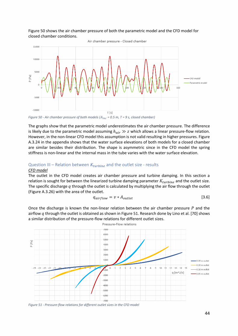
44

Figure 50 shows the air chamber pressure of both the parametric model and the CFD model for closed chamber conditions.

Figure 50 - Air chamber pressure of both models (𝐴𝑖𝑛𝑐 = 0.5 m, T = 9 s, closed chamber)

The graphs show that the parametric model underestimates the air chamber pressure. The difference is likely due to the parametric model assuming ℎ𝑎𝑖𝑟 ≫ 𝑧 which allows a linear pressure-flow relation. However, in the non-linear CFD model this assumption is not valid resulting in higher pressures. Figure A.3.24 in the appendix shows that the water surface elevations of both models for a closed chamber are similar besides their distribution. The shape is asymmetric since in the CFD model the spring stiffness is non-linear and the internal mass in the tube varies with the water surface elevation.

Question III – Relation between 𝐾𝑡𝑢𝑟𝑏𝑖𝑛𝑒 and the outlet size - results CFD model The outlet in the CFD model creates air chamber pressure and turbine damping. In this section a relation is sought for between the linearized turbine damping parameter 𝐾𝑡𝑢𝑟𝑏𝑖𝑛𝑒 and the outlet size. The specific discharge 𝑞 through the outlet is calculated by multiplying the air flow through the outlet (Figure A.3.26) with the area of the outlet.

𝑞𝑎𝑖𝑟𝑓𝑙𝑜𝑤 = 𝑣 ∗ 𝐴𝑜𝑢𝑡𝑙𝑒𝑡 [3.6]

Once the discharge is known the non-linear relation between the air chamber pressure 𝑃 and the airflow 𝑞 through the outlet is obtained as shown in Figure 51. Research done by Lino et al. [70] shows a similar distribution of the pressure-flow relations for different outlet sizes.

Figure 51 - Pressure-flow relations for different outlet sizes in the CFD model

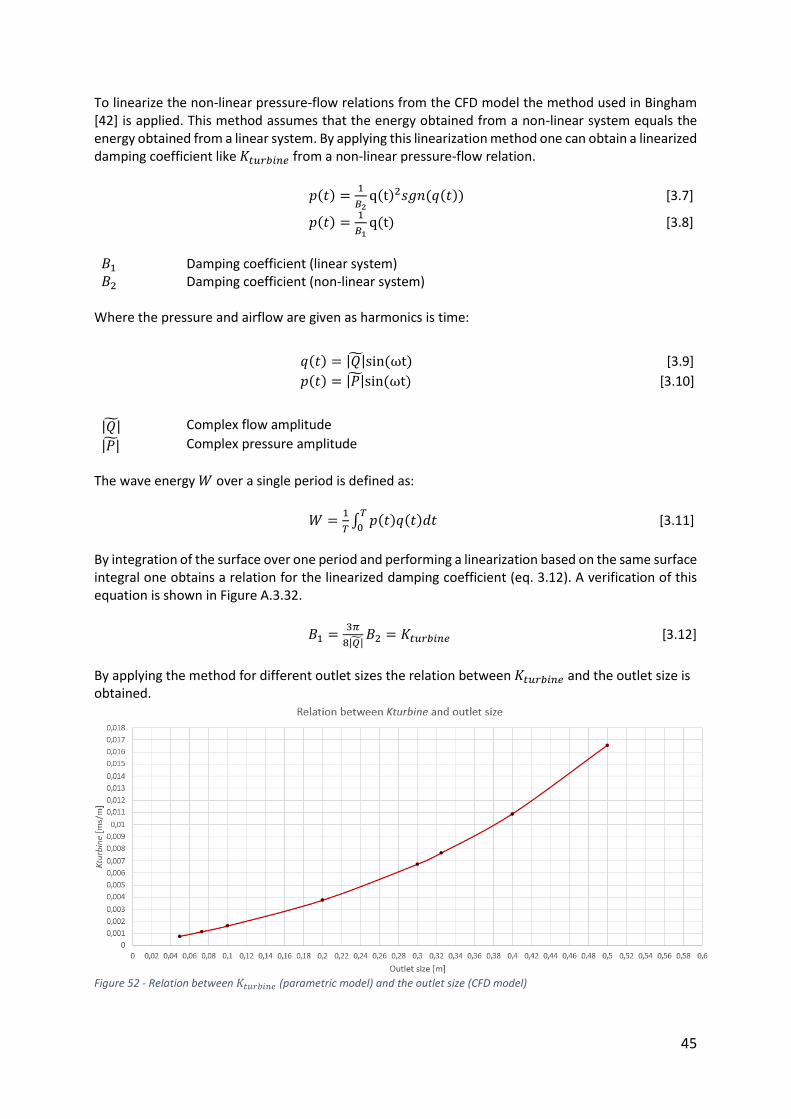
45

To linearize the non-linear pressure-flow relations from the CFD model the method used in Bingham [42] is applied. This method assumes that the energy obtained from a non-linear system equals the energy obtained from a linear system. By applying this linearization method one can obtain a linearized damping coefficient like 𝐾𝑡𝑢𝑟𝑏𝑖𝑛𝑒 from a non-linear pressure-flow relation.

𝑝(𝑡) =1

𝐵2q(t)2𝑠𝑔𝑛(𝑞(𝑡)) [3.7]

𝑝(𝑡) =1

𝐵1q(t) [3.8]

𝐵1 Damping coefficient (linear system) 𝐵2 Damping coefficient (non-linear system)

Where the pressure and airflow are given as harmonics is time:

|𝑄| Complex flow amplitude

|𝑃| Complex pressure amplitude

The wave energy 𝑊 over a single period is defined as:

𝑊 =1

𝑇∫ 𝑝(𝑡)𝑞(𝑡)𝑑𝑡

𝑇

0 [3.11]

By integration of the surface over one period and performing a linearization based on the same surface integral one obtains a relation for the linearized damping coefficient (eq. 3.12). A verification of this equation is shown in Figure A.3.32.

𝐵1 =3𝜋

8|𝑄|𝐵2 = 𝐾𝑡𝑢𝑟𝑏𝑖𝑛𝑒 [3.12]

By applying the method for different outlet sizes the relation between 𝐾𝑡𝑢𝑟𝑏𝑖𝑛𝑒 and the outlet size is obtained.

Figure 52 - Relation between 𝐾𝑡𝑢𝑟𝑏𝑖𝑛𝑒 (parametric model) and the outlet size (CFD model)

𝑞(𝑡) = |𝑄|sin (ωt) [3.9]

𝑝(𝑡) = |𝑃|sin (ωt) [3.10]

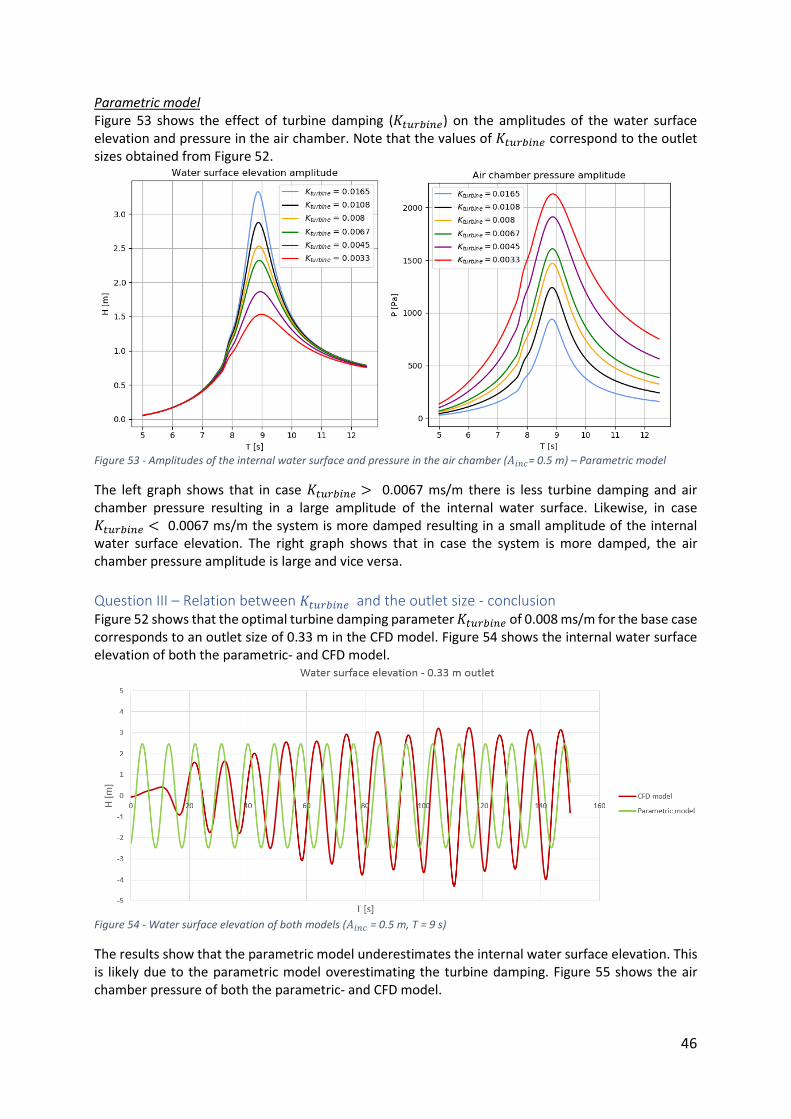
46

Parametric model Figure 53 shows the effect of turbine damping (𝐾𝑡𝑢𝑟𝑏𝑖𝑛𝑒) on the amplitudes of the water surface elevation and pressure in the air chamber. Note that the values of 𝐾𝑡𝑢𝑟𝑏𝑖𝑛𝑒 correspond to the outlet sizes obtained from Figure 52.

Figure 53 - Amplitudes of the internal water surface and pressure in the air chamber (𝐴𝑖𝑛𝑐= 0.5 m) – Parametric model

The left graph shows that in case 𝐾𝑡𝑢𝑟𝑏𝑖𝑛𝑒 > 0.0067 ms/m there is less turbine damping and air chamber pressure resulting in a large amplitude of the internal water surface. Likewise, in case 𝐾𝑡𝑢𝑟𝑏𝑖𝑛𝑒 < 0.0067 ms/m the system is more damped resulting in a small amplitude of the internal water surface elevation. The right graph shows that in case the system is more damped, the air chamber pressure amplitude is large and vice versa.

Question III – Relation between 𝐾𝑡𝑢𝑟𝑏𝑖𝑛𝑒 and the outlet size - conclusion Figure 52 shows that the optimal turbine damping parameter 𝐾𝑡𝑢𝑟𝑏𝑖𝑛𝑒 of 0.008 ms/m for the base case corresponds to an outlet size of 0.33 m in the CFD model. Figure 54 shows the internal water surface elevation of both the parametric- and CFD model.

Figure 54 - Water surface elevation of both models (𝐴𝑖𝑛𝑐 = 0.5 m, T = 9 s)

The results show that the parametric model underestimates the internal water surface elevation. This is likely due to the parametric model overestimating the turbine damping. Figure 55 shows the air chamber pressure of both the parametric- and CFD model.

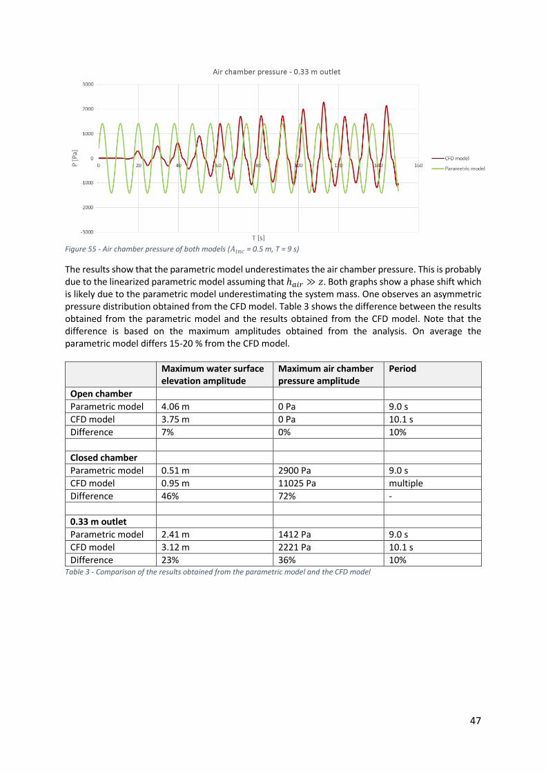
47

Figure 55 - Air chamber pressure of both models (𝐴𝑖𝑛𝑐 = 0.5 m, T = 9 s)

The results show that the parametric model underestimates the air chamber pressure. This is probably due to the linearized parametric model assuming that ℎ𝑎𝑖𝑟 ≫ 𝑧. Both graphs show a phase shift which is likely due to the parametric model underestimating the system mass. One observes an asymmetric pressure distribution obtained from the CFD model. Table 3 shows the difference between the results obtained from the parametric model and the results obtained from the CFD model. Note that the difference is based on the maximum amplitudes obtained from the analysis. On average the parametric model differs 15-20 % from the CFD model.

Maximum water surface elevation amplitude

Maximum air chamber pressure amplitude

Period

Open chamber

Parametric model 4.06 m 0 Pa 9.0 s

CFD model 3.75 m 0 Pa 10.1 s

Difference 7% 0% 10%

Closed chamber

Parametric model 0.51 m 2900 Pa 9.0 s

CFD model 0.95 m 11025 Pa multiple

Difference 46% 72% -

0.33 m outlet

Parametric model 2.41 m 1412 Pa 9.0 s

CFD model 3.12 m 2221 Pa 10.1 s

Difference 23% 36% 10% Table 3 - Comparison of the results obtained from the parametric model and the CFD model

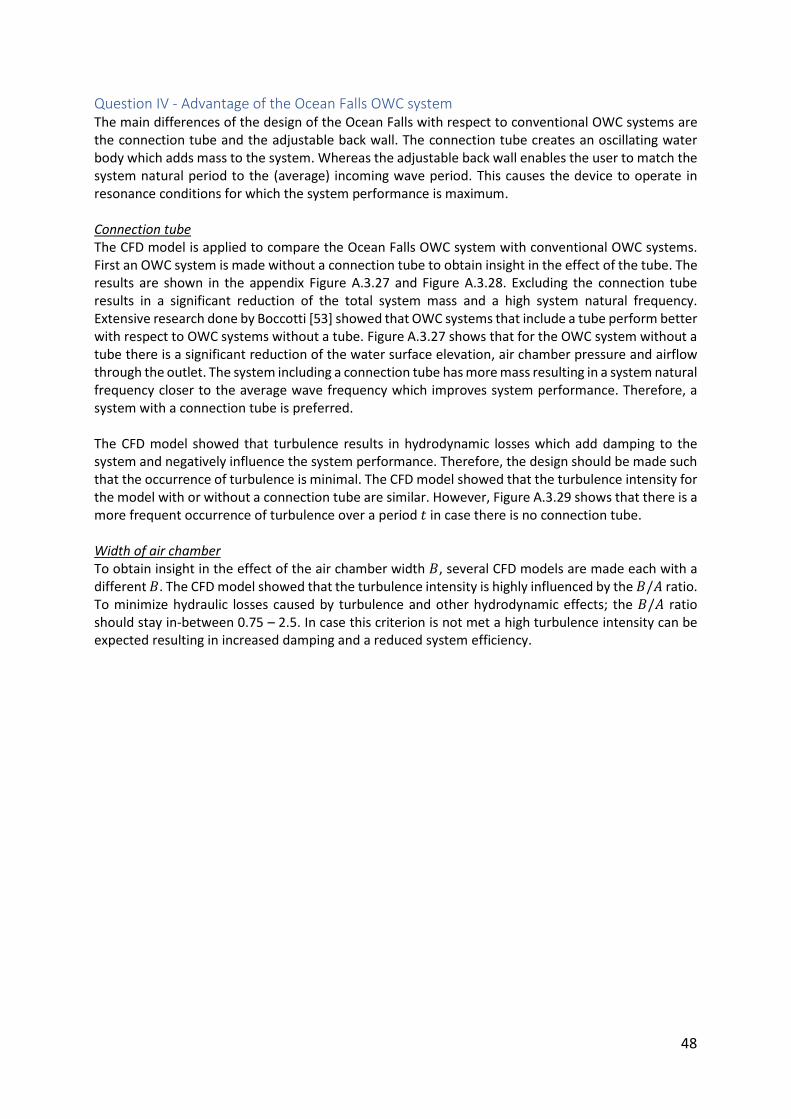
48

Question IV - Advantage of the Ocean Falls OWC system The main differences of the design of the Ocean Falls with respect to conventional OWC systems are the connection tube and the adjustable back wall. The connection tube creates an oscillating water body which adds mass to the system. Whereas the adjustable back wall enables the user to match the system natural period to the (average) incoming wave period. This causes the device to operate in resonance conditions for which the system performance is maximum. Connection tube The CFD model is applied to compare the Ocean Falls OWC system with conventional OWC systems. First an OWC system is made without a connection tube to obtain insight in the effect of the tube. The results are shown in the appendix Figure A.3.27 and Figure A.3.28. Excluding the connection tube results in a significant reduction of the total system mass and a high system natural frequency. Extensive research done by Boccotti [53] showed that OWC systems that include a tube perform better with respect to OWC systems without a tube. Figure A.3.27 shows that for the OWC system without a tube there is a significant reduction of the water surface elevation, air chamber pressure and airflow through the outlet. The system including a connection tube has more mass resulting in a system natural frequency closer to the average wave frequency which improves system performance. Therefore, a system with a connection tube is preferred. The CFD model showed that turbulence results in hydrodynamic losses which add damping to the system and negatively influence the system performance. Therefore, the design should be made such that the occurrence of turbulence is minimal. The CFD model showed that the turbulence intensity for the model with or without a connection tube are similar. However, Figure A.3.29 shows that there is a more frequent occurrence of turbulence over a period 𝑡 in case there is no connection tube. Width of air chamber To obtain insight in the effect of the air chamber width 𝐵, several CFD models are made each with a different 𝐵. The CFD model showed that the turbulence intensity is highly influenced by the 𝐵/𝐴 ratio. To minimize hydraulic losses caused by turbulence and other hydrodynamic effects; the 𝐵/𝐴 ratio should stay in-between 0.75 – 2.5. In case this criterion is not met a high turbulence intensity can be expected resulting in increased damping and a reduced system efficiency.

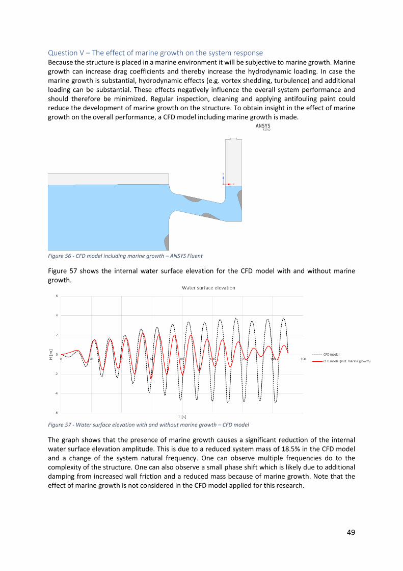
49

Question V – The effect of marine growth on the system response Because the structure is placed in a marine environment it will be subjective to marine growth. Marine growth can increase drag coefficients and thereby increase the hydrodynamic loading. In case the marine growth is substantial, hydrodynamic effects (e.g. vortex shedding, turbulence) and additional loading can be substantial. These effects negatively influence the overall system performance and should therefore be minimized. Regular inspection, cleaning and applying antifouling paint could reduce the development of marine growth on the structure. To obtain insight in the effect of marine growth on the overall performance, a CFD model including marine growth is made.

Figure 56 - CFD model including marine growth – ANSYS Fluent

Figure 57 shows the internal water surface elevation for the CFD model with and without marine growth.

Figure 57 - Water surface elevation with and without marine growth – CFD model

The graph shows that the presence of marine growth causes a significant reduction of the internal water surface elevation amplitude. This is due to a reduced system mass of 18.5% in the CFD model and a change of the system natural frequency. One can observe multiple frequencies do to the complexity of the structure. One can also observe a small phase shift which is likely due to additional damping from increased wall friction and a reduced mass because of marine growth. Note that the effect of marine growth is not considered in the CFD model applied for this research.

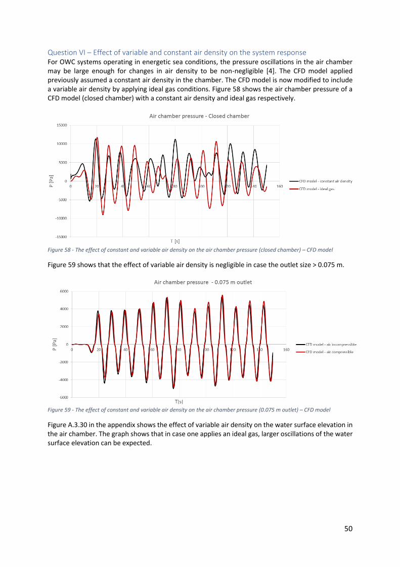
50

Question VI – Effect of variable and constant air density on the system response For OWC systems operating in energetic sea conditions, the pressure oscillations in the air chamber may be large enough for changes in air density to be non-negligible [4]. The CFD model applied previously assumed a constant air density in the chamber. The CFD model is now modified to include a variable air density by applying ideal gas conditions. Figure 58 shows the air chamber pressure of a CFD model (closed chamber) with a constant air density and ideal gas respectively.

Figure 58 - The effect of constant and variable air density on the air chamber pressure (closed chamber) – CFD model

Figure 59 shows that the effect of variable air density is negligible in case the outlet size > 0.075 m.

Figure 59 - The effect of constant and variable air density on the air chamber pressure (0.075 m outlet) – CFD model

Figure A.3.30 in the appendix shows the effect of variable air density on the water surface elevation in the air chamber. The graph shows that in case one applies an ideal gas, larger oscillations of the water surface elevation can be expected.

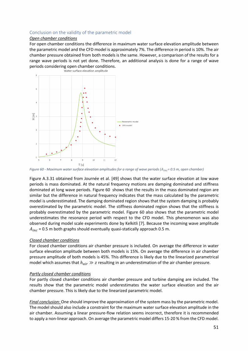
51

Conclusion on the validity of the parametric model Open chamber conditions For open chamber conditions the difference in maximum water surface elevation amplitude between the parametric model and the CFD model is approximately 7%. The difference in period is 10%. The air chamber pressure obtained from both models is the same. However, a comparison of the results for a range wave periods is not yet done. Therefore, an additional analysis is done for a range of wave periods considering open chamber conditions.

Figure 60 - Maximum water surface elevation amplitudes for a range of wave periods (𝐴𝑖𝑛𝑐= 0.5 m, open chamber)

Figure A.3.31 obtained from Journée et al. [49] shows that the water surface elevation at low wave periods is mass dominated. At the natural frequency motions are damping dominated and stiffness dominated at long wave periods. Figure 60 shows that the results in the mass dominated region are similar but the difference in natural frequency indicates that the mass calculated by the parametric model is underestimated. The damping dominated region shows that the system damping is probably overestimated by the parametric model. The stiffness dominated region shows that the stiffness is probably overestimated by the parametric model. Figure 60 also shows that the parametric model underestimates the resonance period with respect to the CFD model. This phenomenon was also observed during model scale experiments done by Kelkitli [7]. Because the incoming wave amplitude 𝐴𝑖𝑛𝑐 = 0.5 m both graphs should eventually quasi-statically approach 0.5 m. Closed chamber conditions For closed chamber conditions air chamber pressure is included. On average the difference in water surface elevation amplitude between both models is 15%. On average the difference in air chamber pressure amplitude of both models is 45%. This difference is likely due to the linearized parametrical model which assumes that ℎ𝑎𝑖𝑟 ≫ 𝑧 resulting in an underestimation of the air chamber pressure. Partly closed chamber conditions For partly closed chamber conditions air chamber pressure and turbine damping are included. The results show that the parametric model underestimates the water surface elevation and the air chamber pressure. This is likely due to the linearized parametric model. Final conclusion: One should improve the approximation of the system mass by the parametric model. The model should also include a constraint for the maximum water surface elevation amplitude in the air chamber. Assuming a linear pressure-flow relation seems incorrect, therefore it is recommended to apply a non-linear approach. On average the parametric model differs 15-20 % from the CFD model.

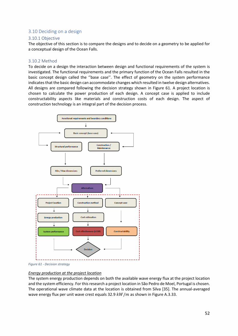
52

3.10 Deciding on a design

3.10.1 Objective The objective of this section is to compare the designs and to decide on a geometry to be applied for a conceptual design of the Ocean Falls.

3.10.2 Method To decide on a design the interaction between design and functional requirements of the system is investigated. The functional requirements and the primary function of the Ocean Falls resulted in the basic concept design called the ‘’base case’’. The effect of geometry on the system performance indicates that the basic design can accommodate changes which resulted in twelve design alternatives. All designs are compared following the decision strategy shown in Figure 61. A project location is chosen to calculate the power production of each design. A concept case is applied to include constructability aspects like materials and construction costs of each design. The aspect of construction technology is an integral part of the decision process.

Figure 61 - Decision strategy

Energy production at the project location The system energy production depends on both the available wave energy flux at the project location and the system efficiency. For this research a project location in São Pedro de Moel, Portugal is chosen. The operational wave climate data at the location is obtained from Silva [35]. The annual-averaged wave energy flux per unit wave crest equals 32.9 𝑘𝑊/𝑚 as shown in Figure A.3.33.

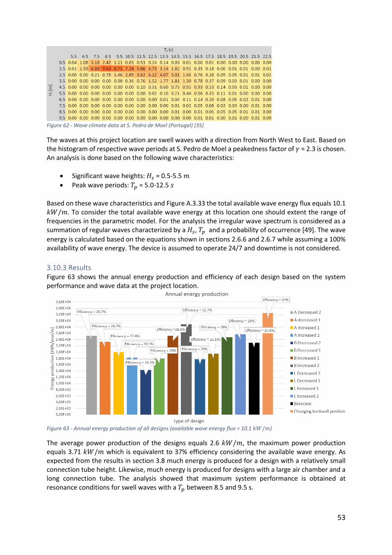
53

Figure 62 - Wave climate data at S. Pedro de Moel (Portugal) [35]

The waves at this project location are swell waves with a direction from North West to East. Based on the histogram of respective wave periods at S. Pedro de Moel a peakedness factor of 𝛾 = 2.3 is chosen. An analysis is done based on the following wave characteristics:

• Significant wave heights: 𝐻𝑠 = 0.5-5.5 𝑚

• Peak wave periods: 𝑇𝑝 = 5.0-12.5 𝑠

Based on these wave characteristics and Figure A.3.33 the total available wave energy flux equals 10.1 𝑘𝑊/𝑚. To consider the total available wave energy at this location one should extent the range of frequencies in the parametric model. For the analysis the irregular wave spectrum is considered as a summation of regular waves characterized by a 𝐻𝑠, 𝑇𝑝 and a probability of occurrence [49]. The wave

energy is calculated based on the equations shown in sections 2.6.6 and 2.6.7 while assuming a 100% availability of wave energy. The device is assumed to operate 24/7 and downtime is not considered.

3.10.3 Results Figure 63 shows the annual energy production and efficiency of each design based on the system performance and wave data at the project location.

Figure 63 - Annual energy production of all designs (available wave energy flux = 10.1 𝑘𝑊/𝑚)

The average power production of the designs equals 2.6 𝑘𝑊/𝑚, the maximum power production equals 3.71 𝑘𝑊/𝑚 which is equivalent to 37% efficiency considering the available wave energy. As expected from the results in section 3.8 much energy is produced for a design with a relatively small connection tube height. Likewise, much energy is produced for designs with a large air chamber and a long connection tube. The analysis showed that maximum system performance is obtained at resonance conditions for swell waves with a 𝑇𝑝 between 8.5 and 9.5 s.

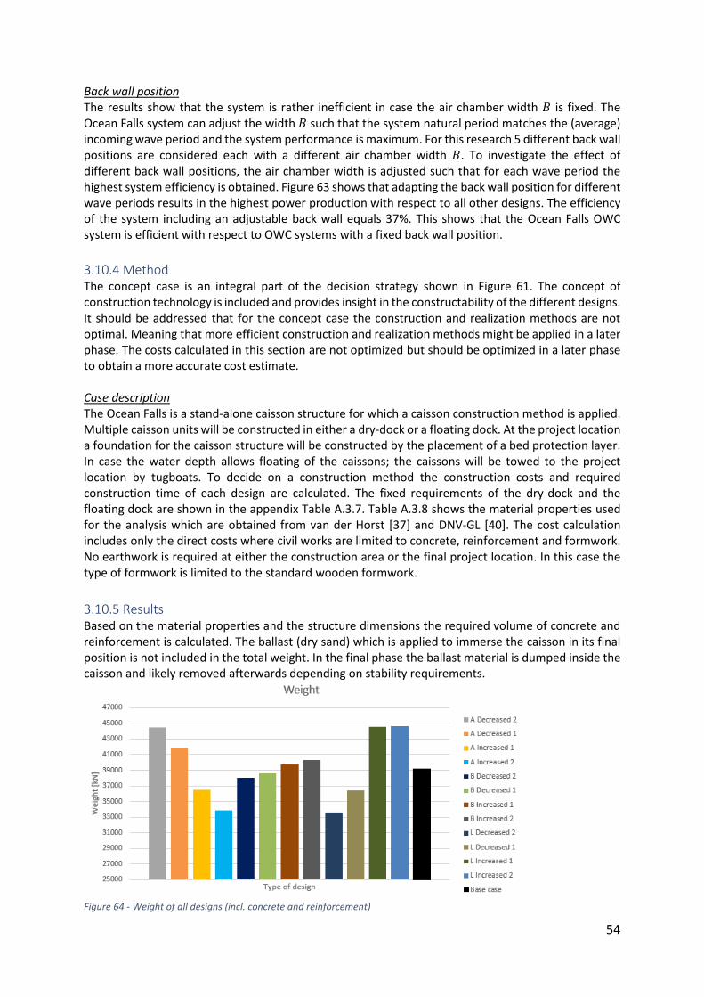
54

Back wall position The results show that the system is rather inefficient in case the air chamber width 𝐵 is fixed. The Ocean Falls system can adjust the width 𝐵 such that the system natural period matches the (average) incoming wave period and the system performance is maximum. For this research 5 different back wall positions are considered each with a different air chamber width 𝐵. To investigate the effect of different back wall positions, the air chamber width is adjusted such that for each wave period the highest system efficiency is obtained. Figure 63 shows that adapting the back wall position for different wave periods results in the highest power production with respect to all other designs. The efficiency of the system including an adjustable back wall equals 37%. This shows that the Ocean Falls OWC system is efficient with respect to OWC systems with a fixed back wall position.

3.10.4 Method The concept case is an integral part of the decision strategy shown in Figure 61. The concept of construction technology is included and provides insight in the constructability of the different designs. It should be addressed that for the concept case the construction and realization methods are not optimal. Meaning that more efficient construction and realization methods might be applied in a later phase. The costs calculated in this section are not optimized but should be optimized in a later phase to obtain a more accurate cost estimate. Case description The Ocean Falls is a stand-alone caisson structure for which a caisson construction method is applied. Multiple caisson units will be constructed in either a dry-dock or a floating dock. At the project location a foundation for the caisson structure will be constructed by the placement of a bed protection layer. In case the water depth allows floating of the caissons; the caissons will be towed to the project location by tugboats. To decide on a construction method the construction costs and required construction time of each design are calculated. The fixed requirements of the dry-dock and the floating dock are shown in the appendix Table A.3.7. Table A.3.8 shows the material properties used for the analysis which are obtained from van der Horst [37] and DNV-GL [40]. The cost calculation includes only the direct costs where civil works are limited to concrete, reinforcement and formwork. No earthwork is required at either the construction area or the final project location. In this case the type of formwork is limited to the standard wooden formwork.

3.10.5 Results Based on the material properties and the structure dimensions the required volume of concrete and reinforcement is calculated. The ballast (dry sand) which is applied to immerse the caisson in its final position is not included in the total weight. In the final phase the ballast material is dumped inside the caisson and likely removed afterwards depending on stability requirements.

Figure 64 - Weight of all designs (incl. concrete and reinforcement)

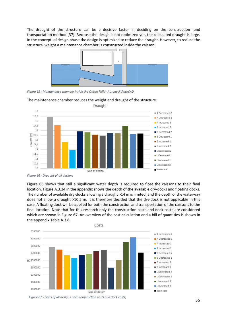
55

The draught of the structure can be a decisive factor in deciding on the construction- and transportation method [37]. Because the design is not optimized yet, the calculated draught is large. In the conceptual design phase the design is optimized to reduce the draught. However, to reduce the structural weight a maintenance chamber is constructed inside the caisson.

Figure 65 - Maintenance chamber inside the Ocean Falls - Autodesk AutoCAD

The maintenance chamber reduces the weight and draught of the structure.

Figure 66 - Draught of all designs

Figure 66 shows that still a significant water depth is required to float the caissons to their final location. Figure A.3.34 in the appendix shows the depth of the available dry-docks and floating docks. The number of available dry-docks allowing a draught >14 m is limited, and the depth of the waterway does not allow a draught >10.5 m. It is therefore decided that the dry-dock is not applicable in this case. A floating dock will be applied for both the construction and transportation of the caissons to the final location. Note that for this research only the construction costs and dock costs are considered which are shown in Figure 67. An overview of the cost calculation and a bill of quantities is shown in the appendix Table A.3.8.

Figure 67 - Costs of all designs (incl. construction costs and dock costs)

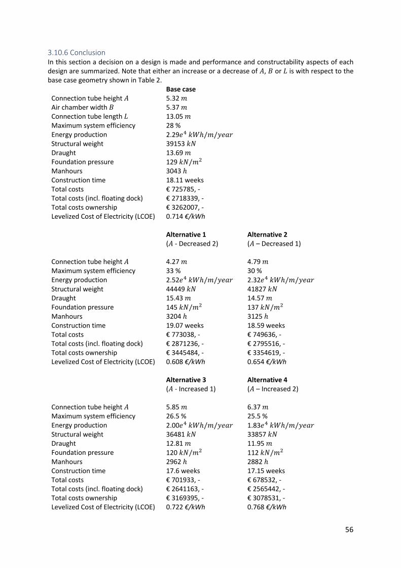
56

3.10.6 Conclusion In this section a decision on a design is made and performance and constructability aspects of each design are summarized. Note that either an increase or a decrease of 𝐴, 𝐵 or 𝐿 is with respect to the base case geometry shown in Table 2.

Base case Connection tube height 𝐴 5.32 𝑚 Air chamber width 𝐵 5.37 𝑚 Connection tube length 𝐿 13.05 𝑚 Maximum system efficiency 28 % Energy production 2.29𝑒4 𝑘𝑊ℎ/𝑚/𝑦𝑒𝑎𝑟 Structural weight 39153 𝑘𝑁 Draught 13.69 𝑚 Foundation pressure 129 𝑘𝑁/𝑚2 Manhours 3043 ℎ Construction time 18.11 weeks Total costs € 725785, - Total costs (incl. floating dock) € 2718339, - Total costs ownership € 3262007, - Levelized Cost of Electricity (LCOE) 0.714 €/kWh

Alternative 1

(𝐴 - Decreased 2) Alternative 2 (𝐴 – Decreased 1)

Connection tube height 𝐴 4.27 𝑚 4.79 𝑚 Maximum system efficiency 33 % 30 % Energy production 2.52𝑒4 𝑘𝑊ℎ/𝑚/𝑦𝑒𝑎𝑟 2.32𝑒4 𝑘𝑊ℎ/𝑚/𝑦𝑒𝑎𝑟 Structural weight 44449 𝑘𝑁 41827 𝑘𝑁 Draught 15.43 𝑚 14.57 𝑚 Foundation pressure 145 𝑘𝑁/𝑚2 137 𝑘𝑁/𝑚2 Manhours 3204 ℎ 3125 ℎ Construction time 19.07 weeks 18.59 weeks Total costs € 773038, - € 749636, - Total costs (incl. floating dock) € 2871236, - € 2795516, - Total costs ownership € 3445484, - € 3354619, - Levelized Cost of Electricity (LCOE) 0.608 €/kWh 0.654 €/kWh

Alternative 3

(𝐴 - Increased 1) Alternative 4 (𝐴 – Increased 2)

Connection tube height 𝐴 5.85 𝑚 6.37 𝑚 Maximum system efficiency 26.5 % 25.5 % Energy production 2.00𝑒4 𝑘𝑊ℎ/𝑚/𝑦𝑒𝑎𝑟 1.83𝑒4 𝑘𝑊ℎ/𝑚/𝑦𝑒𝑎𝑟 Structural weight 36481 𝑘𝑁 33857 𝑘𝑁 Draught 12.81 𝑚 11.95 𝑚 Foundation pressure 120 𝑘𝑁/𝑚2 112 𝑘𝑁/𝑚2 Manhours 2962 ℎ 2882 ℎ Construction time 17.6 weeks 17.15 weeks Total costs € 701933, - € 678532, - Total costs (incl. floating dock) € 2641163, - € 2565442, - Total costs ownership € 3169395, - € 3078531, - Levelized Cost of Electricity (LCOE) 0.722 €/kWh 0.768 €/kWh

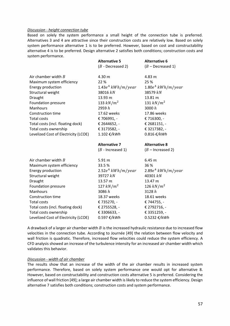
57

Discussion - height connection tube Based on solely the system performance a small height of the connection tube is preferred. Alternatives 3 and 4 are attractive since their construction costs are relatively low. Based on solely system performance alternative 1 is to be preferred. However, based on cost and constructability alternative 4 is to be preferred. Design alternative 2 satisfies both conditions; construction costs and system performance.

Alternative 5 (𝐵 - Decreased 2)

Alternative 6 (𝐵 – Decreased 1)

Air chamber width 𝐵 4.30 𝑚 4.83 𝑚 Maximum system efficiency 22 % 25 % Energy production 1.43𝑒4 𝑘𝑊ℎ/𝑚/𝑦𝑒𝑎𝑟 1.80𝑒4 𝑘𝑊ℎ/𝑚/𝑦𝑒𝑎𝑟 Structural weight 38016 𝑘𝑁 38579 𝑘𝑁 Draught 13.93 𝑚 13.81 𝑚 Foundation pressure 133 𝑘𝑁/𝑚2 131 𝑘𝑁/𝑚2 Manhours 2959 ℎ 3000 ℎ Construction time 17.62 weeks 17.86 weeks Total costs € 706991, - € 716300, - Total costs (incl. floating dock) € 2644652, - € 2681151, - Total costs ownership € 3173582, - € 3217382, - Levelized Cost of Electricity (LCOE) 1.102 €/kWh 0.816 €/kWh

Alternative 7

(𝐵 - Increased 1) Alternative 8 (𝐵 – Increased 2)

Air chamber width 𝐵 5.91 𝑚 6.45 𝑚 Maximum system efficiency 33.5 % 36 % Energy production 2.52𝑒4 𝑘𝑊ℎ/𝑚/𝑦𝑒𝑎𝑟 2.89𝑒4 𝑘𝑊ℎ/𝑚/𝑦𝑒𝑎𝑟 Structural weight 39727 𝑘𝑁 40301 𝑘𝑁 Draught 13.57 𝑚 13.47 𝑚 Foundation pressure 127 𝑘𝑁/𝑚2 126 𝑘𝑁/𝑚2 Manhours 3086 ℎ 3128 ℎ Construction time 18.37 weeks 18.61 weeks Total costs € 735270, - € 744755, - Total costs (incl. floating dock) € 2755528, - € 2792716, - Total costs ownership € 3306633, - € 3351259, - Levelized Cost of Electricity (LCOE) 0.597 €/kWh 0.5232 €/kWh

A drawback of a larger air chamber width 𝐵 is the increased hydraulic resistance due to increased flow velocities in the connection tube. According to Journée [49] the relation between flow velocity and wall friction is quadratic. Therefore, increased flow velocities could reduce the system efficiency. A CFD analysis showed an increase of the turbulence intensity for an increased air chamber width which validates this behavior. Discussion - width of air chamber The results show that an increase of the width of the air chamber results in increased system performance. Therefore, based on solely system performance one would opt for alternative 8. However, based on constructability and construction costs alternative 5 is preferred. Considering the influence of wall friction [49]; a large air chamber width is likely to reduce the system efficiency. Design alternative 7 satisfies both conditions; construction costs and system performance.

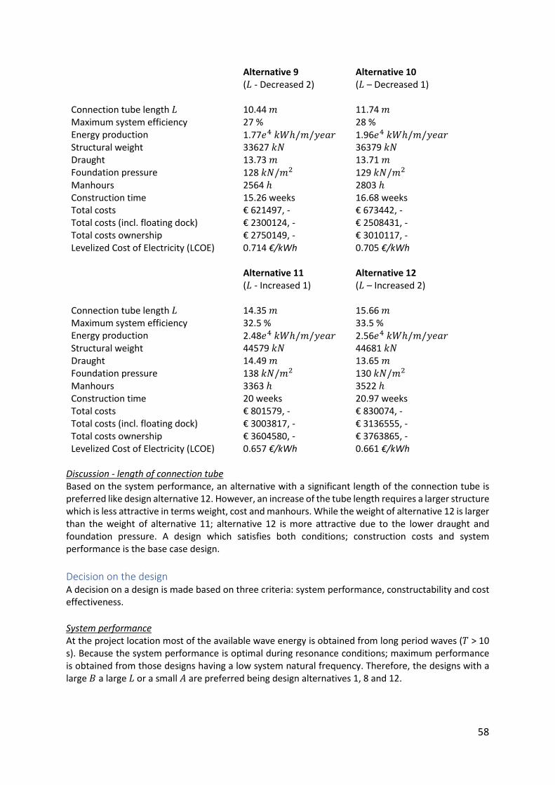
58

Alternative 9 (𝐿 - Decreased 2)

Alternative 10 (𝐿 – Decreased 1)

Connection tube length 𝐿 10.44 𝑚 11.74 𝑚 Maximum system efficiency 27 % 28 % Energy production 1.77𝑒4 𝑘𝑊ℎ/𝑚/𝑦𝑒𝑎𝑟 1.96𝑒4 𝑘𝑊ℎ/𝑚/𝑦𝑒𝑎𝑟 Structural weight 33627 𝑘𝑁 36379 𝑘𝑁 Draught 13.73 𝑚 13.71 𝑚 Foundation pressure 128 𝑘𝑁/𝑚2 129 𝑘𝑁/𝑚2 Manhours 2564 ℎ 2803 ℎ Construction time 15.26 weeks 16.68 weeks Total costs € 621497, - € 673442, - Total costs (incl. floating dock) € 2300124, - € 2508431, - Total costs ownership € 2750149, - € 3010117, - Levelized Cost of Electricity (LCOE) 0.714 €/kWh 0.705 €/kWh

Alternative 11

(𝐿 - Increased 1) Alternative 12 (𝐿 – Increased 2)

Connection tube length 𝐿 14.35 𝑚 15.66 𝑚 Maximum system efficiency 32.5 % 33.5 % Energy production 2.48𝑒4 𝑘𝑊ℎ/𝑚/𝑦𝑒𝑎𝑟 2.56𝑒4 𝑘𝑊ℎ/𝑚/𝑦𝑒𝑎𝑟 Structural weight 44579 𝑘𝑁 44681 𝑘𝑁 Draught 14.49 𝑚 13.65 𝑚 Foundation pressure 138 𝑘𝑁/𝑚2 130 𝑘𝑁/𝑚2 Manhours 3363 ℎ 3522 ℎ Construction time 20 weeks 20.97 weeks Total costs € 801579, - € 830074, - Total costs (incl. floating dock) € 3003817, - € 3136555, - Total costs ownership € 3604580, - € 3763865, - Levelized Cost of Electricity (LCOE) 0.657 €/kWh 0.661 €/kWh

Discussion - length of connection tube Based on the system performance, an alternative with a significant length of the connection tube is preferred like design alternative 12. However, an increase of the tube length requires a larger structure which is less attractive in terms weight, cost and manhours. While the weight of alternative 12 is larger than the weight of alternative 11; alternative 12 is more attractive due to the lower draught and foundation pressure. A design which satisfies both conditions; construction costs and system performance is the base case design.

Decision on the design A decision on a design is made based on three criteria: system performance, constructability and cost effectiveness.

System performance At the project location most of the available wave energy is obtained from long period waves (𝑇 > 10 s). Because the system performance is optimal during resonance conditions; maximum performance is obtained from those designs having a low system natural frequency. Therefore, the designs with a large 𝐵 a large 𝐿 or a small 𝐴 are preferred being design alternatives 1, 8 and 12.

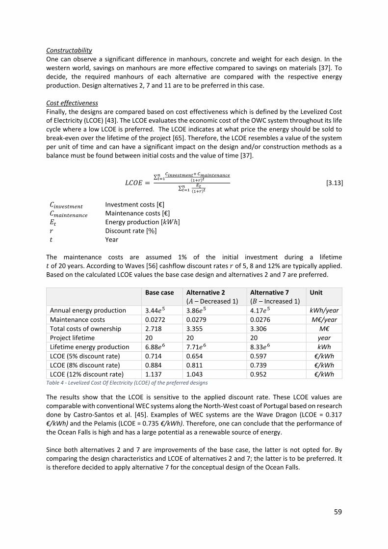
59

Constructability One can observe a significant difference in manhours, concrete and weight for each design. In the western world, savings on manhours are more effective compared to savings on materials [37]. To decide, the required manhours of each alternative are compared with the respective energy production. Design alternatives 2, 7 and 11 are to be preferred in this case. Cost effectiveness Finally, the designs are compared based on cost effectiveness which is defined by the Levelized Cost of Electricity (LCOE) [43]. The LCOE evaluates the economic cost of the OWC system throughout its life cycle where a low LCOE is preferred. The LCOE indicates at what price the energy should be sold to break-even over the lifetime of the project [65]. Therefore, the LCOE resembles a value of the system per unit of time and can have a significant impact on the design and/or construction methods as a balance must be found between initial costs and the value of time [37].

𝐶𝑖𝑛𝑣𝑒𝑠𝑡𝑚𝑒𝑛𝑡 Investment costs [€] 𝐶𝑚𝑎𝑖𝑛𝑡𝑒𝑛𝑎𝑛𝑐𝑒 Maintenance costs [€] 𝐸𝑡 Energy production [𝑘𝑊ℎ] 𝑟 Discount rate [%] 𝑡 Year

The maintenance costs are assumed 1% of the initial investment during a lifetime 𝑡 of 20 years. According to Waves [56] cashflow discount rates 𝑟 of 5, 8 and 12% are typically applied. Based on the calculated LCOE values the base case design and alternatives 2 and 7 are preferred.

Base case Alternative 2 (𝐴 – Decreased 1)

Alternative 7 (𝐵 – Increased 1)

Unit

Annual energy production 3.44𝑒5 3.86𝑒5 4.17𝑒5 kWh/year

Maintenance costs 0.0272 0.0279 0.0276 M€/year

Total costs of ownership 2.718 3.355 3.306 M€

Project lifetime 20 20 20 year

Lifetime energy production 6.88𝑒6 7.71𝑒6 8.33𝑒6 kWh

LCOE (5% discount rate) 0.714 0.654 0.597 €/kWh

LCOE (8% discount rate) 0.884 0.811 0.739 €/kWh

LCOE (12% discount rate) 1.137 1.043 0.952 €/kWh Table 4 - Levelized Cost Of Electricity (LCOE) of the preferred designs

The results show that the LCOE is sensitive to the applied discount rate. These LCOE values are comparable with conventional WEC systems along the North-West coast of Portugal based on research done by Castro-Santos et al. [45]. Examples of WEC systems are the Wave Dragon (LCOE = 0.317 €/kWh) and the Pelamis (LCOE = 0.735 €/kWh). Therefore, one can conclude that the performance of the Ocean Falls is high and has a large potential as a renewable source of energy. Since both alternatives 2 and 7 are improvements of the base case, the latter is not opted for. By comparing the design characteristics and LCOE of alternatives 2 and 7; the latter is to be preferred. It is therefore decided to apply alternative 7 for the conceptual design of the Ocean Falls.

𝐿𝐶𝑂𝐸 = ∑

𝐶𝑖𝑛𝑣𝑒𝑠𝑡𝑚𝑒𝑛𝑡+ 𝐶𝑚𝑎𝑖𝑛𝑡𝑒𝑛𝑎𝑛𝑐𝑒(1+𝑟)𝑡

𝑛𝑡=1

∑ 𝐸𝑡

(1+𝑟)𝑡𝑛𝑡=1

[3.13]

[2.2]

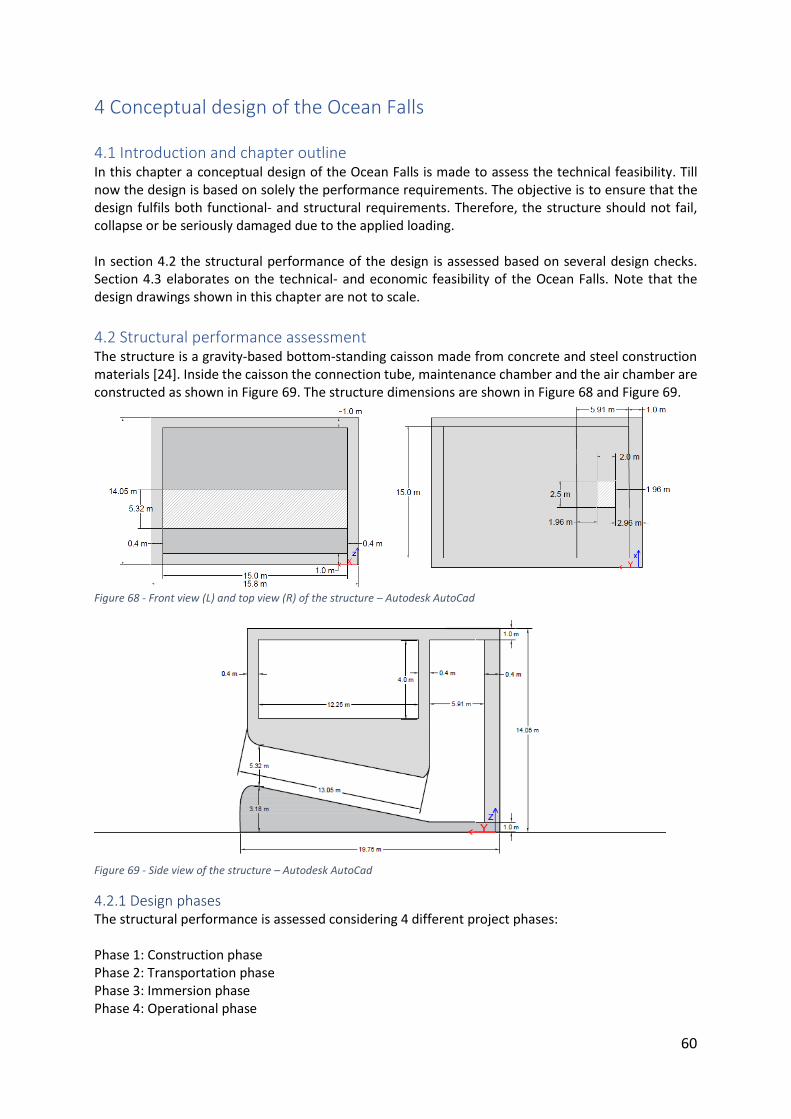
60

4 Conceptual design of the Ocean Falls

4.1 Introduction and chapter outline In this chapter a conceptual design of the Ocean Falls is made to assess the technical feasibility. Till now the design is based on solely the performance requirements. The objective is to ensure that the design fulfils both functional- and structural requirements. Therefore, the structure should not fail, collapse or be seriously damaged due to the applied loading. In section 4.2 the structural performance of the design is assessed based on several design checks. Section 4.3 elaborates on the technical- and economic feasibility of the Ocean Falls. Note that the design drawings shown in this chapter are not to scale.

4.2 Structural performance assessment The structure is a gravity-based bottom-standing caisson made from concrete and steel construction materials [24]. Inside the caisson the connection tube, maintenance chamber and the air chamber are constructed as shown in Figure 69. The structure dimensions are shown in Figure 68 and Figure 69.

Figure 68 - Front view (L) and top view (R) of the structure – Autodesk AutoCad

Figure 69 - Side view of the structure – Autodesk AutoCad

4.2.1 Design phases The structural performance is assessed considering 4 different project phases: Phase 1: Construction phase Phase 2: Transportation phase Phase 3: Immersion phase Phase 4: Operational phase

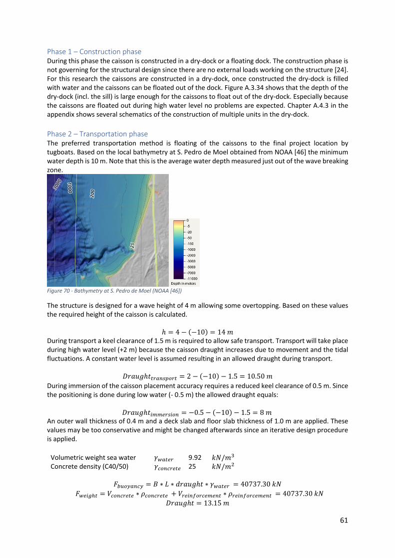
61

Phase 1 – Construction phase During this phase the caisson is constructed in a dry-dock or a floating dock. The construction phase is not governing for the structural design since there are no external loads working on the structure [24]. For this research the caissons are constructed in a dry-dock, once constructed the dry-dock is filled with water and the caissons can be floated out of the dock. Figure A.3.34 shows that the depth of the dry-dock (incl. the sill) is large enough for the caissons to float out of the dry-dock. Especially because the caissons are floated out during high water level no problems are expected. Chapter A.4.3 in the appendix shows several schematics of the construction of multiple units in the dry-dock.

Phase 2 – Transportation phase The preferred transportation method is floating of the caissons to the final project location by tugboats. Based on the local bathymetry at S. Pedro de Moel obtained from NOAA [46] the minimum water depth is 10 m. Note that this is the average water depth measured just out of the wave breaking zone.

Figure 70 - Bathymetry at S. Pedro de Moel (NOAA [46])

The structure is designed for a wave height of 4 m allowing some overtopping. Based on these values the required height of the caisson is calculated.

ℎ = 4 − (−10) = 14 𝑚 During transport a keel clearance of 1.5 m is required to allow safe transport. Transport will take place during high water level (+2 m) because the caisson draught increases due to movement and the tidal fluctuations. A constant water level is assumed resulting in an allowed draught during transport.

𝐷𝑟𝑎𝑢𝑔ℎ𝑡𝑡𝑟𝑎𝑛𝑠𝑝𝑜𝑟𝑡 = 2 − (−10) − 1.5 = 10.50 𝑚

During immersion of the caisson placement accuracy requires a reduced keel clearance of 0.5 m. Since the positioning is done during low water (- 0.5 m) the allowed draught equals:

𝐷𝑟𝑎𝑢𝑔ℎ𝑡𝑖𝑚𝑚𝑒𝑟𝑠𝑖𝑜𝑛 = −0.5 − (−10) − 1.5 = 8 𝑚 An outer wall thickness of 0.4 m and a deck slab and floor slab thickness of 1.0 m are applied. These values may be too conservative and might be changed afterwards since an iterative design procedure is applied.

Volumetric weight sea water 𝛾𝑤𝑎𝑡𝑒𝑟 9.92 𝑘𝑁/𝑚3 Concrete density (C40/50) 𝛾𝑐𝑜𝑛𝑐𝑟𝑒𝑡𝑒 25 𝑘𝑁/𝑚2

𝐹𝑏𝑢𝑜𝑦𝑎𝑛𝑐𝑦 = 𝐵 ∗ 𝐿 ∗ 𝑑𝑟𝑎𝑢𝑔ℎ𝑡 ∗ 𝛾𝑤𝑎𝑡𝑒𝑟 = 40737.30 𝑘𝑁

𝐹𝑤𝑒𝑖𝑔ℎ𝑡 = 𝑉𝑐𝑜𝑛𝑐𝑟𝑒𝑡𝑒 ∗ 𝜌𝑐𝑜𝑛𝑐𝑟𝑒𝑡𝑒 + 𝑉𝑟𝑒𝑖𝑛𝑓𝑜𝑟𝑐𝑒𝑚𝑒𝑛𝑡 ∗ 𝜌𝑟𝑒𝑖𝑛𝑓𝑜𝑟𝑐𝑒𝑚𝑒𝑛𝑡 = 40737.30 𝑘𝑁

𝐷𝑟𝑎𝑢𝑔ℎ𝑡 = 13.15 𝑚

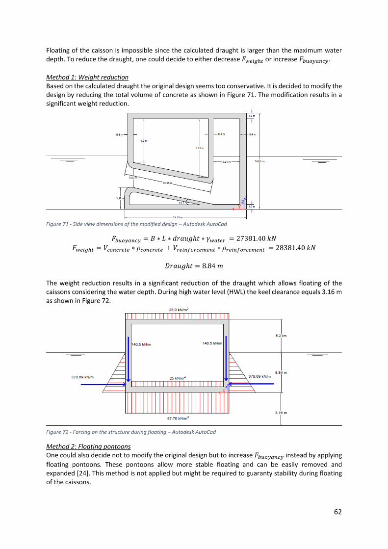
62

Floating of the caisson is impossible since the calculated draught is larger than the maximum water depth. To reduce the draught, one could decide to either decrease 𝐹𝑤𝑒𝑖𝑔ℎ𝑡 or increase 𝐹𝑏𝑢𝑜𝑦𝑎𝑛𝑐𝑦.

Method 1: Weight reduction Based on the calculated draught the original design seems too conservative. It is decided to modify the design by reducing the total volume of concrete as shown in Figure 71. The modification results in a significant weight reduction.

Figure 71 - Side view dimensions of the modified design – Autodesk AutoCad

𝐹𝑏𝑢𝑜𝑦𝑎𝑛𝑐𝑦 = 𝐵 ∗ 𝐿 ∗ 𝑑𝑟𝑎𝑢𝑔ℎ𝑡 ∗ 𝛾𝑤𝑎𝑡𝑒𝑟 = 27381.40 𝑘𝑁

𝐹𝑤𝑒𝑖𝑔ℎ𝑡 = 𝑉𝑐𝑜𝑛𝑐𝑟𝑒𝑡𝑒 ∗ 𝜌𝑐𝑜𝑛𝑐𝑟𝑒𝑡𝑒 + 𝑉𝑟𝑒𝑖𝑛𝑓𝑜𝑟𝑐𝑒𝑚𝑒𝑛𝑡 ∗ 𝜌𝑟𝑒𝑖𝑛𝑓𝑜𝑟𝑐𝑒𝑚𝑒𝑛𝑡 = 28381.40 𝑘𝑁

𝐷𝑟𝑎𝑢𝑔ℎ𝑡 = 8.84 𝑚

The weight reduction results in a significant reduction of the draught which allows floating of the caissons considering the water depth. During high water level (HWL) the keel clearance equals 3.16 m as shown in Figure 72.

Figure 72 - Forcing on the structure during floating – Autodesk AutoCad

Method 2: Floating pontoons One could also decide not to modify the original design but to increase 𝐹𝑏𝑢𝑜𝑦𝑎𝑛𝑐𝑦 instead by applying

floating pontoons. These pontoons allow more stable floating and can be easily removed and expanded [24]. This method is not applied but might be required to guaranty stability during floating of the caissons.

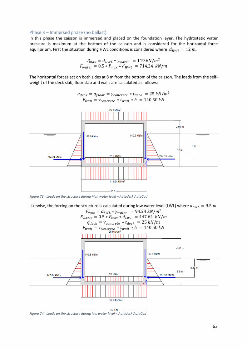
63

Phase 3 – Immersed phase (no ballast) In this phase the caisson is immersed and placed on the foundation layer. The hydrostatic water pressure is maximum at the bottom of the caisson and is considered for the horizontal force equilibrium. First the situation during HWL conditions is considered where 𝑑𝐻𝑊𝐿 = 12 𝑚.

𝑃𝑚𝑎𝑥 = 𝑑𝐻𝑊𝐿 ∗ 𝛾𝑤𝑎𝑡𝑒𝑟 = 119 𝑘𝑁/𝑚2 𝐹𝑤𝑎𝑡𝑒𝑟 = 0.5 ∗ 𝑃𝑚𝑎𝑥 ∗ 𝑑𝐻𝑊𝐿 = 714.24 𝑘𝑁/𝑚

The horizontal forces act on both sides at 8 m from the bottom of the caisson. The loads from the self-weight of the deck slab, floor slab and walls are calculated as follows:

𝑞𝑑𝑒𝑐𝑘 = 𝑞𝑓𝑙𝑜𝑜𝑟 = 𝛾𝑐𝑜𝑛𝑐𝑟𝑒𝑡𝑒 ∗ 𝑡𝑑𝑒𝑐𝑘 = 25 𝑘𝑁/𝑚2

𝐹𝑤𝑎𝑙𝑙 = 𝛾𝑐𝑜𝑛𝑐𝑟𝑒𝑡𝑒 ∗ 𝑡𝑤𝑎𝑙𝑙 ∗ ℎ = 140.50 𝑘𝑁

Figure 73 - Loads on the structure during high water level – Autodesk AutoCad

Likewise, the forcing on the structure is calculated during low water level (LWL) where 𝑑𝐿𝑊𝐿 = 9.5 𝑚. 𝑃𝑚𝑎𝑥 = 𝑑𝐿𝑊𝐿 ∗ 𝛾𝑤𝑎𝑡𝑒𝑟 = 94.24 𝑘𝑁/𝑚2

𝐹𝑤𝑎𝑡𝑒𝑟 = 0.5 ∗ 𝑃𝑚𝑎𝑥 ∗ 𝑑𝐿𝑊𝐿 = 447.64 𝑘𝑁/𝑚 𝑞𝑑𝑒𝑐𝑘 = 𝛾𝑐𝑜𝑛𝑐𝑟𝑒𝑡𝑒 ∗ 𝑡𝑑𝑒𝑐𝑘 = 25 𝑘𝑁/𝑚

𝐹𝑤𝑎𝑙𝑙 = 𝛾𝑐𝑜𝑛𝑐𝑟𝑒𝑡𝑒 ∗ 𝑡𝑤𝑎𝑙𝑙 ∗ ℎ = 140.50 𝑘𝑁

Figure 74 - Loads on the structure during low water level – Autodesk AutoCad

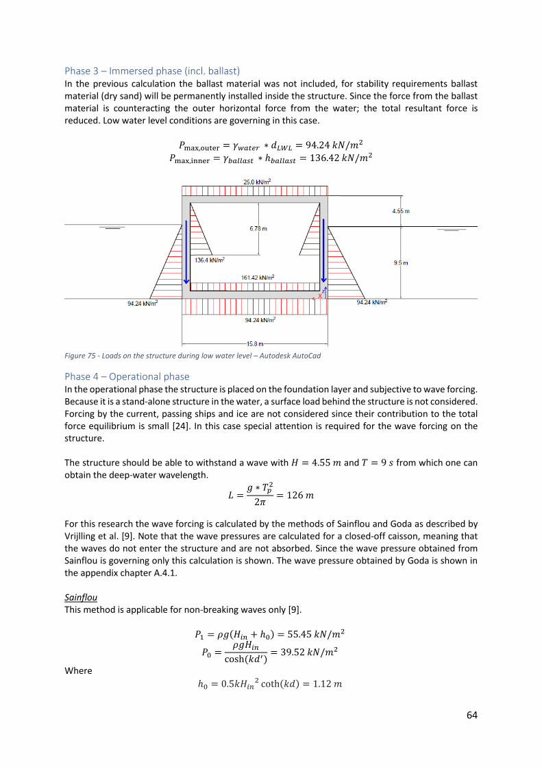
64

Phase 3 – Immersed phase (incl. ballast) In the previous calculation the ballast material was not included, for stability requirements ballast material (dry sand) will be permanently installed inside the structure. Since the force from the ballast material is counteracting the outer horizontal force from the water; the total resultant force is reduced. Low water level conditions are governing in this case.

𝑃max,outer = 𝛾𝑤𝑎𝑡𝑒𝑟 ∗ 𝑑𝐿𝑊𝐿 = 94.24 𝑘𝑁/𝑚2

𝑃max,inner = 𝛾𝑏𝑎𝑙𝑙𝑎𝑠𝑡 ∗ ℎ𝑏𝑎𝑙𝑙𝑎𝑠𝑡 = 136.42 𝑘𝑁/𝑚2

Figure 75 - Loads on the structure during low water level – Autodesk AutoCad

Phase 4 – Operational phase In the operational phase the structure is placed on the foundation layer and subjective to wave forcing. Because it is a stand-alone structure in the water, a surface load behind the structure is not considered. Forcing by the current, passing ships and ice are not considered since their contribution to the total force equilibrium is small [24]. In this case special attention is required for the wave forcing on the structure. The structure should be able to withstand a wave with 𝐻 = 4.55 𝑚 and 𝑇 = 9 𝑠 from which one can obtain the deep-water wavelength.

𝐿 =𝑔 ∗ 𝑇𝑝

2

2𝜋= 126 𝑚

For this research the wave forcing is calculated by the methods of Sainflou and Goda as described by Vrijlling et al. [9]. Note that the wave pressures are calculated for a closed-off caisson, meaning that the waves do not enter the structure and are not absorbed. Since the wave pressure obtained from Sainflou is governing only this calculation is shown. The wave pressure obtained by Goda is shown in the appendix chapter A.4.1. Sainflou This method is applicable for non-breaking waves only [9].

𝑃1 = 𝜌𝑔(𝐻𝑖𝑛 + ℎ0) = 55.45 𝑘𝑁/𝑚2

𝑃0 =𝜌𝑔𝐻𝑖𝑛

cosh (𝑘𝑑′)= 39.52 𝑘𝑁/𝑚2

Where

ℎ0 = 0.5𝑘𝐻𝑖𝑛2 coth(𝑘𝑑) = 1.12 𝑚

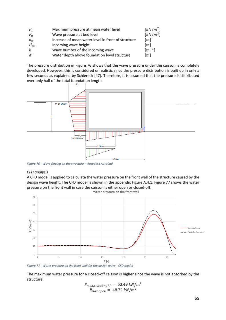
65

𝑃1 Maximum pressure at mean water level [𝑘𝑁/𝑚2] 𝑃0 Wave pressure at bed level [𝑘𝑁/𝑚2] ℎ0 Increase of mean water level in front of structure [𝑚] 𝐻𝑖𝑛 Incoming wave height [𝑚] 𝑘 Wave number of the incoming wave [𝑚−1] 𝑑′ Water depth above foundation level structure [𝑚]

The pressure distribution in Figure 76 shows that the wave pressure under the caisson is completely developed. However, this is considered unrealistic since the pressure distribution is built up in only a few seconds as explained by Schiereck [47]. Therefore, it is assumed that the pressure is distributed over only half of the total foundation length.

Figure 76 - Wave forcing on the structure – Autodesk AutoCad

CFD analysis A CFD model is applied to calculate the water pressure on the front wall of the structure caused by the design wave height. The CFD model is shown in the appendix Figure A.4.1. Figure 77 shows the water pressure on the front wall in case the caisson is either open or closed-off.

Figure 77 - Water pressure on the front wall for the design wave - CFD model

The maximum water pressure for a closed-off caisson is higher since the wave is not absorbed by the structure.

𝑃𝑚𝑎𝑥,𝑐𝑙𝑜𝑠𝑒𝑑−𝑜𝑓𝑓 = 53.49 𝑘𝑁/𝑚2

𝑃𝑚𝑎𝑥,𝑜𝑝𝑒𝑛 = 48.72 𝑘𝑁/𝑚2

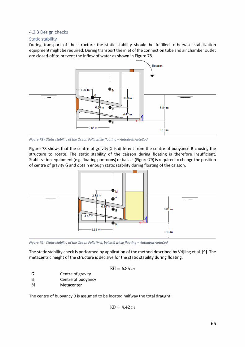
66

4.2.3 Design checks

Static stability During transport of the structure the static stability should be fulfilled, otherwise stabilization equipment might be required. During transport the inlet of the connection tube and air chamber outlet are closed-off to prevent the inflow of water as shown in Figure 78.

Figure 78 - Static stability of the Ocean Falls while floating – Autodesk AutoCad

Figure 78 shows that the centre of gravity G is different from the centre of buoyance B causing the structure to rotate. The static stability of the caisson during floating is therefore insufficient. Stabilization equipment (e.g. floating pontoons) or ballast (Figure 79) is required to change the position of centre of gravity G and obtain enough static stability during floating of the caisson.

Figure 79 - Static stability of the Ocean Falls (incl. ballast) while floating – Autodesk AutoCad

The static stability check is performed by application of the method described by Vrijling et al. [9]. The metacentric height of the structure is decisive for the static stability during floating.

KG = 6.85 𝑚 G Centre of gravity B Centre of buoyancy M Metacenter

The centre of buoyancy B is assumed to be located halfway the total draught.

KB = 4.42 𝑚

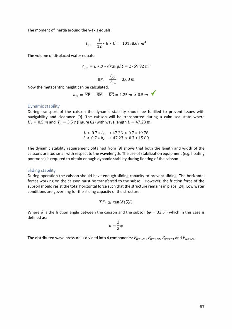
67

The moment of inertia around the y-axis equals:

𝐼𝑦𝑦 =1

12∗ 𝐵 ∗ 𝐿3 = 10158.67 𝑚4

The volume of displaced water equals:

𝑉𝑑𝑤 = 𝐿 ∗ 𝐵 ∗ 𝑑𝑟𝑎𝑢𝑔ℎ𝑡 = 2759.92 𝑚3

BM =𝐼𝑦𝑦

𝑉𝑑𝑤= 3.68 𝑚

Now the metacentric height can be calculated.

ℎ𝑚 = KB + BM − KG = 1.25 𝑚 > 0.5 𝑚

Dynamic stability During transport of the caisson the dynamic stability should be fulfilled to prevent issues with navigability and clearance [9]. The caisson will be transported during a calm sea state where 𝐻𝑠 = 0.5 𝑚 and 𝑇𝑝 = 5.5 𝑠 (Figure 62) with wave length 𝐿 = 47.23 𝑚.

𝐿 < 0.7 ∗ 𝑙𝑒 → 47.23 > 0.7 ∗ 19.76 𝐿 < 0.7 ∗ 𝑏𝑒 → 47.23 > 0.7 ∗ 15.80

The dynamic stability requirement obtained from [9] shows that both the length and width of the caissons are too small with respect to the wavelength. The use of stabilization equipment (e.g. floating pontoons) is required to obtain enough dynamic stability during floating of the caisson.

Sliding stability During operation the caisson should have enough sliding capacity to prevent sliding. The horizontal forces working on the caisson must be transferred to the subsoil. However, the friction force of the subsoil should resist the total horizontal force such that the structure remains in place [24]. Low water conditions are governing for the sliding capacity of the structure.

∑𝐹ℎ ≤ tan(𝛿) ∑𝐹𝑣 Where 𝛿 is the friction angle between the caisson and the subsoil (𝜑 = 32.5°) which in this case is defined as:

𝛿 =2

3𝜑

The distributed wave pressure is divided into 4 components: 𝐹𝑤𝑎𝑣𝑒1, 𝐹𝑤𝑎𝑣𝑒2, 𝐹𝑤𝑎𝑣𝑒3 and 𝐹𝑤𝑎𝑣𝑒4.

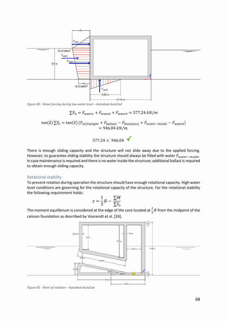
68

Figure 80 - Wave forcing during low water level – Autodesk AutoCad

∑𝐹ℎ = 𝐹𝑤𝑎𝑣𝑒1 + 𝐹𝑤𝑎𝑣𝑒2 + 𝐹𝑤𝑎𝑣𝑒3 = 577.24 𝑘𝑁/𝑚

tan(𝛿) ∑𝐹𝑣 = tan(𝛿) (𝐹𝑠𝑒𝑙𝑓𝑤𝑒𝑖𝑔ℎ𝑡 + 𝐹𝑏𝑎𝑙𝑙𝑎𝑠𝑡 − 𝐹𝑏𝑢𝑜𝑦𝑎𝑛𝑐𝑦 + 𝐹𝑤𝑎𝑡𝑒𝑟−𝑖𝑛𝑠𝑖𝑑𝑒 − 𝐹𝑤𝑎𝑣𝑒4)

= 946.04 𝑘𝑁/𝑚

577.24 < 946.04 There is enough sliding capacity and the structure will not slide away due to the applied forcing. However, to guarantee sliding stability the structure should always be filled with water 𝐹𝑤𝑎𝑡𝑒𝑟−𝑖𝑛𝑠𝑖𝑑𝑒. In case maintenance is required and there is no water inside the structure; additional ballast is required to obtain enough sliding capacity.

Rotational stability To prevent rotation during operation the structure should have enough rotational capacity. High water level conditions are governing for the rotational capacity of the structure. For the rotational stability the following requirement holds:

𝑧 =1

3𝐵 −

∑𝑀

∑𝐹𝑣

The moment equilibrium is considered at the edge of the core located at 1

3𝐵 from the midpoint of the

caisson foundation as described by Voorendt et al. [24].

Figure 81 - Point of rotation – Autodesk AutoCad

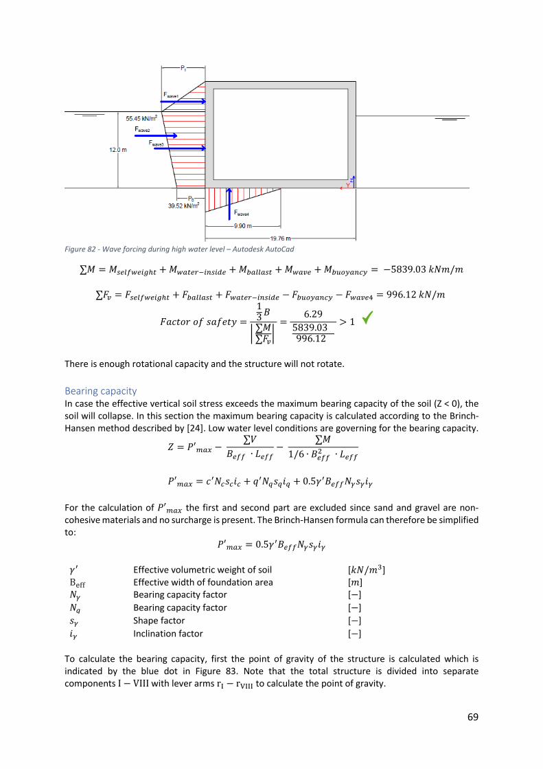
69

Figure 82 - Wave forcing during high water level – Autodesk AutoCad

∑𝑀 = 𝑀𝑠𝑒𝑙𝑓𝑤𝑒𝑖𝑔ℎ𝑡 + 𝑀𝑤𝑎𝑡𝑒𝑟−𝑖𝑛𝑠𝑖𝑑𝑒 + 𝑀𝑏𝑎𝑙𝑙𝑎𝑠𝑡 + 𝑀𝑤𝑎𝑣𝑒 + 𝑀𝑏𝑢𝑜𝑦𝑎𝑛𝑐𝑦 = −5839.03 𝑘𝑁𝑚/𝑚

∑𝐹𝑣 = 𝐹𝑠𝑒𝑙𝑓𝑤𝑒𝑖𝑔ℎ𝑡 + 𝐹𝑏𝑎𝑙𝑙𝑎𝑠𝑡 + 𝐹𝑤𝑎𝑡𝑒𝑟−𝑖𝑛𝑠𝑖𝑑𝑒 − 𝐹𝑏𝑢𝑜𝑦𝑎𝑛𝑐𝑦 − 𝐹𝑤𝑎𝑣𝑒4 = 996.12 𝑘𝑁/𝑚

𝐹𝑎𝑐𝑡𝑜𝑟 𝑜𝑓 𝑠𝑎𝑓𝑒𝑡𝑦 =

13

𝐵

| ∑𝑀∑𝐹𝑣

| =

6.29

5839.03 996.12

> 1

There is enough rotational capacity and the structure will not rotate.

Bearing capacity In case the effective vertical soil stress exceeds the maximum bearing capacity of the soil (Z < 0), the soil will collapse. In this section the maximum bearing capacity is calculated according to the Brinch-Hansen method described by [24]. Low water level conditions are governing for the bearing capacity.

𝑍 = 𝑃′𝑚𝑎𝑥 − ∑𝑉

𝐵𝑒𝑓𝑓 ∙ 𝐿𝑒𝑓𝑓−

∑𝑀

1/6 ∙ 𝐵𝑒𝑓𝑓2 ∙ 𝐿𝑒𝑓𝑓

𝑃′𝑚𝑎𝑥 = 𝑐′𝑁𝑐𝑠𝑐𝑖𝑐 + 𝑞′𝑁𝑞𝑠𝑞𝑖𝑞 + 0.5𝛾′𝐵𝑒𝑓𝑓𝑁𝛾𝑠𝛾𝑖𝛾

For the calculation of 𝑃′𝑚𝑎𝑥 the first and second part are excluded since sand and gravel are non-cohesive materials and no surcharge is present. The Brinch-Hansen formula can therefore be simplified to:

𝑃′𝑚𝑎𝑥 = 0.5𝛾′𝐵𝑒𝑓𝑓𝑁𝛾𝑠𝛾𝑖𝛾

𝛾′ Effective volumetric weight of soil [𝑘𝑁/𝑚3] Beff Effective width of foundation area [𝑚] 𝑁𝛾 Bearing capacity factor [−]

𝑁𝑞 Bearing capacity factor [−]

𝑠𝛾 Shape factor [−]

𝑖𝛾 Inclination factor [−]

To calculate the bearing capacity, first the point of gravity of the structure is calculated which is indicated by the blue dot in Figure 83. Note that the total structure is divided into separate components I − VIII with lever arms rI − rVIII to calculate the point of gravity.

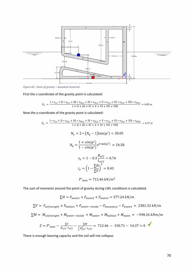
70

Figure 83 - Point of gravity – Autodesk AutoCad

First the z-coordinate of the gravity point is calculated:

𝐺𝑧 = I ∗ rI,z + II ∗ rII,z + III ∗ rIII,z + IV ∗ rIV,z + V ∗ rV,z + VI ∗ rVI,z + VII ∗ rVII,z

I + II + III + IV + V + VI + VII + VIII = 6.85 𝑚

Now the y-coordinate of the gravity point is calculated:

𝐺𝑧 = I ∗ rI,y + II ∗ rII,y + III ∗ rIII,y + IV ∗ rIV,y + V ∗ rV,y + VI ∗ rVI,y + VII ∗ rVII,y

I + II + III + IV + V + VI + VII + VIII = 6.37 𝑚

𝑁𝛾 = 2 ∗ (𝑁𝑞 − 1)tan (𝜑′) = 30.05

𝑁𝑞 =1 + 𝑠𝑖𝑛(𝜑′)

1 − 𝑠𝑖𝑛(𝜑′)eπ tan(𝜑′) = 24.58

𝑠𝛾 = 1 − 0.3𝐵𝑒𝑓𝑓

𝐿𝑒𝑓𝑓= 0.76

𝑖𝛾 = (1 −∑𝐻

∑𝑉)

3

= 0.43

𝑃′𝑚𝑎𝑥 = 712.46 𝑘𝑁/𝑚2

The sum of moments around the point of gravity during LWL conditions is calculated.

∑𝐻 = 𝐹𝑤𝑎𝑣𝑒1 + 𝐹𝑤𝑎𝑣𝑒2 + 𝐹𝑤𝑎𝑣𝑒3 = 577.24 𝑘𝑁/𝑚

∑𝑉 = 𝐹𝑠𝑒𝑙𝑓𝑤𝑒𝑖𝑔ℎ𝑡 + 𝐹𝑏𝑎𝑙𝑙𝑎𝑠𝑡 + 𝐹𝑤𝑎𝑡𝑒𝑟−𝑖𝑛𝑠𝑖𝑑𝑒 − 𝐹𝑏𝑢𝑜𝑦𝑎𝑛𝑐𝑦 − 𝐹𝑤𝑎𝑣𝑒4 = 2381.32 𝑘𝑁/𝑚

∑𝑀 = 𝑀𝑠𝑒𝑙𝑓𝑤𝑒𝑖𝑔ℎ𝑡 + 𝑀𝑤𝑎𝑡𝑒𝑟−𝑖𝑛𝑠𝑖𝑑𝑒 + 𝑀𝑤𝑎𝑡𝑒𝑟 + 𝑀𝑏𝑎𝑙𝑙𝑎𝑠𝑡 + 𝑀𝑤𝑎𝑣𝑒 = −598.16 𝑘𝑁𝑚/𝑚

𝑍 = 𝑃′𝑚𝑎𝑥 − ∑𝑉

𝐵𝑒𝑓𝑓 ∙𝐿𝑒𝑓𝑓−

∑𝑀1

6∙𝐵𝑒𝑓𝑓

2 ∙𝐿𝑒𝑓𝑓

= 712.46 − 150.71 − 14.37 > 0

There is enough bearing capacity and the soil will not collapse.

71

Scour protection During operation the structure is constantly loaded by waves and scour can be expected in front of the structure. According to Vrijling [9] a significant scour depth can result in geotechnical stability problems. To calculate the scour depth the method described by Schiereck et al. [47] and Breuser [9] is applied.

ℎ𝑠𝑐𝑜𝑢𝑟

ℎ0=

(0.5 ∗ 𝛼 ∗ 𝑢) − 𝑢𝑐

𝑢𝑐

ℎ0 (Initial) water depth [𝑚] 𝑢 Depth-averaged flow velocity [𝑚/𝑠] 𝑢𝑐 Critical velocity of particle motion [𝑚/𝑠] 𝛼 Turbulence coefficient [−]

The critical velocity of particle motion is calculated by applying the Shields equation.

𝑢𝑐 = 𝐶√𝛹𝑐 ∆𝐷𝑛50 = 1.22 𝑚/𝑠

𝐶 Chézy coefficient = 50 √𝑚/𝑠 𝐷𝑛50 Nominal diameter of sand particles = 0.0075 𝑚 ∆ Relative density = 1.59 𝛹𝑐 Shields parameter = 0.05

The shields parameter 𝛹𝑐 depends on the grain diameter 𝑑∗:

𝑑∗ = 𝐷50 √∆𝑔

𝑣2

3

𝑣 Kinematic viscosity = 1.33𝑒−6 𝑚2/𝑠 𝐷50 Diameter of sand particles = 0.0075 𝑚

This results in a scour depth ℎ𝑠𝑐𝑜𝑢𝑟 of 1.89 m from which the required length of the bed protection is obtained.

𝐿𝑏𝑝 = 𝛾𝑠𝑎𝑓𝑒𝑡𝑦 ∗ 𝑛𝑠 ∗ ℎ𝑠𝑐𝑜𝑢𝑟 = 11.31 𝑚

𝛾𝑠𝑎𝑓𝑒𝑡𝑦 Safety factor = 1.0

𝑛𝑠 1: 𝑛𝑠 is the average slope of the slide = 6 𝑚 (densely packed sand)

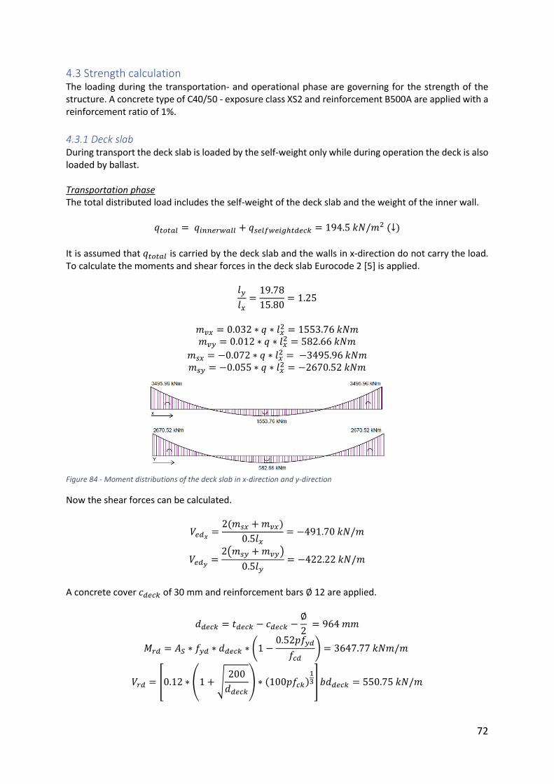
72

4.3 Strength calculation The loading during the transportation- and operational phase are governing for the strength of the structure. A concrete type of C40/50 - exposure class XS2 and reinforcement B500A are applied with a reinforcement ratio of 1%.

4.3.1 Deck slab During transport the deck slab is loaded by the self-weight only while during operation the deck is also loaded by ballast. Transportation phase The total distributed load includes the self-weight of the deck slab and the weight of the inner wall.

𝑞𝑡𝑜𝑡𝑎𝑙 = 𝑞𝑖𝑛𝑛𝑒𝑟𝑤𝑎𝑙𝑙 + 𝑞𝑠𝑒𝑙𝑓𝑤𝑒𝑖𝑔ℎ𝑡𝑑𝑒𝑐𝑘 = 194.5 𝑘𝑁/𝑚2 (↓)

It is assumed that 𝑞𝑡𝑜𝑡𝑎𝑙 is carried by the deck slab and the walls in x-direction do not carry the load. To calculate the moments and shear forces in the deck slab Eurocode 2 [5] is applied.

𝑙𝑦

𝑙𝑥=

19.78

15.80= 1.25

𝑚𝑣𝑥 = 0.032 ∗ 𝑞 ∗ 𝑙𝑥2 = 1553.76 𝑘𝑁𝑚

𝑚𝑣𝑦 = 0.012 ∗ 𝑞 ∗ 𝑙𝑥2 = 582.66 𝑘𝑁𝑚

𝑚𝑠𝑥 = −0.072 ∗ 𝑞 ∗ 𝑙𝑥2 = −3495.96 𝑘𝑁𝑚

𝑚𝑠𝑦 = −0.055 ∗ 𝑞 ∗ 𝑙𝑥2 = −2670.52 𝑘𝑁𝑚

Figure 84 - Moment distributions of the deck slab in x-direction and y-direction

Now the shear forces can be calculated.

𝑉𝑒𝑑𝑥=

2(𝑚𝑠𝑥 + 𝑚𝑣𝑥)

0.5𝑙𝑥= −491.70 𝑘𝑁/𝑚

𝑉𝑒𝑑𝑦=

2(𝑚𝑠𝑦 + 𝑚𝑣𝑦)

0.5𝑙𝑦= −422.22 𝑘𝑁/𝑚

A concrete cover 𝑐𝑑𝑒𝑐𝑘 of 30 mm and reinforcement bars ∅ 12 are applied.

𝑑𝑑𝑒𝑐𝑘 = 𝑡𝑑𝑒𝑐𝑘 − 𝑐𝑑𝑒𝑐𝑘 −∅

2 = 964 𝑚𝑚

𝑀𝑟𝑑 = 𝐴𝑆 ∗ 𝑓𝑦𝑑 ∗ 𝑑𝑑𝑒𝑐𝑘 ∗ (1 −0.52𝑝𝑓𝑦𝑑

𝑓𝑐𝑑) = 3647.77 𝑘𝑁𝑚/𝑚

𝑉𝑟𝑑 = [0.12 ∗ (1 + √200

𝑑𝑑𝑒𝑐𝑘) ∗ (100𝑝𝑓𝑐𝑘)

13] 𝑏𝑑𝑑𝑒𝑐𝑘 = 550.75 𝑘𝑁/𝑚

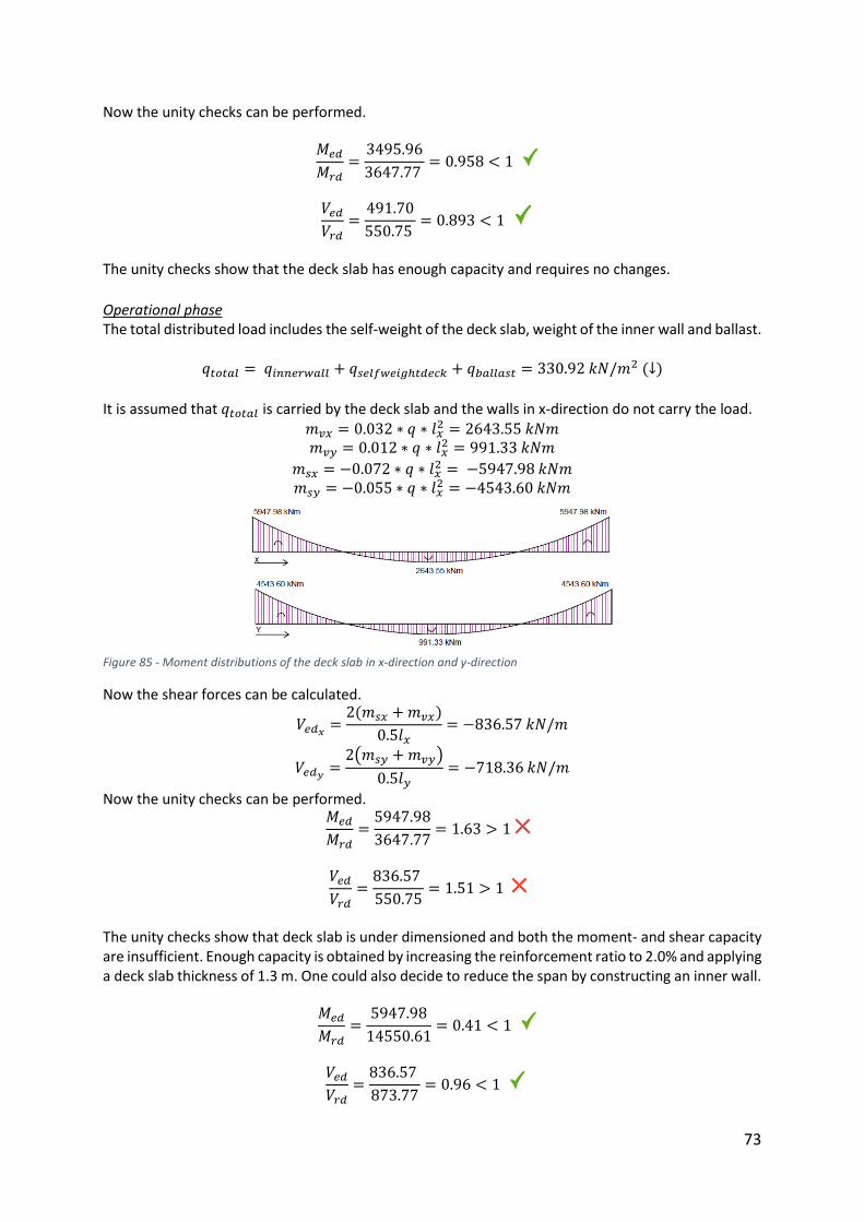
73

Now the unity checks can be performed.

𝑀𝑒𝑑

𝑀𝑟𝑑=

3495.96

3647.77 = 0.958 < 1

𝑉𝑒𝑑

𝑉𝑟𝑑=

491.70

550.75 = 0.893 < 1

The unity checks show that the deck slab has enough capacity and requires no changes.

Operational phase The total distributed load includes the self-weight of the deck slab, weight of the inner wall and ballast.

𝑞𝑡𝑜𝑡𝑎𝑙 = 𝑞𝑖𝑛𝑛𝑒𝑟𝑤𝑎𝑙𝑙 + 𝑞𝑠𝑒𝑙𝑓𝑤𝑒𝑖𝑔ℎ𝑡𝑑𝑒𝑐𝑘 + 𝑞𝑏𝑎𝑙𝑙𝑎𝑠𝑡 = 330.92 𝑘𝑁/𝑚2 (↓)

It is assumed that 𝑞𝑡𝑜𝑡𝑎𝑙 is carried by the deck slab and the walls in x-direction do not carry the load.

𝑚𝑣𝑥 = 0.032 ∗ 𝑞 ∗ 𝑙𝑥2 = 2643.55 𝑘𝑁𝑚

𝑚𝑣𝑦 = 0.012 ∗ 𝑞 ∗ 𝑙𝑥2 = 991.33 𝑘𝑁𝑚

𝑚𝑠𝑥 = −0.072 ∗ 𝑞 ∗ 𝑙𝑥2 = −5947.98 𝑘𝑁𝑚

𝑚𝑠𝑦 = −0.055 ∗ 𝑞 ∗ 𝑙𝑥2 = −4543.60 𝑘𝑁𝑚

Figure 85 - Moment distributions of the deck slab in x-direction and y-direction

Now the shear forces can be calculated.

𝑉𝑒𝑑𝑥=

2(𝑚𝑠𝑥 + 𝑚𝑣𝑥)

0.5𝑙𝑥= −836.57 𝑘𝑁/𝑚

𝑉𝑒𝑑𝑦=

2(𝑚𝑠𝑦 + 𝑚𝑣𝑦)

0.5𝑙𝑦= −718.36 𝑘𝑁/𝑚

Now the unity checks can be performed. 𝑀𝑒𝑑

𝑀𝑟𝑑=

5947.98

3647.77= 1.63 > 1

𝑉𝑒𝑑

𝑉𝑟𝑑=

836.57

550.75= 1.51 > 1

The unity checks show that deck slab is under dimensioned and both the moment- and shear capacity are insufficient. Enough capacity is obtained by increasing the reinforcement ratio to 2.0% and applying a deck slab thickness of 1.3 m. One could also decide to reduce the span by constructing an inner wall.

𝑀𝑒𝑑

𝑀𝑟𝑑=

5947.98

14550.61= 0.41 < 1

𝑉𝑒𝑑

𝑉𝑟𝑑=

836.57

873.77= 0.96 < 1

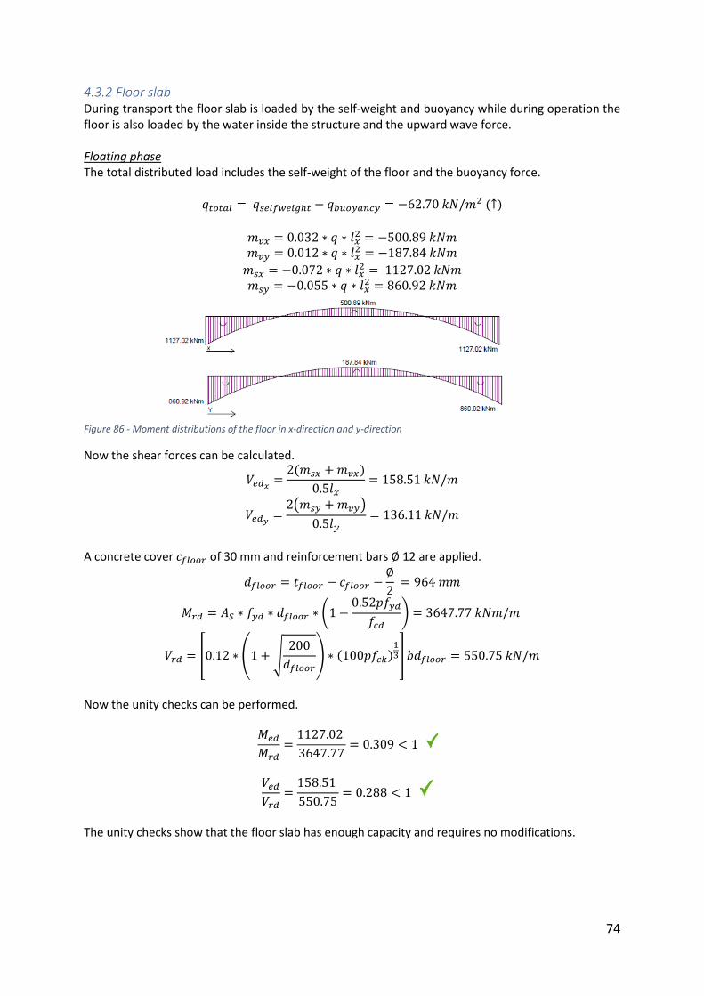
74

4.3.2 Floor slab During transport the floor slab is loaded by the self-weight and buoyancy while during operation the floor is also loaded by the water inside the structure and the upward wave force. Floating phase The total distributed load includes the self-weight of the floor and the buoyancy force.

𝑞𝑡𝑜𝑡𝑎𝑙 = 𝑞𝑠𝑒𝑙𝑓𝑤𝑒𝑖𝑔ℎ𝑡 − 𝑞𝑏𝑢𝑜𝑦𝑎𝑛𝑐𝑦 = −62.70 𝑘𝑁/𝑚2 (↑)

𝑚𝑣𝑥 = 0.032 ∗ 𝑞 ∗ 𝑙𝑥

2 = −500.89 𝑘𝑁𝑚 𝑚𝑣𝑦 = 0.012 ∗ 𝑞 ∗ 𝑙𝑥

2 = −187.84 𝑘𝑁𝑚

𝑚𝑠𝑥 = −0.072 ∗ 𝑞 ∗ 𝑙𝑥2 = 1127.02 𝑘𝑁𝑚

𝑚𝑠𝑦 = −0.055 ∗ 𝑞 ∗ 𝑙𝑥2 = 860.92 𝑘𝑁𝑚

Figure 86 - Moment distributions of the floor in x-direction and y-direction

Now the shear forces can be calculated.

𝑉𝑒𝑑𝑥=

2(𝑚𝑠𝑥 + 𝑚𝑣𝑥)

0.5𝑙𝑥= 158.51 𝑘𝑁/𝑚

𝑉𝑒𝑑𝑦=

2(𝑚𝑠𝑦 + 𝑚𝑣𝑦)

0.5𝑙𝑦= 136.11 𝑘𝑁/𝑚

A concrete cover 𝑐𝑓𝑙𝑜𝑜𝑟 of 30 mm and reinforcement bars ∅ 12 are applied.

𝑑𝑓𝑙𝑜𝑜𝑟 = 𝑡𝑓𝑙𝑜𝑜𝑟 − 𝑐𝑓𝑙𝑜𝑜𝑟 −∅

2 = 964 𝑚𝑚

𝑀𝑟𝑑 = 𝐴𝑆 ∗ 𝑓𝑦𝑑 ∗ 𝑑𝑓𝑙𝑜𝑜𝑟 ∗ (1 −0.52𝑝𝑓𝑦𝑑

𝑓𝑐𝑑) = 3647.77 𝑘𝑁𝑚/𝑚

𝑉𝑟𝑑 = [0.12 ∗ (1 + √200

𝑑𝑓𝑙𝑜𝑜𝑟) ∗ (100𝑝𝑓𝑐𝑘)

13] 𝑏𝑑𝑓𝑙𝑜𝑜𝑟 = 550.75 𝑘𝑁/𝑚

Now the unity checks can be performed.

𝑀𝑒𝑑

𝑀𝑟𝑑=

1127.02

3647.77= 0.309 < 1

𝑉𝑒𝑑

𝑉𝑟𝑑=

158.51

550.75= 0.288 < 1

The unity checks show that the floor slab has enough capacity and requires no modifications.

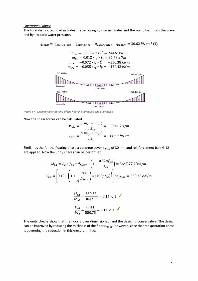
75

Operational phase The total distributed load includes the self-weight, internal water and the uplift load from the wave and hydrostatic water pressure.

𝑞𝑡𝑜𝑡𝑎𝑙 = 𝑞𝑠𝑒𝑙𝑓𝑤𝑒𝑖𝑔ℎ𝑡 − 𝑞𝑏𝑢𝑜𝑦𝑎𝑛𝑐𝑦 − 𝑞𝑤𝑎𝑣𝑒𝑢𝑝𝑙𝑖𝑓𝑡 + 𝑞𝑤𝑎𝑡𝑒𝑟 = 30.62 𝑘𝑁/𝑚2 (↓)

𝑚𝑣𝑥 = 0.032 ∗ 𝑞 ∗ 𝑙𝑥

2 = 244.61𝑘𝑁𝑚 𝑚𝑣𝑦 = 0.012 ∗ 𝑞 ∗ 𝑙𝑥

2 = 91.73 𝑘𝑁𝑚

𝑚𝑠𝑥 = −0.072 ∗ 𝑞 ∗ 𝑙𝑥2 = −550.38 𝑘𝑁𝑚

𝑚𝑠𝑦 = −0.055 ∗ 𝑞 ∗ 𝑙𝑥2 = −420.43 𝑘𝑁𝑚

Figure 87 - Moment distributions of the floor in x-direction and y-direction

Now the shear forces can be calculated.

𝑉𝑒𝑑𝑥=

2(𝑚𝑠𝑥 + 𝑚𝑣𝑥)

0.5𝑙𝑥= −77.41 𝑘𝑁/𝑚

𝑉𝑒𝑑𝑦=

2(𝑚𝑠𝑦 + 𝑚𝑣𝑦)

0.5𝑙𝑦= −66.47 𝑘𝑁/𝑚

Similar as the for the floating phase a concrete cover 𝑐𝑤𝑎𝑙𝑙 of 30 mm and reinforcement bars ∅ 12 are applied. Now the unity checks can be performed.

𝑀𝑟𝑑 = 𝐴𝑆 ∗ 𝑓𝑦𝑑 ∗ 𝑑𝑓𝑙𝑜𝑜𝑟 ∗ (1 −0.52𝑝𝑓𝑦𝑑

𝑓𝑐𝑑) = 3647.77 𝑘𝑁𝑚/𝑚

𝑉𝑟𝑑 = [0.12 ∗ (1 + √200

𝑑𝑓𝑙𝑜𝑜𝑟) ∗ (100𝑝𝑓𝑐𝑘)

13] 𝑏𝑑𝑓𝑙𝑜𝑜𝑟 = 550.75 𝑘𝑁/𝑚

𝑀𝑒𝑑

𝑀𝑟𝑑=

550.38

3647.77= 0.15 < 1

𝑉𝑒𝑑

𝑉𝑟𝑑=

77.41

550.75= 0.14 < 1

The unity checks show that the floor is over dimensioned, and the design is conservative. The design can be improved by reducing the thickness of the floor 𝑡𝑓𝑙𝑜𝑜𝑟. However, since the transportation phase

is governing the reduction in thickness is limited.

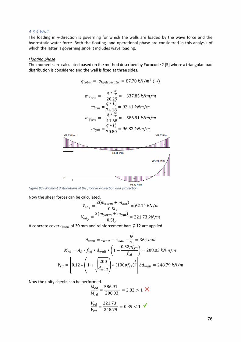
76

4.3.4 Walls The loading in y-direction is governing for which the walls are loaded by the wave force and the hydrostatic water force. Both the floating- and operational phase are considered in this analysis of which the latter is governing since it includes wave loading. Floating phase The moments are calculated based on the method described by Eurocode 2 [5] where a triangular load distribution is considered and the wall is fixed at three sides.

𝑞𝑡𝑜𝑡𝑎𝑙 = 𝑞ℎ𝑦𝑑𝑟𝑜𝑠𝑡𝑎𝑡𝑖𝑐 = 87.70 𝑘𝑁/𝑚2 (→)

𝑚𝑥𝑒𝑟𝑚= −

𝑞 ∗ 𝑙𝑦2

20.29= −337.85 𝑘𝑁𝑚/𝑚

𝑚𝑥𝑚 =𝑞 ∗ 𝑙𝑦

2

74.18= 92.41 𝑘𝑁𝑚/𝑚

𝑚𝑦𝑒𝑟𝑚= −

𝑞 ∗ 𝑙𝑦2

11.68= −586.91 𝑘𝑁𝑚/𝑚

𝑚𝑦𝑚 =𝑞 ∗ 𝑙𝑦

2

70.80= 96.82 𝑘𝑁𝑚/𝑚

Figure 88 - Moment distributions of the floor in x-direction and y-direction

Now the shear forces can be calculated.

𝑉𝑒𝑑𝑥=

2(𝑚𝑥𝑒𝑟𝑚 + 𝑚𝑥𝑚)

0.5𝑙𝑥= 62.14 𝑘𝑁/𝑚

𝑉𝑒𝑑𝑦=

2(𝑚𝑦𝑒𝑟𝑚 + 𝑚𝑦𝑚)

0.5𝑙𝑦= 221.73 𝑘𝑁/𝑚

A concrete cover 𝑐𝑤𝑎𝑙𝑙 of 30 mm and reinforcement bars ∅ 12 are applied.

𝑑𝑤𝑎𝑙𝑙 = 𝑡𝑤𝑎𝑙𝑙 − 𝑐𝑤𝑎𝑙𝑙 −∅

2 = 364 𝑚𝑚

𝑀𝑟𝑑 = 𝐴𝑆 ∗ 𝑓𝑦𝑑 ∗ 𝑑𝑤𝑎𝑙𝑙 ∗ (1 −0.52𝑝𝑓𝑦𝑑

𝑓𝑐𝑑) = 208.03 𝑘𝑁𝑚/𝑚

𝑉𝑟𝑑 = [0.12 ∗ (1 + √200

𝑑𝑤𝑎𝑙𝑙) ∗ (100𝑝𝑓𝑐𝑘)

13] 𝑏𝑑𝑤𝑎𝑙𝑙 = 248.79 𝑘𝑁/𝑚

Now the unity checks can be performed.

𝑀𝑒𝑑

𝑀𝑟𝑑=

586.91

208.03 = 2.82 > 1

𝑉𝑒𝑑

𝑉𝑟𝑑=

221.73

248.79= 0.89 < 1

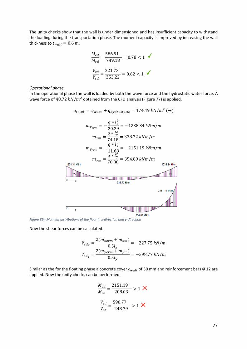
77

The unity checks show that the wall is under dimensioned and has insufficient capacity to withstand the loading during the transportation phase. The moment capacity is improved by increasing the wall thickness to 𝑡𝑤𝑎𝑙𝑙 = 0.6 𝑚.

𝑀𝑒𝑑

𝑀𝑟𝑑=

586.91

749.18 = 0.78 < 1

𝑉𝑒𝑑

𝑉𝑟𝑑=

221.73

353.22= 0.62 < 1

Operational phase In the operational phase the wall is loaded by both the wave force and the hydrostatic water force. A wave force of 48.72 𝑘𝑁/𝑚2 obtained from the CFD analysis (Figure 77) is applied.

𝑞𝑡𝑜𝑡𝑎𝑙 = 𝑞𝑤𝑎𝑣𝑒 + 𝑞ℎ𝑦𝑑𝑟𝑜𝑠𝑡𝑎𝑡𝑖𝑐 = 174.49 𝑘𝑁/𝑚2 (→)

𝑚𝑥𝑒𝑟𝑚= −

𝑞 ∗ 𝑙𝑦2

20.29= −1238.34 𝑘𝑁𝑚/𝑚

𝑚𝑥𝑚 =𝑞 ∗ 𝑙𝑦

2

74.18= 338.72 𝑘𝑁𝑚/𝑚

𝑚𝑦𝑒𝑟𝑚= −

𝑞 ∗ 𝑙𝑦2

11.68= −2151.19 𝑘𝑁𝑚/𝑚

𝑚𝑦𝑚 =𝑞 ∗ 𝑙𝑦

2

70.80= 354.89 𝑘𝑁𝑚/𝑚

Figure 89 - Moment distributions of the floor in x-direction and y-direction

Now the shear forces can be calculated.

𝑉𝑒𝑑𝑥=

2(𝑚𝑥𝑒𝑟𝑚 + 𝑚𝑥𝑚)

0.5𝑙𝑥= −227.75 𝑘𝑁/𝑚

𝑉𝑒𝑑𝑦=

2(𝑚𝑦𝑒𝑟𝑚 + 𝑚𝑦𝑚)

0.5𝑙𝑦= −598.77 𝑘𝑁/𝑚

Similar as the for the floating phase a concrete cover 𝑐𝑤𝑎𝑙𝑙 of 30 mm and reinforcement bars ∅ 12 are applied. Now the unity checks can be performed.

𝑀𝑒𝑑

𝑀𝑟𝑑=

2151.19

208.03 > 1

𝑉𝑒𝑑

𝑉𝑟𝑑=

598.77

248.79 > 1

78

The unity checks show that the wall is under dimensioned and has insufficient capacity to withstand the loading during operation. The wall capacity is improved by increasing the wall thickness to 𝑡𝑤𝑎𝑙𝑙 =1.2 𝑚.

𝑀𝑒𝑑

𝑀𝑟𝑑=

2151.19

6382.06 = 0.34 < 1

𝑉𝑒𝑑

𝑉𝑟𝑑=

598.77

646.29= 0.92 < 1

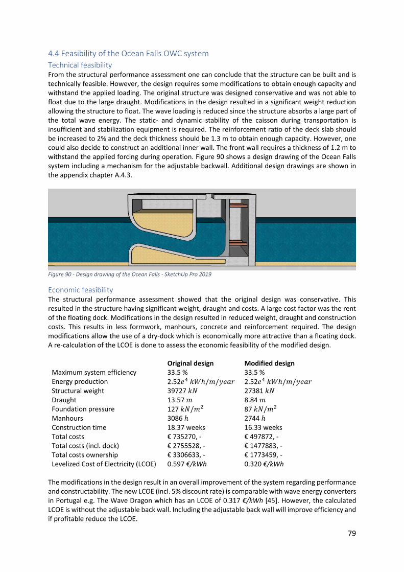
79

4.4 Feasibility of the Ocean Falls OWC system

Technical feasibility From the structural performance assessment one can conclude that the structure can be built and is technically feasible. However, the design requires some modifications to obtain enough capacity and withstand the applied loading. The original structure was designed conservative and was not able to float due to the large draught. Modifications in the design resulted in a significant weight reduction allowing the structure to float. The wave loading is reduced since the structure absorbs a large part of the total wave energy. The static- and dynamic stability of the caisson during transportation is insufficient and stabilization equipment is required. The reinforcement ratio of the deck slab should be increased to 2% and the deck thickness should be 1.3 m to obtain enough capacity. However, one could also decide to construct an additional inner wall. The front wall requires a thickness of 1.2 m to withstand the applied forcing during operation. Figure 90 shows a design drawing of the Ocean Falls system including a mechanism for the adjustable backwall. Additional design drawings are shown in the appendix chapter A.4.3.

Figure 90 - Design drawing of the Ocean Falls - SketchUp Pro 2019

Economic feasibility The structural performance assessment showed that the original design was conservative. This resulted in the structure having significant weight, draught and costs. A large cost factor was the rent of the floating dock. Modifications in the design resulted in reduced weight, draught and construction costs. This results in less formwork, manhours, concrete and reinforcement required. The design modifications allow the use of a dry-dock which is economically more attractive than a floating dock. A re-calculation of the LCOE is done to assess the economic feasibility of the modified design.

Original design Modified design Maximum system efficiency 33.5 % 33.5 % Energy production 2.52𝑒4 𝑘𝑊ℎ/𝑚/𝑦𝑒𝑎𝑟 2.52𝑒4 𝑘𝑊ℎ/𝑚/𝑦𝑒𝑎𝑟 Structural weight 39727 𝑘𝑁 27381 𝑘𝑁 Draught 13.57 𝑚 8.84 𝑚 Foundation pressure 127 𝑘𝑁/𝑚2 87 𝑘𝑁/𝑚2 Manhours 3086 ℎ 2744 ℎ Construction time 18.37 weeks 16.33 weeks Total costs € 735270, - € 497872, - Total costs (incl. dock) € 2755528, - € 1477883, - Total costs ownership € 3306633, - € 1773459, - Levelized Cost of Electricity (LCOE) 0.597 €/kWh 0.320 €/kWh

The modifications in the design result in an overall improvement of the system regarding performance and constructability. The new LCOE (incl. 5% discount rate) is comparable with wave energy converters in Portugal e.g. The Wave Dragon which has an LCOE of 0.317 €/kWh [45]. However, the calculated LCOE is without the adjustable back wall. Including the adjustable back wall will improve efficiency and if profitable reduce the LCOE.

80

5 Discussion and conclusions This chapter describes the results, conclusions and recommendations of the research.

5.1 Discussion First the results obtained from the parametric model, CFD model and the conceptual design are discussed. These discussion points should be carefully considered before going through the conclusions. For this research two models are applied: 1 - Parametric model (ANSYS AQWA and Python): Numerical frequency domain model which calculates the system performance in terms of power to the PTO and system efficiency. A Python script includes all differential equations required to model the Ocean Falls OWC system. Numerical diffraction software ANSYS AQWA is applied to calculate the hydrodynamic coefficients; added mass, radiation damping, diffraction and Froude-Krylov forcing in the frequency domain. 2 - CFD model (ANSYS Fluent): ANSYS Fluent software is applied for numerical modelling of the OWC system. The model provides insight in the system behavior, considers non-linear hydrodynamic effects and can simulate complex flow interaction. Further information about the model is provided in chapter A.3.7.1.

5.1.1 Parametric model For this research a parametric model is developed. The system behavior is characterized by hydrodynamic coefficients; added mass, radiation damping, diffraction and Froude-Krylov forcing. These coefficients are calculated with numerical diffraction software ANSYS AQWA. A python script converts the hydrodynamic coefficients into power output and system efficiency.

• The parametric model assumes that the water surface in the air chamber remains horizontal and behaves according to the rigid piston model. This assumption is valid for long waves but loses validity in case of short waves.

• The parametric model is linearized and assumes a linear relation between the air chamber pressure and the airflow through the turbine. However, the pressure-flow relation is quadratic and requires a non-linear analysis in the time domain. The linearized model assumes that ℎ𝑎𝑖𝑟 >> 𝑧 and is therefore unable to characterize a large pressure built up inside the air chamber. Therefore, the model underestimates the air chamber pressure for closed- and partly closed chamber conditions.

• The ANSYS AQWA model does not consider air chamber pressure and turbine damping. The model does not consider damping caused by friction, viscous losses, turbulence, vortex shedding and dissipation of energy from hydrodynamic effects and non-linear phenomena.

• The ANSYS AQWA model describes the diffraction pattern around the structure in 3D. The diffraction pattern from behind the structure results in additional wave reflection in front of the structure. This phenomenon affects the incoming waves and reduces the system efficiency. However, since the parametric model is 2D this effect is not included.

• In the parametric model there is no constraint for the maximum amplitude of the water surface elevation inside the air chamber. Therefore, the height of the air chamber could be insufficient during large oscillations of the internal water surface. The model does not account for this and calculates a higher efficiency whereas one should observe a reduced efficiency.

81

• The overall efficiency of the conversion from wave to wire consists of the efficiency of the OWC system, the efficiency of the turbine and the efficiency of the generator. In this research only the efficiency of the OWC system is considered.

5.1.2 CFD model For this research a Computational Fluid Dynamics model (CFD) is set-up in ANSYS Fluent. This model allows for large wave- and body motions and can deal with complexities in geometry e.g. curves and sharp edges. The model accounts for non-linear hydrodynamic effects and can describe a non-linear pressure-flow relation which is more realistic. The CFD model has no issues dealing with resonating water surfaces which is essential for the performance of the Ocean Falls OWC system. The CFD model is applied to assess the validity of the linearized parametric model.

• The CFD model showed that the rigid piston approach loses validity for short period waves (𝑇 < 6.5 𝑠). In that case the water surface in the air chamber does not remain horizontally flat.

• The CFD model can describe the non-linear relation between the air chamber pressure and the airflow through the turbine. This results in an improved estimate of the air chamber pressure and air compressibility.

• The CFD model can quantify friction, viscous losses, turbulence, vortex shedding and dissipation of energy from other non-linear hydrodynamic effects. The model does also account for the effect of variable air pressure in the air chamber.

• The CFD model is 2D and considers single-directional regular waves and does not account for irregular waves or multiple wave directions.

• The CFD model does not include marine growth. However, marine growth affects the system mass, wall friction, natural frequency and system performance.

• The wave boundary in the CFD model is reflective which results in additional wave reflection. This effect is minimized by applying a wave tank length of approximately 3 times the maximum wave length. The results of a wave reflection analysis show a difference in maximum internal water surface elevation amplitude of 12%. This difference is likely due to wave reflection from the reflective wave boundary.

• In the CFD model the air chamber pressure is measured in a single point close to the outlet on top of the air chamber. Measuring the pressure in multiple points would improve the pressure estimate.

82

5.1.3 Conceptual design For this research a conceptual design of the Ocean Falls is made to assess the technical feasibility. The structural performance of the design is assessed based on design checks. The objective is to ensure that the structure fulfils both functional- and structural requirements. The design should be considered as a preliminary design of the Ocean Falls structure.

• A concept case is applied to decide on a design by including constructability aspects. However, to more accurately assess the technical- and economic feasibility of the structure the construction method for the chosen design should be optimized.

• Deciding on a geometry out of all designs is done by applying the same construction method. However, finding the most cost-effective construction method for a specific design is not done. This could possibly result in different design becoming more attractive in terms of constructability and cost effectiveness.

• The structural designs have not been modified prior to deciding on a design. Design modifications are only done for the conceptual design of the Ocean Falls. This is due to the iterative process being an integral part of this research.

• For the structural performance assessment of the Ocean Falls a selection of design checks are done. One should keep in mind that the objective of the conceptual design is to obtain a first estimate of the technical feasibility of the Ocean Falls. However, additional checks are required to guarantee the structural performance.

• The construction costs include only the direct cost which include materials, equipment, manhours, construction and the (dry- or floating) dock costs. The costs of civil works are limited to the concrete, reinforcement, formwork and labour. However, the installation costs, indirect costs and costs for local modifications in reinforcement and formwork are not included.

• The formwork, reinforcement and dock costs are a substantial part of the total construction costs. Because the cost calculation is done for only a single unit; the effect of repetition is not considered. Repetition is expected to reduce the total project costs since large savings can be obtained through repetition of e.g. formwork and construction methods.

• For the conceptual design it is assumed that the elements in the structure are simple, straight and plane. Special shapes e.g. curved corners which require local modifications in formwork are not considered.

• The dynamic loads from pressure- and oscillation of the internal water surface in the air chamber are not considered in the conceptual design. The oscillation of the rigid body in the connection tube is also not considered. The internal water surface oscillation affects the point of gravity and is likely to influence the rotational stability of the structure during operation.

83

5.2 Conclusions This section elaborates on the conclusions of the research which provide an answer to the main research question: ‘’How to assess the technical feasibility of the Ocean Falls OWC system based on performance and structural requirements?’’

The research questions defined in the beginning of the report are introduced again. ‘’What is the effect of the geometry; width of the air chamber, height of the connection tube and length of the connection tube on the system performance?’’ System performance represents the system efficiency which is defined as the power available to the power take-off system (PTO) divided by the available wave energy flux. The system behavior depends on the structural geometry for which a total of 13 designs are developed each with a different geometry. For each design the effect on the system performance and first system natural frequency is investigated aiming to find a preferred geometry and design. The parameters that define the geometry of the structure are the height of the connection tube 𝐴, width of the air chamber 𝐵 and the length of the connection tube 𝐿. Maximum system performance is obtained once the device operates in resonance conditions. In that case the system natural period matches the (average) incoming wave period. Changing the parameter 𝐴, 𝐵 or 𝐿 results in a change of the system natural frequency. The characteristic of the Ocean Falls system is the ability to change the air chamber width 𝐵 with an adjustable back wall. Therefore, the width 𝐵 can be adjusted such that the system natural period and the (average) wave period match causing the device to operate in resonance conditions. In the parametric model the hydrodynamic coefficients are obtained from numerical diffraction software ANSYS AQWA and provide insight in the system behaviour. In the numerical frequency domain model these hydrodynamic coefficients are converted into a value of system performance by a Python script. All designs are compared with respect to a base case geometry; 𝐴 = 5.32 m, 𝐵 = 5.37 m, 𝐿 = 13.05 m. In theory and with respect to the base case a value of 𝐴 > 5.32 m results in a reduced performance and a value of 𝐴 < 5.32 m improves performance. In case 𝐵 > 5.37 m the performance improves while 𝐵 < 5.37 m reduces performance. Likewise, 𝐿 > 13.05 m improves performance and 𝐿 < 13.05 m reduces performance. However, the performance depends on the wave statistics which are site specific. Based on these results one can conclude that theoretically a design with a small 𝐴, a large 𝐵 or a large 𝐿 is preferred. However, these parameters are related and the combination of 𝐴, 𝐵 and 𝐿 should be considered. 𝐴: The height of the connection tube determines the volume of water and wave energy that can be absorbed by the system. Therefore, the height of the tube should be large enough to capture and absorb the available wave energy. In case the wave height > 𝐴 the device is unable to capture all available wave energy and becomes inefficient. In case 𝐴 is small the wave forcing on the front wall is high since less water is absorbed by the system. 𝐵: The width of the air chamber should be based on the operational wave period and determines the resonance characteristics of the system. However, the CFD model showed that the turbulence intensity is highly influenced by the 𝐵/𝐴 ratio. To minimize hydraulic losses caused by turbulence and other hydrodynamic effects; the 𝐵/𝐴 ratio should stay in-between 0.75 – 2.5. Therefore, the range of 𝐵 is limited and one should tune the average frequency of the system with the length of the connection tube 𝐿.

84

‘’What is the effect of irregular waves on the system performance?’’ The system efficiency is calculated with the parametric model including an optimal turbine damping parameter 𝐾𝑡𝑢𝑟𝑏𝑖𝑛𝑒. For the designs with variable 𝐴 the system efficiency for regular waves ranges from 55% to 90% whereas for irregular waves the efficiency ranges from 25.5% to 33%. Likewise, for the designs with variable 𝐵 the system efficiency for regular waves ranges from 45% to 91% whereas the efficiency for irregular waves ranges from 22% to 36%. Finally, for the designs with variable 𝐿 the system efficiency for regular waves ranges from 61% to 90% whereas for irregular waves the efficiency ranges from 27% to 33.5%. One can conclude that irregular waves have a significant impact on the system efficiency. For irregular waves the system efficiency is highly sensitive to the peakedness factor 𝛾 which depends on the irregularity of the sea-state at the project location. Therefore, this parameter should be carefully considered while deciding on a project location. The range of efficiencies for either regular- or irregular waves is the largest for the parameter 𝐵. Therefore, one can conclude that the width of the air chamber 𝐵 is the decisive parameter for the overall performance of the system. ‘’What is the extent of validity of a linearized parametric model?’’ A CFD model of the Ocean Falls is applied to assess the validity of the linearized parametric model. However, first the accuracy of the CFD model is assessed by comparing the CFD model with model scale experiments of the Ocean Falls. The CFD model shows a similar system response and trends as obtained from model scale experiments. The ratio of the water surface elevation amplitude over incoming wave amplitude of both models is also in the same order of magnitude. Therefore, the CFD model is applied to assess the validity of the linearized parametric model. The CFD model showed that the original design has insufficient capacity to include the total volume of water during operation. Therefore, the height of the air chamber should be extended to increase the total system capacity. The internal water surface elevation and air chamber pressure of both the parametric- and CFD model are compared for open-, closed- and partly-closed chamber conditions. For open chamber conditions where air chamber pressure and turbine damping are excluded the difference in maximum amplitude of the internal water surface is 7%. The air chamber pressure obtained from both the numerical- and CFD model are the same and the difference in period is 10%. For a range of wave periods the parametric model underestimates the resonance period and the internal water surface elevation. This is likely due to an overestimation of the radiation damping and an underestimation the system mass.

For closed chamber conditions the effect of air chamber pressure is included. The parametric model underestimates the air chamber pressure since the model assumes that ℎ𝑎𝑖𝑟 >> 𝑧. However, in the non-linear CFD model this assumption is not valid resulting in higher pressures. For partly closed chamber conditions the effects of air chamber pressure and turbine damping are included. The results show that the parametric model underestimates both the internal water surface elevation amplitude and the air chamber pressure. This is likely due to the parametric model overestimating the turbine damping. Based on the comparison of both models it can be concluded that the parametric model requires an improved estimate of the system mass. The parametric model should also include a constraint for the maximum amplitude of the water surface elevation in the air chamber. One can conclude that assuming a linear pressure-flow relation in the parametric model is incorrect and a non-linear analysis in the time domain is required. The assumption ℎ𝑎𝑖𝑟 >> 𝑧 would then become invalid, the pressure-flow relation becomes quadratic and the pressure distribution becomes cubic which is more realistic. On average the parametric model differs 15-20 % from the CFD model.

85

‘’How to obtain an “optimal” design based on both system performance and constructability aspects?’’ A decision is made based on three criteria: system performance, constructability and cost effectiveness.

System performance An irregular wave spectrum at a project location in Portugal has an available wave energy flux of 10.1 𝑘𝑊/𝑚. At this location the power production of each design is calculated. For the designs with variable 𝐴 the power production ranges from 2.08 𝑘𝑊/𝑚 to 2.87 𝑘𝑊/𝑚. The power production of the designs with variable 𝐵 ranges from 1.63 𝑘𝑊/𝑚 to 3.30 𝑘𝑊/𝑚. Finally, the power production of the designs with variable 𝐿 ranges from 2.02 𝑘𝑊/𝑚 to 2.93 𝑘𝑊/𝑚. The range of power production is the largest for the designs with variable 𝐵. Therefore, based on system performance one should opt for a design with a large 𝐵.

The device is most efficient while operating in near-resonance conditions where the system natural period matches the (average) incoming wave period. In case one opts for a design with a large 𝐵 the system has more mass resulting in a longer natural period. However, in case the wave spectrum is dominated by short wave periods this design is inefficient and certainly not preferred. The Ocean Falls system can change its natural period by adjusting the position of the back wall resulting in a different air chamber width 𝐵. Therefore, this system can remain efficient independent of the different wave periods in the wave spectrum. An analysis done with a changing air chamber width 𝐵 resulted in a power production of 3.71 𝑘𝑊/𝑚 at the chosen project location which is equivalent to an efficiency of 37%. One can conclude that the system efficiency is improved with 12% respectively to an OWC system with a fixed back wall position. Constructability By applying constructability aspects the required manhours, concrete, weight, draught and foundation pressure of the different designs are calculated. A design with a large 𝐵 might produce more energy but requires additional concrete, space and reinforcement. Likewise, a design with a small 𝐴 might be more attractive in terms of system performance but less attractive in terms of constructability e.g. concrete, reinforcement and manhours. These relations result in different designs becoming attractive than based on solely system performance. Cost effectiveness To eventually decide on a design, the costs of each design are calculated and compared with the total energy production over the service lifetime. For comparison the Levelized Cost of Electricity (LCOE) is calculated for each design. Those designs having a low LCOE are to be preferred. The LCOE of the preferred design equals 0.597 €/kWh which is comparable to conventional WEC systems at the project location. “How to make a conceptual design of the Ocean Falls which fulfills both structural and performance requirements?” The structural performance of the Ocean Falls is assessed by applying several design checks to ensure that the structure does not fail, collapse or is seriously damaged due to the applied loading. One can conclude that the original structure was designed conservative which resulted in a significant weight and draught. Because the water depth at the project location does not allow a draught > 10.5 m floating of the caissons was impossible. Modifications in the design resulted in a more material-efficient and less conservative structure. The structure is designed for a design wave height 𝐻 =4.55 𝑚 and 𝑇 = 9 𝑠 which results in a large wave pressure on the structure. However, a CFD analysis showed that the wave pressure is reduced because the system absorbs a part of the total wave energy.

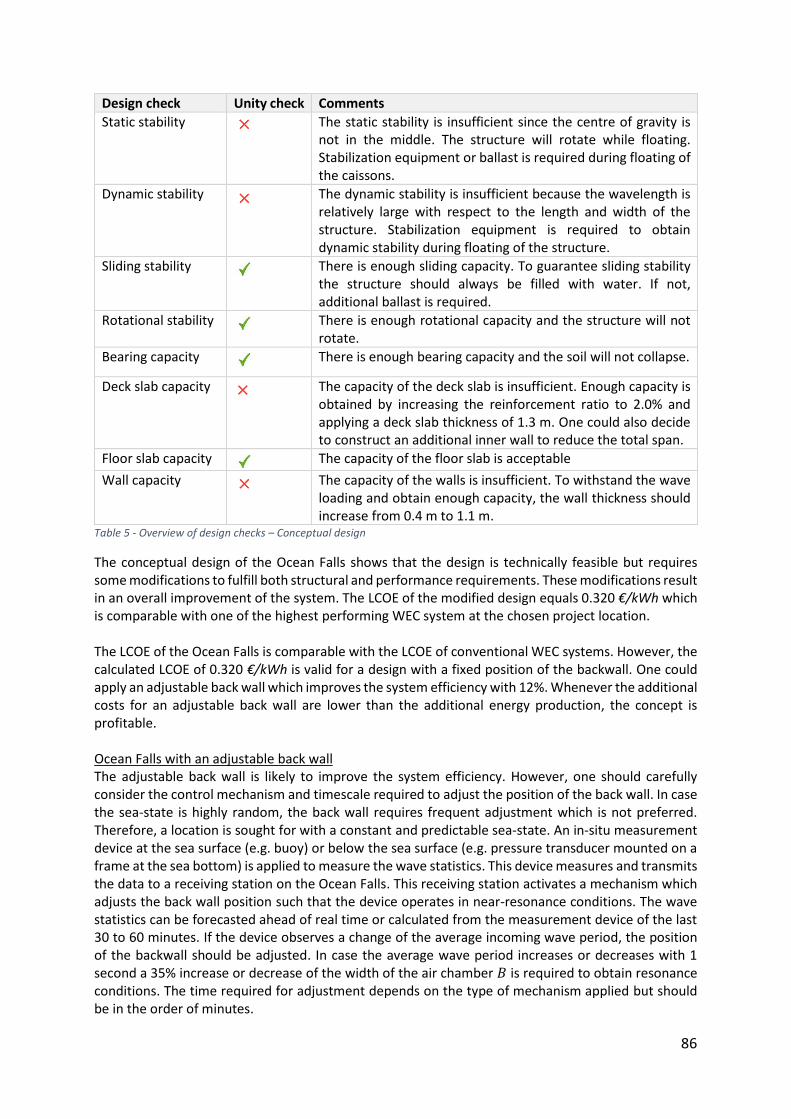
86

Design check Unity check Comments

Static stability

The static stability is insufficient since the centre of gravity is not in the middle. The structure will rotate while floating. Stabilization equipment or ballast is required during floating of the caissons.

Dynamic stability The dynamic stability is insufficient because the wavelength is relatively large with respect to the length and width of the structure. Stabilization equipment is required to obtain dynamic stability during floating of the structure.

Sliding stability There is enough sliding capacity. To guarantee sliding stability the structure should always be filled with water. If not, additional ballast is required.

Rotational stability There is enough rotational capacity and the structure will not rotate.

Bearing capacity There is enough bearing capacity and the soil will not collapse.

Deck slab capacity The capacity of the deck slab is insufficient. Enough capacity is obtained by increasing the reinforcement ratio to 2.0% and applying a deck slab thickness of 1.3 m. One could also decide to construct an additional inner wall to reduce the total span.

Floor slab capacity The capacity of the floor slab is acceptable

Wall capacity The capacity of the walls is insufficient. To withstand the wave loading and obtain enough capacity, the wall thickness should increase from 0.4 m to 1.1 m.

Table 5 - Overview of design checks – Conceptual design

The conceptual design of the Ocean Falls shows that the design is technically feasible but requires some modifications to fulfill both structural and performance requirements. These modifications result in an overall improvement of the system. The LCOE of the modified design equals 0.320 €/kWh which is comparable with one of the highest performing WEC system at the chosen project location. The LCOE of the Ocean Falls is comparable with the LCOE of conventional WEC systems. However, the calculated LCOE of 0.320 €/kWh is valid for a design with a fixed position of the backwall. One could apply an adjustable back wall which improves the system efficiency with 12%. Whenever the additional costs for an adjustable back wall are lower than the additional energy production, the concept is profitable. Ocean Falls with an adjustable back wall The adjustable back wall is likely to improve the system efficiency. However, one should carefully consider the control mechanism and timescale required to adjust the position of the back wall. In case the sea-state is highly random, the back wall requires frequent adjustment which is not preferred. Therefore, a location is sought for with a constant and predictable sea-state. An in-situ measurement device at the sea surface (e.g. buoy) or below the sea surface (e.g. pressure transducer mounted on a frame at the sea bottom) is applied to measure the wave statistics. This device measures and transmits the data to a receiving station on the Ocean Falls. This receiving station activates a mechanism which adjusts the back wall position such that the device operates in near-resonance conditions. The wave statistics can be forecasted ahead of real time or calculated from the measurement device of the last 30 to 60 minutes. If the device observes a change of the average incoming wave period, the position of the backwall should be adjusted. In case the average wave period increases or decreases with 1 second a 35% increase or decrease of the width of the air chamber 𝐵 is required to obtain resonance conditions. The time required for adjustment depends on the type of mechanism applied but should be in the order of minutes.

87

Ocean Falls with a fixed back wall position In case one decides not to apply an adjustable back wall the Ocean Falls OWC system still shows high potential. In that case it is advised to choose a location with a constant sea-state and less seasonal variation. The system should then be dimensioned such that the system natural period matches the average wave period at this location. Since the system mass determines the system natural frequency and most of the mass depends on the dimensions of the connection tube; 𝐴 and 𝐿 are decisive. One could then improve the system efficiency by applying different turbines for low and long period waves respectively. One can conclude that the Ocean Falls OWC system has a high potential either with or without the adjustable back wall. However, to compete with conventional OWC systems one can lower the LCOE by considering the following aspects:

1) Suitable location: One should choose a location with a constant wave climate and a dominant average wave period of 8.5-9.5 s. As a result, the device will operate in near-resonance conditions and produce maximum power.

2) Include the adjustable back wall: Including this feature has proven to increase the system efficiency with 12%.

3) Concentrated wave energy flux: One could improve the absorption of wave energy by the installation of guiding walls towards the inlet of the structure.

4) Integrated OWC system: By integrating the Ocean Falls OWC system into e.g. an existing breakwater one could reduce CAPEX and OPEX costs.

5) Location dependent geometry: One could dimension the structure such that the system natural period matches the (average) incoming wave period. As a result, the device will operate in near-resonance conditions and produce maximum power.

6) Multiple units: Large scale production reduces the CAPEX per device through learning, innovation and repetition.

7) Distance to shore: The mean wave power, mooring costs, grid costs and transit cost depend on the distance to shore. To minimize these costs the device should be built close to the shore.

5.3 Recommendations for further research This section gives an overview of the recommendations and proposals for further research projects.

• The effect of wave diffraction behind the structure is likely to induce additional wave reflection in front of the structure which affects the system efficiency. One could exclude this effect by extending the width of the structure as shown in Figure A.3.4. To obtain insight in the effect of additional wave reflection one should develop a 3D CFD model.

• The ANSYS AQWA model of the Ocean Falls considers open chamber conditions and does not account for air chamber pressure, air compressibility and turbine damping. To include these effects, one could improve the model or apply different software which is able to include these effects.

• For a range of wave periods the results obtained from the parametric model are compared with the results from the CFD model for open chamber conditions. One should perform a similar analysis including the effects of air chamber pressure and turbine damping.

• The total energy production at the project location is calculated for a fixed range of wave heights and wave periods. However, at the project location there are several waves outside of this range which are not included. Extending the range of wave frequencies in the parametric model will improve the total energy production.

88

• A CFD model including marine growth showed that marine growth affects the system performance and should not be neglected. The marine growth is not included in the CFD model applied for this research. However, one should consider the influence of marine growth in the final design of the Ocean Falls.

• The ANSYS AQWA model of the Ocean Falls should be modified to ensure that the height of the system inlet is constant for different lengths of the connection tube.

• The parametric model should include a constraint for the maximum amplitude of the water surface elevation inside the air chamber.

• Further research is required to investigate potential risks of the system regarding e.g. airtightness of the air chamber, marine growth and the adjustable back wall.

• Further research is required to investigate the effect of tidal variation on the system efficiency. In case tidal variation is significant the tube could become only partly submerged which reduces system efficiency. A solution could be to make a floating OWC device.

• Further research is required to investigate the effect of multi-directional waves on the system efficiency.

• Including an adjustable back wall allows the device to operate more frequently in resonance conditions which improves the system efficiency. However, constructability, design and the control mechanism of the adjustable back wall should be investigated to assess the feasibility.

89

6 Bibliography

[1] W. Sheng, Wave energy conversion and hydrodynamic modelling technologies: A review, Elsevier Ltd, 2019, From: https://www.sciencedirect.com/science/article/pii/S1364032119302424

[2] Baez Rivero, Inés. Investigation of the robustness of an Oscillating Water Column breakwater under extreme wave conditions, Msc. Thesis, TU Delft, Delft, 2018. From: https://repository.tudelft.nl

[3] N. Khan, A. Kalair, N. Abas, A. Haider, Review of ocean tidal, wave and thermal energy technologies, Elsevier Ltd, 2017. From: https://ideas.repec.org/a/eee/rensus/v72y2017icp590-604.html

[4] A. Falcao, Modelling of Wave Energy Conversion, IST University of Lisboa, Portugal, 2014. From: https://fenix.tecnico.ulisboa.pt/ 3779580629428

[5] European Committee, Eurocode 2 - Design of concrete structures, Brussels, 2019. From: http://pr01.silverhost.cl/part_4_eurocode_2_design_of_concrete_structures.pdf

[6] A. Falcao and J.C.C. Henriques, Oscillating-water-column wave energy converters and air turbines: A review, IST University of Lisboa, Portugal, 2016. From: https://www.researchgate.net/publication/281307478

[7] M.I. Kelkitli, Analysis of the Ocean Falls Wave Energy Converter in Regular Waves. Msc. Thesis, TU Delft, Delft, 2018. From: https://repository.tudelft.nl

[8] A. Falcao, Renewable Energy, IST University of Lisboa, Portugal, 2015. From: https://www.researchgate.net/publication/281307475

[9] J.K. Vrijling, W.F. Molenaar, Manual Hydraulic Structures, Civil Engineering and Geosciences, TU Delft, Delft, 2016. From: https://repository.tudelft.nl

[10] R.P.F. Gomes, J.C.C. Henriques, L.M.C. Gato, and A. Falcao, Hydrodynamic optimization of an axisymmetric floating oscillating water column for wave energy conversion. Agris Journal Article, 2012. From: http://agris.fao.org

[11] S.L. Dixon, Fluid Mechanics, Thermodynamics of Turbomachinery 4th Edition, University of Liverpool, England, 1998. From: http://160592857366.free.fr/joe/ebooks/Mechanical%20Engineering%20Books%20Collection

[12] K. Hasselmann, Measurements of wind- wave growth and swell decay during the joint North Sea wave project (JONSWAP), Germany, 1973. From: https://repository.tudelft.nl

[13] ANSYS Inc. ANSYS AQWA Theory Manual. USA, 2017. From: https://support.ansys.com

[14] Y. Washio, Journal of the Marine Engineering Society in Japan, Japan, 2018 https://www.jstage.jst.go.jp/article/jime1966

[15] URS, Wave power feasibility study report, San-Francisco, 2009. From: https://sfenvironment.org/sites/default/files/fliers/files/sfe_en_wave_feasibilty_report.pdf

[16] J. Falnes, Ocean Waves and Oscillating Systems, Cambridge University Press, Cambridge, 2002. From: https://www.cambridge.org/core/books/ocean-waves-and-oscillating-systems

[17] A. Falcao and J. C.C. Henriques. Model-prototype similarity of oscillating-water-column wave energy converters. International Journal of Marine Energy, Elsevier Ltd, 2014. From: https://www.sciencedirect.com/science/article/pii/S2214166914000058

[18] E. Ten Oever, Market potential, Delta Marine Consultants (DMC), Gouda, 2009. From: https://www.researchgate.net/profile/Erik_Ten_Oever

90

[19] B. Stappenbelt and P. Cooper. Mechanical model of a floating oscillating water column wave energy conversion device. University of Wollongong, Australia, 2010. From: https://ro.uow.edu.au

[20] R.P.F. Gomes, J.C.C.Henriques, L.M.C.Gato, A. Falcao. Wave power extraction of a heaving floating oscillating water column in a wave channel. IST University of Lisboa, Portugal, 2015. From: https://www.sciencedirect.com/science/article/pii/S0960148116307133

[21] V. Sundar, T. Moan, J. Hals. Conceptual design of OWC wave energy converters combined with breakwater structures, Offshore and artic engineering Shanghai, China, 2010. From: https://www.researchgate.net/publication/287843022

[22] J. Henriques, J. Portillo, L. Gato, R. Gomes, D. Ferreira, A. Falcao, Design of oscillating water column wave energy converters with an application of self-powered sensor buoys, IST University of Lisboa, Portugal, 2016. From: https://www.researchgate.net/publication/306313216

[23] G.J. Dalton, R. Alcorn, T. Lewis, Case study feasibility analysis of the Pelamis wave energy convertor in Ireland. University College Cork, Ireland, 2010. From: http://dx.doi.org/10.1016/j.renene.2009.07.003.

[24] M. Voorendt, W.F. Molenaar, K.G. Bezuyen, Lecture notes Caissons, TU Delft, Delft, 2011. From: https://repository.tudelft.nl

[25] O. Malmo, Wave power absoption by oscillating water column in a channel, Journal of fluid dynamics, University of Trondheim Norway, Norway, 1985. From: https://www.cambridge.org/core/journals/journal-of-fluid-mechanics

[26] J. Cruz, Ocean wave energy: current state and future perspectives, Garrad Hassan and Partners Ltd, Bristol, 2008. From: https://www.researchgate.net/publication/291994394

[27] Smartsheet Inc , Demistifying the 5 stages of project management, Washington, 2018. From: https://www.smartsheet.com

[28] M.I.T, OpenCoarseWare, Massachusetts Institute of Technology, Massachusetts, 2009. From: https://ocw.mit.edu/courses

[29] G. Moretti, G. Pietro, Resonant wave energy harvester based on dielectric elastomer generator, TeCIP Institute, Scuola Superiore Sant’Anna, 2018. From: https://iopscience.iop.org/article/10.1088

[30] ASME – Digital collection , Uncertainty in peakedness factor estimation by JONSWAP spectral fitting from measurements, USA, 2018. From: http://proceedings.asmedigitalcollection.asme.org/proceeding.aspx?articleid=1786406

[31] A. Falcao and R.J.A. Rodrigues, model prototype similarity of oscillating- water column wave energy converters. International Journal of Marine Energy, IST University of Lisboa, Portugal, 2014. From: https://www.researchgate.net/publication/291994334

[32] LMC Gato and A. Falcao. On the theory of the Wells turbine. Journal of engineering for gas turbines and power, Portugal, 1984. From: https://www.researchgate.net/publication/245352078

[33] A. Falcao, Wave energy utilization: A review of the technologies, Elsevier Ltd. 2010. From: https://www.sciencedirect.com/science/article/pii/S1364032109002652

[34] A. Falcao, Air turbine optimization for a bottom-standing OWC wave energy converter, Journal of Ocean Engineering and Marine Energy, IST University of Lisboa, Portugal, 2016. From: https://www.researchgate.net/publication/295830323

[35] S. Ribeiro e Silva, Hydrodynamic optimization of the UGEN: Wave Energy Converter with U-shaped interior oscillating waver column, Conference paper, IST University of Lisboa, Portugal, 2015. From: https://www.researchgate.net/publication/282150443

[36] J. Tuin, Optimal construction and transportation method for gravity-based foundations for offshore windfarms on commercial scale, TU Delft, Delft, 2018. From: https://repository.tudelft.nl

91

[37] A. van der Horst, Lecture notes construction technology of Civil Engineering Projects, TU Delft, Delft, 2018. From: https://repository.tudelft.nl

[38] E. Ten Oever, Resonance Wave Energy Converter, Delta Marine Consultants (DMC), Gouda, 2008.

[39] M.Z. Voorendt, Hydraulic Structures Caissons, Civil engineering and Geosciences, TU Delft, Delft, 2016. From: https://repository.tudelft.nl [40] DNV-GL, rules and standards, 2018. From: https://www.dnvgl.com [41] C. Soares, Renewable energies offshore, Centre of Marine Technology and Ocean Engineering (CENTEC), IST University of Lisboa, Portugal, 2015. From: https://books.google.nl/books?id=nNCYCgAAQBAJ [42] H. Bingham, Hydrodynamic analysis of oscillating water column wave energy devices, Journal of Ocean Engineering and Marine Energy, Technical University of Denmark, Denmark, 2015. From: https://www.researchgate.net/publication/281146253 [43] The Grid, The Levelized Cost of Electricity: Definition and Example, 2018. From https://thegrid.rexel.com/en-us/knowledge/energy-efficiency [44] A. Falcão, J.C.C. Henriques, L.M.C. Gato, and R.P.F. Gomes. Air turbine choice and optimization for floating oscillating-water-column wave energy converter. Elsevier Ltd, 2018. From: https://www.sciencedirect.com/science/article/pii/S0029801813003892 [45] L. Castro-Santos, D. Silva, A. Rute Bento, N. Salvação, C. Guedes Soares, Economic feasibility of wave energy farms in Portugal, IST University of Lisboa, Portugal, 2018. From: https://www.mdpi.com/1996-1073/11/11/3149 [46] NOAA (National Oceanic and Atmospheric Administration), bathymetric data viewer, 2018, From: https://maps.ngdc.noaa.gov [47] G.J. Schiereck, H.J. Verhagen, Introduction to bed, bank and shore protection, Civil Engineering and Geosciences, TU Delft, Delft, 2016. From: https://repository.tudelft.nl

[48] ANSYS Inc. ANSYS FLUENT users guide, USA, 2009. From: http://www.afs.enea.it/project/neptunius/docs/fluent

[49] J.M.J. Journée, W.W. Massie, and R.H.M. Huijsmans, Offshore Hydromechanics, TU Delft, Delft TU Delft Press, 2000. From: https://ocw.tudelft.nl/wp-content/uploads/OffshoreHydromechanics_Journee_Massie.pdf [50] J. Kruit, Technology Readiness Levels (TRL), Innovencio,2017. From: https://innovencio.nl/technology-readiness-levels/ [51] The Physics Classroom, Behavior of waves, 2019, From: https://www.physicsclassroom.com/class/waves/Lesson-3/Reflection,-Refraction,-and-Diffraction [52] TPUB, Coastal engineering manual – Linear wave theory, 2002. From: http://coastalengineeringmanual.tpub.com/Part-II-Chap1/Part-II-Chap10011.htm [53] P. Boccotti, Comparison between a U-OWC and a conventional OWC , Ocean Engineering, 2007, From: https://www.researchgate.net/publication/245196099 [54] J. Henriques, W. Sheng, A. Falcão, L.M.C. Gato , A comparison of Biradial and Wells air turbines on the Mutriku Breakwater OWC Wave Power Plant , International Conference on Ocean, Offshore and Artic Engineering, 2017, From: https://www.researchgate.net/publication/318471691 [55] S. Johnson, S. Kumar, T. Thachuparumbil, V. Joseph John , Design and analysis of 3D blades for Wells turbine, Saintgits College of Engineering, Department of Mechanical Engineering, 2015, From: http://www.ijirst.org/articles/IJIRSTV1I11064.pdf [56] D. Waves, Economic aspects of Ocean energy, Joint Research Centre, Delft, 2018, From: JRC [57] A. Kamath, H. Bihs, A. Arntsen, Comparison of 2D and 3D simulations of an OWC device in different configurations, Coastal engineering 2014, From: https://journals.tdl.org/icce/index.php/icce/article/viewFile/7785/pdf_892

92

[58] V. Evans, Oscillating Water Column wave energy converters , IMA Journal of applied mathematics, 1978, From: https://www.researchgate.net/publication/243083403_The_Oscillating_Water_Column_Wave-energy_Device [59] J.N.A Sarmento, Wave flume experiments on two-dimensional oscillating water column wave energy devices , Experiments in fluids, 1992, From: https://link.springer.com/article/10.1007/BF00187307 [60] Y. Zhang, Air-water two phase flow modelling of hydrodynamic performance of an oscillating water column device, Renewable energy, 2012, From: https://www.researchgate.net/publication/251627323 [61] J.G. Gonzalez, Numerical modelling in turbines for OWC systems: Application to a radial impulse, OMAE, Shanghai, 2010, From: https://www.researchgate.net/publication/256473709 [62] E. Medina-Lopez, Maria Clavero, simulation of a simple OWC problem for turbine performance, International Journal of Marine Energy 20, University of Granada, Spain, 2017, From: https://www.researchgate.net/publication/321167204 [63] W. Sheng, F. Thiebaut, M. Babuchon, J. Brooks, A. Lewis, R. Alcorn, Investigation to air compressibility of oscillating water column wave energy converters, International conference on marine offshore mechanics and artic engineering, Nantes, France, 2013. From: http://proceedings.asmedigitalcollection.asme.org/proceeding.aspx?articleid=1786694 [64] L. Holthuijsen. Waves in oceanic and coastal waters. Cambridge university press, 2010. Fromhttp://www.sisal.unam.mx/labeco/LAB_ECOLOGIA/OF_files/82571738-Waves-in-Oceanic-and-Coastal-Waters.pdf

[65] J.M. van der Jagt, Wave Energy Converters, A methodology for assessing power performance, applied to a quasi-rigid submerged pressure differential device, Msc. Thesis, TU Delft, Delft, 2018. From: https://repository.tudelft.nl

[66] I. Lopez, G. Iglesias, Efficiency of OWC wave energy converters: A virtual laboratory, Applied Ocean Research, University of Sntiago de Compostela, Spain, 2012. From: https://www.sciencedirect.com/science/article/pii/S0141118713000886

[67] R.G. Dean, R.A. Dalrymple, Water Wave Mechanics for Engineers and Scientists, World Scientific Publishing, Singapore, 1991. From: https://books.google.nl/books?hl=nl&lr=&id=1SM8DQAAQBAJ&oi=fnd&pg=PR7&ots=H6J5-C49WB&sig=jDkwT-Fi6WiReAJTDM8NrIXwsZ4&redir_esc=y#v=onepage&q&f=false

[68] S.P. Neil, M. Reza Hashemi, Fundamentals of Ocean Renewable Energy – generating electricity from the sea, E-Business solutions, 2018. From: https://www.sciencedirect.com/book/9780128104484/fundamentals-of-ocean-renewable-energy

[69] Department of Business, Feasibility of developing wave power as a renewable energy resource for Hawaii, Hawaii, 2002. From: https://energy.hawaii.gov/wp-content/uploads/2011/10/Feasibility-of-Developing-Wave-Power-as-a-Renewable-Energy-Resource-for-Hawaii.pdf

[70] M. Lino, T. Miyazaki, H. Segawa, M. Lida, Effect of inclination on oscillation characteristics of an oscillating water column wave energy converter, Ocean Engineering vol. 116, 2016. From: https://www.sciencedirect.com/science/article/pii/S0029801816001219

[71] C.V.C. Weiss, R. Guanche, B. Ondiviela, O.F. Castellanos, J. Juanes, Energy conversion and management, Environmental Hydraulic Institute, University of Cantabria, Spain, 2018. From: https://reader.elsevier.com/reader/sd/pii/S0196890418310628?token=B0FBA78C95C986560C0F3021E30D2A058638C700C598F5CCBA8D57226001A4D462C8407534A9BD88BDDA213BF04D8AC1

[72] M. Folley, Numerical modelling of wave energy converters, Architecture and Civil Engineering, Queen’s University, Ireland, 2016. From: https://www.sciencedirect.com/book/9780128032107/numerical-modelling-of-wave-energy-converters#book-info

93

Appendix A

Figures and tables Figure 1 - Ocean Falls system - BAM Infraconsult b.v. ................................................................................................................ 1 Figure 2 - Project stages of development [50] ........................................................................................................................... 2 Figure 3 - Methodology and set-up of the research ................................................................................................................... 4 Figure 4 - Annual mean wave energy density and annual mean wave direction [68] ................................................................ 6 Figure 5 - Floating OWC system (Mighty Whale) [4] .................................................................................................................. 7 Figure 6 - Integrated OWC system in Sakata harbor, Japan [6] .................................................................................................. 7 Figure 7 – Nearshore bottom-standing OWC system Yongsoo plant, South Korea [6] .............................................................. 7 Figure 8 - Shore-fixed OWC system Pico, Portugal [2] ................................................................................................................ 8 Figure 9 - Schematic of the rigid piston model and the uniform pressure model (R) [6] ........................................................... 9 Figure 10 - Schematic representation of the Ocean Falls OWC system ................................................................................... 10 Figure 11 - Phenomena affecting the system efficiency ........................................................................................................... 11 Figure 12 - Forces acting on the rigid body inside the connection tube................................................................................... 11 Figure 13 - Sea surface elevation measured over a period t [4] ............................................................................................... 13 Figure 14 - Variance density spectra for different type of waves [4] ....................................................................................... 13 Figure 15 - Parameters defining the geometry of the Ocean Falls ........................................................................................... 14 Figure 16 - Mass -, damping- and stiffness terms in the Ocean Falls system ........................................................................... 15 Figure 17 - Mechanical system of the Ocean Falls ................................................................................................................... 18 Figure 18 - Design process of a wave energy converter system [22] ....................................................................................... 21 Figure 19 - Three different piston positions - ANSYS Design Modeler ..................................................................................... 25 Figure 20 - Total mass for different piston positions - ANSYS AQWA ....................................................................................... 25 Figure 21 - Calculation procedure in Python to obtain the system power output ................................................................... 26 Figure 22 - Added mass and radiation damping coefficients – scale geometry – ANSYS AQWA .............................................. 27 Figure 23 - Difference in radiation damping – scale geometry - Parametric model ................................................................. 27 Figure 24 - Difference in air chamber height – scale geometry – Parametric model ............................................................... 28 Figure 25 - Parameters defining the geometry of the Ocean Falls ........................................................................................... 29 Figure 26 - Added mass and radiation damping for different values of A – ANSYS AQWA ...................................................... 30 Figure 27 - Diffraction and Froude-Krylov forcing for different values of A – ANSYS AQWA ................................................... 31 Figure 28 - Added mass and radiation damping for different values of B – ANSYS AQWA ...................................................... 31 Figure 29 - Diffraction and Froude-Krylov forcing for different values of B – ANSYS AQWA ................................................... 31 Figure 30 - Added mass and radiation damping for different values of L – ANSYS AQWA ....................................................... 32 Figure 31 - Diffraction and Froude-Krylov forcing for different values of L – ANSYS AQWA .................................................... 32 Figure 32 - Power to PTO and system efficiency for irregular waves – Parametric model ....................................................... 33 Figure 33 - Dimensionless plot of the Flow rate vs pressure head for the bi-radial turbine and the Wells turbine [34] ......... 34 Figure 34 - Relation between 𝐾𝑡𝑢𝑟𝑏𝑖𝑛𝑒 and 𝛺 ........................................................................................................................ 35 Figure 35 - System efficiency for variable 𝐾𝑡𝑢𝑟𝑏𝑖𝑛𝑒 considering regular - and irregular waves – Parametric model ............. 35 Figure 36 - System performance for variable A - Regular waves .............................................................................................. 36 Figure 37 - System performance for variable A - Irregular waves ............................................................................................ 36 Figure 38 - System performance for variable B - Regular waves .............................................................................................. 37 Figure 39 - System performance for variable B - Irregular waves ............................................................................................ 37 Figure 40 - System performance for variable L - Regular waves .............................................................................................. 37 Figure 41 - System performance for variable L - Irregular waves ............................................................................................. 38 Figure 42 - Structure geometry used in model scale experiments of the Ocean Falls [7] ........................................................ 40 Figure 43 - Ratio of the water surface elevation amplitude over incoming wave amplitude (open chamber) ........................ 40 Figure 44 - Water surface elevation - ANSYS Fluent ................................................................................................................. 41 Figure 45 - Water surface elevation - ANSYS Fluent ................................................................................................................. 41 Figure 46 - Open chamber conditions - Parametric model ...................................................................................................... 42 Figure 47 - Air chamber pressure - CFD model ........................................................................................................................ 42 Figure 48 - Water surface elevation in the air chamber - CFD model ..................................................................................... 43 Figure 49 - Water surface elevation in the air chamber of both models (open chamber) ....................................................... 43 Figure 50 - Air chamber pressure of both models (closed chamber) ....................................................................................... 44 Figure 51 - Pressure-flow relations for different outlet sizes in the CFD model ....................................................................... 44 Figure 52 - Relation between 𝐾𝑡𝑢𝑟𝑏𝑖𝑛𝑒 (parametric model) and the outlet size (CFD model) ............................................... 45 Figure 53 - Amplitudes of the internal water surface and pressure in the air chamber – Parametric model ......................... 46 Figure 54 - Water surface elevation of both models ................................................................................................................ 46 Figure 55 - Air chamber pressure of both models .................................................................................................................... 47 Figure 56 - CFD model including marine growth – ANSYS Fluent ............................................................................................. 49 Figure 57 - Water surface elevation with and without marine growth – CFD model ............................................................... 49 Figure 58 - The effect of constant and variable air density on the air chamber pressure (closed chamber) – CFD model ...... 50

94

Figure 59 - The effect of constant and variable air density on the air chamber pressure (0.075 m outlet) – CFD model ........ 50 Figure 60 - Maximum water surface elevation amplitudes for a range of wave periods (open chamber) .............................. 51 Figure 61 - Decision strategy .................................................................................................................................................... 52 Figure 62 - Wave climate data at S. Pedro de Moel (Portugal) [35] ......................................................................................... 53 Figure 63 - Annual energy production of all designs ................................................................................................................ 53 Figure 64 - Weight of all designs ............................................................................................................................................. 54 Figure 65 - Maintenance chamber inside the Ocean Falls - Autodesk AutoCAD ...................................................................... 55 Figure 66 - Draught of all designs ............................................................................................................................................. 55 Figure 67 - Costs of all designs (incl. construction costs and dock costs) ................................................................................. 55 Figure 68 - Front view and top view of the structure – Autodesk AutoCad ............................................................................. 60 Figure 69 - Side view of the structure – Autodesk AutoCad ..................................................................................................... 60 Figure 70 - Bathymetry at S. Pedro de Moel [46] ..................................................................................................................... 61 Figure 71 - Side view dimensions of the modified design – Autodesk AutoCad ....................................................................... 62 Figure 72 - Forcing on the structure during floating – Autodesk AutoCad ............................................................................... 62 Figure 73 - Loads on the structure during high water level – Autodesk AutoCad .................................................................... 63 Figure 74 - Loads on the structure during low water level – Autodesk AutoCad ..................................................................... 63 Figure 75 - Loads on the structure during low water level – Autodesk AutoCad ..................................................................... 64 Figure 76 - Wave forcing on the structure – Autodesk AutoCad .............................................................................................. 65 Figure 77 - Water pressure on the front wall for the design wave - CFD model ...................................................................... 65 Figure 78 - Static stability of the Ocean Falls while floating – Autodesk AutoCad ................................................................... 66 Figure 79 - Static stability of the Ocean Falls (incl. ballast) while floating – Autodesk AutoCad .............................................. 66 Figure 80 - Wave forcing during low water level – Autodesk AutoCad .................................................................................... 68 Figure 81 - Point of rotation – Autodesk AutoCad ................................................................................................................... 68 Figure 82 - Wave forcing during high water level – Autodesk AutoCad ................................................................................... 69 Figure 83 - Point of gravity – Autodesk AutoCad ...................................................................................................................... 70 Figure 84 - Moment distributions of the deck slab in x-direction and y-direction ................................................................... 72 Figure 85 - Moment distributions of the deck slab in x-direction and y-direction ................................................................... 73 Figure 86 - Moment distributions of the floor in x-direction and y-direction .......................................................................... 74 Figure 87 - Moment distributions of the floor in x-direction and y-direction .......................................................................... 75 Figure 88 - Moment distributions of the floor in x-direction and y-direction .......................................................................... 76 Figure 89 - Moment distributions of the floor in x-direction and y-direction .......................................................................... 77 Figure 90 - Design drawing of the Ocean Falls - SketchUp Pro 2019 ........................................................................................ 79

Table 1 - Locations with a high potential of wave energy .......................................................................................................... 6 Table 2 - Geometries of the designs for different values of A, B and L .................................................................................... 30 Table 3 - Comparison of the results obtained from the parametric model and the CFD model .............................................. 47 Table 4 - Levelized Cost Of Electricity (LCOE) of the preferred designs .................................................................................... 59 Table 5 - Overview of design checks – Conceptual design ....................................................................................................... 86

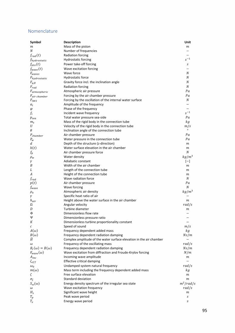
95

Nomenclature

Symbol Description Unit 𝑚 Mass of the piston 𝑚 𝑁 Number of frequencies − 𝑓𝑟𝑎𝑑(𝑡) Radiation forcing − 𝑓ℎ𝑦𝑑𝑟𝑜𝑠𝑡𝑎𝑡𝑖𝑐 Hydrostatic forcing 𝑠−1

𝑓𝑝𝑡𝑜(𝑡) Power take-off forcing 𝑠

𝑓𝑤𝑎𝑣𝑒(𝑡) Wave excitation forcing − 𝐹𝑤𝑎𝑣𝑒𝑠 Wave force 𝑁 𝐹ℎ𝑦𝑑𝑟𝑜𝑠𝑡𝑎𝑡𝑖𝑐 Hydrostatic force 𝑁

𝐹𝑔,𝜃 Gravity force incl. the inclination angle 𝑁

𝐹𝑟𝑎𝑑 Radiation forcing 𝑁 𝐹𝑎𝑡𝑚𝑜𝑠𝑝ℎ𝑒𝑟𝑖𝑐 Atmospheric air pressure 𝑃𝑎

𝐹𝑎𝑖𝑟 𝑐ℎ𝑎𝑚𝑏𝑒𝑟 Forcing by the air chamber pressure 𝑃𝑎 𝐹𝐼𝑊𝑆 Forcing by the oscillation of the internal water surface 𝑁 𝑎𝑖 Amplitude of the frequency − 𝜑 Phase of the frequency − 𝑓𝑖 Incident wave frequency 𝑠−1 𝑝𝑠𝑒𝑎 Total water pressure sea-side 𝑃𝑎 𝑚𝑡 Mass of the rigid body in the connection tube 𝑘𝑔 𝑈 Velocity of the rigid body in the connection tube 𝑚/𝑠 휃 Inclination angle of the connection tube ° 𝑃𝑐ℎ𝑎𝑚𝑏𝑒𝑟 Air chamber pressure 𝑃𝑎

𝑃𝑤 Water pressure in the connection tube 𝑃𝑎 𝑑 Depth of the structure (z-direction) 𝑚

ℎ(𝑡) Water surface elevation in the air chamber 𝑚 𝑓𝑝 Air chamber pressure force 𝑁

𝜌𝑤 Water density 𝑘𝑔/𝑚3 𝛾 Adiabatic constant [−] 𝐵 Width of the air chamber 𝑚 𝐿 Length of the connection tube 𝑚 𝐴 Height of the connection tube 𝑚 𝑓𝑟𝑎𝑑 Wave radiation force 𝑁 𝑝(𝑡) Air chamber pressure 𝑃𝑎 𝑓𝑤𝑎𝑣𝑒 Wave forcing 𝑁 𝜌𝑎 Atmospheric air density 𝑘𝑔/𝑚3 𝛾 Specific heat ratio of air − ℎ𝑎𝑖𝑟 Height above the water surface in the air chamber 𝑚 Ω Angular velocity 𝑟𝑎𝑑/𝑠 𝐷 Turbine diameter 𝑚 Φ Dimensionless flow rate − Ψ Dimensionless pressure ratio − 𝐾 Dimensionless turbine proportionality constant − 𝑐 Speed of sound 𝑚/𝑠 𝐴(𝜔) Frequency dependent added mass 𝑘𝑔 𝐵(𝜔) Frequency dependent radiation damping 𝑁𝑠/𝑚

�� Complex amplitude of the water surface elevation in the air chamber − 𝜔 Frequency of the oscillating mass 𝑟𝑎𝑑/𝑠 𝐵𝑟(𝜔) = 𝐵(𝜔) Frequency dependent radiation damping 𝑁𝑠/𝑚 𝐹𝑤𝑎𝑣𝑒(𝜔) Wave excitation from diffraction and Froude-Krylov forcing 𝑁/𝑚 𝐴𝑖𝑛𝑐 Incoming wave amplitude 𝑚 휁𝑒𝑓𝑓 Effective critical damping −

𝜔0 Undamped system natural frequency 𝑟𝑎𝑑/𝑠 𝑚(𝜔) Mass term including the frequency dependent added mass 𝑘𝑔 휁 Free surface elevation 𝑚 𝜎𝜁 Standard deviation 𝑚

𝑆ω(ω) Energy density spectrum of the irregular sea state 𝑚2/𝑟𝑎𝑑/𝑠 𝜔 Wave excitation frequency 𝑟𝑎𝑑/𝑠 𝐻𝑠 Significant wave height 𝑚 𝑇𝑝 Peak wave period 𝑠

𝑇𝑒 Energy wave period 𝑠

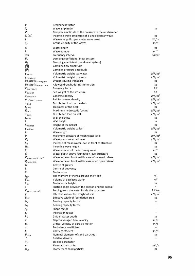
96

𝛾 Peakedness factor − 휁𝑎 Wave amplitude 𝑚

�� Complex amplitude of the pressure in the air chamber − 휁𝑎(𝜔) Incoming wave amplitude of a single regular wave 𝑚 𝐽 Wave energy flux per meter wave crest 𝑊/𝑚 𝑐𝑔 Group velocity of the waves 𝑚/𝑠

𝑑 Water depth 𝑚 𝑘 Wave number 𝑚−1 𝑑𝜔 Frequency interval 𝑟𝑎𝑑/𝑠 𝐵1 Damping coefficient (linear system) 𝐵2 Damping coefficient (non-linear system)

|𝑄| Complex flow amplitude

|𝑃| Complex pressure amplitude

𝛾𝑤𝑎𝑡𝑒𝑟 Volumetric weight sea water 𝑘𝑁/𝑚3 𝛾𝑐𝑜𝑛𝑐𝑟𝑒𝑡𝑒 Volumetric weight concrete 𝑘𝑁/𝑚3 𝐷𝑟𝑎𝑢𝑔ℎ𝑡𝑡𝑟𝑎𝑛𝑠𝑝𝑜𝑟𝑡 Draught during transport 𝑚

𝐷𝑟𝑎𝑢𝑔ℎ𝑡𝑖𝑚𝑚𝑒𝑟𝑠𝑖𝑜𝑛 Allowed draught during immersion 𝑚 𝐹𝑏𝑢𝑜𝑦𝑎𝑛𝑐𝑦 Buoyancy force 𝑘𝑁

𝐹𝑤𝑒𝑖𝑔ℎ𝑡 Self weight of the structure 𝑘𝑁

𝜌𝑐𝑜𝑛𝑐𝑟𝑒𝑡𝑒 Concrete density 𝑘𝑁/𝑚3 𝜌𝑟𝑒𝑖𝑛𝑓𝑜𝑟𝑐𝑒𝑚𝑒𝑛𝑡 Reinforcement density 𝑘𝑁/𝑚3

𝑞𝑑𝑒𝑐𝑘 Distributed load on the deck 𝑘𝑁/𝑚2 𝑡𝑑𝑒𝑐𝑘 Thickness of the deck 𝑚 𝑃𝑚𝑎𝑥 Maximum hydrostatic forcing 𝑘𝑁/𝑚2 𝑞𝑤𝑎𝑙𝑙 Distributed load on wall 𝑘𝑁/𝑚2 𝑡𝑤𝑎𝑙𝑙 Wall thickness 𝑚 ℎ Wall height 𝑚 ℎ𝑏𝑎𝑙𝑙𝑎𝑠𝑡 Height of the ballast 𝑚 𝛾𝑏𝑎𝑙𝑙𝑎𝑠𝑡 Volumetric weight ballast 𝑘𝑁/𝑚3 𝐿 Wavelength 𝑚 𝑃1 Maximum pressure at mean water level 𝑘𝑁/𝑚2 𝑃0 Wave pressure at bed level 𝑘𝑁/𝑚2 ℎ0 Increase of mean water level in front of structure 𝑚 𝐻𝑖𝑛 Incoming wave height 𝑚 𝑘 Wave number of the incoming wave 𝑚−1 𝑑′ Water depth above foundation level structure 𝑚 𝑃𝑚𝑎𝑥,𝑐𝑙𝑜𝑠𝑒𝑑−𝑜𝑓𝑓 Wave force on front wall in case of a closed caisson 𝑘𝑁/𝑚2

𝑃𝑚𝑎𝑥,𝑜𝑝𝑒𝑛 Wave force on front wall in case of an open caisson 𝑘𝑁/𝑚2

G Centre of gravity B Centre of buoyancy M Metacenter 𝐼𝑦𝑦 The moment of inertia around the y-axis 𝑚4

𝑉𝑑𝑤 Volume of displaced water 𝑚3 ℎ𝑚 Metacentric height 𝑚 𝛿 Friction angle between the caisson and the subsoil ° 𝐹𝑤𝑎𝑡𝑒𝑟−𝑖𝑛𝑠𝑖𝑑𝑒 Forcing from the water inside the structure 𝑘𝑁/𝑚 𝛾′ Effective volumetric weight of soil 𝑘𝑁/𝑚3 Beff Effective width of foundation area 𝑚 𝑁𝛾 Bearing capacity factor −

𝑁𝑞 Bearing capacity factor −

𝑠𝛾 Shape factor −

𝑖𝛾 Inclination factor −

ℎ0 (Initial) water depth 𝑚 𝑢 Depth-averaged flow velocity 𝑚/𝑠 𝑢𝑐 Critical velocity of particle motion 𝑚/𝑠 𝛼 Turbulence coefficient − 𝐶 Chézy coefficient 𝑚/𝑠 𝐷𝑛50 Nominal diameter of sand particles 𝑚 ∆ Relative density − 𝛹𝑐 Shields parameter − 𝑣 Kinematic viscosity 𝑚2/𝑠 𝐷50 Diameter of sand particles 𝑚

97

𝛾𝑠𝑎𝑓𝑒𝑡𝑦 Safety factor = 1.0 −

𝑛𝑠 1/𝑛𝑠 is the average slope of the slide − 𝑀𝑟𝑑 Moment capacity 𝑘𝑁𝑚/𝑚 𝑉𝑟𝑑 Shear force capacity 𝑘𝑁/𝑚 ∅ Diameter reinforcement 𝑚𝑚 𝑐 Concrete cover 𝑚𝑚

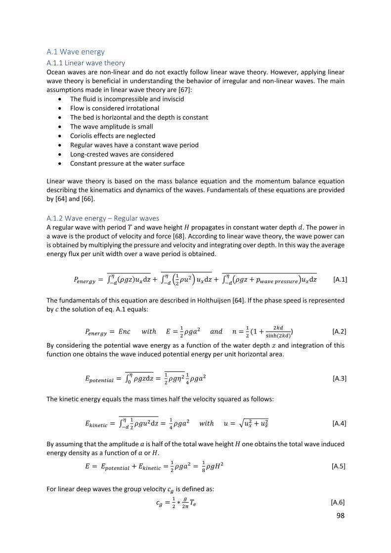
98

𝑃𝑒𝑛𝑒𝑟𝑔𝑦 = ∫ (𝜌𝑔𝑧)𝑢𝑥d𝑧𝜂

−𝑑+ ∫ (

1

2𝜌𝑢2) 𝑢𝑥d𝑧

𝜂

−𝑑+ ∫ (𝜌𝑔𝑧 + 𝑝𝑤𝑎𝑣𝑒 𝑝𝑟𝑒𝑠𝑠𝑢𝑟𝑒)𝑢𝑥d𝑧

𝜂

−𝑑 [A.1]

[2.2]

𝑃𝑒𝑛𝑒𝑟𝑔𝑦 = 𝐸𝑛𝑐 𝑤𝑖𝑡ℎ 𝐸 =1

2𝜌𝑔𝑎2 𝑎𝑛𝑑 𝑛 =

1

2(1 +

2𝑘𝑑

sinh (2𝑘𝑑)) [A.2]

[2.2]

𝐸𝑝𝑜𝑡𝑒𝑛𝑡𝑖𝑎𝑙 = ∫ 𝜌𝑔𝑧d𝑧

𝜂

0=

1

2𝜌𝑔휂2 1

4𝜌𝑔𝑎2 [A.3]

[2.2]

𝐸𝑘𝑖𝑛𝑒𝑡𝑖𝑐 = ∫

1

2𝜌𝑔𝑢2d𝑧

𝜂

−𝑑=

1

4𝜌𝑔𝑎2 𝑤𝑖𝑡ℎ 𝑢 = √𝑢𝑥

2 + 𝑢𝑧2 [A.4]

[2.2]

𝐸 = 𝐸𝑝𝑜𝑡𝑒𝑛𝑡𝑖𝑎𝑙 + 𝐸𝑘𝑖𝑛𝑒𝑡𝑖𝑐 =

1

2𝜌𝑔𝑎2 =

1

8𝜌𝑔𝐻2 [A.5]

[2.2]

𝑐𝑔 =1

2∗

𝑔

2𝜋𝑇𝑒 [A.6]

[2.2]

A.1 Wave energy

A.1.1 Linear wave theory Ocean waves are non-linear and do not exactly follow linear wave theory. However, applying linear wave theory is beneficial in understanding the behavior of irregular and non-linear waves. The main assumptions made in linear wave theory are [67]:

• The fluid is incompressible and inviscid

• Flow is considered irrotational

• The bed is horizontal and the depth is constant

• The wave amplitude is small

• Coriolis effects are neglected

• Regular waves have a constant wave period

• Long-crested waves are considered

• Constant pressure at the water surface Linear wave theory is based on the mass balance equation and the momentum balance equation describing the kinematics and dynamics of the waves. Fundamentals of these equations are provided by [64] and [66].

A.1.2 Wave energy – Regular waves A regular wave with period 𝑇 and wave height 𝐻 propagates in constant water depth 𝑑. The power in a wave is the product of velocity and force [68]. According to linear wave theory, the wave power can is obtained by multiplying the pressure and velocity and integrating over depth. In this way the average energy flux per unit width over a wave period is obtained.

The fundamentals of this equation are described in Holthuijsen [64]. If the phase speed is represented by 𝑐 the solution of eq. A.1 equals:

By considering the potential wave energy as a function of the water depth 𝑧 and integration of this function one obtains the wave induced potential energy per unit horizontal area.

The kinetic energy equals the mass times half the velocity squared as follows:

By assuming that the amplitude 𝑎 is half of the total wave height 𝐻 one obtains the total wave induced energy density as a function of 𝑎 or 𝐻.

For linear deep waves the group velocity 𝑐𝑔 is defined as:

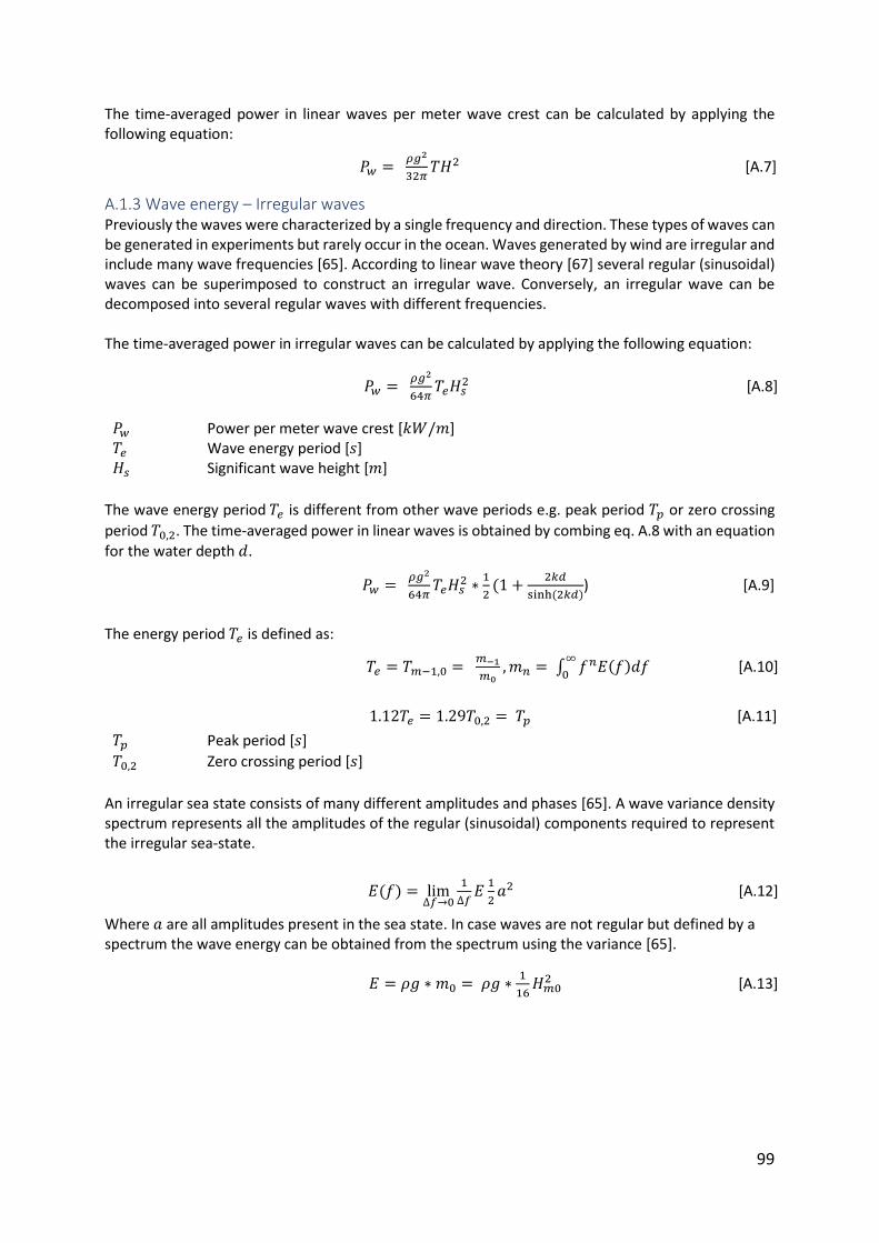
99

𝑃𝑤 = 𝜌𝑔2

32𝜋𝑇𝐻2 [A.7]

[2.2]

𝑃𝑤 = 𝜌𝑔2

64𝜋𝑇𝑒𝐻𝑠

2 [A.8]

[2.2]

𝑃𝑤 = 𝜌𝑔2

64𝜋𝑇𝑒𝐻𝑠

2 ∗1

2(1 +

2𝑘𝑑

sinh (2𝑘𝑑)) [A.9]

[2.2]

𝑇𝑒 = 𝑇𝑚−1,0 = 𝑚−1

𝑚0, 𝑚𝑛 = ∫ 𝑓𝑛𝐸(𝑓)𝑑𝑓

∞

0 [A.10]

[2.2]

1.12𝑇𝑒 = 1.29𝑇0,2 = 𝑇𝑝 [A.11]

[2.2]

𝐸(𝑓) = lim∆𝑓→0

1

∆𝑓𝐸

1

2𝑎2 [A.12]

[2.2]

𝐸 = 𝜌𝑔 ∗ 𝑚0 = 𝜌𝑔 ∗1

16𝐻𝑚0

2 [A.13]

[2.2]

The time-averaged power in linear waves per meter wave crest can be calculated by applying the following equation:

A.1.3 Wave energy – Irregular waves Previously the waves were characterized by a single frequency and direction. These types of waves can be generated in experiments but rarely occur in the ocean. Waves generated by wind are irregular and include many wave frequencies [65]. According to linear wave theory [67] several regular (sinusoidal) waves can be superimposed to construct an irregular wave. Conversely, an irregular wave can be decomposed into several regular waves with different frequencies. The time-averaged power in irregular waves can be calculated by applying the following equation:

𝑃𝑤 Power per meter wave crest [𝑘𝑊/𝑚] 𝑇𝑒 Wave energy period [𝑠] 𝐻𝑠 Significant wave height [𝑚]

The wave energy period 𝑇𝑒 is different from other wave periods e.g. peak period 𝑇𝑝 or zero crossing

period 𝑇0,2. The time-averaged power in linear waves is obtained by combing eq. A.8 with an equation for the water depth 𝑑.

The energy period 𝑇𝑒 is defined as:

𝑇𝑝 Peak period [𝑠]

𝑇0,2 Zero crossing period [𝑠]

An irregular sea state consists of many different amplitudes and phases [65]. A wave variance density spectrum represents all the amplitudes of the regular (sinusoidal) components required to represent the irregular sea-state.

Where 𝑎 are all amplitudes present in the sea state. In case waves are not regular but defined by a spectrum the wave energy can be obtained from the spectrum using the variance [65].

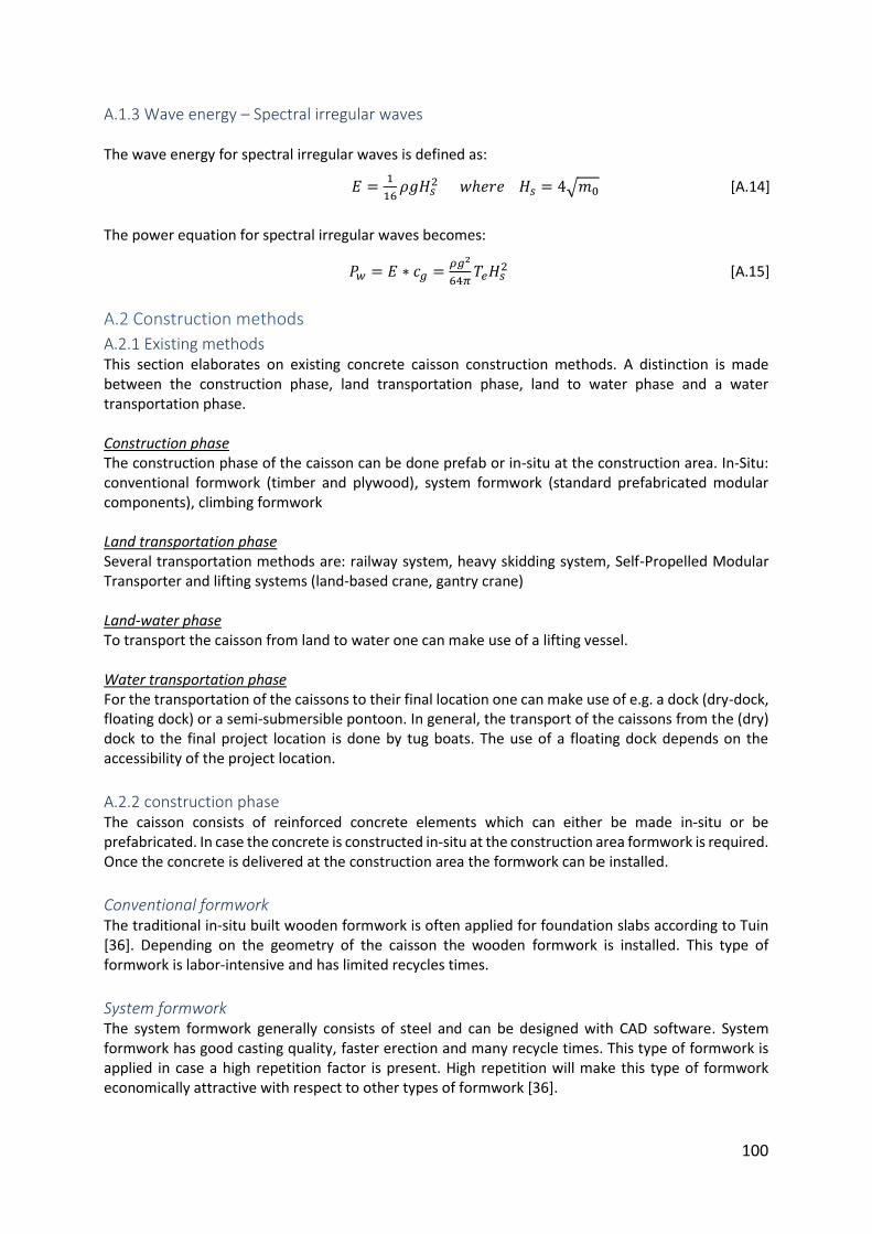
100

𝐸 =1

16𝜌𝑔𝐻𝑠

2 𝑤ℎ𝑒𝑟𝑒 𝐻𝑠 = 4√𝑚0 [A.14]

[2.2]

𝑃𝑤 = 𝐸 ∗ 𝑐𝑔 =𝜌𝑔2

64𝜋𝑇𝑒𝐻𝑠

2 [A.15]

[2.2]

A.1.3 Wave energy – Spectral irregular waves The wave energy for spectral irregular waves is defined as:

The power equation for spectral irregular waves becomes:

A.2 Construction methods

A.2.1 Existing methods This section elaborates on existing concrete caisson construction methods. A distinction is made between the construction phase, land transportation phase, land to water phase and a water transportation phase. Construction phase The construction phase of the caisson can be done prefab or in-situ at the construction area. In-Situ: conventional formwork (timber and plywood), system formwork (standard prefabricated modular components), climbing formwork Land transportation phase Several transportation methods are: railway system, heavy skidding system, Self-Propelled Modular Transporter and lifting systems (land-based crane, gantry crane) Land-water phase To transport the caisson from land to water one can make use of a lifting vessel. Water transportation phase For the transportation of the caissons to their final location one can make use of e.g. a dock (dry-dock, floating dock) or a semi-submersible pontoon. In general, the transport of the caissons from the (dry) dock to the final project location is done by tug boats. The use of a floating dock depends on the accessibility of the project location.

A.2.2 construction phase The caisson consists of reinforced concrete elements which can either be made in-situ or be prefabricated. In case the concrete is constructed in-situ at the construction area formwork is required. Once the concrete is delivered at the construction area the formwork can be installed.

Conventional formwork The traditional in-situ built wooden formwork is often applied for foundation slabs according to Tuin [36]. Depending on the geometry of the caisson the wooden formwork is installed. This type of formwork is labor-intensive and has limited recycles times.

System formwork The system formwork generally consists of steel and can be designed with CAD software. System formwork has good casting quality, faster erection and many recycle times. This type of formwork is applied in case a high repetition factor is present. High repetition will make this type of formwork economically attractive with respect to other types of formwork [36].

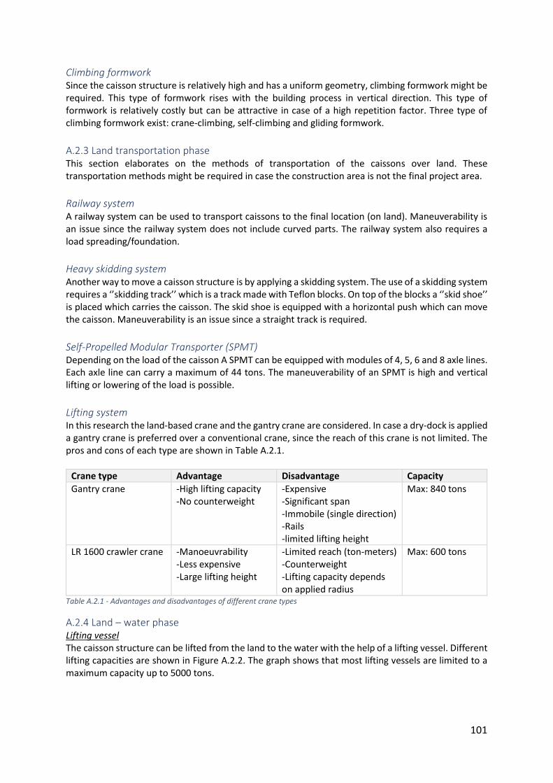
101

Climbing formwork Since the caisson structure is relatively high and has a uniform geometry, climbing formwork might be required. This type of formwork rises with the building process in vertical direction. This type of formwork is relatively costly but can be attractive in case of a high repetition factor. Three type of climbing formwork exist: crane-climbing, self-climbing and gliding formwork.

A.2.3 Land transportation phase This section elaborates on the methods of transportation of the caissons over land. These transportation methods might be required in case the construction area is not the final project area.

Railway system A railway system can be used to transport caissons to the final location (on land). Maneuverability is an issue since the railway system does not include curved parts. The railway system also requires a load spreading/foundation.

Heavy skidding system Another way to move a caisson structure is by applying a skidding system. The use of a skidding system requires a ‘’skidding track’’ which is a track made with Teflon blocks. On top of the blocks a ‘’skid shoe’’ is placed which carries the caisson. The skid shoe is equipped with a horizontal push which can move the caisson. Maneuverability is an issue since a straight track is required.

Self-Propelled Modular Transporter (SPMT) Depending on the load of the caisson A SPMT can be equipped with modules of 4, 5, 6 and 8 axle lines. Each axle line can carry a maximum of 44 tons. The maneuverability of an SPMT is high and vertical lifting or lowering of the load is possible.

Lifting system In this research the land-based crane and the gantry crane are considered. In case a dry-dock is applied a gantry crane is preferred over a conventional crane, since the reach of this crane is not limited. The pros and cons of each type are shown in Table A.2.1.

Crane type Advantage Disadvantage Capacity

Gantry crane -High lifting capacity -No counterweight

-Expensive -Significant span -Immobile (single direction) -Rails -limited lifting height

Max: 840 tons

LR 1600 crawler crane -Manoeuvrability -Less expensive -Large lifting height

-Limited reach (ton-meters) -Counterweight -Lifting capacity depends on applied radius

Max: 600 tons

Table A.2.1 - Advantages and disadvantages of different crane types

A.2.4 Land – water phase Lifting vessel The caisson structure can be lifted from the land to the water with the help of a lifting vessel. Different lifting capacities are shown in Figure A.2.2. The graph shows that most lifting vessels are limited to a maximum capacity up to 5000 tons.

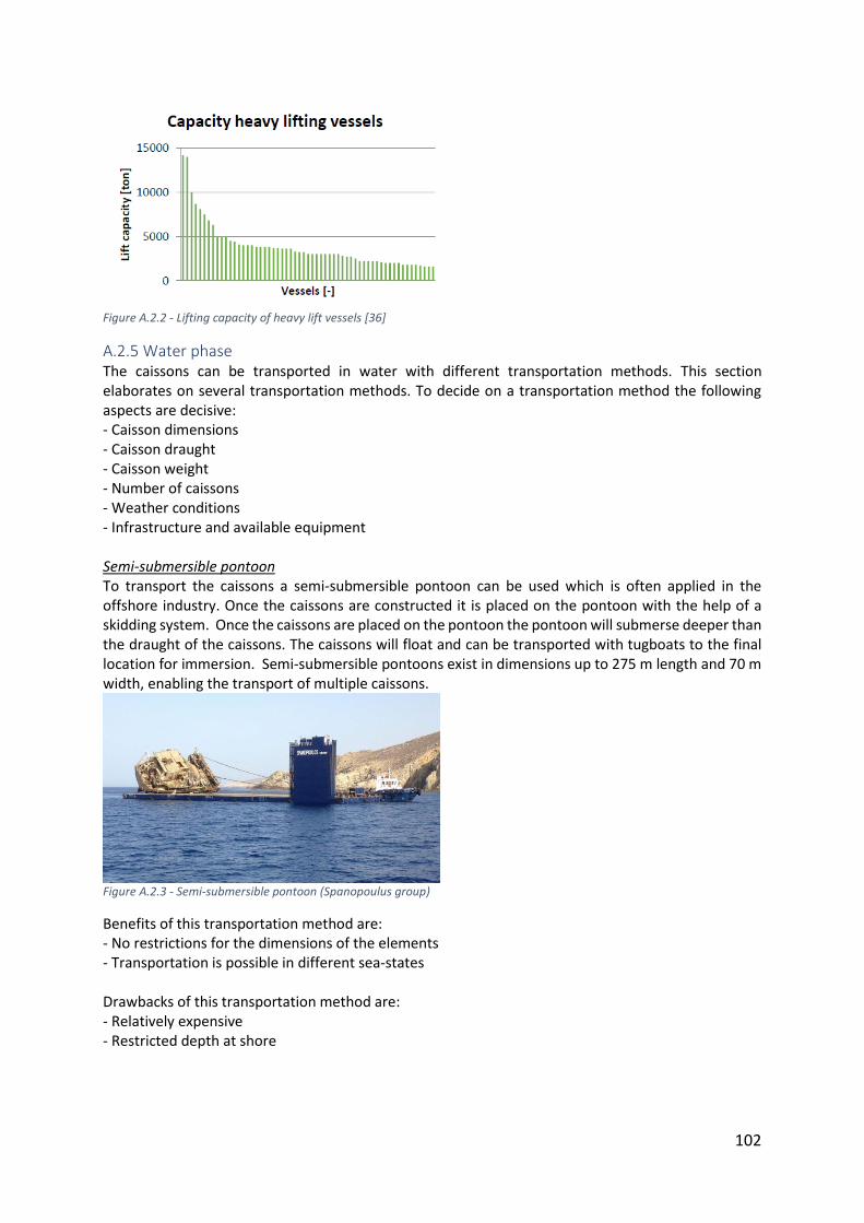
102

Figure A.2.2 - Lifting capacity of heavy lift vessels [36]

A.2.5 Water phase The caissons can be transported in water with different transportation methods. This section elaborates on several transportation methods. To decide on a transportation method the following aspects are decisive: - Caisson dimensions - Caisson draught - Caisson weight - Number of caissons - Weather conditions - Infrastructure and available equipment Semi-submersible pontoon To transport the caissons a semi-submersible pontoon can be used which is often applied in the offshore industry. Once the caissons are constructed it is placed on the pontoon with the help of a skidding system. Once the caissons are placed on the pontoon the pontoon will submerse deeper than the draught of the caissons. The caissons will float and can be transported with tugboats to the final location for immersion. Semi-submersible pontoons exist in dimensions up to 275 m length and 70 m width, enabling the transport of multiple caissons.

Figure A.2.3 - Semi-submersible pontoon (Spanopoulus group)

Benefits of this transportation method are: - No restrictions for the dimensions of the elements - Transportation is possible in different sea-states Drawbacks of this transportation method are: - Relatively expensive - Restricted depth at shore

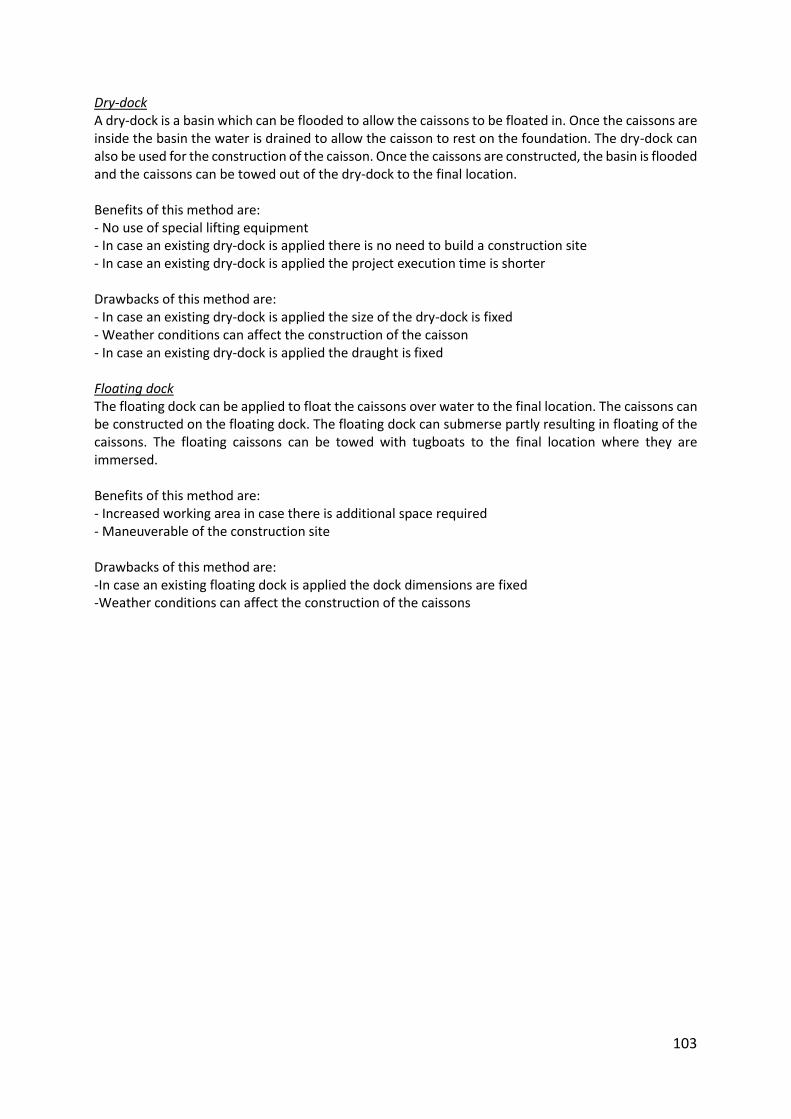
103

Dry-dock A dry-dock is a basin which can be flooded to allow the caissons to be floated in. Once the caissons are inside the basin the water is drained to allow the caisson to rest on the foundation. The dry-dock can also be used for the construction of the caisson. Once the caissons are constructed, the basin is flooded and the caissons can be towed out of the dry-dock to the final location. Benefits of this method are: - No use of special lifting equipment - In case an existing dry-dock is applied there is no need to build a construction site - In case an existing dry-dock is applied the project execution time is shorter Drawbacks of this method are: - In case an existing dry-dock is applied the size of the dry-dock is fixed - Weather conditions can affect the construction of the caisson - In case an existing dry-dock is applied the draught is fixed Floating dock The floating dock can be applied to float the caissons over water to the final location. The caissons can be constructed on the floating dock. The floating dock can submerse partly resulting in floating of the caissons. The floating caissons can be towed with tugboats to the final location where they are immersed. Benefits of this method are: - Increased working area in case there is additional space required - Maneuverable of the construction site Drawbacks of this method are: -In case an existing floating dock is applied the dock dimensions are fixed -Weather conditions can affect the construction of the caissons

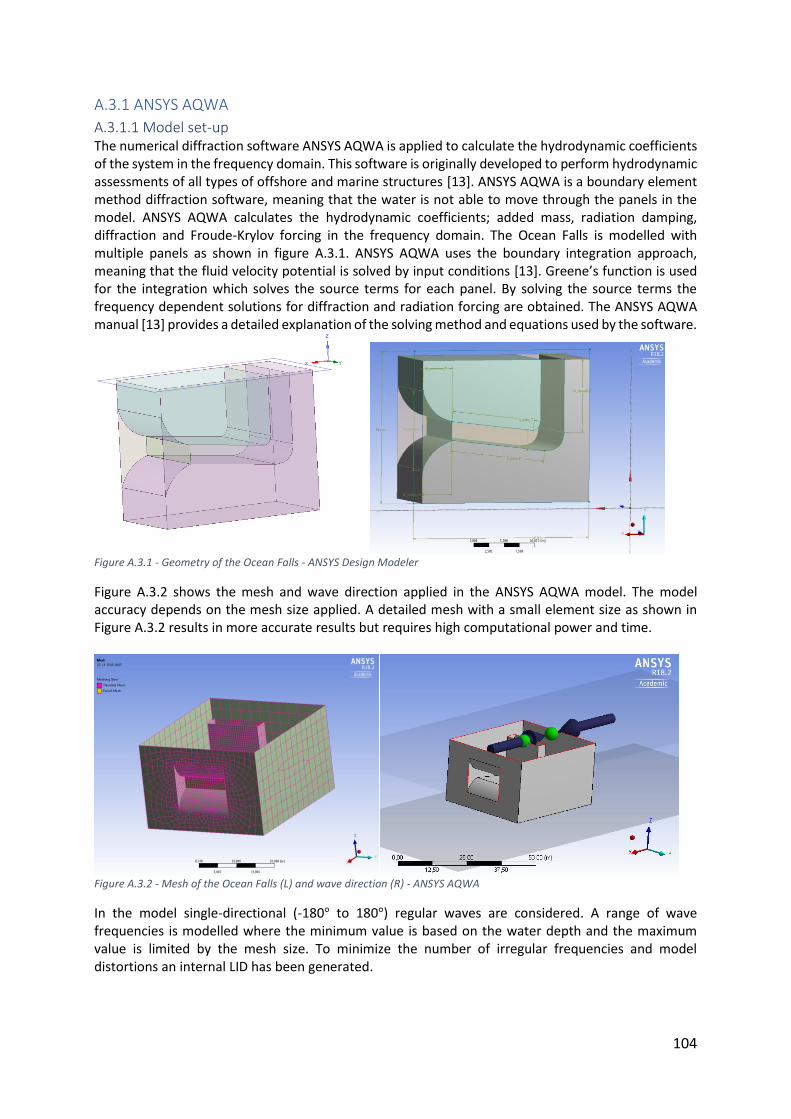
104

A.3.1 ANSYS AQWA

A.3.1.1 Model set-up The numerical diffraction software ANSYS AQWA is applied to calculate the hydrodynamic coefficients of the system in the frequency domain. This software is originally developed to perform hydrodynamic assessments of all types of offshore and marine structures [13]. ANSYS AQWA is a boundary element method diffraction software, meaning that the water is not able to move through the panels in the model. ANSYS AQWA calculates the hydrodynamic coefficients; added mass, radiation damping, diffraction and Froude-Krylov forcing in the frequency domain. The Ocean Falls is modelled with multiple panels as shown in figure A.3.1. ANSYS AQWA uses the boundary integration approach, meaning that the fluid velocity potential is solved by input conditions [13]. Greene’s function is used for the integration which solves the source terms for each panel. By solving the source terms the frequency dependent solutions for diffraction and radiation forcing are obtained. The ANSYS AQWA manual [13] provides a detailed explanation of the solving method and equations used by the software.

Figure A.3.1 - Geometry of the Ocean Falls - ANSYS Design Modeler

Figure A.3.2 shows the mesh and wave direction applied in the ANSYS AQWA model. The model accuracy depends on the mesh size applied. A detailed mesh with a small element size as shown in Figure A.3.2 results in more accurate results but requires high computational power and time.

Figure A.3.2 - Mesh of the Ocean Falls (L) and wave direction (R) - ANSYS AQWA

In the model single-directional (-180° to 180°) regular waves are considered. A range of wave frequencies is modelled where the minimum value is based on the water depth and the maximum value is limited by the mesh size. To minimize the number of irregular frequencies and model distortions an internal LID has been generated.

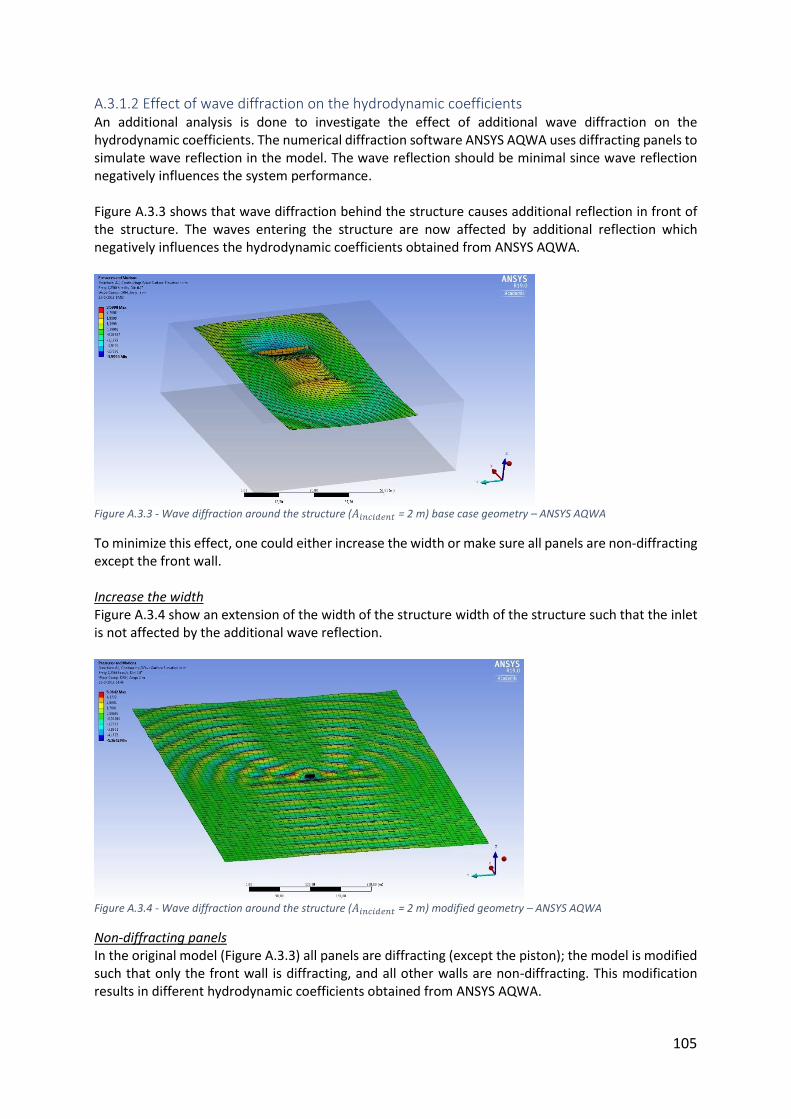
105

A.3.1.2 Effect of wave diffraction on the hydrodynamic coefficients An additional analysis is done to investigate the effect of additional wave diffraction on the hydrodynamic coefficients. The numerical diffraction software ANSYS AQWA uses diffracting panels to simulate wave reflection in the model. The wave reflection should be minimal since wave reflection negatively influences the system performance. Figure A.3.3 shows that wave diffraction behind the structure causes additional reflection in front of the structure. The waves entering the structure are now affected by additional reflection which negatively influences the hydrodynamic coefficients obtained from ANSYS AQWA.

Figure A.3.3 - Wave diffraction around the structure (𝐴𝑖𝑛𝑐𝑖𝑑𝑒𝑛𝑡 = 2 m) base case geometry – ANSYS AQWA

To minimize this effect, one could either increase the width or make sure all panels are non-diffracting except the front wall. Increase the width Figure A.3.4 show an extension of the width of the structure width of the structure such that the inlet is not affected by the additional wave reflection.

Figure A.3.4 - Wave diffraction around the structure (𝐴𝑖𝑛𝑐𝑖𝑑𝑒𝑛𝑡 = 2 m) modified geometry – ANSYS AQWA

Non-diffracting panels In the original model (Figure A.3.3) all panels are diffracting (except the piston); the model is modified such that only the front wall is diffracting, and all other walls are non-diffracting. This modification results in different hydrodynamic coefficients obtained from ANSYS AQWA.

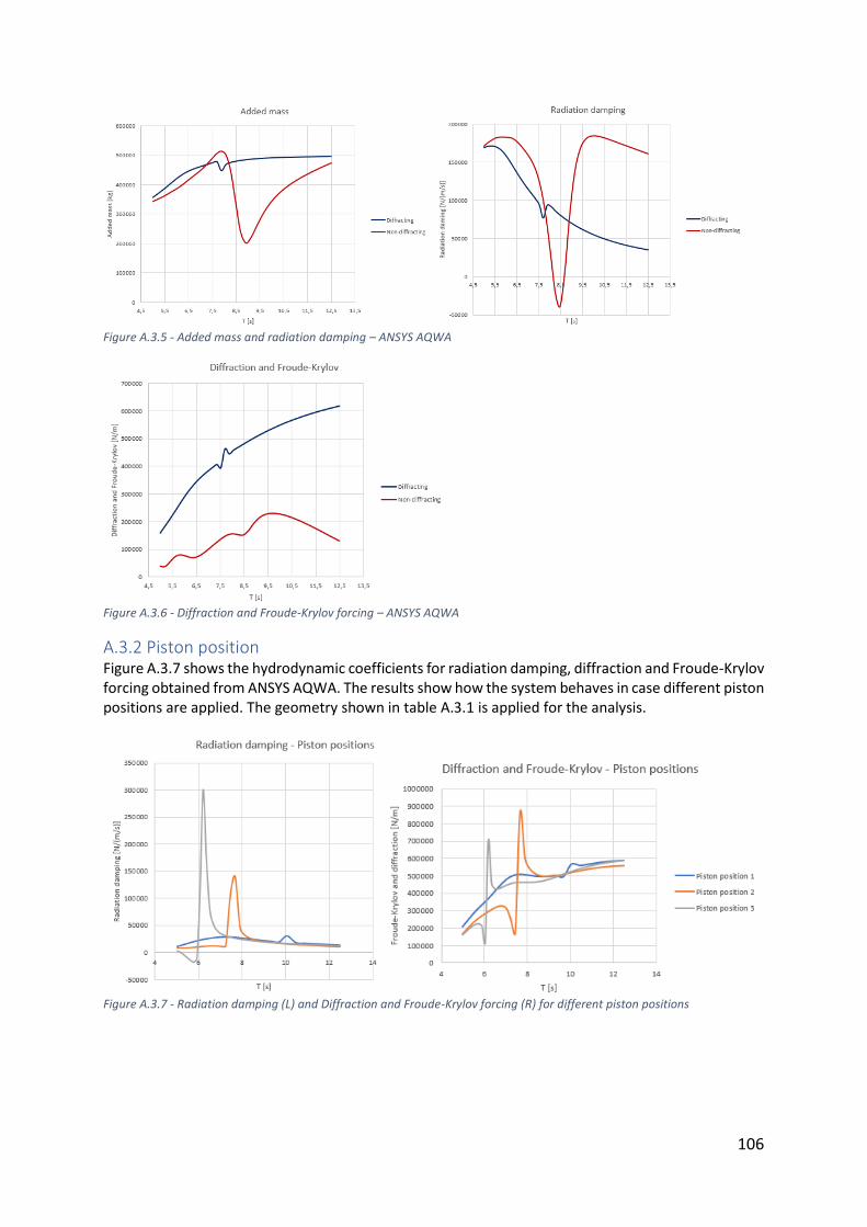
106

Figure A.3.5 - Added mass and radiation damping – ANSYS AQWA

Figure A.3.6 - Diffraction and Froude-Krylov forcing – ANSYS AQWA

A.3.2 Piston position Figure A.3.7 shows the hydrodynamic coefficients for radiation damping, diffraction and Froude-Krylov forcing obtained from ANSYS AQWA. The results show how the system behaves in case different piston positions are applied. The geometry shown in table A.3.1 is applied for the analysis.

Figure A.3.7 - Radiation damping (L) and Diffraction and Froude-Krylov forcing (R) for different piston positions

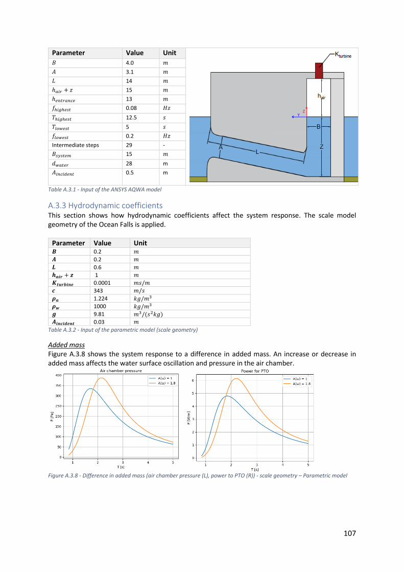
107

Parameter Value Unit

𝐵 4.0 𝑚

𝐴 3.1 𝑚

𝐿 14 𝑚

ℎ𝑎𝑖𝑟 + 𝑧 15 𝑚

ℎ𝑒𝑛𝑡𝑟𝑎𝑛𝑐𝑒 13 𝑚

𝑓ℎ𝑖𝑔ℎ𝑒𝑠𝑡 0.08 𝐻𝑧

𝑇ℎ𝑖𝑔ℎ𝑒𝑠𝑡 12.5 𝑠

𝑇𝑙𝑜𝑤𝑒𝑠𝑡 5 𝑠

𝑓𝑙𝑜𝑤𝑒𝑠𝑡 0.2 𝐻𝑧

Intermediate steps 29 -

𝐵𝑠𝑦𝑠𝑡𝑒𝑚 15 𝑚

𝑑𝑤𝑎𝑡𝑒𝑟 28 m

𝐴𝑖𝑛𝑐𝑖𝑑𝑒𝑛𝑡 0.5 m

Table A.3.1 - Input of the ANSYS AQWA model

A.3.3 Hydrodynamic coefficients This section shows how hydrodynamic coefficients affect the system response. The scale model geometry of the Ocean Falls is applied.

Parameter Value Unit 𝑩 0.2 𝑚

𝑨 0.2 𝑚

𝑳 0.6 𝑚

𝒉𝒂𝒊𝒓 + 𝒛 1 𝑚

𝑲𝒕𝒖𝒓𝒃𝒊𝒏𝒆 0.0001 𝑚𝑠/𝑚

𝒄 343 𝑚/𝑠

𝝆𝒂 1.224 𝑘𝑔/𝑚3

𝝆𝒘 1000 𝑘𝑔/𝑚3 𝒈 9.81 𝑚3/(𝑠2𝑘𝑔) 𝑨𝒊𝒏𝒄𝒊𝒅𝒆𝒏𝒕 0.03 𝑚

Table A.3.2 - Input of the parametric model (scale geometry)

Added mass Figure A.3.8 shows the system response to a difference in added mass. An increase or decrease in added mass affects the water surface oscillation and pressure in the air chamber.

Figure A.3.8 - Difference in added mass (air chamber pressure (L), power to PTO (R)) - scale geometry – Parametric model

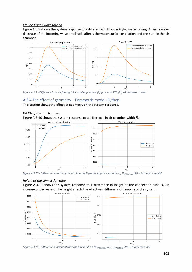
108

Froude-Krylov wave forcing Figure A.3.9 shows the system response to a difference in Froude-Krylov wave forcing. An increase or decrease of the incoming wave amplitude affects the water surface oscillation and pressure in the air chamber.

Figure A.3.9 - Difference in wave forcing (air chamber pressure (L), power to PTO (R)) – Parametric model

A.3.4 The effect of geometry – Parametric model (Python) This section shows the effect of geometry on the system response. Width of the air chamber Figure A.3.10 shows the system response to a difference in air chamber width 𝐵.

Figure A.3.10 - Difference in width of the air chamber B (water surface elevation (L), 𝐵𝑒𝑓𝑓𝑒𝑐𝑡𝑖𝑣𝑒(R)) – Parametric model

Height of the connection tube Figure A.3.11 shows the system response to a difference in height of the connection tube 𝐴. An increase or decrease of the height affects the effective- stiffness and damping of the system.

Figure A.3.11 - Difference in height of the connection tube A (𝐾𝑒𝑓𝑓𝑒𝑐𝑡𝑖𝑣𝑒 (L), 𝐵𝑒𝑓𝑓𝑒𝑐𝑡𝑖𝑣𝑒(R)) – Parametric model

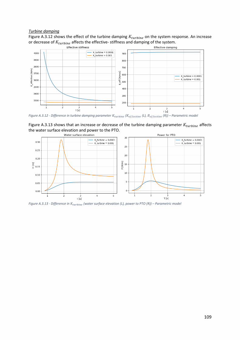
109

Turbine damping Figure A.3.12 shows the effect of the turbine damping 𝐾𝑡𝑢𝑟𝑏𝑖𝑛𝑒 on the system response. An increase or decrease of 𝐾𝑡𝑢𝑟𝑏𝑖𝑛𝑒 affects the effective- stiffness and damping of the system.

Figure A.3.12 - Difference in turbine damping parameter 𝐾𝑡𝑢𝑟𝑏𝑖𝑛𝑒 (𝐾𝑒𝑓𝑓𝑒𝑐𝑡𝑖𝑣𝑒 (L), 𝐵𝑒𝑓𝑓𝑒𝑐𝑡𝑖𝑣𝑒 (R)) – Parametric model

Figure A.3.13 shows that an increase or decrease of the turbine damping parameter 𝐾𝑡𝑢𝑟𝑏𝑖𝑛𝑒 affects the water surface elevation and power to the PTO.

Figure A.3.13 - Difference in 𝐾𝑡𝑢𝑟𝑏𝑖𝑛𝑒 (water surface elevation (L), power to PTO (R)) – Parametric model

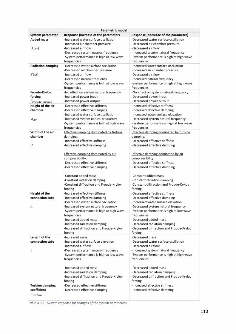
110

Parametric model

System parameter Response (increase of the parameter) Response (decrease of the parameter)

Added mass 𝐴(𝜔)

-Increased water surface oscillation -Increased air chamber pressure -Increased air flow -Decreased system natural frequency -System performance is high at low wave frequencies

-Decreased water surface oscillation -Decreased air chamber pressure -Decreased air flow -Increased system natural frequency -System performance is high at high wave frequencies

Radiation damping 𝐵(𝜔)

-Decreased water surface oscillation -Decreased air chamber pressure -Increased air flow -Decreased natural frequency -System performance is high at low wave frequencies

-Increased water surface oscillation -Increased air chamber pressure -Decreased air flow -Increased natural frequency -System performance is high at high wave frequencies

Froude-Krylov forcing 𝐹𝐹𝑟𝑜𝑢𝑑𝑒−𝐾𝑟𝑦𝑙𝑜𝑣

-No effect on system natural frequency -Increased power input -Increased power output

-No effect on system natural frequency -Decreased power input -Decreased power output

Height of the air chamber ℎ𝑎𝑖𝑟

-Decreased effective stiffness -Decreased effective damping -Increased water surface oscillation -Increased system natural frequency -System performance is high at high wave frequencies

-Increased effective stiffness -Increased effective damping -Increased water surface elevation -Decreased system natural frequency - System performance is high at low wave frequencies

Width of the air chamber 𝐵

Effective damping dominated by turbine damping: -Increased effective stiffness -Increased effective damping Effective damping dominated by air compressibility: -Decreased effective stiffness -Decreased effective damping -Constant added mass -Constant radiation damping -Constant diffraction and Froude-Krylov forcing

Effective damping dominated by turbine damping: -Decreased effective stiffness -Decreased effective damping Effective damping dominated by air compressibility: -Decreased effective stiffness -Decreased effective damping -Constant added mass -Constant radiation damping -Constant diffraction and Froude-Krylov forcing

Height of the connection tube 𝐴

-Increased effective stiffness -Increased effective damping -Decreased water surface oscillation -Increased system natural frequency -System performance is high at high wave frequencies -Increased added mass -Increased radiation damping -Increased diffraction and Froude-Krylov forcing

-Decreased effective stiffness -Decreased effective damping -Increased water surface elevation -Decreased system natural frequency -System performance is high at low wave frequencies -Decreased added mass -Decreased radiation damping -Decreased diffraction and Froude-Krylov forcing

Length of the connection tube 𝐿

-Increased mass -Increased water surface elevation -Increased air flow -Decreased system natural frequency -System performance is high at low wave frequencies -Increased added mass -Increased radiation damping -Increased diffraction and Froude-Krylov forcing

-Decreased mass -Decreased water surface oscillation -Decreased air flow -Increased system natural frequency -System performance is high at high wave frequencies -Decreased added mass -Decreased radiation damping -Decreased diffraction and Froude-Krylov forcing

Turbine damping coefficient 𝐾𝑡𝑢𝑟𝑏𝑖𝑛𝑒

-Decreased effective stiffness -Decreased effective damping

-Increased effective stiffness -Increased effective damping

Table A.3.3 - System response for changes of the system parameters

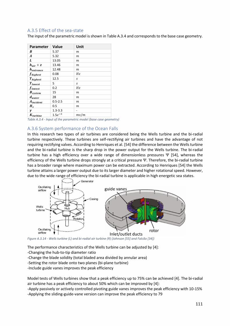
111

A.3.5 Effect of the sea-state The input of the parametric model is shown in Table A.3.4 and corresponds to the base case geometry.

Parameter Value Unit 𝑩 5.37 𝑚

𝑨 5.32 𝑚

𝑳 13.05 𝑚

𝒉𝒂𝒊𝒓 + 𝒛 13.46 𝑚

𝒉𝒆𝒏𝒕𝒓𝒂𝒏𝒄𝒆 12.48 𝑚

𝒇𝒉𝒊𝒈𝒉𝒆𝒔𝒕 0.08 𝐻𝑧

𝑻𝒉𝒊𝒈𝒉𝒆𝒔𝒕 12.5 𝑠

𝑻𝒍𝒐𝒘𝒆𝒔𝒕 5 𝑠

𝒇𝒍𝒐𝒘𝒆𝒔𝒕 0.2 𝐻𝑧

𝑩𝒔𝒚𝒔𝒕𝒆𝒎 15 𝑚

𝒅𝒘𝒂𝒕𝒆𝒓 28 𝑚

𝑨𝒊𝒏𝒄𝒊𝒅𝒆𝒏𝒕 0.5-2.5 𝑚

𝑯𝒔 0.5 𝑚

𝜸 1.3-3.3 -

𝑲𝒕𝒖𝒓𝒃𝒊𝒏𝒆 1.5𝑒−3 𝑚𝑠/𝑚

Table A.3.4 - Input of the parametric model (base case geometry)

A.3.6 System performance of the Ocean Falls In this research two types of air turbines are considered being the Wells turbine and the bi-radial turbine respectively. These turbines are self-rectifying air turbines and have the advantage of not requiring rectifying valves. According to Henriques et al. [54] the difference between the Wells turbine and the bi-radial turbine is the sharp drop in the power output for the Wells turbine. The bi-radial turbine has a high efficiency over a wide range of dimensionless pressures Ψ [54], whereas the efficiency of the Wells turbine drops strongly at a critical pressure Ψ. Therefore, the bi-radial turbine has a broader range where maximum power can be extracted. According to Henriques [54] the Wells turbine attains a larger power output due to its larger diameter and higher rotational speed. However, due to the wide range of efficiency the bi-radial turbine is applicable in high energetic sea states.

Figure A.3.14 - Wells turbine (L) and bi-radial air turbine (R) (Johnson [55] and Falcao [34])

The performance characteristics of the Wells turbine can be adjusted by [4]: -Changing the hub-to-tip diameter ratio -Change the blade solidity (total bladed area divided by annular area) -Setting the rotor blade onto two planes (bi-plane turbine) -Include guide vanes improves the peak efficiency Model tests of Wells turbines show that a peak efficiency up to 75% can be achieved [4]. The bi-radial air turbine has a peak efficiency to about 50% which can be improved by [4]: -Apply passively or actively controlled pivoting guide vanes improves the peak efficiency with 10-15% -Applying the sliding-guide-vane version can improve the peak efficiency to 79

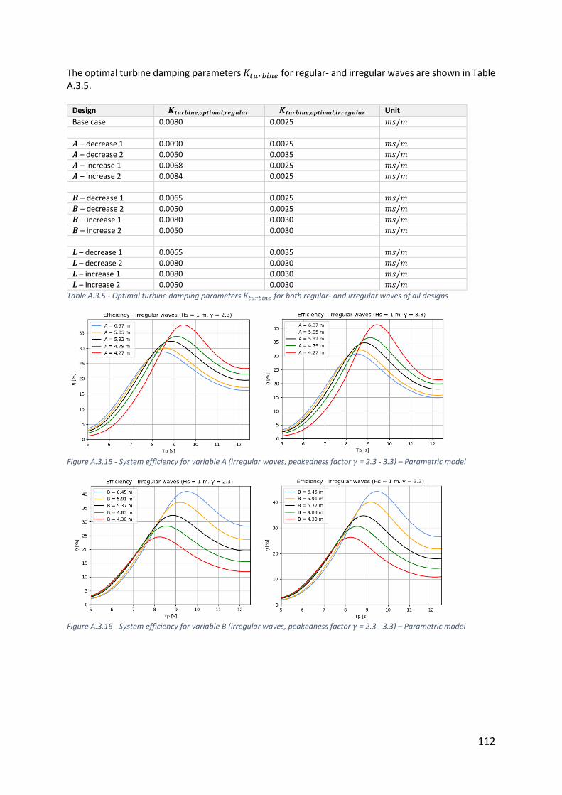
112

The optimal turbine damping parameters 𝐾𝑡𝑢𝑟𝑏𝑖𝑛𝑒 for regular- and irregular waves are shown in Table A.3.5.

Design 𝑲𝒕𝒖𝒓𝒃𝒊𝒏𝒆,𝒐𝒑𝒕𝒊𝒎𝒂𝒍,𝒓𝒆𝒈𝒖𝒍𝒂𝒓 𝑲𝒕𝒖𝒓𝒃𝒊𝒏𝒆,𝒐𝒑𝒕𝒊𝒎𝒂𝒍,𝒊𝒓𝒓𝒆𝒈𝒖𝒍𝒂𝒓 Unit

Base case 0.0080 0.0025 𝑚𝑠/𝑚

𝑨 – decrease 1 0.0090 0.0025 𝑚𝑠/𝑚

𝑨 – decrease 2 0.0050 0.0035 𝑚𝑠/𝑚

𝑨 – increase 1 0.0068 0.0025 𝑚𝑠/𝑚

𝑨 – increase 2 0.0084 0.0025 𝑚𝑠/𝑚

𝑩 – decrease 1 0.0065 0.0025 𝑚𝑠/𝑚

𝑩 – decrease 2 0.0050 0.0025 𝑚𝑠/𝑚

𝑩 – increase 1 0.0080 0.0030 𝑚𝑠/𝑚

𝑩 – increase 2 0.0050 0.0030 𝑚𝑠/𝑚

𝑳 – decrease 1 0.0065 0.0035 𝑚𝑠/𝑚

𝑳 – decrease 2 0.0080 0.0030 𝑚𝑠/𝑚

𝑳 – increase 1 0.0080 0.0030 𝑚𝑠/𝑚

𝑳 – increase 2 0.0050 0.0030 𝑚𝑠/𝑚

Table A.3.5 - Optimal turbine damping parameters 𝐾𝑡𝑢𝑟𝑏𝑖𝑛𝑒 for both regular- and irregular waves of all designs

Figure A.3.15 - System efficiency for variable A (irregular waves, peakedness factor 𝛾 = 2.3 - 3.3) – Parametric model

Figure A.3.16 - System efficiency for variable B (irregular waves, peakedness factor 𝛾 = 2.3 - 3.3) – Parametric model

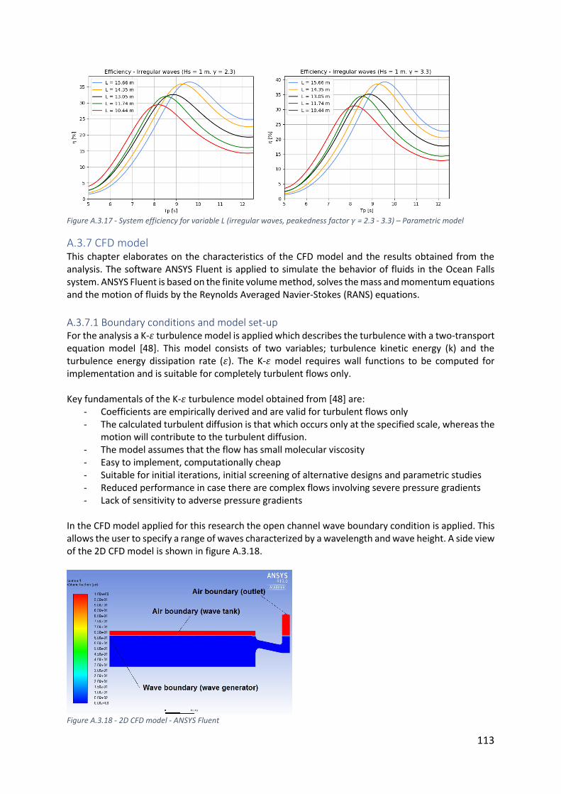
113

Figure A.3.17 - System efficiency for variable L (irregular waves, peakedness factor 𝛾 = 2.3 - 3.3) – Parametric model

A.3.7 CFD model This chapter elaborates on the characteristics of the CFD model and the results obtained from the analysis. The software ANSYS Fluent is applied to simulate the behavior of fluids in the Ocean Falls system. ANSYS Fluent is based on the finite volume method, solves the mass and momentum equations and the motion of fluids by the Reynolds Averaged Navier-Stokes (RANS) equations.

A.3.7.1 Boundary conditions and model set-up For the analysis a K-휀 turbulence model is applied which describes the turbulence with a two-transport equation model [48]. This model consists of two variables; turbulence kinetic energy (k) and the turbulence energy dissipation rate (휀). The K-휀 model requires wall functions to be computed for implementation and is suitable for completely turbulent flows only. Key fundamentals of the K-휀 turbulence model obtained from [48] are:

- Coefficients are empirically derived and are valid for turbulent flows only - The calculated turbulent diffusion is that which occurs only at the specified scale, whereas the

motion will contribute to the turbulent diffusion. - The model assumes that the flow has small molecular viscosity - Easy to implement, computationally cheap - Suitable for initial iterations, initial screening of alternative designs and parametric studies - Reduced performance in case there are complex flows involving severe pressure gradients - Lack of sensitivity to adverse pressure gradients

In the CFD model applied for this research the open channel wave boundary condition is applied. This allows the user to specify a range of waves characterized by a wavelength and wave height. A side view of the 2D CFD model is shown in figure A.3.18.

Figure A.3.18 - 2D CFD model - ANSYS Fluent

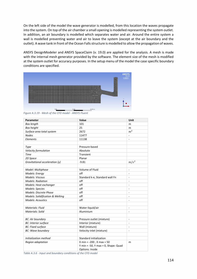
114

On the left side of the model the wave generator is modelled, from this location the waves propagate into the system. On top of the air chamber a small opening is modelled representing the system outlet. In addition, an air boundary is modelled which separates water and air. Around the entire system a wall is modelled preventing water and air to leave the system (except at the air boundary and the outlet). A wave tank in front of the Ocean Falls structure is modelled to allow the propagation of waves. ANSYS DesignModeler and ANSYS SpaceClaim (v. 19.0) are applied for the analysis. A mesh is made with the internal mesh generator provided by the software. The element size of the mesh is modified at the system outlet for accuracy purposes. In the setup menu of the model the case specific boundary conditions are specified.

Figure A.3.19 - Mesh of the CFD model - ANSYS Fluent

Parameter Value Unit

Box length 101 𝑚

Box height 25 𝑚

Surface area total system 2672 𝑚2

Nodes 11477 -

Elements 11138 -

Type Pressure-based

Velocity formulation Absolute

Time Transient

2D Space Planar

Gravitational acceleration (y) -9.81 𝑚/𝑠2

Model: Multiphase Volume of Fluid -

Models: Energy off -

Models: Viscous Standard k-e, Standard wall Fn -

Models: Radiation off -

Models: Heat exchanger off -

Models: Species off -

Models: Discrete Phase off -

Models: Solidification & Melting off -

Models: Acoustics off -

Materials: Fluid Water-liquid/air -

Materials: Solid Aluminium -

BC: Air boundary Pressure outlet (mixture) -

BC: Interior surface Interior (mixture) -

BC: Fixed surface Wall (mixture) -

BC: Wave boundary Velocity-inlet (mixture) -

Initialization method Standard initialization

Region adaptation X min = -200 , X max = 50 Y min = -50, Y max = 0, Shape: Quad Options: Inside

m

Table A.3.6 - Input and boundary conditions of the CFD model

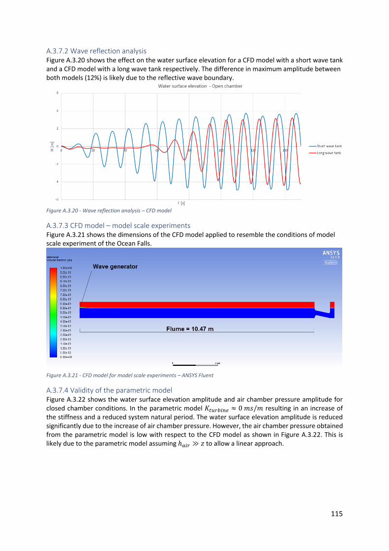
115

A.3.7.2 Wave reflection analysis Figure A.3.20 shows the effect on the water surface elevation for a CFD model with a short wave tank and a CFD model with a long wave tank respectively. The difference in maximum amplitude between both models (12%) is likely due to the reflective wave boundary.

Figure A.3.20 - Wave reflection analysis – CFD model

A.3.7.3 CFD model – model scale experiments Figure A.3.21 shows the dimensions of the CFD model applied to resemble the conditions of model scale experiment of the Ocean Falls.

Figure A.3.21 - CFD model for model scale experiments – ANSYS Fluent

A.3.7.4 Validity of the parametric model Figure A.3.22 shows the water surface elevation amplitude and air chamber pressure amplitude for closed chamber conditions. In the parametric model 𝐾𝑡𝑢𝑟𝑏𝑖𝑛𝑒 ≈ 0 𝑚𝑠/𝑚 resulting in an increase of the stiffness and a reduced system natural period. The water surface elevation amplitude is reduced significantly due to the increase of air chamber pressure. However, the air chamber pressure obtained from the parametric model is low with respect to the CFD model as shown in Figure A.3.22. This is likely due to the parametric model assuming ℎ𝑎𝑖𝑟 ≫ 𝑧 to allow a linear approach.

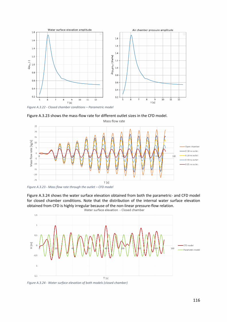
116

Figure A.3.22 - Closed chamber conditions – Parametric model

Figure A.3.23 shows the mass-flow rate for different outlet sizes in the CFD model.

Figure A.3.23 - Mass flow rate through the outlet – CFD model

Figure A.3.24 shows the water surface elevation obtained from both the parametric- and CFD model for closed chamber conditions. Note that the distribution of the internal water surface elevation obtained from CFD is highly irregular because of the non-linear pressure-flow relation.

Figure A.3.24 - Water surface elevation of both models (closed chamber)

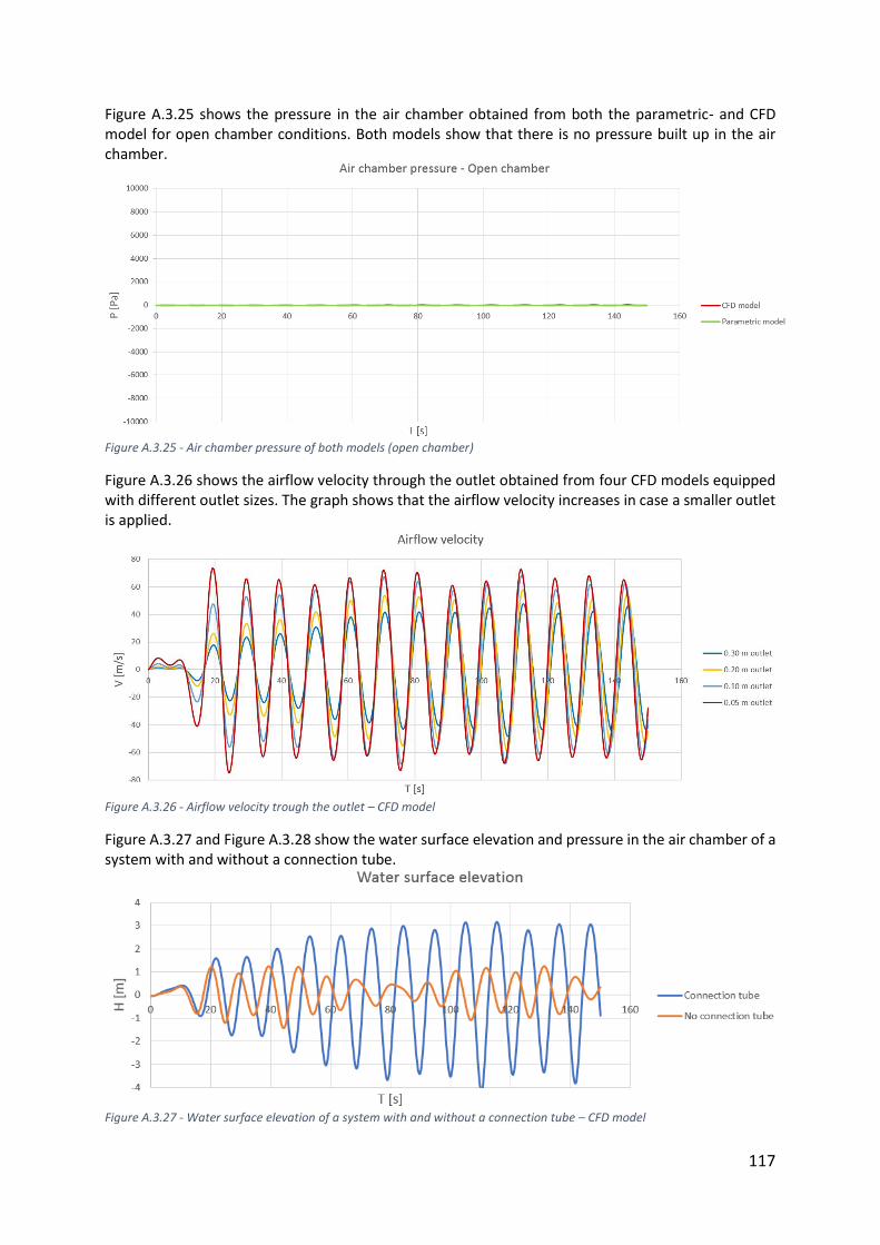
117

Figure A.3.25 shows the pressure in the air chamber obtained from both the parametric- and CFD model for open chamber conditions. Both models show that there is no pressure built up in the air chamber.

Figure A.3.25 - Air chamber pressure of both models (open chamber)

Figure A.3.26 shows the airflow velocity through the outlet obtained from four CFD models equipped with different outlet sizes. The graph shows that the airflow velocity increases in case a smaller outlet is applied.

Figure A.3.26 - Airflow velocity trough the outlet – CFD model

Figure A.3.27 and Figure A.3.28 show the water surface elevation and pressure in the air chamber of a system with and without a connection tube.

Figure A.3.27 - Water surface elevation of a system with and without a connection tube – CFD model

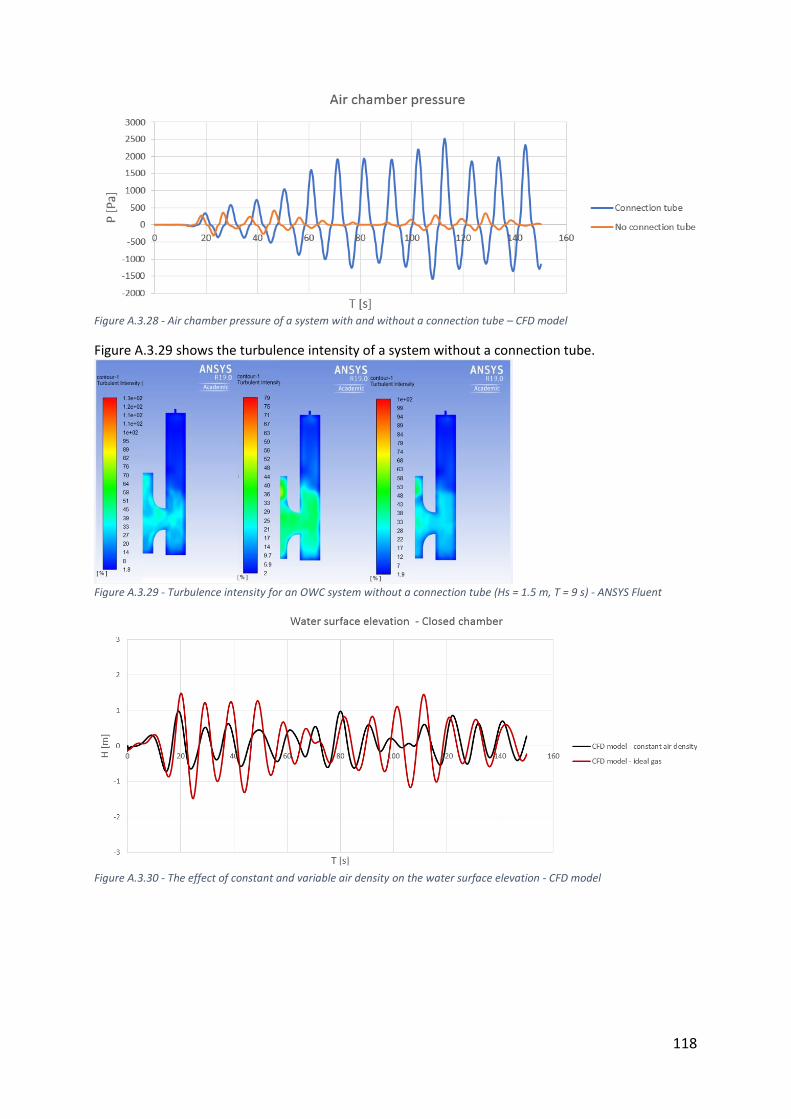
118

Figure A.3.28 - Air chamber pressure of a system with and without a connection tube – CFD model

Figure A.3.29 shows the turbulence intensity of a system without a connection tube.

Figure A.3.29 - Turbulence intensity for an OWC system without a connection tube (Hs = 1.5 m, T = 9 s) - ANSYS Fluent

Figure A.3.30 - The effect of constant and variable air density on the water surface elevation - CFD model

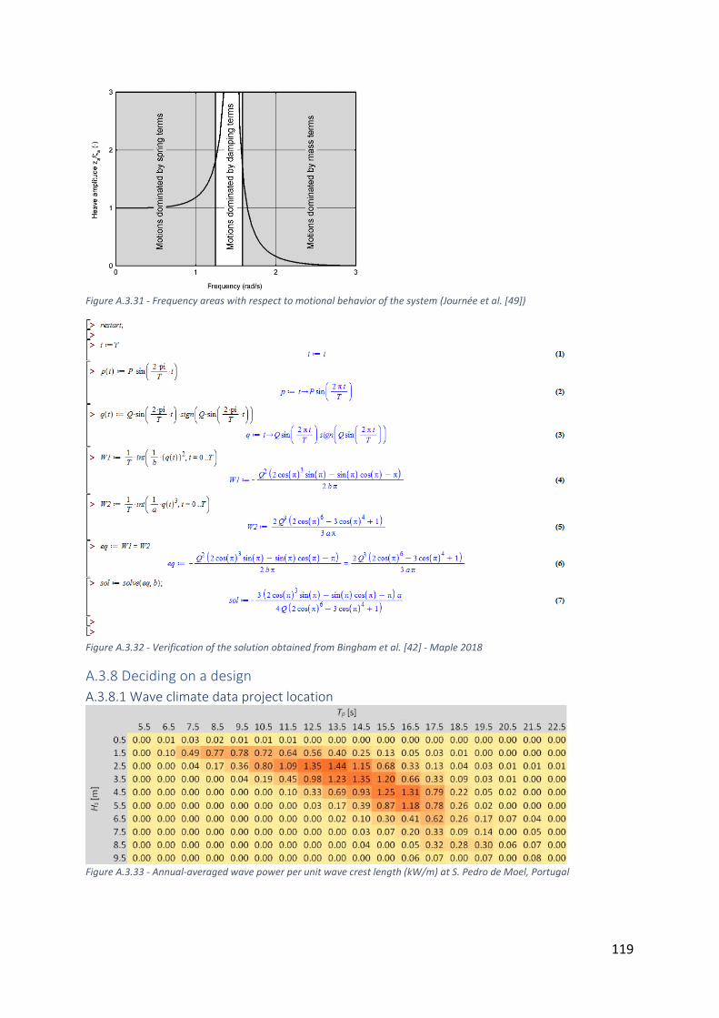
119

Figure A.3.31 - Frequency areas with respect to motional behavior of the system (Journée et al. [49])

Figure A.3.32 - Verification of the solution obtained from Bingham et al. [42] - Maple 2018

A.3.8 Deciding on a design

A.3.8.1 Wave climate data project location

Figure A.3.33 - Annual-averaged wave power per unit wave crest length (kW/m) at S. Pedro de Moel, Portugal

120

Table A.3.7 shows the fixed requirements of the dry-dock and floating dock respectively.

Value Unit

Dry-dock

Length 320 m

Width 100 m

Max draught during 2 hours 13 m

Permanent draught 10 m

Depth waterway 10 m

Floating dock

Length 200 m

Width and door opening 90 m

Max draught during 2 hours 13.5 m

Permanent draught 9 m

Depth waterway 10 m

Table A.3.7 - Concept case requirements of the dry-dock and the floating dock

A.3.8.1 Cost calculation The information of the cost calculation is shown in Table A.3.8 and is obtained from [37] and [40].

Production rate

Unit cost unit rate

Unit Quantities Costs

Foundation layer (marine placing and leveling 1m crushed stone)

200 m3/d 40 €/m3 304 m3 € 12488

Ballast material in caisson 800 m3/d 30 €/m3 80.55 m3 € 2417

Air turbine installation (incl. investment)

0.33 Units/d 60000 € 1 turbine € 60000

Floating dock:

Rent (incl. cranes and additional supplies)

90000 €/wk 1 dock - 18.12 weeks € 1630272

- Crew, energy supply etc. 20000 €/wk 18.12 weeks € 362283

Dry-dock:

- Rent (incl. cranes and add. supplies)

40000 €/wk 1 dock - 18.12 weeks € 724565

- Crew, energy supply etc. 20000 €/wk 18.12 weeks € 362283

Labour 40 €/mh 2744 mh € 109761

Concrete 120 €/m3 1519.63 m3 € 182355.64

- Concreting a slab 0.1 mh/m3 60.73 mh (608 m3)

- Concreting a wall 0.2 mh/m3 43.21 mh (216 m3)

Reinforcing steel (incl. cutting and installation)

10 mh/ton 1000 €/ton 1192.91 mh (15.19 m3) € 119290.98

Formwork (plywood) 20 €/m2 3254.98 m2 € 65100

Formwork (preparation + supports)

0.5 mh/m2 50 €/m2 3254.98 m2 € 162749

Total construction time 18.11 weeks

Total Incl. floating dock € 2718339.38

Incl. dry-dock € 1812632.99

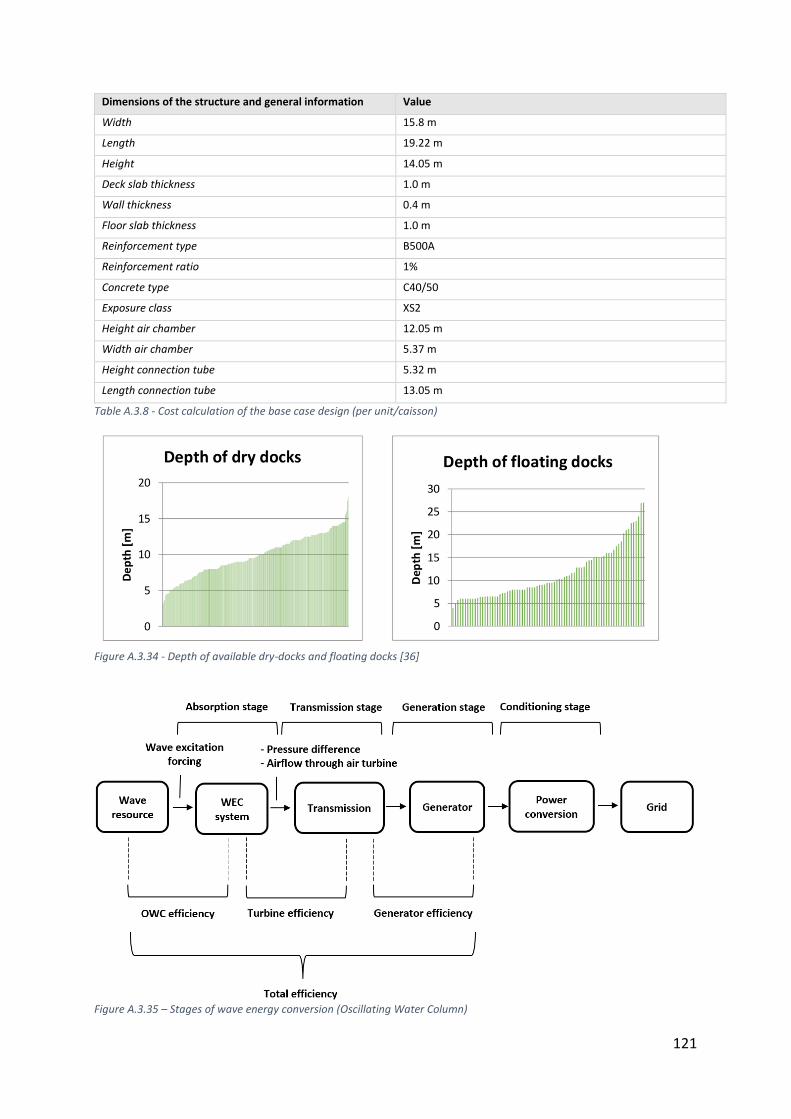
121

Dimensions of the structure and general information Value

Width 15.8 m

Length 19.22 m

Height 14.05 m

Deck slab thickness 1.0 m

Wall thickness 0.4 m

Floor slab thickness 1.0 m

Reinforcement type B500A

Reinforcement ratio 1%

Concrete type C40/50

Exposure class XS2

Height air chamber 12.05 m

Width air chamber 5.37 m

Height connection tube 5.32 m

Length connection tube 13.05 m

Table A.3.8 - Cost calculation of the base case design (per unit/caisson)

Figure A.3.34 - Depth of available dry-docks and floating docks [36]

Figure A.3.35 – Stages of wave energy conversion (Oscillating Water Column)

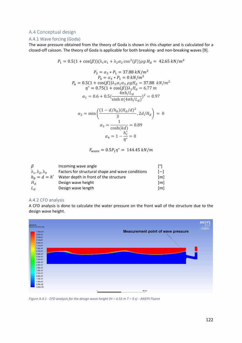
122

A.4 Conceptual design

A.4.1 Wave forcing (Goda) The wave pressure obtained from the theory of Goda is shown in this chapter and is calculated for a closed-off caisson. The theory of Goda is applicable for both breaking- and non-breaking waves [9].

𝑃1 = 0.5(1 + cos(𝛽))(λ1𝛼1 + λ2𝛼2 cos2(𝛽))𝜌𝑔 𝐻𝑑 = 42.65 𝑘𝑁/𝑚2

𝑃3 = 𝛼3 ∗ 𝑃1 = 37.88 𝑘𝑁/𝑚2 𝑃4 = 𝛼4 ∗ 𝑃1 = 0 𝑘𝑁/𝑚2

𝑃𝑢 = 0.5(1 + cos(𝛽))λ3𝛼1𝛼3 𝜌𝑔𝐻𝑑 = 37.88 𝑘𝑁/𝑚2 휂∗ = 0.75(1 + cos(𝛽))λ1𝐻𝑑 = 6.77 𝑚

𝛼1 = 0.6 + 0.5(4𝜋ℎ/𝐿𝑑

sinh 𝜋(4𝜋ℎ/𝐿𝑑))2 = 0.97

𝛼2 = min ((1 − 𝑑/ℎ𝑏)(𝐻𝑑/𝑑)2

3, 2𝑑/𝐻𝑑) = 0

𝛼3 =1

cosh (𝑘𝑑)= 0.89

𝛼4 = 1 −ℎ𝑐

∗

휂∗= 0

𝐹𝑤𝑎𝑣𝑒 = 0.5𝑃1휂∗ = 144.45 𝑘𝑁/𝑚

𝛽 Incoming wave angle [°] λ1, λ2, λ3 Factors for structural shape and wave conditions [−] ℎ𝑏 = 𝑑 = ℎ′ Water depth in front of the structure [𝑚] 𝐻𝑑 Design wave height [𝑚] 𝐿𝑑 Design wave length [𝑚]

A.4.2 CFD analysis A CFD analysis is done to calculate the water pressure on the front wall of the structure due to the design wave height.

Figure A.4.1 - CFD analysis for the design wave height (H = 4.55 m T = 9 s) - ANSYS Fluent

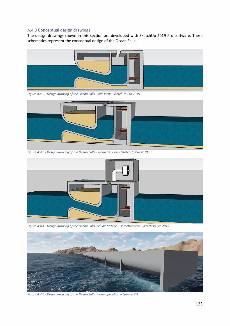
123

A.4.3 Conceptual design drawings The design drawings shown in this section are developed with SketchUp 2019 Pro software. These schematics represent the conceptual design of the Ocean Falls.

Figure A.4.2 - Design drawing of the Ocean Falls - Side view - SketchUp Pro 2019

Figure A.4.3 - Design drawing of the Ocean Falls – Isometric view - SketchUp Pro 2019

Figure A.4.4 - Design drawing of the Ocean Falls incl. air turbine - Isometric view - SketchUp Pro 2019

Figure A.4.5 - Design drawing of the Ocean Falls during operation – Lumion 3D

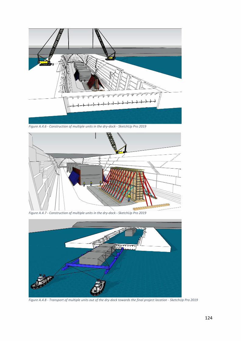
124

Figure A.4.6 - Construction of multiple units in the dry-dock - SketchUp Pro 2019

Figure A.4.7 - Construction of multiple units in the dry-dock - SketchUp Pro 2019

Figure A.4.8 - Transport of multiple units out of the dry-dock towards the final project location - SketchUp Pro 2019

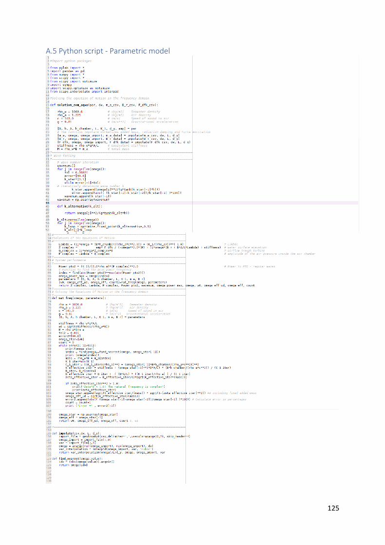
125

A.5 Python script - Parametric model

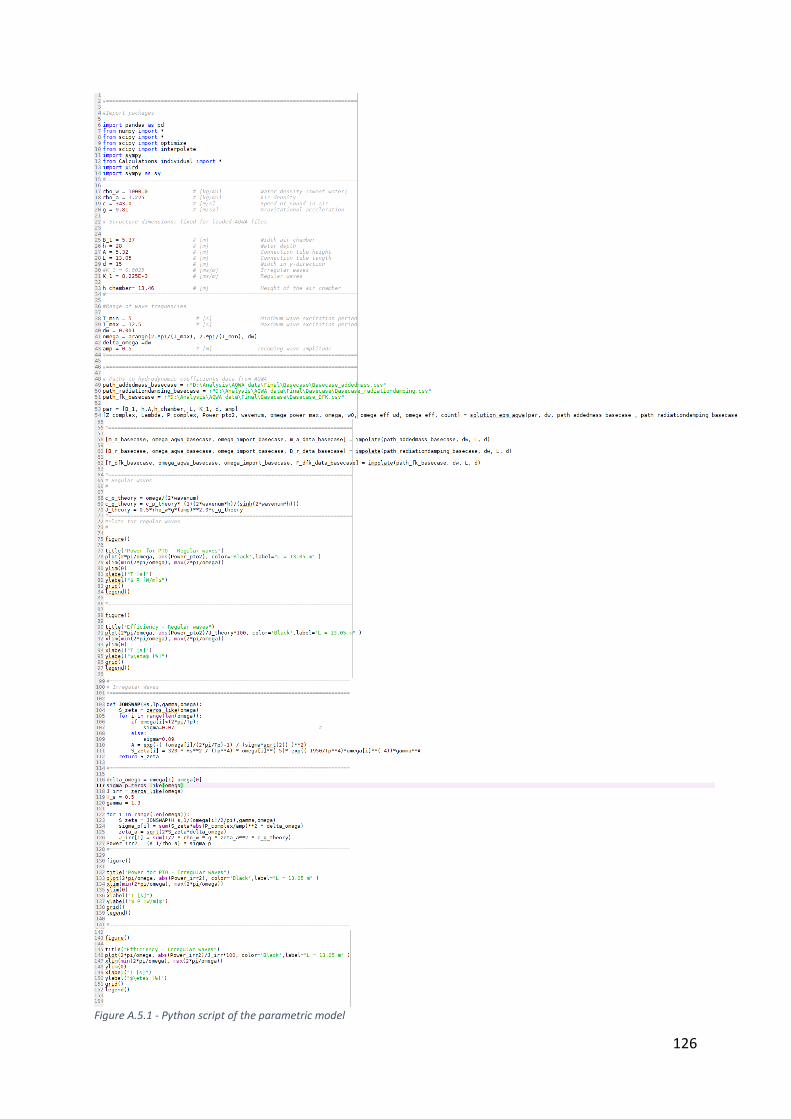
126

Figure A.5.1 - Python script of the parametric model

Faculty of Civil Engineering and Geosciences Stevinweg 1 2628 CN Delft The Netherlands