Percolation on correlated random networks

APS/123-QED

Percolation on correlated random networks

E. Agliari,1, 2, 3 C. Cioli,4 and E. Guadagnini5, 6

1Dipartimento di Fisica, Universita degli Studi di Parma, Italy2INFN, Sezione di Parma

3Theoretische Polymerphysik, Albert-Ludwig-Universitat, Freiburg, Germany4Center for Complexity Science, University of Warwick, United Kingdom

5Dipartimento di Fisica, Universita di Pisa, Italy6INFN, Sezione di Pisa

(Dated: September 6, 2011)

We consider a class of random, weighted networks, obtained through a redefinition of patterns in anHopfield-like model and, by performing percolation processes, we get information about topology andresilience properties of the networks themselves. Given the weighted nature of the graphs, differentkinds of bond percolation can be studied: stochastic (deleting links randomly) and deterministic(deleting links based on rank weights), each mimicking a different physical process. The evolutionof the network is accordingly different, as evidenced by the behavior of the largest component sizeand of the distribution of cluster sizes. In particular, we can derive that weak ties are crucial inorder to maintain the graph connected and that, when they are the most prone to failure, thegiant component typically shrinks without abruptly breaking apart; these results have been recentlyevidenced in several kinds of social networks.

PACS numbers: 89.75.Fb.+q,05.70.Fh,64.60.ah, 82.20.Wt

I. INTRODUCTION

Network theory is a fundamental tool for the modernunderstanding of complex systems: by a simple graphrepresentation, where the elementary units of a sys-tem become nodes and their mutual interactions becomelinks, a lot of properties about the structure and dynam-ics of the system itself can be inferred [1].

Recently, the characterization of network dynamics hasbecome a central issue: networks are intrinsically dy-namic and continuously accommodate novel members,lose their original elements, as well as build, erase andrearrange their links [2]. The structural reorganizationof networks may arise due, e.g., to a change in the re-sources providing the energy to maintain their links, orto a large stress [3, 4]. In this context, percolation [5, 6]constitutes a very interesting process able to mimic a fail-ure or a damage of links/nodes. Moreover, percolationrepresents one of the simplest example of dynamical pro-cess on a graph, exhibiting a phase transitions [7] and,indeed, it has been mapped into several other criticalphenomena; as well, applications in epidemiology, traf-fic models and in the analysis of technological networksresilience have been deeply studied [8–11].

Here we apply percolation processes as a means in or-der to probe the topology and the resilience of a net-work itself. We especially focus on a class of stochas-tic, weighted networks G recently introduced in [12, 13].Such networks are generated by assigning to each node aset of attributes and by linking two nodes whenever thepertaining attributes are similar enough; the larger thesimilarity, the stronger the link. As shown in [12, 13], theresulting class of (weighted) networks G exhibits interest-ing properties such as imitative interactions (by construc-tion), degree-degree correlation, high transitivity (i.e. a

large clustering coefficient) and a properly tunable topol-ogy through a parameter θ, which controls the distribu-tion of attributes. Therefore, such networks constitutean efficient tool to describe several different systems thatbelong to disparate contexts, ranging from biological net-works [14, 15], to technological structures [16] and to so-cial organizations [17–19].

Now, since the graphs under investigation areweighted, we can perform different kinds of percola-tion processes: random (where links are deleted in apurely random fashion), and deterministic (where linksare deleted in rank order from the weakest to strongest, orvice versa). We especially focus on graphs G obtained forθ = 0 and θ = 0.25, corresponding (in the limit of largesize) to fully connected weighted networks and account-ing for an “unbiased” and “biased” pattern distribution,respectively. First of all, we consider the relative size ofthe largest connected component S as a function of thefraction f of links left: numerical data suggest that a “gi-ant component” emerges when the fraction f approachesa “critical” value fc, which is found to scale with thesystem size according to V −ν , where ν depends on thekind of dilution. The latter also controls the sharpnessof the percolation, as well as the distribution of clustersizes, showing that, for biased pattern distributions, weakties play a crucial role as they can be used to build upa spanning tree, conversely, strongest links are typicallyredundant, as a result, if weak ties are the most prone tofailure the system will exhibit a poor resilience.

The paper is organized as follows: in Sec. II we describethe correlated random networks we are focusing on, aswell as the percolation processes we perform. Then, inSec. III we present the basic probability relations con-cerning the coupling distribution, from which we can in-fer qualitative information on the properties of the per-

arX

iv:1

109.

0839

v1 [

cond

-mat

.sta

t-m

ech]

5 S

ep 2

011

2

colation transition; these properties are confirmed by theresults of the numerical analysis that is reported in thefollowing sections. In particular, the behavior of the gi-ant component is studied in Sec. IV, the distribution ofcluster sizes is described in Sec. V and the behavior of theclustering coefficient is examined in Sec. VI. An overalldiscussion on the results and on the perspectives of ourwork is contained in Sec. VII. In Appendix A we showthat the class of graphs that we consider displays dissor-tative mixing in a wide region of the parameter set, whilein Appendix B we present some analytic results which arevalid for the random percolation process on G.

II. THE MODEL

We first introduce the class of networks on which wefocus our analysis and later we describe the percolativeprocesses we will perform on such networks.

A. Network generation

Recently, a new approach to generate correlated ran-dom networks has been introduced [12, 13]; the approachis based on a simple shift [−1,+1] → [0,+1] in the defi-nition of patterns in an Hopfield-like model and it allowsto generate a broad variety of different topologies rang-ing from fully-connected to small-world, to extremely di-luted.

More precisely, we consider a set of V nodes, eachendowed with a set of L attributes encoded by a bi-nary string ξ; the ensemble of strings is extracted ac-cording to the probabilities P (ξµ = 0) = (1 − a)/2 andP (ξµ = 1) = (1 + a)/2, where the fixed parameter a be-longs to the interval [−1, 1]. Then, the coupling betweentwo generic nodes i and j is given by the rule

Jij =

L∑µ=1

ξµi ξµj . (1)

Therefore, the wider the overlap between non-null en-tries and the larger the weight associated to the link,with Jij ∈ [0, L]; the extreme case Jij = 0 means thatthere exists no link between nodes i and j. The valuestaken by the strings components admit the following in-terpretation: ξµi = 1 means that agent i is endowed withthe particular feature µ, this feature can represent a bi-ological trait or an individual attitude according to theconsidered system (the absence of this particular featurecorresponds to ξµi = 0). Then Eq. 1 states that agentsshow homophily. For example, in social networks, peopleinteract with others of similar age, income, race, etc.

As shown in [12, 13], the way a node is connected tothe network is sensitively affected by the number ρ ofnon-null entries present in the pertaining string, that is,for the i-th node, ρi =

∑µ ξ

µi (notice that since ρ is

Poissonian, its average is given by ρ = L(1 + a)/2). In

fact, one finds that the average probability Plink(ρi; a)that i is connected to another generic node, reads as

Plink(ρi; a) = 1−(

1− a2

)ρi.

Moreover, by averaging over all possible string arrange-ments, one finds for the average link probability p be-tween two generic nodes

p = 1−

[1−

(1 + a

2

)2]L

.

The class of networks that are generated in this wayexhibit different levels of correlation. For instance, it iseasy to see [12, 13] that two neighbors of a given nodeare more likely to be connected than they would be if thegraph was purely random generated; this kind of transi-tivity also affects the weights associated with the links[12, 13]. Such networks also display a dissortative be-havior. Indeed, the nodes having strings with small ρtypically possess a small coordination number and theyare more likely to be linked with nodes with large ρ. Themathematical aspects of the degree correlations are elab-orated in Appendix A.

Finally, we introduce the parameter α = L/V whichturns out to crucially control not only the topology butalso the thermodynamic of the system [12, 13]. Here weassume α to be constant and finite, which means that,as the volume of the system grows, the length of thestring increases proportionally; this corresponds the theso-called high-storage regime in neural networks [20]. In-terestingly, as V → ∞ there exists a vanishingly smallrange of values for a giving rise to a non-trivial graph;such a range can be recognized by the following scaling

a = −1 +γ

V θ, (2)

where θ ≥ 0 and γ is a finite parameter. As explained in[13], θ controls the connectivity regime of the network-ranging from fully connected (FC, 0 ≤ θ < 1/2) to ex-tremely diluted (1/2 < θ < 1) to completely disconnected(θ > 1), while γ allows a fine tuning. In particular, herewe focus on θ < 1/2 and γ < 2, corresponding to a FCregime: in this case topological disorder is lost, while dis-order on couplings is still present; however, notice thatfor θ = 0 and γ = 2, the coupling distribution gets peakedat J = L and disorder on couplings is relaxed as well.

In the following, we will refer to the weighted randomgraph, generated as explained above, as G(α, θ, γ, L),hence highlighting the dependence on the set of param-eters which control its size and its topology. We alsoanticipate that we will focus only on the cases θ = 0 andθ = 0.25 corresponding to weighted, complete graphs. Ofcourse, for these cases there is no topological correlationamong links (the clustering coefficient is equal to 1 andassortativity is neutral), though correlation among linkcouplings is retained.

3

B. Percolation processes

Given an arbitrary graph, bond percolation consists indeleting the existing links with some probability 1 − for, in other terms, in occupying links with probabilityf ; nodes connected together form clusters. When f ex-ceeds a given system-dependent threshold (or critical)value fc, a macroscopic cluster, i.e. a cluster occupying afinite fraction of all available sites, also called giant com-ponent, is formed. For various network architectures andspace dimensionalities this transition is typically contin-uous, or second-order, as the system properties changescontinuously at the critical point [5, 21]. For instance, onrandom networks a la Erdos-Renyi (ER) [22], one startsfrom a set of V nodes and adds links such that the prob-ability f that two nodes are joined by a link is the samefor all pairs of nodes. When f < 1/V , the largest com-ponent remains miniscule, its number of vertices scalingas log V ; in contrast, if f > 1/V , there is a componentof size linear in V . Thus, the fraction of vertices in thelargest component undergoes a continuous phase transi-tion at f = 1/V .

As explained before, in the graph under studyquenched weights are assigned to the edges and this al-lows to think of different kinds of processes, each cor-responding to different physical situations: The deletionof a link may mimic the failure of the link itself due tooverload [4] or, rather, to error or attack which may af-fect randomly any link [23]. In the former case linkswith higher weight are the first to be deleted, while inthe latter case deletion occurs randomly. In other kindsof situations we can think that nodes transfer a signal toneighbors and the passage of information is effective onlywhen the tie strength is larger than some noise level [24].Therefore, as the level of noise grows, more and morelinks starting from the weakest ones, get ineffective. Tosummarize, we deal with the following processes:

• Random percolation (RP): starting from the origi-nal graph G(α, θ, γ, L) we consider each link and weremove it with probability 1 − f , independently ofthe couple of adjacent nodes, in such a way that fis the fraction of links left; as f is tuned from 0 to1 we range from a completely disconnected graphto the original graph.

• Deterministic-Weak percolation (WP): startingfrom G(α, θ, γ, L), we remove all links with weightsmaller than a given threshold ι; that is to say, as ιis tuned from 0 to L, we remove links in rank orderfrom the weakest to strongest ties.

• Deterministic-Strong percolation (SP): startingfrom G(α, θ, γ, L), we remove all links with weightlarger than a given threshold ι; analogously to theprevious case, this corresponds to remove links inrank order from the strongest to the weakest ties.

In order to evaluate the impact of removing ties, wemeasure the relative size of the largest connected compo-

nent S, providing the fraction of nodes that can all reacheach other through connected paths, as a function of thefraction f of links left f . We also measure the average

squared size S =∑Vs=1 nss

2/V , where ns is the numberof clusters containing s nodes. According to percolationtheory, if the (infinite) network collapses because of aphase transition at fc, then S diverges as f approachesf−c [5, 25].

III. COUPLING DISTRIBUTION

The coupling distribution Pcoupl(J ; a, L) plays an im-portant role as for deterministic processes, so that it isworth recalling some previous results [12] and deepeningits dependence on the system parameters.

The probability for two strings ξi and ξj (with ρi and ρjnon-null entries) to be connected by a link with weight Jis just the probability that the strings display J effectivematchings; this has been found to be [12]

Pmatch(J ; ρi, ρj , L) =

(LJ

)(L−Jρi−J

)(L−ρiρj−J

)(Lρi

)(Lρj

) , (3)

from which we can write that, in the average, the cou-pling distribution reads off as

Pcoupl(J ; a, L) =

L∑ρi=0

L∑ρj=0

Pmatch(J ; ρi, ρj , L)

× P1(ρi; a, L)P1(ρj ; a, L), (4)

being P1(ρ; a, L) =(Lρ

)[(1+a)/2]ρ[(1−a)/2]L−ρ the prob-

ability that a given string displays ρ non-null entries.Therefore, we get

Pcoupl(J ; a, L) =

(L

J

)(a+ 1)−2L (5)

×L∑

ρi=0

L∑ρj=0

(L− Jρi − J

)(L− ρiρ2 − J

)aρi+ρj ,

where we called a = (1+a)/(1−a). Since we are focusingon the case L = αV , with a string bias a given by Eq. 2,it is convenient to rewrite the coupling distribution as afunction of the effective parameters, namely

Pcoupl(J ;α, θ, γ, L) =

(L

J

)[1− γ

2(L/α)θ

]2L× (6)

L∑ρi=0

L∑ρj=0

(L− Jρi − J

)(L− ρiρj − J

)[γ

2(L/α)θ − γ

]ρi+ρj.

The previous expression shows that for systems largeenough, and α and L fixed, the distribution gets peakedat smaller J as θ is increased (when θ > 0.5 only cou-plings with value 0 or 1 display non vanishing proba-bility) and the same holds for fluctuations. Moreover,

4

0 20 40 600

0.05

0.1

0.15

0.2

0.25

0.3

J

Pcoupl(J

;!,"

,#,L

)

0 50

0.1

0.2

0.3

0.4

0.5

0.6

0.7

0.8

J

L = 10

L = 30

L = 60

L = 100

L = 170

" = 0 " = 0.25

FIG. 1: (Color on line) Coupling distributionsPcoupl(J ;α, θ, γ, L) from different values of L (depictedin different colors, as shown by the legend) and for γ = 1,α = 0.1, θ = 0 (left panel) or θ = 0.25 (right panel). Curvesrepresent Eq. 6.

a link is absent with probability Pcoupl(0;α, θ, γ, L) =[1− γ2/4(α/L)2θ]L, which decays to zero for θ < 0.5.

In particular, in the following analysis we assume γ =1, α = 0.1 and θ = 0 or θ = 0.25; for θ = 0 we can writeexplicitly

Pcoupl(J ; 0.1, 0, 1, L) =L!

J !2−2L

L∑ρi=0

L∑ρj=0

1

(ρi − J)!(ρj − J)!(L− ρi − ρj + J)!, (7)

and similarly for the latter. In Fig. 1 we show a compari-son of the two cases where numerical data are fitted withcurves given by Eq. 6. Data corroborate that, even atrelatively small sizes, the analytical formula above pro-vide a good approximation and that the distribution getsbroader for larger L and smaller θ. More precisely, wecalculate the average coupling J(α, θ, γ, L) and its fluc-tuations ∆J((α, θ, γ, L)) as

J(α, θ, γ, L) =

L∑J=0

JPcoupl(J ;α, θ, γ, L) =γ2

4

L

(L/α)2θ,(8)

∆J(α, θ, γ, L) =

L∑J=0

(J − J)2Pcoupl(J ;α, θ, γ, L),(9)

where for the closed form expression in Eq. 8 we usedEq. 6. Relevant results are shown in Fig. 2, where, again,the comparison between analytical estimates and numer-ical data is successful.

Interestingly, from the width of the distribution onecan infer information about the sharpness of the deter-ministic percolation: a broader distribution is expected

101 102

100

101

102

L

J(!

,",#

,L)

" = 0

" = 0.25

101 10210−1

100

101

L

!J

(!

,",#

,L

)

FIG. 2: (Color on line) Log-log scale plot of the aver-age coupling J(α, θ, γ, L) (main figure) and its fluctuations∆J(α, θ, γ, L) (inset), for θ = 0 (©) and θ = 0.25 (�), asshown in the legend. Symbols represent numerical data, whilecurves represent analytical estimates from Eq. 8 and Eq. 9,respectively.

to give rise to a less sharp transition. Moreover, we no-tice that the case γ = 1 and θ = 0 corresponds to a = 0,namely it corresponds to an unbiased distribution forstrings, and this yields to a rather symmetric couplingdistribution: as a consequence, SP and WP are expectedto behave similarly. Conversely, when the coupling dis-tribution is not symmetric, as for θ = 0.25, different be-haviors emerge. All these points are deepened in the nextsection.

Finally, we notice that for θ = 0.25 relatively smallsizes give rise to non-fully-connected structures, that is,the coupling probability is non-null for J = 0. As wederived from Eq. 6, the probability that a link is absentdecreases slowly with the size and such finite-size effectgets negligible only for V ∼ 105. Indeed, we find thatfinite-size effects enhance the skewness positivity of thedistribution.

IV. PERCOLATION TRANSITIONS

In the following analysis we generate the graphG(α, θ, γ, L) and, while performing a dilution process (ei-ther deterministic or random), we measure the numberof clusters and their size; such results are then averagedover 102 realizations of G(α, θ, γ, L) in order to accountfor the stochasticity of the graph itself. As explainedin the previous section, in the thermodynamic limit bothθ = 0 and θ = 0.25 give rise to fully connected structures,so that, for large enough sizes, the random percolationprocess recovers the well-known results holding for ERgraphs [26].

In order to evaluate the impact of removing ties, wemeasure the relative size of the largest connected compo-nent S as a function of the fraction of links left f . Results

5

obtained for θ = 0 and θ = 0.25 are shown in Fig. 3 andFig. 4, respectively.

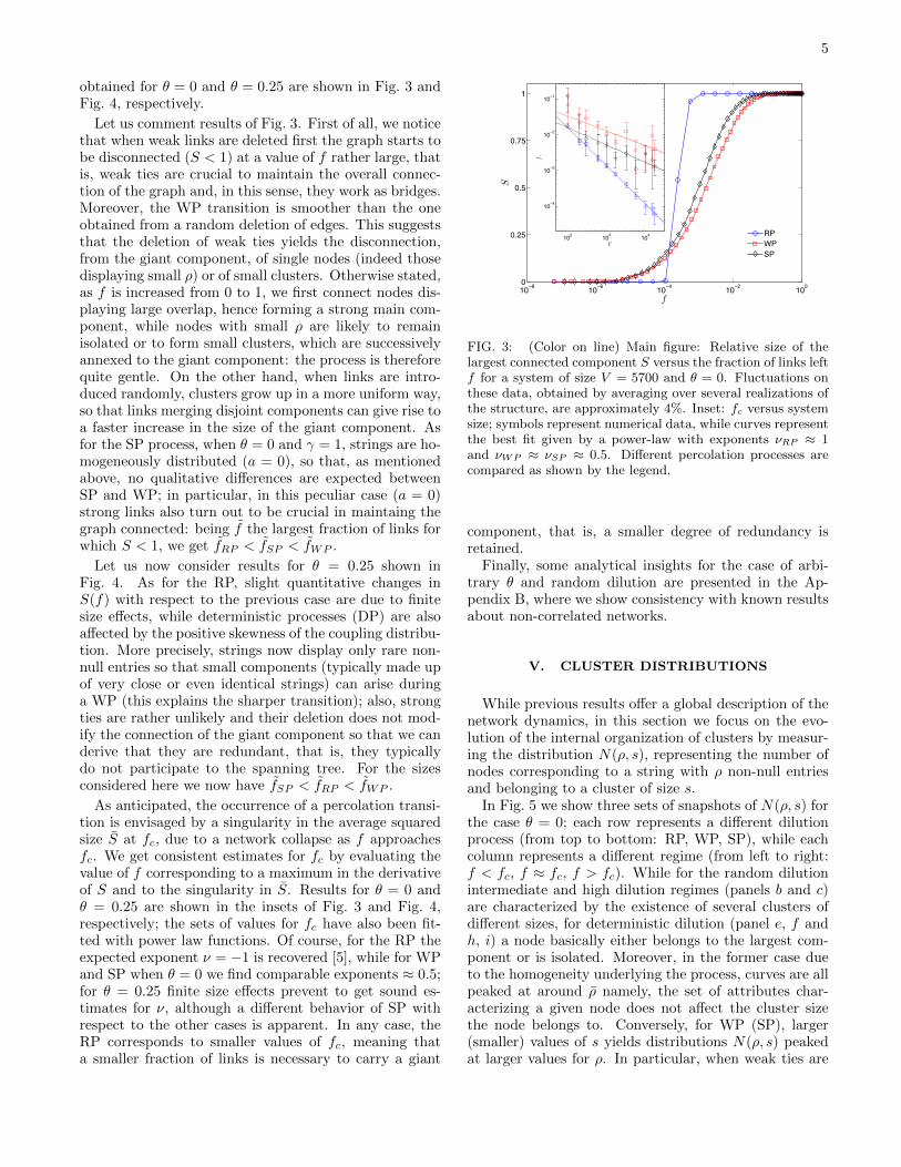
Let us comment results of Fig. 3. First of all, we noticethat when weak links are deleted first the graph starts tobe disconnected (S < 1) at a value of f rather large, thatis, weak ties are crucial to maintain the overall connec-tion of the graph and, in this sense, they work as bridges.Moreover, the WP transition is smoother than the oneobtained from a random deletion of edges. This suggeststhat the deletion of weak ties yields the disconnection,from the giant component, of single nodes (indeed thosedisplaying small ρ) or of small clusters. Otherwise stated,as f is increased from 0 to 1, we first connect nodes dis-playing large overlap, hence forming a strong main com-ponent, while nodes with small ρ are likely to remainisolated or to form small clusters, which are successivelyannexed to the giant component: the process is thereforequite gentle. On the other hand, when links are intro-duced randomly, clusters grow up in a more uniform way,so that links merging disjoint components can give rise toa faster increase in the size of the giant component. Asfor the SP process, when θ = 0 and γ = 1, strings are ho-mogeneously distributed (a = 0), so that, as mentionedabove, no qualitative differences are expected betweenSP and WP; in particular, in this peculiar case (a = 0)strong links also turn out to be crucial in maintaing thegraph connected: being f the largest fraction of links forwhich S < 1, we get fRP < fSP < fWP .

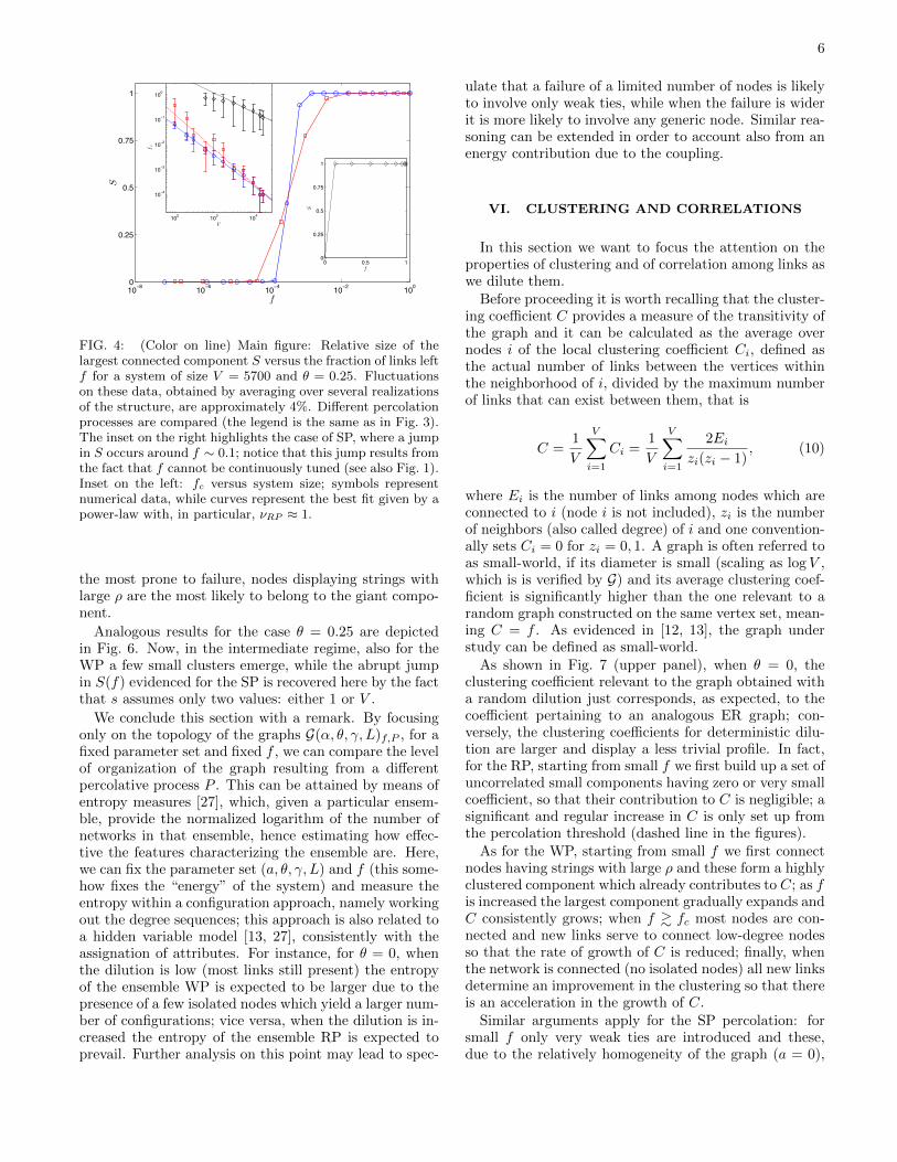
Let us now consider results for θ = 0.25 shown inFig. 4. As for the RP, slight quantitative changes inS(f) with respect to the previous case are due to finitesize effects, while deterministic processes (DP) are alsoaffected by the positive skewness of the coupling distribu-tion. More precisely, strings now display only rare non-null entries so that small components (typically made upof very close or even identical strings) can arise duringa WP (this explains the sharper transition); also, strongties are rather unlikely and their deletion does not mod-ify the connection of the giant component so that we canderive that they are redundant, that is, they typicallydo not participate to the spanning tree. For the sizesconsidered here we now have fSP < fRP < fWP .

As anticipated, the occurrence of a percolation transi-tion is envisaged by a singularity in the average squaredsize S at fc, due to a network collapse as f approachesfc. We get consistent estimates for fc by evaluating thevalue of f corresponding to a maximum in the derivativeof S and to the singularity in S. Results for θ = 0 andθ = 0.25 are shown in the insets of Fig. 3 and Fig. 4,respectively; the sets of values for fc have also been fit-ted with power law functions. Of course, for the RP theexpected exponent ν = −1 is recovered [5], while for WPand SP when θ = 0 we find comparable exponents ≈ 0.5;for θ = 0.25 finite size effects prevent to get sound es-timates for ν, although a different behavior of SP withrespect to the other cases is apparent. In any case, theRP corresponds to smaller values of fc, meaning thata smaller fraction of links is necessary to carry a giant

10 8 10 6 10 4 10 2 1000

0.25

0.5

0.75

1

f

S

RPWPSP

102 103 104

10 4

10 3

10 2

10 1

V

fc

FIG. 3: (Color on line) Main figure: Relative size of thelargest connected component S versus the fraction of links leftf for a system of size V = 5700 and θ = 0. Fluctuations onthese data, obtained by averaging over several realizations ofthe structure, are approximately 4%. Inset: fc versus systemsize; symbols represent numerical data, while curves representthe best fit given by a power-law with exponents νRP ≈ 1and νWP ≈ νSP ≈ 0.5. Different percolation processes arecompared as shown by the legend.

component, that is, a smaller degree of redundancy isretained.

Finally, some analytical insights for the case of arbi-trary θ and random dilution are presented in the Ap-pendix B, where we show consistency with known resultsabout non-correlated networks.

V. CLUSTER DISTRIBUTIONS

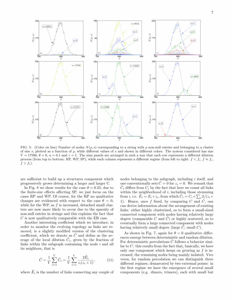
While previous results offer a global description of thenetwork dynamics, in this section we focus on the evo-lution of the internal organization of clusters by measur-ing the distribution N(ρ, s), representing the number ofnodes corresponding to a string with ρ non-null entriesand belonging to a cluster of size s.

In Fig. 5 we show three sets of snapshots of N(ρ, s) forthe case θ = 0; each row represents a different dilutionprocess (from top to bottom: RP, WP, SP), while eachcolumn represents a different regime (from left to right:f < fc, f ≈ fc, f > fc). While for the random dilutionintermediate and high dilution regimes (panels b and c)are characterized by the existence of several clusters ofdifferent sizes, for deterministic dilution (panel e, f andh, i) a node basically either belongs to the largest com-ponent or is isolated. Moreover, in the former case dueto the homogeneity underlying the process, curves are allpeaked at around ρ namely, the set of attributes char-acterizing a given node does not affect the cluster sizethe node belongs to. Conversely, for WP (SP), larger(smaller) values of s yields distributions N(ρ, s) peakedat larger values for ρ. In particular, when weak ties are

6

10 8 10 6 10 4 10 2 1000

0.25

0.5

0.75

1

f

S

102 103 104

10 4

10 3

10 2

10 1

100

V

fc

0 0.5 10

0.25

0.5

0.75

1

f

S

FIG. 4: (Color on line) Main figure: Relative size of thelargest connected component S versus the fraction of links leftf for a system of size V = 5700 and θ = 0.25. Fluctuationson these data, obtained by averaging over several realizationsof the structure, are approximately 4%. Different percolationprocesses are compared (the legend is the same as in Fig. 3).The inset on the right highlights the case of SP, where a jumpin S occurs around f ∼ 0.1; notice that this jump results fromthe fact that f cannot be continuously tuned (see also Fig. 1).Inset on the left: fc versus system size; symbols representnumerical data, while curves represent the best fit given by apower-law with, in particular, νRP ≈ 1.

the most prone to failure, nodes displaying strings withlarge ρ are the most likely to belong to the giant compo-nent.

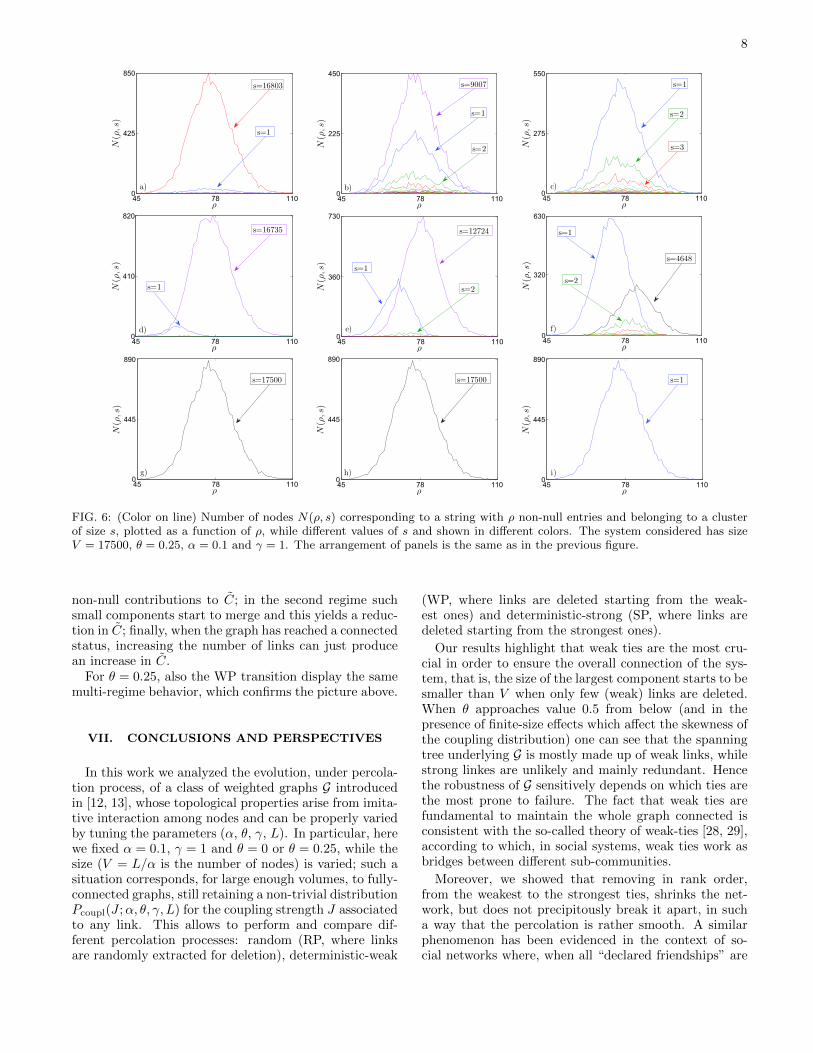
Analogous results for the case θ = 0.25 are depictedin Fig. 6. Now, in the intermediate regime, also for theWP a few small clusters emerge, while the abrupt jumpin S(f) evidenced for the SP is recovered here by the factthat s assumes only two values: either 1 or V .

We conclude this section with a remark. By focusingonly on the topology of the graphs G(α, θ, γ, L)f,P , for afixed parameter set and fixed f , we can compare the levelof organization of the graph resulting from a differentpercolative process P . This can be attained by means ofentropy measures [27], which, given a particular ensem-ble, provide the normalized logarithm of the number ofnetworks in that ensemble, hence estimating how effec-tive the features characterizing the ensemble are. Here,we can fix the parameter set (a, θ, γ, L) and f (this some-how fixes the “energy” of the system) and measure theentropy within a configuration approach, namely workingout the degree sequences; this approach is also related toa hidden variable model [13, 27], consistently with theassignation of attributes. For instance, for θ = 0, whenthe dilution is low (most links still present) the entropyof the ensemble WP is expected to be larger due to thepresence of a few isolated nodes which yield a larger num-ber of configurations; vice versa, when the dilution is in-creased the entropy of the ensemble RP is expected toprevail. Further analysis on this point may lead to spec-

ulate that a failure of a limited number of nodes is likelyto involve only weak ties, while when the failure is widerit is more likely to involve any generic node. Similar rea-soning can be extended in order to account also from anenergy contribution due to the coupling.

VI. CLUSTERING AND CORRELATIONS

In this section we want to focus the attention on theproperties of clustering and of correlation among links aswe dilute them.

Before proceeding it is worth recalling that the cluster-ing coefficient C provides a measure of the transitivity ofthe graph and it can be calculated as the average overnodes i of the local clustering coefficient Ci, defined asthe actual number of links between the vertices withinthe neighborhood of i, divided by the maximum numberof links that can exist between them, that is

C =1

V

V∑i=1

Ci =1

V

V∑i=1

2Eizi(zi − 1)

, (10)

where Ei is the number of links among nodes which areconnected to i (node i is not included), zi is the numberof neighbors (also called degree) of i and one convention-ally sets Ci = 0 for zi = 0, 1. A graph is often referred toas small-world, if its diameter is small (scaling as log V ,which is is verified by G) and its average clustering coef-ficient is significantly higher than the one relevant to arandom graph constructed on the same vertex set, mean-ing C = f . As evidenced in [12, 13], the graph understudy can be defined as small-world.

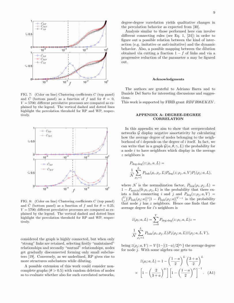
As shown in Fig. 7 (upper panel), when θ = 0, theclustering coefficient relevant to the graph obtained witha random dilution just corresponds, as expected, to thecoefficient pertaining to an analogous ER graph; con-versely, the clustering coefficients for deterministic dilu-tion are larger and display a less trivial profile. In fact,for the RP, starting from small f we first build up a set ofuncorrelated small components having zero or very smallcoefficient, so that their contribution to C is negligible; asignificant and regular increase in C is only set up fromthe percolation threshold (dashed line in the figures).

As for the WP, starting from small f we first connectnodes having strings with large ρ and these form a highlyclustered component which already contributes to C; as fis increased the largest component gradually expands andC consistently grows; when f & fc most nodes are con-nected and new links serve to connect low-degree nodesso that the rate of growth of C is reduced; finally, whenthe network is connected (no isolated nodes) all new linksdetermine an improvement in the clustering so that thereis an acceleration in the growth of C.

Similar arguments apply for the SP percolation: forsmall f only very weak ties are introduced and these,due to the relatively homogeneity of the graph (a = 0),

7

780 880 9800

175

350

s=16954

s=2

ρ

N(ρ

,s)

a)

780 880 9800

90

185

s=2

s=1

s=8812

ρ

N(ρ

,s)

b)

780 880 9800

110

220

s=1

s=3

s=2

ρ

N(ρ

,s)

c)

780 880 9800

175

350

s=17485

ρ

N(ρ

,s)

d)

780 880 9800

175

350

s=14232

s=1

ρ

N(ρ

,s)

e)

780 880 9800

175

350

s=1654

s=1

ρ

N(ρ

,s)

f)

780 880 9800

175

350

s=17472

ρ

N(ρ

,s)

g)

780 880 9800

175

350

s=11938

s=1

ρ

N(ρ

,s)

h)

780 880 9800

175

350

s=1

s=2

ρ

N(ρ

,s)

i)

FIG. 5: (Color on line) Number of nodes N(ρ, s) corresponding to a string with ρ non-null entries and belonging to a clusterof size s, plotted as a function of ρ, while different values of s and shown in different colors. The system considered has sizeV = 17500, θ = 0, α = 0.1 and γ = 1. The nine panels are arranged in such a way that each row represents a different dilutionprocess (from top to bottom: RP, WP, SP), while each column represents a different regime (from left to right: f < fc, f ≈ fc,f > fc).

are sufficient to build up a structures component whichprogressively grows determining a larger and larger C.

In Fig. 8 we show results for the case θ = 0.25; due tothe finite-size effects affecting SP, we just focus on thecases RP and WP. Of course, for the RP no qualitativechanges are evidenced with respect to the case θ = 0,while for the WP, as f is increased, detached small clus-ters are now more likely to occur due to the sparsity ofnon-null entries in strings and this explains the fact thatC is now qualitatively comparable with the ER case.

Another interesting coefficient which we introduce, inorder to monitor the evolving topology as links are re-moved, is a slightly modified version of the clusteringcoefficient, which we denote as C and define as the av-erage of the local dilution Ci, given by the fraction oflinks within the subgraph containing the node i and allits neighbors, that is

C =1

V

V∑i=1

Ci =1

V

V∑i=1

2Eizi(zi + 1)

, (11)

where Ei is the number of links connecting any couple of

nodes belonging to the subgraph, including i itself, andone conventionally sets C = 0 for zi = 0. We remark thatCi differs from Ci by the fact that here we count all linkswithin the neighborhood of i, including those stemmingfrom i, i.e. Ei = Ei+zi, from which Ci = Ci+

∑i 2/(zi+

1). Hence, once f fixed, by comparing C and C, onecan derive information about the arrangement of existinglinks: either highly clusterized, so to form a small-sizedconnected component with nodes having relatively largedegree (comparable C and C) or highly scattered, so toeventually form a large connected component with nodeshaving relatively small degree (large C, small C).

As shown in Fig. 7, again for θ = 0 qualitative differ-ences emerge between deterministic and random dilution.For deterministic percolations C follows a behavior simi-lar to C: this results from the fact that, basically, we haveonly one component which keeps on growing as f is in-creased, the remaining nodes being mainly isolated. Viceversa, for random percolation we can distinguish threedifferent regimes, demarcated by two extremal points: inthe first regime we have the emergence of several smallcomponents (e.g. dimers, trimers), each with small but

8

45 78 1100

425

850

s=1

s=16803

ρ

N(ρ

,s)

a)

45 78 1100

225

450

s=2

s=1

s=9007

ρ

N(ρ

,s)

b)

45 78 1100

275

550

s=1

s=3

s=2

ρ

N(ρ

,s)

c)

45 78 1100

410

820

s=16735

s=1

ρ

N(ρ

,s)

d)

45 78 1100

360

730

s=12724

s=1

s=2

ρ

N(ρ

,s)

e)

45 78 1100

320

630

s=4648

s=1

s=2

ρ

N(ρ

,s)

f)

45 78 1100

445

890

s=17500

ρ

N(ρ

,s)

g)

45 78 1100

445

890

s=17500

ρ

N(ρ

,s)

h)

45 78 1100

445

890

s=1

ρ

N(ρ

,s)

i)

FIG. 6: (Color on line) Number of nodes N(ρ, s) corresponding to a string with ρ non-null entries and belonging to a clusterof size s, plotted as a function of ρ, while different values of s and shown in different colors. The system considered has sizeV = 17500, θ = 0.25, α = 0.1 and γ = 1. The arrangement of panels is the same as in the previous figure.

non-null contributions to C; in the second regime suchsmall components start to merge and this yields a reduc-tion in C; finally, when the graph has reached a connectedstatus, increasing the number of links can just producean increase in C.

For θ = 0.25, also the WP transition display the samemulti-regime behavior, which confirms the picture above.

VII. CONCLUSIONS AND PERSPECTIVES

In this work we analyzed the evolution, under percola-tion process, of a class of weighted graphs G introducedin [12, 13], whose topological properties arise from imita-tive interaction among nodes and can be properly variedby tuning the parameters (α, θ, γ, L). In particular, herewe fixed α = 0.1, γ = 1 and θ = 0 or θ = 0.25, while thesize (V = L/α is the number of nodes) is varied; such asituation corresponds, for large enough volumes, to fully-connected graphs, still retaining a non-trivial distributionPcoupl(J ;α, θ, γ, L) for the coupling strength J associatedto any link. This allows to perform and compare dif-ferent percolation processes: random (RP, where linksare randomly extracted for deletion), deterministic-weak

(WP, where links are deleted starting from the weak-est ones) and deterministic-strong (SP, where links aredeleted starting from the strongest ones).

Our results highlight that weak ties are the most cru-cial in order to ensure the overall connection of the sys-tem, that is, the size of the largest component starts to besmaller than V when only few (weak) links are deleted.When θ approaches value 0.5 from below (and in thepresence of finite-size effects which affect the skewness ofthe coupling distribution) one can see that the spanningtree underlying G is mostly made up of weak links, whilestrong linkes are unlikely and mainly redundant. Hencethe robustness of G sensitively depends on which ties arethe most prone to failure. The fact that weak ties arefundamental to maintain the whole graph connected isconsistent with the so-called theory of weak-ties [28, 29],according to which, in social systems, weak ties work asbridges between different sub-communities.

Moreover, we showed that removing in rank order,from the weakest to the strongest ties, shrinks the net-work, but does not precipitously break it apart, in sucha way that the percolation is rather smooth. A similarphenomenon has been evidenced in the context of so-cial networks where, when all “declared friendships” are

9

10−6 10−4 10−2 1000

0.5

1

f

C

CRPCWPCSP

10−6 10−4 10−2 1000

0.5

1

f

C

CRP

CWP

CSP

FIG. 7: (Color on line) Clustering coefficients C (top panel)

and C (bottom panel) as a function of f and for θ = 0,V = 5700; different percolative processes are compared as ex-plained by the legend. The vertical dashed and dotted lineshighlight the percolation threshold for RP and WP, respec-tively.

10−6 10−4 10−2 1000

0.5

1

f

C

10−6 10−4 10−2 1000

0.5

1

f

C

CRP

CWP

CRP

CWP

FIG. 8: (Color on line) Clustering coefficients C (top panel)

and C (bottom panel) as a function of f and for θ = 0.25,V = 5700; different percolative processes are compared as ex-plained by the legend. The vertical dashed and dotted lineshighlight the percolation threshold for RP and WP, respec-tively.

considered the graph is highly connected, but when only“strong” links are retained, selecting firstly “maintained”relationships and secondly “mutual” relationships, nodesget gradually disconnected forming only small subclus-ters [19]. Conversely, as we underlined, RP gives rise tomore structures subclusters while diluting.

A possible extension of this work could consider non-complete graphs (θ > 0.5) with random deletion of nodesso to evaluate whether also for such correlated networks,

degree-degree correlation yields qualitative changes inthe percolation behavior as expected from [30].

Analysis similar to those performed here can involvedifferent connecting rules (see Eq. 1, [24]) in order tofigure out a possible relation between the kind of inter-action (e.g. imitative or anti-imitative) and the dynamicbehavior. Also, a possible mapping between the dilutionobtained via cutting a fraction 1 − f of links and via aprogressive reduction of the parameter a may be figuredout.

Acknowledgments

The authors are grateful to Adriano Barra and toDaniele Del Sarto for interesting discussions and sugges-tions.This work is supported by FIRB grant RBFR08EKEV .

APPENDIX A: DEGREE-DEGREECORRELATION

In this appendix we aim to show that overpercolatednetworks G display negative assortativity by calculatinghow the average degree of nodes belonging to the neigh-borhood of i depends on the degree of i itself. In fact, wecan write that in a graph G(α, θ, γ, L) the probability fora node i to have neighbors which display in the averagez neighbors is

Pdeg-deg(z; ρi, a, L) =

1

N

L∑ρj=1

Plink(ρi, ρj , L)Pdeg(z; ρj , a, V )P1(ρj ; a, L),

where N is the normalization factor, Plink(ρi, ρj , L) =1 − Pmatch(0; ρi, ρj , L) is the probability that there ex-ists a link connecting i and j and Pdeg(z; ρj , a, V ) =(Vz

)[Plink(ρj ; a)]z[1 − Plink(ρj ; a)]V−z is the probability

that node j has z neighbors. Hence one finds that theaverage degree for i’s neighbors is

z(ρi; a, L) =

V∑z=0

Pdeg-deg(z; ρi, a, L)z =

1

N

L∑ρj=1

Plink(ρi, ρj , L)P1(ρj ; a, L)z(ρj ; a, L, V ),

being z(ρj ; a, V ) = V {1−[(1−a)/2]ρj} the average degreefor node j. With some algebra one gets to

z(ρi; a, L) = 1−(

1− a2

)L(3 + a

2

)L×[1−

(2

3 + a

)ρi] [1−

(1− a

2

)ρi]−1. (A1)

10

Now, noticing that 0 < (1−a)/2 < 2/(3+a) < 1, we candeduce that z(ρi; a, L, V ) is decreasing with ρi, namelywith z(ρi; a, L, V ), so that, as long as the mean-field ap-proach developed here is valid [12, 13], the graph displaysdissortativity.

APPENDIX B: ANALYTICAL RESULTS ON RP

The percolation problem has been studied over differ-ent kinds of structure, both analytically and numerically[31, 32]; in particular, within the so-called configurationmodel approach [33, 34], we can exploit the generatingfunction formalism to get some insights into the problem.First of all, being Pdegree(k) the average degree distribu-tion for the generic graph G (here we drop the dependenceon the parameter set to lighten the notation), we define

G0(x) =

∞∑k=0

Pdegree(k)xk, G1(x) =

∞∑k=0

Q(k)xk, (B1)

where Q(k) = (k + 1)Pdegree(k + 1)/z. Now, as-suming V large and the clustering not significantly,Q(k) is the so-called excess degree [34], represent-ing the degree distribution of the vertex at the endof a randomly chosen edge; notice that G′0(1) = zand G1(x) = G′0(x)/z. Recalling that Pdegree(k) =∑Lρ=0

(Vk

) [1−

(1−a2

)ρ]k ( 1−a2

)ρ(V−k)P1(ρ; a, L), (see

[12, 13]), we can write

G0(x) =

L∑ρ=0

P1(ρ; a, L)

[x+ (1− x)

(1− a

2

)ρ]V.

Moreover, for uniform link deletion probability, the meancluster is [35]

s = 1 + fG′0(1) +f2G′0(1)

1− fG′1(1), (B2)

which diverges when 1 − f G′1(1) = 0; this point marksthe percolation threshold of the system: for f > fc =1/G′1(1) a giant component of connected vertices is es-tablished. Therefore, consistently with the Molloy-Reedcriterion [36], when G′1(1) < 1 the graph consists of manysmall components, while when G′1(1) > 1 a giant compo-nent can emerge. Here we find

G′1(1) =G′′0(1)

z=

z

[1− h(a)]2[1− 2h(a) + g(a)] , (B3)

where h(a) = [(3 − 2a − a2)/4]L = p and g(a) = [(1 −a)(5− a2)/8]L. Assuming a = −1 + γ(α/L)θ and posing

γ = γ(α/L)θ/2, we can write

G′1(1) =z

[1− (1− γ2)L]2

[1− 2(1− γ2)L

+ (1− 2γ2 + γ3)L]→

L→∞z, (B4)

0

0.5

1

01

23

4

2

0

2

4

6

8

10

!"

log(

G! 1(1

))

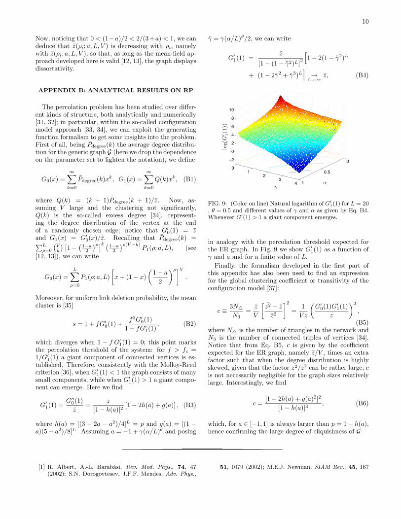
FIG. 9: (Color on line) Natural logarithm of G′1(1) for L = 20

, θ = 0.5 and different values of γ and α as given by Eq. B4.Whenever G′(1) > 1 a giant component emerges.

in analogy with the percolation threshold expected forthe ER graph. In Fig. 9 we show G′1(1) as a function ofγ and a and for a finite value of L.

Finally, the formalism developed in the first part ofthis appendix has also been used to find an expressionfor the global clustering coefficient or transitivity of theconfiguration model [37]:

c ≡ 3N4N3

=z

V

[z2 − zz2

]2=

1

V z

(G′0(1)G′1(1)

z

)2

,

(B5)where N4 is the number of triangles in the network andN3 is the number of connected triples of vertices [34].Notice that from Eq. B5, c is given by the coefficientexpected for the ER graph, namely z/V , times an extrafactor such that when the degree distribution is highlyskewed, given that the factor z2/z2 can be rather large, cis not necessarily negligible for the graph sizes relativelylarge. Interestingly, we find

c =[1− 2h(a) + g(a)2]2

[1− h(a)]3, (B6)

which, for a ∈ [−1, 1] is always larger than p = 1− h(a),hence confirming the large degree of cliquishness of G.

[1] R. Albert, A.-L. Barabasi, Rev. Mod. Phys., 74, 47(2002); S.N. Dorogovtesev, J.F.F. Mendes, Adv. Phys.,

51, 1079 (2002); M.E.J. Newman, SIAM Rev., 45, 167

11

(2003)[2] H.D. Rozenfeld, Structure and Properties of Complex

Networks: Models, Dynamics, Applications (VDM Ver-lag, 2008)

[3] H.J.M. Kiss, A.M. Mihalik, T. Nanasi, B. Ory, Z. Spiro,C. Soti and P. Csermely, BioEssay 31, 651 (2009)

[4] E. Agliari, M. Casartelli and A. Vezzani, J. Stat. Mech.,P10021 (2010).

[5] D. Stauffer and A. Aharony, Introduction to percolationtheory (Taylor & Francis, London 1994)

[6] J.W. Essam, Rep. Prog. Phys. 43, 53 (1980)[7] G. Palla, I. Derenyi, T. Vicsek, Phys. Rev. E 69, 046117

(2004).[8] I. Breskin, J. Soriano, E. Moses, T. Tlusty, Phys. Rev.

Lett. 97, 188102 (2006)[9] L. Huang, Y.-C. Lai, K. Park, J. Zhang, Phys. Rev. E

73, 066131 (2006)[10] Y. Chen, G. Paul, R. Cohen, S. Havlin, S.P. Borgatti, F.

Liljeros, H.E. Stanley, Physica A 378, 11 (2007)[11] M. Brede, U. Behn, Phys. Rev. E 67, 031920 (2003)[12] A. Barra, E. Agliari, Equilibrium statistical mechanics on

correlated random graphs, J. Stat. Mech. P02027 (2011)[13] E. Agliari, A. Barra, A Hebbian approach to complex net-

work generation, Europhys. Lett. 94 10002 (2011)[14] E. Bullmore, O. Sporns, Nature 10, 186 (2009)[15] T. Yamada, P. Bork, Nature 10, 791 (2009)[16] C. Zhao, Intelligent Computing and Information Science

135, 124 (2011)[17] L.M. Sander, C.P. Warren, I.M. Sokolov, Physica A 325,

1 (2003)[18] H.-B. Hu, X.-F. Wang, Europhys. Lett. 86, 18003 (2009)[19] D. Easley, J. Kleinberg, Networks, Crowds, and Markets,

Cambridge University Press (2010)[20] D.J. Amit, Modeling brain functions. The world of at-

tractor neural networks, (Cambridge Press, 1988).[21] R.A. da Costa, S.N. Dorogovstev, A.V. Goltsev, J.F.F.

Mendes, archive:1009.2534.[22] P. Erdos, A. Renyi, Publicationes Mathematicae 6,

290297 (1959).[23] R. Albert, H. Jeong, A.-L. Barabasi, Error and attack

tolerance of complex networks, Nature 79 378 (2000)[24] A. Barra and E. Agliari, Statistical mechanics approach

to autopoietic immune networks, J. Stat. Mech. P07004(2010).

[25] J.-P. Onnela, J. Saramaki, J. Hyvonen, G. Szabo, D.Lazer, K. Kaski, J. Kertesz and A.-L. Barabasi, PNAS104, 7332 (2007)

[26] B. Bollobas, Random graphs, Cambridge UniversityPress, Cambridge (2001)

[27] G. Bianconi, Phys. Rev. E 79, 036114 (2009).[28] M.S. Granovetter, The Strength of Weak Ties, Amer. J.

of Sociology 78, 1360 − 80, (1973).[29] A. Barra, E. Agliari, A statistical mechanics approach to

Granovetter theory, to appear on Physica A.[30] M.E.J. Newman, Assortative Mixing in Networks, Phys.

Rev. Lett., 89, 208701 (2002)[31] G.R. Grimmett, Percolation, Spinger-Verlag, Berlin

1999.[32] B. Bollobas, O. Riordan Percolation, Cambridge Univer-

sity Press, Cambridge 2006.[33] R. Albert and A.-L. Barabasi, Statistical mechanics of

Complex Networks, Rev. Mod. Phys. 74, 47-98 (2002),and references therein

[34] M.E.J. Newman, The structure and function of complexnetworks, SIAM Review, 45, 167-256 (2003), and refer-ences therein

[35] D. Callaway, M.E.J. Newman, S.H. Strogatz, D.J. Watts,Network robustness and fragility: Percolation on randomgraphs, Phys. Rev. Lett. 85, 5468 (2000).

[36] M. Molloy and B. Reed, The size of the giant componentof a random graph with a given degree sequence, Combi-natorics, Probability and Computing 7, 295-305 (1998)

[37] M.E.J. Newman, D.J. Watts, S.H. Strogatz, Proc. Nat.Am. Soc., 99, 2566 (2002)