Percolation, Connectivity, Coverage and Colouring of Random Geometric Graphs

Percolation, connectivity, coverage andcolouring of random geometric graphs

Paul Balister, Bela Bollobas, and Amites Sarkar

Abstract In this review paper, we shall discuss some recent results concern-ing several models of random geometric graphs, including the Gilbert discmodel Gr , the k-nearest neighbour model Gnn

k and the Voronoi model GP .Many of the results concern finite versions of these models. In passing, weshall mention some of the applications to engineering and biology.

1 Introduction

Place a million points uniformly at random in a large square and connect ev-ery point to the six points closest to it. What can we say about the resultinggraph? Is it connected, and, if not, does it contain a connected componentwith at least a hundred thousand vertices? In this paper, we consider suchquestions for some of the most natural models of a random geometric graph,including the one above. From a practical point of view, these graphs are ex-cellent models for ad-hoc wireless networks, in which some radio transceiverslie scattered over a large region, and where each transceiver can only com-municate with a few others nearby. From a more mathematical standpoint,the models act as a bridge between the theory of classical random graphs [16]

Paul BalisterDepartment of Mathematical Sciences, University of Memphis, Memphis, TN 38152, USA.e-mail: [email protected]

Bela BollobasDepartment of Pure Mathematics and Mathematical Statistics, University of Cambridge,Cambridge CB3 0WB, UK, and Department of Mathematical Sciences, University of Mem-phis, Memphis, TN 38152, USA. e-mail: [email protected]

Amites SarkarDepartment of Mathematics, Western Washington University, Bellingham, WA 98225,USA. e-mail: [email protected]

1

2 Paul Balister, Bela Bollobas, and Amites Sarkar

and that of percolation [17], and our study of them will draw inspiration anduse tools from both these more established fields. (It is tempting to write“older” fields, but in fact Gilbert’s pioneering papers [30, 31] appeared onlyshortly after those of Broadbent and Hammersley on percolation, and thoseof Erdos and Renyi on random graphs.)

For all the models, we will take the vertex set to be a unit intensity Poisson

process P in R2, or the restriction of P to a square, so it is convenient to

make some remarks about this at the outset. All our finite results will carryover to the case of uniformly distributed points, but for their proofs, and forthe statements of our infinite results, it is far better to use a Poisson process.

There are several ways of defining such a process, of which the following isperhaps the easiest to describe. First recall that a Poisson random variable

of mean λ is a discrete random variable X for which

P(X = k) = e−λ λk

k!.

As is usual, we will denote this by X ∼ Po(λ). Now tessellate R2 with unit

squares, and consider a family (Xi) of independent random variables, indexedby the squares, where each Xi ∼ Po(1). We place Xi points uniformly atrandom in the square i. The result is a unit intensity Poisson process P .

One of the key features of this model is its independence: the number ofpoints of P in a measurable region A ⊂ R

2 is a Poisson random variable withmean |A| (the Lebesgue measure of A), regardless of what is happening out-side A. Moreover, conditioned on there being k points in A, their distributionis uniform. See [17] for more background.

Throughout the paper, the phrase “with high probability” will mean “withprobability tending to one as n → ∞”. Also, all logarithms in this paper areto the base e.

2 The Gilbert disc model

Our first model was introduced and studied by E.N. Gilbert in 1961 [30], andhas since become known as the disc model or Gilbert model. To define it,fix r > 0, let P be a Poisson process of intensity one in the plane R

2, andconnect two points of P by an edge if the distance between them is less thanr. Denote the resulting infinite graph by Gr.

2.1 Percolation

Although Gilbert’s main focus was the study of communications networks,he noted that Gr could also model the spread of a contagious disease. For the

Percolation, connectivity, coverage and colouring of random geometric graphs 3

second application, and perhaps also for the first, one is primarily interestedin percolation, in the following sense. Let us suppose that, without loss ofgenerality, the origin is one of the points of P . Writing a = πr2, and θ(a) forthe probability that the origin belongs to an infinite connected component ofGr, Gilbert defined the critical area ac as

ac = sup{a : θ(a) = 0}.

In other words, for a > ac, there is a non-zero probability that the diseasespreads, or that communication is possible to some arbitrarily distant nodesof the network. In this case we say that the model percolates. Since θ(a) isclearly monotone, θ(a) = 0 if a < ac. Currently the best known bounds, dueto Hall [35], are

2.184 ≤ ac ≤ 10.588,

although in a recent paper Balister, Bollobas and Walters [12] used 1-independent percolation to show that, with confidence 99.99%,

4.508 ≤ ac ≤ 4.515,

which is consistent with the non-rigorous bounds

4.51218 ≤ ac ≤ 4.51228

obtained by Quintanilla, Torquato and Ziff [49].We can consider the same problem in d dimensions, where we use balls of

volume v rather than discs, and define θd(v) and vdc in the obvious manner.

Penrose [46] proved the following.

Theorem 1.vd

c → 1 as d → ∞.

Most of the volume in a high-dimensional ball is close to the boundary, andhence one might expect that the same conclusion holds for a two-dimensionalannulus where the ratio of the inner and outer radii tends to 1. This is indeedtrue, and was proved independently by Balister, Bollobas and Walters [11]and Franceschetti, Booth, Cook, Meester and Bruck [27]. However, as shownin [11], the corresponding result for square annuli is false. A general conditionunder which the critical area tends to 1 is given in [13].

2.2 Connectivity

Penrose [47, 48] considered the following finite version of Gr. For this, weonly consider points of P lying in a fixed square Sn of area n, again joiningtwo points if the distance between them is less than r. Penrose proved thefollowing result on the connectivity of the resulting model Gr(n).


Theorem 2. If πr2 = log n + α then

P(Gr(n) is connected) → e−e−α

.

In particular, the above probability tends to 1 iff α → ∞.

This result has an exact analogue in the theory of classical randomgraphs [16]. Indeed, in both cases the obstructions to connectivity are iso-lated vertices. In fact, for both models, it is not hard to calculate the expectednumber of isolated vertices, and then to show that their number is has a dis-tribution that is approximately Poisson. The hard part is to show that thereare no other obstructions. For Gr(n), Penrose first shows that the obstruc-tions must be small, that is, of area at most C log n (with our normalization).This he achieves by discretization. Since many of the proofs of the theoremswe will discuss use this technique, we give a brief account of it, for this case.The basic idea is to tessellate our large square with smaller squares of sidelength r/

√5. Any component in Gr(n) must be surrounded by a connected

path consisting of, say, l vacant squares, none of which can contain any pointsof P . Even though the number of such paths of squares is exponential in l, ifthe component is large (so that l ≥ K for some absolute constant K), it is nothard to show that the probability of such a vacant path existing anywherein Sn tends to zero. Thus, with high probability, if Gr(n) is disconnected,it contains a small component. Penrose completes his proof with a delicatelocal argument, showing that, for the relevant range of values of r, this smallcomponent is, with high probability, an isolated vertex.

As shown by Penrose, the story for k-connectivity also mirrors that forclassical random graphs, in that the principal obstructions are vertices ofdegree exactly k. For detailed statements and proofs, the reader is referredto [48].

There are various ways to generalize this model. One, treated thoroughlyin [42], is to choose the disc radii to be independent and identically distributedrandom variables. Another possibility is to keep the radii fixed at r, but varythe intensity of the underlying Poisson process. In one such model, suggestedby Etherington, Hoge and Parkes [23], the intensity ρ(x) of P at distance xfrom the origin is given by a gaussian distribution, so that

ρ(x) = nπ e−x2

.

This model GGaussr (n) was analyzed in detail by Balister, Bollobas, Sarkar

and Walters [7], who determined the threshold for connectivity.

Theorem 3. If

2r√

log n = log log n − 12 log log log n + f(n),

then, with high probability, GGaussr (n) is connected if f(n) → ∞ and discon-

nected if f(n) → −∞.


2.3 Coverage

For most of the remainder of this section, we will imagine that the points ofour Poisson process P are sensors designed to monitor a large square regionSn of area n. Such monitoring is feasible if the sensing discs Dr(p) cover Sn,so that

Sn ⊂⋃

p∈PDr(p).

How large should we make r = r(n) so that this occurs with high probability?Before turning to recent results, we consider the original application of

Moran and Fazekas de St Groth [44]. They considered the problem of coveringthe surface of a sphere with circular caps, and write:

This problem arises in practice in the study of the theory of the manner in which antibodies

prevent virus particles from attacking cells. Thus an influenza virus may be considered to

be a sphere of radius about 40mµ. Antibodies are supposed to be cigar-shaped molecules of

length about 27mµ and of a thickness which will be neglected. The antibodies are assumed

to attach themselves at their ends to the virus particle, standing up rigidly on the surface

and thus shielding a circular area on the virus from possible contact with the surface of a

cell.

Also noteworthy is their simulation method:

...an experiment was carried out using table tennis balls. These had a mean diameter of

37.2mm. with a standard deviation around this mean of 0.02mm. One hundred holes of

diameter 29.9mm. were punched in an aluminium sheet forming one side of a flat box. The

balls were held firmly against the holes by a foam rubber pad, and sprayed with a duco

paint. After drying they were removed and replaced at random by hand. Forty sprayings

were done in each of three sets of 100 balls.

This was also one of the problems considered by Gilbert [31], who per-formed his simulations on an IBM 7094 computer. His paper contains thefollowing critical observation, which we will state in the context of our orig-inal formulation of the problem. For the (open) discs Dr(p) to cover Sn, itis not only necessary but also sufficient that the following three conditionshold:

• Every intersection of 2 disc boundaries inside Sn is covered by a third disc• Every intersection of a disc boundary with ∂Sn is covered by a second disc• There is at least one such intersection (of either type)

Hall [34] used this observation to establish the following criterion.

Theorem 4. If

πr2 = log n + log log n + f(n),


then a necessary and sufficient condition for the discs Dr(p) to cover Sn with

high probability is that f(n) → ∞.

The proof proceeds by showing that if r is as in the statement of Theo-rem 4, then the expected number of uncovered intersections is asymptotically4e−f(n). Thus if f(n) → ∞, by Gilbert’s observation, we obtain coverage withhigh probability. For the other direction, Hall applies the second momentmethod (to the uncovered area).

Slightly later, Janson [37] obtained very general results on the probabilityof coverage. For our case, his result is as follows.

Theorem 5. If

πr2 = log n + log log n + x,

then as n → ∞P(Sn is covered) → e−e−x

.

Recently, a shorter proof of Theorem 5, with bounds on the error term,was obtained by Balister, Bollobas, Sarkar and Walters [10]. The idea is that,while the uncovered intersections occur in groups, these groups consist simplyof the intersections bordering the uncovered regions, which are small (areaC/ logn), and essentially form their own Poisson process of intensity e−f(n).(It is very unlikely that two such uncovered regions are close, because thediscs bordering them are, on their scale, almost half-planes. Moreover, theexpected number of sides of an uncovered region is the same as that of anyother “atomic” region, namely 4. To make these heuristics rigorous, one canuse the Stein-Chen method [2].)

2.4 Colouring

Both Hall [34] and Janson [37] considered not only the case of coverage, butalso that of k-coverage. Our square Sn is said to be k-covered by the discsDr(p) if every point of Sn is contained in at least k discs. This property isuseful for sensor networks, since it allows for the possibility that up to k − 1sensors in a small region might simultaneously fail. Now, in our model, for afixed instance of P , suppose that we increase r until Sn is covered. It turnsout that just a small additional increase in r ensures k-coverage.

Theorem 6 ([10, 37]). For any fixed k ≥ 1, if

πr2 = log n + k log log n + x,

then as n → ∞P(Sn is k-covered) → e−e−x/(k−1)!.


However, suppose we are more optimistic and instead request the following.We would like to devise a rota system so that each sensor can sleep for mostof the time, for example, to extend battery life. A natural way of doing thiswould be to colour the set of sensors with k colours, and arrange that onlythe sensors with colour ℓ are active in the ℓth time slot. After k time slotshave expired, we repeat the process. In order to detect an event occurringanywhere and at any time, it is necessary that the sensors in each colour classthemselves form a single cover of Sn. Thus our question becomes: for fixedk, how large should r be to ensure that the sensors can be partitioned into kgroups, each of which covers the sensing region? We call this the problem ofsentry selection, since each of the groups is a group of sentries keeping watchover the region while the others are sleeping.

It is important to note that a k-cover of an arbitrary set cannot always bepartitioned into k single covers. For instance, let S be the set of all subsetsof A = {1, 2, . . . , n} of size k. The n sets Si = {B ∈ S : i ∈ B}, 1 ≤ i ≤ n,form a k-cover of S which cannot even be partitioned into two single coversif n ≥ 2k− 1. This example shows that a solution to our problem must makesome use of its geometric setting. Also, even restricting ourselves to discsof equal radii, it is possible to construct k-covers of the plane that are not⌈(2k + 2)/3⌉-partitionable. Thus we must also make use of the probabilisticsetting.

Let n, r ∈ R. For k ∈ N, write Ekr for the event that the discs Dr(p) form

a k-cover of Sn, and F kr for the event that they may be partitioned into k

single covers of Sn. Balister, Bollobas, Sarkar and Walters [10] proved thatmost random k-covers are in fact k-partitionable.

Theorem 7. With notation as above,

P(Ekr \ F k

r ) ≤ ck

log n,

for some constant ck.

They also proved that this is sharp, up to a constant. Two hitting timeversions of Theorem 7 are also obtained: if we fix n and slowly increase r, orif we fix r and add points uniformly at random to a given area, then withhigh probability, k-partitionability occurs as soon as we have k-coverage. Inparticular, Theorem 6 holds also for k-partitionability.

Let us suppose that πr2 ≥ log n + (k − 12 ) log log n and attempt to prove

Theorem 7. For this range of values of r, a typical point in Sn is covered atleast log n times. Intuitively, in most of Sn, we can simply colour the discsrandomly, and the probability of failure, that is, of a point x ∈ Sn not beingcovered by discs of every colour, will be negligible. Indeed, if the level ofcoverage is at least 3k log log n everywhere, we can apply the Lovasz locallemma to prove that a suitable colouring exists. However, there will be manyregions in Sn which are covered less than 3k log log n times. Call these thinly

covered regions. It turns out that, with high probability, such regions occur


in small, well-separated clusters. At the scale of the clusters, the curvatureof the discs is negligible, so that they behave like half-planes.

Let us examine one such cluster. We will probably find some very thinly

covered regions, which are covered less than 3k times. These turn out tohave a very useful property (with high probability): some set of k − 1 discsD1, . . . , Dk−1 covers all of them. This facilitates the following simple deter-ministic colouring method. Suppose that all the discs are actually half-planes.Remove the Di, and suppose that we still have a cover of Sn (otherwise, wedid not have a k-cover to begin with). By Helly’s theorem, we can find threeof the half-planes which cover Sn, which we colour with colour k and remove.Now restore Dk−1 and repeat the procedure, colouring three half-planes withcolour k−1 before removing them. Because of the property mentioned above,we can repeat the process k − 2 times, using all the colours, and the levelof coverage in the cluster will never drop to zero until we have finished. Wedo this for every cluster, and, outside the clusters, we complete the colouringusing the Lovasz local lemma, as before.

The actual proofs require somewhat more detailed estimates than theabove sketch suggests. As a by-product, we can identify the principal obstruc-tions to k-partitionability in a k-cover as small non-partitionable k-coveredconfigurations which are covered by k−2 common discs. Since these configu-rations are very small, the curvature of the discs forming them is negligible,so that our obstructions are essentially 2-covers with half-planes which can-not be partitioned into two single covers. It is therefore of interest to classifysuch configurations. Such a classification is presented in [10].

2.5 Thin strips

Suppose that instead of examining points of a Poisson process P inside alarge square, we instead consider the restriction of P to a thin strip T . Asbefore, we will join two points of P at distance less than r. Such a modelwas suggested by the engineering problem of building an electronic “fence”surrounding a large region. The points of P are sensors, and the fence consistsof a thin strip of sensors bordering the region, which has the ability to detectintruders if there is no continuous path crossing it, no point of which lieswithin distance r/2 of any sensor. Note that this is a different condition fromboth connectivity of the underlying graph Gr[T ] of sensors and coverage ofthe sensing regions (of radius r/2). Indeed, if T is a long thin rectangle, ourrequirement is weaker than both connectivity of Gr[T ] and coverage of T by⋃

p∈P∩T Dr/2(p). However, it is not hard to see that the new condition is bothnecessary and sufficient not only for the ability to detect intruders, but alsofor the ability to relay information longitudinally across T , assuming thatthe transmission range of the sensors is r. Informally, if there is a continuous


crossing path γ avoiding all the sensing regions, then the sensors on one sideof γ will be unable to communicate with those on the other side.

To fix ideas, let Th = R × [0, h], and construct the infinite graph Gr[Th].Define a separating path to be a continuous simple path in Th starting atsome point on the line y = h, ending at some point on the line y = 0, andnot passing strictly within distance r/2 of any point of P ∩ Th. This pathwould be a feasible path for an intruder to take in order to avoid detection. Italso identifies a communication breakdown in the information transmissionproblem. We wish to estimate the frequency with which these paths occuralong Th, but some care is needed with the definition of when two such pathsare essentially the same. To this end, we say that a component of Gr[Th] is

good if it contains a vertex strictly within distance√

32 r of the top of Th, and

also a vertex strictly within distance√

32 r of the bottom of Th. The significance

of the factor√

32 is that the good components can be ordered along Th, since

no good component can “jump over” another. Now we may define a break inGr[Th] to be a partition of the good components into two classes: those onthe left of the break and those on the right. It is not hard to see that anyseparating path defines a break, and conversely that, given a break, thereexists a separating path which separates the components on each side of thebreak. However, two separating paths γ1 and γ2 may correspond to the samebreak. The point of this definition is that the breaks count separating pathsthat are essentially different.

s t

a b

Fig. 1 A break between two good components. Figure taken from [3].

Horizontal translation is an ergodic transformation on the probabilityspace of this model, and consequently it is possible to define the intensityIh,r of breaks along Th. (In fact, this can also be seen directly.) Looselyspeaking, a long section of Th of length ℓ will contain approximately ℓIh,r

breaks. Our problems thus reduce to the single problem of estimating Ih,r.This was done by Balister, Bollobas, Kumar and Sarkar [3, 5].

Theorem 8. The intensity of breaks I(h, r) is given by

Ih,r = r1/3ε(hr−1/3) exp(−hr + O(hr−5/3)),


where

log ε(z) = αz + β + oz(1).

Numerical simulations give α ≈ 1.12794 and β ≈ −1.05116. The proof islong and complicated, so we shall content ourselves with a very brief outline.First, a discretization argument shows that, for moderately large values ofr and h, the breaks are typically narrow, that is, they tend to cut straightacross Th and have width Θ(r). Next, a version of Theorem 8 is obtained

for h ≤√

32 r. This involves, among other things, an area-preserving rescaling

of Th near a break, which approximates disc boundaries by parabolas andenables us to replace the two parameters r and h by the single parameterz = hr−1/3. (We also make use of a quantitative version of Perron’s theoremfor eigenvalues of strictly positive matrices.) To extend this to larger valuesof h, we require two additional lemmas. The first is a technical lemma onthe typical shape of a break: loosely speaking we require that most breaksare “rectangular”. The second lemma states that Ih,r is approximately mul-tiplicative, in the sense that if r ≥ 6 and h = h1 + h2 with h1, h2 ≥ r, thenthere is some c > 0 such that

cr−1Ih1,rIh2,r ≤ Ih,r ≤ 50hIh1,rIh2,r.

Naturally, the proof of this begins by splitting the strip Th into two stripsTh1

and Th2, but many difficulties arise at the interface, and we also require

our bound on the expected width of a break established earlier.For many applications, it is useful to know information about the distribu-

tion of the breaks, rather than simply their expected number. It is possible toshow, using the Stein-Chen method [2], that for r ≥ 6 and x > 0, the proba-bility that Gr[Th] restricted to [0, x/Ih,r] contains exactly k breaks tends toe−xxk/k! as h → ∞. For this, we need to know that, for large values of h,the good components are typically wide, and this necessitates a somewhatelaborate discretization argument, owing to complications arising from tilesof our discretization intersecting previously examined regions. For details,see [3].

3 The k-nearest neighbour model

Our second model is very similar to the first. As before, we begin with aPoisson process P of intensity one in the plane R

2. This time, however, wejoin each point p ∈ P to its k nearest neighbours: those points of P which arethe closest, in the usual euclidean norm, to p. (With probability one, there areno ties.) Initially, this creates a directed graph with out-degree k: however, weconvert this into an undirected graph by removing the orientations. Note thatwhile the maximum degree of the resulting graph Gnn

k may be significantlymore than k, the average degree is certainly between k and 2k, and it is not


hard to see (from elementary properties of the Poisson distribution) that, ask → ∞, the average degree is (1 + o(1))k. The maximum degree is at most6k [43].

This is also a very natural model for a transceiver network: one can imag-ine, for instance, that each transceiver can initiate a connection with at mostk others. Indeed, this was the original application, and as such was studiedin a series of papers in the engineering literature (see [61] and the referencestherein).

3.1 Percolation

Percolation in this model is defined as for the Gilbert model, one differencebeing that k is an integer, so that there is some hope of determining thepercolation threshold exactly. To be precise, suppose that the origin is oneof the points of P , write θnn(k) for the probability that the origin belongs toan infinite connected component of Gnn

k , and define kc by the formula

kc = min{k : θ(k) > 0}.

Simulations [6] suggest that θnn(1) = θnn(2) = 0 and that θnn(3) ≈ 0.985, sothat kc = 3, but proving this is another matter. The best published boundsare due to Teng and Yao [52], who show that

2 ≤ kc ≤ 213,

although in a paper to be published, Balister, Bollobas and Walters [14] useda certain oriented 1-independent percolation model to prove that

kc ≤ 11,

and that kc = 3 with confidence 99.99%.As for the Gilbert model, we can consider the same problem in d dimen-

sions. This was done by Haggstrom and Meester [33]. Writing kc(d) for thed-dimensional analogue of kc, they proved that there exists a d0 such that

kc(d) = 2 for all d ≥ d0,

and carried out Monte Carlo simulations which suggest that

kc(d) =

{

3 for d = 2

2 for d ≥ 3.


3.2 Connectivity

Since all transceiver networks are finite, it is natural to consider finite ver-sions of the model Gnn

k . With this in mind, we restrict attention to pointsof P within a fixed square Sn of area n, and ask questions about the graphGn,k formed by joining each point of P within Sn to its k nearest neighbourswithin Sn. Note that this is different from the subgraph of Gnn

k induced by thevertices of P within Sn. One can now ask for an analogue of Penrose’s theo-rem. In other words, how large should we make k = k(n) so as to make Gn,k

connected with high probability? The obstructions to connectivity cannot beisolated vertices, since there are no isolated vertices in our new model: theminimum degree of Gn,k is at least k. On the other hand, it is not hard to seethat, for connectivity, we should look at the range k = Θ(log n). To see this,imagine tessellating the square Sn with small squares Qi of area about log n.Then the probability that a small square contains no points of the process isabout e− log n = n−1, so that, with high probability, every small square con-tains at least one point. A short calculation now shows that, if k ≥ 50 logn,then P(Po(5π log n) > k) = o(n−1), so that, again with high probability, ev-ery point of Gn,k contained in a square Qi is joined to every other point inQi, and also to every point in every adjacent square. This is enough to makeGn,k connected. For a lower bound, imagine a small cluster of k + 1 pointssurrounded by a large annulus containing no points of P . These points willform a component of Gn,k if the thickness of the annulus is greater than the(euclidean) diameter of the cluster it encloses, and if each point outside theannulus has all its k nearest neighbours outside the annulus. It is easy to ex-hibit an example of such a configuration which occurs in a specified locationwith probability e−ck: the constant c depends on the exact specifications ofthe configuration. It is now a simple matter to show that if e−ck ≥ n−c′ forsome c′ < 1 (i.e. if k ≤ c′′ log n for some c′′ < 1/c), such a configuration will,with high probability, occur somewhere in Sn, disconnecting Gn,k.

Define cl and cu by

cl = sup{c : P(Gn,⌊c log n⌋ is connected) → 0},

andcu = inf{c : P(Gn,⌊c log n⌋ is connected) → 1}.

Xue and Kumar [61] were the first to publish bounds on cl and cu: theyobtained cl ≥ 0.074 and cu ≤ 5.1774, although a bound of cu ≤ 3.8597 can beread out of earlier work of Gonzales-Barrios and Quiroz [32]. Subsequently,Wan and Yi [59] showed that cu ≤ e and Xue and Kumar [62] improvedtheir bound to cu ≤ 1/ log 2. The best bounds to date are due to Balister,Bollobas, Sarkar and Walters [6], who proved that cl ≥ 0.3043 and cu ≤1/ log 7 ≈ 0.5139.


In some sense, the lower bound comes from optimizing the shape (andother characteristics) of the cluster of k + 1 points alluded to above. Thedetails are far from straightforward, however, and most of the work consistsof optimizing the region outside the “empty” annulus. For the upper boundin [6], it is important to show first that the obstructions to connectivity aresmall (of area C log n). For this, in turn, one first needs to observe that no twoedges belonging to different components to Gn,k may cross, and indeed that,for k = Θ(log n), any two edges belonging to different components of Gn,k

are, with high probability, separated by a certain minimum distance (whichdepends on k). One can then mimic Penrose’s discretization argument toprohibit the existence of two large components, with high probability. Theremainder of the proof is very different in character and we will not discussit here.

The natural conjecture that cl = cu = c was made in [6] and proved in [9].More precisely, we have the following theorem.

Theorem 9. There exists a constant ccrit such that if c < ccrit and k =⌊c log n⌋ then P(Gn,k is connected) → 0 as n → ∞, and if c > ccrit and

k = ⌊c logn⌋ then P(Gn,k is connected) → 1 as n → ∞.

One of the ideas in the proof of Theorem 9 is that the essentials of a smallcomponent in Gn,k can be captured “up to ε” by a sufficiently fine discretiza-tion (depending on ε but not on k), which can then be scaled for differentvalues of k. The details, however, are complicated. The proof suggests thatc = “0.3043” (where “0.3043” refers to the bound on cl from [6] mentionedabove). To some extent, this is backed up by simulations [6].

From the above results, it follows from the theorems in [8] that also cl =cu = c for the problem of s-connectivity, for any fixed s. For information onthe directed model Dn,k, related coverage problems, and several conjectures,see the papers [6, 8].

3.3 Sharp thresholds

We have seen that, for the Gilbert model, very precise results are knownabout the nature of the transition from non-connectivity to connectivity.For the k-nearest neighbour model, the picture is much less clear, since theobstructions to connectivity are only conjectural. Writing

p(n, k) = P(Gn,k is connected),

let us fix n and focus on the case k ≈ c log n, where c is the critical constantfrom the previous section. We would like to know how quickly p(n, k) changesfrom almost 0 to almost 1 as k increases. Specifically, write

kn(p) = min{ k : p(n, k) ≥ p }.


It seems very likely that, for any 0 < ε < 1, there exists C(ε) such that, forall sufficiently large n,

kn(1 − ε) < C(ε) + kn(ε). (1)

However, this is not known. What is known is that, for fixed k, p(n, k) de-creases sharply from almost 1 to almost 0 as n increases. (One has to increasen by a multiplicative factor to make p(n, k) go from 1 − ε to ε, but that isonly to be expected since k ≈ c log n.) Ignoring problems at the boundary, thebasic idea is that if p(n, k) = 1−ε, say, then we can consider the square SM2n

as the union of M2 copies of Sn, each of which contains a small disconnectingcomponent with probability about ε. Consequently,

p(M2n, k) ≈ (1 − ε)M2

< ε,

for a suitable multiplier M = M(ε). In [8], a weak form of (1) is derived fromthis result via a complicated double-counting argument.

4 Random Tessellations

Random tessellations of R3 were introduced into the study of rock formations

by Delesse [21] 160 years ago, and in recent years they have been used to studya great variety of problems from kinetics to polymers, ecological systemsand DNA replication (see, among others, Evans [24], Fanfoni and Tomellini[25], [26], Ramos, Rikvold and Novotny [50], Tomellini, Fanfoni and Volpe[53], [54], and Pacchiarotti, Fanfoni and Tomellini [45]). In this section weshall concentrate on planar tessellations and give a brief review of the resultsconcerning percolation on the two most frequently studied models, the socalled Voronoi and Johnson–Mehl tessellations.

Strictly speaking, it would suffice to discuss the Johnson–Mehl tessellationsonly, since a Voronoi tessellation is just a special Johnson–Mehl tessellation.Nevertheless, as Voronoi tessellations have been studied for much longer andare much more basic than Johnson–Mehl tessellations, we shall discuss themin a separate subsection.

In fact, first we shall describe a rather general tessellation in Rd, a trivial

extension of the one defined by Johnson and Mehl. Suppose that ‘particles’(also called ‘nucleation centres’) arrive at certain times according to somespatial process, which may be deterministic or random. The moment a par-ticle arrives, it starts to grow a ‘crystal’ at a certain pace, which may beconstant or varying, either deterministically, or in a random way, occupy-ing the ‘unoccupied’ space around it as it grows. Whatever space a particleoccupies belongs to that particle or crystal forever.

In this very general model, the crystal of a ‘fast’ particle may well overtakeand surround the crystal formed by an earlier, but ‘slow’ particle, and the


crystal of a particle may well consist of an infinite number of components.Not surprisingly, such a general model does not seem to be of much use.Needless to say, it is easy to define even more general models of crystals: e.g.,we may use different norms rather than the Euclidean.

In the Johnson–Mehl model, all particles have the same constant speed,so the crystals are simply connected regions and a particle arriving in thecrystal of another particle does not even start to form any crystal of its own,so may be ignored. In a Voronoi tessellation the particles not only have thesame speed, but also arrive at the same time.

4.1 Random Voronoi Percolation

Let us start with a slightly different definition of a Voronoi tessellation. Let Zbe a set of points in R

d. (In our terminology above, Z is the set of ‘particles’ or‘nucleation centres’ that grow into ‘crystals’ or ‘tiles’.) For z ∈ Z, let Vz be theclosed ‘cell’ consisting of those points of R

d that are at most as far from z asfrom any other point of Z. In all cases of interest, Z is taken to be a countableset without accumulation points; also, Z is not too ‘lop-sided’: its convex hullis the entire space R

d. In particular, each cell Vz is the intersection of finitelymany closed half-spaces, so is a convex polyhedron with finitely many faces.Trivially, each Vz is the closure of its interior Uz; also the total boundaryof the cells,

⋃

z 6=z′∈Z Vz ∩ Vz′ , has measure 0. The tessellation or tiling of

Rd into the ‘cells’ or ‘tiles’ Vz is the Voronoi tessellation associated with Z.

As we have already remarked, these tessellations were first introduced byDelesse [21] to study the formation of rocks; their mathematical study wasinitiated only a little later by Dirichlet [22] in connection with quadraticforms, and their detailed study was started by Voronoi [58] about sixty yearslater. Today, in mathematics they tend to be called Voronoi tessellations (ortilings), although occasionally they are named after Dirichlet.

In a random Voronoi tessellation the set Z used to define the Voronoi cellsis taken to be a homogeneous Poisson process P on R

d, of intensity 1, say.The choice of the points z ensures that, with probability 1, the tessellationhas no ‘pathologies’ (in fact, is as ‘regular’ as possible): any two cells Vz, Vz′

are either disjoint or share a full (d−1)-dimensional face, and in every vertexof a cell precisely d + 1 cells meet.

Having defined the cells Vz associated with the points z ∈ P , we definea graph GP with vertex set P by joining two vertices by an edge if theircells share a (d − 1)-dimensional face. Now, a random Voronoi percolation

in Rd is simply a site percolation on GP , where GP itself depends on the

random set P . To spell it out, let 0 < p < 1 be a parameter, and assign oneof two states to each vertex of GP , open or closed, such that, given P , eachvertex is open with probability p, and the state of a vertex is independentfrom the set of states assigned to the other vertices. As always, our system


Fig. 2 Part of a random Voronoi tiling in R2. The dots are the points of a Poisson process.

Figure adapted from [18].

is said to percolate if the graph GP contains an infinite path all of whosevertices are open. Equivalently, we may colour a cell black with probabilityp, independently of the colours of the other cells, and colour a point of R

d

black if it belongs to a black cell: then percolation means that the set of blackpoints has an unbounded component.

There is a more user-friendly way of defining random Voronoi percolation:in this approach we take two independent Poisson processes on R

d, P+ andP−, with intensities p and 1−p, respectively. Then P = P+∪P− is a Poissonprocess of intensity 1, P+ is the set of black (open) points, and P− is the setof white (open) points that are used to define Voronoi cells. Define a graphon P+ by joining two of its points z and z′ if there is a path in R

d fromz to z′ which does not go nearer to another point of P = P+ ∪ P− thanto the nearer of z and z′. We have percolation if this graph has an infinitecomponent.

By making use of Kolmogorov’s 0-1 law one can show that, for each 0 <p < 1, the probability of percolation is either 0 or 1. In the first instance, weare interested in the critical probability pc = pc(d) such that for p < pc theprobability of percolation is 0, and for p > pc it is 1.

Unlike in the case of the classical bond and site percolations on lattices, itis not entirely immediate that this critical probability pc(d) is non-trivial, i.e.,0 < pc(d) < 1. A way of showing this is to use (P+,P−) to define appropriate1-independent percolations on Z

d that imply bounds on pc(d). However, inorder to prove better bounds for pc(d), we have to work rather hard.

For large d, Balister, Bollobas and Quas [4] have proved the followingbounds on pc(d). The proof of the lower bound is fairly easy, but that of theupper bound is more difficult.


Theorem 10. If d is sufficiently large then the critical probability pc(d) for

random Voronoi percolation on Rd satisfies

2−d (9d log d)−1 ≤ pc(d) ≤ C2−d√

d log d,

where C is an absolute constant.

Not surprisingly, most of the interest in random Voronoi percolation cen-tres round percolation in the plane. In fact, in one of the early papers onpercolation, Frisch and Hammersley [29] challenged mathematicians to workon problems of this kind. From the late 1970s, much numerical work wasdone on random Voronoi percolation in the plane (see, e.g., Winterfeld,Scriven and Davis [60], Jerauld, Hatfield, Scriven and Davis [38], and Jer-auld, Scriven and Davis [39]). In particular, Winterfeld, Scriven and Davisestimated that the critical probability for random Voronoi percolation in theplane is 0.500±0.010. In spite of this, it was not even proved that the criticalprobability pc(2) is strictly between 0 and 1.

The 1990s brought about substantial mathematical work on randomVoronoi percolation, notably by Vahidi-Asl and Wierman [55, 56, 57], Zvav-itch [63], Aizenman [1], Benjamini and Schramm [15] and Freedman [28]. Ofthese papers, only [63] is about the critical probability: in this paper Zvavitchproved that pc(2) ≥ 1/2.

Even without computer experiments, it is difficult not to guess that thecritical probability pc(2) is exactly 1/2, but a guess like this is very far froma mathematical proof. Such a proof was given by Bollobas and Riordan [18]in 2006.

Theorem 11. The critical probability for random Voronoi percolation in the

plane is 1/2.

Very crudely, the ‘reason why’ the critical probability is 1/2 is ‘self-duality’.For any rectangle R, either there is a ‘black crossing’ from top to bottomor a ‘white crossing’ from left to right. In particular, if p = 1/2 then theprobability that for a given square S there is a black crossing from top tobottom is precisely 1/2. All this is very well, but there are major difficultiesin piecing together such crossings to form appropriate paths.

In fact, ‘self-duality’ is the reason why the critical probability for bondpercolation in the plane is 1/2, but after Harris’s proof [36] ten years passedbefore Kesten [40] could prove the matching upper bound. By now thereare numerous elegant and simple proofs of this fundamental Harris–Kestentheorem (see Bollobas and Riordan [19, 17]), but it seems that there is noeasy way of adapting any of these proofs to random Voronoi percolation,as the technical problems of overcoming ‘singularities’ are constantly in theway. Indeed, in order to prove Theorem 11, Bollobas and Riordan [18] had tofind a much more involved and delicate argument than those used to tacklepercolation on lattices.


To conclude this subsection, let us mention an important question con-cerning random Voronoi percolation in the plane: is it conformally invariant?(Rather than explaining what this question means, we refer the reader to Ben-jamini and Schramm [15] and to Chapter 8 of Bollobas and Riordan [17].) Letus just add that in 1994 Aizenman, Langlands, Pouliot and Saint-Aubin [41]made the famous conjecture that under rather weak conditions percolation inthe plane is conformally invariant. This has been proved for site percolation inthe triangular lattice by Smirnov [51]. Since random Voronoi percolation hasmuch more built-in symmetry than percolation on lattices, like the triangularlattice, it would not be unreasonable to expect that conformal invariance iseasiest to prove in this case. Unfortunately, so far this expectation has notbeen justified.

4.2 Random Johnson–Mehl Percolation

This time we shall consider only Johnson–Mehl percolation in the plane. Letus recall the definition in the simplest case. ‘Particles’ or ‘nucleation centres’arrive randomly on the plane at random times, according to a homogeneousPoisson process P on R

2 × [0,∞), of intensity 1, say. Thus, if z = (w, t) ∈ Pthen at time t a nucleation centre arrives in the point w ∈ R

2. As soon asthis nucleation centre arrives, it starts to grow at speed 1, say, so that bytime t + u it reaches every point x within distance u of w, and claims it forits crystal, provided it had not been claimed by another nucleation centre. Alittle more formally, if a nucleation centre w ∈ R

2 arrives at time t then itscrystal Vz = V(w,t) consists of all points x such that

d2(x, w) + t ≤ d2(x, w′) + t′

for every point z′ = (w′, t′) ∈ P . (Here d2(x, x′) is the Euclidean distanceof x and x′. In defining a cell, we may safely ignore what happens at theboundary: if a point may be claimed by several particles, we may assign it atrandom to any one of them.)

In yet another description of this random tessellation, we keep the pointsz = (w, t) ∈ P themselves, grow them in the space R

3 (rather than theplane), and then slice this tessellation with the plane R

2 ⊂ R3. To spell this

out, define the Johnson–Mehl norm || · ||JM as the ℓ1-sum of the ℓ2-norms onR

2 and R:

||(x1, x2, t)||JM =√

x21 + x2

2 + |t| = ||(x1, x2)||2 + |t|,

and write d = dJM for the corresponding distance. Then the crystal Vz =V (w, t) of the nucleation centre w that arrived at time t is


Vz ={

x ∈ R2 : d

(

(x, 0), z)

= infz′∈P

d(

(x, 0), z′) }

. (2)

Putting it in this way, we see that Johnson–Mehl tessellations of R2 corre-

spond to two-dimensional slices of Voronoi tessellations of R3 with respect to

the somewhat unusual sum-metric dJM.

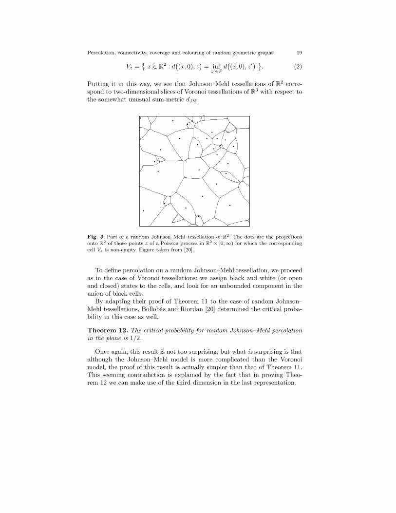
Fig. 3 Part of a random Johnson–Mehl tessellation of R2. The dots are the projections

onto R2 of those points z of a Poisson process in R

2× [0,∞) for which the corresponding

cell Vz is non-empty. Figure taken from [20].

To define percolation on a random Johnson–Mehl tessellation, we proceedas in the case of Voronoi tessellations: we assign black and white (or openand closed) states to the cells, and look for an unbounded component in theunion of black cells.

By adapting their proof of Theorem 11 to the case of random Johnson–Mehl tessellations, Bollobas and Riordan [20] determined the critical proba-bility in this case as well.

Theorem 12. The critical probability for random Johnson–Mehl percolation

in the plane is 1/2.

Once again, this result is not too surprising, but what is surprising is thatalthough the Johnson–Mehl model is more complicated than the Voronoimodel, the proof of this result is actually simpler than that of Theorem 11.This seeming contradiction is explained by the fact that in proving Theo-rem 12 we can make use of the third dimension in the last representation.


5 Outlook

In this brief review we have seen that although in the past fifty years muchwork has been done on properties of random geometric graphs, includingpercolation on them, the subject is still in its infancy. We very much hope thatthe host of beautiful open problems in the area will attract some beautifulsolutions.

References

1. M. Aizenman, Scaling limit for the incipient spanning clusters, in Mathematics ofmultiscale materials (Minneapolis, MN, 1995–1996), IMA Vol. Math. Appl. 99 (1998),1–24.

2. R. Arratia, L. Goldstein and L. Gordon, Two moments suffice for Poisson approxima-tions: The Chen-Stein method, Ann. Probab. 17 (1989), 9–25.

3. P. Balister, B. Bollobas, S. Kumar and A. Sarkar, Reliable density estimates for de-ployment of sensors in thin strips (detailed proofs), Technical Report, University ofMemphis, 2007.Available at http://umdrive.memphis.edu/pbalistr/public/ThinStripComplete.pdf

4. P. Balister, B. Bollobas and A. Quas, Percolation in Voronoi tilings, Random Structuresand Algorithms 26 (2005), 310–318.

5. P. Balister, B. Bollobas, A. Sarkar and S. Kumar, Reliable density estimates for cover-age and connectivity in thin strips of finite length, ACM MobiCom, Montreal, Canada(2007), 75–86.

6. P. Balister, B. Bollobas, A. Sarkar and M. Walters, Connectivity of random k-nearestneighbour graphs, Advances in Applied Probability 37 (2005), 1–24.

7. P. Balister, B. Bollobas, A. Sarkar and M. Walters, Connectivity of a gaussian network,International Journal of Ad-Hoc and Ubiquitous Computing 3 (2008), 204–213.

8. P. Balister, B. Bollobas, A. Sarkar and M. Walters, Highly connected random geometricgraphs, to appear in Discrete Applied Mathematics (2008).

9. P. Balister, B. Bollobas, A. Sarkar and M. Walters, A critical constant for the k-nearestneighbour model, submitted.

10. P. Balister, B. Bollobas, A. Sarkar and M. Walters, Sentry selection in wireless net-works, submitted.

11. P. Balister, B. Bollobas and M. Walters, Continuum percolation with steps in anannulus, Annals of Applied Probability 14 (2004), 1869–1879.

12. P. Balister, B. Bollobas and M. Walters, Continuum percolation with steps in thesquare or the disc, Random Structures and Algorithms 26 (2005), 392–403.

13. P. Balister, B. Bollobas and M. Walters, Random transceiver networks, submitted.14. P. Balister, B. Bollobas and M. Walters, Percolation in the k-nearest neighbour model,

submitted.15. I. Benjamini and O. Schramm, Conformal invariance of Voronoi percolation, Commun.

Math. Phys. 197 (1998), 75–107.16. B. Bollobas, Random Graphs, second edition, Cambridge University Press, 2001.17. B. Bollobas and O.M. Riordan, Percolation, Cambridge University Press, 2006, x +

323pp.18. B. Bollobas and O.M. Riordan, The critical probability for random Voronoi percolation

in the plane is 1/2, Probability Theory and Related Fields 136 (2006), 417–468.


19. B. Bollobas and O.M. Riordan, A short proof of the Harris–Kesten Theorem, Bull.London Math. Soc. 38 (2006), 470–484.

20. B. Bollobas and O.M. Riordan, Percolation on random Johnson–Mehl tessellations andrelated models, Probability Theory and Related Fields 140 (2008), 319–343.

21. A. Delesse, Procede mechanique pour determiner la composition des roches, Ann. desMines (4th Ser.) 13 (1848), 379–388.

22. G.L. Dirichlet, Uber die Reduktion der positiven quadratischen Formen mit dreiunbestimmten ganzen Zahlen, Journal fur die Reine und Angewandte Mathematik40 (1850), 209–227.

23. D.W. Etherington, C.K. Hoge and A.J. Parkes, Global surrogates, manuscript, 2003.24. J.W. Evans, Random and cooperative adsorption, Rev. Mod. Phys. 65 (1993), 1281–

1329.25. M. Fanfoni and M. Tomellini, The Johnson–Mehl–Avrami–Kolmogorov model – a brief

review, Nuovo Cimento della Societa Italiana di Fisica. D, 20 (7-8), 1998, 1171–1182.26. M. Fanfoni and M. Tomellini, Film growth viewed as stochastic dot processes, J. Phys.:

Condens. Matter 17 (2005), R571-R605.27. M. Franceschetti, L. Booth, M. Cook, R. Meester and J. Bruck, Continuum percolation

with unreliable and spread-out connections, Journal of Statistical Physics 118 (2005),721–734.

28. M.H. Freedman, Percolation on the projective plane, Math. Res. Lett. 4 (1997), 889–894.

29. H.L. Frisch and J.M. Hammersley, Percolation processes and related topics, J. Soc.Indust. Appl. Math. 11 (1963), 894–918.

30. E.N. Gilbert, Random plane networks, J. Soc. Indust. Appl. Math. 9 (1961), 533–543.31. E.N. Gilbert, The probability of covering a sphere with N circular caps, Biometrika

56 (1965), 323–330.32. J.M. Gonzales-Barrios and A.J. Quiroz, A clustering procedure based on the compar-

ison between the k nearest neighbors graph and the minimal spanning tree, Statisticsand Probability Letters 62 (2003), 23–34.

33. O. Haggstrom and R. Meester, Nearest neighbor and hard sphere models in continuumpercolation, Random Structures and Algorithms 9 (1996), 295–315.

34. P. Hall, On the coverage of k-dimensional space by k-dimensional spheres, Annals ofProbability 13 (1985), 991–1002.

35. P. Hall, On continuum percolation, Annals of Probability 13 (1985), 1250–1266.36. T.E. Harris, A lower bound for the critical probability in a certain percolation process,

Proc. Cam. Philos. Soc. 56 (1960), 13–20.37. S. Janson, Random coverings in several dimensions, Acta Mathematica 156 (1986),

83–118.38. G.R. Jerauld, J.C. Hatfield, L.E. Scriven and H.T. Davis, Percolation and conduction

on Voronoi and triangular networks: a case study in topological disorder, J. PhysicsC: Solid State Physics 17 (1984), 1519–1529.

39. G.R. Jerauld, L.E. Scriven and H.T. Davis, Percolation and conduction on the 3Dvoronoi and regular networks: a second case study in topological disorder, J. PhysicsC: Solid State Physics 17 (1984), 3429–3439.

40. H. Kesten, The critical probability of bond percolation on the square lattice equals1/2, Comm. Math. Phys. 74 (1980), 41–59.

41. R. Langlands, P. Pouliot and Y. Saint-Aubin, Conformal invariance in two-dimensionalpercolation, Bull. Amer. Math. Soc. 30 (1994), 1–61.

42. R. Meester and R. Roy, Continuum Percolation, Cambridge University Press, 1996.43. G.L. Miller, S.H. Teng and S.A. Vavasis, An unified geometric approach to graph

separators, in IEEE 32nd Annual Symposium on Foundations of Computer Science,1991, 538–547.

44. P.A.P. Moran and S. Fazekas de St Groth, Random circles on a sphere, Biometrika 49

(1962), 389–396.


45. B. Pacchiarotti, M. Fanfoni and M. Tomellini, Roughness in the Kolmogorov–Johnson–Mehl–Avrami framework: extension to (2+1)D of the Trofimov–Park model, PhysicaA 358 (2005), 379–392.

46. M.D. Penrose, Continuum percolation and Euclidean minimal spanning trees in highdimensions, Annals of Applied Probability 6 (1996), 528–544.

47. M.D. Penrose, The longest edge of the random minimal spanning tree, Annals ofApplied Probability 7 (1997), 340–361.

48. M.D. Penrose, Random Geometric Graphs, Oxford University Press, 2003.49. J. Quintanilla, S. Torquato and R.M. Ziff, Efficient measurement of the percolation

threshold for fully penetrable discs, J. Phys. A 33 (42): L399–L407 (2000).50. R.A. Ramos, P.A. Rikvold and M.A. Novotny, Test of the Kolmogorov–Johnson–Mehl–

Avrami picture of metastable decay in a model with microscopic dynamics Phys. Rev.B 59 (1999), 9053–9069.

51. S. Smirnov, Critical percolation in the plane: conformal invariance, Cardy’s formula,scaling limits, Comptes Rendus de l’Academie des Sciences. Serie I. Mathematique,333 (2001), 239–244.

52. S. Teng and F. Yao, k-nearest-neighbor clustering and percolation theory, Algorithmica49 (2007), 192–211.

53. M. Tomellini, M. Fanfoni and M. Volpe, Spatially correlated nuclei: How the Johnson–Mehl–Avrami–Kolmogorov formula is modified in the case of simultaneous nucleation,Phys. Rev. B 62 (2000), 11300–11303.

54. M. Tomellini, M. Fanfoni and M. Volpe, Phase transition kinetics in the case of non-random nucleation, Phys. Rev. B 65 (2002), 140301-1 – 140301-4.

55. M.Q. Vahidi-Asl and J.C. Wierman, First-passage percolation on the Voronoi tes-sellation and Delaunay triangulation, in Random graphs ’87 (Poznan, 1987), Wiley,Chichester (1990), pp 341–359.

56. M.Q. Vahidi-Asl and J.C. Wierman, A shape result for first-passage percolation on theVoronoi tessellation and Delaunay triangulation, in Random graphs, Vol. 2 (Poznan,1989), Wiley-Intersci. Publ., Wiley, New York (1992), pp 247–262.

57. M.Q. Vahidi-Asl and J.C. Wierman, Upper and lower bounds for the route length offirst-passage percolation in Voronoi tessellations, Bull. Iranian Math. Soc. 19 (1993),15–28.

58. G. Voronoi, Nouvelles applications des parametres continus a la theorie des formesquadratiques, Journal fur die Reine und Angewandte Mathematik, 133 (1908), 97–178.

59. P. Wan and C.W. Yi, Asymtotic critical transmission radius and critical neighbor fork-connectivity in wireless ad hoc networks, ACM MobiHoc, Roppongi, Japan (2004).

60. P.H. Winterfeld, L.E. Scriven and H.T. Davis, Percolation and conductivity of randomtw-dimensional composites, J. Physics C 14 (1981), 2361–2376.

61. F. Xue and P.R. Kumar, The number of neighbors needed for connectivity of wirelessnetworks, Wireless Networks 10 (2004), 169–181.

62. F. Xue and P.R. Kumar, On the theta-coverage and connectivity of large randomnetworks, IEEE Transactions on Information Theory 52 (2006), 2289–2399.

63. A. Zvavitch, The critical probability for Voronoi percolation, MSc. thesis, WeizmannInstitute of Science (1996).

Percolation, Connectivity, Coverage and Colouring of Random Geometric Graphs

Documents