Perceptual Audio Coding Sources: Kahrs, Brandenburg, (Editors). (1998). ”Applications of digital signal processing to audio and acoustics”. Kluwer Academic. Bernd Edler. (1997). ”Low bit rate audio tools”. MPEG meeting. Contents: Introduction Requiremens for audio codecs Perceptual coding vs. source coding Measuring audio quality Facts from psychoacoustics Overview of perceptual audio coding Description of coding tools Filterbankds Perceptual models Quantization and coding Stereo coding Real coding systems

Welcome message from author
This document is posted to help you gain knowledge. Please leave a comment to let me know what you think about it! Share it to your friends and learn new things together.
Transcript

Perceptual Audio Coding Sources: Kahrs, Brandenburg, (Editors). (1998). ”Applications of digital
signal processing to audio and acoustics”. Kluwer Academic. Bernd Edler. (1997). ”Low bit rate audio tools”. MPEG meeting.
Contents: q Introduction
q Requiremens for audio codecs
q Perceptual coding vs. source coding
q Measuring audio quality q Facts from psychoacoustics
q Overview of perceptual audio coding
q Description of coding tools q Filterbankds q Perceptual models q Quantization and coding q Stereo coding
q Real coding systems

1 Introduction
n Transmission bandwidth increases continuously, but the demand increases even more à need for compression technology
n Applications of audio coding – audio streaming and transmission over the internet – mobile music players – digital broadcasting – soundtracks of digital video (e.g. digital television and DVD)

Requirements for audio coding systems
n Compression efficiency: sound quality vs. bit-rate n Absolute achievable quality
– often required: given sufficiently high bit-rate, no audible difference compared to CD-quality original audio
n Complexity – computational complexity: main factor for general purpose
computers – storage requirements: main factor for dedicated silicon chips – encoder vs. decoder complexity
• the encoder is usually much more complex than the decoder • encoding can be done off-line in some applications

Requirements (cont.)
n Algorithmic delay – depending on the application, the delay is or is not an important
criterion – very important in two way communication (~ 20 ms OK) – not important in storage applications – somewhat important in digital TV/radio broadcasting (~ 100 ms)
n Editability – a certain point in audio signal can be accessed from the coded
bitstream – requires that the decoding can start at (almost) any point of the
bitstream
n Error resilience – susceptibility to single or burst errors in the transmission channel – usually combined with error correction codes, but that costs bits

Source coding vs. perceptual coding
n Usually signals have to be transmitted with a given fidelity, but not necessarily perfectly identical to the original signal
n Compression can be achieved by removing – redundant information that can be reconstructed at the receiver – irrelevant information that is not important for the listener
n Source coding: emphasis on redundancy removal – speech coding: a model of the vocal tract defines the possible
signals, parameters of the model are transmitted – works poorly in generic audio coding: any kind of signals are
possible, and can even be called music n Perceptual coding: emphasis on the removal of perceptually irrelevant
information – minimize the audibility of distortions

Source coding vs. perceptual coding
n Speech and non-speech audio are quite different – In the coding context, the word ”audio” usually refers to
non-speech audio
n For audio signals (as compared to speech), typically – Sampling rate is higher – Dynamic range is wider – Power spectrum varies more – High quality is more crucial than in the case of speech signals – Stereo and multichannel coding can be considered
n The bitrate required for speech signals is much lower than that required for audio/music

Lossless coding vs. lossy coding
n Lossless or noiseless coding – able to reconstruct perfectly the original samples – compression ratios approximately 2:1 – can only utilize redundancy reduction
n Lossy coding – not able to reconstruct perfectly the original samples – compression ratios around 10:1 or 20:1 for perceptual coding – based on perceptual irrelevancy and statistical redundancy
removal

Measuring audio quality
n Lossy coding of audio causes inevitable distortion to the original signal
n The amount of distortion can be measured using – subjective listening tests, for example using mean opinion score
(MOS): the most reliable way of measuring audio quality – simple objective criteria such as signal-to-noise ratio between the
original and reconstructed signal (quite non-informative from the perceptual quality viewpoint)
– complex criteria such as objective perceptual similarity metrics that take into account the known properties of the auditory system (for example the masking phenomenon)

n MOS – test subjects rate the encoded audio using N-step scale from 1 to 5 – MOS is defined as the average of the subjects’ ratings
n MOS is widely used but has also drawbacks – results vary across time
and test subjects – results vary depending
on the chosen test signals (typical audio material vs. critical test signals)
n Figure: example scale for rating the disturbance of coding artefacts
Measuring audio quality

2 Some facts from psychoacoustics (Recap from Hearing lecture) n Main question in perceptual coding:
– How much noise (distortion, quantization noise) can be introduced into a signal without it being audible?
n The answer can be found in psychoacoustics – Psychoacoustics studies the relationship between acoustic events
and the corresponding auditory sensations
n Most important keyword in audio coding is ”masking” n Masking describes the situation where a weaker but
clearly audible signal (maskee) becomes inaudible in the presence of a louder signal (masker) – masking depends both on the spectral composition of the maskee
and masker, and their variation over time

2.1 Masking in frequency domain
n Model of the frequency analysis in the auditory system – subdivision of the frequency axis into critical bands – frequency components within a same critical band mask each
other easily – Bark scale: frequency scale that is derived by mapping
frequencies to critical band numbers n Narrowband noise masks a tone (sinusoidal) easier than
a tone masks noise n Masked threshold refers to the raised threshold of
audibility caused by the masker – sounds with a level below the masked threshold are inaudible – masked threshold in quiet = threshold of hearing in quiet

Masking in frequency domain
n Figure: masked thresholds [Herre95] – masker: narrowband noise around 250 Hz, 1 kHz, 4 kHz – spreading function: the effect of masking extends to the spectral
vicinity of the masker (spreads more towards high freqencies)
n Additivity of masking: joint masked thresh is approximately (but slightly more than) sum of the components

2.2 Masking in time domain
n Forward masking (=post-masking) – masking effect extends to times after the masker is switched off
n Backwards masking (pre-masking) – masking extends to times before the masker is been switched on
n Figure [Sporer98]: à forward/backward
masking does not extend far in time
à simultaneous masking is more important phenomenon

2.3 Variability between listeners
n An underlying assumption of perceptual audio coding is that there are no great differences in individuals’ hearing
n More or less true – absolute threshold of hearing: varies even for one listener over
time – perceptual coders have to assume very good hearing – masked threshold: variations are quite small – masking in time domain: large variations, a listener can be trained
to hear pre-echos
n Research on hearing is by no means a closed topic – simple models can be built rather easily and can lead to
reasonably good coding results – when desining more advanced coders (perceptual models), the
limits of psychoacoustic knowledge are soon reached
2.4 Conclusion

3 Overview of perceptual audio coding
n Basic idea is to hide quantization noise below the signal-dependent threshold of hearing (masked threshold)
n Modeling the masking effect – most important masking effects are described in the frequency
domain – on the other hand, effects of masking extend only up to about
15ms distance in time (see ”masking in time domain” above)
n Consequence: – perceptual audio coding is best done in time-frequency domain à common basic structure of perceptual coders

3.1 Basic block diagram
n Figure: Block diagram of perceptual audio coding system – upper panel: encoder – lower panel: decoder

Basic block diagram
n Filter bank – used to decompose an input signal into subbands or spectral
components (time-frequency domain) n Perceptual model (aka psychoacoustic model)
– usually analyzes the input signal instead of the filterbank outputs (the preceptual model can be implemented independently of filterbank design)
– computes signal-dependent masked threshold based on psychoacoustics
n Quantization and coding – spectral components are quantized and encoded – goal is to keep quantization noise below the masked threshold
n Frame packing – bitstream formatter assembles the bitstream, which typically
consists of the coded data and some side information

4 Description of coding tools
n In the following, different parts of an audio coder are described in more detail – filter banks used in current systems
à determines the basic structure of a coder – perceptual models
à the algorithmic core of an audio coder – quantization and coding tools
à implements the actual data reduction in an encoder
n Among the additional coding tools, we look briefly at – Stereo/multichannel coding – Spectral band replication

4.1 Filter banks
n Filter bank determines the basic structure of a coder n Example below: block diagram of a static n-channel
analysis/synthesis filterbank [Herre95] – downsampling by factor k at each channel à bandwidths are identical à uniform frequency resolution – critical sampling if k=n

Filter banks: parameters
n Frequency resolution: two main types – low resolution filter banks (e.g. 32 subbands), often called
subband coders: quantization module usually works on blocks in time direction
– high frequency resolution filter banks (e.g. 512 subbands), often called transform coders: quantization module usually works by combining adjacent frequency lines (recent coders)
– Mathematically, all transforms used in audio coding systems can be seen as filter banks (distinction makes no sense theoretically)
n Perfect reconstruction filter banks – enable lossless reconstruction of the input signal in an analysis/
synthesis system, if quantization is not used – simplifies the design of the other parts of a coding system – usually either perfect or near perfect reconstruction filter banks are
used

Filter banks: parameters (cont.)
n Prototype window (windowing of the time frame) – especially at low bit rates, characteristics of the analysis/synthesis
prototype window are a key performance factor
n Uniform or non-uniform frequency resolution – non-uniform frequency resolution is closer to the characteristics of
the human auditory system – in practice, uniform resolution filter banks have been more
successful (simplifies the coder design)
n Static or adaptive filter bank – quantization error spreads in time over the entire synthesis window – pre-echo can be avoided if filter bank is not static but switches
between different time-/frequency resolutions – example: adaptive window switching where the system swithces to
a shorter window in transient-like moments of change

Filter banks in use n Figure: MPEG-1 Audio
prototype LP filter[Sporer98] – polyphase filterbank, 32 bands – window function (top right)
and frequency responses (bottom left and right)
0 0.2 0.4 0.6 0.8 1-120
-100
-80
-60
-40
-20
0
Normalized frequency (Nyquist == 1)
Magnitude Response (dB)
Polyphase Quadrature Mirror Filter Responses

Filter banks in use
n Polyphase filter banks – protype filter design is flexible – computationally quite light – MPEG-1 audio: 511-tap prototype filter, very steep response (see
figure above) – reasonable trade-off between time behaviour and freq resolution
n Transform based filter banks – in practice modified discrete cosine transform (MDCT) nowadays – now commonly used viewpoint: see transform based and
windowed analysis/synthesis system as a polyphase structure where window function takes the role of a prototype filter

Filter banks in use
n Modified discrete cosine transform (MDCT) 1. Window function is constructed in such a way that it satisfies the
perfect reconstruction condition: : h(i)2 + h(i + N/2)2 = 1, i = 0,...,N/2-1, where N is window length
à squared windows sum up to unity if their distance is <win size> / 2 – Why squaring? Because windowing is repeated in synthesis bank.
– sin window and 50% overlap is often used: h(i)=sin[ π(i+0.5)/N ], where i = 0,...,N-1

Filter banks in use
2. Transform kernel is a DCT modified with a time-shift component: where N is freme length, M = N /2 is amount of frequency components, h(n) is window function, xt(n) are samples in the frame t, and Xt(k) are the transform coefficients
– idea of the time-shift component: time-domain aliasing cancellation can be carried out independently for the left and right halves of the window
– compare with normal DCT:
– critical sampling: number of time-frequency components is the same as the original signal samples
– combines critical sampling with good frequency resolution
Xt (k) = h(n)xt (n)cos[π2Nn=0
N−1
∑ (2n+1+M )(2k +1)]
Xt (k) = h(n)xt (n)cosπ2N
⋅2n ⋅2k"
#$%
&'n=0
N−1
∑

Filter banks in use
n Adaptive filter banks – in the basic configuration, time-frequency decomposition is static – adaptive window switching is used e.g. in MPEG-1 Layer 3 (mp3)
n Figure: example sequence – a) long window: normal window type used for stationary signals – b) start window: ensures time domain alias cancellation for the
part which overlaps with the short window – c) short window: same shape as a), but 1/3 of the length à time
resolution is enhanced to 4 ms (192 vs. 592 frequency lines) – d) stop window: same task as that of the start window
n Short windows used around transients for better time reso
a b c d

Pre-echo n In general large number of subbands is beneficial to exploit
masking phenomenon accurately – This results in long analysis windows (dual nature of time/freq.)
n Pre-echo: If coder-generaged artifacts (distortions) are spread in time to precede the signal itself, the resulting audible artifact is called ”pre-echo” – common problem,
since filter banks used in coders cause temporal spreading of
quantization noise within a single frame.
n Figure: Example of pre-echo – lower curve (noise signal)
reveals the shape of the long analysis window

4.2 Perceptual models
n Psychoacoustic model constitutes the algorithmic core of a coding system
n Most coding standards only define the data format – allows changes and improvements to the perceptual model after
the standard is fixed – e.g. ”mp3” format was standardized 1992 but became popular
much later and is still widely used
n Main task of the perceptual model in an encoder is to deliver accurate estimates of the allowed noise
n Additional tasks include 1. control of adaptive window switching (if used) 2. control of bit reservoir (if used) 3. control of joint stereo coding tools

n Strong and prominent components of the signal being encoded hide the noise and distortion resulting from coding.
n Masking thresholds must be inferred from analyzed data. – The masking effect depends on frequency and level
• Generally, masking is asymmetric and spreads more upwards towards higher frequencies. Spread increases with level.
– Tonal masker are different from noise maskers. Noise raises the threshold more than tonal signals with equal power.
– Audio signals contain multiple maskers. n Individual masking curves are combined by summing
masking levels and combined with the threshold of quiet. – Result: Masking threshold curve over the frequency range (for a
single analysis frame).
Perceptual coding

n Given the masked threshold curve, we can maximize quantization noise within each sub-band while keeping noise inaudible (noise shaping)
n Uniform quantization noise within subband decreases 6.02 dB by adding 1 bit. n Figure: the quantization effects the SNR of sub-band. n signal-to-mask ratio SMRN is the band’s capability to mask quantization noise. n Noise is inaudible (perceptual transparency) if SNR > SMR
Perceptual models: bit allocation

Perceptual models: masked threshold n Perceptual models attempt to estimate a time-dependent
signal-to-mask ratio (SMR) for each subband
n Figure: illustration of uniform quantization error in time-domain
– In perceptual audio coding, quantization is performed in time-frequency domain. – transform coefficient scaling to maximum is called ”block companding”, a common scale factor for each subband. – The same quantization step is used for all samples in the same block – Uniform quantization results in noise with flat spectrum
16= 24 levels, 4 bits

Example [Zölzer]: Masking threshold, and signal-to-mask ratio (SMR) at critical bands
Increasing SMR requires more bits Negative SMR requires 0 bits, since signal is masked and does not need to be transmitted

Perceptual models: tonality estimation
n One way to derive a better estimate of the masked threshold is to distinguish between situations where noise masks tone and vice versa
n For complex signals, tonality index v(t,ω) depending on time t and frequency ω leads to best estimate of the masked threshold
n For example, a simple polynomial predictor has been used – two successive instances of magnitude and phase are used to
predict magnitude and phase – distance between the predicted and actual values: the more
predictable, the more tonal

4.3 Quantization and coding n Quantization and coding implement the actual data-
reduction task in an encoder n Remember that quantization is an essential part of
analog-to-digital conversion (along with sampling) – analog sample values (signal levels) are converted to (binary)
numbers
n In coding, digital signal values are further quantized to represent the data more compactly (and more coarsely)
n In perceptual audio coding, quantization is performed in the time-frequency domain (for MDCT coefficient values)
n The quantized values are stored and/or transmitted either directly or as entropy coded words.
n Entropy is a lower bound on the average number of bits needed to represent a set of symbols.

Quantization and coding
n Design options – quantization: uniform or non-uniform quantization (MPEG-1 and
MPEG-2 Audio use non-uniform quantization) – coding: quantized spectral components are transmitted either
directly, or as entropy coded words (e.g. Huffman coding) – quantization and coding control structures (two in wide use): 1. Bit allocation (direct structure): a bit allocation algorithm driven
either by data statistics or by a perceptual model. Bit allocation is done before the quantization.
2. Noise allocation (indirect structure): data is quantized, possibly according to a perceptual model. The number of bits used for each component can be counted only after the process is completed.

Quantization and coding tools
n Noise allocation – no explicit bit allocation – scalefactors of bands are used to colour quantization noise
n Iterative algorithm for noise allocation: 1. quantize data 2. calculate the resulting quantization noise by subtracting
reconstructed signal from the original 3. amplify signal at bands where quantization noise exceeds
masked threshold. This corresponds to a decrease of the quantization step for these bands
4. check for termination (no scaling necessary, or other reason), otherwise repeat from 1

Quantization and coding tools
n Block companding (=”block floating point”) – several values (successive samples or adjacent frequency lines)
are normalized to a maximum absolute value – scalefactor, also called exponent is common to the block – values within the block are quantized with a quant. step selected
according to the number of bits allocated for this block
n Non-uniform scalar quantization – implements ”default” noise shape by adjusting quantization step – larger values quantized less accurately than small ones – for example in MPEG-1 Layer 3 and in MPEG-2 AAC:
where r(i) is original value, rquant(i) is quantized value, quant is quantization step, and round rounds to nearest integer
⎥⎥⎦
⎤
⎢⎢⎣
⎡−⎟
⎠
⎞⎜⎝
⎛= 0946.0
)()(
75.0
quantir
roundirquant
Quantization and coding tools
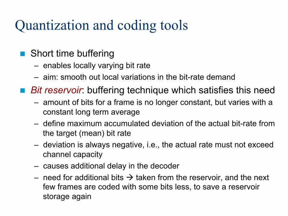
n Short time buffering – enables locally varying bit rate – aim: smooth out local variations in the bit-rate demand
n Bit reservoir: buffering technique which satisfies this need – amount of bits for a frame is no longer constant, but varies with a
constant long term average – define maximum accumulated deviation of the actual bit-rate from
the target (mean) bit rate – deviation is always negative, i.e., the actual rate must not exceed
channel capacity – causes additional delay in the decoder – need for additional bits à taken from the reservoir, and the next
few frames are coded with some bits less, to save a reservoir storage again

Quantization and coding tools
n Figure: example of the bit reservoir technique – note that extra bits are put in earlier frames where some space
has been saved, not to future frames. As a result, the bit rate never exceeds the channel capacity.

4.4 Joint stereo coding n Goal again is to reduce the amount of transmitted
information without introducing audible artifacts n Enabled by exploiting redundancy of stereo signals and
the irrelevancy of certain stereo features – Joint encoding of audio channels should lead to lower bitrate
required to encode the channels separately.
n Redundancy – contrary to intuition, there is usually not much correlation between
the time domain signals of left and right channels – but power spectra of the channels are often highly correlated
n Irrelevancy – human ability to localize sound sources weakens towards high
frequencies – at high frequencies, the spacial perception is mainly based on
intensity differences between channels at each frequency

Joint stereo coding: pitfalls n In some cases, the required bit-rate for stereo coding
exceeds that needed for coding two mono channels – certain coding artifacts which are masked in a single channel
become audible when two coded mono channels are presented à binaural masking level difference (esp. at low frequencies)
n Precedence effect – sound sources are localized according to the first wavefront à coding techniques may result in a distorted stereo image by
introducing timing changes into the first wavefront arrival times.
n Stereo unmasking effect – Certain coding artifacts which are masked in single channel
coding can become audible when presented as a stereo signal coded by a dual mono coding system.
– Maximum masking occurs when the direction of the virtual quantization noise source coincides with the direction of the main signal source.

Mid/Side (M/S) stereo coding n Normalized sum and difference signals are transmitted
instead of left and right channels n Emphasis on redundancy removal n Perfect reconstruction
– altering between L+R ßà M+S does not lose information
n Heavily signal dependent bit-rate gain – varies from 50 % (identical left/righ channel signals) to 0 %
n Preserves spatial information (can be applied to all freqs.) n Figure: block diagram of M/S stereo coding [Herre95]

Intensity stereo coding n For each subband, only one intensity spectrum is retained
– directional information is transmitted by encoding independent scalefactor values for left and right channels
n Rather successful at high frequencies – main spatial cues are transmitted, some details may be missing – less annoying than other coding errors
n Emphasis on irrelevancy removal – 50 % data reduction at high frequencies, approx 20 % for the
entire signal
n Figure: basic principle of intensity stereo coding [Herre95]

n Parametric Stereo (PS) – Extends the concept of intensity stereo coding, operates fullband – Channel data is transmitted as mono downmix with parametric
side-information: Inter-channel level differences (ICLD), inter-channel phase difference (ICPD), and inter-channel coherence ICC* (similarity in time-frequency).
– ICC information enables creation of a wide stereo image
n MPEG Surround and MPEG spatial audio object coding (SAOC) are similar techniques for multi-channel audio
n MPEG Surround can transmit 5.1 surround audio content in stereo or mono downmix channels with spatial metadata.
n MPEG SAOC provides multiple audio objects in the downmix channels with side-information to enable spatial adjustment of audio objects.
Parametric stereo and surround sound
*) ICC= | E[X1X2*] | / (E[ |X1|2 ] × E[ |X1|2 ] ), E[�] is expected value, X1 is 1st channel time-frequency point.

n SBR exploits common large dependencies between the lower and higher frequency parts of an audio signal.
n The high frequency part of a signal is predicted from the transmitted low frequency part and control data (envelope adjustment, additional high-freq. components)
n SBR does not deliver the desired results if there is little relationship between the low and high frequency part.
n The lower part can be transmitted with higher sampling rate. n Figure: from [Dietz02]
4.5 Spectral Band Replication
Masked threshold
transmitted reconstructed
Signal energy

4.6 Huffman coding
n Lossless compression applied to quantised coefficients to remove further redundancy
n Pre-computed tables kept for various codecs n Not used in MPEG-1 layers 1 or 2 n Used in MPEG-1 layer 3 (.mp3) and AAC

5 Real coding systems n MPEG (Moving Pictures Experts Group) standardizes compression
techniques for video and audio n Three low bit-rate audio coding standards have been completed
– MPEG-1 Audio (layers 1, 2, and 3 (”mp3”)) – MPEG-2 Backwards Compatible coding (multichannel, more rates) – MPEG-2 Advanced Audio Coding (AAC)
n MPEG-4 – Consists of a family of coding algorithms targeted for speech,
audio, text-to-speech interfaces, lossless coding. n Codecs outside MPEG
– Ogg Vorbis, Windows Media Audio – Generally similar to the MPEG coders

MPEG-1 Layer 3 (.mp3)
n Figure: block diagram of an MPEG-1 Layer 3 encoder
Related Documents