ALMA MATER STUDIORUM – UNIVERSITÀ DI BOLOGNA SEDE DI CESENA SECONDA FACOLTÀ DI INGEGNERIA CON SEDE A CESENA CORSO DI LAUREA MAGISTRALE IN INGEGNERIA BIOMEDICA “TACTILE PERCEPTION – PERCEPTION OF TACTILE DISTANCE CHANGES WITH BODY SITE: A NEURAL NETWORK MODELLING STUDY.” Tesi in Sistemi Neurali LM Relatore Presentata da Prof.ssa Elisa Magosso Enrico Altini Correlatore Dr. Matthew Longo III SESSIONE ANNO ACCADEMICO 2010/2011

Welcome message from author
This document is posted to help you gain knowledge. Please leave a comment to let me know what you think about it! Share it to your friends and learn new things together.
Transcript
ALMA MATER STUDIORUM – UNIVERSITÀ DI BOLOGNA SEDE DI CESENA
SECONDA FACOLTÀ DI INGEGNERIA CON SEDE A CESENA CORSO DI LAUREA MAGISTRALE IN INGEGNERIA BIOMEDICA
“TACTILE PERCEPTION – PERCEPTION OF TACTILE DISTANCE CHANGES WITH BODY SITE:
A NEURAL NETWORK MODELLING STUDY.”
Tesi in
Sistemi Neurali LM
Relatore Presentata da Prof.ssa Elisa Magosso Enrico Altini Correlatore Dr. Matthew Longo
III SESSIONE
ANNO ACCADEMICO 2010/2011

To my family: Mum, Dad, Erika, Massimo, and my sweet Gaia….
KEY WORDS FOR THIS THESIS:
Ø Computational Model
Ø Synaptic Connections
Ø Tactile Perception
Ø Weber’s Illusion
Index
Introduction
Chapter 1
Tactile Information Processing and Tactile Distance Perception Introduction…………………………………………………………………......5
1.1 Touch…………………………………..……………………………………6
1.2 Mechanoreceptors and Receptive Fields…………………………………...8
1.3 Somatic Sensory Cortex…………………………………………………...11
1.4 Cortical Neuron RF…………………………………………………..........13
1.5 Tactile Illusion: Weber’s Illusion………………………………..………...15
1.5.1 Homunculus………………………………………………………....17
1.5.2 Magnification Concept…………….….…………………….……....19
1.5.3 Green Experiment…………….….…………………….……............23
1.6 The Neural Network and the simplifying assumptions………...….……....19
Chapter 2
Mathematical Model
2.1 Qualitative description of the model……...……………………………….28
2.1.1 The two main layers..………………………………………………..28
2.1.2 Application of 2 punctual stimuli: effects within the First Layer…...31
2.1.3 Application of 2 punctual stimuli: effects within the Second Layer...31
2.2 Mathematical description of the network………………………………….35
2.2.1 First Layer of neurons (Area 1)..…………………………………….36
2.2.2 Second Layer of neurons (Area 2)…..……………………………….40
2.3 Parameters and their values………………………………………………..42
2.4 Activation of neurons step by step……………...…………………………43
2.5 Periodic Domain……………...……………………………………………57
INDEX
II
Chapter 3
Simulations and results Introduction…………………………………………….……………………….62
The noise……………………………………………….……………………….63
Threshold of activation……………………………….…………………………65
3.1 First Experiment…………………………………………………………...66
3.1.1 Tactile Size Perception on the Hand vs Arm …………………..........66
3.1.2 PSE and IQR of the First Experiment………………………….…….71
3.1.3 Activation of neurons in the Hand and in the Arm ………………….75
3.2 Second Experiment………………………………………………...............76
3.2.1 Student t-Test………………………………...………………………76
3.3 Third Experiment………………………………………………..................82
3.3.1 Two Point Discrimination Threshold ………..……………………...82
3.3.2 Comparison with Green’s results……………………………….……92
3.3.3 Rescaling Process results.…………………………………………....93
3.4 Fourth Experiment………………………………………………………....97
3.4.1 Dependency on the stimuli dimension ………..……………………..97
3.4.2 Analysing of Area1’s output…………………………………......…105
3.4.3 Analysing of Area2’s output…………………………………......…105
3.4.4 Validation with t-Test…………………………………......………..106
3.4.4.1 First Layer: mean 3 vs Mean 4…………………………….110
3.4.4.2 Second Layer: mean 3 vs Mean 4………………………….111
Chapter 4
Parameter Sensitivity Analysis 4.1 Parameter Sensitivity Analysis and Reference Results ……………….....113
4.2 The changed Parameters………………………………………………….116
4.2.1 Parameters Alteration……………………………………………...118
4.3 Alteration of the Parameters and Neural Network Behaviour …………...119
4.4 Average Difference between the two activation balls ………...………....139
4.5 Conclusion about the Sensitivity Analysis…………………………….....141
4.6 Sensitivity Analysis about the Activation Threshold………….…………142
4.7 Increment of the Inhibitory Component ………….…………………...…151

INDEX
III
Conclusions…………………………………………………………………………...155
Bibliography ………………………………………………………………………....159
1
INTRODUCTION
Distortions in the perception of the distance between two punctual stimuli
applied on the skin surface of different body regions are called Weber’s
Illusion. This illusion was confirmed by many experiments, in which subjects
were asked to judge the distance between two stimuli applied on the skin surface
of different body regions. Results have shown that the same distance between
the stimuli was judged different for different body regions.
The concept that the distance on the skin is frequently misperceived is largely
supported, but the neural mechanisms underlying this illusion are still far to be
well understood. In particular, it is still unclear how the distance between two
simultaneous tactile stimuli is codified at a neural level, and which brain areas
are involved in this computation.
Weber’s Illusion may be partly explained considering the differences in
receptors density of various body regions, and the distorted image about the
body that our brain has inside the Primary Somatic Sensory Cortex
(homunculus). However, these mechanisms seem not to be sufficient to explain
the observed phenomenon: indeed, according to 100 years-experimental results,
the biases in distance judgement are much smaller than imbalances that primary
representation would suggest. In other words, the observed illusion is much
smaller compared to the effect that the differences in receptor density, or cortical
extent would produce. This has lead to the hypothesis that judging tactile
distance may require the recruitment of additional brain areas, and mechanisms
that operate to rescale – at least partially – information from primary
representation, in order to preserve tactile size constancy throughout the body
surface
That is, it has been proposed the occurrence of sort of “Rescaling Process” that
operates to reduce this illusion toward a more verisimilar perception.
INTRODUCTION
2
The occurrence of this rescaling process is supported by many neuroscience
researchers; in particular, Dr. Matthew Longo from the Department of
Psychological Sciences, Birkbeck University of London is conducting research
on tactile distance perception and body representation, and its research supports
this hypothesis. However, the neural mechanisms and circuits at the basis of this
potential rescaling process are still largely unknown.
The aim of this thesis was to clarify the possible network organization, and
neural mechanisms explaining the Weber’s Illusion and the rescaling process, by
using a neural network model. Much of the work was conducted at the
Department of Psychological Sciences, Birkbeck University of London, under
the supervision of Dr. Matthew Longo.
In order to replicate Weber’s Illusion and rescaling process, the neural network
has been organized in two main layers of neurons that may correspond to two
functionally different cortical areas:
• First Layer of neurons (that performs the first processing of the external
stimuli): this layer might mimic the Primary Somatic Sensory Cortex
affected by cortical magnification.
• Second Layer of neurons (that further elaborates information from the
previous layer): this layer may represent a Higher Cortical Areas (e.g. in
temporo-parietal region) involved in the implementation of the Rescaling
Process.
Neural networks have been constructed including synapses connection within
each neuron layers (lateral synapses), and between the two neural layers (feed-
forward synapses), and assuming that the activity of each neurons depends on its
input via a static sigmoidal relationship, and a first order dynamics. In particular,
by using the previous structure, I have implemented two different neural
networks, for two different body regions (for example, the Hand and the Arm),
characterized by different tactile resolution and cortical magnification to
replicate the Weber’s Illusion and the Rescaling Process.
These models may help to understand the mechanism of the Weber’s Illusion,
and to give a possible explanation of the Rescaling Process. Moreover, the
INTRODUCTION
3
neural networks may help to understand how the brain can interpret the distance
on the skin surface, and these models could be used to make new predictions to
be verified later, in vivo, by tactile experiments on real subjects. It is important
to underline that the developed models are mainly functional models and they
are not intended replicate physiologic and anatomic details.
The main results achieved via the models are the reproduction of the Weber’s
Illusion for the two different considered body regions (Hand and Arm), as
reported in many articles about the tactile illusions. Weber’s Illusion was
recorded from the output of the neural networks, and represented by graphics,
trying to explain the reasons of these results.
The main part of this thesis was developed in the Department of Psychological
Sciences, at Birkbeck, University of London under the supervision of Dr.
Matthew Longo, for a period of 5 months. The contribute of Dr. Longo was very
useful due to his great experience about experiments involved in the tactical
perceptions. His help was directed especially toward the interpretation of the
model outputs, giving suggestions about processing of network results, in order
to obtain clearer information. Moreover, Dr. Longo has provided help in
validation results, performing statistical test. Besides the benefit of interacting
directly with an expert person as Dr. Longo, another benefit of may visit at the
Birkbeck University was the improvement of my English, and the contact with a
different university reality, as well as the experience of working in a team of
researchers.
The present thesis is organized in four chapters.
The first chapter explains the theoretical aspects of the Weber’s Illusion, and the
tactile processing information that starts from the skin surface of a body region,
and continues through different layers in the cortex.
The second chapter is entitled “Mathematical Model”; it explains the network
structure, provides a quantitative description of the model containing all
mathematical formulas, explanation of each parameter, and provides example of
neural activation within the two network layers.
INTRODUCTION
4
Chapter 3 shows the results of the simulations: this chapter provide deep
analyses of the output of the neural network in response to the application of an
input (two punctual stimuli).
Finally Chapter 4 concerns the “Parameters Sensitivity Analysis”: in that
Chapter, simulation results have been analysed after changing the value of one
parameter at a time, in order to assess which parameters mainly affect network
behaviour.
Chapter 1
TACTILE INFORMATION PROCESSING AND TACTILE DISTANCE
PERCEPTION
Introduction
The perception of distance for dual tactile pressures changes for different body
regions. Over a century ago, Weber reported the concept that the distance on the
skin is frequently misperceived. In the Weber’s illusion, the perception of
distance between two tactile punctual stimuli is different in different parts of the
body, increasing as the spatial acuity of the stimulated area increases.
Probably, the main reasons of this Illusion, are relative to the different size of the
Receptive Field (RF) on the skin surface bonded to each cortical neuron, and the
fact that the Primary Somatic Sensory Cortex reserves different amounts of area
for representation of different body regions: for example, the Area involved in
the perception of the hand, is much bigger than the Area about the back or the
arm (homunculus).
Different extensions of cortical surface implicate different resolutions on
different body regions: there are much more neurons in the brain involved to the
hand, than the arm. Thus, the area inside the cortex reserved to the hand is
bigger compare with the arm’s area. This means that the hand has a higher
resolution in the comparison with the arm.
My thesis intends to implement a model able to simulate how the brain can
interpret tactile stimuli on the skin surface in two different body regions. From
the Weber’s experiment the application of two simultaneous stimuli (on the skin
surface with a constant distance, on two different regions (like the hand and the
arm) produce two different perceptions of distance.
TACTILE INFORMATION PROCESSING AND TACTILE DISTANCE PERCEPTION
6
As I stated above, the classical explanation of the Weber’s Illusion is the
difference in the density of tactile receptors and cortical magnification across
body parts. However, this explanation is unsatisfactory, because the illusion is
much smaller than the differences in receptor density or cortical extent.
Therefore, there must be present a sort of rescaling process along the pathways
of tactile information processing in the brain that might decrease this huge
difference (relative to the homunculus dimension) and brings it to an acceptable
proportion. It is clear that we feel a sort of distortion in the perceived distance,
but basically it is kept down.
The neural mechanisms underlying this rescaling process are still largely
unknown. Aim of this thesis is to contribute to clarify the neural mechanisms
that may implement this rescaling, via a neural network modelling study. Of
course, the model includes several simplifications and it doesn’t aspire to
reproduce exactly the reality, also because the number of variables that should
be considered is massive. This is mainly a conceptual model that, with the help
of some hypotheses, tries to reproduce and interpret some experimental
evidences (Weber’s illusion, distortions in perceive distance).
Before starting to explain my model, in this introduction I’m going to introduce
few important concepts about the Receptive Field, the Primary Somatosensory
Cortex, and the Homunculus.
1.1 Touch
Touch is mediated by mechanoreceptors in the skin and the tactile sensitivity is
greatest on the hairless skin (glabrous), on the fingers, palm, sole of the foot and
lips. When an object presses against the hand, the skin conforms to its contours.
All mechanoreceptors sense these changes in skin contour, and they answer with
a particular physiological function that will reach the Somatic Sensory Cortex
inside the Central Nervous System.
TACTILE INFORMATION PROCESSING AND TACTILE DISTANCE PERCEPTION
7
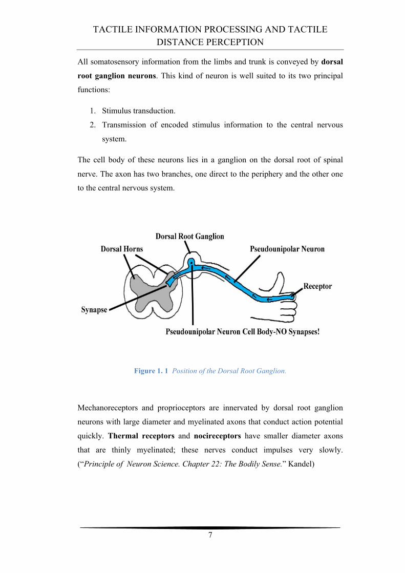
All somatosensory information from the limbs and trunk is conveyed by dorsal
root ganglion neurons. This kind of neuron is well suited to its two principal
functions:
1. Stimulus transduction.
2. Transmission of encoded stimulus information to the central nervous
system.
The cell body of these neurons lies in a ganglion on the dorsal root of spinal
nerve. The axon has two branches, one direct to the periphery and the other one
to the central nervous system.
Figure 1. 1 Position of the Dorsal Root Ganglion.
Mechanoreceptors and proprioceptors are innervated by dorsal root ganglion
neurons with large diameter and myelinated axons that conduct action potential
quickly. Thermal receptors and nocireceptors have smaller diameter axons
that are thinly myelinated; these nerves conduct impulses very slowly.
(“Principle of Neuron Science. Chapter 22: The Bodily Sense.” Kandel)
TACTILE INFORMATION PROCESSING AND TACTILE DISTANCE PERCEPTION
8
Neurologists distinguish between two classes of somatic sensation: epicritic and
protopathic. Epicritic sensations involve aspects of touch and are mediated by
encapsulated receptor. Instead, Protopathic sensation involves pain and
temperature senses, and are mediated by receptors with bare nerve endings.
In this thesis we will concentrate on Epicritic Sensations.
Information transmitted to the brain from mechanoreceptors in the hand, enabled
us to feel the shape and texture of objects, type on computer keyboards, play
musical instruments, etc. The ability to recognize objects placed in the hand on
the basis of touch alone, is one of the most important and complex function of
the somatosensory system. Tactile information about an object is fragmented by
peripheral sensors, and must be integrated by the brain. In fact, an object
stimulates a large number of receptors and sensory nerve fibres, each of which
scans a little part of the object. Spatial properties are processed by populations of
receptors that form many parallel pathways to the brain. It is the job of the
central nervous system to reconstruct the correct shape of the object from the
received fragmented information.
1.2 Mechanoreceptors and Receptive Fields
Mechanoreceptors differ in morphology and skin location. Histological and
physiological studies have identified four major types of mechanoreceptors on
the glabrous skin. Two of these are located in the superficial layers of the skin
(Meissner’s corpuscle and Merkel disk receptor), and the other two in the
subcutaneous tissue (Pacinian corpuscle and Ruffini ending). The small
superficial receptors sense deformation of the papillary ridges in which they
reside. The larger subcutaneous receptors sense deformation of a wider area of
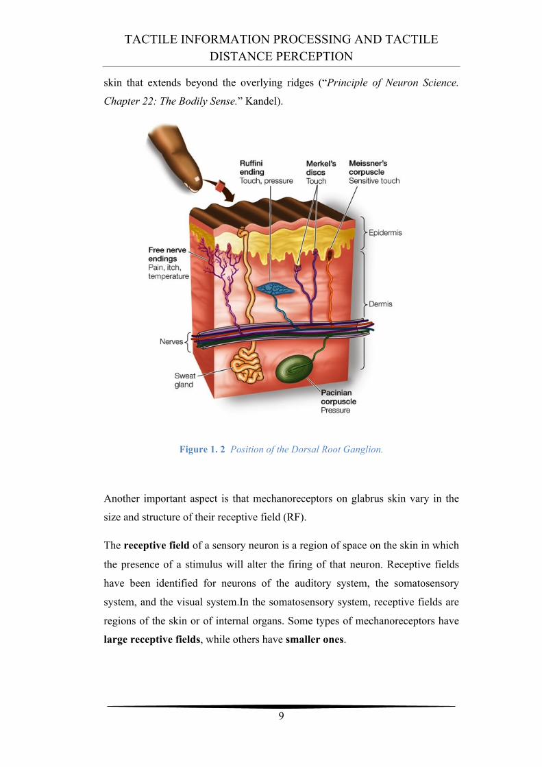
TACTILE INFORMATION PROCESSING AND TACTILE DISTANCE PERCEPTION
9
skin that extends beyond the overlying ridges (“Principle of Neuron Science.
Chapter 22: The Bodily Sense.” Kandel).
Figure 1. 2 Position of the Dorsal Root Ganglion.
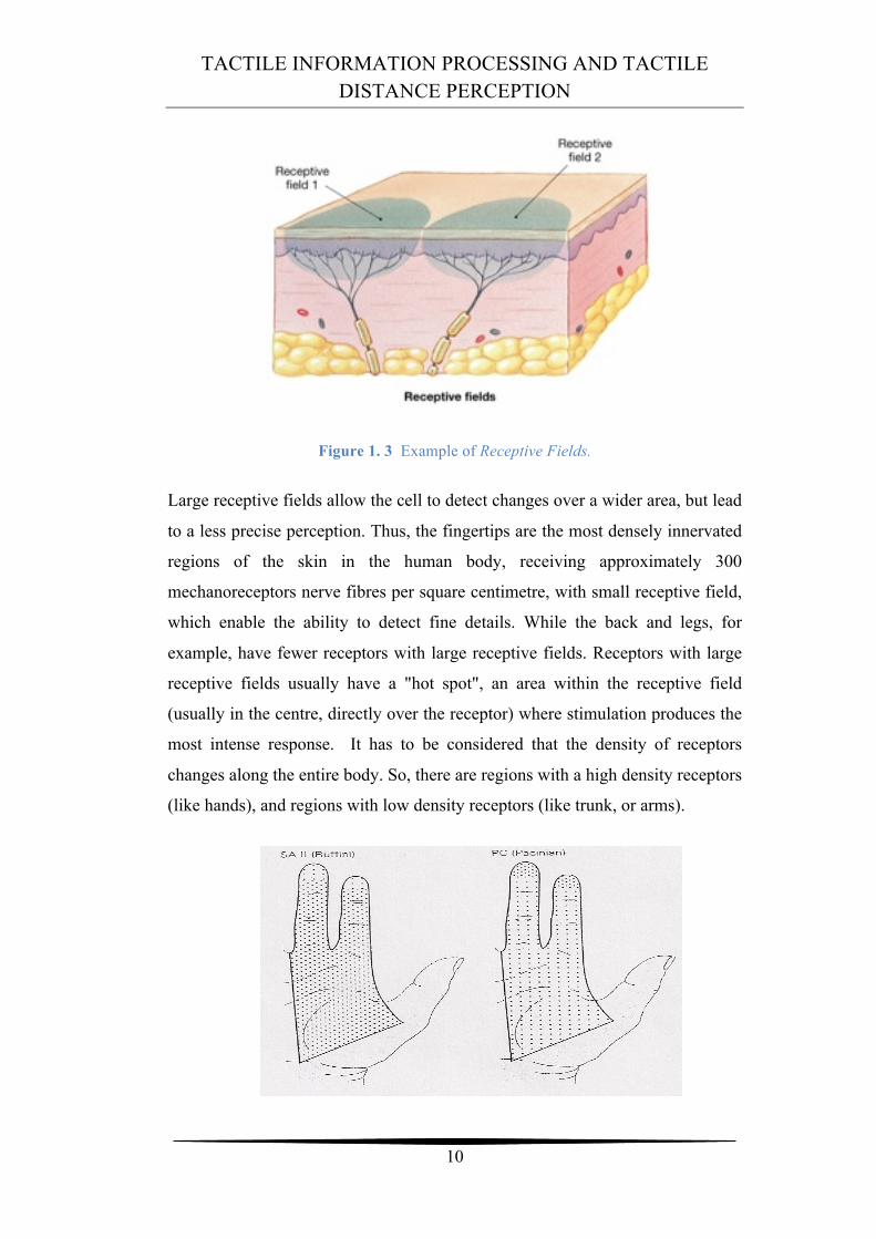
Another important aspect is that mechanoreceptors on glabrus skin vary in the
size and structure of their receptive field (RF).
The receptive field of a sensory neuron is a region of space on the skin in which
the presence of a stimulus will alter the firing of that neuron. Receptive fields
have been identified for neurons of the auditory system, the somatosensory
system, and the visual system.In the somatosensory system, receptive fields are
regions of the skin or of internal organs. Some types of mechanoreceptors have
large receptive fields, while others have smaller ones.
TACTILE INFORMATION PROCESSING AND TACTILE DISTANCE PERCEPTION
10
Figure 1. 3 Example of Receptive Fields.
Large receptive fields allow the cell to detect changes over a wider area, but lead
to a less precise perception. Thus, the fingertips are the most densely innervated
regions of the skin in the human body, receiving approximately 300
mechanoreceptors nerve fibres per square centimetre, with small receptive field,
which enable the ability to detect fine details. While the back and legs, for
example, have fewer receptors with large receptive fields. Receptors with large
receptive fields usually have a "hot spot", an area within the receptive field
(usually in the centre, directly over the receptor) where stimulation produces the
most intense response. It has to be considered that the density of receptors
changes along the entire body. So, there are regions with a high density receptors
(like hands), and regions with low density receptors (like trunk, or arms).
TACTILE INFORMATION PROCESSING AND TACTILE DISTANCE PERCEPTION
11
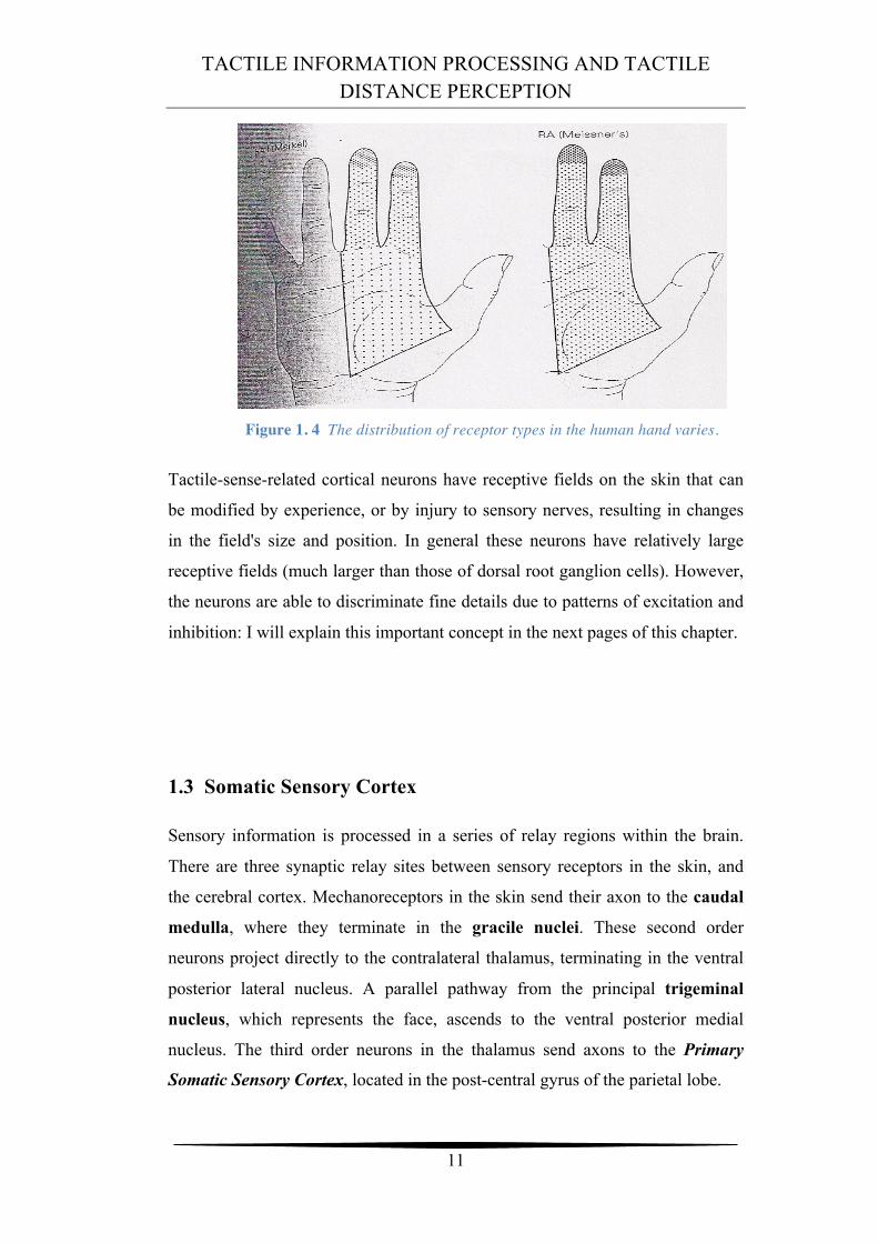
Figure 1. 4 The distribution of receptor types in the human hand varies.
Tactile-sense-related cortical neurons have receptive fields on the skin that can
be modified by experience, or by injury to sensory nerves, resulting in changes
in the field's size and position. In general these neurons have relatively large
receptive fields (much larger than those of dorsal root ganglion cells). However,
the neurons are able to discriminate fine details due to patterns of excitation and
inhibition: I will explain this important concept in the next pages of this chapter.
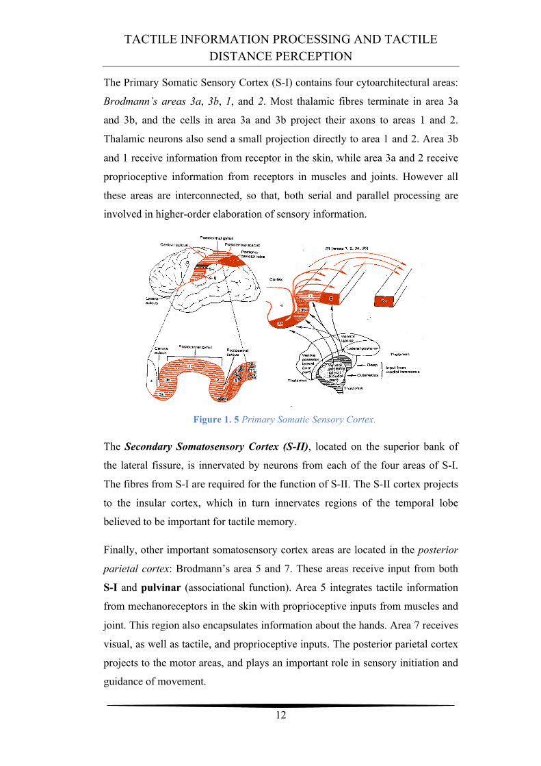
1.3 Somatic Sensory Cortex
Sensory information is processed in a series of relay regions within the brain.
There are three synaptic relay sites between sensory receptors in the skin, and
the cerebral cortex. Mechanoreceptors in the skin send their axon to the caudal
medulla, where they terminate in the gracile nuclei. These second order
neurons project directly to the contralateral thalamus, terminating in the ventral
posterior lateral nucleus. A parallel pathway from the principal trigeminal
nucleus, which represents the face, ascends to the ventral posterior medial
nucleus. The third order neurons in the thalamus send axons to the Primary
Somatic Sensory Cortex, located in the post-central gyrus of the parietal lobe.
TACTILE INFORMATION PROCESSING AND TACTILE DISTANCE PERCEPTION
12
The Primary Somatic Sensory Cortex (S-I) contains four cytoarchitectural areas:
Brodmann’s areas 3a, 3b, 1, and 2. Most thalamic fibres terminate in area 3a
and 3b, and the cells in area 3a and 3b project their axons to areas 1 and 2.
Thalamic neurons also send a small projection directly to area 1 and 2. Area 3b
and 1 receive information from receptor in the skin, while area 3a and 2 receive
proprioceptive information from receptors in muscles and joints. However all
these areas are interconnected, so that, both serial and parallel processing are
involved in higher-order elaboration of sensory information.
Figure 1. 5 Primary Somatic Sensory Cortex.
The Secondary Somatosensory Cortex (S-II), located on the superior bank of
the lateral fissure, is innervated by neurons from each of the four areas of S-I.
The fibres from S-I are required for the function of S-II. The S-II cortex projects
to the insular cortex, which in turn innervates regions of the temporal lobe
believed to be important for tactile memory.
Finally, other important somatosensory cortex areas are located in the posterior
parietal cortex: Brodmann’s area 5 and 7. These areas receive input from both
S-I and pulvinar (associational function). Area 5 integrates tactile information
from mechanoreceptors in the skin with proprioceptive inputs from muscles and
joint. This region also encapsulates information about the hands. Area 7 receives
visual, as well as tactile, and proprioceptive inputs. The posterior parietal cortex
projects to the motor areas, and plays an important role in sensory initiation and
guidance of movement.
TACTILE INFORMATION PROCESSING AND TACTILE DISTANCE PERCEPTION
13
1.4 Cortical Neuron RF
The neurons in the primary somatic sensory cortex receive, at least, three
synaptic connections beyond the peripheral receptors. Thus, their responses
reflect information processed in the dorsal column nuclei, the thalamus, and in
the cortex itself. They receive information from the skin, and they can be slowly,
or rapidly adapting neurons.
Since each cortical neuron receive inputs form receptors in a specific area on the
skin, cortical neurons also have receptive fields. All the cortical neurons are
identify by their RF, as well as by their sensory modality. Any point on the skin
is represented in the cortex by a population of cortical cells, connected to the
afferents fibres that innervate that point on the skin. When a point on the skin is
stimulated, the population of cortical neurons linked to the receptors at that
location is excited. We perceive contact at a particular region on the skin,
because a specific population of neurons in the brain is activated.
The receptive fields of cortical neurons are much larger than those of peripheral
neurons. For example, the RF of a neuron in area 3b represents a composite of
inputs from about 300-400 mechanoreceptors afferents. Receptive fields in
higher cortical areas are even larger. A cortical neuron responds best to
excitation in the middle of its receptive field; as the stimulation site is moved
toward the periphery of the field, response becomes weaker until eventually no
spikes is recorded.
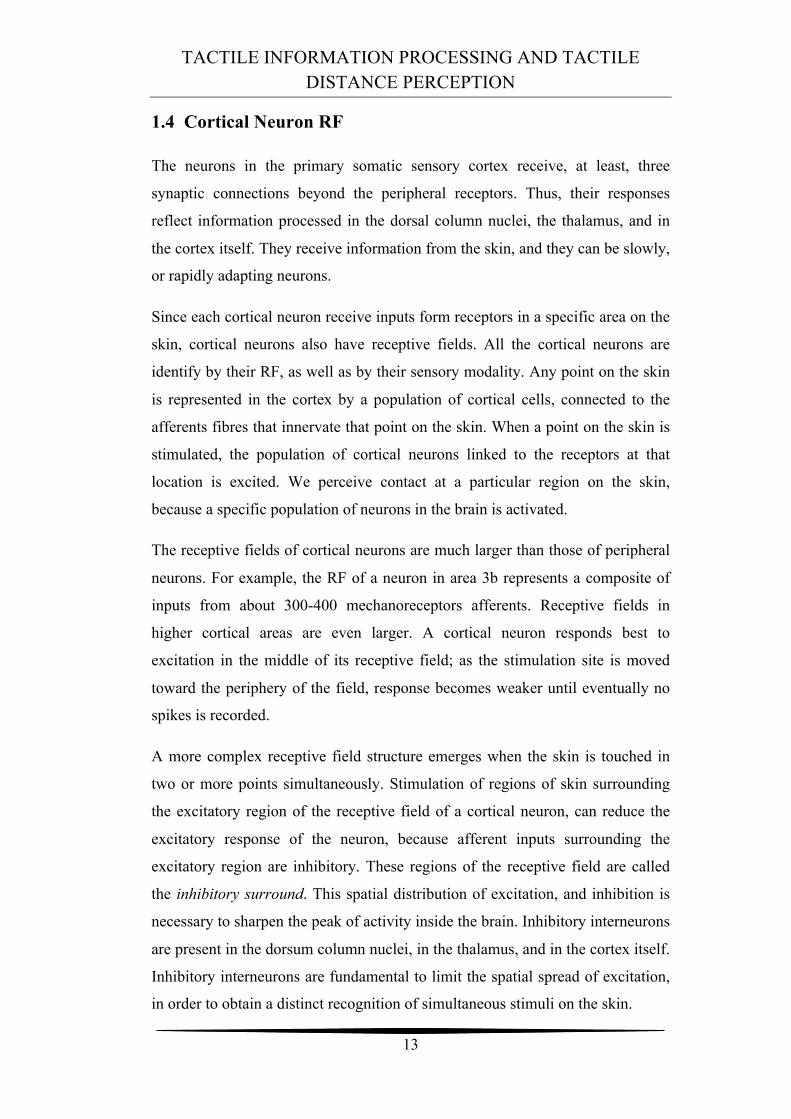
A more complex receptive field structure emerges when the skin is touched in
two or more points simultaneously. Stimulation of regions of skin surrounding
the excitatory region of the receptive field of a cortical neuron, can reduce the
excitatory response of the neuron, because afferent inputs surrounding the
excitatory region are inhibitory. These regions of the receptive field are called
the inhibitory surround. This spatial distribution of excitation, and inhibition is
necessary to sharpen the peak of activity inside the brain. Inhibitory interneurons
are present in the dorsum column nuclei, in the thalamus, and in the cortex itself.
Inhibitory interneurons are fundamental to limit the spatial spread of excitation,
in order to obtain a distinct recognition of simultaneous stimuli on the skin.
TACTILE INFORMATION PROCESSING AND TACTILE DISTANCE PERCEPTION
14
Figure 1. 6 Example of Surround Inhibition.
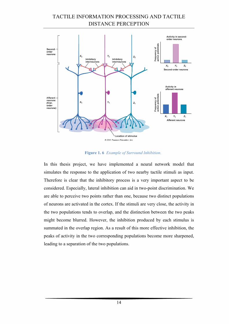
In this thesis project, we have implemented a neural network model that
simulates the response to the application of two nearby tactile stimuli as input.
Therefore is clear that the inhibitory process is a very important aspect to be
considered. Especially, lateral inhibition can aid in two-point discrimination. We
are able to perceive two points rather than one, because two distinct populations
of neurons are activated in the cortex. If the stimuli are very close, the activity in
the two populations tends to overlap, and the distinction between the two peaks
might become blurred. However, the inhibition produced by each stimulus is
summated in the overlap region. As a result of this more effective inhibition, the
peaks of activity in the two corresponding populations become more sharpened,
leading to a separation of the two populations.
TACTILE INFORMATION PROCESSING AND TACTILE DISTANCE PERCEPTION
15
Figure 1. 7 Stimulation of two adjacent points. Lateral Inhibitory networks suppress
excitation of the neurons between the points, sharpening the central focus, and
preserving the spatial clarity of the original stimulus (solid line).
1.5 Tactile Illusion: Weber’s Illusion
In 1834 E. H. Weber described a tactile illusion. Two points kept equidistant
moved over the body surface are felt to converge or diverge. The two points are
perceived as converging, when passing from a high resolution region (hand) to a
less sensitivity region (arm), and are perceived as diverging when passing from a
low-resolution region to a highest one. This means that the same distance
between the two stimulated points is perceived in different way on different
body regions.
A possible explanation of this illusion may be found in the structure (size) of the
RF along the whole body, and also in the variance of receptor density on the skin
surface.
The size of the RFs, in a particular region of skin, establishes the capacity to
determine whether one or more points are stimulated. If two points within the
same receptive field are stimulated, the neuron will signal only one detection.
But if the points are located in the receptive field of two different nerve fibres,
TACTILE INFORMATION PROCESSING AND TACTILE DISTANCE PERCEPTION
16
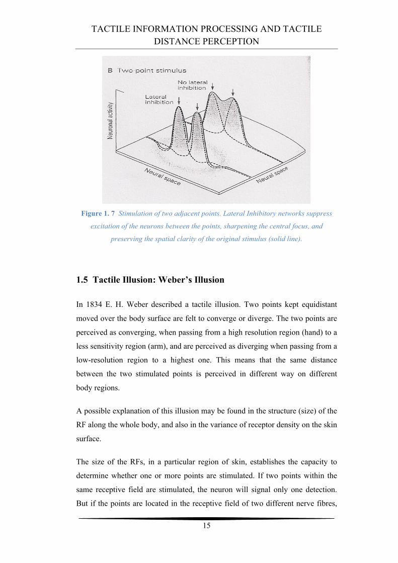
then information about both points of stimulation will be signalled. The contrast
between active, and inactive fibre, seems to be fundamental for resolving spatial
details, or to evaluate the distance between two points. Spatial resolution on
various region of the skin can be quantified in humans by measuring their ability
to perceive a pair of nearby stimuli as two different entities. The minimum
distance between two detectable stimuli is called two point discrimination
threshold.
Figure 1. 8 Two Point Discrimination Threshold along the body.
These variations are correlated with the RF dimension and with the innervation
density of mechanoreceptors on the skin surface.
TACTILE INFORMATION PROCESSING AND TACTILE DISTANCE PERCEPTION
17
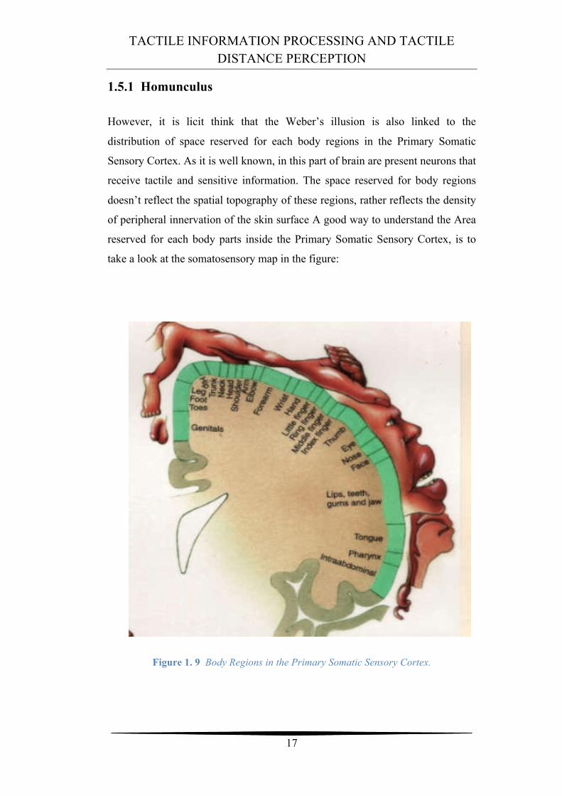
1.5.1 Homunculus
However, it is licit think that the Weber’s illusion is also linked to the
distribution of space reserved for each body regions in the Primary Somatic
Sensory Cortex. As it is well known, in this part of brain are present neurons that
receive tactile and sensitive information. The space reserved for body regions
doesn’t reflect the spatial topography of these regions, rather reflects the density
of peripheral innervation of the skin surface A good way to understand the Area
reserved for each body parts inside the Primary Somatic Sensory Cortex, is to
take a look at the somatosensory map in the figure:
Figure 1. 9 Body Regions in the Primary Somatic Sensory Cortex.
TACTILE INFORMATION PROCESSING AND TACTILE DISTANCE PERCEPTION
18
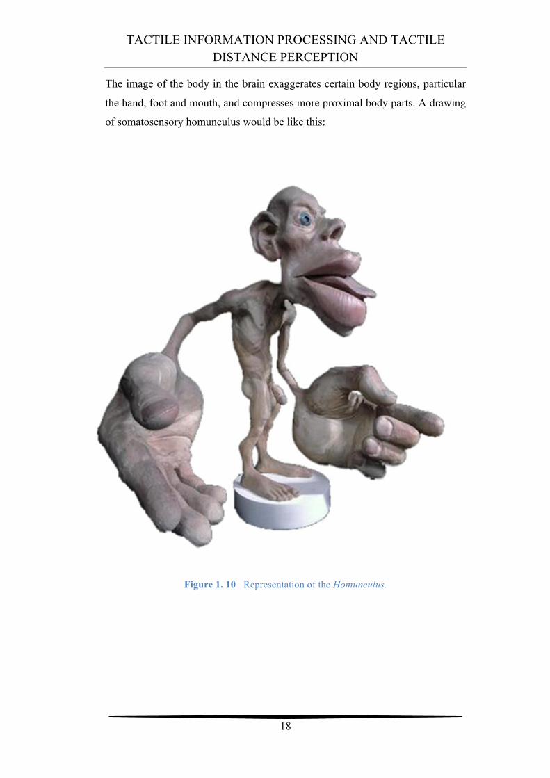
The image of the body in the brain exaggerates certain body regions, particular
the hand, foot and mouth, and compresses more proximal body parts. A drawing
of somatosensory homunculus would be like this:
Figure 1. 10 Representation of the Homunculus.
TACTILE INFORMATION PROCESSING AND TACTILE DISTANCE PERCEPTION
19
The reason for the bizarre, distorted appearance of the homunculus is that the
amount of cerebral tissue, or cortex, devoted to a given body region is
proportional to how richly innervated and sensitive is it, not to its size. In fact,
the map represents the innervation density of the skin rather than its total surface
area. In humans, a lot of cortical columns receive input from the hands,
especially from fingers. Similarly, a large number of cortical neurons receive
input from the foot and the face. The proximal portions of the limbs and trunk,
are much less densely innervated; so, fewer cortical neurons receive inputs from
these regions.
It has to be considered that the somatotopic maps are not fixed, but can change
by experience. The details of the map vary from subject to subject. A tennis
player will develop a larger proportion of cortical neurons devoted to the arm
than a pianist, who needs to increase sensitivity on different fingers.
An important consequence of the magnification of the hands representation in
the cortex, is that the sizes of individual peripheral receptive fields on the hand
cover a much smaller area of skin than receptive fields on the arm, which are
smaller than receptive fields on the trunk. This is a very important aspect linked
to the different resolution on different body parts. So, it is clear that the Weber’s
Illusion is associated with the concept of different resolution along the whole
body.
1.5.2 Magnification concept
To a better understanding about the magnification effect mentioned before, I
suggest to have a look at this article [ “Magnification, Receptive-Field Area, and
Hypercolumn Size in Areas 3b and 1 of Somatosensory Cortex in Owl Monkeys”
MRIGANKA SUR, MICHAEL M. MERZENICH, AND JON H. KAAS ], in
which several features in cortical area 3b, and 1, of somatosensory cortex in
monkeys, were quantitatively studied. In particular, some experiments
performed in that work led to a quantification of the magnification of body
regions inside the primary cortex.
TACTILE INFORMATION PROCESSING AND TACTILE DISTANCE PERCEPTION
20
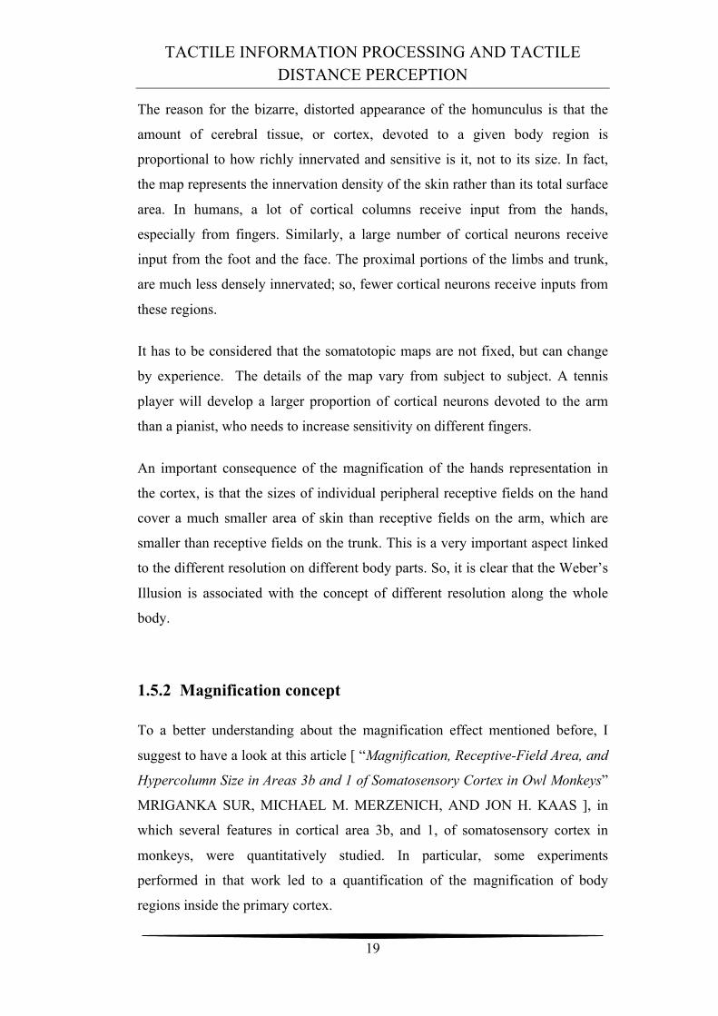
The overall magnification curve is illustrated below:
Figure 1. 11 Recorded Magnification for different body regions in the MRIGANKA’s
experiment.
Cortical Magnification varies greatly across different body regions. For example,
the glabrous hand, or foot representation, occupies nearly 100 times more
cortical tissue per unit body surface area than the trunk, or arm representations in
both areas 3b, and 1. Even if these data comes from monkey, they can be also
used to study the magnification in the human body, as there are several evidence
about the similarity between the monkey’s cortex, and human’s cortex. This
means that if we are going to consider a square surface area of 5x5 cm on the
hand, and 10x10 cm on the arm, the equivalent regions in the primary somatic
sensory cortex can be obtained with this simple equation:
Skin × Magnification = Cortex
TACTILE INFORMATION PROCESSING AND TACTILE DISTANCE PERCEPTION
21
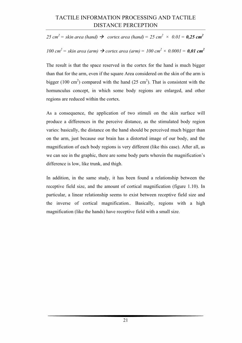
25 cm2 = skin area (hand) à cortex area (hand) = 25 cm2 × 0.01 = 0,25 cm2
100 cm2 = skin area (arm) à cortex area (arm) = 100 cm2 × 0.0001 = 0,01 cm2
The result is that the space reserved in the cortex for the hand is much bigger
than that for the arm, even if the square Area considered on the skin of the arm is
bigger (100 cm2) compared with the hand (25 cm2). That is consistent with the
homunculus concept, in which some body regions are enlarged, and other
regions are reduced within the cortex.
As a consequence, the application of two stimuli on the skin surface will
produce a differences in the perceive distance, as the stimulated body region
varies: basically, the distance on the hand should be perceived much bigger than
on the arm, just because our brain has a distorted image of our body, and the
magnification of each body regions is very different (like this case). After all, as
we can see in the graphic, there are some body parts wherein the magnification’s
difference is low, like trunk, and thigh.
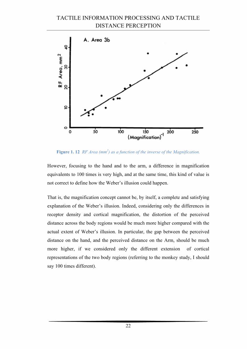
In addition, in the same study, it has been found a relationship between the
receptive field size, and the amount of cortical magnification (figure 1.10). In
particular, a linear relationship seems to exist between receptive field size and
the inverse of cortical magnification.. Basically, regions with a high
magnification (like the hands) have receptive field with a small size.
TACTILE INFORMATION PROCESSING AND TACTILE DISTANCE PERCEPTION
22
Figure 1. 12 RF Area (mm2) as a function of the inverse of the Magnification.
However, focusing to the hand and to the arm, a difference in magnification
equivalents to 100 times is very high, and at the same time, this kind of value is
not correct to define how the Weber’s illusion could happen.
That is, the magnification concept cannot be, by itself, a complete and satisfying
explanation of the Weber’s illusion. Indeed, considering only the differences in
receptor density and cortical magnification, the distortion of the perceived
distance across the body regions would be much more higher compared with the
actual extent of Weber’s illusion. In particular, the gap between the perceived
distance on the hand, and the perceived distance on the Arm, should be much
more higher, if we considered only the different extension of cortical
representations of the two body regions (referring to the monkey study, I should
say 100 times different).
TACTILE INFORMATION PROCESSING AND TACTILE DISTANCE PERCEPTION
23
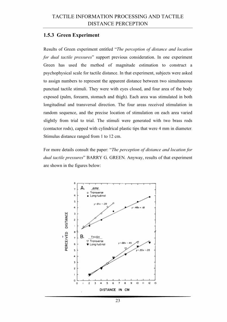
1.5.3 Green Experiment
Results of Green experiment entitled “The perception of distance and location
for dual tactile pressures” support previous consideration. In one experiment
Green has used the method of magnitude estimation to construct a
psychophysical scale for tactile distance. In that experiment, subjects were asked
to assign numbers to represent the apparent distance between two simultaneous
punctual tactile stimuli. They were with eyes closed, and four area of the body
exposed (palm, forearm, stomach and thigh). Each area was stimulated in both
longitudinal and transversal direction. The four areas received stimulation in
random sequence, and the precise location of stimulation on each area varied
slightly from trial to trial. The stimuli were generated with two brass rods
(contactor rods), capped with cylindrical plastic tips that were 4 mm in diameter.
Stimulus distance ranged from 1 to 12 cm.
For more details consult the paper: “The perception of distance and location for
dual tactile pressures” BARRY G. GREEN. Anyway, results of that experiment
are shown in the figures below:
TACTILE INFORMATION PROCESSING AND TACTILE DISTANCE PERCEPTION
24
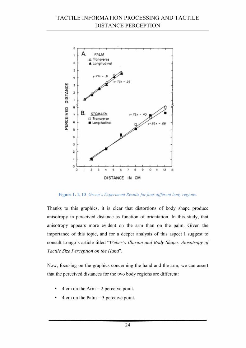
Figure 1. 1. 13 Green’s Experiment Results for four different body regions.
Thanks to this graphics, it is clear that distortions of body shape produce
anisotropy in perceived distance as function of orientation. In this study, that
anisotropy appears more evident on the arm than on the palm. Given the
importance of this topic, and for a deeper analysis of this aspect I suggest to
consult Longo’s article titled “Weber’s Illusion and Body Shape: Anisotropy of
Tactile Size Perception on the Hand”.
Now, focusing on the graphics concerning the hand and the arm, we can assert
that the perceived distances for the two body regions are different:
• 4 cm on the Arm = 2 perceive point.
• 4 cm on the Palm = 3 perceive point.
TACTILE INFORMATION PROCESSING AND TACTILE DISTANCE PERCEPTION
25
These results verify the existence of tactile spatial distortions that were first
reported by Weber. But this difference is not as high as the difference in the
cortical magnification of the two body regions. Considering only differences in
cortical magnification, the difference between the two perceived distances
should be much bigger.
So, we can confirm that the magnification plays a key role in the Weber’s
Illusion, because sets a distortion in terms of extension of cortical representation
inside the primary cortex, but for sure is not the unique process. We hypothesize
that there must be present other processing of tactile information that performs a
sort of “rescaling”; this rescaling process, may act by decreasing the huge initial
gap due to the different cortical magnification, still providing only a partial
compensation (the final result is the Weber’s illusion). The neural mechanisms
underlying the Weber’s illusion are still largely unknown.
1.6 The neural network and the simplifying assumptions
In this thesis, I developed a neural network model that aspires to contribute to
clarify the neural mechanisms producing Weber’s illusion. Some hypotheses
have been considered in model implementation; the main hypothesis is that the
process of perceived distance involves two layers in the brain. The first one may
correspond to the Primary Somatic Sensory Cortex, which receives inputs from
the skin surface, wherein we can observe the effect of “Cortical Magnification” .
The second layer, linked with feed-forward synapses to the first one, is a higher-
level area: it enables to implement a sort of rescaling about the perceived
distance, that partially compensates the huge effect resulting from cortical
magnification. See the scheme below:
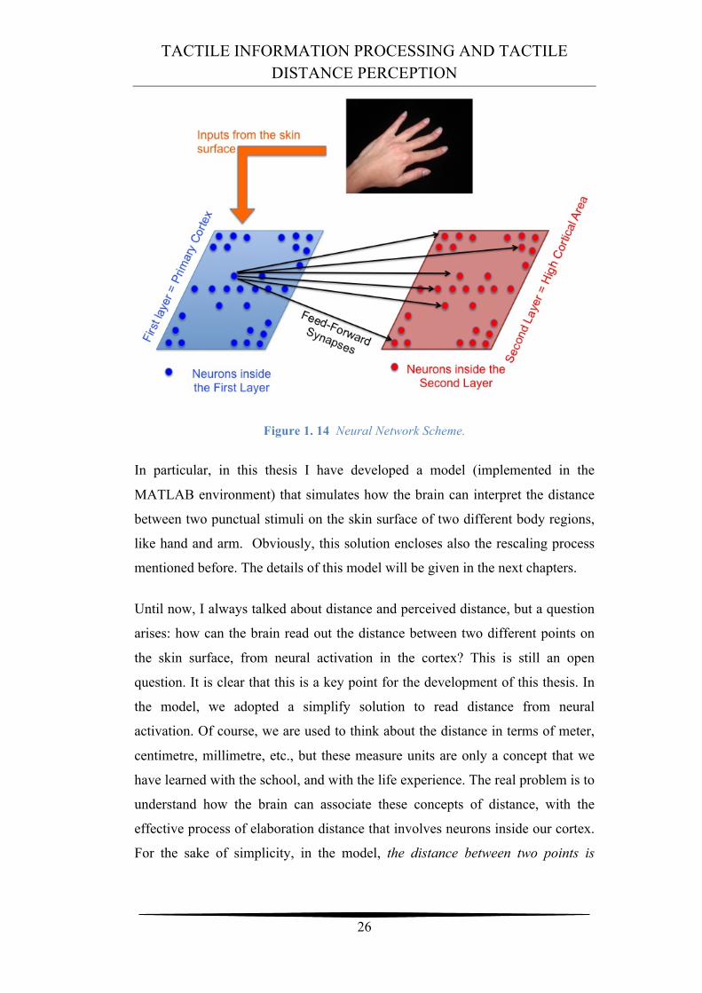
TACTILE INFORMATION PROCESSING AND TACTILE DISTANCE PERCEPTION
26
Figure 1. 14 Neural Network Scheme.
In particular, in this thesis I have developed a model (implemented in the
MATLAB environment) that simulates how the brain can interpret the distance
between two punctual stimuli on the skin surface of two different body regions,
like hand and arm. Obviously, this solution encloses also the rescaling process
mentioned before. The details of this model will be given in the next chapters.
Until now, I always talked about distance and perceived distance, but a question
arises: how can the brain read out the distance between two different points on
the skin surface, from neural activation in the cortex? This is still an open
question. It is clear that this is a key point for the development of this thesis. In
the model, we adopted a simplify solution to read distance from neural
activation. Of course, we are used to think about the distance in terms of meter,
centimetre, millimetre, etc., but these measure units are only a concept that we
have learned with the school, and with the life experience. The real problem is to
understand how the brain can associate these concepts of distance, with the
effective process of elaboration distance that involves neurons inside our cortex.
For the sake of simplicity, in the model, the distance between two points is
TACTILE INFORMATION PROCESSING AND TACTILE DISTANCE PERCEPTION
27
interpreted in terms of the number of inactivated neurons between two excited
populations of cortical neurons (activated by two punctual tactile stimuli).
This chapter is conceived as an introduction, entering the main problem faced by
this thesis work. In the next Chapters, I will describe the mathematical model
used to simulate Weber’s illusion.
Chapter 2
MATHEMATICAL MODEL
2.1 Qualitative description of the model
2.1.1 The two main layers
The model aims to reproduce the main steps inside the cortex leading to the
perception of distance between a pair of stimuli applied on the skin surface. To
this end, two layers of artificial neurons (that may correspond to two different
levels of somatosensory processing in the cerebral cortex) have been used.
The main idea about this model is that the first layer could represent skin
receptors plus primary somatosensory cortex neurons, and it may synthesize the
property receptor density-cortical magnification of a skin region. An external
tactile input directly stimulates this layer.
Suppose this first layer consists of 41 x 41 units (simulating cortical neurons),
corresponding to a skin region of K x K cm (at the moment it does not matter the
dimension of the represented skin region. This will be specified later). Each unit
on this layer has a Receptive Field (RF) covering a specific portion on the skin
surface. Since there are 41 neurons on each side of the matrix, the centres of the
RFs are arranged at a distance of:
K cm / 41 neurons
A punctual stimulus, applied in a certain position, activates a “bubble” of
neurons on the first layer, in particular all the neurons whose RFs cover that
position.
The second layer may represent higher cortical area involved in tactile distance
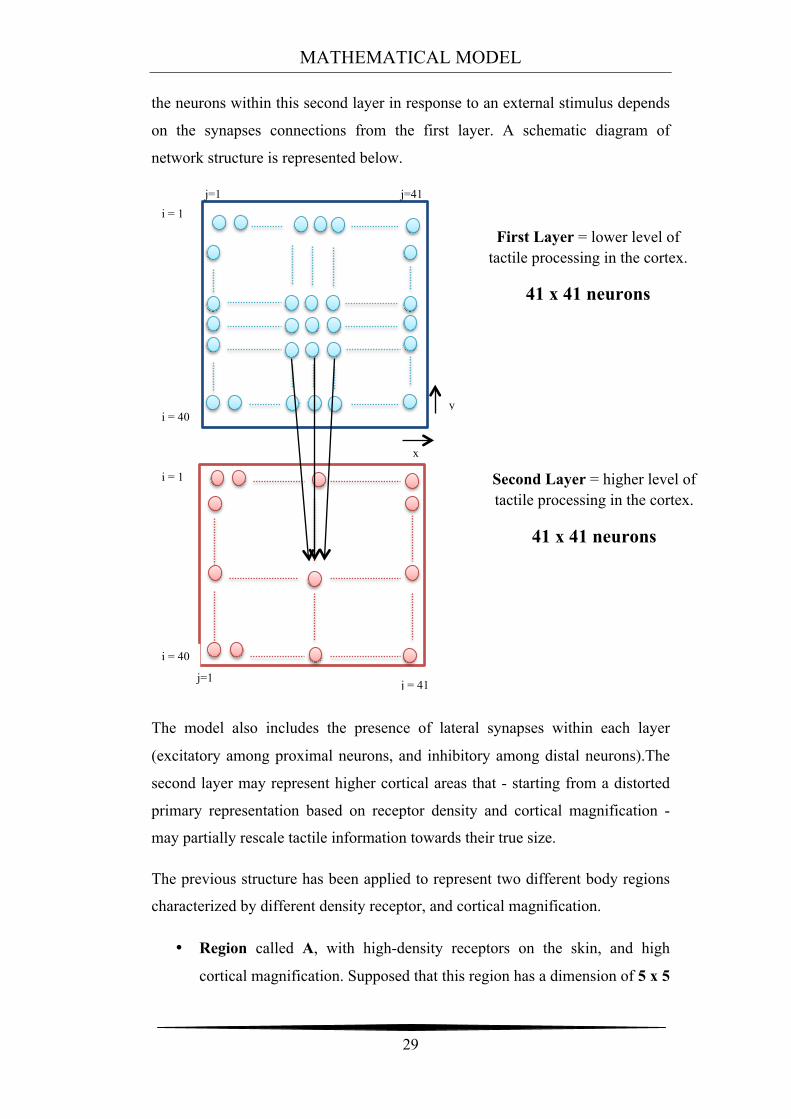
perception, receiving synapses from the first layer. I have assumed that this layer
have the same number of units as the first layer (41 x 41 neurons). Activation of
MATHEMATICAL MODEL
29
the neurons within this second layer in response to an external stimulus depends
on the synapses connections from the first layer. A schematic diagram of
network structure is represented below.
The model also includes the presence of lateral synapses within each layer
(excitatory among proximal neurons, and inhibitory among distal neurons).The
second layer may represent higher cortical areas that - starting from a distorted
primary representation based on receptor density and cortical magnification -
may partially rescale tactile information towards their true size.
The previous structure has been applied to represent two different body regions
characterized by different density receptor, and cortical magnification.
• Region called A, with high-density receptors on the skin, and high
cortical magnification. Supposed that this region has a dimension of 5 x 5
i = 1
i = 40
x
y
j = 41
j=1 j=41
First Layer = lower level of tactile processing in the cortex.
41 x 41 neurons
Second Layer = higher level of tactile processing in the cortex.
41 x 41 neurons
i = 1
i = 40
j=1
MATHEMATICAL MODEL
30
cm on the skin surface, and it is mapped by a matrix of 41 x 41 neurons
in the cortex. In addition, each neuron has small RF size.
• Region called B, with low-density receptors on skin, and low cortical
magnification. Supposed that this region has a dimension of 10 x 10 cm
on the skin surface, and it is mapped by a matrix of 41 x 41 neurons in
the cortex.. In addition, neurons in this area have large RF size.
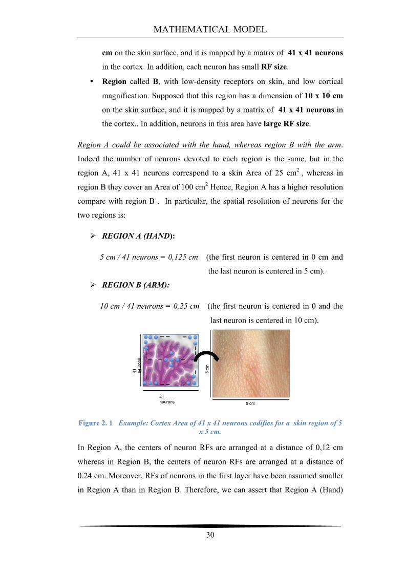
Region A could be associated with the hand, whereas region B with the arm.
Indeed the number of neurons devoted to each region is the same, but in the
region A, 41 x 41 neurons correspond to a skin Area of 25 cm2 , whereas in
region B they cover an Area of 100 cm2 Hence, Region A has a higher resolution
compare with region B . In particular, the spatial resolution of neurons for the
two regions is:
Ø REGION A (HAND):
5 cm / 41 neurons = 0,125 cm (the first neuron is centered in 0 cm and
the last neuron is centered in 5 cm).
Ø REGION B (ARM):
10 cm / 41 neurons = 0,25 cm (the first neuron is centered in 0 and the
last neuron is centered in 10 cm).
Figure 2. 1 Example: Cortex Area of 41 x 41 neurons codifies for a skin region of 5 x 5 cm.
In Region A, the centers of neuron RFs are arranged at a distance of 0,12 cm
whereas in Region B, the centers of neuron RFs are arranged at a distance of
0.24 cm. Moreover, RFs of neurons in the first layer have been assumed smaller
in Region A than in Region B. Therefore, we can assert that Region A (Hand)
MATHEMATICAL MODEL
31
has higher acuity in discriminating the presence of two nearby stimuli. Instead
the arm acuity will be lower.
To summarize, the first layer of this model accounts for cortical magnification
that occurs in the primary somatosensory cortex: indeed, in this first layer,
Region A is represented by a higher number of neurons having smaller RF,
whereas Region B is represented by a lower number of neurons having larger
RFs. That is, this layer gives rise to a strong distorted representation. The second
layer has been included to restore, at least, partially a more truthful
representation
2.1.2 Application of two punctual stimuli : effects within the first
layer
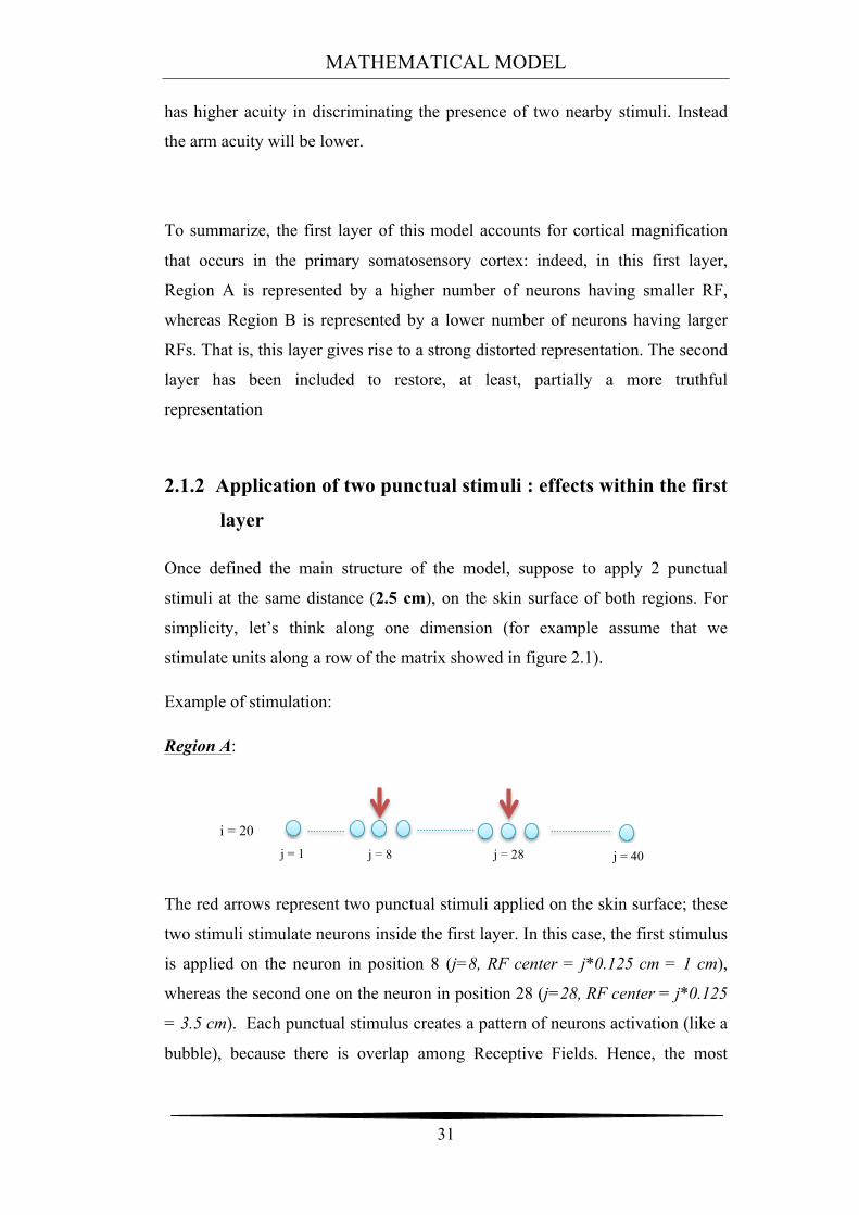
Once defined the main structure of the model, suppose to apply 2 punctual
stimuli at the same distance (2.5 cm), on the skin surface of both regions. For
simplicity, let’s think along one dimension (for example assume that we
stimulate units along a row of the matrix showed in figure 2.1).
Example of stimulation:
Region A:
The red arrows represent two punctual stimuli applied on the skin surface; these
two stimuli stimulate neurons inside the first layer. In this case, the first stimulus
is applied on the neuron in position 8 (j=8, RF center = j*0.125 cm = 1 cm),
whereas the second one on the neuron in position 28 (j=28, RF center = j*0.125
= 3.5 cm). Each punctual stimulus creates a pattern of neurons activation (like a
bubble), because there is overlap among Receptive Fields. Hence, the most
i = 20 j = 1 j = 8 j = 28 j = 40
MATHEMATICAL MODEL
32
excited neurons will be the eighth and the twenty-eighth, but also their neighbors
will be activated, even if with a less strength.
Therefore, the pattern of neuron activation along the 20th lines of the matrix (first
layer), should be like this:
Figure 2. 2 Peaks of activation along the 20th lines of the neurons matrix (Area 1, HAND).
Notice the distance between two peaks: 20 neurons.
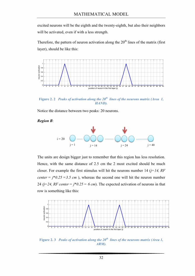
Region B:
The units are design bigger just to remember that this region has less resolution.
Hence, with the same distance of 2.5 cm the 2 most excited should be much
closer. For example the first stimulus will hit the neurons number 14 (j=14, RF
center = j*0.25 =3.5 cm ), whereas the second one will hit the neuron number
24 (j=24, RF center = j*0.25 = 6 cm). The expected activation of neurons in that
row is something like this:
Figure 2. 3 Peaks of activation along the 20th lines of the neurons matrix (Area 1, ARM).
1 2 3 4 5 6 7 8 9 10 11 12 13 14 15 16 17 18 19 20 21 22 23 24 25 26 27 28 29 30 31 32 33 34 35 36 37 38 39 400
0.2
0.4
0.6
0.8
1
position of neuron in the first layer (j)
neur
on a
ctiv
atio
n
1 2 3 4 5 6 7 8 9 10 11 12 13 14 15 16 17 18 19 20 21 22 23 24 25 26 27 28 29 30 31 32 33 34 35 36 37 38 39 400
0.2
0.4
0.6
0.8
1
position of neuron in the first layer (j)
neur
on a
ctiv
atio
n
i = 20
j = 40 j = 24 j = 14 j = 1
MATHEMATICAL MODEL
33
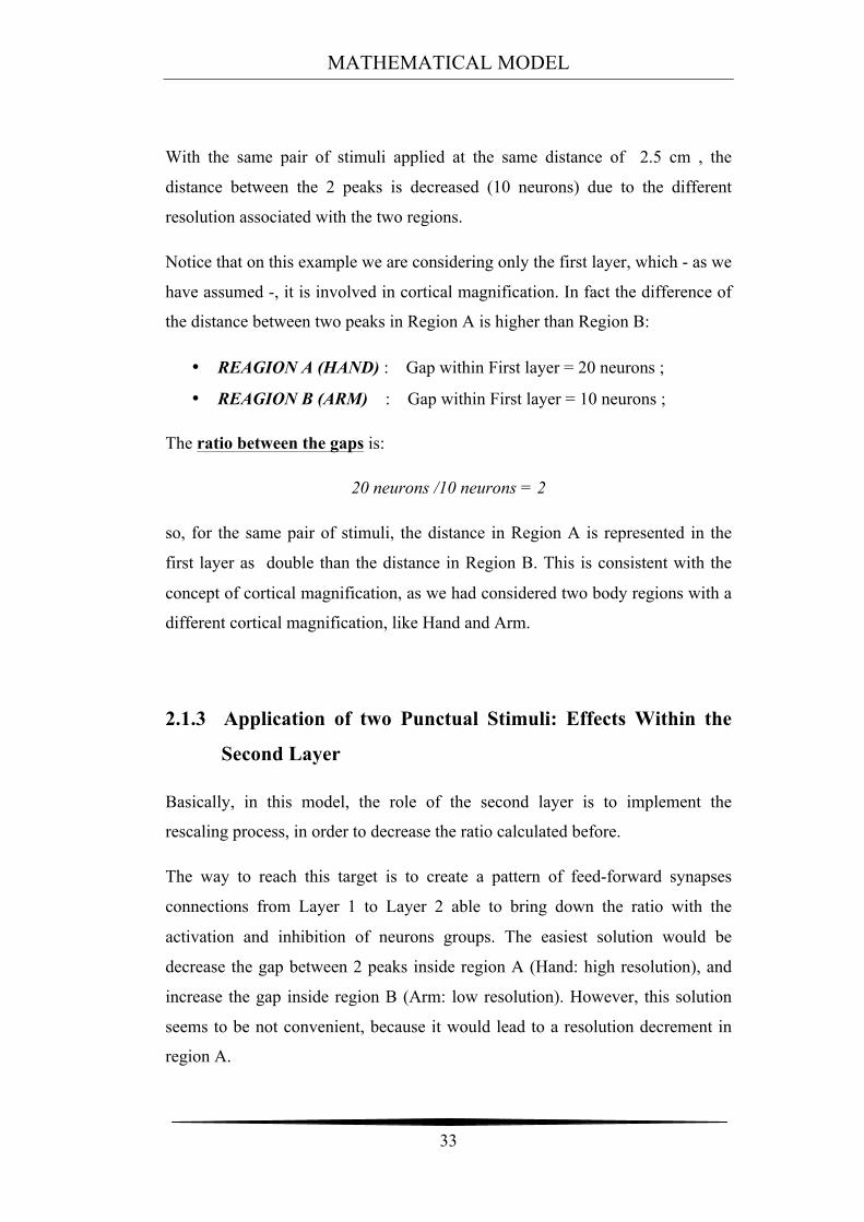
With the same pair of stimuli applied at the same distance of 2.5 cm , the
distance between the 2 peaks is decreased (10 neurons) due to the different
resolution associated with the two regions.
Notice that on this example we are considering only the first layer, which - as we
have assumed -, it is involved in cortical magnification. In fact the difference of
the distance between two peaks in Region A is higher than Region B:
• REAGION A (HAND) : Gap within First layer = 20 neurons ;
• REAGION B (ARM) : Gap within First layer = 10 neurons ;
The ratio between the gaps is:
20 neurons /10 neurons = 2
so, for the same pair of stimuli, the distance in Region A is represented in the
first layer as double than the distance in Region B. This is consistent with the
concept of cortical magnification, as we had considered two body regions with a
different cortical magnification, like Hand and Arm.
2.1.3 Application of two Punctual Stimuli: Effects Within the
Second Layer
Basically, in this model, the role of the second layer is to implement the
rescaling process, in order to decrease the ratio calculated before.
The way to reach this target is to create a pattern of feed-forward synapses
connections from Layer 1 to Layer 2 able to bring down the ratio with the
activation and inhibition of neurons groups. The easiest solution would be
decrease the gap between 2 peaks inside region A (Hand: high resolution), and
increase the gap inside region B (Arm: low resolution). However, this solution
seems to be not convenient, because it would lead to a resolution decrement in
region A.
MATHEMATICAL MODEL
34
Therefore, it should be better a different implementation; as long as we want to
maintain the high resolution of the region A (Hand) , it is much more convenient
to work only by incrementing the resolution of the region B (Arm).
Hence, I have hypothesized that the brain implements the rescaling process by
increasing the resolution of the lowest resolution region (region B in this case).
At the same time, the high resolution of the region A presents in the first layer,
will be kept also in the second layer too.
It is clear that to implement such kind of process, the synapses within the
network concerning Region A will be different (in terms of parameters) from
the network concerning Region B.
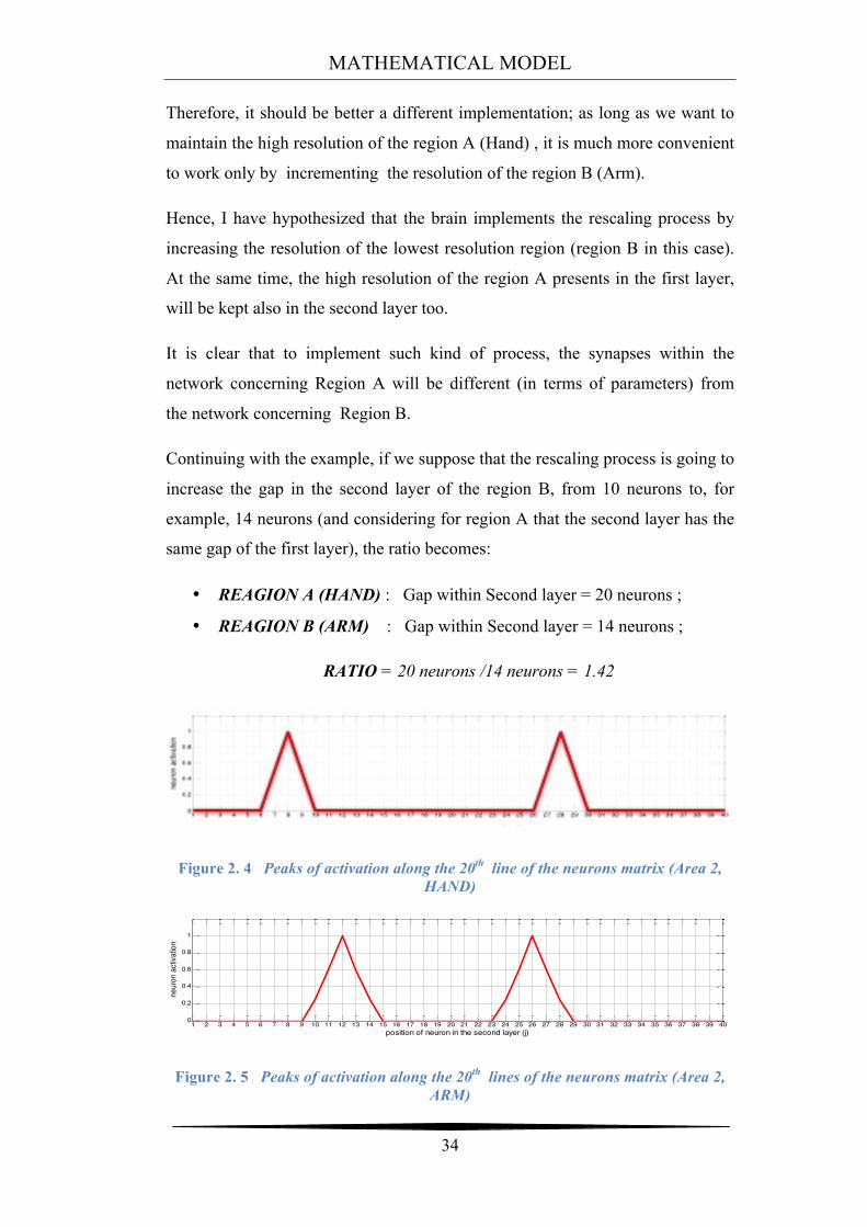
Continuing with the example, if we suppose that the rescaling process is going to
increase the gap in the second layer of the region B, from 10 neurons to, for
example, 14 neurons (and considering for region A that the second layer has the
same gap of the first layer), the ratio becomes:
• REAGION A (HAND) : Gap within Second layer = 20 neurons ;
• REAGION B (ARM) : Gap within Second layer = 14 neurons ;
RATIO = 20 neurons /14 neurons = 1.42
Figure 2. 4 Peaks of activation along the 20th line of the neurons matrix (Area 2, HAND)
Figure 2. 5 Peaks of activation along the 20th lines of the neurons matrix (Area 2, ARM)
1 2 3 4 5 6 7 8 9 10 11 12 13 14 15 16 17 18 19 20 21 22 23 24 25 26 27 28 29 30 31 32 33 34 35 36 37 38 39 400
0.2
0.4
0.6
0.8
1
position of neuron in the second layer (j)
neur
on a
ctiva
tion
MATHEMATICAL MODEL
35
Therefore, the illusion is still present, but now, on the second layer, the
perceived distance is more similar across the two regions, with respect to what
occurs in the first layer. That is, representation in the second layer is more
truthful, since actually the distance applied externally is the same. That is, the
second layer partially rescales the distortion occurring in the first layer, by
reducing the difference in the perceived distance. So, in this model, the
fundamental hypothesize is that the second layer (higher cortical level) of each
body regions plays a key role in the perception of distance about two stimuli.
2.2 Mathematical description of the network
Since the networks representing Region A and Region B, has the same structure,
only the equations for the Hand region will be presented. However, the two
networks differ for the parameter values of some synapses. Hence, after
description of network structure, I will emphasize the difference in parameter
values between the two Regions.
The superscripts f, s will denote quantities concerning the first layer (Area 1) and
the second layer (Area 2) respectively. The superscripts H and A will indicate
the Hand (Region A) and the Arm (Region B). Finally the subscripts ij, hk will
represent the spatial position of an individual neuron.
Each layer can be thought as a matrix of neurons. In the model, each layer is
composed by N x N neurons with N = 41. The dimension of this matrix is the
same for both regions. For Region A, this Area (matrix) corresponds to a skin
region on the hand of 5 x 5 cm. Instead in Region B, this Area (matrix) is
relative to a skin region on the arm of 10 x 10 cm.
To replicate the different resolution, RF’s centers are arranged at a distance of
0.125 cm on the Hand, and 0.25 cm on the Arm,.
In the following, I will denote with xi and yi the center of the RF of a generic
neuron ij. By considering a reference frame rigidly connected with the Hand, we
can write:
MATHEMATICAL MODEL
36
xi = -2.625 cm + i ⋅ 0.125 cm ( i = 1, 2, …. , N) (2.1)
yj = -2.625 cm +j ⋅ 0.125 cm (j = 1, 2, …. , N) (2.2)
The same formula can be used for the Arm:
xi = -5.25 cm + i ⋅ 0.25 cm ( i = 1, 2, …. , N) (2.3)
yj = -5.25 cm + j ⋅.0.25cm (j = 1, 2, …. , N) (2.4)
Hereinafter, the RF will be denoted with the symbol Φ (receptive field). The RF
of the cortical neurons in “Area 1” is described with a Gaussian Function.
Therefore, for a neuron ij in “Area 1” the following equation holds:
!ijf ,H (x, y) =!0
f ,H "exp #(x # xi
f ,H )2 + (y# yjf ,H )2
2 " (!!f ,H )2
$
%&&
'
())
(2.5)
where xi, yi is the centre of the RF (on the skin), x and y are the spatial
coordinates (still relative to the skin surface), and !0s and !!
s , represent the
amplitude and the standard deviation of the Gaussian Function (three standard
deviation approximately cover the overall RF). According to the equation, an
external stimulus applied at the position (x,y) excites not only the neuron centred
in that position, but also the proximal neurons with RFs covering that point.
2.2.1 First layer of neurons (Area 1)
The total input received by a generic neuron ij in “Area 1” is the sum of two
contributes:
• The contribution due to the external stimulus applied on the skin (called
!ij (t) ).
• The contribution due to the lateral synapses, linking the neuron with
other neurons within the same “Area 1” (called !ij (t) ).
MATHEMATICAL MODEL
37
The input that reaches the neuron ij in presence of an external stimulus, is
calculated as the product of the strength of the stimulus and the receptive field,
according to this equation:
!ijf ,H (t) = !ij
f ,H
y"
x" (x, y) # I f ,H (x, y, t)dxdy
! "ijf ,H
y#
x# (x, y) $ I f ,H (x, y, t)%x%y (2.6)
Where I f ,H is the external stimulus applied on the skin (Hand or Arm) at the
coordinates (x,y) at the time t. The right side of the equation (num. 2.6) means
that the integral is computed with the histogram rule !x = !y = 0.0312cm .
In this model the external stimulus is reproduced as a two dimensional Gaussian
Function (like a circular point):
I f ,H (x, y, t) =
0, t < t0
I0f ,H !exp "
(x " x0f ,H )2 + (y" y0
f ,H )2
2 ! (! If )2
#
$%
&
'( , t > t0
)
*++
,++
(2.7)
Where t0 is the instant of stimulus application, (x0, y0) is the central point of the
stimulus, and I0f ,H and ! I
f , are the amplitude, and the standard deviation of the
stimulus, respectively. I have used a small standard deviation to simulate a
punctual external stimulus (see Table).
In this model the application of 2 external stimuli is simulated, applied at the
same time in 2 different positions. Hence, the application of 2 stimuli is
represented by the following equation:
MATHEMATICAL MODEL
38
I f ,H (x, y, t) =
0, t < t0
I1f ,H !exp "
(x " x1f ,H )2 + (y" y1
f ,H )2
2 ! (! I1f )2
#
$%
&
'( + I2
s !exp "(x " x2
f ,H )2 + (y" y2f ,H )2
2 ! (! I 2f )2
#
$%
&
'( , t > t0
)
*++
,++
(2.8)
The input that a cortical neuron ij receives from other neurons within the same
Area via lateral synapses, is computed as:
!ijl,H (t) = Lij,hk
l,H
k=1
Nl
!h=1
Nl
! ""hkl,H (t), l = f , s.
(2.9)
!hkl,H (t) represents the activity of the neuron in position (h,k) inside “Area 1”,
and it is a variable state. Lij,hkl,H is the strength of the synaptic connection from the
pre-synaptic neuron (h,k), to the postsynaptic neuron at the position (i,j). These
synapses are symmetrical and are organized as a Mexican Hat function
(excitation among nearby neurons, and inhibition among distant neurons). The
equation implementing Lateral Synapses is valid for the first layer, as well as for
the second layer:
!!",!!!,! =
!!"!,! ∙ exp −
(!!!,!!!!
!,!)!!(!!!,!!!!
!,!)!
!∙ !!!"!,! !
−!!"!,! ∙ exp −
(!!!,!!!!
!,!)!!(!!!,!!!!
!,!)!
!∙ !!!"!,! ! , !" ≠ ℎ!
0, !" = ℎ!
(2.10)
l = f , s.
xi and yj represent the position of the post-synaptic neuron within the “Area 1”
and xh, yk represent the position of the presynaptic neuron within Area1. Lexl,H
and !!!"!,! define the Excitatory Gaussian function, whereas parameters Lin
l,H and
!!!"!,! the Inhibitory one. To implement a correct Mexican Hat function, some
conditions have to be satisfied:
!!"!,! > !!"
!,! ! = !, !. (2.11)
MATHEMATICAL MODEL
39
!!"#!,! < !!"#
!,! ! = !, ! (2.12)
The null term in equation (num. 2.10), avoids the auto-excitation.
Finally, the total input, called uijf ,H (t) received by a cortical neuron in “Area 1”
(First Layer) is the sum of the two contributes:
uijf ,H (t) =!ij
f ,H (t)+"ijf ,H (t) . (2.13)
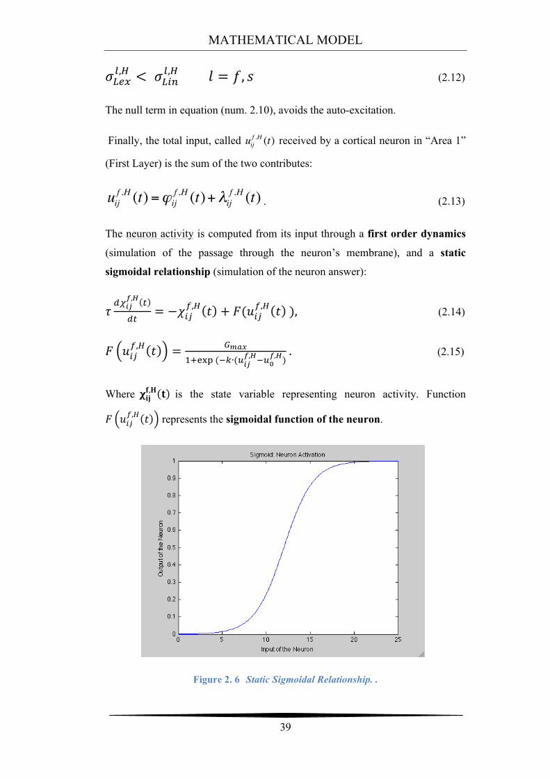
The neuron activity is computed from its input through a first order dynamics
(simulation of the passage through the neuron’s membrane), and a static
sigmoidal relationship (simulation of the neuron answer):
!!!!"
!,! !
!"= −!!"
!,! ! + !(!!"!,! ! ), (2.14)
! !!"!,! ! = !!"#
!!!"# (!!∙(!!"!,!!!!
!,!) . (2.15)
Where !!"!,! ! is the state variable representing neuron activity. Function
! !!"!,! ! represents the sigmoidal function of the neuron.
Figure 2. 6 Static Sigmoidal Relationship. .
MATHEMATICAL MODEL
40
The parameter is the value of the input at the central point (that is the value of
the input at which activity is equal to Gmax/2; is the slope of the sigmoid at
the central point, and is the upper saturation value of the sigmoid, that is
the maximum activity value for a generic neuron. Gmax has been set equal to 1,
so that neuron activity is normalized with respect to its maximum. According to
previous equation (num. 2.15), the activity of a generic neuron inside “Area 1” is
equal to zero until its total input is under a given threshold. ! is the time constant
of the differential equation (num. 2.14).
Differential equation (num. 2.14) is implemented numerically with the Euler’s
method:
!!!!!",! = !!
!",! + ℎ ∙ ! ! , !!!",! , ℎ = !
!. (2.16)
!!!!!",! = !!
!",! + !!∙ −!!
!",! + !!"#
!!!"# (!!∙(!!"!,!!!!
!,!) (2.17)
As long as T is the time length of the simulation, and P is the number of
subdivisions of T, it is clear that h represents the sampling step of the Euler’s
method.
2.2.2 Second layer of neurons (Area 2)
The Second Layer (Area 2) is assumed to be associated with a high cortical
layer. In this model, neurons inside this area, receive inputs from:
• Neurons in “Area 1” via Feed-Forward synapses, having a Mexican Hat
distribution.
• Neurons of the same Area via Lateral Synapses, having a Mexican hat
distribution.
The following equations hold:
(2.18)
u0f
k
Gmax
uijs,H (t) =! ij
s,H (t)+!ijs,H (t)
MATHEMATICAL MODEL
41
! ijs,H (t) = Wij,hk
f ,H
k=1
N f
"h=1
N f
" #!hkf ,H (t),
(2.19)
!hkf ,H (t) represents the activity of the neuron hk in “Area 1”. Wij,hk
f ,H denotes the
feed-forward synaptic strength from the pre-synaptic cortical neuron hk in “Area
1”, to the post-synaptic neuron ij in “Area 2”. These synapses can be described
as follows:
!!",!!!,! = !!"
!,! ∙ exp −(!!!,!!!!
!,!)!!(!!!,!!!!
!,!)!
!∙ !!!"!,! ! +
−!!"!,! ∙ exp −
(!!!,!!!!
!,!)!!(!!!,!!!!
!,!)!
!∙ !!!"!,! !
(2.20)
Where xis,H , yjs,H , represents the position of the ij neuron in “Area 2”, and xh
f ,H ,
ykf ,H , the position of the neuron hk in “Area 1”. Notice that when the coordinates
of these two neurons are equals, the exponential term assumes an unitary value,
and then the synapse connection between these two neurons has the strongest
value.
The activity of a neuron in “Area 2” can be computed from its input with the
same equation as before (num. 2.14):
!!!!"
!,! !
!"= −!!"
!,! ! + ! !!"!,! ! , (2.21)
! !!"!,! ! = !!"#
!!!"# (!!∙(!!"!,!!!!
!,!) . (2.22)
k is the slope of the sigmoid at the central point, is the value of the input at
the central point, and is the gain of the sigmoidal function.
It can be solved by Euler’s method:
!!!!!",! = !!
!",! + ℎ ∙ ! ! , !!!",! ℎ = !
! (2.23)
!!!!!",! = !!
!",! + !!∙ −!!
!",! + !!"#
!!!"# (!!∙(!!"!,!!!!
!,!). (2.24)
u0f
Gmax
MATHEMATICAL MODEL
42
As long as T is the time length of the simulation, and P is the number of
subdivisions of T, it is clear that h represents the sampling step of the Euler’s
method.
2.3 Parameters and their values
External Stimuli
I1f ,H =1.5 I2
f ,H =1.5 ! I1f ,H = 0.1 cm ! I 2
f ,H = 0.1 cm
I1f ,A =1.5 I2
f ,A =1.5 ! I1f ,A = 0.1 cm ! I 2
f ,A = 0.1 cm
Receptive Fields
!0f ,H =1 !!
f ,H = 0.125 cm
!0f ,A =1 !!
f ,A = 0.35 cm
Lateral Synapses in Area 1
Lexf ,H =1 Lin
f ,H = 0.5 ! exf ,H = 2 neurons ! in
f ,H = 8 neurons
Lexf ,A =1 Lin
f ,A = 0.5 ! Lexf ,A = 2 neurons ! Lin
f ,A = 8 neurons
Feed-Forward Synapses
Wexf ,H = 4 Win
f ,H =1 !Wexf ,H =1neurons !Win
f ,H =1.4 neurons
Wexf ,A = 4 Win
f ,A =1 !Wexf ,A =1neurons !Win
f ,A =1.4 neurons
Lateral Synapses in Area 2
Lexs,H = 4.5 Lin
s,H = 2 ! exs,H =1.5 neurons ! in
s,H = 2 neurons
Lexs,A = 4.5 Lin
s,A = 2 ! exs,A =1neurons ! in
s,A = 2 neurons
Sigmoidal characteristic
Gmax =1 k = 0.6 u f0 = u
s0 =12
Time constant ! = 3ms
Table 2. 1 Reference Parameters and their values.
MATHEMATICAL MODEL
43
As we can observe by the table, Hand and Arm differ just for two parameters:
• Standard Deviation of the Receptive Fields.
• Standard Deviation of the Excitatory component of the Lateral Synapses
within “Area 2”.
All the others parameters are the same. The fact that there are differences in
terms of parameters concerning the Receptive Fields and the Lateral Synapses is
coherent with the nature of the neural network and its target.
Focusing on the Receptive Fields, we have already seen in the previous
paragraphs that the Hand region has a different resolution, with respect the Arm
region. In particular the Hand has a higher resolution than the Arm. That is the
reason why I have chosen a standard deviation for Hand’s RFs smaller than the
Arm’s RF. Just because the acuity of the hand in the discrimination of two
nearby stimuli has to be higher than the Arm: so, small RFs on the Hand, have
been needed to reproduce this situation.
The discussion is different about the Lateral Synapses. In fact, in this case,
Standard Deviation of the Excitatory Component of the Arm is smaller than the
Hand. The reason is just because the neural network of the Arm has been
implemented in order to in crease the resolution of this region, incrementing the
distance between the balls of activation inside “Area 2”. To achieve this target,
was necessary reducing the excitatory component of the Mexican Hat function,
in order to decrease the size of the balls of activated neurons, and therefore,
increase the gap between them. In other words, reduce the excitatory component
means excite less neurons, namely obtain small balls of activation.
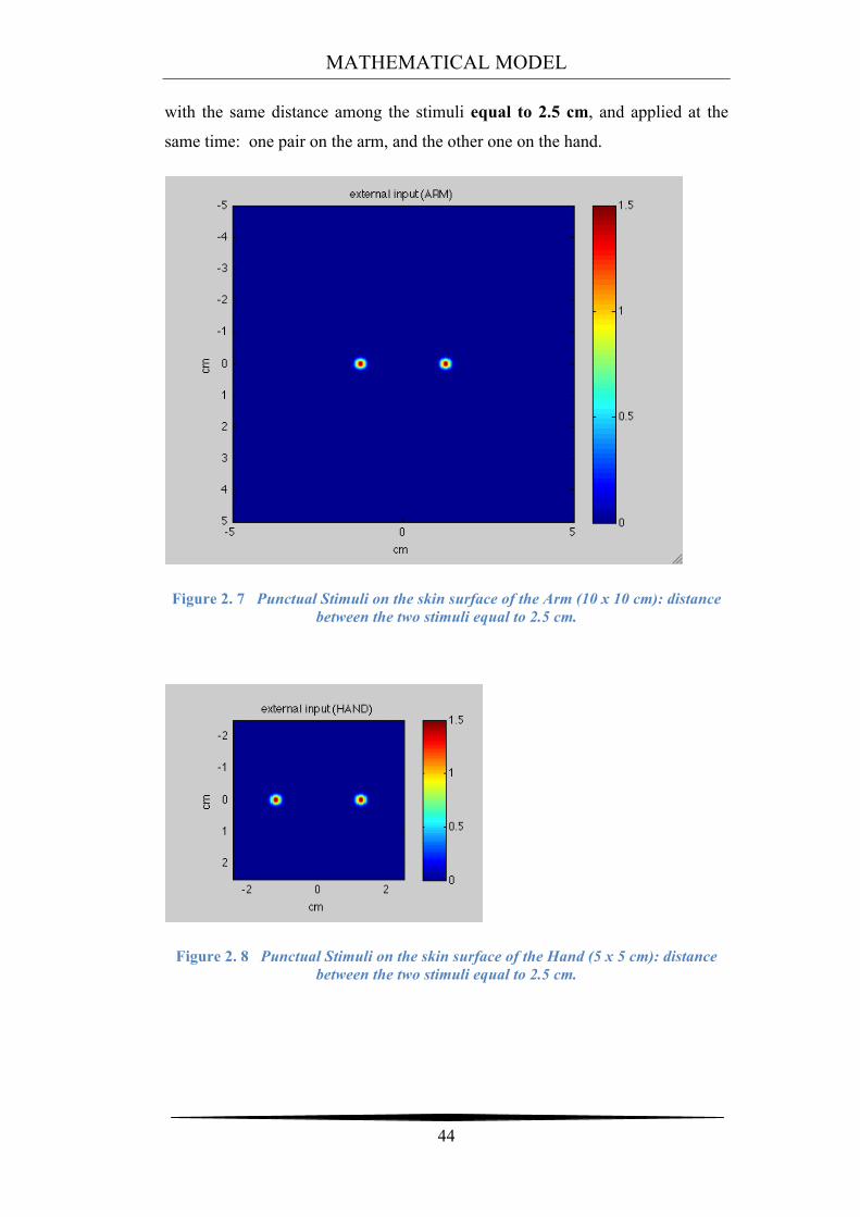
2.4 Activation of neurons step by step
The two stimuli were applied on a skin surface area of 5x5cm on the hand, and
10 x10 cm on the arm. In the s below it is possible to see two punctual stimuli,
MATHEMATICAL MODEL
44
with the same distance among the stimuli equal to 2.5 cm, and applied at the
same time: one pair on the arm, and the other one on the hand.
Figure 2. 7 Punctual Stimuli on the skin surface of the Arm (10 x 10 cm): distance between the two stimuli equal to 2.5 cm.
Figure 2. 8 Punctual Stimuli on the skin surface of the Hand (5 x 5 cm): distance between the two stimuli equal to 2.5 cm.
MATHEMATICAL MODEL
45
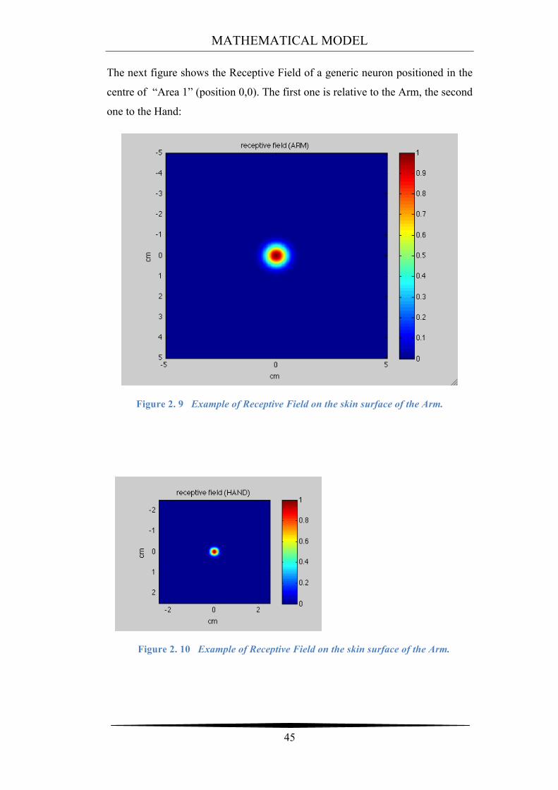
The next figure shows the Receptive Field of a generic neuron positioned in the
centre of “Area 1” (position 0,0). The first one is relative to the Arm, the second
one to the Hand:
Figure 2. 9 Example of Receptive Field on the skin surface of the Arm.
Figure 2. 10 Example of Receptive Field on the skin surface of the Arm.
MATHEMATICAL MODEL
46
It is evident the different size of the 2 Receptive Fields; the RF of a neuron
codifying stimuli on the Hand (Region A) covers a smaller skin surface than
neurons representing arm (Region B).
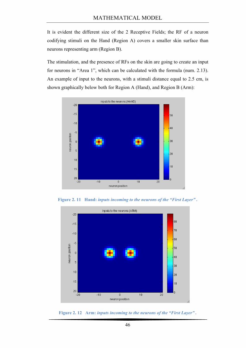
The stimulation, and the presence of RFs on the skin are going to create an input
for neurons in “Area 1”, which can be calculated with the formula (num. 2.13).
An example of input to the neurons, with a stimuli distance equal to 2.5 cm, is
shown graphically below both for Region A (Hand), and Region B (Arm):
Figure 2. 11 Hand: inputs incoming to the neurons of the “First Layer” .
Figure 2. 12 Arm: inputs incoming to the neurons of the “First Layer” .
MATHEMATICAL MODEL
47
Remember that these graphics do not represent the state of activation of the
neurons inside “Area 1”, but they just represent the effective neurons input. Each
little square is a neuron in “Area 1” and the colour is its input value. The colour
is associated with a value that can be consulted on the color bar. We can notice
that with the same distance of the input stimuli (2.5 cm), in the Arm’s case, the
bubbles are closer to each other, than the Hand’s case. Given that we have
simulated two different body regions, with different resolution, these results are
coherent with the reality. Remember that region A is an Area of 5 x 5 cm on the
Hand, whereas Region B is an Area equal to 10 x 10 cm on the Arm. In addition,
the cortical Areas linked with these two regions have the same dimension of 41
x 41 neurons; so, it is clear that Hand and Arm, have been interpreted by the
model as two regions with different resolution. In particular, the spatial
resolution of neurons for the two regions is:
• Hand 5 cm /41 neurons =
• Arm: 10 cm /41 neurons=
In Region A, the centers of neuron RFs are arranged at a distance of 0.12 cm,
whereas, in Region B, the centers of neuron RFs are arranged at a distance of
0.24 cm. Therefore, it is clear that the same distance of the input is represented
with different length, in terms of neurons, inside the cortical Areas.
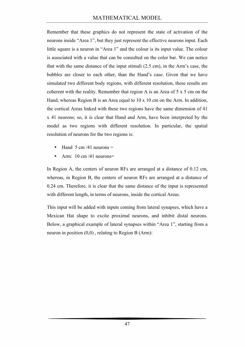
This input will be added with inputs coming from lateral synapses, which have a
Mexican Hat shape to excite proximal neurons, and inhibit distal neurons.
Below, a graphical example of lateral synapses within “Area 1”, starting from a
neuron in position (0,0) , relating to Region B (Arm):
MATHEMATICAL MODEL
48
Figure 2. 13 Arm: 2D view of Lateral Synapses within “Area 1”, starting from neuron in position (0,0).
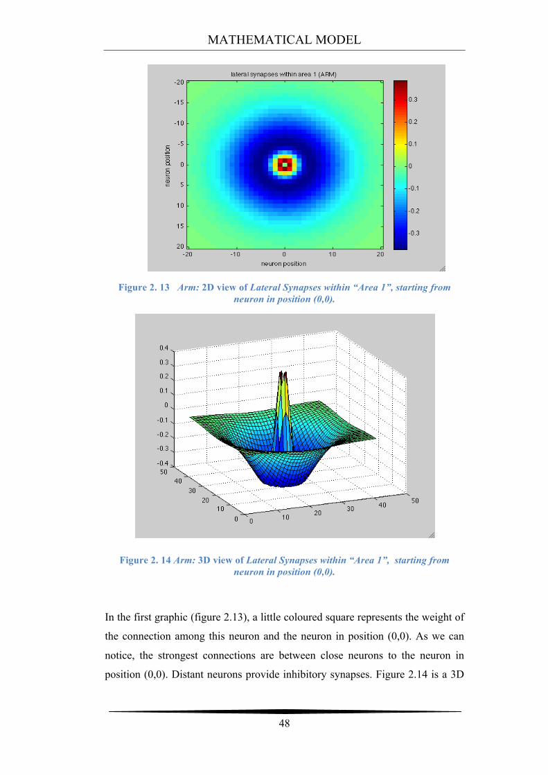
Figure 2. 14 Arm: 3D view of Lateral Synapses within “Area 1”, starting from neuron in position (0,0).
In the first graphic (figure 2.13), a little coloured square represents the weight of
the connection among this neuron and the neuron in position (0,0). As we can
notice, the strongest connections are between close neurons to the neuron in
position (0,0). Distant neurons provide inhibitory synapses. Figure 2.14 is a 3D
MATHEMATICAL MODEL
49
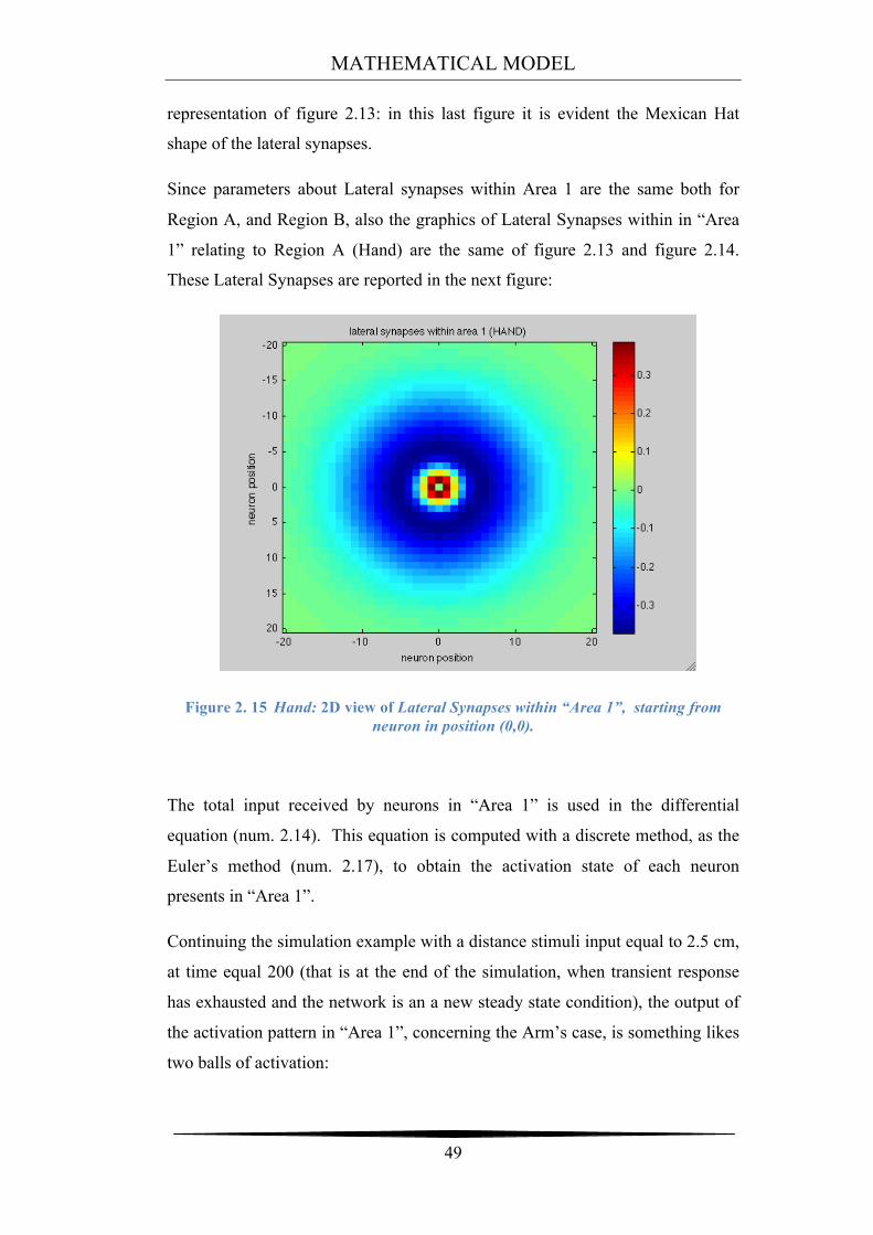
representation of figure 2.13: in this last figure it is evident the Mexican Hat
shape of the lateral synapses.
Since parameters about Lateral synapses within Area 1 are the same both for
Region A, and Region B, also the graphics of Lateral Synapses within in “Area
1” relating to Region A (Hand) are the same of figure 2.13 and figure 2.14.
These Lateral Synapses are reported in the next figure:
Figure 2. 15 Hand: 2D view of Lateral Synapses within “Area 1”, starting from neuron in position (0,0).
The total input received by neurons in “Area 1” is used in the differential
equation (num. 2.14). This equation is computed with a discrete method, as the
Euler’s method (num. 2.17), to obtain the activation state of each neuron
presents in “Area 1”.
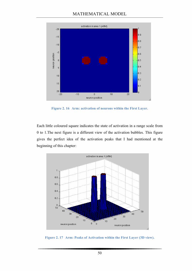
Continuing the simulation example with a distance stimuli input equal to 2.5 cm,
at time equal 200 (that is at the end of the simulation, when transient response
has exhausted and the network is an a new steady state condition), the output of
the activation pattern in “Area 1”, concerning the Arm’s case, is something likes
two balls of activation:
MATHEMATICAL MODEL
50
Figure 2. 16 Arm: activation of neurons within the First Layer.
Each little coloured square indicates the state of activation in a range scale from
0 to 1.The next figure is a different view of the activation bubbles. This figure
gives the perfect idea of the activation peaks that I had mentioned at the
beginning of this chapter:
Figure 2. 17 Arm: Peaks of Activation within the First Layer (3D view).
MATHEMATICAL MODEL
51
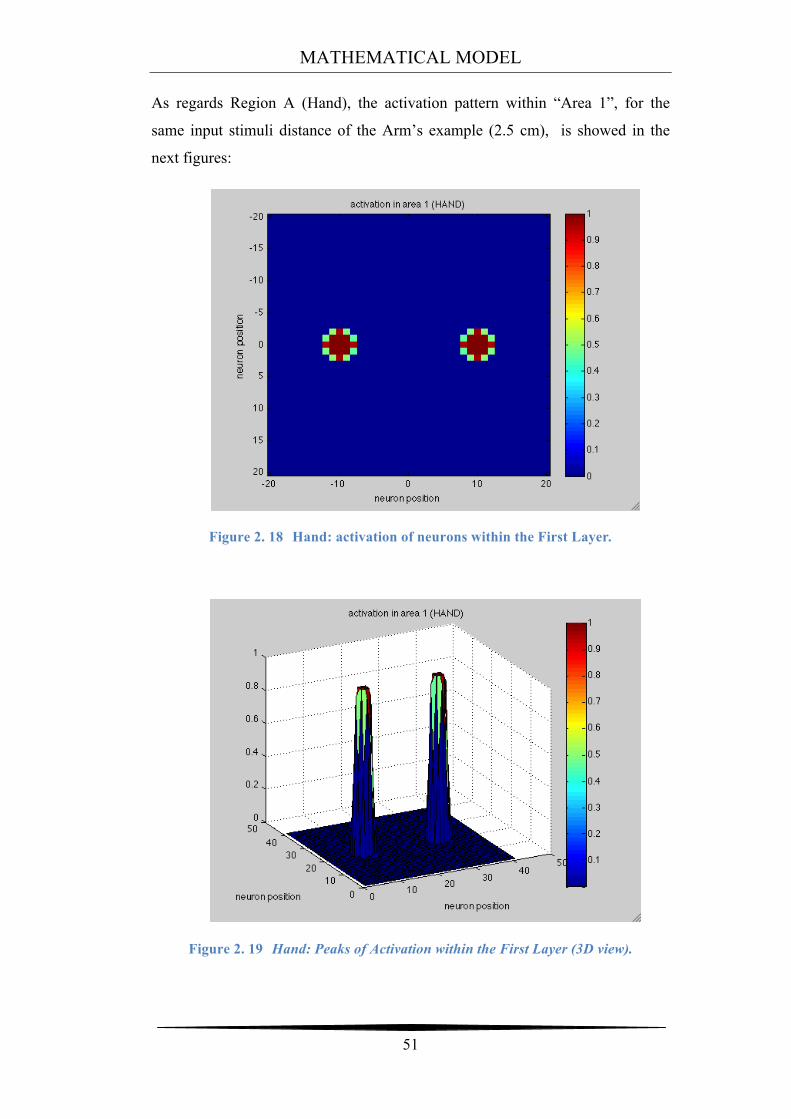
As regards Region A (Hand), the activation pattern within “Area 1”, for the
same input stimuli distance of the Arm’s example (2.5 cm), is showed in the
next figures:
Figure 2. 18 Hand: activation of neurons within the First Layer.
Figure 2. 19 Hand: Peaks of Activation within the First Layer (3D view).
MATHEMATICAL MODEL
52
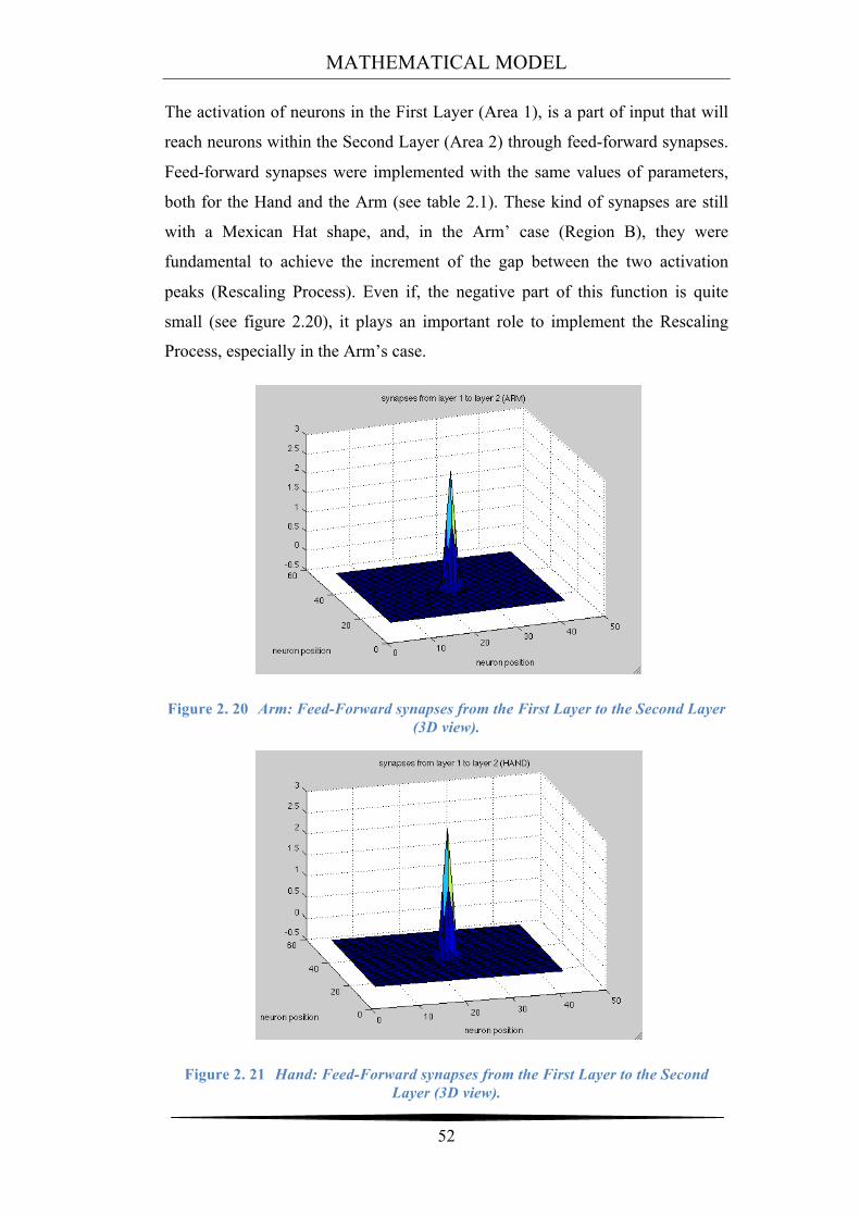
The activation of neurons in the First Layer (Area 1), is a part of input that will
reach neurons within the Second Layer (Area 2) through feed-forward synapses.
Feed-forward synapses were implemented with the same values of parameters,
both for the Hand and the Arm (see table 2.1). These kind of synapses are still
with a Mexican Hat shape, and, in the Arm’ case (Region B), they were
fundamental to achieve the increment of the gap between the two activation
peaks (Rescaling Process). Even if, the negative part of this function is quite
small (see figure 2.20), it plays an important role to implement the Rescaling
Process, especially in the Arm’s case.
Figure 2. 20 Arm: Feed-Forward synapses from the First Layer to the Second Layer (3D view).
Figure 2. 21 Hand: Feed-Forward synapses from the First Layer to the Second Layer (3D view).
MATHEMATICAL MODEL
53
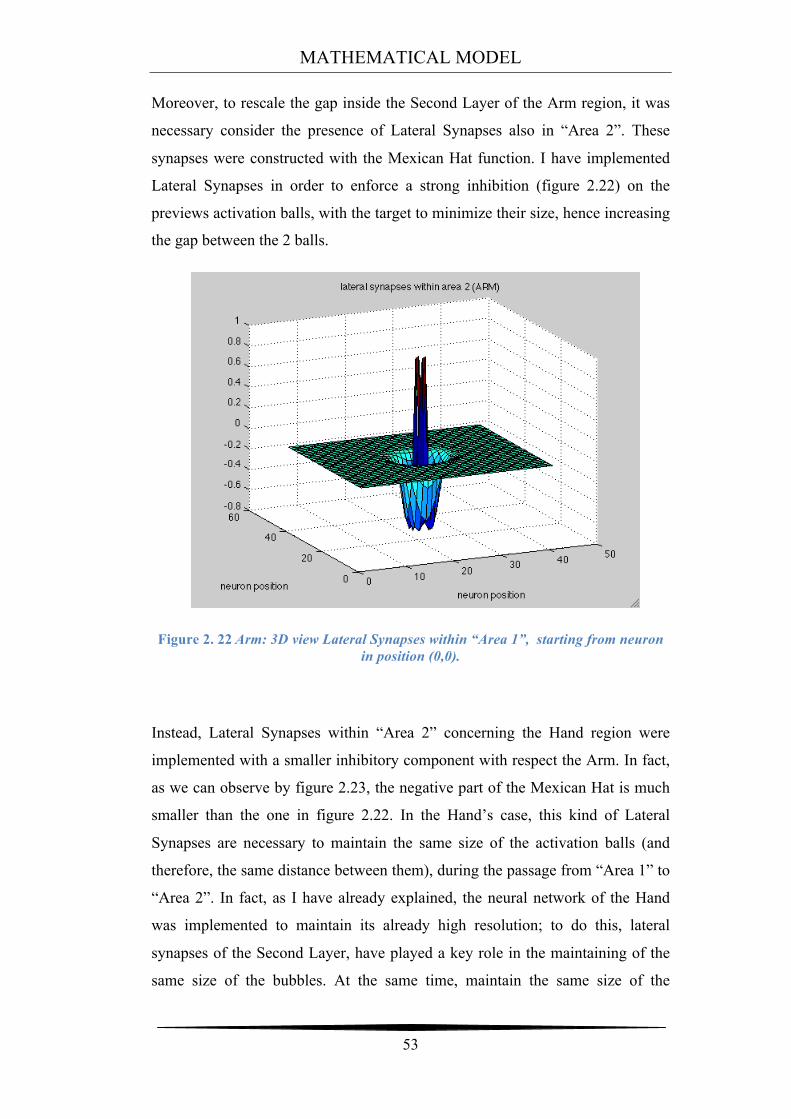
Moreover, to rescale the gap inside the Second Layer of the Arm region, it was
necessary consider the presence of Lateral Synapses also in “Area 2”. These
synapses were constructed with the Mexican Hat function. I have implemented
Lateral Synapses in order to enforce a strong inhibition (figure 2.22) on the
previews activation balls, with the target to minimize their size, hence increasing
the gap between the 2 balls.
Figure 2. 22 Arm: 3D view Lateral Synapses within “Area 1”, starting from neuron in position (0,0).
Instead, Lateral Synapses within “Area 2” concerning the Hand region were
implemented with a smaller inhibitory component with respect the Arm. In fact,
as we can observe by figure 2.23, the negative part of the Mexican Hat is much
smaller than the one in figure 2.22. In the Hand’s case, this kind of Lateral
Synapses are necessary to maintain the same size of the activation balls (and
therefore, the same distance between them), during the passage from “Area 1” to
“Area 2”. In fact, as I have already explained, the neural network of the Hand
was implemented to maintain its already high resolution; to do this, lateral
synapses of the Second Layer, have played a key role in the maintaining of the
same size of the bubbles. At the same time, maintain the same size of the
MATHEMATICAL MODEL
54
bubbles means keep constant the distance between the activation balls, that was
the target of the Hand’s neural network.
Figure 2. 23 Hand: 3D view Lateral Synapses within “Area 1”, starting from neuron in position (0,0).
Figure 2. 24 Different point of view of figure 2.22.
MATHEMATICAL MODEL
55
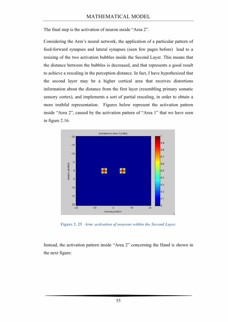
The final step is the activation of neuron inside “Area 2”.
Considering the Arm’s neural network, the application of a particular pattern of
feed-forward synapses and lateral synapses (seen few pages before) lead to a
resizing of the two activation bubbles inside the Second Layer. This means that
the distance between the bubbles is decreased, and that represents a good result
to achieve a rescaling in the perception distance. In fact, I have hypothesized that
the second layer may be a higher cortical area that receives distortions
information about the distance from the first layer (resembling primary somatic
sensory cortex), and implements a sort of partial rescaling, in order to obtain a
more truthful representation. Figures below represent the activation pattern
inside “Area 2”, caused by the activation pattern of “Area 1” that we have seen
in figure 2.16.
Figure 2. 25 Arm: activation of neurons within the Second Layer.
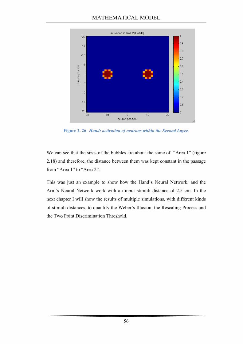
Instead, the activation pattern inside “Area 2” concerning the Hand is shown in
the next figure:
MATHEMATICAL MODEL
56
Figure 2. 26 Hand: activation of neurons within the Second Layer.
We can see that the sizes of the bubbles are about the same of “Area 1” (figure
2.18) and therefore, the distance between them was kept constant in the passage
from “Area 1” to “Area 2”.
This was just an example to show how the Hand’s Neural Network, and the
Arm’s Neural Network work with an input stimuli distance of 2.5 cm. In the
next chapter I will show the results of multiple simulations, with different kinds
of stimuli distances, to quantify the Weber’s Illusion, the Rescaling Process and
the Two Point Discrimination Threshold.
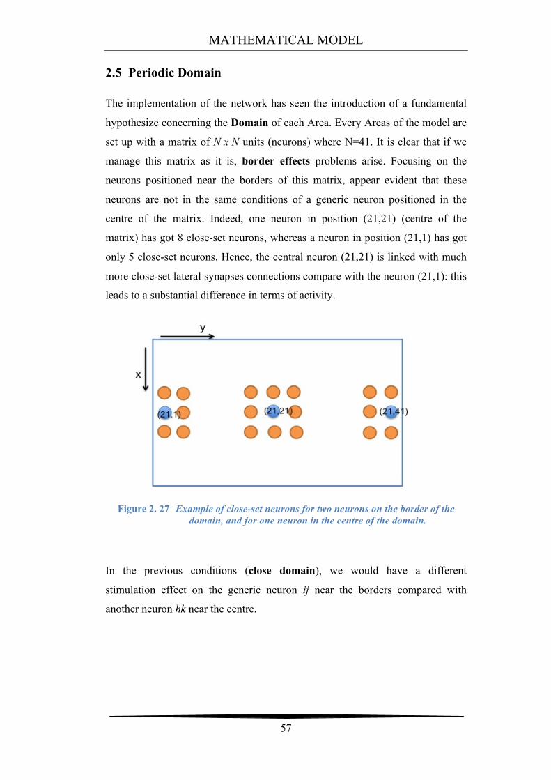
MATHEMATICAL MODEL
57
2.5 Periodic Domain
The implementation of the network has seen the introduction of a fundamental
hypothesize concerning the Domain of each Area. Every Areas of the model are
set up with a matrix of N x N units (neurons) where N=41. It is clear that if we
manage this matrix as it is, border effects problems arise. Focusing on the
neurons positioned near the borders of this matrix, appear evident that these
neurons are not in the same conditions of a generic neuron positioned in the
centre of the matrix. Indeed, one neuron in position (21,21) (centre of the
matrix) has got 8 close-set neurons, whereas a neuron in position (21,1) has got
only 5 close-set neurons. Hence, the central neuron (21,21) is linked with much
more close-set lateral synapses connections compare with the neuron (21,1): this
leads to a substantial difference in terms of activity.
Figure 2. 27 Example of close-set neurons for two neurons on the border of the domain, and for one neuron in the centre of the domain.
In the previous conditions (close domain), we would have a different
stimulation effect on the generic neuron ij near the borders compared with
another neuron hk near the centre.
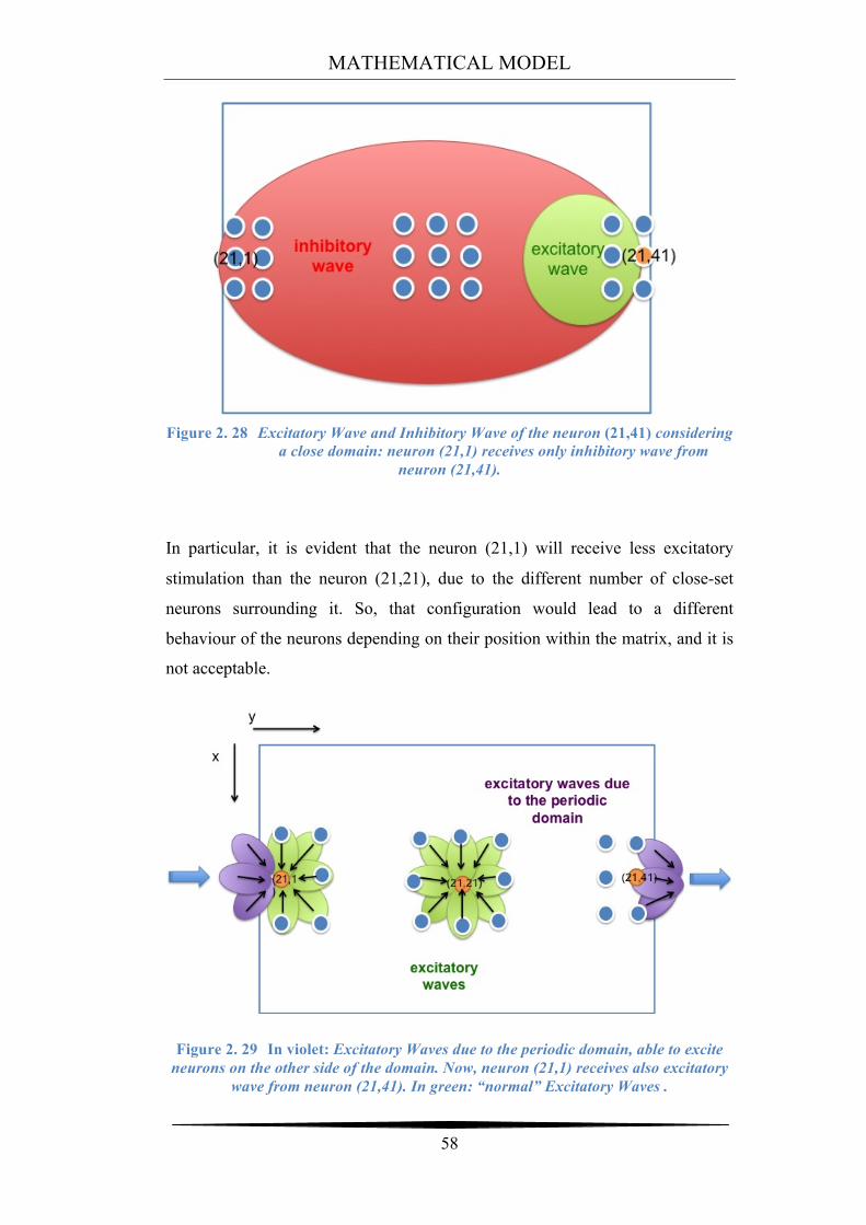
MATHEMATICAL MODEL
58
Figure 2. 28 Excitatory Wave and Inhibitory Wave of the neuron (21,41) considering a close domain: neuron (21,1) receives only inhibitory wave from
neuron (21,41).
In particular, it is evident that the neuron (21,1) will receive less excitatory
stimulation than the neuron (21,21), due to the different number of close-set
neurons surrounding it. So, that configuration would lead to a different
behaviour of the neurons depending on their position within the matrix, and it is
not acceptable.
Figure 2. 29 In violet: Excitatory Waves due to the periodic domain, able to excite neurons on the other side of the domain. Now, neuron (21,1) receives also excitatory
wave from neuron (21,41). In green: “normal” Excitatory Waves .
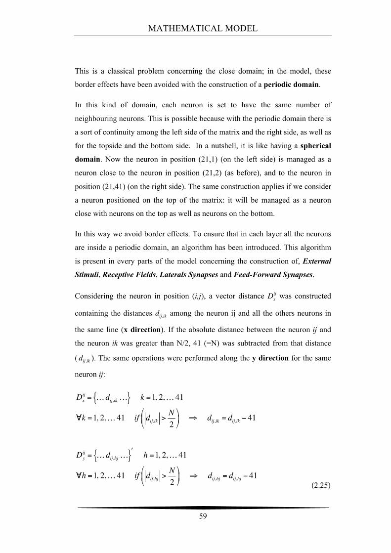
MATHEMATICAL MODEL
59
This is a classical problem concerning the close domain; in the model, these
border effects have been avoided with the construction of a periodic domain.
In this kind of domain, each neuron is set to have the same number of
neighbouring neurons. This is possible because with the periodic domain there is
a sort of continuity among the left side of the matrix and the right side, as well as
for the topside and the bottom side. In a nutshell, it is like having a spherical
domain. Now the neuron in position (21,1) (on the left side) is managed as a
neuron close to the neuron in position (21,2) (as before), and to the neuron in
position (21,41) (on the right side). The same construction applies if we consider
a neuron positioned on the top of the matrix: it will be managed as a neuron
close with neurons on the top as well as neurons on the bottom.
In this way we avoid border effects. To ensure that in each layer all the neurons
are inside a periodic domain, an algorithm has been introduced. This algorithm
is present in every parts of the model concerning the construction of, External
Stimuli, Receptive Fields, Laterals Synapses and Feed-Forward Synapses.
Considering the neuron in position (i,j), a vector distance Dxij was constructed
containing the distances dij,ik among the neuron ij and all the others neurons in
the same line (x direction). If the absolute distance between the neuron ij and
the neuron ik was greater than N/2, 41 (=N) was subtracted from that distance
( dij,ik ). The same operations were performed along the y direction for the same
neuron ij:
Dxij = … dij,ik…{ } k =1, 2,… 41
!k =1, 2,… 41 if dij,ik >N2
"
#$
%
&' ( dij,ik = dij,ik ) 41
Dijy = … dij,hj…{ }* h =1, 2,… 41
!h =1, 2,… 41 if dij,hj >N2
"
#$
%
&' ( dij,hj = dij,hj ) 41
(2.25)
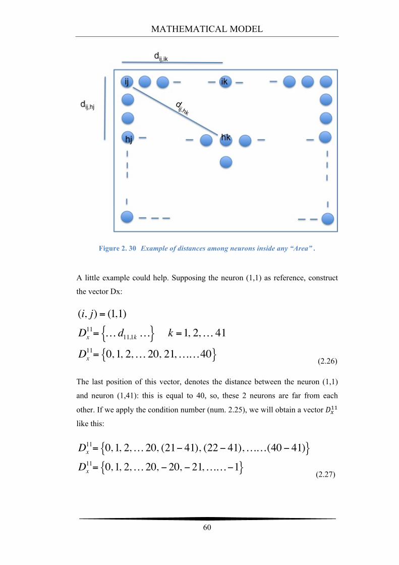
MATHEMATICAL MODEL
60
Figure 2. 30 Example of distances among neurons inside any “Area” .
A little example could help. Supposing the neuron (1,1) as reference, construct
the vector Dx:
(i, j) = (1,1)
Dx11= … d11,1k…{ } k =1, 2,… 41
Dx11= 0, 1, 2,…20, 21,……40{ } (2.26)
The last position of this vector, denotes the distance between the neuron (1,1)
and neuron (1,41): this is equal to 40, so, these 2 neurons are far from each
other. If we apply the condition number (num. 2.25), we will obtain a vector !!!!
like this:
Dx11= 0, 1, 2,…20, (21! 41), (22! 41),……(40! 41){ }
Dx11= 0, 1, 2,…20, ! 20, ! 21,……!1{ }
(2.27)
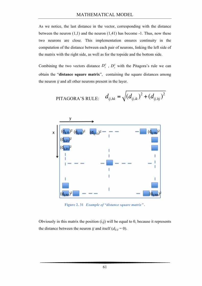
MATHEMATICAL MODEL
61
As we notice, the last distance in the vector, corresponding with the distance
between the neuron (1,1) and the neuron (1,41) has become -1. Thus, now these
two neurons are close. This implementation ensures continuity in the
computation of the distance between each pair of neurons, linking the left side of
the matrix with the right side, as well as for the topside and the bottom side.
Combining the two vectors distance , with the Pitagora’s rule we can
obtain the “distance square matrix”, containing the square distances among
the neuron ij and all other neurons present in the layer.
PITAGORA’S RULE: dij,hk = (dij,ik )2 + (dij,hj )
2
Figure 2. 31 Example of “distance square matrix” .
Obviously in this matrix the position (i,j) will be equal to 0, because it represents
the distance between the neuron ij and itself (dij,ij = 0).
Dxij Dij
y
62
Chapter 3
SIMULATIONS AND RESULTS
Introduction
In this chapter, all results of the simulations will be shown and they will be
analysed making tables, graphics and comparisons among them. Before starting
with the simulation results, a short panoramic view about the developed
environment of these simulations will be shown.
The neural network was implemented in MATLAB 7.9.0 environment. Different
programs in order to simulate the mechanisms of the perception of the distances
on Region A (hand), and Region B (Arm) have been implemented. Below, a
quick file list names with the relatives features:
• RegionA.m : allows to create a simulation concerning the mechanism of
perception of the distance between two punctual stimuli applied on the
hand. In this model, the skin region area is equal to 5 x 5 cm =25 cm2.
This is a deterministic neural network, because it does not simulate the
presence of noise in the parameters.
• RegionB.m : allows to create a simulation concerning the mechanism of
perception of the distance between 2 punctual stimuli applied on the arm.
The skin region simulated is equal to 10 x 10 cm =100 cm2. This is a
deterministic model because it does not simulate the presence of noise
in the parameters.
• Simulation.m: includes in a unique file RegionA.m and RegionB.m
programs, but it adds noise in some parameters, changing the network in
a stochastic model. This program repeats automatically the simulations
on both regions for 100 times, and for different distances between the
two stimuli, in order to record results in terms of perception distance and
make comparison among the two regions (hand and arm).
SIMULATIONS AND RESULTS
63
• ThresholdofPerceptionHand.m: is a program that computes the two
points discrimination threshold about the hand.
• ThresholdofPerceptionArm.m: is a program that computes the two points
discrimination threshold about the arm.
• CompareHandArm.m: loads data from ThresholdofPerceptionHand.m,
ThresholdofPerceptionArm.m and constructs graphics confronting the
different relations between distances in centimetres, and distances in
terms of number of neurons between the activation balls.
These were the main files used to perform simulations and to produce results.
Other important concepts, that have to be mentioned before starting with the
explanation of the neural network outputs, are linked with the noise that afflicts
some parameters, and the neuron activation threshold adopted to read out
perceived distance from the network activation.
The Noise
Focusing on the hand region, the activations inside the two layers could be
different in base on the distance between the two stimuli, and the intensity of the
two stimuli on the skin. So, if we change this kind of parameters we will obtain
different activation patterns within these layers. This is a very significant aspect
and it has to be managed. Just as in the reality, the application of two stimuli on
the skin of a subject, in two different trials, won’t be the same. That is because in
the reality it is almost impossible to replicate exactly the same experimental
conditions in different trials. For example the position of each stimulus could
change of few mm, as well as the intensity could change of few measure units.
Moreover, also neural activation is affected by noise.
To replicate these conditions, and reproduce external noise, and internal noise, it
was added noise in the parameters of the model. In particular, the noise was
superimposed to the position of each stimulus and to its amplitude (intensity of
the Gaussian function). The noise utilized in every simulation is a Gaussian
SIMULATIONS AND RESULTS
64
Noise, and it was generated by a MATLAB’s function called randn( ). For
example, using this formula:
! = ! + ! ∙ !"#$# 1,100 . (3.1)
we can create a vector x (in this case with a length equal to 100) of random
values, with a Normal Distribution that is defined by a mean value ! and
variance !!. With this equation, Gaussian noise in the position of the input and
in its amplitude (intensity) has been added. MATLAB’s instructions for the
construction of the position and the intensity of two stimuli are reported here:
inp1=inh1+0.3/2*randn(1,1); posizione_in_1=[inp1 0]; forza_in_1 =1.5+0.15*randn(1,1); inp2=inh2+0.3/2*randn(1,1); posizione_in_1=[inp1 0]; forza_in_2 =1.5+0.15*randn(1,1); inp1 and inp2 are the x coordinates for positions of the first stimulus and the
second stimulus respectively. Hence, if we want to simulate two stimuli at a
distance equal to 2.5 cm along the x axis, we have to impose:
• inp1 = -1.25 cm
• inp2 = 1.25 cm
since the position of the stimuli is referred to the center of the reference system.
This means that if we simulate a distance between the two stimuli of 2.5 cm for
100 times, the effective distance will not be always equal to 2.5 cm for every
trail, but sometimes it will be a bit greater and other times it will be a bit less
than 2.5 cm (it depends on the variance !! of the noise added to the position). In
particular, as indicated in the MATLAB instructions, the noise superimposed on
the stimulus position has 0 mean value, and 0.15 standard deviation Hence,
collecting all the 100 distances, we will notice that these distances are going to
spread as a Normal Distribution with mean ! and variance !!. However, also the
random intensity of the stimuli plays a key role in the patterns of activation
inside the first and the second layer. The noise superimposed on stimulus
intensity has 0 mean value and 0.15 standard deviation Therefore, the use of
SIMULATIONS AND RESULTS
65
noise helps in the reproduction of the real experiment condition, and changes the
model from a deterministic model to a stochastic model. “Stochastic" means
having a random variable. A stochastic model is a tool for estimating probability
distributions of potential outputs by allowing for random variation in one or
more inputs. Distributions of potential outputs are derived from a large number
of simulations (stochastic projections), which reflect the random variation in the
inputs.
Threshold of activation
In this chapter, when we will speak of distance between the two activation balls
in any layer, will consider the number of inactivated neurons between the two
activation balls (obviously the activation balls are composed by activated
neurons). The distinction among activated and inactivated neurons depends on a
threshold of activation. Given that the state variable (activation index of a
generic neuron) ranges from 0 to 1, in every simulation the threshold of
activation is always imposed equal 0.9. So, neurons with a value of the state
variable greater than 0.9 will be marked as activated neurons, otherwise as
inactivated neurons.
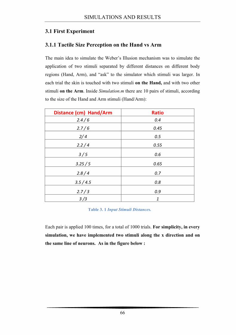
SIMULATIONS AND RESULTS
66
3.1 First Experiment
3.1.1 Tactile Size Perception on the Hand vs Arm
The main idea to simulate the Weber’s Illusion mechanism was to simulate the
application of two stimuli separated by different distances on different body
regions (Hand, Arm), and “ask” to the simulator which stimuli was larger. In
each trial the skin is touched with two stimuli on the Hand, and with two other
stimuli on the Arm. Inside Simulation.m there are 10 pairs of stimuli, according
to the size of the Hand and Arm stimuli (Hand/Arm):
Distance (cm) Hand/Arm Ratio 2.4 / 6 0.4
2.7 / 6 0.45
2/ 4 0.5
2.2 / 4 0.55
3 / 5 0.6
3.25 / 5 0.65
2.8 / 4 0.7
3.5 / 4.5 0.8
2.7 / 3 0.9 3 /3 1
Table 3. 1 Input Stimuli Distances.
Each pair is applied 100 times, for a total of 1000 trials. For simplicity, in every
simulation, we have implemented two stimuli along the x direction and on
the same line of neurons. As in the figure below :
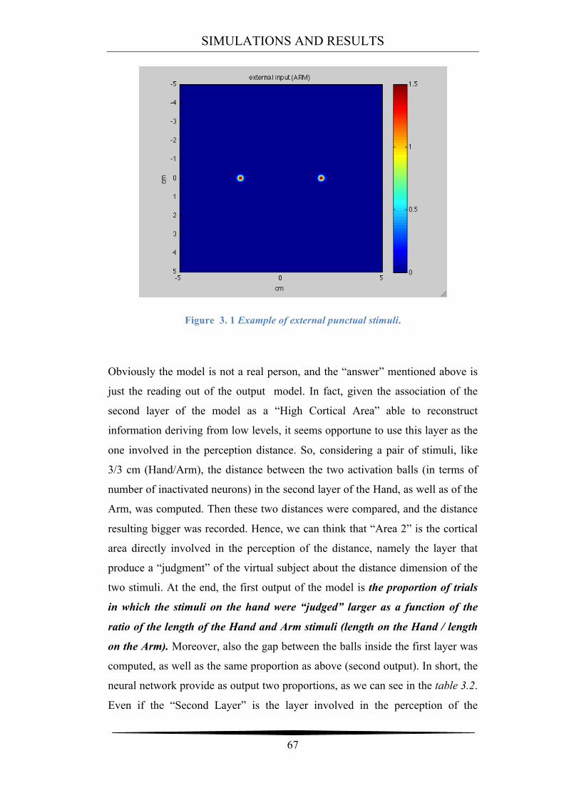
SIMULATIONS AND RESULTS
67
Figure 3. 1 Example of external punctual stimuli.
Obviously the model is not a real person, and the “answer” mentioned above is
just the reading out of the output model. In fact, given the association of the
second layer of the model as a “High Cortical Area” able to reconstruct
information deriving from low levels, it seems opportune to use this layer as the
one involved in the perception distance. So, considering a pair of stimuli, like
3/3 cm (Hand/Arm), the distance between the two activation balls (in terms of
number of inactivated neurons) in the second layer of the Hand, as well as of the
Arm, was computed. Then these two distances were compared, and the distance
resulting bigger was recorded. Hence, we can think that “Area 2” is the cortical
area directly involved in the perception of the distance, namely the layer that
produce a “judgment” of the virtual subject about the distance dimension of the
two stimuli. At the end, the first output of the model is the proportion of trials
in which the stimuli on the hand were “judged” larger as a function of the
ratio of the length of the Hand and Arm stimuli (length on the Hand / length
on the Arm). Moreover, also the gap between the balls inside the first layer was
computed, as well as the same proportion as above (second output). In short, the
neural network provide as output two proportions, as we can see in the table 3.2.
Even if the “Second Layer” is the layer involved in the perception of the
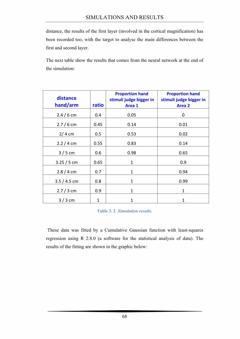
SIMULATIONS AND RESULTS
68
distance, the results of the first layer (involved in the cortical magnification) has
been recorded too, with the target to analyse the main differences between the
first and second layer.
The next table show the results that comes from the neural network at the end of
the simulation:
distance hand/arm ratio
Proportion hand stimuli judge bigger in
Area 1
Proportion hand stimuli judge bigger in
Area 2
2.4 / 6 cm 0.4 0.05 0
2.7 / 6 cm 0.45 0.14 0.01
2/ 4 cm 0.5 0.53 0.02
2.2 / 4 cm 0.55 0.83 0.14
3 / 5 cm 0.6 0.98 0.65
3.25 / 5 cm 0.65 1 0.9
2.8 / 4 cm 0.7 1 0.94
3.5 / 4.5 cm 0.8 1 0.99
2.7 / 3 cm 0.9 1 1
3 / 3 cm 1 1 1
Table 3. 2 Simulation results.
These data was fitted by a Cumulative Gaussian function with least-squares
regression using R 2.8.0 (a software for the statistical analysis of data). The
results of the fitting are shown in the graphic below:
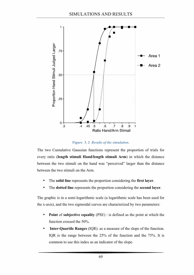
SIMULATIONS AND RESULTS
69
Figure 3. 2 Results of the simulation.
The two Cumulative Gaussian functions represent the proportion of trials for
every ratio (length stimuli Hand/length stimuli Arm) in which the distance
between the two stimuli on the hand was “perceived” larger than the distance
between the two stimuli on the Arm.
• The solid line represents the proportion considering the first layer.
• The dotted line represents the proportion considering the second layer.
The graphic is in a semi-logarithmic scale (a logarithmic scale has been used for
the x-axis), and the two sigmoidal curves are characterized by two parameters:
• Point of subjective equality (PSE) : is defined as the point at which the
function crossed the 50%.
• Inter-Quartile Ranges (IQR): as a measure of the slope of the function.
IQR is the range between the 25% of the function and the 75%. It is
common to use this index as an indicator of the slope.
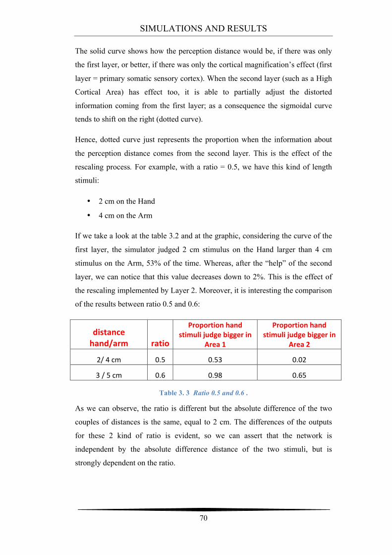
SIMULATIONS AND RESULTS
70
The solid curve shows how the perception distance would be, if there was only
the first layer, or better, if there was only the cortical magnification’s effect (first
layer = primary somatic sensory cortex). When the second layer (such as a High
Cortical Area) has effect too, it is able to partially adjust the distorted
information coming from the first layer; as a consequence the sigmoidal curve
tends to shift on the right (dotted curve).
Hence, dotted curve just represents the proportion when the information about
the perception distance comes from the second layer. This is the effect of the
rescaling process. For example, with a ratio = 0.5, we have this kind of length
stimuli:
• 2 cm on the Hand
• 4 cm on the Arm
If we take a look at the table 3.2 and at the graphic, considering the curve of the
first layer, the simulator judged 2 cm stimulus on the Hand larger than 4 cm
stimulus on the Arm, 53% of the time. Whereas, after the “help” of the second
layer, we can notice that this value decreases down to 2%. This is the effect of
the rescaling implemented by Layer 2. Moreover, it is interesting the comparison
of the results between ratio 0.5 and 0.6:
distance hand/arm ratio
Proportion hand stimuli judge bigger in
Area 1
Proportion hand stimuli judge bigger in
Area 2
2/ 4 cm 0.5 0.53 0.02
3 / 5 cm 0.6 0.98 0.65
Table 3. 3 Ratio 0.5 and 0.6 .
As we can observe, the ratio is different but the absolute difference of the two
couples of distances is the same, equal to 2 cm. The differences of the outputs
for these 2 kind of ratio is evident, so we can assert that the network is
independent by the absolute difference distance of the two stimuli, but is
strongly dependent on the ratio.
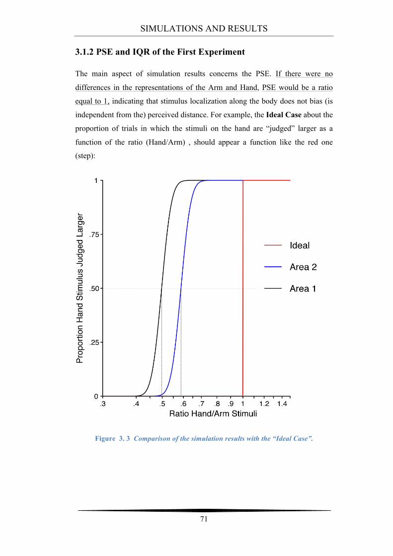
SIMULATIONS AND RESULTS
71
3.1.2 PSE and IQR of the First Experiment
The main aspect of simulation results concerns the PSE. If there were no
differences in the representations of the Arm and Hand, PSE would be a ratio
equal to 1, indicating that stimulus localization along the body does not bias (is
independent from the) perceived distance. For example, the Ideal Case about the
proportion of trials in which the stimuli on the hand are “judged” larger as a
function of the ratio (Hand/Arm) , should appear a function like the red one
(step):
Figure 3. 3 Comparison of the simulation results with the “Ideal Case”.
SIMULATIONS AND RESULTS
72
In the Ideal curve, PSE is equal to 1 and the slope of its curve is infinity. PSE is
equal 1 because, if we think to apply the same pair of distances, for example 3/3
cm (Hand/Arm) , 100 times on the skin surface of the subject, the subject will
judge larger the stimuli on the hand approximately half of the times, whereas in
the other half of the times he will judge larger the stimuli on the arm. This
because the two stimuli are equals, and the subject is not able to discriminate
between them (that is, he will answer at chance). Instead, the slope of the ideal
curve is infinity (like a step) simply because in an ideal condition, the subject is
able to classify correctly each couple of distances, with an extremely high
precision. Namely, in this condition the subject can understand correctly if the
stimulus on the hand is bigger than the stimulus on the arm. In fact, for every
ratio smaller than 1 (that means stimuli on the hand smaller than stimuli on the
arm), the curve is equal 0, whereas, for every ratio bigger than 1 the curve is
constant equal to 1. However, the Weber’s Illusion comes from a distortion of
the body shape, resulting in a sort of alteration in the judgment of which
stimulus is larger. This alteration tends to shift the curve toward smaller ratios
(black and blue curve), and the PSE of this curve is going to be smaller than the
ideal case. In addition, the slope of these curves won’t be equal to infinity,
because the subject tends to misperceive the real dimension of the stimuli.
So, we can assert that the Weber’s illusion is directly related with the shift
of the PSE toward smaller ratio, whereas the precision in the judgment of
which stimulus (on the hand or on the Arm) is bigger, is linked with the
slope of the sigmoidal curve. The shift of the PSE (or the curve in general) is
also called bias.
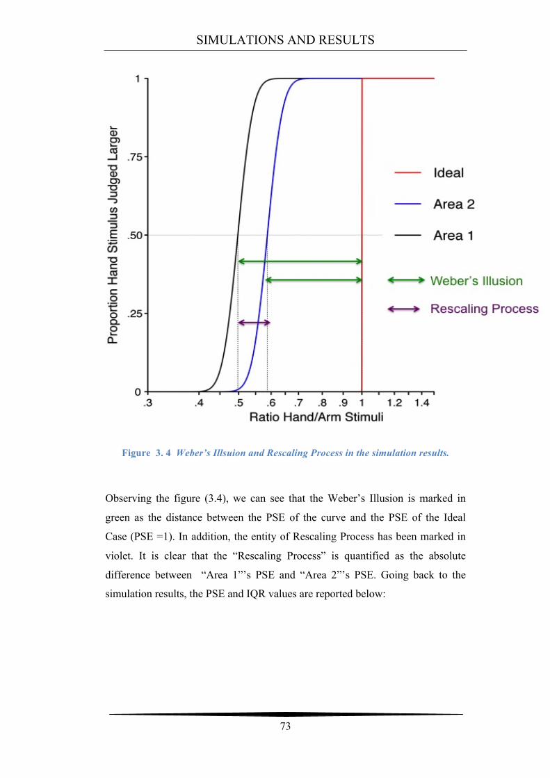
SIMULATIONS AND RESULTS
73
Figure 3. 4 Weber’s Illsuion and Rescaling Process in the simulation results.
Observing the figure (3.4), we can see that the Weber’s Illusion is marked in
green as the distance between the PSE of the curve and the PSE of the Ideal
Case (PSE =1). In addition, the entity of Rescaling Process has been marked in
violet. It is clear that the “Rescaling Process” is quantified as the absolute
difference between “Area 1”’s PSE and “Area 2”’s PSE. Going back to the
simulation results, the PSE and IQR values are reported below:
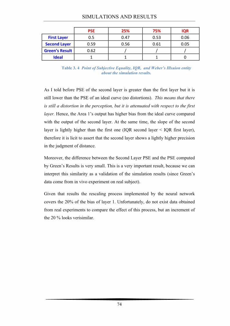
SIMULATIONS AND RESULTS
74
PSE 25% 75% IQR
First Layer 0.5 0.47 0.53 0.06 Second Layer 0.59 0.56 0.61 0.05 Green’s Result 0.62 / / /
Ideal 1 1 1 0
Table 3. 4 Point of Subjective Equality, IQR, and Weber’s Illsuion entity about the simulation results.
As I told before PSE of the second layer is greater than the first layer but it is
still lower than the PSE of an ideal curve (no distortions). This means that there
is still a distortion in the perception, but it is attenuated with respect to the first
layer. Hence, the Area 1’s output has higher bias from the ideal curve compared
with the output of the second layer. At the same time, the slope of the second
layer is lightly higher than the first one (IQR second layer < IQR first layer),
therefore it is licit to assert that the second layer shows a lightly higher precision
in the judgment of distance.
Moreover, the difference between the Second Layer PSE and the PSE computed
by Green’s Results is very small. This is a very important result, because we can
interpret this similarity as a validation of the simulation results (since Green’s
data come from in vivo experiment on real subject).
Given that results the rescaling process implemented by the neural network
covers the 20% of the bias of layer 1. Unfortunately, do not exist data obtained
from real experiments to compare the effect of this process, but an increment of
the 20 % looks verisimilar.
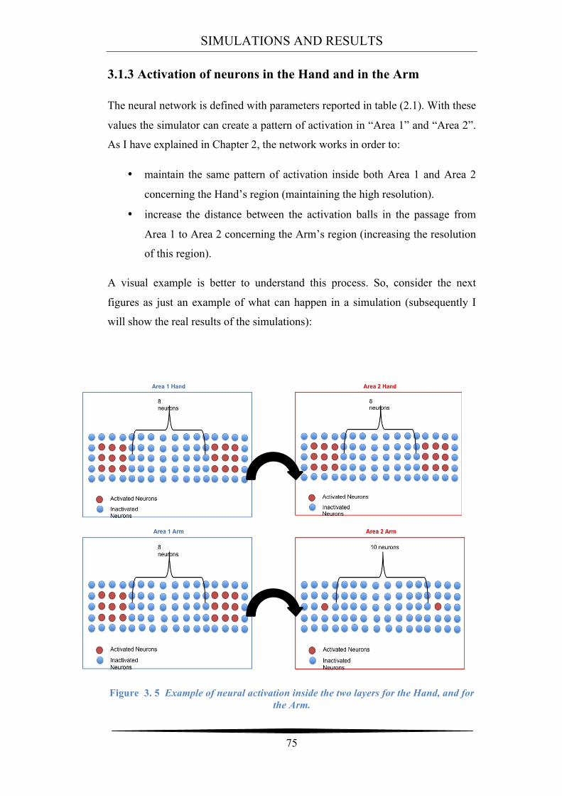
SIMULATIONS AND RESULTS
75
3.1.3 Activation of neurons in the Hand and in the Arm
The neural network is defined with parameters reported in table (2.1). With these
values the simulator can create a pattern of activation in “Area 1” and “Area 2”.
As I have explained in Chapter 2, the network works in order to:
• maintain the same pattern of activation inside both Area 1 and Area 2
concerning the Hand’s region (maintaining the high resolution).
• increase the distance between the activation balls in the passage from
Area 1 to Area 2 concerning the Arm’s region (increasing the resolution
of this region).
A visual example is better to understand this process. So, consider the next
figures as just an example of what can happen in a simulation (subsequently I
will show the real results of the simulations):
Figure 3. 5 Example of neural activation inside the two layers for the Hand, and for the Arm.
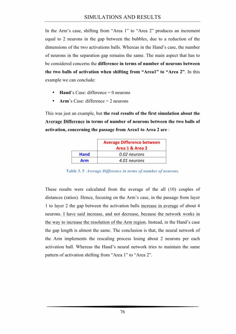
SIMULATIONS AND RESULTS
76
In the Arm’s case, shifting from “Area 1” to “Area 2” produces an increment
equal to 2 neurons in the gap between the bubbles, due to a reduction of the
dimensions of the two activations balls. Whereas in the Hand’s case, the number
of neurons in the separation gap remains the same. The main aspect that has to
be considered concerns the difference in terms of number of neurons between
the two balls of activation when shifting from “Area1” to “Area 2”. In this
example we can conclude:
• Hand’s Case: difference = 0 neurons
• Arm’s Case: difference = 2 neurons
This was just an example, but the real results of the first simulation about the
Average Difference in terms of number of neurons between the two balls of
activation, concerning the passage from Area1 to Area 2 are :
Average Difference between Area 1 & Area 2
Hand 0.02 neurons Arm 4.01 neurons
Table 3. 5 Average Difference in terms of number of neurons.
These results were calculated from the average of the all (10) couples of
distances (ratios). Hence, focusing on the Arm’s case, in the passage from layer
1 to layer 2 the gap between the activation balls increase in average of about 4
neurons. I have said increase, and not decrease, because the network works in
the way to increase the resolution of the Arm region. Instead, in the Hand’s case
the gap length is almost the same. The conclusion is that, the neural network of
the Arm implements the rescaling process losing about 2 neurons per each
activation ball. Whereas the Hand’s neural network tries to maintain the same
pattern of activation shifting from “Area 1” to “Area 2”.
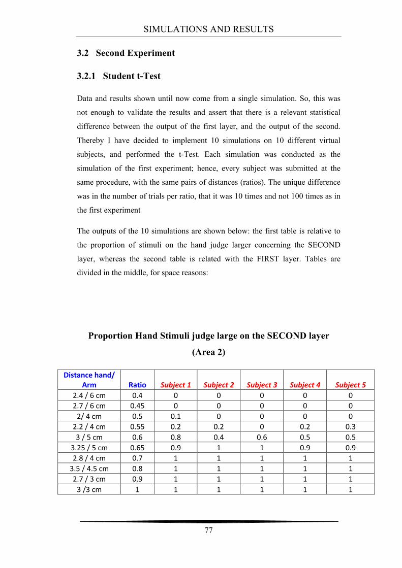
SIMULATIONS AND RESULTS
77
3.2 Second Experiment
3.2.1 Student t-Test
Data and results shown until now come from a single simulation. So, this was
not enough to validate the results and assert that there is a relevant statistical
difference between the output of the first layer, and the output of the second.
Thereby I have decided to implement 10 simulations on 10 different virtual
subjects, and performed the t-Test. Each simulation was conducted as the
simulation of the first experiment; hence, every subject was submitted at the
same procedure, with the same pairs of distances (ratios). The unique difference
was in the number of trials per ratio, that it was 10 times and not 100 times as in
the first experiment
The outputs of the 10 simulations are shown below: the first table is relative to
the proportion of stimuli on the hand judge larger concerning the SECOND
layer, whereas the second table is related with the FIRST layer. Tables are
divided in the middle, for space reasons:
Proportion Hand Stimuli judge large on the SECOND layer
(Area 2)
Distance hand/ Arm Ratio Subject 1 Subject 2 Subject 3 Subject 4 Subject 5
2.4 / 6 cm 0.4 0 0 0 0 0 2.7 / 6 cm 0.45 0 0 0 0 0 2/ 4 cm 0.5 0.1 0 0 0 0 2.2 / 4 cm 0.55 0.2 0.2 0 0.2 0.3 3 / 5 cm 0.6 0.8 0.4 0.6 0.5 0.5
3.25 / 5 cm 0.65 0.9 1 1 0.9 0.9 2.8 / 4 cm 0.7 1 1 1 1 1 3.5 / 4.5 cm 0.8 1 1 1 1 1 2.7 / 3 cm 0.9 1 1 1 1 1 3 /3 cm 1 1 1 1 1 1
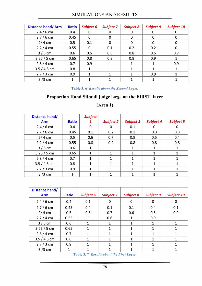
SIMULATIONS AND RESULTS
78
Distance hand/ Arm Ratio Subject 6 Subject 7 Subject 8 Subject 9 Subject 10 2.4 / 6 cm 0.4 0 0 0 0 0 2.7 / 6 cm 0.45 0 0 0 0 0 2/ 4 cm 0.5 0.1 0 0 0 0 2.2 / 4 cm 0.55 0 0.1 0.2 0.2 0 3 / 5 cm 0.6 0.5 0.6 0.8 0.5 0.7
3.25 / 5 cm 0.65 0.8 0.9 0.8 0.9 1 2.8 / 4 cm 0.7 0.9 1 1 1 0.9 3.5 / 4.5 cm 0.8 1 1 1 1 1 2.7 / 3 cm 0.9 1 1 1 0.9 1 3 /3 cm 1 1 1 1 1 1
Table 3. 6 Results about the Second Layer.
Proportion Hand Stimuli judge large on the FIRST layer
(Area 1)
Distance hand/ Arm Ratio
Subject 1 Subject 2 Subject 3 Subject 4 Subject 5
2.4 / 6 cm 0.4 0 0 0.1 0 0 2.7 / 6 cm 0.45 0.1 0.2 0.1 0.3 0.3 2/ 4 cm 0.5 0.6 0.7 0.8 0.5 0.4 2.2 / 4 cm 0.55 0.8 0.9 0.8 0.8 0.8 3 / 5 cm 0.6 1 1 1 1 1
3.25 / 5 cm 0.65 1 1 1 1 1 2.8 / 4 cm 0.7 1 1 1 1 1 3.5 / 4.5 cm 0.8 1 1 1 1 1 2.7 / 3 cm 0.9 1 1 1 1 1 3 /3 cm 1 1 1 1 1 1
Distance hand/ Arm Ratio Subject 6 Subject 7 Subject 8 Subject 9 Subject 10
2.4 / 6 cm 0.4 0.1 0 0 0 0 2.7 / 6 cm 0.45 0.4 0.1 0.1 0.4 0.1 2/ 4 cm 0.5 0.5 0.7 0.6 0.5 0.9 2.2 / 4 cm 0.55 1 0.6 1 0.9 1 3 / 5 cm 0.6 1 1 1 1 1
3.25 / 5 cm 0.65 1 1 1 1 1 2.8 / 4 cm 0.7 1 1 1 1 1 3.5 / 4.5 cm 0.8 1 1 1 1 1 2.7 / 3 cm 0.9 1 1 1 1 1 3 /3 cm 1 1 1 1 1 1
Table 3. 7 Results about the First Layer.
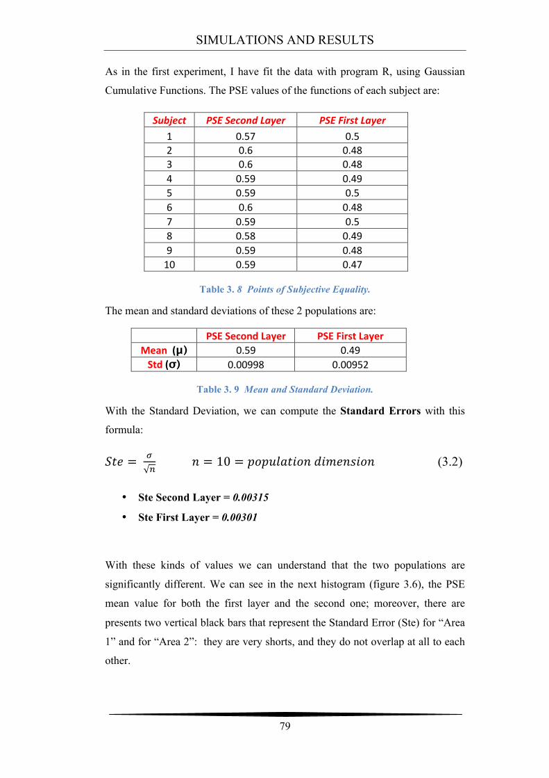
SIMULATIONS AND RESULTS
79
As in the first experiment, I have fit the data with program R, using Gaussian
Cumulative Functions. The PSE values of the functions of each subject are:
Subject PSE Second Layer PSE First Layer 1 0.57 0.5 2 0.6 0.48 3 0.6 0.48 4 0.59 0.49 5 0.59 0.5 6 0.6 0.48 7 0.59 0.5 8 0.58 0.49 9 0.59 0.48 10 0.59 0.47
Table 3. 8 Points of Subjective Equality.
The mean and standard deviations of these 2 populations are:
PSE Second Layer PSE First Layer
Mean (μ) 0.59 0.49 Std (σ) 0.00998 0.00952
Table 3. 9 Mean and Standard Deviation.
With the Standard Deviation, we can compute the Standard Errors with this
formula:
!"# = !! ! = 10 = !"!#$%&'"( !"#$%&"'% (3.2)
• Ste Second Layer = 0.00315
• Ste First Layer = 0.00301
With these kinds of values we can understand that the two populations are
significantly different. We can see in the next histogram (figure 3.6), the PSE
mean value for both the first layer and the second one; moreover, there are
presents two vertical black bars that represent the Standard Error (Ste) for “Area
1” and for “Area 2”: they are very shorts, and they do not overlap at all to each
other.
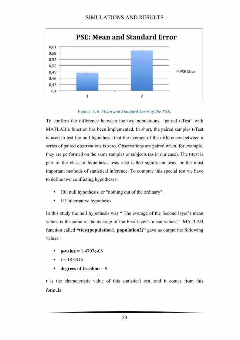
SIMULATIONS AND RESULTS
80
Figure 3. 6 Mean and Standard Error of the PSE.
To confirm the difference between the two populations, “paired t-Test” with
MATLAB’s function has been implemented. In short, the paired samples t-Test
is used to test the null hypothesis that the average of the differences between a
series of paired observations is zero. Observations are paired when, for example,
they are performed on the same samples or subjects (as in our case). The t-test is
part of the class of hypothesis tests also called significant tests, or the most
important methods of statistical inference. To compute this special test we have
to define two conflicting hypotheses:
• H0: null hypothesis, or "nothing out of the ordinary".
• H1: alternative hypothesis.
In this study the null hypothesis was “ The average of the Second layer’s mean
values is the same of the average of the First layer’s mean values”. MATLAB
function called “ttest(population1, population2)” gave as output the following
values:
• p-value = 1.4707e-08
• t = 18.9346
• degrees of freedom = 9
t is the characteristic value of this statistical test, and it comes from this
formula:
0,4 0,43 0,46 0,49 0,52 0,55 0,58 0,61
1 2
PSE: Mean and Standard Error
PSE Mean
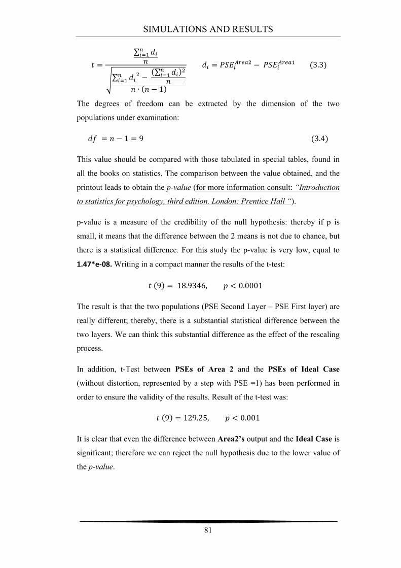
SIMULATIONS AND RESULTS
81
! =!!!
!!!!
!!! − !!!
!!!!
!!!!!
! ∙ ! − 1
!! = !"#!!"#$! − !"#!!"#$! (3.3)
The degrees of freedom can be extracted by the dimension of the two
populations under examination:
!" = ! − 1 = 9 (3.4)
This value should be compared with those tabulated in special tables, found in
all the books on statistics. The comparison between the value obtained, and the
printout leads to obtain the p-value (for more information consult: “Introduction
to statistics for psychology, third edition. London: Prentice Hall “).
p-value is a measure of the credibility of the null hypothesis: thereby if p is
small, it means that the difference between the 2 means is not due to chance, but
there is a statistical difference. For this study the p-value is very low, equal to
1.47*e-‐08. Writing in a compact manner the results of the t-test:
! 9 = 18.9346, ! < 0.0001
The result is that the two populations (PSE Second Layer – PSE First layer) are
really different; thereby, there is a substantial statistical difference between the
two layers. We can think this substantial difference as the effect of the rescaling
process.
In addition, t-Test between PSEs of Area 2 and the PSEs of Ideal Case
(without distortion, represented by a step with PSE =1) has been performed in
order to ensure the validity of the results. Result of the t-test was:
! 9 = 129.25, ! < 0.001
It is clear that even the difference between Area2’s output and the Ideal Case is
significant; therefore we can reject the null hypothesis due to the lower value of
the p-value.
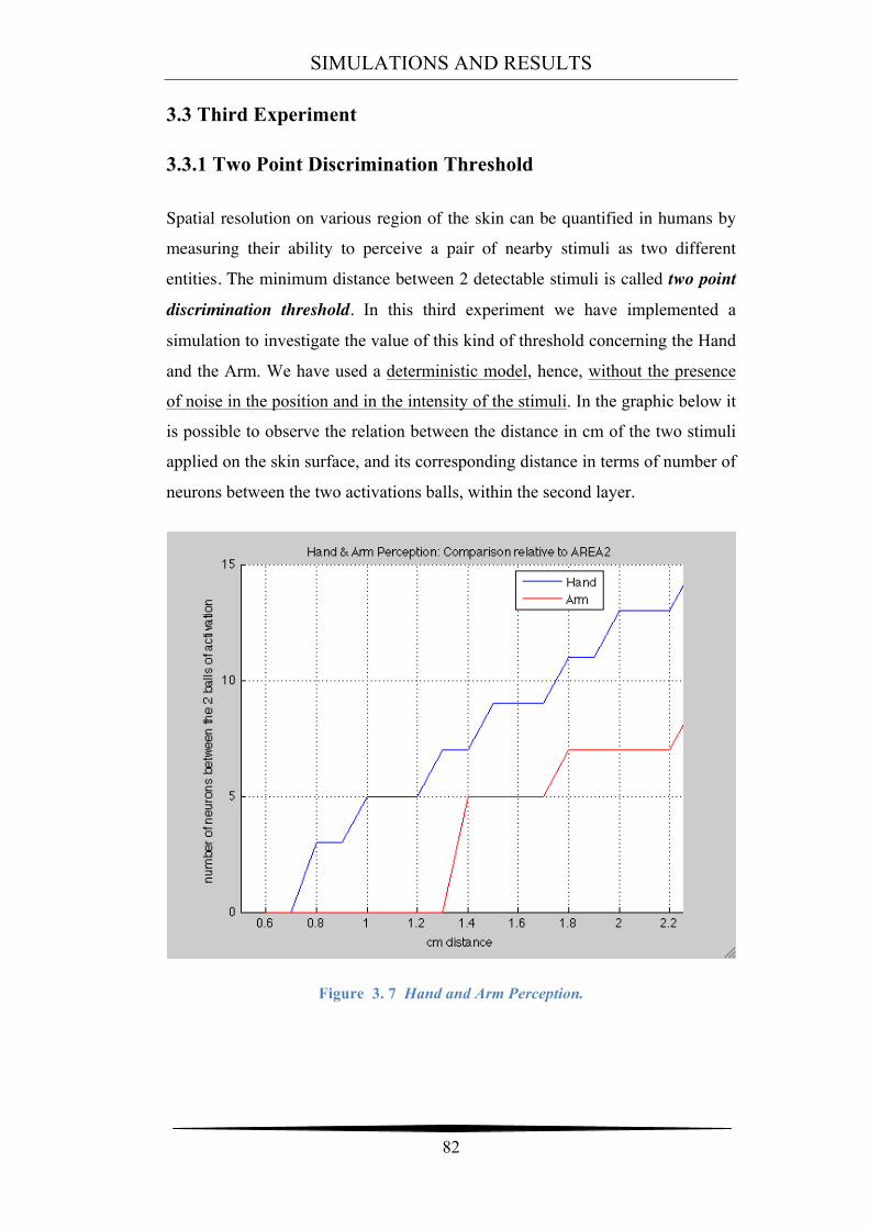
SIMULATIONS AND RESULTS
82
3.3 Third Experiment
3.3.1 Two Point Discrimination Threshold
Spatial resolution on various region of the skin can be quantified in humans by
measuring their ability to perceive a pair of nearby stimuli as two different
entities. The minimum distance between 2 detectable stimuli is called two point
discrimination threshold. In this third experiment we have implemented a
simulation to investigate the value of this kind of threshold concerning the Hand
and the Arm. We have used a deterministic model, hence, without the presence
of noise in the position and in the intensity of the stimuli. In the graphic below it
is possible to observe the relation between the distance in cm of the two stimuli
applied on the skin surface, and its corresponding distance in terms of number of
neurons between the two activations balls, within the second layer.
Figure 3. 7 Hand and Arm Perception.
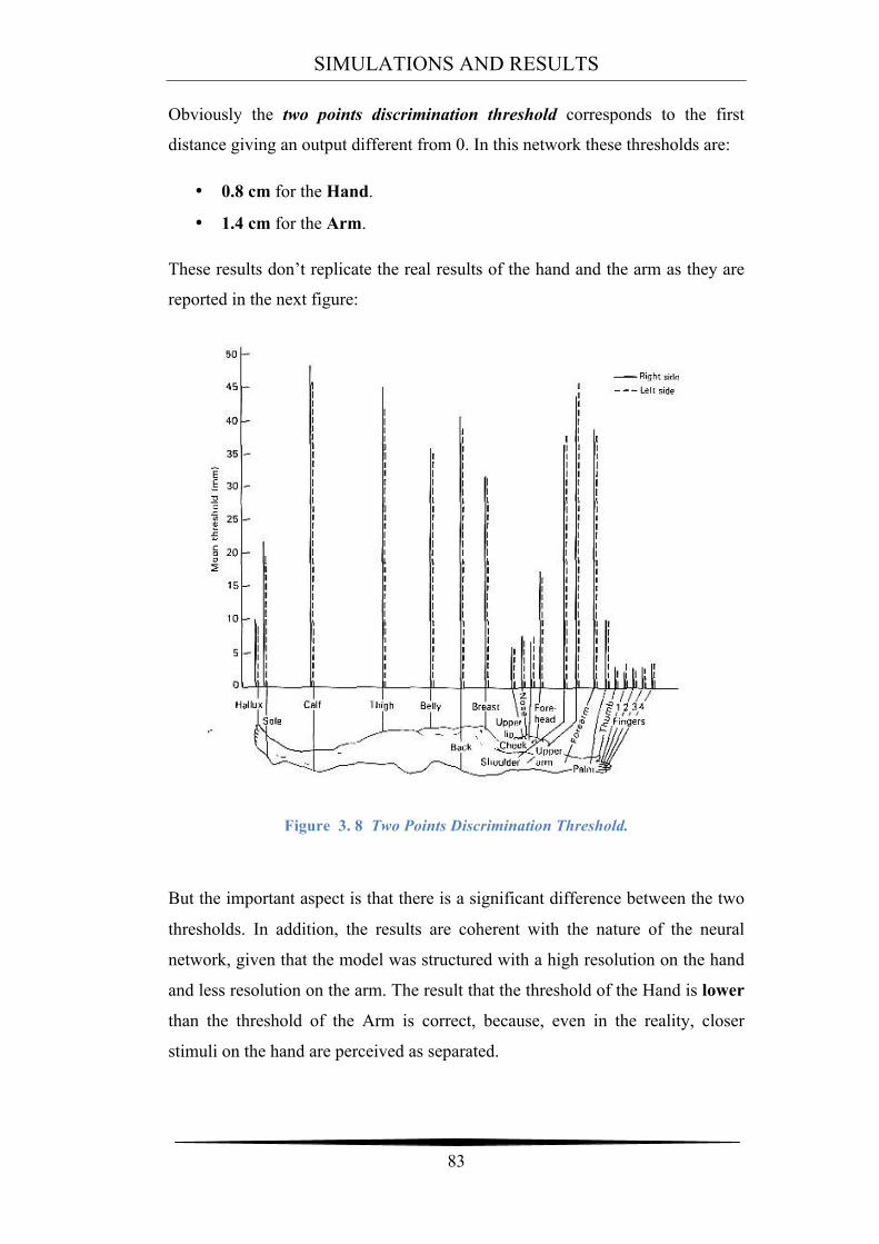
SIMULATIONS AND RESULTS
83
Obviously the two points discrimination threshold corresponds to the first
distance giving an output different from 0. In this network these thresholds are:
• 0.8 cm for the Hand.
• 1.4 cm for the Arm.
These results don’t replicate the real results of the hand and the arm as they are
reported in the next figure:
Figure 3. 8 Two Points Discrimination Threshold.
But the important aspect is that there is a significant difference between the two
thresholds. In addition, the results are coherent with the nature of the neural
network, given that the model was structured with a high resolution on the hand
and less resolution on the arm. The result that the threshold of the Hand is lower
than the threshold of the Arm is correct, because, even in the reality, closer
stimuli on the hand are perceived as separated.
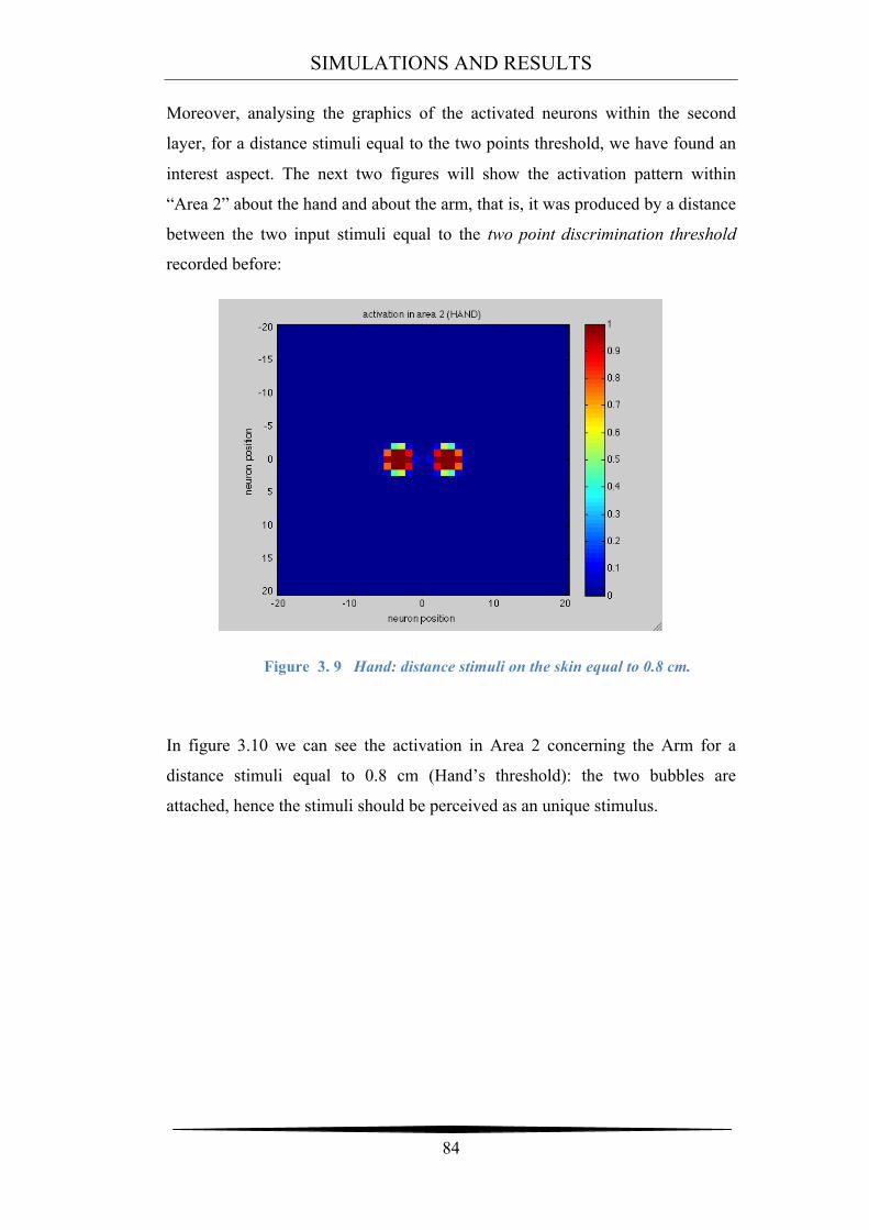
SIMULATIONS AND RESULTS
84
Moreover, analysing the graphics of the activated neurons within the second
layer, for a distance stimuli equal to the two points threshold, we have found an
interest aspect. The next two figures will show the activation pattern within
“Area 2” about the hand and about the arm, that is, it was produced by a distance
between the two input stimuli equal to the two point discrimination threshold
recorded before:
Figure 3. 9 Hand: distance stimuli on the skin equal to 0.8 cm.
In figure 3.10 we can see the activation in Area 2 concerning the Arm for a
distance stimuli equal to 0.8 cm (Hand’s threshold): the two bubbles are
attached, hence the stimuli should be perceived as an unique stimulus.
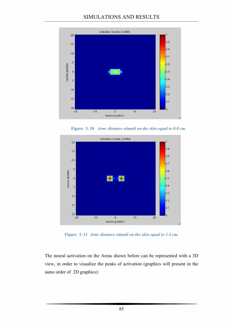
SIMULATIONS AND RESULTS
85
Figure 3. 10 Arm: distance stimuli on the skin equal to 0.8 cm.
Figure 3. 11 Arm: distance stimuli on the skin equal to 1.4 cm.
The neural activation on the Areas shown before can be represented with a 3D
view, in order to visualize the peaks of activation (graphics will present in the
same order of 2D graphics):
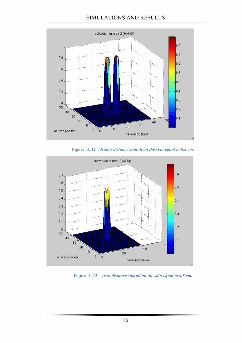
SIMULATIONS AND RESULTS
86
Figure 3. 12 Hand: distance stimuli on the skin equal to 0.8 cm.
Figure 3. 13 Arm: distance stimuli on the skin equal to 0.8 cm.
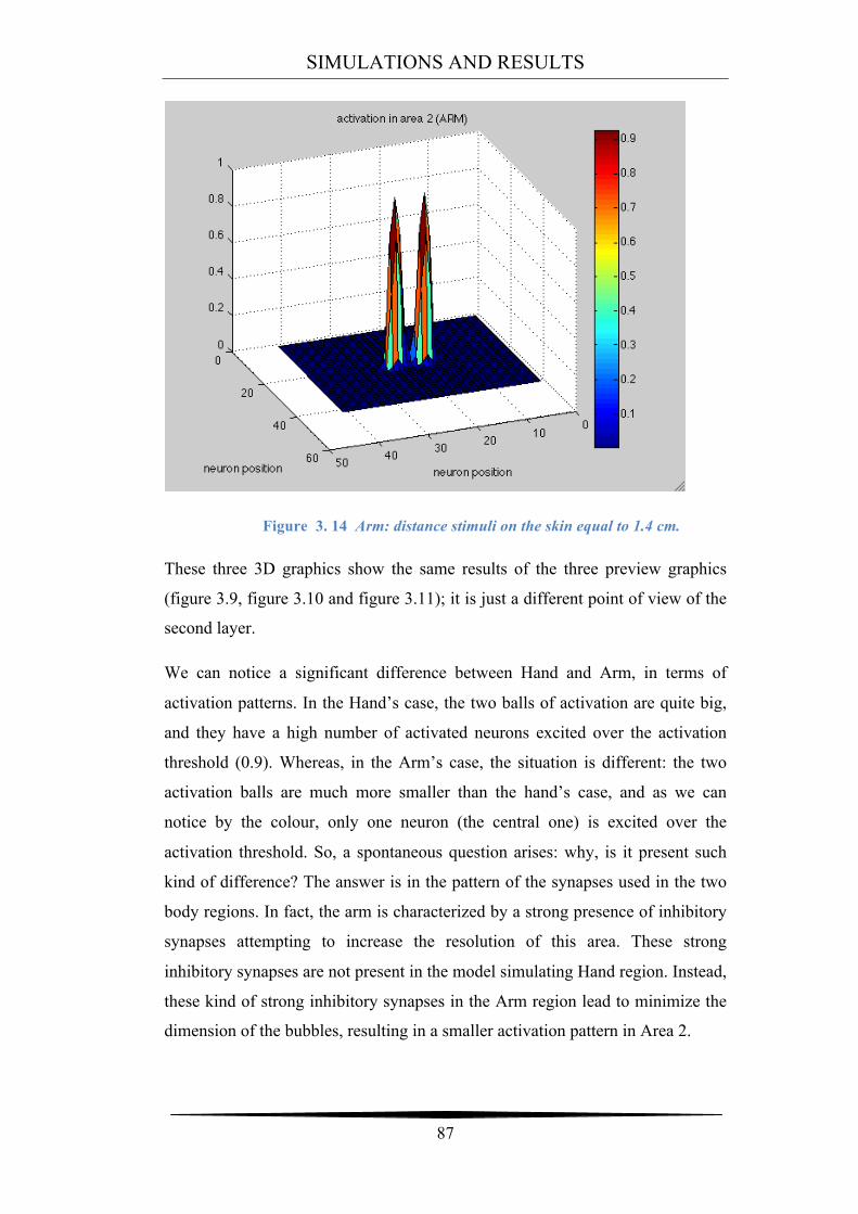
SIMULATIONS AND RESULTS
87
Figure 3. 14 Arm: distance stimuli on the skin equal to 1.4 cm.
These three 3D graphics show the same results of the three preview graphics
(figure 3.9, figure 3.10 and figure 3.11); it is just a different point of view of the
second layer.
We can notice a significant difference between Hand and Arm, in terms of
activation patterns. In the Hand’s case, the two balls of activation are quite big,
and they have a high number of activated neurons excited over the activation
threshold (0.9). Whereas, in the Arm’s case, the situation is different: the two
activation balls are much more smaller than the hand’s case, and as we can
notice by the colour, only one neuron (the central one) is excited over the
activation threshold. So, a spontaneous question arises: why, is it present such
kind of difference? The answer is in the pattern of the synapses used in the two
body regions. In fact, the arm is characterized by a strong presence of inhibitory
synapses attempting to increase the resolution of this area. These strong
inhibitory synapses are not present in the model simulating Hand region. Instead,
these kind of strong inhibitory synapses in the Arm region lead to minimize the
dimension of the bubbles, resulting in a smaller activation pattern in Area 2.
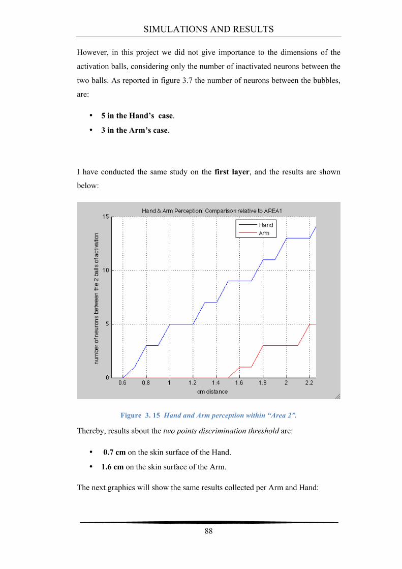
SIMULATIONS AND RESULTS
88
However, in this project we did not give importance to the dimensions of the
activation balls, considering only the number of inactivated neurons between the
two balls. As reported in figure 3.7 the number of neurons between the bubbles,
are:
• 5 in the Hand’s case.
• 3 in the Arm’s case.
I have conducted the same study on the first layer, and the results are shown
below:
Figure 3. 15 Hand and Arm perception within “Area 2”.
Thereby, results about the two points discrimination threshold are:
• 0.7 cm on the skin surface of the Hand.
• 1.6 cm on the skin surface of the Arm.
The next graphics will show the same results collected per Arm and Hand:
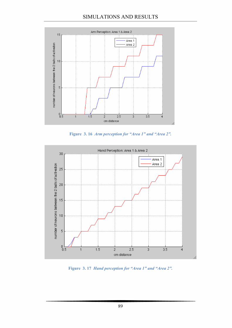
SIMULATIONS AND RESULTS
89
Figure 3. 16 Arm perception for “Area 1” and “Area 2”.
Figure 3. 17 Hand perception for “Area 1” and “Area 2”.
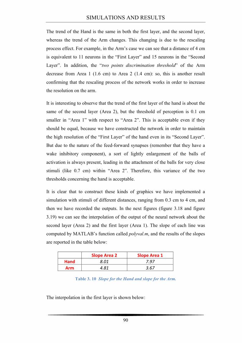
SIMULATIONS AND RESULTS
90
The trend of the Hand is the same in both the first layer, and the second layer,
whereas the trend of the Arm changes. This changing is due to the rescaling
process effect. For example, in the Arm’s case we can see that a distance of 4 cm
is equivalent to 11 neurons in the “First Layer” and 15 neurons in the “Second
Layer”. In addition, the “two points discrimination threshold” of the Arm
decrease from Area 1 (1.6 cm) to Area 2 (1.4 cm): so, this is another result
confirming that the rescaling process of the network works in order to increase
the resolution on the arm.
It is interesting to observe that the trend of the first layer of the hand is about the
same of the second layer (Area 2), but the threshold of perception is 0.1 cm
smaller in “Area 1” with respect to “Area 2”. This is acceptable even if they
should be equal, because we have constructed the network in order to maintain
the high resolution of the “First Layer” of the hand even in its “Second Layer”.
But due to the nature of the feed-forward synapses (remember that they have a
wake inhibitory component), a sort of lightly enlargement of the balls of
activation is always present, leading in the attachment of the balls for very close
stimuli (like 0.7 cm) within “Area 2”. Therefore, this variance of the two
thresholds concerning the hand is acceptable.
It is clear that to construct these kinds of graphics we have implemented a
simulation with stimuli of different distances, ranging from 0.3 cm to 4 cm, and
then we have recorded the outputs. In the next figures (figure 3.18 and figure
3.19) we can see the interpolation of the output of the neural network about the
second layer (Area 2) and the first layer (Area 1). The slope of each line was
computed by MATLAB’s function called polyval.m, and the results of the slopes
are reported in the table below:
Slope Area 2 Slope Area 1
Hand 8.01 7.97 Arm 4.81 3.67
Table 3. 10 Slope for the Hand and slope for the Arm.
The interpolation in the first layer is shown below:
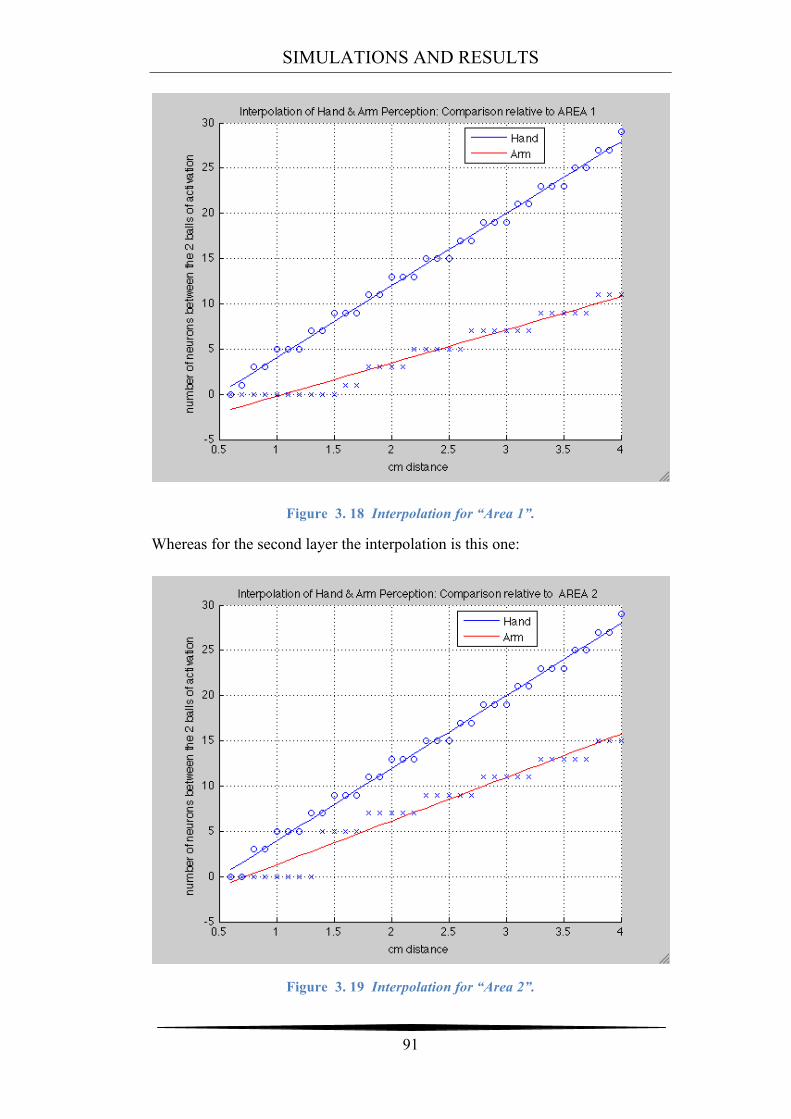
SIMULATIONS AND RESULTS
91
Figure 3. 18 Interpolation for “Area 1”.
Whereas for the second layer the interpolation is this one:
Figure 3. 19 Interpolation for “Area 2”.
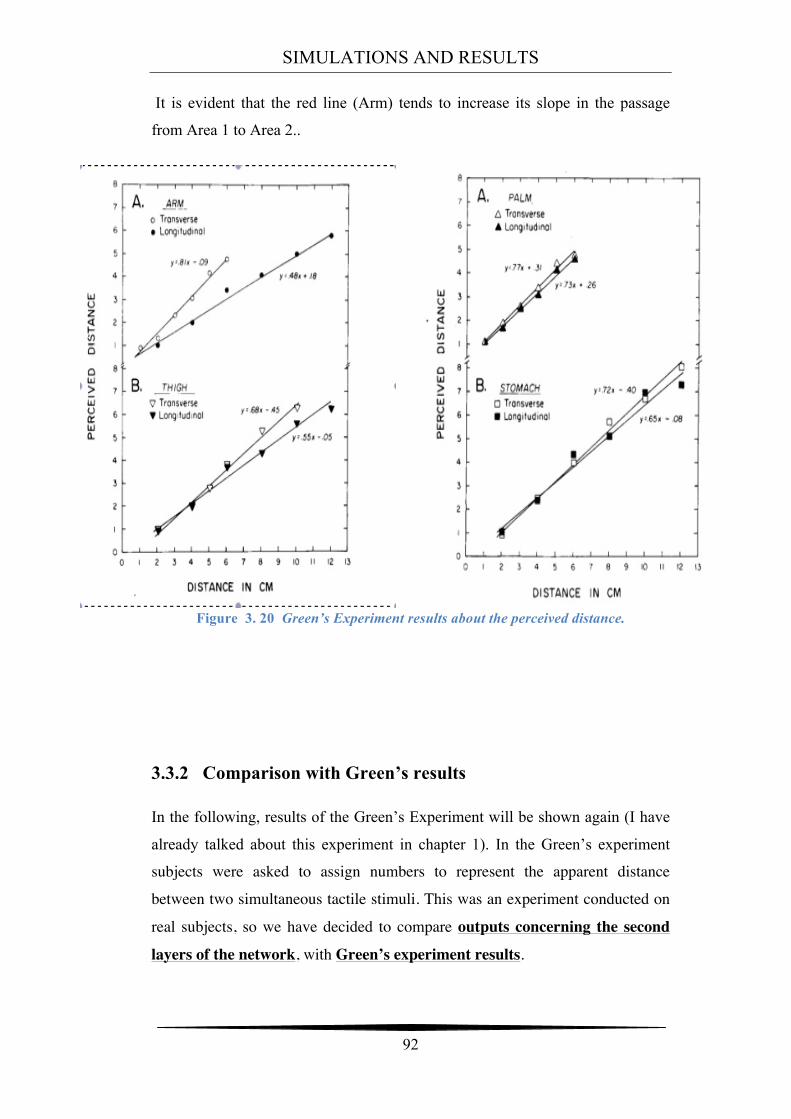
SIMULATIONS AND RESULTS
92
It is evident that the red line (Arm) tends to increase its slope in the passage
from Area 1 to Area 2..
Figure 3. 20 Green’s Experiment results about the perceived distance.
3.3.2 Comparison with Green’s results
In the following, results of the Green’s Experiment will be shown again (I have
already talked about this experiment in chapter 1). In the Green’s experiment
subjects were asked to assign numbers to represent the apparent distance
between two simultaneous tactile stimuli. This was an experiment conducted on
real subjects, so we have decided to compare outputs concerning the second
layers of the network, with Green’s experiment results.
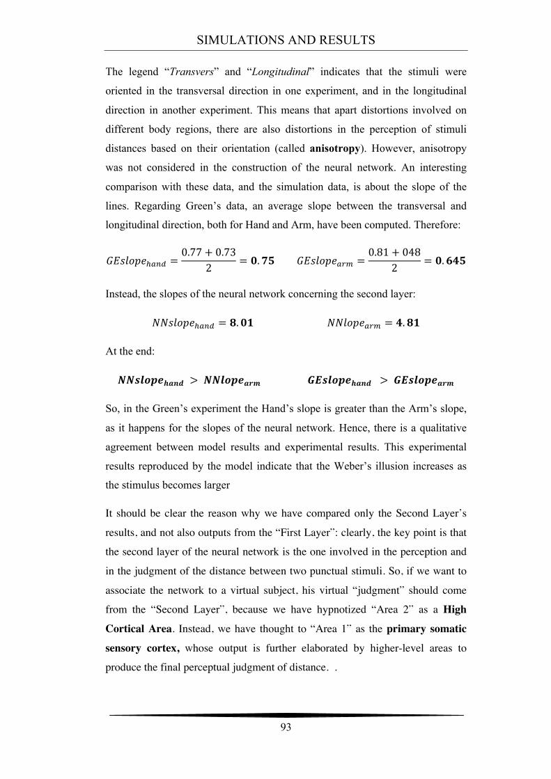
SIMULATIONS AND RESULTS
93
The legend “Transvers” and “Longitudinal” indicates that the stimuli were
oriented in the transversal direction in one experiment, and in the longitudinal
direction in another experiment. This means that apart distortions involved on
different body regions, there are also distortions in the perception of stimuli
distances based on their orientation (called anisotropy). However, anisotropy
was not considered in the construction of the neural network. An interesting
comparison with these data, and the simulation data, is about the slope of the
lines. Regarding Green’s data, an average slope between the transversal and
longitudinal direction, both for Hand and Arm, have been computed. Therefore:
!"#$%&!!!"# =0.77+ 0.73
2 = !.!" !"!"#$!!"# =0.81+ 048
2 = !.!"#
Instead, the slopes of the neural network concerning the second layer:
!!"#$%!!!"# = !.!" !!"#$!!"# = !.!"
At the end:
!!"#$%!!"#$ > !!"#$!!"# !"#$%&!!"#$ > !"!"#$!!"#
So, in the Green’s experiment the Hand’s slope is greater than the Arm’s slope,
as it happens for the slopes of the neural network. Hence, there is a qualitative
agreement between model results and experimental results. This experimental
results reproduced by the model indicate that the Weber’s illusion increases as
the stimulus becomes larger
It should be clear the reason why we have compared only the Second Layer’s
results, and not also outputs from the “First Layer”: clearly, the key point is that
the second layer of the neural network is the one involved in the perception and
in the judgment of the distance between two punctual stimuli. So, if we want to
associate the network to a virtual subject, his virtual “judgment” should come
from the “Second Layer”, because we have hypnotized “Area 2” as a High
Cortical Area. Instead, we have thought to “Area 1” as the primary somatic
sensory cortex, whose output is further elaborated by higher-level areas to
produce the final perceptual judgment of distance. .
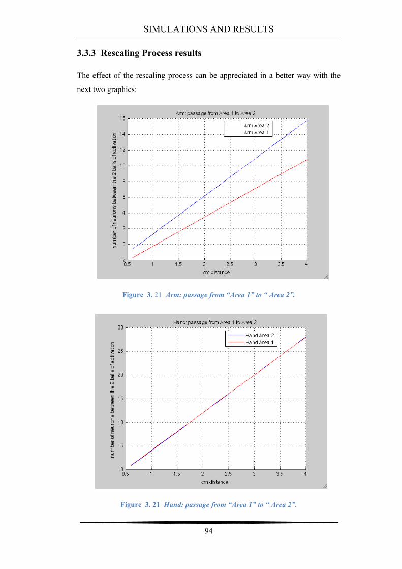
SIMULATIONS AND RESULTS
94
3.3.3 Rescaling Process results
The effect of the rescaling process can be appreciated in a better way with the
next two graphics:
Figure 3. 21 Arm: passage from “Area 1” to “ Area 2”.
Figure 3. 21 Hand: passage from “Area 1” to “ Area 2”.
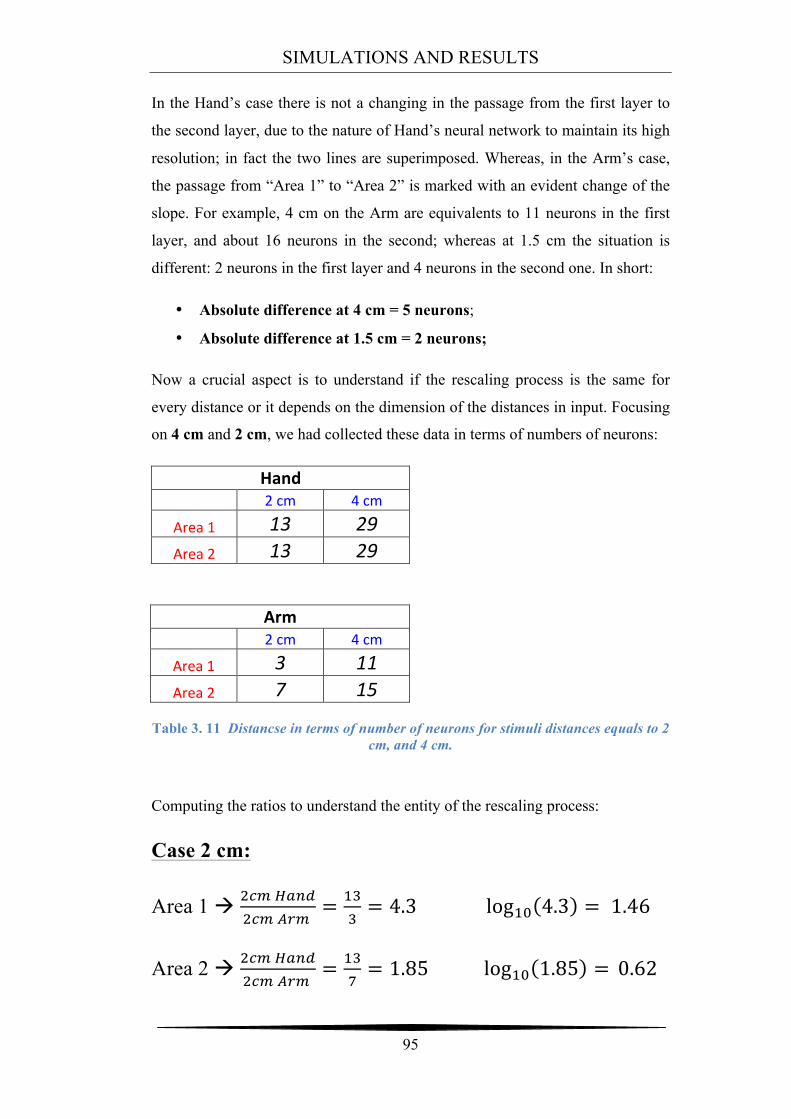
SIMULATIONS AND RESULTS
95
In the Hand’s case there is not a changing in the passage from the first layer to
the second layer, due to the nature of Hand’s neural network to maintain its high
resolution; in fact the two lines are superimposed. Whereas, in the Arm’s case,
the passage from “Area 1” to “Area 2” is marked with an evident change of the
slope. For example, 4 cm on the Arm are equivalents to 11 neurons in the first
layer, and about 16 neurons in the second; whereas at 1.5 cm the situation is
different: 2 neurons in the first layer and 4 neurons in the second one. In short:
• Absolute difference at 4 cm = 5 neurons;
• Absolute difference at 1.5 cm = 2 neurons;
Now a crucial aspect is to understand if the rescaling process is the same for
every distance or it depends on the dimension of the distances in input. Focusing
on 4 cm and 2 cm, we had collected these data in terms of numbers of neurons:
Hand 2 cm 4 cm
Area 1 13 29 Area 2 13 29
Arm 2 cm 4 cm
Area 1 3 11 Area 2 7 15
Table 3. 11 Distancse in terms of number of neurons for stimuli distances equals to 2
cm, and 4 cm.
Computing the ratios to understand the entity of the rescaling process:
Case 2 cm:
Area 1 à !!" !"#$!!" !"#
= !"!= 4.3 log!" 4.3 = 1.46
Area 2 à !!" !"#$!!" !"#
= !"!= 1.85 log!" 1.85 = 0.62
SIMULATIONS AND RESULTS
96
Case 4cm:
Area 1 à !!" !"#$!!" !"#
= !"!!= 2.63 log!" 2.63 = 0.97
Area 2 à !!" !"#$!!" !"#
= !"!"= 1.93 log!" 1.93 = 0.65
Case 2cm Case 4cm Absolute difference between “ratio
Area 1” and “ratio Area 2” 2.98 0.7 Absolute difference between log
“ratio Area 1” and “log ratio Area” 2 0.84 0.32
Table 3. 12 Entity of the Rescaling.
In each case the ratio tends to decrease due to the presence of the rescaling
process, but the entity of the decrement is different: it is greater in case of 2 cm
than case of 4 cm. Thereby, in base on the neural network’s results, we can
assert that the rescaling process is strongest for small distances, and it is weak
for big distances. So there is an inverse proportion between the distances and
the entity of the Rescaling. At the same time, going back to the Green’s
Experiment results (figure 3.20), we can see that for big distances the Weber’s
Illusion tends to increase due to the different slope of the Hand and the Arm: in
particular the Hand’s slope is higher than the Arm’s slope, hence the two lines
will diverge for big distances.
A possible explanation of the Illusion Increment might be given by these results,
because, the point is that for big distances the “Rescaling Process” is going to
become weak, allowing an increment of the Weber’s Illusion. Hereby, we do not
want to assert that this is the real reason for the increment of the Weber’s
Illusion, even because there are not experimental evidences to validate this
theory. However, the neural network gives in output these kinds of results, and
this theory seems congruent to explaining the Illusion Increment.
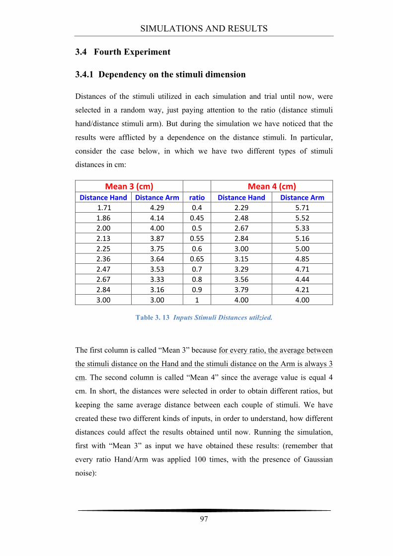
SIMULATIONS AND RESULTS
97
3.4 Fourth Experiment
3.4.1 Dependency on the stimuli dimension
Distances of the stimuli utilized in each simulation and trial until now, were
selected in a random way, just paying attention to the ratio (distance stimuli
hand/distance stimuli arm). But during the simulation we have noticed that the
results were afflicted by a dependence on the distance stimuli. In particular,
consider the case below, in which we have two different types of stimuli
distances in cm:
Mean 3 (cm) Mean 4 (cm) Distance Hand Distance Arm ratio Distance Hand Distance Arm
1.71 4.29 0.4 2.29 5.71 1.86 4.14 0.45 2.48 5.52 2.00 4.00 0.5 2.67 5.33 2.13 3.87 0.55 2.84 5.16 2.25 3.75 0.6 3.00 5.00 2.36 3.64 0.65 3.15 4.85 2.47 3.53 0.7 3.29 4.71 2.67 3.33 0.8 3.56 4.44 2.84 3.16 0.9 3.79 4.21 3.00 3.00 1 4.00 4.00
Table 3. 13 Inputs Stimuli Distances utilzied.
The first column is called “Mean 3” because for every ratio, the average between
the stimuli distance on the Hand and the stimuli distance on the Arm is always 3
cm. The second column is called “Mean 4” since the average value is equal 4
cm. In short, the distances were selected in order to obtain different ratios, but
keeping the same average distance between each couple of stimuli. We have
created these two different kinds of inputs, in order to understand, how different
distances could affect the results obtained until now. Running the simulation,
first with “Mean 3” as input we have obtained these results: (remember that
every ratio Hand/Arm was applied 100 times, with the presence of Gaussian
noise):
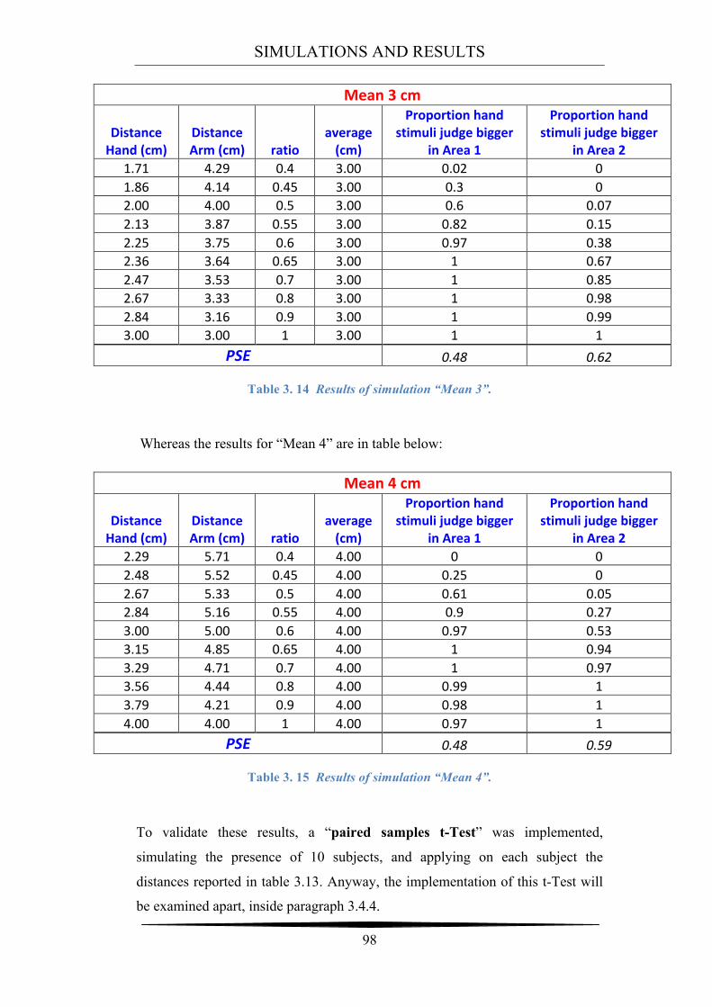
SIMULATIONS AND RESULTS
98
Mean 3 cm
Distance Hand (cm)
Distance Arm (cm) ratio
average (cm)
Proportion hand stimuli judge bigger
in Area 1
Proportion hand stimuli judge bigger
in Area 2 1.71 4.29 0.4 3.00 0.02 0 1.86 4.14 0.45 3.00 0.3 0 2.00 4.00 0.5 3.00 0.6 0.07 2.13 3.87 0.55 3.00 0.82 0.15 2.25 3.75 0.6 3.00 0.97 0.38 2.36 3.64 0.65 3.00 1 0.67 2.47 3.53 0.7 3.00 1 0.85 2.67 3.33 0.8 3.00 1 0.98 2.84 3.16 0.9 3.00 1 0.99 3.00 3.00 1 3.00 1 1
PSE 0.48 0.62
Table 3. 14 Results of simulation “Mean 3”.
Whereas the results for “Mean 4” are in table below:
Mean 4 cm
Distance Hand (cm)
Distance Arm (cm) ratio
average (cm)
Proportion hand stimuli judge bigger
in Area 1
Proportion hand stimuli judge bigger
in Area 2 2.29 5.71 0.4 4.00 0 0 2.48 5.52 0.45 4.00 0.25 0 2.67 5.33 0.5 4.00 0.61 0.05 2.84 5.16 0.55 4.00 0.9 0.27 3.00 5.00 0.6 4.00 0.97 0.53 3.15 4.85 0.65 4.00 1 0.94 3.29 4.71 0.7 4.00 1 0.97 3.56 4.44 0.8 4.00 0.99 1 3.79 4.21 0.9 4.00 0.98 1 4.00 4.00 1 4.00 0.97 1
PSE 0.48 0.59
Table 3. 15 Results of simulation “Mean 4”.
To validate these results, a “paired samples t-Test” was implemented,
simulating the presence of 10 subjects, and applying on each subject the
distances reported in table 3.13. Anyway, the implementation of this t-Test will
be examined apart, inside paragraph 3.4.4.
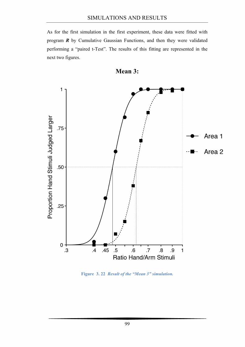
SIMULATIONS AND RESULTS
99
As for the first simulation in the first experiment, these data were fitted with
program R by Cumulative Gaussian Functions, and then they were validated
performing a “paired t-Test”. The results of this fitting are represented in the
next two figures.
Mean 3:
Figure 3. 22 Result of the “Mean 3” simulation.
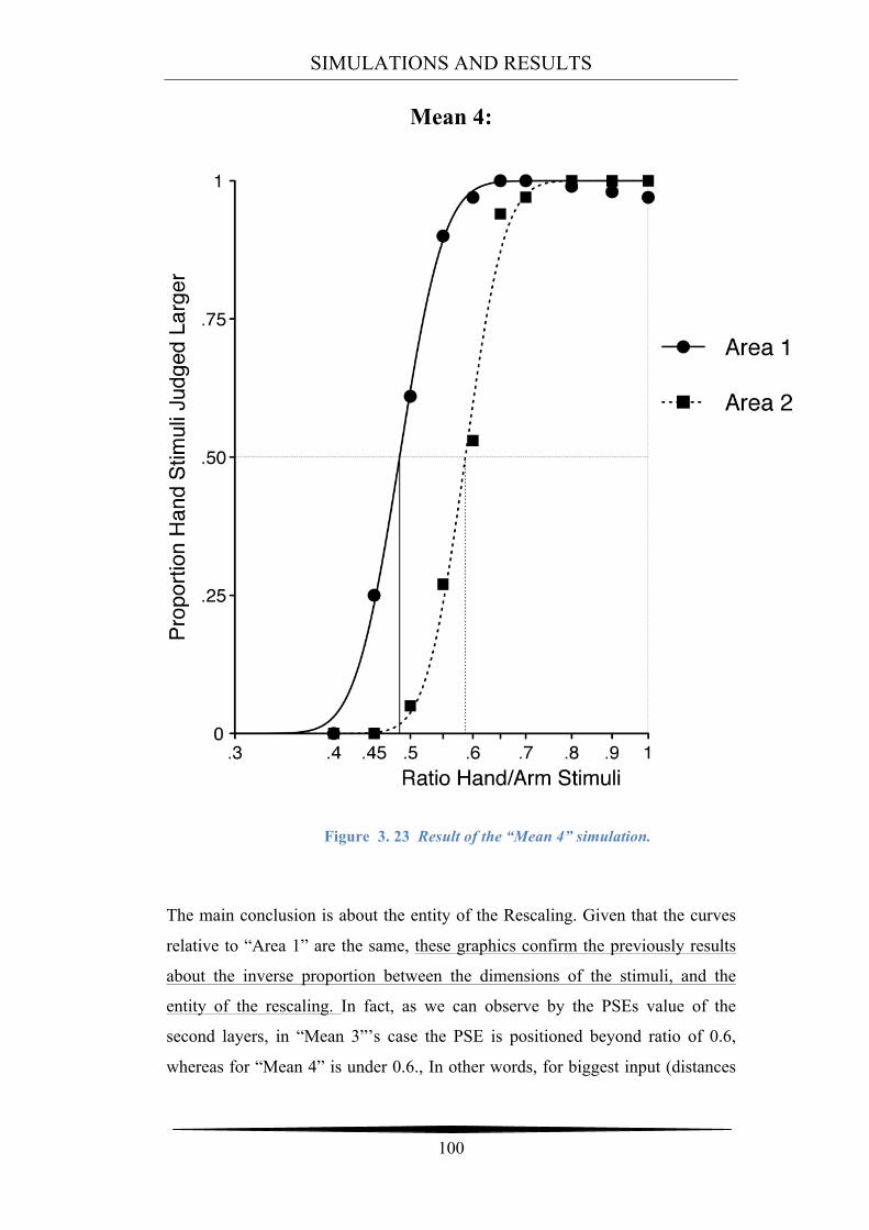
SIMULATIONS AND RESULTS
100
Mean 4:
Figure 3. 23 Result of the “Mean 4” simulation.
The main conclusion is about the entity of the Rescaling. Given that the curves
relative to “Area 1” are the same, these graphics confirm the previously results
about the inverse proportion between the dimensions of the stimuli, and the
entity of the rescaling. In fact, as we can observe by the PSEs value of the
second layers, in “Mean 3”’s case the PSE is positioned beyond ratio of 0.6,
whereas for “Mean 4” is under 0.6., In other words, for biggest input (distances
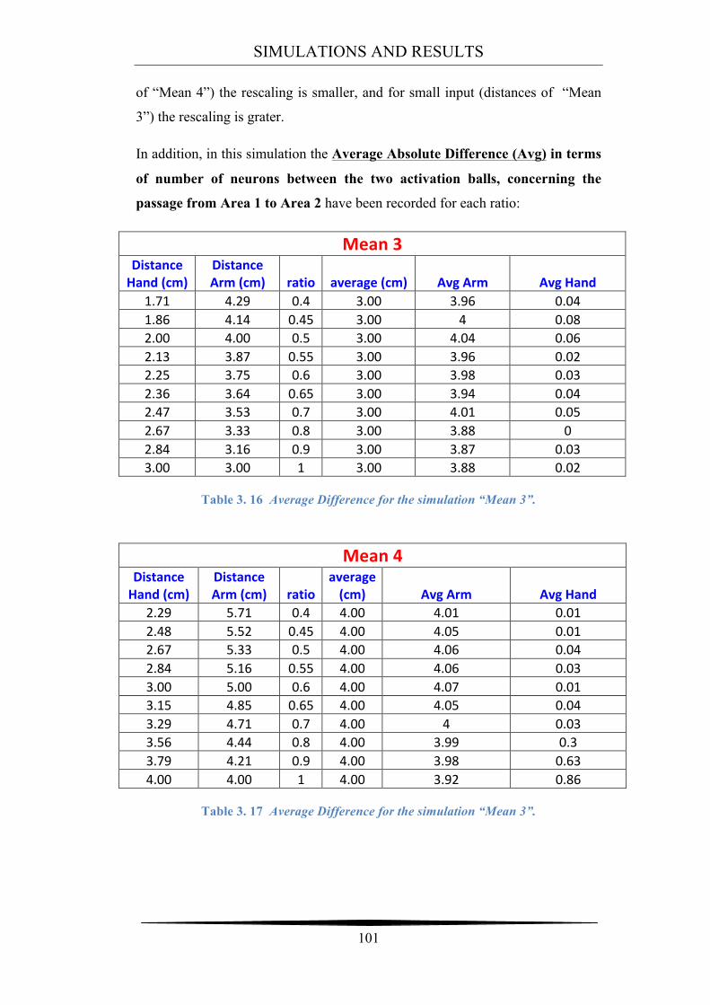
SIMULATIONS AND RESULTS
101
of “Mean 4”) the rescaling is smaller, and for small input (distances of “Mean
3”) the rescaling is grater.
In addition, in this simulation the Average Absolute Difference (Avg) in terms
of number of neurons between the two activation balls, concerning the
passage from Area 1 to Area 2 have been recorded for each ratio:
Mean 3 Distance Hand (cm)
Distance Arm (cm) ratio average (cm) Avg Arm Avg Hand
1.71 4.29 0.4 3.00 3.96 0.04 1.86 4.14 0.45 3.00 4 0.08 2.00 4.00 0.5 3.00 4.04 0.06 2.13 3.87 0.55 3.00 3.96 0.02 2.25 3.75 0.6 3.00 3.98 0.03 2.36 3.64 0.65 3.00 3.94 0.04 2.47 3.53 0.7 3.00 4.01 0.05 2.67 3.33 0.8 3.00 3.88 0 2.84 3.16 0.9 3.00 3.87 0.03 3.00 3.00 1 3.00 3.88 0.02
Table 3. 16 Average Difference for the simulation “Mean 3”.
Mean 4 Distance Hand (cm)
Distance Arm (cm) ratio
average (cm) Avg Arm Avg Hand
2.29 5.71 0.4 4.00 4.01 0.01 2.48 5.52 0.45 4.00 4.05 0.01 2.67 5.33 0.5 4.00 4.06 0.04 2.84 5.16 0.55 4.00 4.06 0.03 3.00 5.00 0.6 4.00 4.07 0.01 3.15 4.85 0.65 4.00 4.05 0.04 3.29 4.71 0.7 4.00 4 0.03 3.56 4.44 0.8 4.00 3.99 0.3 3.79 4.21 0.9 4.00 3.98 0.63 4.00 4.00 1 4.00 3.92 0.86
Table 3. 17 Average Difference for the simulation “Mean 3”.
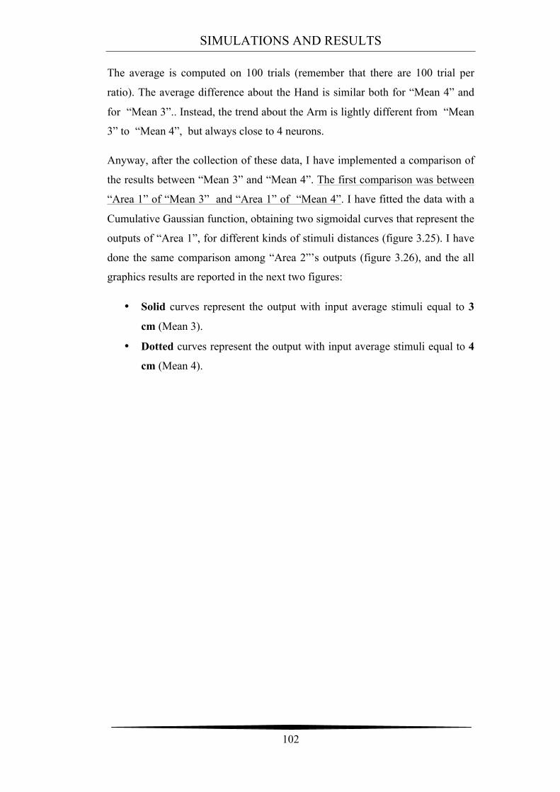
SIMULATIONS AND RESULTS
102
The average is computed on 100 trials (remember that there are 100 trial per
ratio). The average difference about the Hand is similar both for “Mean 4” and
for “Mean 3”.. Instead, the trend about the Arm is lightly different from “Mean
3” to “Mean 4”, but always close to 4 neurons.
Anyway, after the collection of these data, I have implemented a comparison of
the results between “Mean 3” and “Mean 4”. The first comparison was between
“Area 1” of “Mean 3” and “Area 1” of “Mean 4”. I have fitted the data with a
Cumulative Gaussian function, obtaining two sigmoidal curves that represent the
outputs of “Area 1”, for different kinds of stimuli distances (figure 3.25). I have
done the same comparison among “Area 2”’s outputs (figure 3.26), and the all
graphics results are reported in the next two figures:
• Solid curves represent the output with input average stimuli equal to 3
cm (Mean 3).
• Dotted curves represent the output with input average stimuli equal to 4
cm (Mean 4).
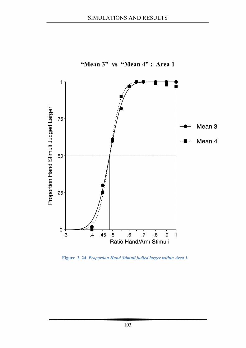
SIMULATIONS AND RESULTS
103
“Mean 3” vs “Mean 4” : Area 1
Figure 3. 24 Proportion Hand Stimuli judjed larger within Area 1.
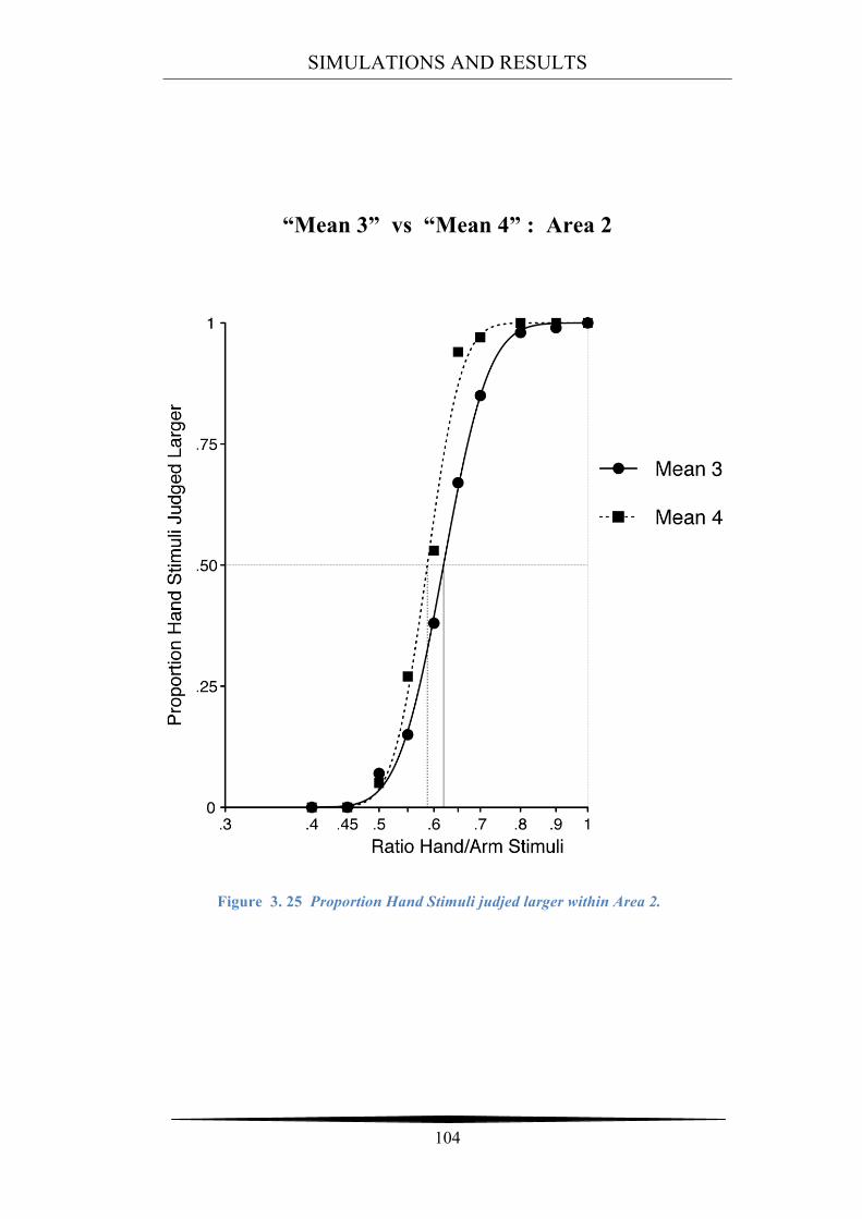
SIMULATIONS AND RESULTS
104
“Mean 3” vs “Mean 4” : Area 2
Figure 3. 25 Proportion Hand Stimuli judjed larger within Area 2.
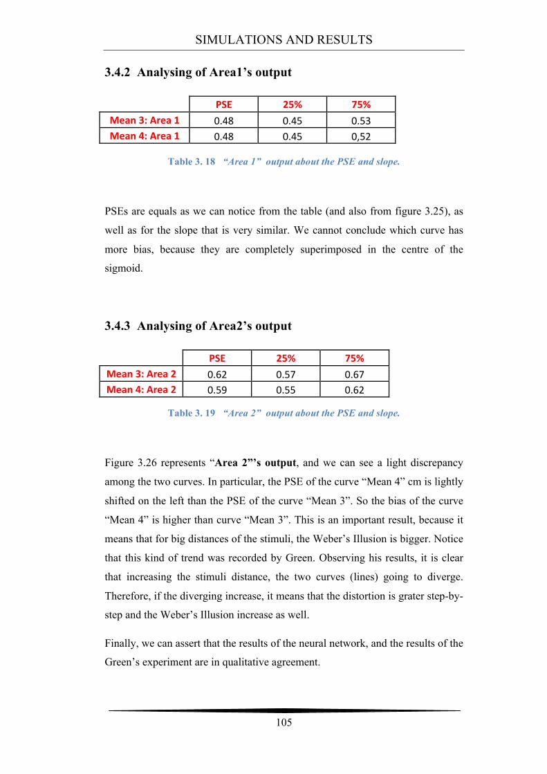
SIMULATIONS AND RESULTS
105
3.4.2 Analysing of Area1’s output
PSE 25% 75%
Mean 3: Area 1 0.48 0.45 0.53 Mean 4: Area 1 0.48 0.45 0,52
Table 3. 18 “Area 1” output about the PSE and slope.
PSEs are equals as we can notice from the table (and also from figure 3.25), as
well as for the slope that is very similar. We cannot conclude which curve has
more bias, because they are completely superimposed in the centre of the
sigmoid.
3.4.3 Analysing of Area2’s output
PSE 25% 75%
Mean 3: Area 2 0.62 0.57 0.67 Mean 4: Area 2 0.59 0.55 0.62
Table 3. 19 “Area 2” output about the PSE and slope.
Figure 3.26 represents “Area 2”’s output, and we can see a light discrepancy
among the two curves. In particular, the PSE of the curve “Mean 4” cm is lightly
shifted on the left than the PSE of the curve “Mean 3”. So the bias of the curve
“Mean 4” is higher than curve “Mean 3”. This is an important result, because it
means that for big distances of the stimuli, the Weber’s Illusion is bigger. Notice
that this kind of trend was recorded by Green. Observing his results, it is clear
that increasing the stimuli distance, the two curves (lines) going to diverge.
Therefore, if the diverging increase, it means that the distortion is grater step-by-
step and the Weber’s Illusion increase as well.
Finally, we can assert that the results of the neural network, and the results of the
Green’s experiment are in qualitative agreement.
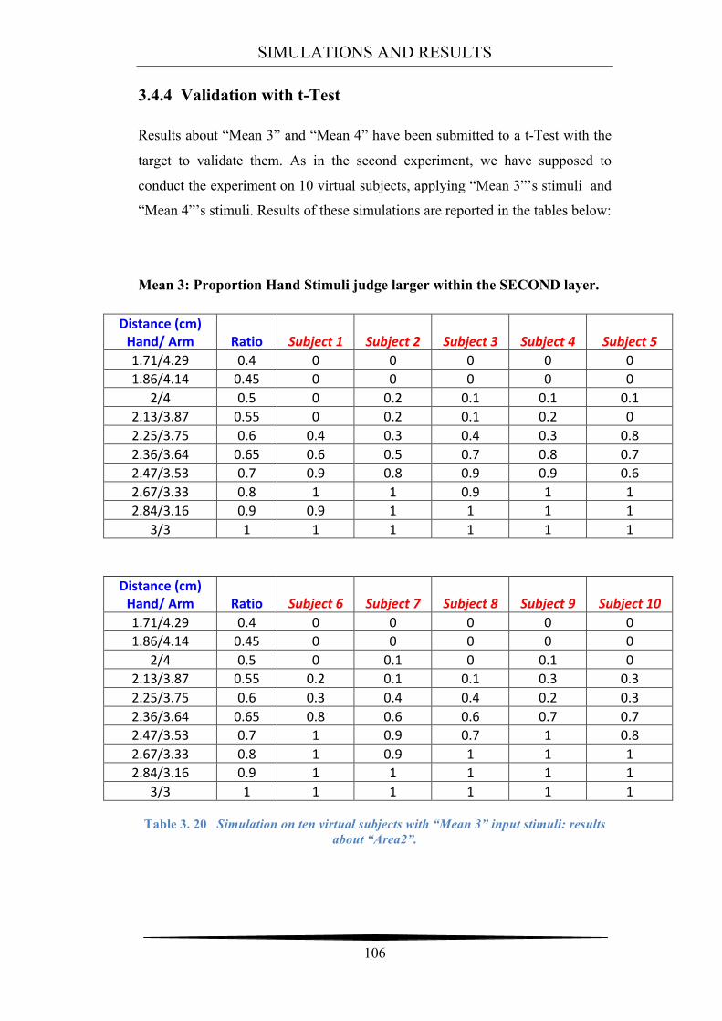
SIMULATIONS AND RESULTS
106
3.4.4 Validation with t-Test
Results about “Mean 3” and “Mean 4” have been submitted to a t-Test with the
target to validate them. As in the second experiment, we have supposed to
conduct the experiment on 10 virtual subjects, applying “Mean 3”’s stimuli and
“Mean 4”’s stimuli. Results of these simulations are reported in the tables below:
Mean 3: Proportion Hand Stimuli judge larger within the SECOND layer.
Distance (cm) Hand/ Arm Ratio Subject 1 Subject 2 Subject 3 Subject 4 Subject 5 1.71/4.29 0.4 0 0 0 0 0 1.86/4.14 0.45 0 0 0 0 0
2/4 0.5 0 0.2 0.1 0.1 0.1 2.13/3.87 0.55 0 0.2 0.1 0.2 0 2.25/3.75 0.6 0.4 0.3 0.4 0.3 0.8 2.36/3.64 0.65 0.6 0.5 0.7 0.8 0.7 2.47/3.53 0.7 0.9 0.8 0.9 0.9 0.6 2.67/3.33 0.8 1 1 0.9 1 1 2.84/3.16 0.9 0.9 1 1 1 1
3/3 1 1 1 1 1 1
Distance (cm) Hand/ Arm Ratio Subject 6 Subject 7 Subject 8 Subject 9 Subject 10 1.71/4.29 0.4 0 0 0 0 0 1.86/4.14 0.45 0 0 0 0 0
2/4 0.5 0 0.1 0 0.1 0 2.13/3.87 0.55 0.2 0.1 0.1 0.3 0.3 2.25/3.75 0.6 0.3 0.4 0.4 0.2 0.3 2.36/3.64 0.65 0.8 0.6 0.6 0.7 0.7 2.47/3.53 0.7 1 0.9 0.7 1 0.8 2.67/3.33 0.8 1 0.9 1 1 1 2.84/3.16 0.9 1 1 1 1 1
3/3 1 1 1 1 1 1
Table 3. 20 Simulation on ten virtual subjects with “Mean 3” input stimuli: results about “Area2”.
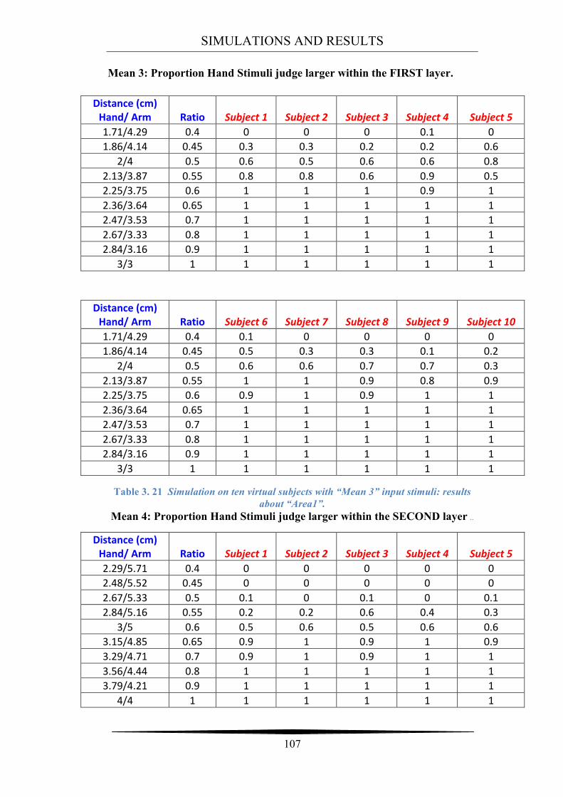
SIMULATIONS AND RESULTS
107
Mean 3: Proportion Hand Stimuli judge larger within the FIRST layer.
Distance (cm) Hand/ Arm Ratio Subject 1 Subject 2 Subject 3 Subject 4 Subject 5 1.71/4.29 0.4 0 0 0 0.1 0 1.86/4.14 0.45 0.3 0.3 0.2 0.2 0.6
2/4 0.5 0.6 0.5 0.6 0.6 0.8 2.13/3.87 0.55 0.8 0.8 0.6 0.9 0.5 2.25/3.75 0.6 1 1 1 0.9 1 2.36/3.64 0.65 1 1 1 1 1 2.47/3.53 0.7 1 1 1 1 1 2.67/3.33 0.8 1 1 1 1 1 2.84/3.16 0.9 1 1 1 1 1
3/3 1 1 1 1 1 1
Distance (cm) Hand/ Arm Ratio Subject 6 Subject 7 Subject 8 Subject 9 Subject 10 1.71/4.29 0.4 0.1 0 0 0 0 1.86/4.14 0.45 0.5 0.3 0.3 0.1 0.2
2/4 0.5 0.6 0.6 0.7 0.7 0.3 2.13/3.87 0.55 1 1 0.9 0.8 0.9 2.25/3.75 0.6 0.9 1 0.9 1 1 2.36/3.64 0.65 1 1 1 1 1 2.47/3.53 0.7 1 1 1 1 1 2.67/3.33 0.8 1 1 1 1 1 2.84/3.16 0.9 1 1 1 1 1
3/3 1 1 1 1 1 1
Table 3. 21 Simulation on ten virtual subjects with “Mean 3” input stimuli: results about “Area1”.
Mean 4: Proportion Hand Stimuli judge larger within the SECOND layer ..
Distance (cm) Hand/ Arm Ratio Subject 1 Subject 2 Subject 3 Subject 4 Subject 5 2.29/5.71 0.4 0 0 0 0 0 2.48/5.52 0.45 0 0 0 0 0 2.67/5.33 0.5 0.1 0 0.1 0 0.1 2.84/5.16 0.55 0.2 0.2 0.6 0.4 0.3
3/5 0.6 0.5 0.6 0.5 0.6 0.6 3.15/4.85 0.65 0.9 1 0.9 1 0.9 3.29/4.71 0.7 0.9 1 0.9 1 1 3.56/4.44 0.8 1 1 1 1 1 3.79/4.21 0.9 1 1 1 1 1
4/4 1 1 1 1 1 1
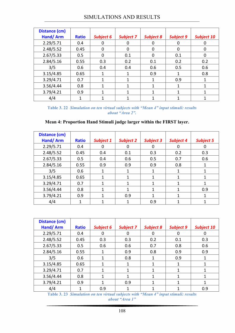
SIMULATIONS AND RESULTS
108
Distance (cm) Hand/ Arm Ratio Subject 6 Subject 7 Subject 8 Subject 9 Subject 10 2.29/5.71 0.4 0 0 0 0 0 2.48/5.52 0.45 0 0 0 0 0 2.67/5.33 0.5 0 0.1 0 0.1 0 2.84/5.16 0.55 0.3 0.2 0.1 0.2 0.2
3/5 0.6 0.4 0.4 0.6 0.5 0.6 3.15/4.85 0.65 1 1 0.9 1 0.8 3.29/4.71 0.7 1 1 1 0.9 1 3.56/4.44 0.8 1 1 1 1 1 3.79/4.21 0.9 1 1 1 1 1
4/4 1 1 1 1 1 1
Table 3. 22 Simulation on ten virtual subjects with “Mean 4” input stimuli: results about “Area 2”.
Mean 4: Proportion Hand Stimuli judge larger within the FIRST layer.
Distance (cm) Hand/ Arm Ratio Subject 1 Subject 2 Subject 3 Subject 4 Subject 5 2.29/5.71 0.4 0 0 0 0 0 2.48/5.52 0.45 0.4 0.1 0.3 0.2 0.3 2.67/5.33 0.5 0.4 0.6 0.5 0.7 0.6 2.84/5.16 0.55 0.9 0.9 0.9 0.8 1
3/5 0.6 1 1 1 1 1 3.15/4.85 0.65 1 1 1 1 1 3.29/4.71 0.7 1 1 1 1 1 3.56/4.44 0.8 1 1 1 1 0.9 3.79/4.21 0.9 1 0.9 1 1 1
4/4 1 1 1 0.9 1 1
Distance (cm) Hand/ Arm Ratio Subject 6 Subject 7 Subject 8 Subject 9 Subject 10 2.29/5.71 0.4 0 0 0 0 0 2.48/5.52 0.45 0.3 0.3 0.2 0.1 0.3 2.67/5.33 0.5 0.6 0.6 0.7 0.8 0.6 2.84/5.16 0.55 1 0.9 0.8 0.9 0.9
3/5 0.6 1 0.8 1 0.9 1 3.15/4.85 0.65 1 1 1 1 1 3.29/4.71 0.7 1 1 1 1 1 3.56/4.44 0.8 1 1 1 1 1 3.79/4.21 0.9 1 0.9 1 1 1
4/4 1 0.9 1 1 1 0.9 Table 3. 23 Simulation on ten virtual subjects with “Mean 4” input stimuli: results
about “Area 1”
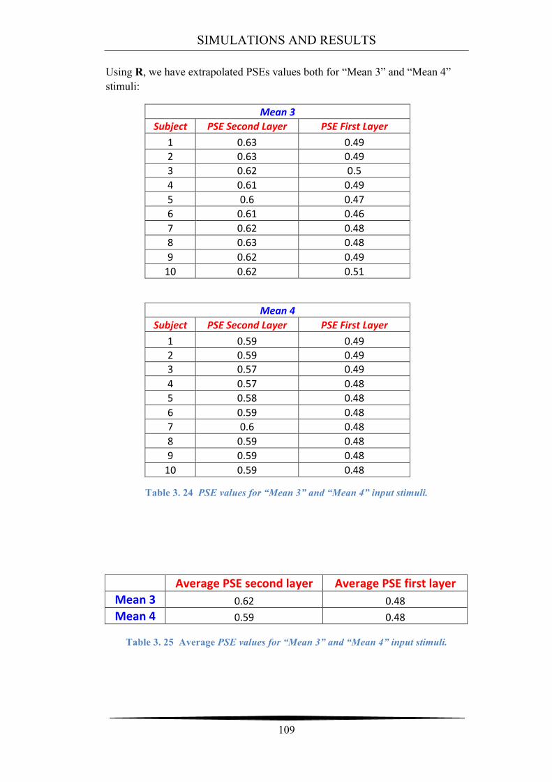
SIMULATIONS AND RESULTS
109
Using R, we have extrapolated PSEs values both for “Mean 3” and “Mean 4” stimuli:
Mean 3 Subject PSE Second Layer PSE First Layer
1 0.63 0.49 2 0.63 0.49 3 0.62 0.5 4 0.61 0.49 5 0.6 0.47 6 0.61 0.46 7 0.62 0.48 8 0.63 0.48 9 0.62 0.49 10 0.62 0.51
Mean 4 Subject PSE Second Layer PSE First Layer
1 0.59 0.49 2 0.59 0.49 3 0.57 0.49 4 0.57 0.48 5 0.58 0.48 6 0.59 0.48 7 0.6 0.48 8 0.59 0.48 9 0.59 0.48 10 0.59 0.48
Table 3. 24 PSE values for “Mean 3” and “Mean 4” input stimuli.
Average PSE second layer Average PSE first layer
Mean 3 0.62 0.48 Mean 4 0.59 0.48
Table 3. 25 Average PSE values for “Mean 3” and “Mean 4” input stimuli.
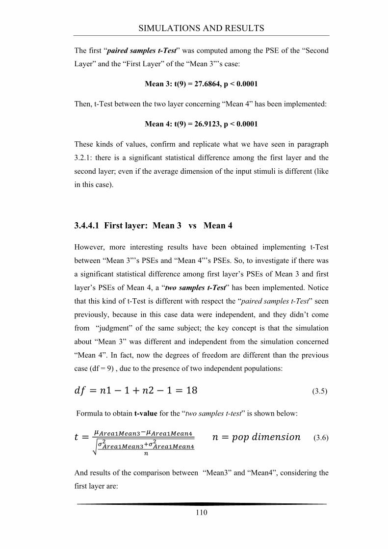
SIMULATIONS AND RESULTS
110
The first “paired samples t-Test” was computed among the PSE of the “Second
Layer” and the “First Layer” of the “Mean 3”’s case:
Mean 3: t(9) = 27.6864, p < 0.0001
Then, t-Test between the two layer concerning “Mean 4” has been implemented:
Mean 4: t(9) = 26.9123, p < 0.0001
These kinds of values, confirm and replicate what we have seen in paragraph
3.2.1: there is a significant statistical difference among the first layer and the
second layer; even if the average dimension of the input stimuli is different (like
in this case).
3.4.4.1 First layer: Mean 3 vs Mean 4
However, more interesting results have been obtained implementing t-Test
between “Mean 3”’s PSEs and “Mean 4”’s PSEs. So, to investigate if there was
a significant statistical difference among first layer’s PSEs of Mean 3 and first
layer’s PSEs of Mean 4, a “two samples t-Test” has been implemented. Notice
that this kind of t-Test is different with respect the “paired samples t-Test” seen
previously, because in this case data were independent, and they didn’t come
from “judgment” of the same subject; the key concept is that the simulation
about “Mean 3” was different and independent from the simulation concerned
“Mean 4”. In fact, now the degrees of freedom are different than the previous
case (df = 9) , due to the presence of two independent populations:
!" = !1 − 1 + !2 − 1 = 18 (3.5)
Formula to obtain t-value for the “two samples t-test” is shown below:
! = !!"#$!!"#$!!!!"#$!!"#$!
!!"#$!!"#$!! !!!"#$!!"#$!
!
!
! = !"! !"#$%&"'% (3.6)
And results of the comparison between “Mean3” and “Mean4”, considering the
first layer are:
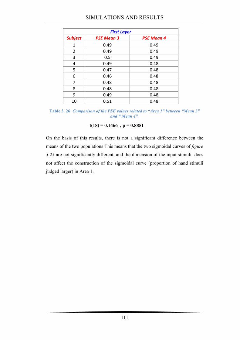
SIMULATIONS AND RESULTS
111
First Layer Subject PSE Mean 3 PSE Mean 4
1 0.49 0.49 2 0.49 0.49 3 0.5 0.49 4 0.49 0.48 5 0.47 0.48 6 0.46 0.48 7 0.48 0.48 8 0.48 0.48 9 0.49 0.48 10 0.51 0.48
Table 3. 26 Comparison of the PSE values related to “Area 1” between “Mean 3”
and “ Mean 4”.
t(18) = 0.1466 , p = 0.8851
On the basis of this results, there is not a significant difference between the
means of the two populations This means that the two sigmoidal curves of figure
3.25 are not significantly different, and the dimension of the input stimuli does
not affect the construction of the sigmoidal curve (proportion of hand stimuli
judged larger) in Area 1.
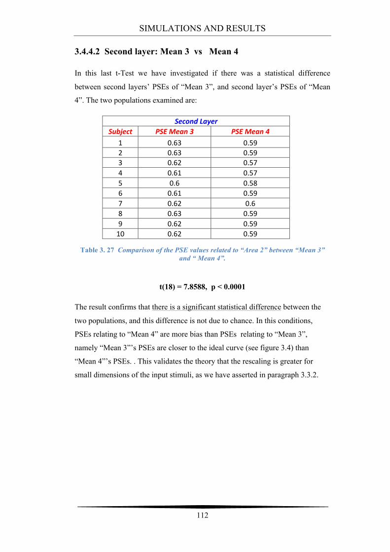
SIMULATIONS AND RESULTS
112
3.4.4.2 Second layer: Mean 3 vs Mean 4
In this last t-Test we have investigated if there was a statistical difference
between second layers’ PSEs of “Mean 3”, and second layer’s PSEs of “Mean
4”. The two populations examined are:
Second Layer Subject PSE Mean 3 PSE Mean 4
1 0.63 0.59 2 0.63 0.59 3 0.62 0.57 4 0.61 0.57 5 0.6 0.58 6 0.61 0.59 7 0.62 0.6 8 0.63 0.59 9 0.62 0.59 10 0.62 0.59
Table 3. 27 Comparison of the PSE values related to “Area 2” between “Mean 3”
and “ Mean 4”.
t(18) = 7.8588, p < 0.0001
The result confirms that there is a significant statistical difference between the
two populations, and this difference is not due to chance. In this conditions,
PSEs relating to “Mean 4” are more bias than PSEs relating to “Mean 3”,
namely “Mean 3”’s PSEs are closer to the ideal curve (see figure 3.4) than
“Mean 4”’s PSEs. . This validates the theory that the rescaling is greater for
small dimensions of the input stimuli, as we have asserted in paragraph 3.3.2.
113
Chapter 4
PARAMETER SENSITIVITY ANALYSIS
4.1 Parameter Sensitivity Analysis and Reference Results
This kind of analysis has the purpose of investigating the behaviour of the neural
network changing parameters one by one. In short, we have conducted different
simulations, in each simulation changing the value of just one parameter at a
time with respect to the reference value reported in table 4.1.
The changing of some kinds of parameters might leads to a dramatically change
of the network outputs, whereas, other parameters could not change substantially
the behaviour of the network. Hence, it is clear that this study was very
important to understand which parameters influence more network behaviour. .
The table below shows the parameters of the neural network and their reference
(or basal) values:
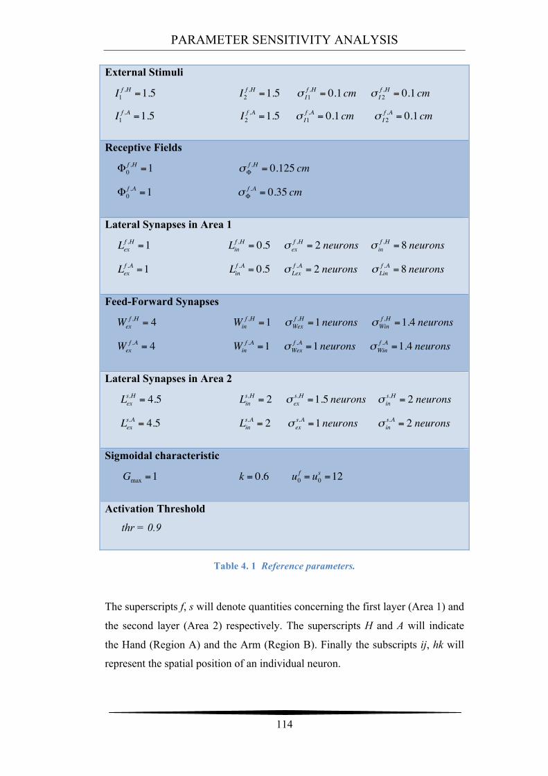
PARAMETER SENSITIVITY ANALYSIS
114
External Stimuli
I1f ,H =1.5 I2
f ,H =1.5 ! I1f ,H = 0.1 cm ! I 2
f ,H = 0.1 cm
I1f ,A =1.5 I2
f ,A =1.5 ! I1f ,A = 0.1 cm ! I 2
f ,A = 0.1 cm
Receptive Fields
!0f ,H =1 !!
f ,H = 0.125 cm
!0f ,A =1 !!
f ,A = 0.35 cm
Lateral Synapses in Area 1
Lexf ,H =1 Lin
f ,H = 0.5 ! exf ,H = 2 neurons ! in
f ,H = 8 neurons
Lexf ,A =1 Lin
f ,A = 0.5 ! Lexf ,A = 2 neurons ! Lin
f ,A = 8 neurons
Feed-Forward Synapses
Wexf ,H = 4 Win
f ,H =1 !Wexf ,H =1neurons !Win
f ,H =1.4 neurons
Wexf ,A = 4 Win
f ,A =1 !Wexf ,A =1neurons !Win
f ,A =1.4 neurons
Lateral Synapses in Area 2
Lexs,H = 4.5 Lin
s,H = 2 ! exs,H =1.5 neurons ! in
s,H = 2 neurons
Lexs,A = 4.5 Lin
s,A = 2 ! exs,A =1neurons ! in
s,A = 2 neurons
Sigmoidal characteristic
Gmax =1 k = 0.6 u f0 = u
s0 =12
Activation Threshold thr = 0.9
Table 4. 1 Reference parameters.
The superscripts f, s will denote quantities concerning the first layer (Area 1) and
the second layer (Area 2) respectively. The superscripts H and A will indicate
the Hand (Region A) and the Arm (Region B). Finally the subscripts ij, hk will
represent the spatial position of an individual neuron.
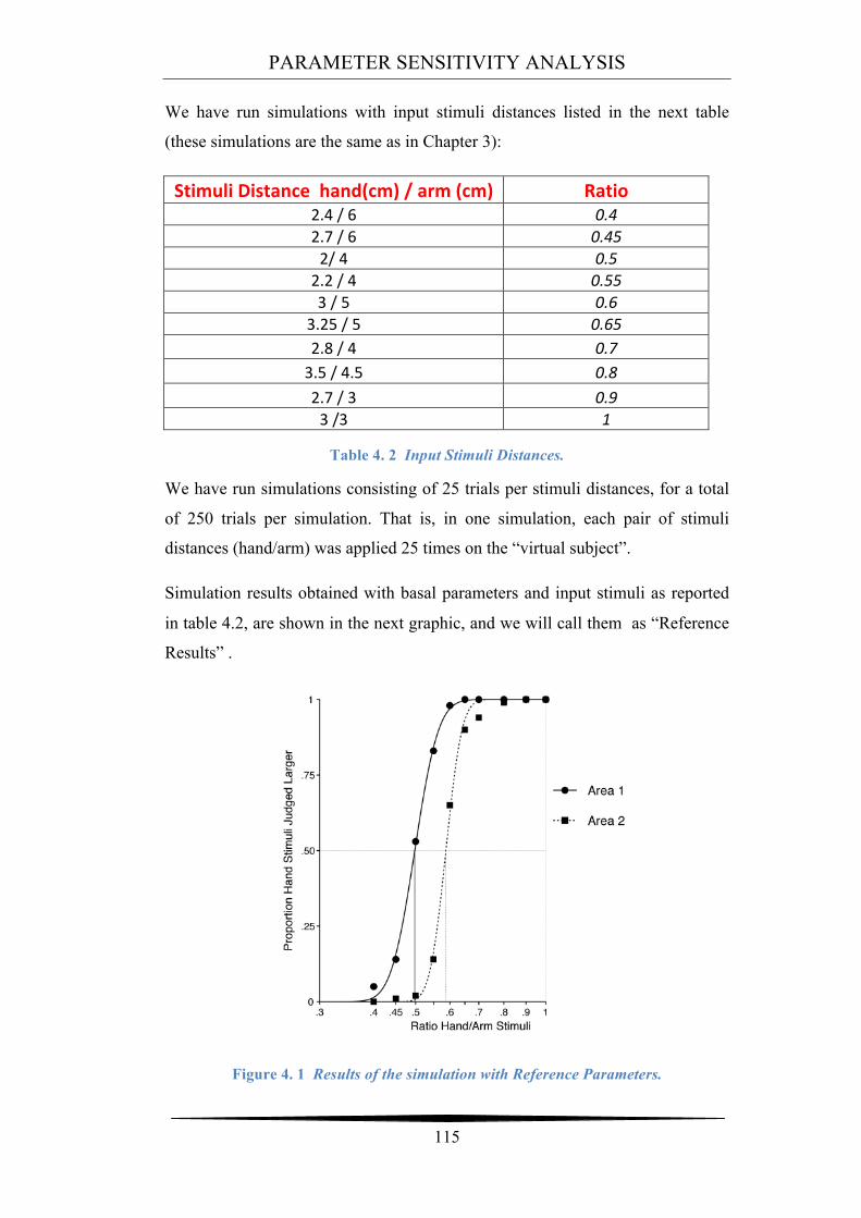
PARAMETER SENSITIVITY ANALYSIS
115
We have run simulations with input stimuli distances listed in the next table
(these simulations are the same as in Chapter 3):
Stimuli Distance hand(cm) / arm (cm) Ratio 2.4 / 6 0.4 2.7 / 6 0.45 2/ 4 0.5 2.2 / 4 0.55 3 / 5 0.6
3.25 / 5 0.65 2.8 / 4 0.7 3.5 / 4.5 0.8 2.7 / 3 0.9 3 /3 1
Table 4. 2 Input Stimuli Distances.
We have run simulations consisting of 25 trials per stimuli distances, for a total
of 250 trials per simulation. That is, in one simulation, each pair of stimuli
distances (hand/arm) was applied 25 times on the “virtual subject”.
Simulation results obtained with basal parameters and input stimuli as reported
in table 4.2, are shown in the next graphic, and we will call them as “Reference
Results” .
Figure 4. 1 Results of the simulation with Reference Parameters.
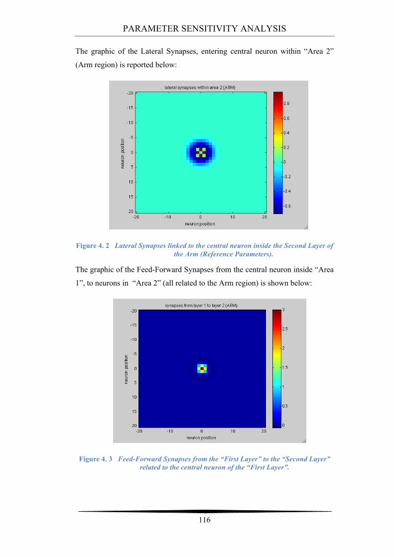
PARAMETER SENSITIVITY ANALYSIS
116
The graphic of the Lateral Synapses, entering central neuron within “Area 2”
(Arm region) is reported below:
Figure 4. 2 Lateral Synapses linked to the central neuron inside the Second Layer of the Arm (Reference Parameters).
The graphic of the Feed-Forward Synapses from the central neuron inside “Area
1”, to neurons in “Area 2” (all related to the Arm region) is shown below:
Figure 4. 3 Feed-Forward Synapses from the “First Layer” to the “Second Layer” related to the central neuron of the “First Layer”.

PARAMETER SENSITIVITY ANALYSIS
117
Remember that each little coloured square in position (i,j) represents the
intensity of the feed forward synapse that reaches the neuron inside Area 2 in
position (i,j).
Finally, the next table shows the entity of the Weber’s Illusion and the Rescaling
Process, still related to the “Reference Results”:
PSE Weber’s Illusion = 1 – PSE
Rescaling Process = PSE Area2 – PSE Area1
First Layer 0.5 0,5 0.09 Second Layer 0.59 0,41
Table 4. 3 Reference Results.
4.2 The Changed Parameters
In this study we have focused the attention on the neural network of the Arm,
changing parameters concerning feed forward-synapses and lateral synapses
within Area 2. Below, a list of the parameters that have been changed:
• !!"!,! (Lateral Synapses within Area 2: standard deviation of the
excitatory component)
• !!"!,! (Lateral Synapses within Area 2: standard deviation of the
inhibitory component)
• !!"!,! (Lateral Synapses within Area 2: intensity of the excitatory
component)
• !!"!,! (Lateral Synapses within Area 2: intensity of the inhibitory
component)
• !!"#!,! (Feed-Forward Synapses: standard deviation of the excitatory
component)
• !!"#!,! (Feed-Forward Synapses: standard deviation of the inhibitory
component)
• !!"!,! (Feed-Forward Synapses: intensity of the excitatory component)
• !!"!,! (Feed-Forward Synapses: intensity of the inhibitory component)
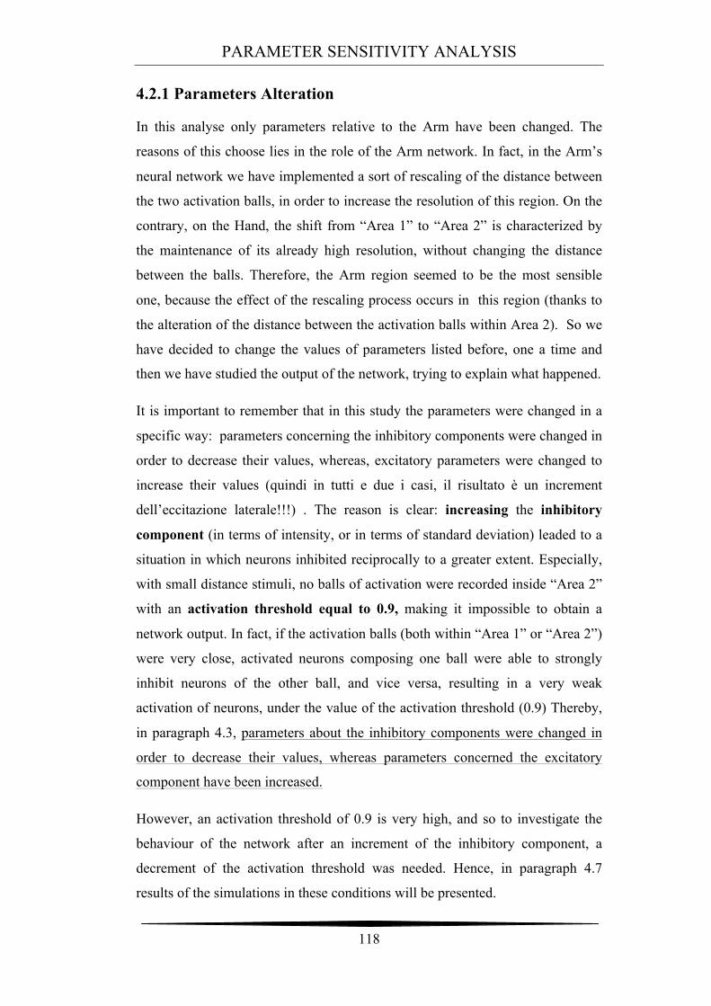
PARAMETER SENSITIVITY ANALYSIS
118
4.2.1 Parameters Alteration
In this analyse only parameters relative to the Arm have been changed. The
reasons of this choose lies in the role of the Arm network. In fact, in the Arm’s
neural network we have implemented a sort of rescaling of the distance between
the two activation balls, in order to increase the resolution of this region. On the
contrary, on the Hand, the shift from “Area 1” to “Area 2” is characterized by
the maintenance of its already high resolution, without changing the distance
between the balls. Therefore, the Arm region seemed to be the most sensible
one, because the effect of the rescaling process occurs in this region (thanks to
the alteration of the distance between the activation balls within Area 2). So we
have decided to change the values of parameters listed before, one a time and
then we have studied the output of the network, trying to explain what happened.
It is important to remember that in this study the parameters were changed in a
specific way: parameters concerning the inhibitory components were changed in
order to decrease their values, whereas, excitatory parameters were changed to
increase their values (quindi in tutti e due i casi, il risultato è un increment
dell’eccitazione laterale!!!) . The reason is clear: increasing the inhibitory
component (in terms of intensity, or in terms of standard deviation) leaded to a
situation in which neurons inhibited reciprocally to a greater extent. Especially,
with small distance stimuli, no balls of activation were recorded inside “Area 2”
with an activation threshold equal to 0.9, making it impossible to obtain a
network output. In fact, if the activation balls (both within “Area 1” or “Area 2”)
were very close, activated neurons composing one ball were able to strongly
inhibit neurons of the other ball, and vice versa, resulting in a very weak
activation of neurons, under the value of the activation threshold (0.9) Thereby,
in paragraph 4.3, parameters about the inhibitory components were changed in
order to decrease their values, whereas parameters concerned the excitatory
component have been increased.
However, an activation threshold of 0.9 is very high, and so to investigate the
behaviour of the network after an increment of the inhibitory component, a
decrement of the activation threshold was needed. Hence, in paragraph 4.7
results of the simulations in these conditions will be presented.
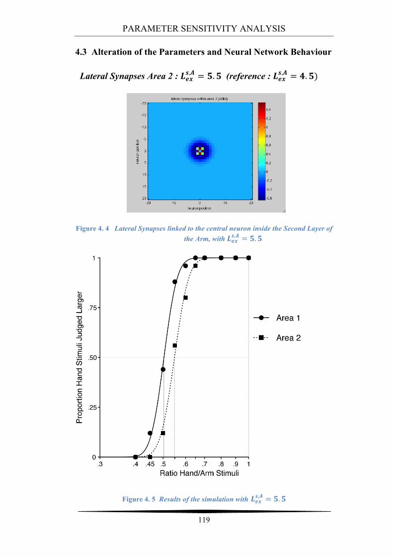
PARAMETER SENSITIVITY ANALYSIS
119
4.3 Alteration of the Parameters and Neural Network Behaviour
Lateral Synapses Area 2 : !!"!,! = !.! (reference : !!"
!,! = !.!)
Figure 4. 4 Lateral Synapses linked to the central neuron inside the Second Layer of the Arm, with !!"
!,! = !.!
Figure 4. 5 Results of the simulation with !!"!,! = !.!
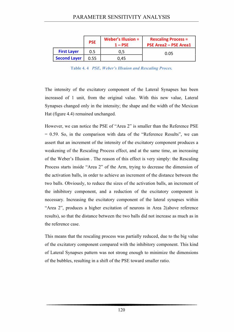
PARAMETER SENSITIVITY ANALYSIS
120
PSE Weber’s Illusion = 1 – PSE
Rescaling Process = PSE Area2 – PSE Area1
First Layer 0.5 0,5 0.05 Second Layer 0.55 0,45
Table 4. 4 PSE, Weber’s Illsuion and Rescaling Proces.
The intensity of the excitatory component of the Lateral Synapses has been
increased of 1 unit, from the original value. With this new value, Lateral
Synapses changed only in the intensity; the shape and the width of the Mexican
Hat (figure 4.4) remained unchanged.
However, we can notice the PSE of “Area 2” is smaller than the Reference PSE
= 0.59. So, in the comparison with data of the “Reference Results”, we can
assert that an increment of the intensity of the excitatory component produces a
weakening of the Rescaling Process effect, and at the same time, an increasing
of the Weber’s Illusion . The reason of this effect is very simply: the Rescaling
Process starts inside “Area 2” of the Arm, trying to decrease the dimension of
the activation balls, in order to achieve an increment of the distance between the
two balls. Obviously, to reduce the sizes of the activation balls, an increment of
the inhibitory component, and a reduction of the excitatory component is
necessary. Increasing the excitatory component of the lateral synapses within
“Area 2”, produces a higher excitation of neurons in Area 2(above reference
results), so that the distance between the two balls did not increase as much as in
the reference case.
This means that the rescaling process was partially reduced, due to the big value
of the excitatory component compared with the inhibitory component. This kind
of Lateral Synapses pattern was not strong enough to minimize the dimensions
of the bubbles, resulting in a shift of the PSE toward smaller ratio.
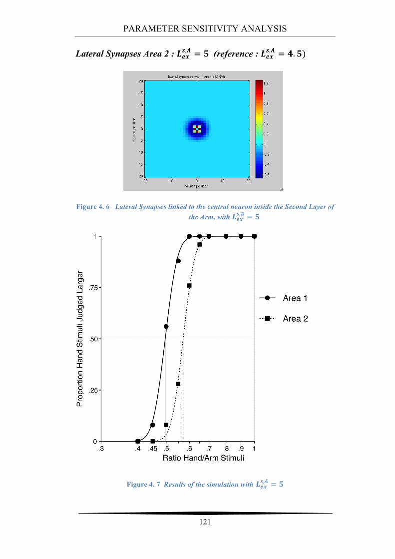
PARAMETER SENSITIVITY ANALYSIS
121
Lateral Synapses Area 2 : !!"!,! = ! (reference : !!"
!,! = !.!)
Figure 4. 6 Lateral Synapses linked to the central neuron inside the Second Layer of the Arm, with !!"
!,! = !
Figure 4. 7 Results of the simulation with !!"!,! = !
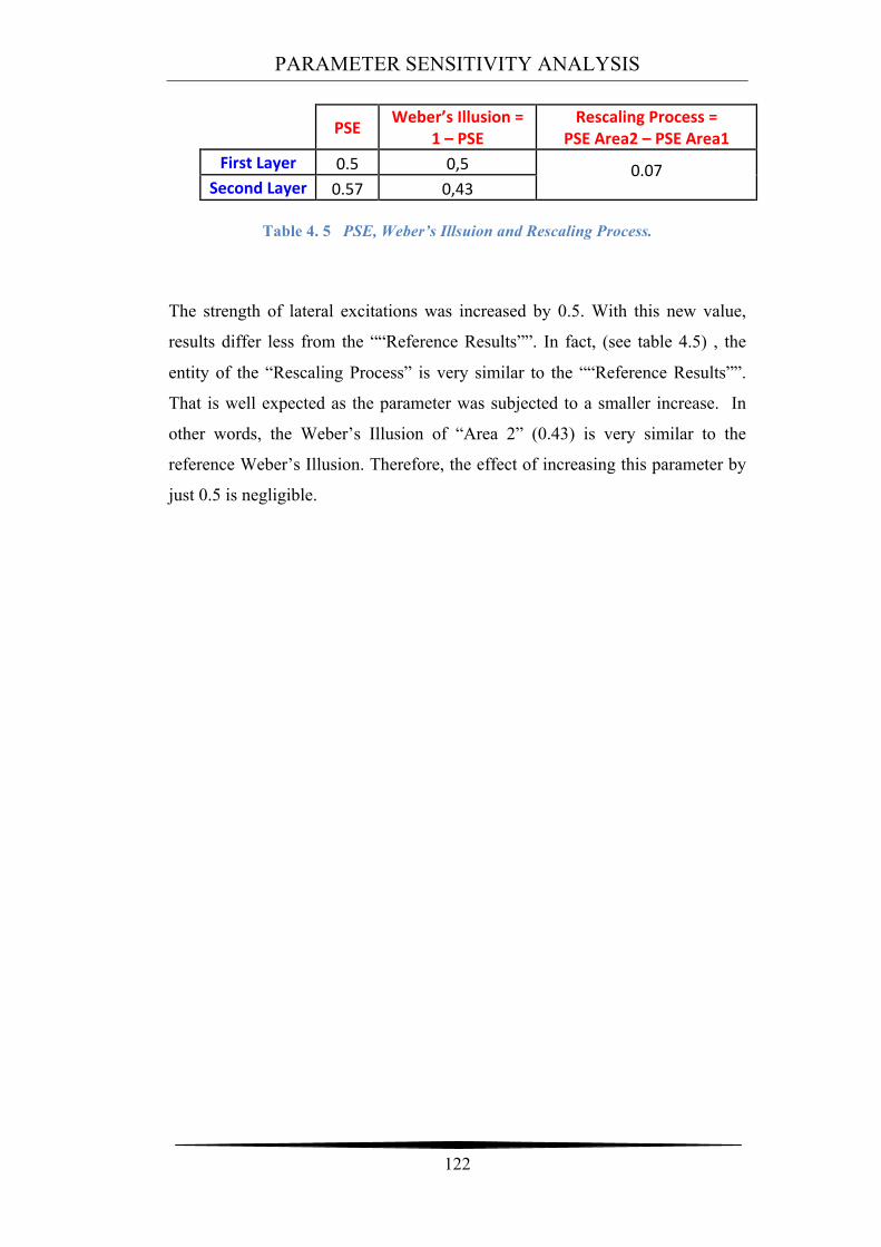
PARAMETER SENSITIVITY ANALYSIS
122
PSE Weber’s Illusion = 1 – PSE
Rescaling Process = PSE Area2 – PSE Area1
First Layer 0.5 0,5 0.07 Second Layer 0.57 0,43
Table 4. 5 PSE, Weber’s Illsuion and Rescaling Process.
The strength of lateral excitations was increased by 0.5. With this new value,
results differ less from the ““Reference Results””. In fact, (see table 4.5) , the
entity of the “Rescaling Process” is very similar to the ““Reference Results””.
That is well expected as the parameter was subjected to a smaller increase. In
other words, the Weber’s Illusion of “Area 2” (0.43) is very similar to the
reference Weber’s Illusion. Therefore, the effect of increasing this parameter by
just 0.5 is negligible.
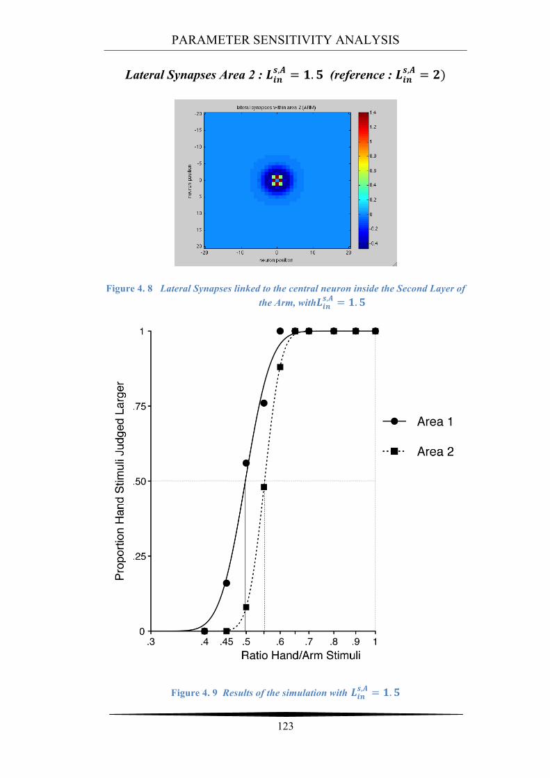
PARAMETER SENSITIVITY ANALYSIS
123
Lateral Synapses Area 2 : !!"!,! = !.! (reference : !!"
!,! = !)
Figure 4. 8 Lateral Synapses linked to the central neuron inside the Second Layer of the Arm, with!!"
!,! = !.!
Figure 4. 9 Results of the simulation with !!"!,! = !.!
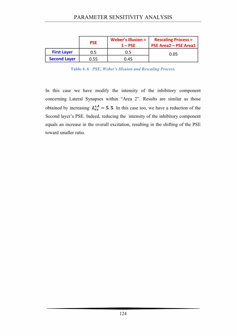
PARAMETER SENSITIVITY ANALYSIS
124
PSE Weber’s Illusion = 1 – PSE
Rescaling Process = PSE Area2 – PSE Area1
First Layer 0.5 0.5 0.05 Second Layer 0.55 0.45
Table 4. 6 PSE, Weber’s Illsuion and Rescaling Process.
In this case we have modify the intensity of the inhibitory component
concerning Lateral Synapses within “Area 2”. Results are similar as those
obtained by increasing !!"!,! = !.!. In this case too, we have a reduction of the
Second layer’s PSE. Indeed, reducing the intensity of the inhibitory component
equals an increase in the overall excitation, resulting in the shifting of the PSE
toward smaller ratio.
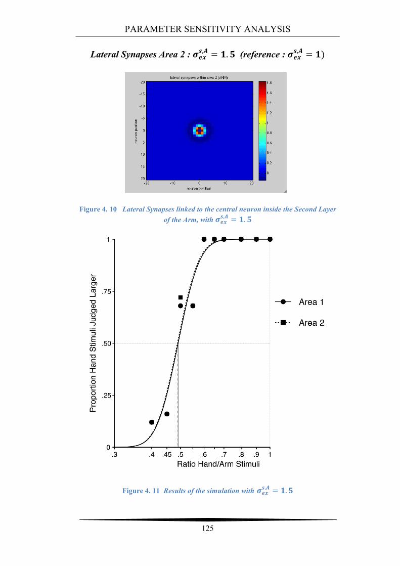
PARAMETER SENSITIVITY ANALYSIS
125
Lateral Synapses Area 2 : !!"!,! = !.! (reference : !!"
!,! = !)
Figure 4. 10 Lateral Synapses linked to the central neuron inside the Second Layer of the Arm, with !!"
!,! = !.!
Figure 4. 11 Results of the simulation with !!"!,! = !.!
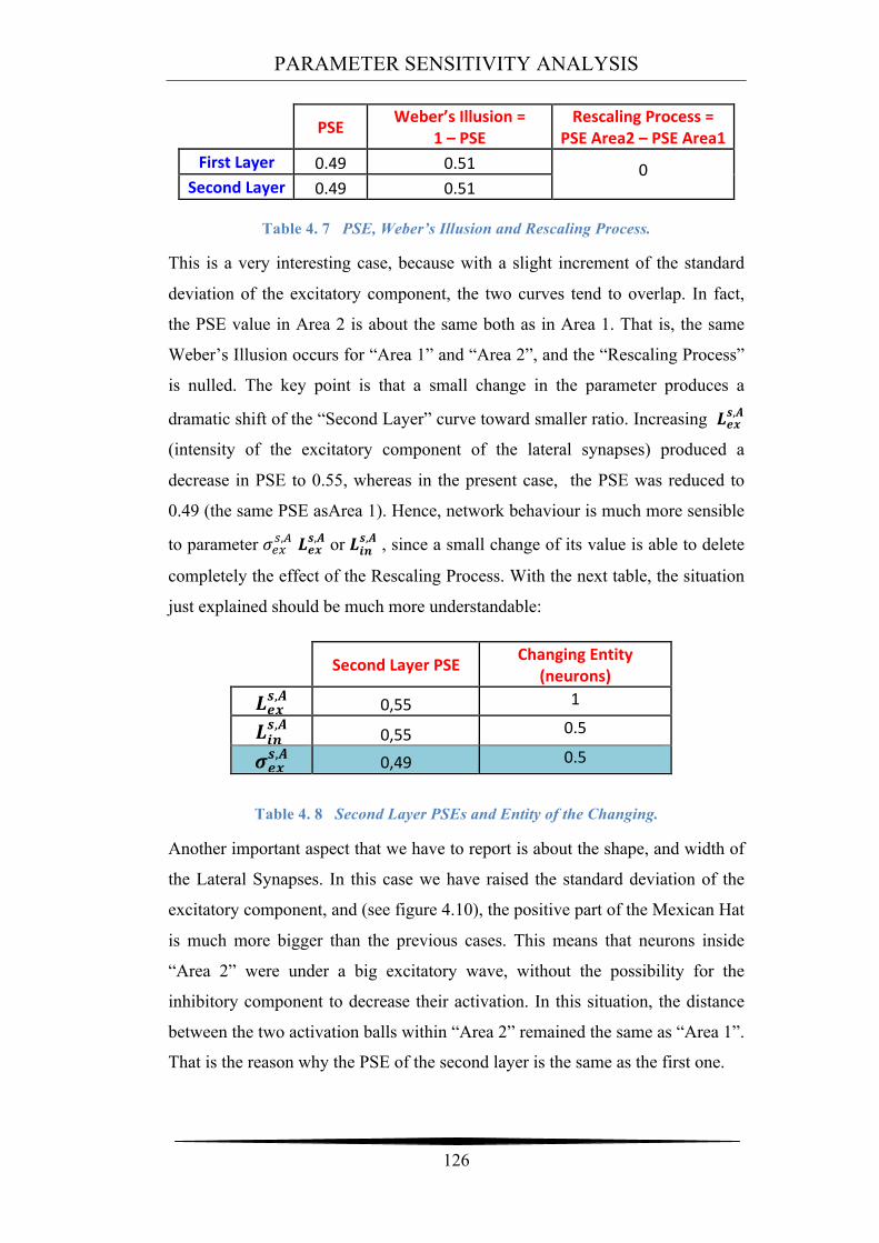
PARAMETER SENSITIVITY ANALYSIS
126
PSE Weber’s Illusion = 1 – PSE
Rescaling Process = PSE Area2 – PSE Area1
First Layer 0.49 0.51 0 Second Layer 0.49 0.51
Table 4. 7 PSE, Weber’s Illusion and Rescaling Process.
This is a very interesting case, because with a slight increment of the standard
deviation of the excitatory component, the two curves tend to overlap. In fact,
the PSE value in Area 2 is about the same both as in Area 1. That is, the same
Weber’s Illusion occurs for “Area 1” and “Area 2”, and the “Rescaling Process”
is nulled. The key point is that a small change in the parameter produces a
dramatic shift of the “Second Layer” curve toward smaller ratio. Increasing !!"!,!
(intensity of the excitatory component of the lateral synapses) produced a
decrease in PSE to 0.55, whereas in the present case, the PSE was reduced to
0.49 (the same PSE asArea 1). Hence, network behaviour is much more sensible
to parameter !!"!,! !!"!,! or !!"
!,! , since a small change of its value is able to delete
completely the effect of the Rescaling Process. With the next table, the situation
just explained should be much more understandable:
Second Layer PSE Changing Entity (neurons)
!!"!,! 0,55 1
!!"!,! 0,55 0.5
!!"!,! 0,49 0.5
Table 4. 8 Second Layer PSEs and Entity of the Changing.
Another important aspect that we have to report is about the shape, and width of
the Lateral Synapses. In this case we have raised the standard deviation of the
excitatory component, and (see figure 4.10), the positive part of the Mexican Hat
is much more bigger than the previous cases. This means that neurons inside
“Area 2” were under a big excitatory wave, without the possibility for the
inhibitory component to decrease their activation. In this situation, the distance
between the two activation balls within “Area 2” remained the same as “Area 1”.
That is the reason why the PSE of the second layer is the same as the first one.
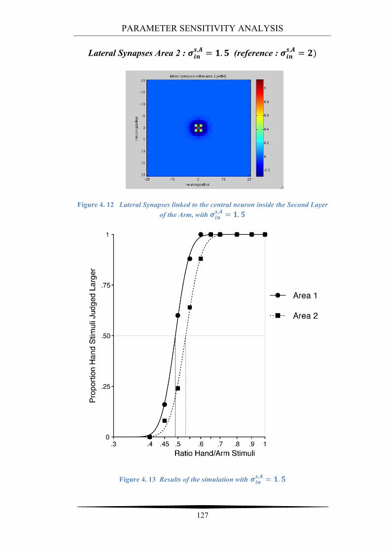
PARAMETER SENSITIVITY ANALYSIS
127
Lateral Synapses Area 2 : !!"!,! = !.! (reference : !!"
!,! = !)
Figure 4. 12 Lateral Synapses linked to the central neuron inside the Second Layer of the Arm, with !!"
!,! = !.!
Figure 4. 13 Results of the simulation with !!"!,! = !.!
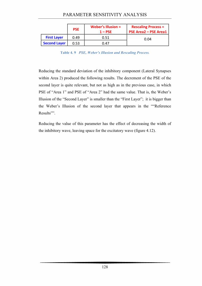
PARAMETER SENSITIVITY ANALYSIS
128
PSE Weber’s Illusion = 1 – PSE
Rescaling Process = PSE Area2 – PSE Area1
First Layer 0.49 0.51 0.04 Second Layer 0.53 0.47
Table 4. 9 PSE, Weber’s Illusion and Rescaling Process.
Reducing the standard deviation of the inhibitory component (Lateral Synapses
within Area 2) produced the following results. The decrement of the PSE of the
second layer is quite relevant, but not as high as in the previous case, in which
PSE of “Area 1” and PSE of “Area 2” had the same value. That is, the Weber’s
Illusion of the “Second Layer” is smaller than the “First Layer”; it is bigger than
the Weber’s Illusion of the second layer that appears in the ““Reference
Results””.
Reducing the value of this parameter has the effect of decreasing the width of
the inhibitory wave, leaving space for the excitatory wave (figure 4.12).
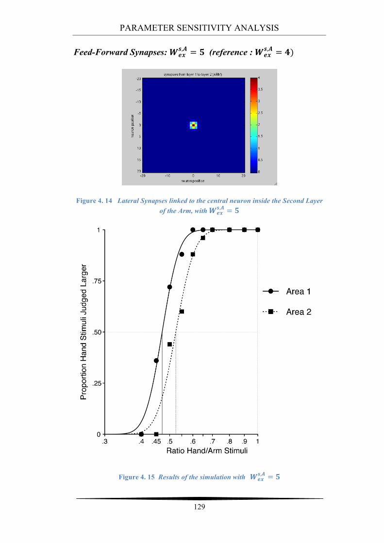
PARAMETER SENSITIVITY ANALYSIS
129
Feed-Forward Synapses: !!"!,! = ! (reference : !!"
!,! = !)
Figure 4. 14 Lateral Synapses linked to the central neuron inside the Second Layer of the Arm, with !!"
!,! = !
Figure 4. 15 Results of the simulation with !!"!,! = !
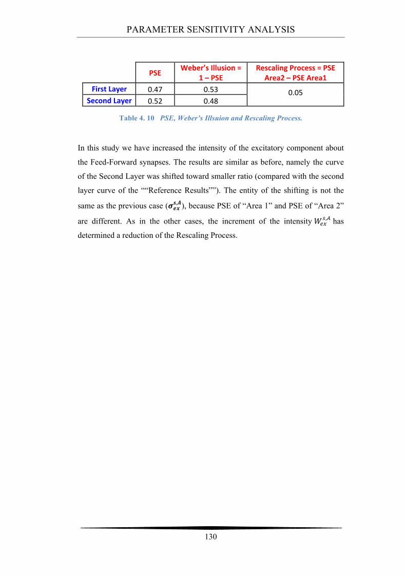
PARAMETER SENSITIVITY ANALYSIS
130
PSE Weber’s Illusion = 1 – PSE
Rescaling Process = PSE Area2 – PSE Area1
First Layer 0.47 0.53 0.05 Second Layer 0.52 0.48
Table 4. 10 PSE, Weber’s Illsuion and Rescaling Process.
In this study we have increased the intensity of the excitatory component about
the Feed-Forward synapses. The results are similar as before, namely the curve
of the Second Layer was shifted toward smaller ratio (compared with the second
layer curve of the ““Reference Results””). The entity of the shifting is not the
same as the previous case (!!"!,!), because PSE of “Area 1” and PSE of “Area 2”
are different. As in the other cases, the increment of the intensity !!"!,! has
determined a reduction of the Rescaling Process.
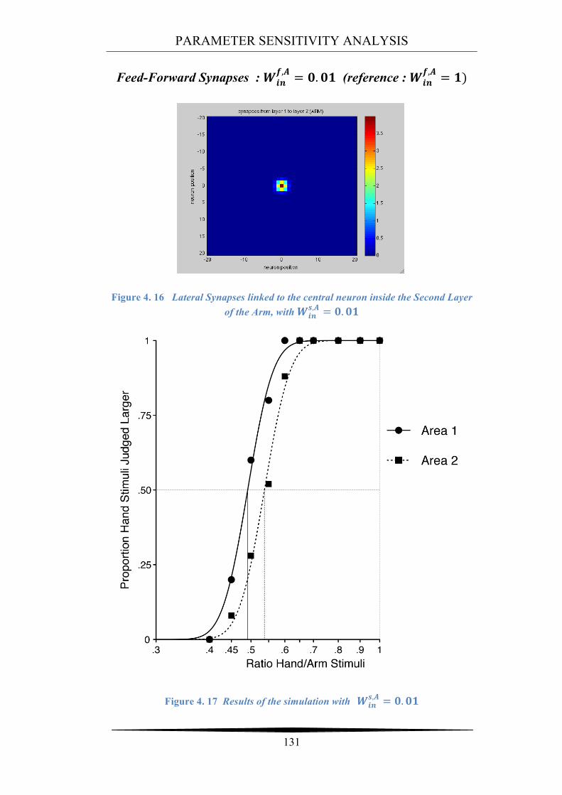
PARAMETER SENSITIVITY ANALYSIS
131
Feed-Forward Synapses : !!"!,! = !.!" (reference : !!"
!,! = !)
Figure 4. 16 Lateral Synapses linked to the central neuron inside the Second Layer of the Arm, with !!"
!,! = !.!"
Figure 4. 17 Results of the simulation with !!"!,! = !.!"
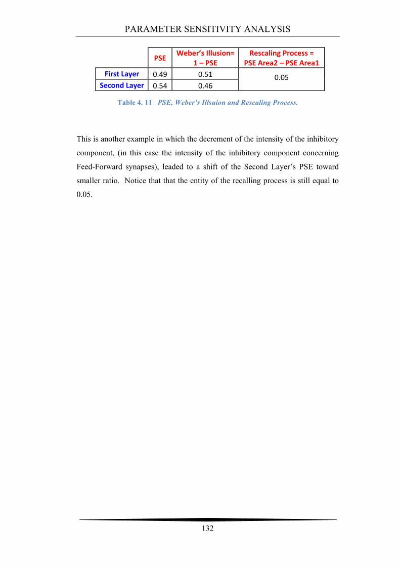
PARAMETER SENSITIVITY ANALYSIS
132
PSE Weber’s Illusion= 1 – PSE
Rescaling Process = PSE Area2 – PSE Area1
First Layer 0.49 0.51 0.05 Second Layer 0.54 0.46
Table 4. 11 PSE, Weber’s Illsuion and Rescaling Process.
This is another example in which the decrement of the intensity of the inhibitory
component, (in this case the intensity of the inhibitory component concerning
Feed-Forward synapses), leaded to a shift of the Second Layer’s PSE toward
smaller ratio. Notice that that the entity of the recalling process is still equal to
0.05.
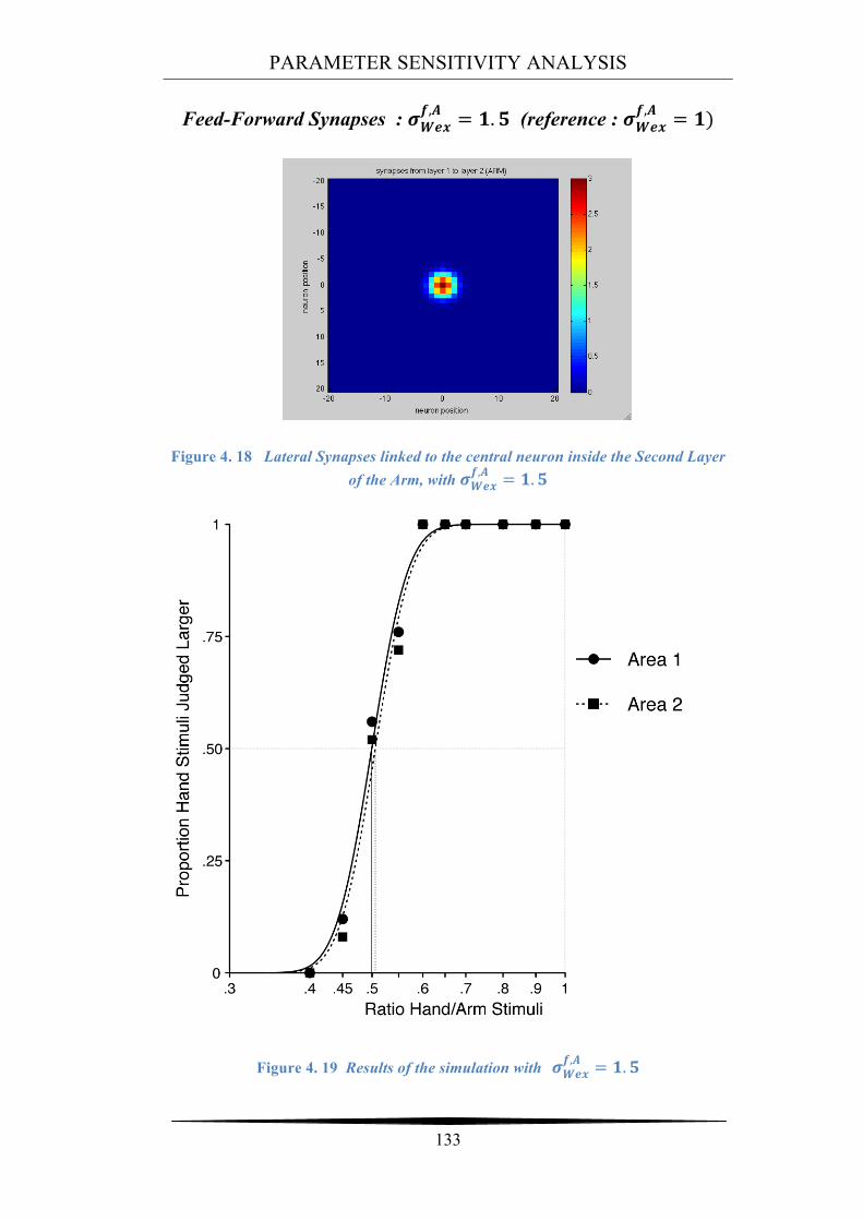
PARAMETER SENSITIVITY ANALYSIS
133
Feed-Forward Synapses : !!"#!,! = !.! (reference : !!"#
!,! = !)
Figure 4. 18 Lateral Synapses linked to the central neuron inside the Second Layer of the Arm, with !!"#
!,! = !.!
Figure 4. 19 Results of the simulation with !!"#!,! = !.!
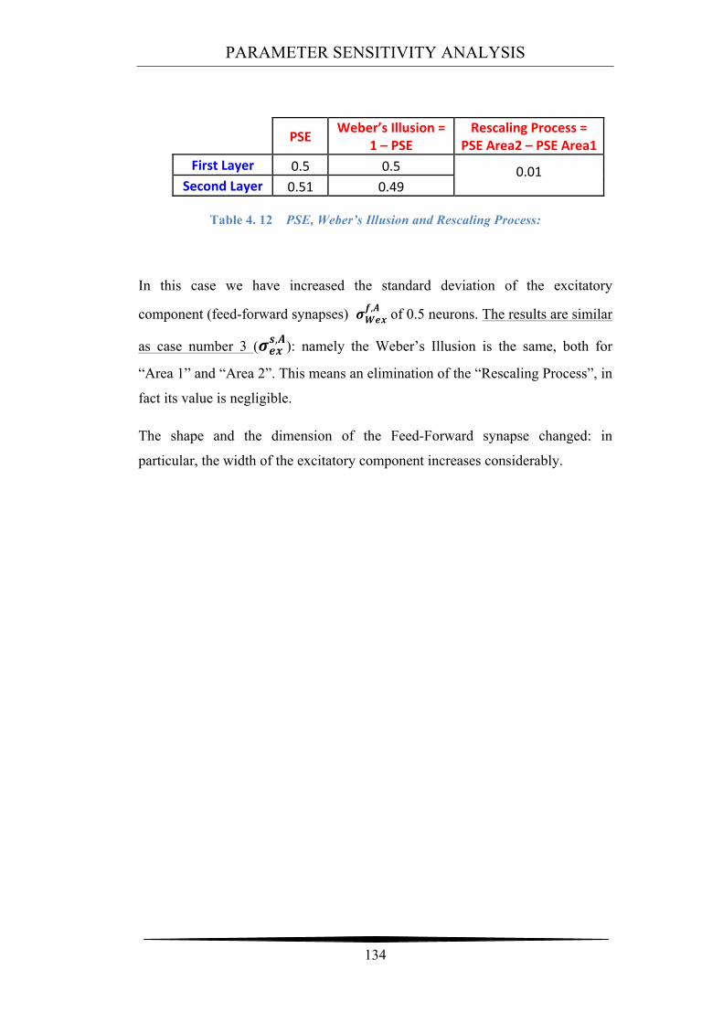
PARAMETER SENSITIVITY ANALYSIS
134
PSE Weber’s Illusion = 1 – PSE
Rescaling Process = PSE Area2 – PSE Area1
First Layer 0.5 0.5 0.01 Second Layer 0.51 0.49
Table 4. 12 PSE, Weber’s Illusion and Rescaling Process:
In this case we have increased the standard deviation of the excitatory
component (feed-forward synapses) !!"#!,! of 0.5 neurons. The results are similar
as case number 3 (!!"!,!): namely the Weber’s Illusion is the same, both for
“Area 1” and “Area 2”. This means an elimination of the “Rescaling Process”, in
fact its value is negligible.
The shape and the dimension of the Feed-Forward synapse changed: in
particular, the width of the excitatory component increases considerably.
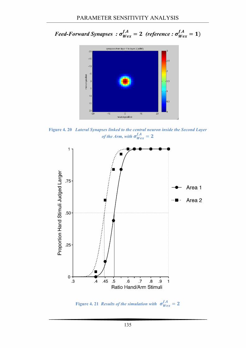
PARAMETER SENSITIVITY ANALYSIS
135
Feed-Forward Synapses : !!"#!,! = ! (reference : !!"#
!,! = !)
Figure 4. 20 Lateral Synapses linked to the central neuron inside the Second Layer of the Arm, with !!"#
!,! = !
Figure 4. 21 Results of the simulation with !!"#!,! = !
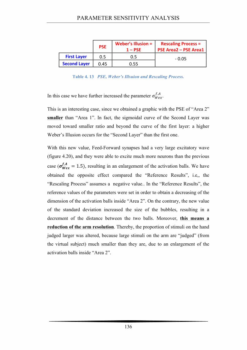
PARAMETER SENSITIVITY ANALYSIS
136
PSE Weber’s Illusion = 1 – PSE
Rescaling Process = PSE Area2 – PSE Area1
First Layer 0.5 0.5 -‐ 0.05 Second Layer 0.45 0.55
Table 4. 13 PSE, Weber’s Illsuion and Rescaling Process.
In this case we have further increased the parameter !!"#!,! .
This is an interesting case, since we obtained a graphic with the PSE of “Area 2”
smaller than “Area 1”. In fact, the sigmoidal curve of the Second Layer was
moved toward smaller ratio and beyond the curve of the first layer: a higher
Weber’s Illusion occurs for the “Second Layer” than the first one.
With this new value, Feed-Forward synapses had a very large excitatory wave
(figure 4.20), and they were able to excite much more neurons than the previous
case (!!"#!,! = 1.5), resulting in an enlargement of the activation balls. We have
obtained the opposite effect compared the “Reference Results”, i.e,, the
“Rescaling Process” assumes a negative value.. In the “Reference Results”, the
reference values of the parameters were set in order to obtain a decreasing of the
dimension of the activation balls inside “Area 2”. On the contrary, the new value
of the standard deviation increased the size of the bubbles, resulting in a
decrement of the distance between the two balls. Moreover, this means a
reduction of the arm resolution. Thereby, the proportion of stimuli on the hand
judged larger was altered, because large stimuli on the arm are “judged” (from
the virtual subject) much smaller than they are, due to an enlargement of the
activation balls inside “Area 2”.
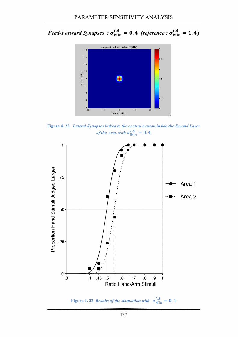
PARAMETER SENSITIVITY ANALYSIS
137
Feed-Forward Synapses : !!"#!,! = !.! (reference : !!"#
!,! = !.!)
Figure 4. 22 Lateral Synapses linked to the central neuron inside the Second Layer of the Arm, with !!"#
!,! = !.!
Figure 4. 23 Results of the simulation with !!"#!,! = !.!
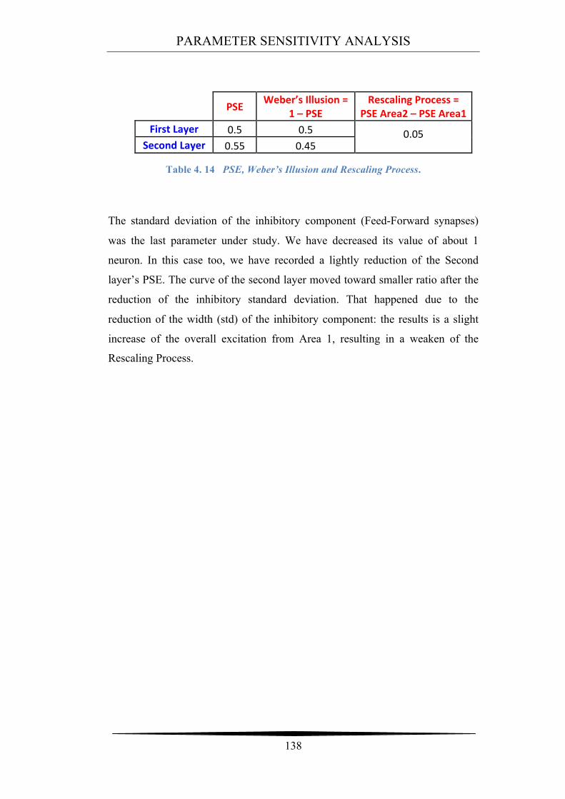
PARAMETER SENSITIVITY ANALYSIS
138
PSE Weber’s Illusion = 1 – PSE
Rescaling Process = PSE Area2 – PSE Area1
First Layer 0.5 0.5 0.05 Second Layer 0.55 0.45
Table 4. 14 PSE, Weber’s Illusion and Rescaling Process.
The standard deviation of the inhibitory component (Feed-Forward synapses)
was the last parameter under study. We have decreased its value of about 1
neuron. In this case too, we have recorded a lightly reduction of the Second
layer’s PSE. The curve of the second layer moved toward smaller ratio after the
reduction of the inhibitory standard deviation. That happened due to the
reduction of the width (std) of the inhibitory component: the results is a slight
increase of the overall excitation from Area 1, resulting in a weaken of the
Rescaling Process.
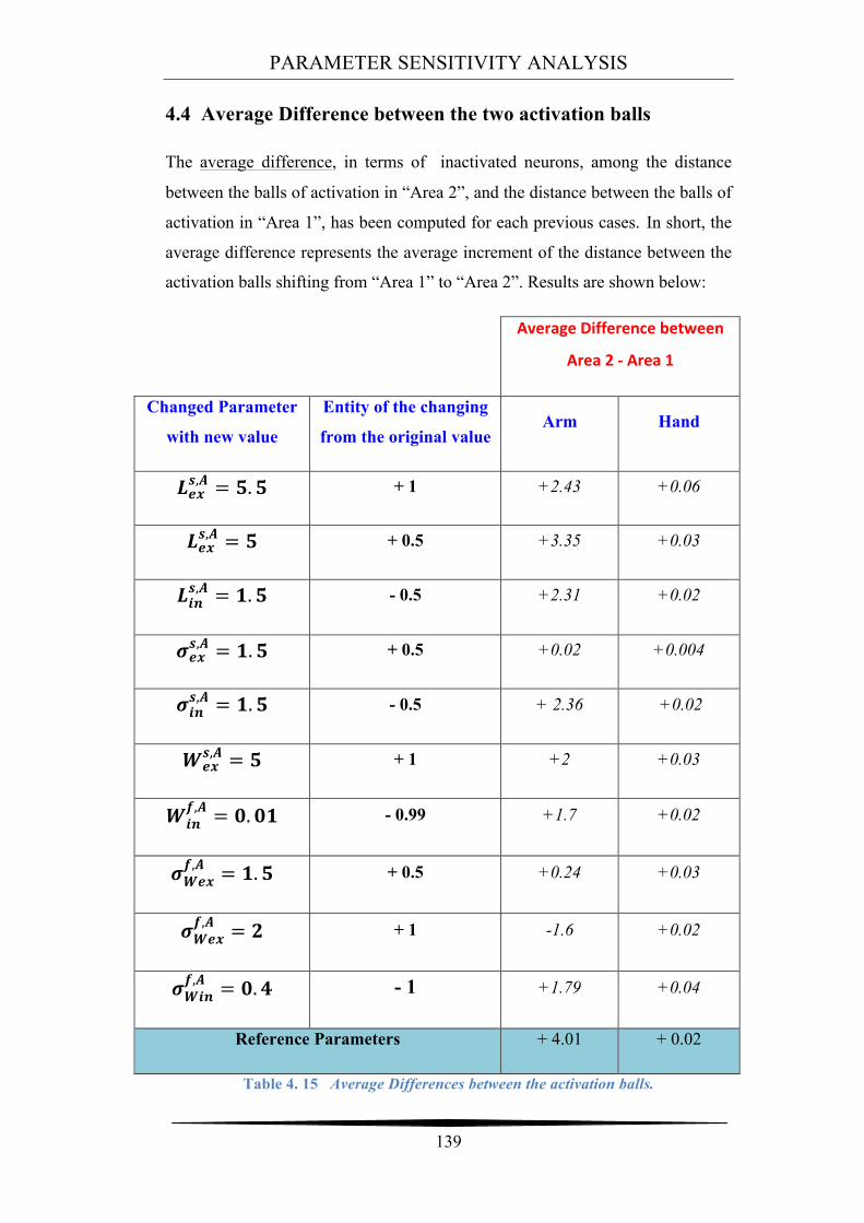
PARAMETER SENSITIVITY ANALYSIS
139
4.4 Average Difference between the two activation balls
The average difference, in terms of inactivated neurons, among the distance
between the balls of activation in “Area 2”, and the distance between the balls of
activation in “Area 1”, has been computed for each previous cases. In short, the
average difference represents the average increment of the distance between the
activation balls shifting from “Area 1” to “Area 2”. Results are shown below:
Average Difference between
Area 2 -‐ Area 1
Changed Parameter
with new value
Entity of the changing
from the original value Arm Hand
!!"!,! = !.! + 1 +2.43 +0.06
!!"!,! = ! + 0.5 +3.35 +0.03
!!"!,! = !.! - 0.5 +2.31 +0.02
!!"!,! = !.! + 0.5 +0.02 +0.004
!!"!,! = !.! - 0.5 + 2.36 +0.02
!!"!,! = ! + 1 +2 +0.03
!!"!,! = !.!" - 0.99 +1.7 +0.02
!!"#!,! = !.! + 0.5 +0.24 +0.03
!!"#!,! = ! + 1 -1.6 +0.02
!!"#!,! = !.! - 1 +1.79 +0.04
Reference Parameters + 4.01 + 0.02
Table 4. 15 Average Differences between the activation balls.
PARAMETER SENSITIVITY ANALYSIS
140
The results highlighted in blue concern the simulation with reference
parameters:
In this kind of analyse we have modified only parameters concerning the Arm
region, so the Hand region was not affected by this changing: we can notice that
the average difference of the Hand is always equal zero in each case, just
because its parameters were kept constant in each case.
Positive signs denoted an increment of the distance between the activation balls
within “Area 2”, whereas, negative signs denoted a decrement of the distance
between the activation balls within “Area 2”.
The first consideration was about the comparison among the value of the
average difference obtained with “Reference Parameter” (table 4.1), and the
average difference obtained by changing of one parameter per time. Obviously,
in the Arm’s case, the average difference changes every time. However, the
average difference of the Arm is always abundantly under the value recorded in
the Reference Situation (+ 4.01). Hence, the increment of the resolution on the
Arm was reduced, or completely absent (see cases in which the average
difference is equal 0), when changing one parameter; indeed, the distance
between the activation balls in “Area 2” is always under 2.5 neurons. This value
might be not sufficient to implement a proper Rescaling Process.
Cases !!"!,! = !.! and !!"#
!,! = !.! are the most interesting cases, because the
average difference is very close to zero, both for the Hand and Arm; hence, the
distance between the activation balls is the same both for “Area 1” and “Area
2”. Figure 4.11 And Figure 4.19 show that in these cases the two sigmoidal
curves are superimposed.
However with !!"#!,! = ! the average value decrease until -1.6: this means that
the two activation balls within “Area 2” have increased their size, and the
distance between them has been reduced of about 1.6 neurons. So, this is the
worst case in absolute, because with this value we have achieved a decrement in
the resolution of the Arm, namely a total opposite effect against the target of the
neural network.
PARAMETER SENSITIVITY ANALYSIS
141
4.5 Conclusion about the Sensitivity Analysis
Concerning the sensitivity analysis, we can conclude that the most sensible
parameters seemed to be the standard deviation of the excitatory component,
that appears in the Lateral Synapses (!!"!,!), and the standard deviation of the
excitatory component, defining Feed-Forward synapses (!!"#!,! ). Indeed (see
table 4.15, figure 4.11 and figure 4.19), alteration of these parameters produced a
dramatically change of the network, that affects the position of the PSE of the
second layer. Remember that the entity of the increase for these two standard
deviations was equal to 0.5. The same increase applied to the other parameters
still produced a shifting of the second layer curve toward smaller ratio, but the
entity of the shifting was much smaller compared with cases !!"!,! and !!"#
!,! .
Thereby, the network is extremely sensible to these parameters, since as light
alteration of their value null the “Rescaling Process”: in others words, the
Weber’s Illusion associated with “Area 2” remained the same as “Area 1”.
PARAMETER SENSITIVITY ANALYSIS
142
4.6 Sensitivity Analysis about the Activation Threshold
In addition to the sensitivity analysis conducted on the network parameters (in
particular, synapses parameters), we have investigated the behaviour of the
neural network after the alteration of a fundamental parameter: the activation
threshold for computation of perceived distance among two punctual stimuli.
This threshold separates between active and inactive neurons, and is
fundamental in the computation of the perceived distance as only inactivated
neurons participate in establishing the perceived distance. Until now, we have
hypothesized an activation threshold equal to 0.9. But, how do network output
change when this value is changed?
Activation balls mentioned in this thesis are groups of neurons in which every
neuron has a state of activation equal, or greater than the activation threshold.
Obviously, changing of the activation threshold affects the dimension of the
activation balls, because with a low threshold, the number of neurons considered
active increase (increasing the dimension of the ball). Vice versa, if the threshold
is high, balls will appear of smaller dimension.
In this paragraph I will show the output of the neural network for different
values of the activation threshold:
• Activation threshold = 0.8
• Activation threshold = 0.7
• Activation threshold = 0.5
• Activation threshold = 0.3
• Activation threshold = 0.1

PARAMETER SENSITIVITY ANALYSIS
143
Activation Threshold: !"# = !.! (reference : !"# = !.!)
Figure 4. 24 Results of the simulation with !"# = !.!
PSE Weber’s Illusion = 1 – PSE
Rescaling Process = PSE Area2 – PSE Area1
First Layer 0.5 0.5 0.07 Second Layer 0.57 0.43
Table 4. 16 PSE, Weber’s Illsuion and Rescaling Process.

PARAMETER SENSITIVITY ANALYSIS
144
Activation Threshold: !"# = !.! (reference: !"# = !.!)
Figure 4. 25 Results of the simulation with !"# = !.!
PSE Weber’s Illusion = 1 – PSE
Rescaling Process = PSE Area2 – PSE Area1
First Layer 0.5 0.5 0.06 Second Layer 0.56 0.44
Table 4. 17 PSE, Weber’s Illsuion and Rescaling Process.
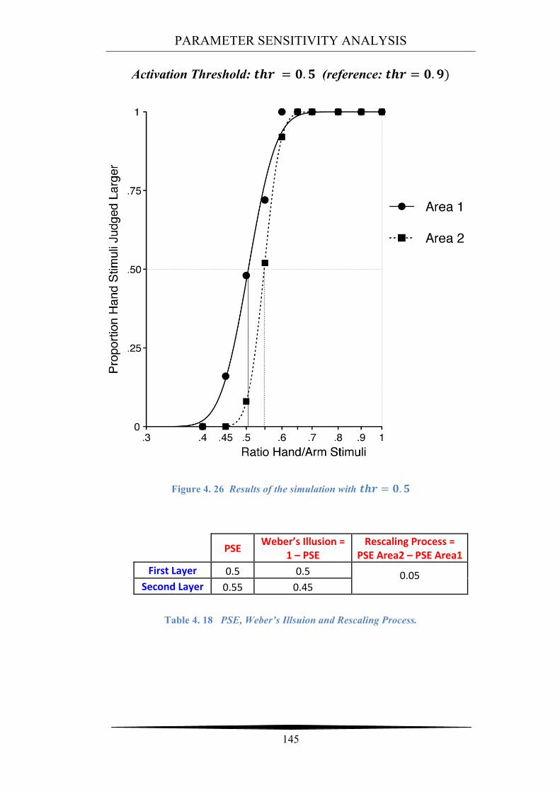
PARAMETER SENSITIVITY ANALYSIS
145
Activation Threshold: !"# = !.! (reference: !"# = !.!)
Figure 4. 26 Results of the simulation with !"# = !.!
PSE Weber’s Illusion = 1 – PSE
Rescaling Process = PSE Area2 – PSE Area1
First Layer 0.5 0.5 0.05 Second Layer 0.55 0.45
Table 4. 18 PSE, Weber’s Illsuion and Rescaling Process.
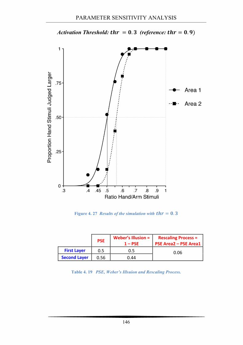
PARAMETER SENSITIVITY ANALYSIS
146
Activation Threshold: !"# = !.! (reference: !"# = !.!)
Figure 4. 27 Results of the simulation with !"# = !.!
PSE Weber’s Illusion = 1 – PSE
Rescaling Process = PSE Area2 – PSE Area1
First Layer 0.5 0.5 0.06 Second Layer 0.56 0.44
Table 4. 19 PSE, Weber’s Illsuion and Rescaling Process.
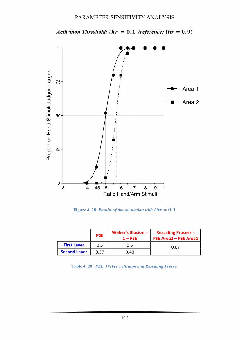
PARAMETER SENSITIVITY ANALYSIS
147
Activation Threshold: !"# = !.! (reference: !"# = !.!)
Figure 4. 28 Results of the simulation with !"# = !.!
PSE Weber’s Illusion = 1 – PSE
Rescaling Process = PSE Area2 – PSE Area1
First Layer 0.5 0.5 0.07 Second Layer 0.57 0.43
Table 4. 20 PSE, Weber’s Illsuion and Rescaling Proces.
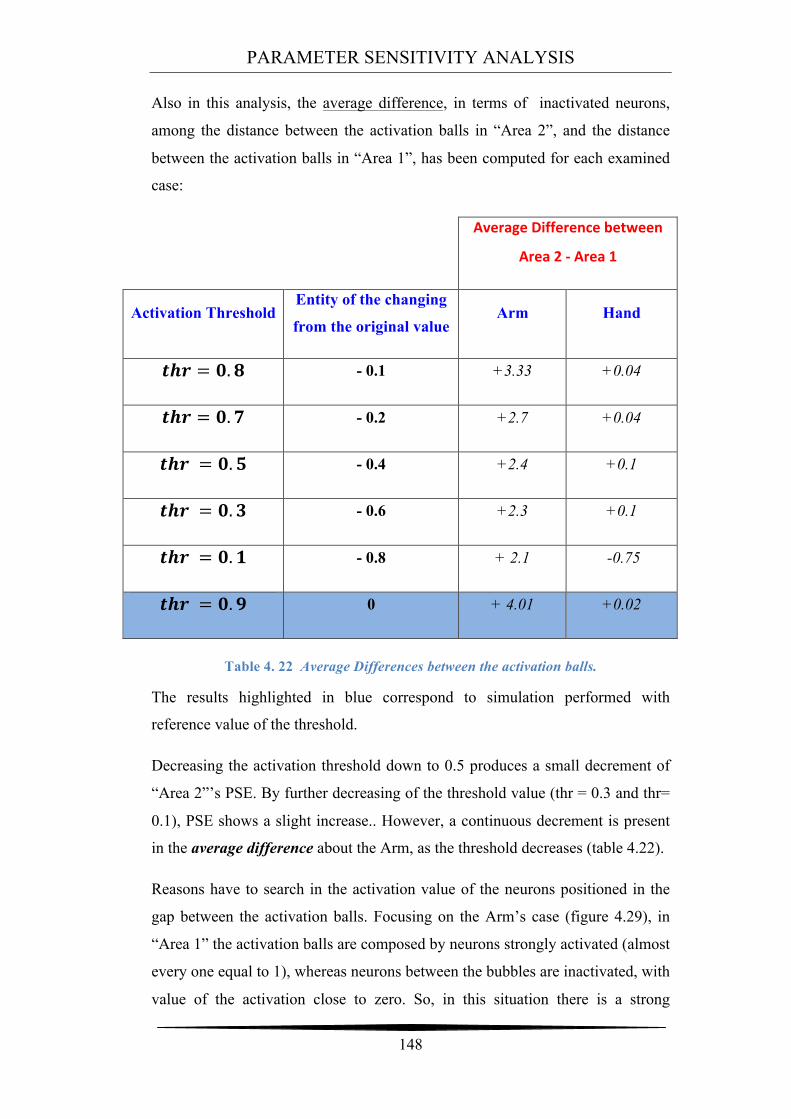
PARAMETER SENSITIVITY ANALYSIS
148
Also in this analysis, the average difference, in terms of inactivated neurons,
among the distance between the activation balls in “Area 2”, and the distance
between the activation balls in “Area 1”, has been computed for each examined
case:
Average Difference between
Area 2 -‐ Area 1
Activation Threshold Entity of the changing
from the original value Arm Hand
!"# = !.! - 0.1 +3.33 +0.04
!"# = !.! - 0.2 +2.7 +0.04
!"# = !.! - 0.4 +2.4 +0.1
!"# = !.! - 0.6 +2.3 +0.1
!"# = !.! - 0.8 + 2.1 -0.75
!"# = !.! 0 + 4.01 +0.02
Table 4. 22 Average Differences between the activation balls.
The results highlighted in blue correspond to simulation performed with
reference value of the threshold.
Decreasing the activation threshold down to 0.5 produces a small decrement of
“Area 2”’s PSE. By further decreasing of the threshold value (thr = 0.3 and thr=
0.1), PSE shows a slight increase.. However, a continuous decrement is present
in the average difference about the Arm, as the threshold decreases (table 4.22).
Reasons have to search in the activation value of the neurons positioned in the
gap between the activation balls. Focusing on the Arm’s case (figure 4.29), in
“Area 1” the activation balls are composed by neurons strongly activated (almost
every one equal to 1), whereas neurons between the bubbles are inactivated, with
value of the activation close to zero. So, in this situation there is a strong
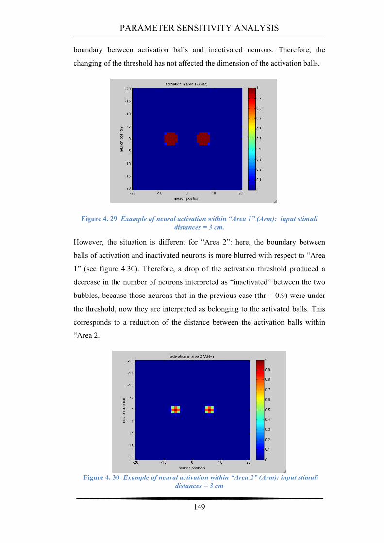
PARAMETER SENSITIVITY ANALYSIS
149
boundary between activation balls and inactivated neurons. Therefore, the
changing of the threshold has not affected the dimension of the activation balls.
Figure 4. 29 Example of neural activation within “Area 1” (Arm): input stimuli distances = 3 cm.
However, the situation is different for “Area 2”: here, the boundary between
balls of activation and inactivated neurons is more blurred with respect to “Area
1” (see figure 4.30). Therefore, a drop of the activation threshold produced a
decrease in the number of neurons interpreted as “inactivated” between the two
bubbles, because those neurons that in the previous case (thr = 0.9) were under
the threshold, now they are interpreted as belonging to the activated balls. This
corresponds to a reduction of the distance between the activation balls within
“Area 2.
Figure 4. 30 Example of neural activation within “Area 2” (Arm): input stimuli
distances = 3 cm
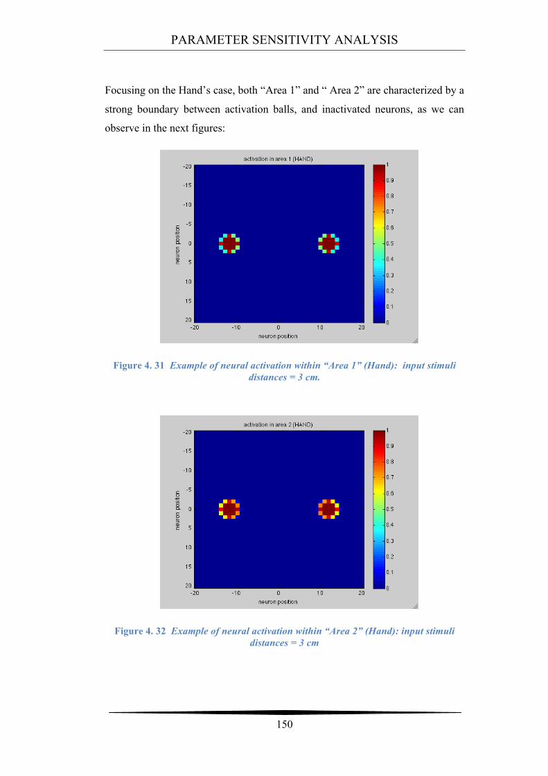
PARAMETER SENSITIVITY ANALYSIS
150
Focusing on the Hand’s case, both “Area 1” and “ Area 2” are characterized by a
strong boundary between activation balls, and inactivated neurons, as we can
observe in the next figures:
Figure 4. 31 Example of neural activation within “Area 1” (Hand): input stimuli distances = 3 cm.
Figure 4. 32 Example of neural activation within “Area 2” (Hand): input stimuli distances = 3 cm
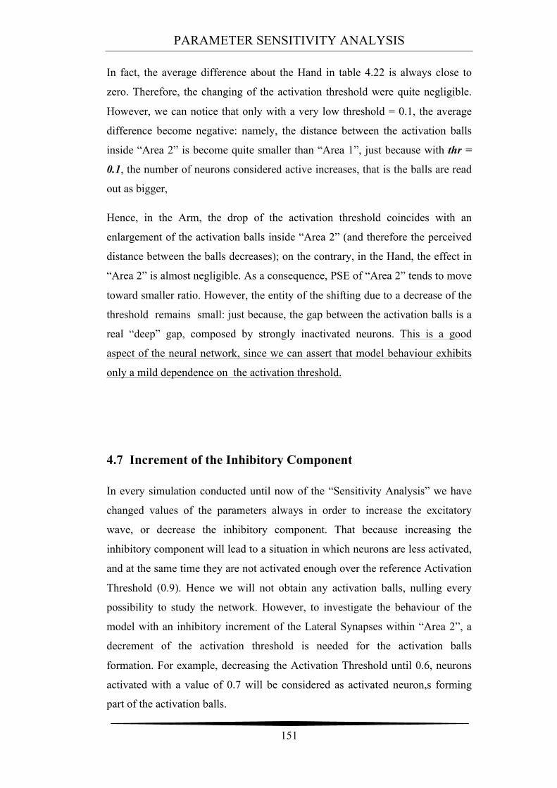
PARAMETER SENSITIVITY ANALYSIS
151
In fact, the average difference about the Hand in table 4.22 is always close to
zero. Therefore, the changing of the activation threshold were quite negligible.
However, we can notice that only with a very low threshold = 0.1, the average
difference become negative: namely, the distance between the activation balls
inside “Area 2” is become quite smaller than “Area 1”, just because with thr =
0.1, the number of neurons considered active increases, that is the balls are read
out as bigger,
Hence, in the Arm, the drop of the activation threshold coincides with an
enlargement of the activation balls inside “Area 2” (and therefore the perceived
distance between the balls decreases); on the contrary, in the Hand, the effect in
“Area 2” is almost negligible. As a consequence, PSE of “Area 2” tends to move
toward smaller ratio. However, the entity of the shifting due to a decrease of the
threshold remains small: just because, the gap between the activation balls is a
real “deep” gap, composed by strongly inactivated neurons. This is a good
aspect of the neural network, since we can assert that model behaviour exhibits
only a mild dependence on the activation threshold.
4.7 Increment of the Inhibitory Component
In every simulation conducted until now of the “Sensitivity Analysis” we have
changed values of the parameters always in order to increase the excitatory
wave, or decrease the inhibitory component. That because increasing the
inhibitory component will lead to a situation in which neurons are less activated,
and at the same time they are not activated enough over the reference Activation
Threshold (0.9). Hence we will not obtain any activation balls, nulling every
possibility to study the network. However, to investigate the behaviour of the
model with an inhibitory increment of the Lateral Synapses within “Area 2”, a
decrement of the activation threshold is needed for the activation balls
formation. For example, decreasing the Activation Threshold until 0.6, neurons
activated with a value of 0.7 will be considered as activated neuron,s forming
part of the activation balls.
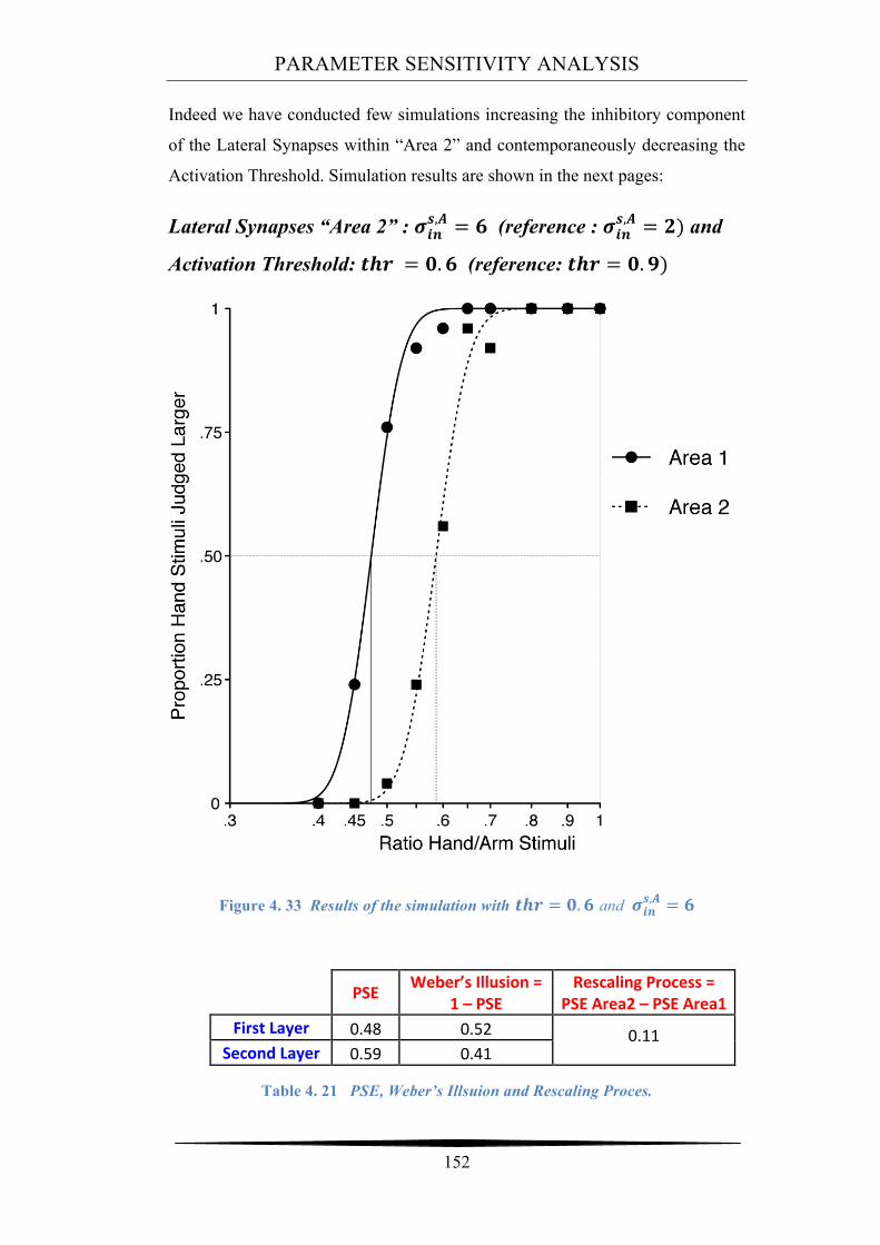
PARAMETER SENSITIVITY ANALYSIS
152
Indeed we have conducted few simulations increasing the inhibitory component
of the Lateral Synapses within “Area 2” and contemporaneously decreasing the
Activation Threshold. Simulation results are shown in the next pages:
Lateral Synapses “Area 2” : !!"!,! = ! (reference : !!"
!,! = !) and
Activation Threshold: !"# = !.! (reference: !"# = !.!)
Figure 4. 33 Results of the simulation with !"# = !.! and !!"!,! = !
PSE Weber’s Illusion = 1 – PSE
Rescaling Process = PSE Area2 – PSE Area1
First Layer 0.48 0.52 0.11 Second Layer 0.59 0.41
Table 4. 21 PSE, Weber’s Illsuion and Rescaling Proces.
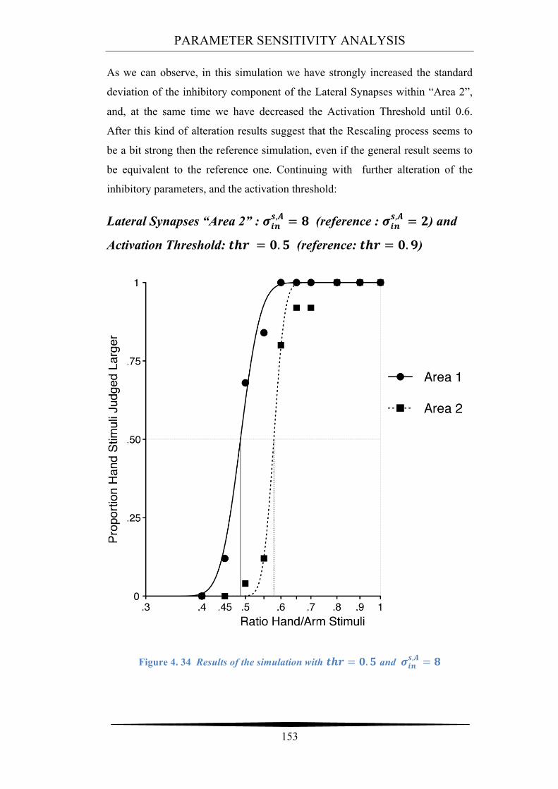
PARAMETER SENSITIVITY ANALYSIS
153
As we can observe, in this simulation we have strongly increased the standard
deviation of the inhibitory component of the Lateral Synapses within “Area 2”,
and, at the same time we have decreased the Activation Threshold until 0.6.
After this kind of alteration results suggest that the Rescaling process seems to
be a bit strong then the reference simulation, even if the general result seems to
be equivalent to the reference one. Continuing with further alteration of the
inhibitory parameters, and the activation threshold:
Lateral Synapses “Area 2” : !!"!,! = ! (reference : !!"
!,! = !) and
Activation Threshold: !"# = !.! (reference: !"# = !.!)
Figure 4. 34 Results of the simulation with !"# = !.! and !!"!,! = !
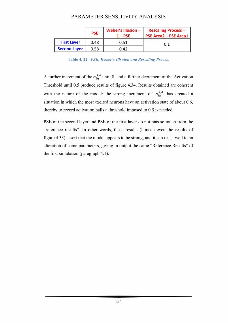
PARAMETER SENSITIVITY ANALYSIS
154
PSE Weber’s Illusion = 1 – PSE
Rescaling Process = PSE Area2 – PSE Area1
First Layer 0.48 0.51 0.1 Second Layer 0.58 0.42
Table 4. 22 PSE, Weber’s Illsuion and Rescaling Proces.
A further increment of the !!"!,! until 8, and a further decrement of the Activation
Threshold until 0.5 produce results of figure 4.34. Results obtained are coherent
with the nature of the model: the strong increment of !!"!,! has created a
situation in which the most excited neurons have an activation state of about 0.6,
thereby to record activation balls a threshold imposed to 0.5 is needed.
PSE of the second layer and PSE of the first layer do not bias so much from the
“reference results”. In other words, these results (I mean even the results of
figure 4.33) assert that the model appears to be strong, and it can resist well to an
alteration of some parameters, giving in output the same “Reference Results” of
the first simulation (paragraph 4.1).
155
CONCLUSIONS
The same distance between two punctual stimuli applied on the body surface is
perceived different across the body surfaces, an illusion known as Weber’s
Illusion (from the name of the researcher who first described such effect in the
scientific literature). The differences in receptors density across body regions,
and the distorted body image inside the Primary Somatic Sensory Cortex
(homunculus) are good starting points to investigate the Weber’s Illusion.
However, it seems not sufficient to consider only these aspects. Indeed
experimental results conducting along the last 100 years about this illusion have
led to the idea that higher order cortical areas, and other mechanisms are
involved in the perception of tactile distance. This idea has mainly arisen from
the observations that the illusion is much smaller than the differences in receptor
density, or cortical extent. Hence, perception of tactile distance might involve
cortical areas that operate a sort of “Rescaling Process” able to reduce this
illusion toward a verisimilar perception.
In the present thesis, we have tried to reproduce this illusion, by means of a
neural network model. The model is composed of two layers of neurons, able to
simulate the perception of the tactile distance between two punctual stimuli
applied on a virtual skin surface. In particular, we have simulated two different
body regions characterized by different receptor density and cortical
magnification (as the Hand and the Arm), in order to reproduce the Weber’s
Illusion as it was descripted in literature. This project wishes to provide insight
into the functional mechanisms that lie under the tactile perception, especially
tactile distance perception, and not to replicate physiologic and anatomic details.
The development of the neural network (in MATLAB environment) was based
on some simplification hypothesis. First, the presence of just two layers of
neurons: the “First Layer” considered as representing a part of the Primary
CONCLUSIONS
156
Somatic Sensory Cortex, receiving directly inputs from the stimuli applied on
the skin; and the “Second Layer”, considering as representing as higher cortical
areas. The second hypothesis concerns the role of these two layers: the first layer
was interpreted as the one affected by the Cortical Magnification as it occurs in
the primary somatosensory cortex, whereas the second layer as the area
providing the rescaling process, that is where distortions in tactile distance
perception occurring in the first layer are party compensated. The two layers are
connected by Feed-Forward synapses; moreover Lateral Synapses are present
inside each layer. Each neuron in the first layer is characterized by a tactile
Receptive Field; the RFs size on the simulated hand, was implemented smaller
than on the simulated Arm, in order to reproduce the higher tactile resolution in
the Hand compared to the Arm. Another important hypothesis introduced in the
model concerns how we read out network output. Indeed, in order to assess
network behaviour in terms of tactile distance perception, we need a quantity
that represents distance perception starting from the neuron population activity.
The simulation of two punctual stimuli on the skin surface produces a typical
pattern of neural activation inside the two layers, with the formation of two balls
of activated neurons within each layer. We have hypothesized that the perceived
distance might be read out as the number of inactivated neurons between the two
activation balls.
The so developed model is able to reproduce the Weber’s Illusion in which for
example, the same input stimuli distance applied first on the Hand, and then on
the Arm, was perceived different. Conducting many simulations with different
pairs of distances applied on the two body regions, we have computed the
perceived distance considering only the “First Layer”, and then the perceived
distance at the “Second Layer” (resulting from the interaction between the tow
layers). Results have shown that considering only the processing in the “First
Layer”, the Point of Subjective Equality (PSE) (i.e. the point at which the
applied distance on the hand is judged equal to the applied distance on the arm)
was quite small, equal to 0.48 (this means that, to perceive the same distance on
the two body regions, the actual distance on the arm must be more than double
than the actual distance on the hand). Considering also the processing in the
“Second Layer”, the illusion is reduced and the PSE is increased up to 0.6.
CONCLUSIONS
157
Notice that in the ideal case (no Illusion) the PSE should be equal to 1.
Therefore, the illusion (or distortion) was reduced of about the 20% within the
“Second Layer”. Value of PSE obtained in the “Second Layer” of the model
(0.6) is similar to the PSE obtained in experiments conducted of real subject,
(see Green’s paper in which PSE is equal 0.62); hence, the model reproduces
quite well the experimental data.
Furthermore, the neural network is able to reproduce another results of
experimental literature. In fact, real data about the hand and arm, show that there
is an almost linear function (with a positive slope) between real applied distance
and perceived distance, and that these functions on the two body parts tend to
diverge as applied distance increases. This means that as the applied distance
increases, the distance perception on the two body regions tends to become more
and more different. These results can be replicated with the neural network
model; this may further validate model architecture and assumptions. In fact the
output of the model suggest that for big input stimuli distances the Weber’s
Illusion increase, and at the same time we have recorded a decrement of the
Rescaling Process. This suggests us a possible explanation for the phenomena in
which the Weber’s Illusion increases as the stimuli dimension increase.
Moreover, model results about the two point discrimination thresholds on the
simulated Hand and Arm are coherent with the in vivo experimental results:
indeed, the neural network gave a smaller threshold for the hand with respect to
the arm. In fact, acuity of the hand in the perception of two nearby stimuli is
higher than on the arm, hence the two point discrimination threshold of the hand
is smaller than on arm.
Finally, the neural network has been demonstrated to be robust against variations
in some model parameters: in particular in the changing of the intensity of the
synapses connections (for both Feed-Forward synapses and Lateral Synapses)
and even the variation of the Activation Threshold. In particular, in the
simulation in which we have increased the inhibitory component of the lateral
synapses within “Area 2”, and contemporaneously decreased the Activation
Threshold, we have recorded about the same results obtained with the
CONCLUSIONS
158
“Reference Parameters”: this means that the dependence of the model from the
Activation Threshold is not absolute. Conversely, the alteration of the std
(standard deviation) of the excitatory component (or even the inhibitory
component) in the Lateral synapses within the Second Layer has produced a
dramatic changing in the mechanism of the Rescaling Process, nulling the
rescale effect. For example, std increment of the excitatory component in the
Lateral Synapses within “Area 2”, put the network in conditions to compute a
PSE of the second Layer, equal to the “First Layer”: it is clear that in this
situation, the Rescaling Process is completely off. The same result could be
appreciated decreasing the std of the inhibitory component.
The present model, besides providing insights into the mechanisms of tactile
distance perception and Weber’s illusion, in perspective it might be of value to
make some predictions, which can be verified later, in vivo, by tactile
experiments on real subjects.
Furthermore, in future works, this model could be associated, and unified, with
the neural network implemented by my university mate Monti Luca, about the
effect of stimulus orientation on tactile distance perception, in order to create a
unique, more complete model to investigate the tactile distance illusion.
159
Bibliography
Ø Matthew R. Longo and Patrick Haggard: “Weber’s Illusion and Body
Shape: Anisotropy of Tactile Size Perception on the Hand”. Institute of Cognitive Neuroscience, University College London.
Ø BARRY G. GREEN: “The perception of distance and location for dual tactile pressures”. Princeton University, Princeton, New Jersey.
Ø MRIGANKA SUR, MICHAEL M. MERZENICH, AND JON H. KAAS: “Magnification, Receptive-Field Area, and ‘Hypercolumn’ Size in Areas 3b and 1 of Somatosensory Cortex in Owl Monkeys”. Departments of Psychology and Anatomy, Vanderbilt University, Nashville, Tennessee 37240; and the Coleman Laboratory, Departments of Otolaryngology and Physiology, University of California, San Francisco.
Ø Sidney Weinstein, Chapter 10: “Intensive and extensive aspects of tactile sensitivity as a function of body part, sex and laterality”.
Ø Marisa Taylor-Clarke, Pamela Jacobsen & Patrick Haggard: “Keeping the world a constant size: object constancy in human touch”.
Ø Principle of Neuroscience, KANDEL: “Chapter 22: The Bodily Senses”.
Ø Principle of Neuroscience, KANDEL: “Chapter 23: Touch”.

Acknowledgments
I want to say thank you to my professor Elisa Magosso since she gave me the possibility to make this thesis project at the Birkbeck, University of London, giving me the possibility to make a wonderful, and different study experience that I have never tried.
Another important acknowledgment is direct to Dr. Matthew Longo due to his huge contribute in the analyse of the model results, as well as for his big availability to follow us even outside the university, doing also a fantastic guide around London.
A very big thank you to my family, always ready to support me in every moment, and to help me every time that I needed. I love you!
Finally, I have to say thank you to my Italian University mates (especially Luca Monti) whose I have shared 5 years of joys and sorrows, as well as to my new International friends that I have met in London during this long experience: even if it will be difficult to meet you guys anymore, I will remember you guys forever, because this experience in London was especial and unique even due to your presence…
…Enrico
Related Documents