Perceived inflation under loss aversion

Department Economics and Politics

Perceived Inflation under Loss Aversion Lena Dräger Jan-Oliver Menz Ulrich Fritsche DEP Discussion Papers Macroeconomics and Finance Series 5/2011 Hamburg, 2011

Perceived Inflation under Loss Aversion

Lena Dräger∗

Jan-Oliver Menz∗∗

Ulrich Fritsche‡

October 26, 2011

Abstract

Building on Prospect Theory, we apply the concept of loss aversion

to the formation of inflation perceptions and test empirically for non-

linearities in the inflation-perceptions relation for a panel of 10 Euro

area countries. Specifically, under the assumption of loss aversion, in-

flation changes above a certain reference rate will be perceived more

strongly. Rejecting rationality of inflation perceptions in general under

symmetric loss and in a majority of cases under flexible loss functions,

panel smooth transition models give evidence of non-linearities in the

inflation perception formation regarding both actual inflation and time.

This result is confirmed by dynamic fixed effects estimates, where the

slope of the estimated value function is significantly steeper in the loss

region and the implied average reference inflation rate is found close

to 2%.

Keywords: Inflation Perceptions, Loss Aversion, Panel Smooth Tran-

sition Models, Dynamic Panel.

JEL classification: C33, D81, D82, E31.

∗Corresponding author: University of Hamburg.Email: [email protected] would like to thank Jörg Breitung, Michael Lamla, Thomas Maag, Jan-Egbert Sturmas well as seminar participants at the University of Zurich, the University of Hamburgand the 2010 MMF Conference for their very helpful comments on earlier drafts of thispaper and Ulrich Brandt, Torsten Osigus as well as Philipp Poppitz for excellent re-search support. All authors thankfully acknowledge financial support from the DeutscheForschungsgemeinschaft.

∗∗University of Hamburg, Email: [email protected]‡University of Hamburg & KOF Swiss Economic Instiute, ETH Zurich, Email:[email protected]

I

1 Introduction

When assessing macroeconomic models empirically, economists mostly useactual data as published by statistical institutes for the theoretical variablesin these models. However, there exists overwhelming empirical evidence thatpeoples’ knowledge and perception of these variables may deviate consider-ably from official statistical data and their underlying concepts, questioningthe rationality of agents widely assumed since Muth (1961). Instead, infla-tion perceptions can be regarded as “nowcasts”, as agents form beliefs overactual inflation on the basis of information currently available and poten-tially subject to biases.1

The gap between actual data and individuals’ perceptions raises importantpolicy questions. This is especially true for inflation. As argued by van derKlaauw et al. (2008), among others, if individuals have biased beliefs aboutinflation, this can seriously undermine the central bank’s credibility. Con-versely, a credible monetary regime can also influence inflation perceptions,for instance by creating a focal point at the inflation target.2 Furthermore,relating to the concept of money illusion3, the perception gap may lead todistortions in bargaining if individuals misperceive their actual real purchas-ing power. To assess the effectiveness of policy propositions suggested bymacroeconomic models, it is thus necessary to understand how people formperceptions about macroeconomic variables and how these perceptions in-fluence individual behavior.So far, the literature on the formation of inflation perceptions has mainlyfocused on one stylized fact, namely the observed jump in perceptions afterthe Euro cash changeover in 2002, whereas actual inflation continued to stayon a low level. Explanations for this jump range from price intransparencies(Dziuda and Mastrobuoni, 2009), difficulties in applying the conversion rates(Ehrmann, 2006), a perceptual crisis (Eife, 2006, Eife and Coombs, 2007, Ful-lone et al., 2007 and Blinder and Krueger, 2004), macroeconomic illiteracy(Del Giovane et al., 2008, Cestari et al., 2008), a media bias (Lamla andLein, 2008), and expectancy confirmation (Traut-Mattausch et al., 2004).

A number of papers furthermore analyze factors influencing perceived infla-tion in general. Del Giovane et al. (2008) design a detailed survey for Italianconsumers in 2006. The authors report asymmetries in perceived inflation,since respondents stating that they have observed price decreases over thelast five years report significantly lower inflation perceptions than those not

1See Blanchflower and Kelly (2008), Blinder and Krueger (2004), Jonung and Laidler(1988), Malgarini (2008), Curtin (2007) and van der Klaauw et al. (2008).

2Evidence for this channel has been found in inflation perception surveys for Sweden, seeBryan and Palmqvist (2005).

3See Fisher (1928) for the original contribution, and Shafir et al. (2004) and Fehr and Tyran(2007) for a Behavioral Economics perspective.

1

recalling any price decreases. Furthermore, survey responses suggest a strongimpact of socioeconomic factors on inflation perceptions. This is in line withfindings in Jonung (1981) who claims that inflation perceptions in Swedendiffer significantly between genders. Furthermore, in a recent survey, Jonungand Conflitti (2008) report differences between age, gender, occupational andregional groups with respect to opinions of the Euro currency, which mayalso be reflected in inflation perceptions.Lein and Maag (2011) analyze the formation of inflation perceptions for theEU and Sweden, using data from the Joint Harmonized EU Program of Busi-ness and Consumer Surveys and Sweden’s Consumer Tendency Survey. Theauthors reject rationality of perceptions, since quantified inflation percep-tions fail the rationality conditions of accuracy, unbiasedness and efficiency.They also find some evidence for the importance of frequently bought goods,and for the expectancy confirmation hypothesis in the Euro area after thecash changeover. This is in line with Döhring and Mordonu (2007), whoreport an influence of inflation expectations on perceptions in addition toactual inflation, estimating a dynamic panel model for the countries thatadopted the Euro in 2002.Following the deviation of perceived from actual inflation rates at the Eurocash changeover, Brachinger (2006, 2008) proposes an Index of Perceived In-flation (IPI) meant to capture movements in perceived inflation better thanusual CPI inflation. The IPI index is constructed under the assumptionthat agents perceive inflation according to behavioral patterns defined inProspect Theory by Kahneman and Tversky (1979) and Tversky and Kah-neman (1981, 1991). These include the concepts of loss aversion with respectto above-average inflation and the availability bias. Jungermann et al. (2007)perform an experimental study of the assumptions underlying the IPI index,and find evidence of a loss aversion parameter of about 2.4 However, theirapproach has been criticized by Hoffmann et al. (2006) for its use of arbitraryad hoc assumptions.

This paper adds to the literature as follows. Building on Prospect Theory byKahneman and Tversky (1979) and Tversky and Kahneman (1981, 1991), weempirically test for the existence of loss aversion with respect to a referenceinflation rate affecting the formation of inflation perceptions.5

Developed as an alternative decision theory under risk and uncertainty op-posed to traditional expected utility theory,6 Prospect Theory proposes thatindividuals code price changes and evaluate them against a reference price,

4This relates well to studies of loss aversion in other areas, where approximately the sameparameter has been found, see for example Tversky and Kahneman (1991), Hardie et al.(1993) and Rosenblatt-Wisch (2008).

5Note that this is one of the hypotheses underlying the construction of the IPI index inBrachinger (2006, 2008).

6See Starmer (2004) for an overview of developments in decision theory under risk.

2

where higher prices are perceived as losses and lower prices are perceived asgains. Since individuals display loss aversion, price increases are perceivedmore strongly than price decreases, the exact quantity being captured bythe loss aversion parameter. Note that Prospect Theory defines loss aver-sion with respect to prices, while we analyze loss aversion with respect toinflation. This implies that a certain inflation rate is deemed ‘normal’, whileinflation rates above the ‘normal’ rate are perceived as a loss. Also, analyzingloss aversion with respect to inflation entails a dynamic view of price devel-opments, where reference prices and the reference inflation rate are groundedin households’ historical experience (Malmendier and Nagel, 2011).7

Figure 1 shows a stylized value function describing the relation betweenperceived and actual inflation. The existence of loss aversion leads to a kinkat the reference rate of inflation, with a steeper slope in the loss region whereinflation rates are above the reference rate.8

< Figure 1 here >

We evaluate loss aversion regarding inflation by analyzing households’ sur-vey data on perceived inflation compiled by the European Commission inthe Joint Harmonized EU Program of Business and Consumer Surveys. Inorder to apply for rationality tests, and to allow for the estimation of in-terpretable slope parameters, the qualitative survey answers are quantifiedwith the method by Carlson and Parkin (1975), which has been adapted toa pentachotomous survey by Batchelor and Orr (1988). The sample thencovers a panel of 10 Euro area countries from January 1996 to December2010.The empirical investigation takes the following route: First, we examinerationality criteria for inflation perceptions following the seminal work ofMincer and Zarnowitz (1969) and test for the unbiasedness and efficiencyof perceived inflation. Underlying these rationality tests, however, is theassumption of a symmetric loss function, which is no longer appropriate ifloss aversion with respect to high inflation rates is present. Thus, we extendthe analysis by applying the quantile approach by Patton and Timmermann(2007), which accounts for both symmetric and asymmetric loss functions.9

Second, the existence and shape of a non-linear relation between perceived

7The concept of loss aversion has also been applied to other areas, such as brand choice orconsumption patterns, see for instance Hardie et al. (1993), Camerer (2000), Rosenblatt-Wisch (2008), Foellmi et al. (2011) and Gaffeo et al. (2011).

8In order to determine the reference price, two routes can be followed. In the contextof consumer choice, the reference price is given by the fair price, which is determinedby consumers’ perceptions of sellers’ costs. This idea has first been proposed by Thaler(1985) and recently been pursued further by Rotemberg (2005, 2008). With regard toinflation perceptions, Brachinger (2006) argues that one could simply take a past price asthe reference price. However, it is not clear whether one should use an average price of abundle of goods and how long the reference time period should be.

9A similar approach is followed by Capistrán and Timmermann (2009) who analyze asym-

3

and actual inflation is investigated in a Panel Smooth Transition (PSTR)setting proposed by Gonzalez et al. (2005) and Fok et al. (2005). Thisapproach allows the estimation of the reference inflation rate and the tran-sition function, while accounting for potential structural breaks. Finally, weestimate dynamic fixed effects models with threshold variables, defining atime-varying reference inflation rate, as a robustness check and in order todetermine the slope parameters and the location of the kink in a non-linearperception-inflation relation.Our analysis suggests the following results: While we generally reject ratio-nality of inflation perceptions in our sample, allowing for asymmetric lossfunctions yields a number of non-rejections in the second half of our sam-ple period. This indicative result of asymmetries underlying the inflation-perceptions nexus is further confirmed by the PSTR models, which findnon-linearities with respect to both actual inflation and time. Generally,results suggest a significantly stronger effect of actual inflation changes onperceptions once inflation is above a certain threshold, which is estimatedto be in the range from 1.8% to 3.3%. Estimates from dynamic fixed effectsmodels with a time-varying reference rate of inflation confirm this result andimply a reference rate close to 2%.The remainder of the paper is structured as follows. Section 2 describes thedata set, including the quantification method for the qualitative survey dataand presents panel unit root and cointegration tests. Section 3 proceeds withpresenting the estimation design, followed by a discussion of the results inSection 4. Finally, Section 5 concludes.

2 Data Set and Statistical Properties

2.1 Perceived and Actual Inflation

The hypothesis from Prospect Theory – there is a non-linear relationshipbetween perceptions and inflation – is tested empirically for a panel of 10EMU-Countries consisting of Austria, Belgium, Finland, France, Germany,Greece, Italy, the Netherlands, Portugal, and Spain for the time period fromJanuary 1996 to December 2010. Our sample thus covers the Euro areaalmost completely, and the sample period is long enough to enable us to testfor possible structural breaks.We use a quantified version of the balance statistic of Question 5 of theJoint Harmonized EU Program of Business and Consumer Surveys by theEuropean Commission as our measure of perceived inflation. The officiallypublished balance statistic of the survey provides only a qualitative measurefrom the pentachotomous survey, asking participants whether they think

metries regarding the formation of inflation expectations from the Survey of ProfessionalForecasters in the US.

4

prices have fallen/ stayed about the same/ increased at a slower rate/ in-creased at the same rate/ increased more rapidly over the last 12 months.Denoting the shares of answers in each category as s1, s2, s3, s4 and s5, thebalance statistic is obtained as s1 + 0.5s2 − 0.5s4 − s5. While most em-pirical studies on perceived or expected inflation with data from the JointHarmonized EU Program of Business and Consumer Surveys make use ofthe balance statistic, there exist methods to quantify the qualitative data.Given that we want to test the rationality of perceptions under symmetricor asymmetric loss functions explicitly, we have to rely on quantified percep-tion data. We thus follow Döpke et al. (2008) and employ a version of theprobability method proposed by Carlson and Parkin (1975) and modified byBatchelor and Orr (1988).10

The quantification method demands a scaling series that inflation percep-tions are assumed to be based upon. We specifically assume that householdsobserve the underlying medium-term trend of the true inflation rate cor-rectly and proxy the current scaling value of inflation with a recursivelyestimated Hodrick-Prescott filter under the usual assumption of λ = 14.400for monthly data. Business cycle fluctuations are therefore excluded fromthe expected value observed by households. Details are explained in thetechnical appendix of this paper (section A).11

Actual inflation rates are measured with annual inflation rates of harmonizedconsumer price indices (HICP) from Eurostat. All data are available on amonthly basis. Figure 2 shows the quantified perceptions together with theinflation rates for all countries of our sample. In most countries of oursample, on average quantified perceptions track actual inflation relativelyclosely. Nevertheless, significant deviations do occur, for instance at theEuro cash changeover or at the spike in inflation before the financial crisis.

< Figure 2 here >

2.2 Unit Roots and Cointegration

We test the time series of actual and perceived inflation rates for panel unitroots in order to avoid spurious regressions. Details on the test statistics andresults are given in the appendix (section B). In line with results in the liter-ature, e.g. Lein and Maag (2011), we find that the null hypothesis of a unitroot in inflation is mostly rejected, while perceptions seem more persistent.Generally, empirical evidence on the order of integration of inflation series ismixed, Altissimo et al. (2006) conclude in a survey that empirical findings

10See also Nielsen (2003) for a survey.11See Nardo (2003) for a critical overview on quantification of survey data. Maag (2009)

analyses both quantitative and qualitative measures of Swedish inflation perceptions andexpectations. The author finds that quantified data and balance statistics are of equalaccuracy and that both are highly correlated with the mean of actual quantitative beliefs.

5

seem to lean towards stationarity of inflation. Due to the mixed results withrespect to stationarity of perceived and actual inflation rates, we proceed totest for panel cointegration between perceptions and inflation.A detailed description of the panel cointegration tests applied and of theresults is again given in the appendix. We find significant evidence for coin-tegration: For the whole sample period, all tests reject the null of no co-integration at the 1% level. This, quite intuitive, result is in line with find-ings in Lein and Maag (2011) for a similar sample. Considering the resultsfrom both panel unit root and cointegration tests, we estimate regressionsin the analysis in levels, making use of the super-consistency argument byEngle and Granger (1987).

3 Estimation Design

3.1 Non-Rationality of Perceived Inflation under Flexible

Loss Functions

The paper of Mincer and Zarnowitz (1969) on the empirical investigation ofthe rationality of professional forecasts initiated a bulk of literature on theeconometrics of rationality tests. These tests are regularly applied to infla-tion forecasts of professional forecasters and households. Under the assump-tion that aggregate information dissipates slowly throughout the economy(i.e. “sticky information”), households’ perceptions can be seen as forecastsmade today (so-called “nowcasts”), based on all the available information inthe current time period. Therefore, most rationality tests in the forecastevaluation literature can be applied to inflation perceptions as well. How-ever, rationality tests typically rely – implicitly or explicitly – on the axiomof a symmetric loss function (see Granger, 1969; Bachelor and Peel, 1998;Patton and Timmermann, 2007). The first class of such tests dates back tothe seminal paper of Mincer and Zarnowitz (1969) and is therefore calleda “Mincer-Zarnowitz regression”. The test is constructed as a joint test ofthe unbiasedness and efficiency of the forecast. Dufour (1981) and Campbelland Ghysels (1995) suggest non-parametric tests on both aspects based ona usual Wilcoxon-Sign-Rank-test (see Wilcoxon, 1945).12.The symmetric loss function might be a good approximation for a wide rangeof cases. However, asymmetric loss functions are also quite plausible and es-pecially suitable in cases where a loss aversion model is to be tested. To testfor rationality in a broader sense, we therefore use a more flexible approachand employ an indicator function (or quantile approach) as proposed by Pat-ton and Timmermann (2007). Under the joint assumption that the relevantloss is a function solely of the forecast error and that the functional form of

12We report results of non-parametric rationality tests based on a symmetric loss functionin the appendix (section C)

6

the loss function is homogenous in the forecast error, we can use an indicatorfunction which takes the value of one if the forecast is equal to or larger thanthe realization (i.e. the perception is higher than the true inflation rate) andestimate the following model:

It = α0 + α1ˆyt|t (1)

where ˆyt|t is the perception in time t. Patton and Timmermann (2007) showthat the indicator variable It should be independent of any element in theinformation set and therefore the restriction α0 = α1 = 0 should hold. Wereport results from a probit model which is satisfied due to the binary natureof the data.13

3.2 A Panel Smooth Transition Approach

Having tested for asymmetries in the inflation-perceptions relation in theprevious section, we proceed to investigate the (potentially nonlinear) rela-tionship further by applying the Panel Smooth Transition (PSTR) modeldeveloped by Gonzalez et al. (2005) and Fok et al. (2005). Recently, this ap-proach has been used in a number of applications. With its help, Hurlin andcoauthors investigate the nonlinear relationship between public capital andoutput (Colletaz and Hurlin, 2006), the Feldstein-Horioka puzzle (Fouquauet al., 2008), and energy demand (Destais et al., 2009). Others have used thePSTR-model to analyze nonlinearities with respect to health care expendi-ture and GDP (Chakroun, 2010, Mehrara et al., 2010), the effects of financialdevelopment and growth (Jude, 2010), and the link between inflation andgrowth (Ibarra and Trupkin, 2011).The increasing popularity of the PSTR-model might be due to the fact thatit has two advantages over simple fixed effects estimations.First, the model allows to explicitly test for nonlinearity, and to endogenouslydetermine both the threshold and the degree of nonlinearity. Second, as willbecome clear below, the PSTR-model also allows for different coefficientsof the explanatory variables over time and over cross-section units, whereasthe dynamic fixed effects model only captures panel heterogeneity by fixedindividual and time effects. One caveat applies, however. By now, it is stillunclear how the PSTR-model, and also the PTR-model proposed by Hansen(1999), behaves with respect to dynamic panels including lags of the endoge-nous variable. Given the high serial correlation of inflation perceptions, thisproblem deserves particular attention in our setting. Hence, we will presentPSTR estimates both including and excluding lagged inflation perceptionsfrom the nonlinear part, and also apply dynamic fixed effects. Moreover,

13We experimented a bit with the functional form of the underlying cumulative distribution.In most cases, logit models yield qualitatively similar results. Results are available fromthe authors upon request.

7

we estimate single country regressions using the Smooth Transition Autore-gressive (STAR)-model developed by Granger and Teräsvirta (1993) whichis able to deal with the existence of lagged endogenous variables.

Specifying and Estimating the Model

The PSTR-model, allowing for nonlinearities between the explanatory vari-ables and the dependent variable, and a smooth transition between differentregimes separated via a transition variable, is defined as:

yit = µi + β0x′it + β1x

′itG(qit; γ, c) + uit (2)

where t = 1, . . . , T and i = 1, . . . , N denote the time and the cross-sectiondimension, respectively, and µi captures the fixed individual effects. For G,one uses the logistic function

G(qit; γ, c) =

1 + exp

−γG

m∏

j=1

(qit − cj)

−1

, (3)

Here, qit is the transition variable: in case we find a nonlinear relationship,the coefficients of the explanatory variables change in line with the valueof the transition variable. c = (c1, . . . , cm)′ is an m-dimensional vector oflocation parameters, i.e. the number of thresholds and regimes. For example,if m = 1, we have one threshold, and two regimes, whereas for m = 2,the model consists of three regimes, a middle one, and two identical outerregimes. Finally, γ defines the steepness of the transition function, i.e., withγ = 0 we are back to the linear model, and with γ → ∞, the model tends toa regime-switching model as developed by Hansen (1999).This model can be understood in two ways. First, it can be interpretedas a regime-switching model, in which we get one coefficient β0 in regimeone, and another coefficient β0 + β1 if we are in regime two. Observationsare divided into regimes via the transition variable qit, and the transitionbetween regimes might be smooth or immediate, depending on the value ofγ. However, the model can also be seen as allowing for a large number ofsmall regimes, each one being determined by a specific value of the transitionvariable. Applied to our research question: If individuals consider inflationdifferently depending on whether it is above or below a certain threshold, wewill have a two-regime model, high- and low-inflation. By contrast, we couldalso interpret the findings in such a way that individuals adjust smoothlyto changes in the inflation rate, resulting in various inflation/perception-regimes.The PSTR-model can also be extended to allow for more than one transitionfunction, in order to capture larger degrees of nonlinearity:

8

yit = µi + β0x′it +

r∑

j=1

βjx′itGj

(

q(j)it ; γj , cj

)

+ uit (4)

where r is the number of transition functions. If r = 0, we are back to thelinear model. Moreover, this latter specification can be used to test for a(gradual or immediate) structural break.14 This is done by using a secondtransition function

T (t∗; γ, c) =

1 + exp

−γT

h∏

j=1

(t∗ − cj)

−1

(5)

with the time index t∗ = t/T as additional transition variable.Summing up, this model allows for a number of possible relationships be-tween the variables of interest. Applied to our research question regardingthe link between inflation perceptions and the actual inflation rate, we wouldexpect a model with m = 1 and r = 1, i.e. a model with one threshold (thereference inflation rate), two regimes (one above and one below the referencerate), and with one transition function. In case we find a structural break,we might get a model with r=2 and two different transition variables, theinflation rate and the time dimension.Before estimating the model, we have to determine the number of locationparameters m, and the number of transition functions.15

We start by testing H0 : r = 0 vs. H1 : r = 1: If we do not reject the nullhypothesis, we conclude that the relationship is in fact linear, and estimatea dynamic fixed effects model. If we reject the null, we continue with testingH0 : r = 1 vs. H1 : r = 2, i.e., we test for remaining non-linearity. Werepeat this procedure until we cannot reject the null hypothesis anymore,ending up with the optimal number of transition functions. The tests arecarried out by replacing G(qit; γ, c) in (2) by its first-order Taylor expansionaround γ = 0. Hence, one estimates the auxiliary regression

yit = µi + β∗0x

′it + β∗

1x′itqit + β∗

2x′itq

2it + . . .+ β∗

mx′itqmit + u∗it (6)

where the vectors β∗1 , . . . , β

∗m are multiples of γ. Thus, testing H0 : β∗

1 =. . . = β∗

m = 0 is equivalent to testing H0 : γ = 0 in (2), in which case themodel collapses into a standard linear fixed effects panel regression.Next, estimation is carried out in three steps.16 First, the individual ef-fects µi are removed by subtracting the individual-specific means. Then,initial values for γj and cj are chosen by means of a grid search, and, given

14See Gonzalez et al. (2005).15See for details Colletaz and Hurlin (2006).16We use the RATS code developed by Gilbert Colletaz and Christophe

Hurlin that the authors have kindly made available online, seehttp://www.univ-orleans.fr/deg/masters/ESA/GC/gcolletaz_R.htm.

9

these values, the coefficients βj are estimated with OLS. Third, using theseestimates, γj and cj are estimated by nonlinear least squares, allowing tocalculate the final estimates for βj . After the estimations, information cri-teria are compared in order to determine the optimal number of locationparameters.Concerning the interpretation of the estimated parameters, we can calculatethe partial derivatives as

eit =∂yit∂xit

= β0 +

r∑

j=1

βjG(qit; γj , cj) (7)

or, if the threshold variable is the same as the explanatory variable, as:

eit =∂yit∂xit

= β0 +r

∑

j=1

βjGj(qit; γj , cj) +r

∑

j=1

βjxit∂Gj(qit; γj , cj)

∂xit(8)

It is important to note that these derivatives cannot directly be interpretedas elasticities, given that their value depends on G(qit; γ, c). More precisely,if the transition function tends either to 0 or to 1, we can determine theelasticities in the extreme regimes, β0 and β0 + β1. However, given that thetransition between regimes might be smooth, we receive a number of elastic-ities defined as a weighted average of the extreme values. This means thatthe PSTR-model allows for different coefficients of the explanatory variablesfor each country over time: In each period, and for each individual country,the transition function takes on a different value resulting in a specific valuefor the elasticity.Besides these time-varying and individual-specific coefficients, we can inter-pret the signs of the estimated parameters. If β1G is found to be positive,this means that the estimated effect from inflation on perceptions rises withthe inflation rate, i.e., the higher the level of the inflation rate, the strongerthe impact of a one percentage point increase on inflation perceptions.

Estimated Models

Using the inflation rate and time as transition variables, and the entire dataset 1996m01–2010m12, we first test for nonlinearity with respect to bothtransition variables. This takes into account the structural break betweeninflation perceptions and inflation around the Euro cash changeover in Jan-uary 2002, which has been documented by a number of researchers.Hence, in case we find nonlinearity, we estimate the following model:

πpi,t = µi + α0π

pi,t−1 + β0πi,t + β1πi,tG(γ1, cm,1, πi,t)

+ β2πi,tT (γ2, cm,2, t∗) + εi,t (9)

10

For the sake of comparison, we re-estimate the model using lagged inflationperceptions also in the non-linear part.

πpi,t = µi + α0π

pi,t−1 + β0πi,t +

[

α1πpi,t−1 + β1πi,t

]

G(γ1, cm,1, πi,t)

+[

α2πpi,t−1 + β2πi,t

]

T (γ2, cm,2, t∗) + εi,t (10)

Depending on whether we find one or two regimes (m = 1, or m = 2), thetransition functions become:

G(c1)/T (c1) = (1 + exp(−γ1(qit − c1)))−1 (11)

G(c1, c2)/T (c1, c2) = (1 + exp(−γ1(qit − c1) · (qit − c2)))−1 (12)

3.3 Dynamic Fixed Effects

After testing for a non-linear relation between perceived and actual infla-tion in a general panel smooth transition setting, we estimate the changein the slope of the value function, as well as the change in the intercept,in a dynamic panel fixed effects model. Note that applying the well-knowndynamic panel estimator to our model also allows us to check for robustnessof the PSTR results, where so far applicability to models including a laggedendogenous term has not been thoroughly investigated.Assuming that the transition from the “gain” to the “loss” region takes theform of a kink as in Figure 1, we construct two threshold-dummies that serveto capture the periods where losses in the form of rising inflation occurred. Ifthe hypothesis of loss aversion holds, we should find a significantly strongerimpact of those “loss” periods on perceived inflation than of the “gain” periodsin inflation. The threshold-dummies for all i = 1, 2, ..., 10 countries in thepanel are defined as follows:

thold1,it =

1 if πit > πMAit

0 otherwise,

thold2,it =

1 if πit > πHPit

0 otherwise,

where πMAit represents a 13-months backward-looking moving-average of in-

flation and πHPit stands for recursively HP-filtered inflation. We thus assume

that the medium-term trend in inflation is observed correctly and servesas the time-varying reference inflation rate. This is in line both with ourassumption for the quantification procedure and with the theoretical argu-ment that loss aversion regarding inflation implies a dynamic view on theperception of prices and, thus, calls for a reference rate grounded in histori-cal experience. The threshold dummies take on the value of one for periodswith above-average inflation, and zero otherwise.

11

The threshold-dummies are then included in a dynamic fixed effects modelof inflation perceptions, both individually and combined with HICP inflationrates. Thereby, we can account both for a change in the slope parameterand for a change in the intercept during periods with above-average inflationrates. We thus estimate the following model:17

πpit = α0+α1thold1,2it+α2π

pit−1+β1πit+β2(πit ∗ thold1,2it)+γi0+ εit (13)

A significantly positive coefficient β2 in equation (13) suggests higher per-ceived inflation rates in periods of above-average inflation for our panel and,thus, gives evidence of loss aversion with respect to inflation. Regarding thechange in the intercept captured by α1, if we expect the reference rate ofinflation to be positive, the kink should lie above the origin and the interceptfor “loss” periods α1 would be below the normal intercept due to the steeperslope of the value function in the loss region. In the presence of loss aversion,we thus expect β2 to be significantly positive and α1 significantly negative.Note that equation (13) models loss aversion with respect to inflation as along-run phenomenon, in line with the theory in Kahneman and Tversky(1979).

4 Results

4.1 Rationality Tests under Flexible Loss Functions

Evaluating rationality of inflation perceptions under a wide range of lossfunctions, we report results of the quantile test for rationality introduced byPatton and Timmermann (2007).18 The results in Table 1 indicate that evenunder the mild assumptions of the test used here, the null of rationality hasto be rejected in almost all cases if we test over the full sample period.However, visual inspection as well as the results of formal structural breaktests reported later in the paper, lead us to conclude that at least one oreven two sample splits might be necessary to control for breaks. Interest-ingly, the results change to some extent once we control for structural breakseither around the Euro cash changeover or around the spike in inflation ratesshortly before the financial crisis turmoil. Especially if we control for the cashchangeover break, the number of rejections drop significantly. This is in con-trast to the well-known results from traditional Mincer-Zarnowitz regressionsand other rationality tests based on the symmetric loss assumption, which

17We tested for possible endogeneity of inflation rates in equation (13), but found no corre-lation between πit and εit in any of the specifications.

18Results of non-parametric rationality tests under the symmetric loss assumption as inCampbell and Ghysels (1995) are given in the appendix of this paper in section C. Furtherresults of tests in the spirit of Mincer and Zarnowitz (1969) are available from the authorsupon request.

12

uniformly reject the rationality of inflation perceptions (Jonung and Laidler,1988; Lein and Maag, 2011; Dräger, 2011). We interpret this as a hint thatthe result of “non-rationality” observed in other studies might to some extentbe driven by asymmtric loss functions, due for instance to loss aversion.

< Table 1 here >

4.2 Panel Smooth Transition Regression

Next, we turn to the results of the Panel Smooth Transition Model. Begin-ning with the linearity tests shown in Table 2, we note that linearity withrespect to inflation is rejected if we allow for two thresholds (m=2), butnot for models with only one threshold. However, if we turn to test thenull hypothesis of one transition function (r=1) against the alternative ofat least two nonlinear functions, the null is also rejected for a model withone threshold.19 This seemingly contradictory result might be due to thestructural break around the Euro cash changeover (see below), a fact that issupported by the strong rejection of linearity with respect to time. Hence, wecontinue to estimate models with one transition function for each transitionvariable inflation and time.

< Table 2 here >

Next, we have to decide on the optimal number of thresholds, m. Table3 displays the information criteria and the residual sum of squares (RSS)for different specifications. We use time as second transition variable, anddistinguish between models with one and two thresholds (1,1 and 2,2), inaddition to only one threshold for inflation and two thresholds for time (1,2).The results are fairly clear-cut. Regarding the model with only inflation inthe nonlinear part, both the AIC and the Schwarz criterion prefer the modelwith m = (1, 2). By contrast, allowing for lagged inflation in the nonlinearpart, the information criteria choose m = (1, 1) as the best specification.Hence, based on the test results, we continue to estimate (1, 1)- and (1, 2)-models for both linear and nonlinear lagged perceptions.20

< Table 3 here >

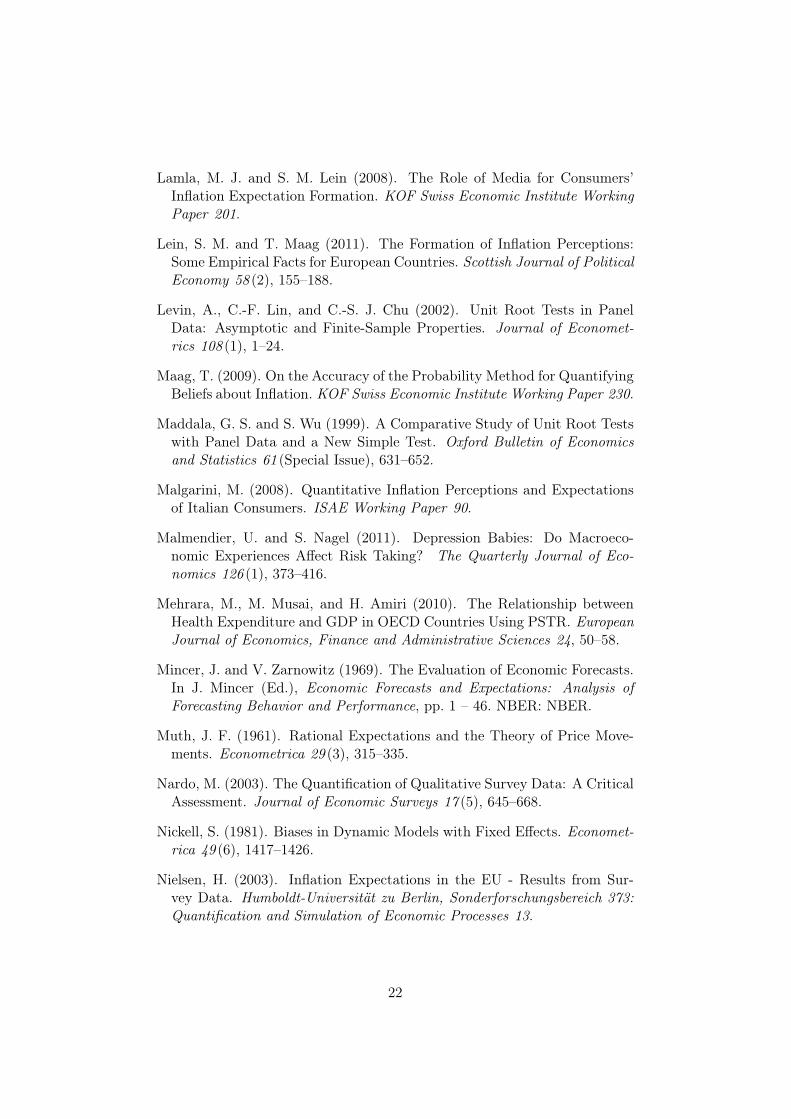
The resulting parameter estimates are given in Table 4. As it turns out,the results are fairly similar across the different specifications. With regard

19Restricting lagged perceptions to be linear does not allow to test for more than one tran-sition function.

20As noted by Gonzalez et al. (2005), the test results have to be interpreted with cau-tion, since the results are influenced by cross-country heteroscedasticity which cannot beaccounted for yet. Hence, we do not a priori refrain from estimating the (1, 1)-model,however, we are confident to exclude the (2, 2)-specification given that in this case, theconvergence of the algorithm is largely dependent on the starting values of the grid search.

13

to time, we always find large γT′s pointing to the existence of at least one

structural break. The associated thresholds 0.4 and 0.8 roughly belong toJanuary 2002, the date of the Euro cash changeover, and to July 2008, thebeginning of the financial crisis. Concerning the steepness of the transitionfunction using inflation as threshold variable, we get γG

′s between 0.8 and2.2, however, the two lowest values estimated for the model using nonlinearlagged perceptions are not significantly different from zero. The associatedthreshold inflation rates range from 1.8% to 3.3%. Next, we find inflationperceptions to be quite persistent with estimates of their lagged value closeto 0.9.Regarding the effect from actual inflation on perceptions, we thus do findsupport for loss aversion with respect to high inflation rates: All nonlinearcoefficients πtG are significantly positive, meaning that individuals perceivechanges in inflation more strongly if inflation is above a certain threshold.Moreover, the coefficient with respect to time πtT suggests that this effecteither increased after the Euro cash changeover, or that the effects havebeen lower before the Euro cash changeover and after the beginning of thefinancial crisis.

< Table 4 here >

Note that these findings are also supported by the individual STAR regres-sions that we have estimated as robustness checks for the time span 2002m1–2010m12.21 The estimated thresholds lie between 2.5% and 3.5%, with theexception of Spain where we estimate a threshold of 4%. Moreover, in caseof Austria, Belgium, Finland, France, Germany, Italy, and Portugal, we findrather large γG

′s, and positive coefficients for inflation in the nonlinear part.Finally, we illustrate the differences in the effects of actual inflation on per-ceived inflation over time and between countries. For that purpose, Figure3 shows scatter plots of actual inflation and the country- and time-specificelasticities computed according to equation (8) for the PSTR-model allow-ing only for the structural break at the Euro cash changeover.22 The blackline shows the relationship after the Euro cash changeover, and the gray linethe link for the period before. For all countries, we can observe a nonlinear,smooth relationship between actual inflation and the elasticities. Besides, thefigures show an upward shift in the turning point of the transition function inAustria, France, and Germany; a hint that in those countries, the referencerate of inflation might have increased after the Euro cash changeover.

< Figure 3 here >

21The detailed results are available upon request. Prior to the Euro introduction, the resultsare not reliable due to the short sample period.

22Allowing for the second structural break at the time of the financial crisis yields qualita-tively similar results.

14

4.3 Dynamic Fixed Effects Estimations of Loss Aversion

Finally, we present results of the panel estimation of loss aversion as inequation (13) with both threshold dummies in Table 5, where the first columnadditionally reports a test for adaptive perceptions.

< Table 5 here >

Due to our finding of cointegration between actual and perceived inflation,we estimate all equations in levels, using dynamic fixed effects to account forthe high degree of persistence in perceived inflation. Even if this estimatorsuffers from the Nickell (1981) bias, this is not a severe problem since T issignificantly larger than N in our sample. For the same reason, the Arellanoand Bond (1991) estimator would be computationally inefficient. Hence, weemploy the dynamic fixed effects estimator and check for a possible influencefrom the Nickell bias by using the ‘Least Squares Dummy Variable Corrected’(LSDVC) estimator proposed by Bruno (2005).23 The results are robustacross all estimators. Additionally, conducting the Pesaran (2004) and theBreusch and Pagan (1980) tests of error cross-section dependence revealsthat residuals are correlated across panels.24 Hence, we present estimateswith correlated panels corrected standard errors.Estimation results from the PSTR model suggest the existence of two struc-tural breaks in the perception-inflation relation over our sample period,namely at the Euro cash changeover in January 2002 and at the onset ofthe financial crisis in July 2008. Therefore, we conduct Quandt-Likelihood-Ratio tests for single country estimations of the model in (13) with boththresholds. The test runs individual structural break tests over each monthin the full sample period and selects the date with the maximum Wald F-Statistic as the break date. Results presented in Table D.1 in the appendiximply that, over the full sample period, the structural break during themonths preceding the financial crisis dominates over the break at the Eurointroduction.25

We thus estimate the model in equation (13) over the full sample period1996m1–2010m12 and compare the results to estimates from a restrictedsample period 1996m1–2007m12, excluding the dominant break.26

Throughout all models, we find that lagged inflation perceptions yield ahighly significant coefficient of about 0.94–0.96. This suggests indeed a high

23Results are available from the authors upon request.24Test results are available from the authors upon request.25Restricting the sample period to 1996m1–2007m12, Quandt-Likelihood-Ratio tests identify

the second break at the Euro cash changeover in almost all sample countries. Results areavailable from the author upon request.

26We further estimated models accounting for the break in January 2002 by including adummy variable taking on the value of 1 for the months 2001m11–2002m2. However, thedummy was insignificant in all models and the coefficients remained robust. Estimationresults are available upon request.

15

degree of persistence in inflation perceptions; a results which was also im-plied by the panel unit root tests above. We thus cannot rule out thatinflation perceptions in our panel are to some degree formed adaptively. Inthe preliminary model without threshold dummies, the coefficient on actualinflation implies a long-run impact of 1.2 from actual to perceived inflation.Accounting for a possible effect of loss aversion on the perception-inflationrelation, both models for the full sample period yield a significant coeffi-cient β2, indicating that inflation indeed influenced perceptions significantlystronger in periods with above-average inflation rates. As expected, bothmodels also find a negative coefficient α1 for the intercept dummy thold1,2.However, only the model with thold2 constructed with recursively HP-filteredinflation yields a significantly negative α1 and β1 significant at the 1% level.Both the Akaike and the Bayes information criterion also prefer the secondmodel.Comparing results over the full sample period to those from the restrictedsample 1996m1–2007m12, we find that the coefficients α1 and β2 remainlargely unchanged, while the coefficient β1 measuring the overall impactof inflation on perceptions is reduced from about 0.06 to about 0.05–0.04.Simultaneously, inflation perceptions seem to be more persistent when disre-garding the turbulent recent years. Overall, results suggest that loss aversionwith respect to inflation is a persistent long-run phenomenon, while the gen-eral impact of actual on perceived inflation may be reduced in periods ofstable inflation rates.

< Figure 4 here >

In order to visualize the results given in Table 5, we simulate the value func-tion regarding inflation implied by the long-run coefficients of the dynamicfixed effects model with thold2 over the full estimation period. The resultingvalue function is depicted in Figure 4 for actual inflation rates ranging from0% to 4%. The non-linear value function under loss aversion is marked by thethick line, whereas the dashed lines indicate the non-applicable linear partsin the gain and loss regions, respectively. In line with the stylized functiondepicted in Figure 1, the slope of our estimated value function is significantlysteeper in the loss region with inflation rates above the reference rate. Theaverage reference rate of inflation at the kink implied by the long-run coef-ficients of the model is found close to 2%, which is in line with our resultsfrom the PSTR-models and which coincides with the implicit inflation targetby the ECB.

5 Conclusion

This paper investigates whether the concept of loss aversion from ProspectTheory by Kahneman and Tversky (1979) and Tversky and Kahneman (1981,

16

1991) can be meaningfully applied to provide explanations for individuals’formation of inflation perceptions. Analyzing a panel of 10 Euro area coun-tries for the sample period from January 1996 to December 2010, we findsome evidence for asymmetries regarding the formation of inflation percep-tions.First, in line with other findings in the literature (e.g. Jonung and Laidler,1988; Lein and Maag, 2011), we reject rationality of inflation perceptionsover the full sample period under the flexible quantile approach by Pattonand Timmermann (2007), which allows for both symmetric and asymmetricloss functions. However, once the possibility of a structural break at theEuro cash changeover is accounted for, rationality can no longer be rejectedin a number of countries, while traditional rationality tests under symmetricloss functions continue to reject rationality. This result might be driven bythe effect of asymmetric loss functions, for instance due to loss aversion.Second, we investigate the degree and type of non-linearity in the perception-inflation nexus by estimating a panel smooth transition (PSTR) model pro-posed in Gonzalez et al. (2005) and Fok et al. (2005). Estimating modelswith two transition functions regarding actual inflation and time, the resultssuggest reference inflation rates in the range from 1.8% to 3.3% and eitherone or two structural breaks, one at the Euro cash changeover and one at thebeginning of the financial crisis. Regardless of the specification, all PSTRmodels find a significantly stronger effect of changes in actual inflation onperceptions in the upper inflation regime, with an increase in coefficientsbetween 0.4–0.6 once inflation is above the estimated reference rate.Finally, since the applicability of PSTR models to dynamic panels includ-ing a lagged endogenous variable has not been fully evaluated, results froma dynamic fixed effects model with time-varying reference rates of inflationare presented as a check for robustness. Both for the full sample period, andfor a shorter time span excluding the dominant structural break before thefinancial crisis, our results suggest that inflation rates above the thresholdare indeed perceived significantly stronger. A simulated value function de-scribing the perception-inflation nexus with the long-run coefficients impliedby the model has a steeper slope in the loss region and an average referenceinflation rate at about 2%.Overall, we thus find some support of a non-linear relation between ac-tual and perceived inflation rates in our EMU sample. While this leads tothe rejection of standard rationality tests, the concept of loss aversion fromProspect Theory seems to describe the non-linear perception-inflation nexusrelatively well with an implied average reference rate close to the implicitinflation target by the ECB.

17

References

Altissimo, F., M. Ehrmann, and F. Smets (2006). Inflation Persistence andPrice-Setting Behaviour in the Euro Area – A Summary of the IPN Evi-dence. ECB Occasional Paper 46.

Arellano, M. and S. Bond (1991). Some Tests of Specification for Panel Data:Monte Carlo Evidence and an Application to Employment Equations. Re-view of Economic Studies 58 (2), 277–297.

Bachelor, R. and D. A. Peel (1998). Rationality Testing under AsymmetricLoss. Economics Letters 61, 49–54.

Batchelor, R. A. and A. B. Orr (1988). Inflation Expectations Revisited.Economica 55 (219), 317–331.

Blanchflower, D. G. and R. Kelly (2008). Macroeconomic Literacy, Numer-acy and the Implications for Monetary Policy. Working Paper Bank ofEngland .

Blinder, A. and A. Krueger (2004). What Does the Public Know about Eco-nomic Policy, and How Does It Know It? Brookings Paper on EconomicActivity (1), 327–387.

Brachinger, H. W. (2006). Euro or "Teuro"?: The Euro-Induced PerceivedInflation in Germany. University of Fribourg Switzerland Department ofQuantitative Economics Working Paper 5.

Brachinger, H. W. (2008). A New Index of Perceived Inflation: Assump-tions, Method, and Application to Germany. Journal of Economic Psy-chology 29 (4), 433–457.

Breusch, T. and A. R. Pagan (1980). The Lagrange Multiplier Test and itsApplications to Model Specification in Econometrics. Review of EconomicStudies 47 (1), 239–253.

Bruno, G. S. (2005). Approximating the Bias of the LSDV Estimator forDynamic Unbalanced Panel Data Models. Economics Letters 87 (3), 361–366.

Bryan, M. and S. Palmqvist (2005). Testing Near-Rationality Using DetailedSurvey Data. Federal Reserve Bank of Cleveland Working Paper Series 05-02.

Camerer, C. F. (2000). Prospect Theory in the Wild: Evidence from theField. In D. Kahneman and A. Tversky (Eds.), Choices, Values andFrames, Chapter 16, pp. 288–300. Cambridge, UK: Cambridge UniversityPress.

18

Campbell, B. and E. Ghysels (1995). Federal Budget Projections: A Non-parametric Assessment of Bias and Efficiency. The Review of Economicsand Statistics 77 (1), 17 – 31.

Capistrán, C. and A. Timmermann (2009). Disagreement and Biases inInflation Expectations. Journal of Money, Credit and Banking 41 (2–3),365–396.

Carlson, J. A. and M. Parkin (1975). Inflation Expectations. Econom-ica 42 (166), 123–138.

Cestari, V., P. Del Giovane, and C. Rossi-Arnaud (2008). Memory for Pricesand the Euro Cash Changeover: An Analysis for Cinema Prices in Italy.In P. Del Giovane and R. Sabbatini (Eds.), The Euro, inflation and Con-sumers’ Perceptions. Lessons from Italy, pp. 125–157. Berlin-Heidelberg,Germany: Springer.

Chakroun, M. (2010). Health Care Expenditure and GDP: An Interna-tional Panel Smooth Transition Approach. International Journal of Eco-nomics 4 (1), 189–200.

Choi, I. (2001). Unit Root Tests for Panel Data. Journal for InternationalMoney and Finance 20 (2), 249–272.

Colletaz, G. and C. Hurlin (2006). Threshold Effects in the Public Cap-ital Productivity: An International Panel Smooth Transition Approach.Document de Recherche LEO 2006-04 .

Curtin, R. (2007). What U.S. Consumers Know About Economic Conditions.University of Michigan Working Paper .

Del Giovane, P., S. Fabiani, and R. Sabbatini (2008). What’s Behind “In-flation Perceptions”? – A Survey-Based Analysis of Italian Consumers.Banca d’Italia Eurosistema Working Paper 655.

Destais, G., J. Fouquau, and C. Hurlin (2009). Energy Demand Models: AThreshold Panel Specification of the "Kuznets Curve". Applied EconomicLetters 16, 1241–1244.

Döhring, B. and A. Mordonu (2007). What Drives Inflation Perceptions? ADynamic Panel Data Analysis. European Economy Economic Papers 284.

Döpke, J., J. Dovern, U. Fritsche, and J. Slacalek (2008). The Dynamics ofEuropean Inflation Expectations. B. E. Journal of Macroeconomics 8 (1),Article 12.

Dräger, L. (2011). Inflation Perceptions and Expectations in Sweden – AreMedia Reports the "Missing Link"? KOF Swiss Economic Institute Work-ing Paper 273.

19

Dufour, J. (1981). Rank Tests for Serial Dependence. Journal of Time SeriesAnalysis 2 (3), 117–128.

Dziuda, W. and G. Mastrobuoni (2009). The Euro Changeover and ItsEffects on Price Transparency and Inflation. Journal of Money, Creditand Banking 41 (1), 101–129.

Ehrmann, M. (2006). Rational Inattention, Inflation Developments and Per-ceptions after the Euro Cash Changeover. ECB Working Paper Series 588.

Eife, T. A. (2006). Currency Changeovers as Natural Experiments. Ph. D.thesis, Ludwig-Maximilians-Universität München.

Eife, T. A. and W. T. Coombs (2007). Coping with People’s Inflation Per-ceptions During a Currency Changeover. University of Heidelberg – De-partment of Economics – Discussion Paper Series 458.

Engle, R. F. and C. W. J. Granger (1987). Co-integration and error-correction: Representation, estimation, and testing. Econometrica 55 (2),251–276.

Fehr, E. and J.-R. Tyran (2007). Money Illusion and Coordination Failure.Games and Economic Behavior 58 (2), 246–268.

Fisher, I. (1928). The Money Illusion. New York: Adelphi Company.

Foellmi, R., R. Rosenblatt-Wisch, and K. Schenk-Hoppe (2011). Consump-tion Paths Under Prospect Utility in an Optimal Growth Model. Journalof Economic Dynamics & Control 35 (3), 273–281.

Fok, D., D. van Dijk, and P. H. Franses (2005). A Multi-Level PanelSTAR Model for US Manufacturing Sectors. Journal of Applied Econo-metrics 20 (6), 811–827.

Fouquau, J., C. Hurlin, and I. Rabaud (2008). The Feldstein-Horioka Puz-zle: a Panel Smooth Transition Regression Approach. Economic Mod-elling 25 (2), 284–299.

Fullone, F., M. Gamba, E. Giovannini, and M. Malgarini (2007). What DoCitizens Know about Statistics? The Results of an OECD/ ISAE Surveyon Italian Consumers. OECD/ISAE Manuscript .

Gaffeo, E., I. Petrella, D. Pfajfar, and E. Santoro (2011). Loss Aversion andthe Transmission of Monetary Policy. Working Paper .

Gonzalez, A., T. Teräsvirta, and D. van Dick (2005). Panel Smooth Tran-sition Regression Models. SSE/EFI Working Paper Series in Economicsand Finance 604.

20

Granger, C. W. J. (1969). Prediction with a Generalized Cost Function.Operations Research 20, 199–207.

Granger, C. W. J. and T. Teräsvirta (1993). Modelling Nonlinear EconomicRelationships. Oxford University Press.

Gutierrez, L. (2003). On the Power of Panel Cointegration Tests: a MonteCarlo Comparison. Economics Letters 80 (1), 105–111.

Hansen, B. E. (1999). Threshold Effects in Non-Dynamic Panels: Estima-tion, Testing, and Inference. Journal of Econometrics 93 (2), 345–368.

Hardie, B. G. S., E. J. Johnson, and P. S. Fader (1993). Modeling LossAversion and Reference Dependence Effects on Brand Choice. MarketingScience 12 (4), 378–394.

Hoffmann, J., H.-A. Leifer, and A. Lorenz (2006). Index of Perceived In-flation or EU Consumer Surveys? An Assessment of Professor H. W.Brachinger’s Approach. Intereconomics 41 (3), 142–150.

Ibarra, R. and D. Trupkin (2011). The Relationship between Inflation andGrowth: A Panel Smooth Transition Regression Approach. Mimeo.

Im, K. S., M. H. Pesaran, and Y. Shin (2003). Testing for Unit Roots inHeterogeneous Panels. Journal of Econometrics 115 (1), 53–74.

Jonung, L. (1981). Perceived and Expected Rates of Inflation in Sweden.American Economic Review 71 (5), 961–968.

Jonung, L. and C. Conflitti (2008). Is the Euro Advantageous? Does it FosterEuropean Feelings? Europeans on the Euro after Five Years. EuropeanEconomy Economic Papers 313.

Jonung, L. and D. Laidler (1988). Are Perceptions of Inflation Rational?Some Evidence for Sweden. American Economic Review 78 (5), 1080–1087.

Jude, E. (2010). Financial Development and Growth: A Panel SmoothRegression Approach. Journal of Economic Development 35, 15–33.

Jungermann, H., H. W. Brachinger, J. Belting, K. Grinberg, and E. Zacharias(2007). The Euro Changeover and the Factors Influencing Perceived In-flation. Journal of Consumer Policy 30 (4), 405–419.

Kahneman, D. and A. Tversky (1979). Prospect Theory: An Analysis ofDecision under Risk. Econometrica 47 (2), 263–291.

Kao, C. (1999). Spurious Regression and Residual-Based Tests for Cointe-gration in Panel Data. Journal of Econometrics 90 (1), 1–44.

21

Lamla, M. J. and S. M. Lein (2008). The Role of Media for Consumers’Inflation Expectation Formation. KOF Swiss Economic Institute WorkingPaper 201.

Lein, S. M. and T. Maag (2011). The Formation of Inflation Perceptions:Some Empirical Facts for European Countries. Scottish Journal of PoliticalEconomy 58 (2), 155–188.

Levin, A., C.-F. Lin, and C.-S. J. Chu (2002). Unit Root Tests in PanelData: Asymptotic and Finite-Sample Properties. Journal of Economet-rics 108 (1), 1–24.

Maag, T. (2009). On the Accuracy of the Probability Method for QuantifyingBeliefs about Inflation. KOF Swiss Economic Institute Working Paper 230.

Maddala, G. S. and S. Wu (1999). A Comparative Study of Unit Root Testswith Panel Data and a New Simple Test. Oxford Bulletin of Economicsand Statistics 61 (Special Issue), 631–652.

Malgarini, M. (2008). Quantitative Inflation Perceptions and Expectationsof Italian Consumers. ISAE Working Paper 90.

Malmendier, U. and S. Nagel (2011). Depression Babies: Do Macroeco-nomic Experiences Affect Risk Taking? The Quarterly Journal of Eco-nomics 126 (1), 373–416.

Mehrara, M., M. Musai, and H. Amiri (2010). The Relationship betweenHealth Expenditure and GDP in OECD Countries Using PSTR. EuropeanJournal of Economics, Finance and Administrative Sciences 24, 50–58.

Mincer, J. and V. Zarnowitz (1969). The Evaluation of Economic Forecasts.In J. Mincer (Ed.), Economic Forecasts and Expectations: Analysis ofForecasting Behavior and Performance, pp. 1 – 46. NBER: NBER.

Muth, J. F. (1961). Rational Expectations and the Theory of Price Move-ments. Econometrica 29 (3), 315–335.

Nardo, M. (2003). The Quantification of Qualitative Survey Data: A CriticalAssessment. Journal of Economic Surveys 17 (5), 645–668.

Nickell, S. (1981). Biases in Dynamic Models with Fixed Effects. Economet-rica 49 (6), 1417–1426.

Nielsen, H. (2003). Inflation Expectations in the EU - Results from Sur-vey Data. Humboldt-Universität zu Berlin, Sonderforschungsbereich 373:Quantification and Simulation of Economic Processes 13.

22

Patton, A. J. and A. Timmermann (2007). Testing Forecast OptimalityUnder Unknown Loss. Journal of the American Statistical Association 102,1172–1184.

Pedroni, P. (1999). Critical Values for Cointegration Tests in Heteroge-nous Panels With Multiple Regressors. Oxford Bulletin of Economics andStatistics 61 (Special Issue), 653–670.

Pedroni, P. (2001). Purchasing Power Parity Tests in Cointegrated Panels.The Review of Economic and Statistics 83 (4), 727–731.

Pedroni, P. (2004). Panel Cointegration: Asymptotic and Finite SampleProperties of Pooled Time Series Tests With an Application to the PPPHypothesis. Econometric Theory 20 (3), 597–625.

Pesaran, M. H. (2004). General Diagnostic Tests for Cross Section Depen-dence in Panels. Cambridge Working Paper in Economics 0435.

Pesaran, M. H. (2007). A Simple Panel Unit Root Test in the Presence ofCross-Section Dependence. Journal of Applied Economics 22 (2), 265–312.

Rosenblatt-Wisch, R. (2008). Loss Aversion in Aggregate MacroeconomicTime Series. European Economic Review 52 (7), 1140–1159.

Rotemberg, J. J. (2005). Customer Anger at Price Increases, Changes in theFrequency of Price Adjustment and Monetary Policy. Journal of MonetaryEconomics 52 (4), 829–852.

Rotemberg, J. J. (2008). Behavioral Aspects of Price Setting, and TheirPolicy Implications. NBER Working Paper 13754.

Shafir, E., P. Diamond, and A. Tversky (2004). Money Illusion. InC. Camerer, G. Loewenstein, and M. Rabin (Eds.), Advances in BehavioralEconomics, Chapter 17, pp. 483–509. Princeton, New Jersey: PrincetonUniversity Press.

Starmer, C. (2004). Developments in Nonexpected-Utility Theory: The Huntfor a Descriptive Theory of Choice under Risk. In C. Camerer, G. Loewen-stein, and M. Rabin (Eds.), Advances in Behavioral Economics, Chapter 4,pp. 104–147. Princeton, New Jersey: Princeton University Press.

Thaler, R. (1985). Mental Accounting and Consumer Choice. MarketingScience 4 (3), 199–214.

Traut-Mattausch, E., S. Schulz-Hardt, T. Greitemeyer, and D. Frey (2004).Expectancy Confirmation in Spite of Disconfirming Evidence: The Caseof Price Increases Due to the Introduction of the Euro. European Journalof Social Psychology 34 (6), 739–760.

23

Tversky, A. and D. Kahneman (1981). The Framing of Decisions and thePsychology of Choice. Science 211 (4481), 453–458.

Tversky, A. and D. Kahneman (1991). Loss Aversion in Riskless Choice:A Reference-Dependent Model. Quarterly Journal of Economics 106 (4),1039–1061.

van der Klaauw, W., W. Bruine de Bruin, G. Topa, S. Potter, and M. Bryan(2008). Rethinking the Measurement of Household Inflation Expecta-tions: Preliminary Findings. Federal Reserve Bank of New York StaffReports 359.

Wilcoxon, F. (1945). Individual comparisons by ranking methods. Biomet-rics Bulletin 1 (6), 80–83.

24

Tables

Table 1: Quantile Test for Rationality of Inflation Perceptions

1996m1–2010m12 1996m1–2001m12 2002m1–2010m12 1996m1–2007m12Country z-stat Prob. z-stat Prob. z-stat Prob. z-stat Prob.

AT 3.973 *** -3.120 *** 0.24 3.662 ***BE 3.027 *** 0.351 0.19 5.259 ***ES 3.274 *** 2.099 ** 0.98 5.790 ***FI -0.450 na na -2.28 ** 0.634FR 3.153 *** -2.276 ** 0.24 3.884 ***GER 2.978 *** 1.151 2.16 ** 2.951 ***GR 3.976 *** 3.729 *** 4.54 *** 3.464 ***IT 4.430 *** 3.001 *** 3.83 *** 3.517 ***NL 7.401 *** -1.673 * 5.27 *** 7.238 ***PT 4.798 *** 1.996 * 4.04 *** 6.822 ***

***, **, * denote significance at the 1%, 5% and 10% level, respectively.

25

Table 2: PSTR–Model: Linearity Tests

πpt−1 linear πp

t−1 nonlinearNo of thresholds m (1) (2) (1) (2)

transition variable: inflation

H0 : r = 0 vs. H1 : r = 1 0.082 7.729 2.044 13.224(0.775) (0.000) (0.130) (0.000)

H0 : r = 1 vs. H1 : r = 2 - - 9.280 10.459- - (0.000) (0.000)

H0 : r = 2 vs. H1 : r = 3 - - 0.121 0.002- - (0.886) (1.000)

transition variable: time

H0 : r = 0 vs. H1 : r = 1 30.344 29.574 15.513 22.318(0.000) (0.000) (0.000) (0.000)

Note: F-Statistic used for linearity tests. Numbers in parentheses denote p-values.

Sample period: 1996m1–2010m12.

Table 3: PSTR–Model: Determination of the Number of Thresholds

πpt−1 linear πp

t−1 nonlinearNo of thresholds m (1,1) (1,2) (2,2) (1,1) (1,2) (2,2)

No of param 8 9 10 10 11 12RSS 59.971 57.678 57.948 59.241 55.961 55.926AIC -3.387 -3.425* -3.419 -3.397* -3.453 -3.453Schwarz -3.363 -3.397* -3.389 -3.367* -3.419 -3.416

Note: Test statistic used: F. Numbers in parentheses denote p-values. (i,j) defines the

number of thresholds for each transition function, e.g. (1,2) estimates one threshold

for inflation, and two thresholds for time. Optimal model highlighted by *.

Sample period: 1996m1–2010m12.

26

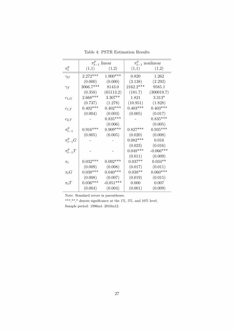
Table 4: PSTR Estimation Results

πpt−1 linear πp

t−1 nonlinearπpt (1,1) (1,2) (1,1) (1,2)

γG 2.272*** 1.900*** 0.820 1.262(0.000) (0.000) (3.138) (2.292)

γT 3066.7*** 8143.0 2162.2*** 9585.1(0.358) (65113.2) (181.7) (300019.7)

c1,G 2.668*** 3.307** 1.821 3.313*(0.737) (1.278) (10.951) (1.828)

c1,T 0.402*** 0.402*** 0.403*** 0.403***(0.004) (0.003) (0.005) (0.017)

c2,T - 0.835*** - 0.835***(0.006) (0.005)

πpt−1 0.916*** 0.909*** 0.827*** 0.935***

(0.005) (0.005) (0.020) (0.008)πpt−1G - - 0.082*** 0.016

(0.023) (0.016)πpt−1T - - 0.048*** -0.066***

(0.011) (0.009)πt 0.032*** 0.092*** 0.037** 0.034**

(0.009) (0.008) (0.017) (0.011)πtG 0.038*** 0.040*** 0.038** 0.060***

(0.008) (0.007) (0.019) (0.015)πtT 0.036*** -0.051*** 0.000 0.007

(0.004) (0.004) (0.001) (0.009)

Note: Standard errors in parentheses.

***,**,* denote significance at the 1%, 5%, and 10% level.

Sample period: 1996m1–2010m12.

27

Table 5: Dynamic Fixed Effects Estimates of Loss Aversion

1996m1–2010m12 1996m1–2007m12πpt (1) (2) (3) (2) (3)

πpt−1 0.935*** 0.938*** 0.940*** 0.957*** 0.964***

(0.007) (0.008) (0.008) (0.008) (0.008)thold1,2 - -0.035 -0.067*** -0.032 -0.061***

(0.022) (0.023) (0.023) (0.023)πt 0.079*** 0.067*** 0.062*** 0.048*** 0.036***

(0.007) (0.010) (0.011) (0.012) (0.013)πt thold1 - 0.021* - 0.020* -

(0.011) (0.012)πt thold2 - - 0.035*** - 0.039***

(0.012) (0.012)constant -0.051** -0.039* -0.037 -0.041 -0.038

(0.022) (0.023) (0.023) (0.028) (0.028)

R2 0.983 0.983 0.984 0.988 0.988AIC -889.848 -894.265 -905.318 -1088.192 -1103.791BIC -878.868 -872.306 -883.358 -1067.130 -1082.730CADF test residuals -5.686 -5.710 -5.664 -5.108 -5.064prob. 0.000 0.000 0.000 0.000 0.000

Note: Correlated panels corrected standard errors in parentheses.

***, **, * denote significance at the 1%, 5% and 10% level, respectively.

28

Figures

Figure 1: Prospect Theory and Inflation Perceptions

29

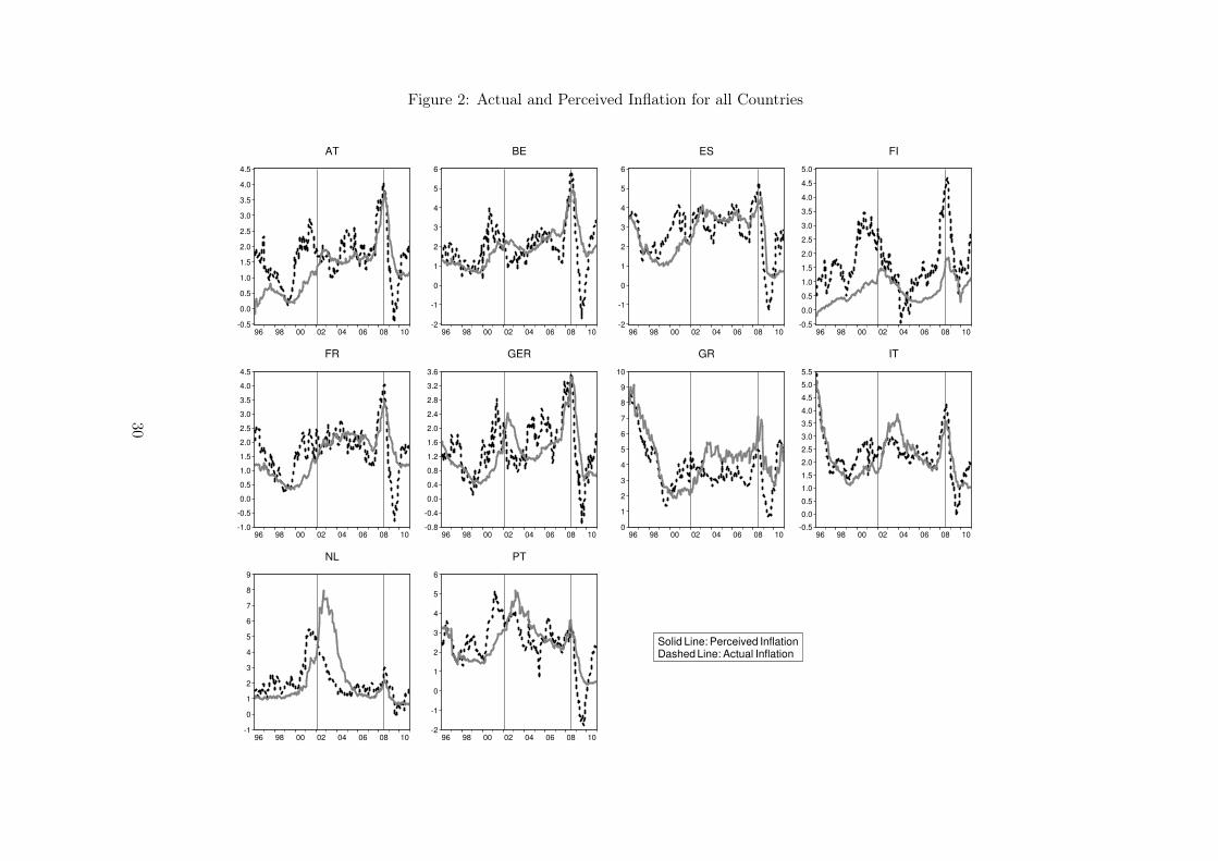
Figure 2: Actual and Perceived Inflation for all Countries

-0.5

0.0

0.5

1.0

1.5

2.0

2.5

3.0

3.5

4.0

4.5

96 98 00 02 04 06 08 10

AT

-2

-1

0

1

2

3

4

5

6

96 98 00 02 04 06 08 10

BE

-2

-1

0

1

2

3

4

5

6

96 98 00 02 04 06 08 10

ES

-0.5

0.0

0.5

1.0

1.5

2.0

2.5

3.0

3.5

4.0

4.5

5.0

96 98 00 02 04 06 08 10

FI

-1.0

-0.5

0.0

0.5

1.0

1.5

2.0

2.5

3.0

3.5

4.0

4.5

96 98 00 02 04 06 08 10

FR

-0.8

-0.4

0.0

0.4

0.8

1.2

1.6

2.0

2.4

2.8

3.2

3.6

96 98 00 02 04 06 08 10

GER

0

1

2

3

4

5

6

7

8

9

10

96 98 00 02 04 06 08 10

GR

-0.5

0.0

0.5

1.0

1.5

2.0

2.5

3.0

3.5

4.0

4.5

5.0

5.5

96 98 00 02 04 06 08 10

IT

-1

0

1

2

3

4

5

6

7

8

9

96 98 00 02 04 06 08 10

NL

-2

-1

0

1

2

3

4

5

6

96 98 00 02 04 06 08 10

PT

Solid Line: Perceived InflationDashed Line: Actual Inflation

30

Figure 3: Inflation vs. Elasticities

.05

.06

.07

.08

.09

.10

.11

.032

.036

.040

.044

.048

.052

.056

-1 0 1 2 3 4 5

AT

.05

.06

.07

.08

.09

.10

.11

.12

.13

.030

.035

.040

.045

.050

.055

.060

.065

.070

-2 -1 0 1 2 3 4 5 6

BE

.068

.072

.076

.080

.084

.088

.092

.096

.100

.104

.108

.025

.030

.035

.040

.045

.050

.055

.060

.065

.070

.075

-2 -1 0 1 2 3 4 5 6

ES

.068

.072

.076

.080

.084

.088

.092

.096

.100

.104

.108

.025

.030

.035

.040

.045

.050

.055

.060

.065

.070

.075

-1 0 1 2 3 4 5

FI

.06

.07

.08

.09

.10

.11

.032

.036

.040

.044

.048

.052

-1 0 1 2 3 4 5

FR

.05

.06

.07

.08

.09

.10

.11

.032

.036

.040

.044

.048

.052

.056

-1 0 1 2 3 4

GER

.068

.072

.076

.080

.084

.088

.092

.096

.100

.104

.108

.025

.030

.035

.040

.045

.050

.055

.060

.065

.070

.075

0 1 2 3 4 5 6 7 8 9

GR

.05

.06

.07

.08

.09

.10

.11

.12

.13

.030

.035

.040

.045

.050

.055

.060

.065

.070

-1 0 1 2 3 4 5 6

IT

.068

.072

.076

.080

.084

.088

.092

.096

.100

.104

.108

.025

.030

.035

.040

.045

.050

.055

.060

.065

.070

.075

-1 0 1 2 3 4 5 6

NL

.068

.072

.076

.080

.084

.088

.092

.096

.100

.104

.108

.025

.030

.035

.040

.045

.050

.055

.060

.065

.070

.075

-2 -1 0 1 2 3 4 5 6

PT

Actual inflation plotted vs. time-varying elasticitiesGray line: pre Euro cash changeoverBlack Line: post Euro cash changeover

31

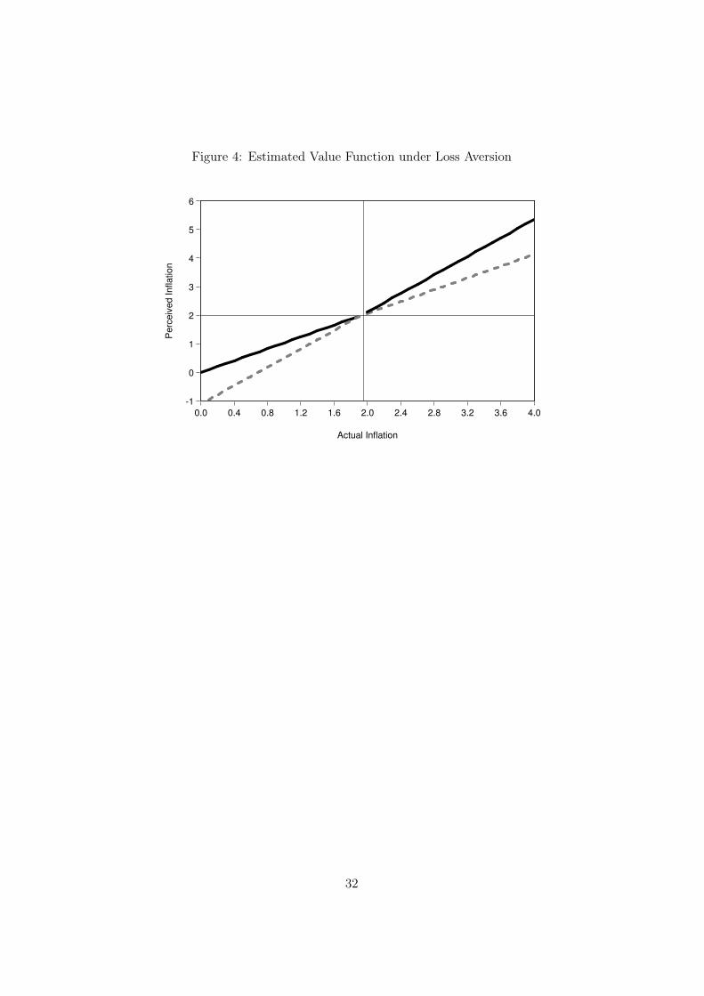
Figure 4: Estimated Value Function under Loss Aversion

-1

0

1

2

3

4

5

6

0.0 0.4 0.8 1.2 1.6 2.0 2.4 2.8 3.2 3.6 4.0

Actual Inflation

Perc

eiv

ed Inflation

32

Appendix

A Quantification technique

Question 5 of the EC Joint Harmonized EU Program of Business and Con-sumer Surveys asks if consumer prices over the past 12 months did:

1. Fall,

2. Stay about the same,

3. Increase at a slower rate,

4. Increase at the same rate,

5. Increase more rapidly.

In an influential paper, Batchelor and Orr (1988) derive how to transformresponses from a pentachotomous survey into a measure of inflation expec-tations/ inflation perceptions. The method is based on and extends theseminal work of Carlson and Parkin (1975).We follow Nielsen (2003) – see Figure 5 below – in the description of themethod and use her terminology. The main assumption underlying such amethod lies in the existence of an interval

(

−δLt , δUt

)

around 0 with δLt , δUt > 0

such that participants in the survey report “no change” in prices (i.e. zero in-flation). Furthermore, there exists another interval

(

µt − εLt , µt + εLt)

aroundthe subjective expected value of the inflation rate µt such that individualsreport that “prices increase at the same rate”.The respective questions of the survey here can be translated into such aconcept in the following way (xt+1 measures the time series of interest –here: “inflation perceptions” which households have to form expectationsabout):27

1. “Fall slightly” if xt+1 ≤ −δLt .

2. “Stay about the same” if −δLt < xt+1 ≤ δUt ,

3. “Increase at a slower rate” if δUt < xt+1 ≤ µt − εLt ,

4. “Increase at the same rate” if µt − εLt < xt+1 < µt + εUt ,

5. “Increase more rapidly” if µt + εUt ≤ xt+1.

27Note that we deal with perceptions as a latent variable which has to be “forecasted” basedon the information set in t. This is in line with models of sticky information as well asmodels of rational inattention where updating of information is costly.

33

We label the fractions of answers in the ordering of the questions fromA to E, respectively, that is: tµt+1 = µt × f (tAt+1, . . . , tEt+1), where

tAt+1, . . . , tEt+1 are the fractions of respondents answering each option, f isa known distribution function (see Batchelor and Orr, 1988, p. 322, formula(11)) and µt is the expected value of the perceived inflation rate that has tobe specified.We use a version of the procedure proposed in Döpke et al. (2008) in orderto determine f and µt: We assume a normal distribution for f and fur-thermore base µt on the medium-term trend of inflation, which householdsare assumed to observe correctly. This is approximated by the HP filter,which is calculated in a recursive way following a quasi-real-time approach.For each period, t, we apply the filter with the usual penalty parameter(λHP = 14400) for monthly data. Finally, we set µt equal to the value ofthe HP filtered inflation as of time t.

Figure 5: Quantification of a Pentachotomous Survey

0-δtL δt

Utµt+1

f(xt+1|Ωt)

xt+1

tAt+1

tBt+1tCt+1

µt

tDt+1

tEt+1

µt-εtL µt+εt

U~ ~ ~

Source: Nielsen, 2003, p.5

34

B Unit Root Tests and Cointegration

Both inflation perceptions and actual inflation rates in our panel are testedfor unit roots over the whole sample period from January 1996 to December2010. We apply five different panel unit root tests: The Levin et al. (2002)test assumes a common unit root process over all series in the sample. Itestimates proxies for ∆yit and yit−1 and tests for the null hypothesis H0 :α = 1 in the regression ∆y∗it = αy∗it−1 + ηit, allowing for individual-specificdeterministic intercepts. However, it suffers from the restriction that nocross-sectional correlation is allowed and that it can only test for stationarityof all series in the sample. By contrast, the tests by Im et al. (2003), Maddalaand Wu (1999) as well as Choi (2001) (Fisher’s ADF and PP test) allow forindividual unit root processes. They specify individual unit root tests andderive test statistics to test the null hypothesis H0 : αi = 0, for all iagainst the alternative that at least one αi 6= 0. While the tests may includeindividual-specific short-run dynamics and deterministics such as time trendsfor each panel member, cross-sectional correlation between countries is stillnot fully accounted for. This may be a relevant issue for actual and perceivedinflation rates in a panel of closely related countries, such as the Europeancountries analyzed here. Therefore, we additionally test for panel unit rootswith the Pesaran (2007) Cross-Sectionally Augmented Dickey-Fuller (CADF)test. The test computes a t-bar statistic averaging t-statistic values forH0 : αi = 0 from a standard ADF-regression augmented with lagged andfirst-differenced values of the cross-sectional mean of the series. All panelunit root tests are calculated with three lags.The test results in Table B.1 uniformly reject the null of a unit root in in-flation in favor of the alternative of stationarity of at least some series inthe panel. However, the null cannot be rejected with the stricter alternativeof stationarity of all series in the Levin et al. (2002) test. Regarding thestationarity of perceived inflation rates in the panel, test results are less con-clusive. The Im et al. (2003) and the Maddala and Wu (1999) tests rejectthe null of a unit root at the 5% level, favoring the alternative of station-arity of some series in the panel. By contrast, the Choi (2001) and, morestrongly, the Pesaran (2007) CADF test cannot reject the null of a unit root.Our results are in line with findings in Lein and Maag (2011), who alsofind that inflation perceptions are more persistent in a similar panel settingfor a shorter sample period. Generally, empirical evidence on the order ofintegration of inflation series is mixed, Altissimo et al. (2006) conclude ina survey that empirical findings seem to lean towards stationarity of inflation.

Due to the inconclusive evidence on stationarity of perceived and actual in-flation in our panel, we furthermore test for panel cointegration betweenperceived and actual inflation. Results are presented for seven panel coin-

35

tegration test statistics proposed by Pedroni (1999, 2001, 2004) that arecalculated by extending the Engle-Granger-framework to the panel settingand testing for stationarity of the residual from a regression with I(1) vari-ables, while allowing for individual fixed effects and time trends. The nullhypothesis of no cointegration (ρi = 1) is tested either against the alternativeof a common cointegrating vector (ρi = ρ < 1) or against the alternative ofindividual cointegrating relationships (ρi < 1). The Kao (1999) panel cointe-gration test is also residual-based, but does not allow for individual-specificdeterministics. Stationarity of the residuals from the first-stage regression isthen tested with a panel ADF test on the null of no cointegration against thealternative of a common cointegrating vector. Finally, the Maddala and Wu(1999) test computes individual Johansen cointegration trace tests and max-imum eigenvalue tests and uses those to obtain a combined Fisher statistic.Gutierrez (2003) conducts a Monte Carlo experiment to compare the powerof Kao (1999) and Pedroni (1999, 2001, 2004) tests and finds that as T getslarge, the Pedroni tests have higher power than the Kao test.Results shown in Table B.2 give strong evidence of a cointegration relationbetween perceived and actual inflation over the whole sample period. AllPedroni tests, as well as the Kao (1999) test, reject the null of no cointegra-tion in favor of the alternative of either a common or individual cointegrat-ing vectors at the 1% level. While the Maddala and Wu (1999) trace testand maximum-eigenvalue test rejects both the null of no and the null of atmost one cointegration relation, test statistics for the latter are significantlysmaller. Our, quite intuitive, result of cointegration between perceived andactual inflation is in line with findings in Lein and Maag (2011) who alsoreport panel cointegration between perceptions and inflation with a slightlydifferent sample.

Table B.1: Panel Unit Root Tests for Perceived and Actual Inflation

Perceptions InflationMethod Stat. Prob.* Stat. Prob.*

Alternative: Stationarity of all series in the panelLevin, Lin & Chu t -1.496 0.067 -0.098 0.461

Alternative: Stationarity of some series in the panelIm, Pesaran and Shin W-stat -2.184 0.015 -4.185 0.000ADF - Fisher Chi-square 33.742 0.028 53.513 0.000PP - Fisher Chi-square 27.530 0.121 66.159 0.000Pesaran CADF t-bar -1.986 0.245 -2.594 0.002

* Probabilities for Fisher tests are computed using an asymptotic Chi-square

distribution. All other tests assume asymptotic normality.

Sample period: 1996m1–2010m12.

36

Table B.2: Panel Cointegration Tests between Perceived and Actual Inflation

Method 1996m1–2010m12

Pedroni Tests (Weighted) Stat. Prob.Alternative hypothesis: common AR coefs.Panel v-Statistic 9.015 0.000Panel rho-Statistic -6.627 0.000Panel PP-Statistic -4.270 0.000Panel ADF-Statistic -3.571 0.000Alternative hypothesis: individual AR coefs.Group rho-Statistic -4.957 0.000Group PP-Statistic -4.058 0.000Group ADF-Statistic -3.270 0.001

Kao ADF Test t-Stat. Prob.-6.154 0.000

Maddala & Wu Test Fisher-Stat.* Prob.Trace test

None 202.600 0.000At most 1 89.980 0.000

Max.-Eigenvalue testNone 165.500 0.000

At most 1 89.980 0.000

* Probabilities for Fisher tests are computed using an asymptotic Chi-square distribution.

Chi-square distribution. All other tests assume asymptotic normality.

37

C Rationality Tests under Symmetric Loss

We applied three types of rationality tests:

• A traditional Mincer-Zarnowitz regression where the perception erroris regressed on a constant and lagged perception errors.

• As a test for bias, we applied the non-parametric test of Dufour (1981)and Campbell and Ghysels (1995) which has the advantage of avoidingrestrictive assumptions on well-behaved residuals as in the case of mostof the regression-based tests. Suppose that we compute the absolutevalue of the difference between each observation and the mean, andthen rank these observations from high to low. Then the test is basedon the idea that the sum of the ranks for the samples above and belowthe median should be similar. We can use a Wilcoxon signed rank testwith the null hypothesis that the median of the perception errors isequal to zero. According to Campbell and Ghysels (1995), this test ispreferable to parametric tests for small samples.

• As a test for efficiency, we again use a test proposed by Dufour (1981)and Campbell and Ghysels (1995) to test for absence of serial correla-tion in the forecasts errors, i. e. that the median of the product of twoconsecutive perception errors is centered on a median of zero.

We do not report the Mincer-Zarnowitz results here as the result is well-known from other studies, see for instance Jonung and Laidler (1988), Leinand Maag (2011) and Dräger (2011). Rationality under symmetric loss isrejected in all cases, irrespective of controlling for possible structural breaksat the end of 2001 or 2007. The results, however, are available from theauthors upon request.This rejection is probably to a large extent driven by the “inefficiency chan-nel”. The results of the two non-parametric tests shown in table (C.1) re-vealed that in a number of cases we cannot reject unbiasedness once wecontrol for possible structural breaks by splitting the sample appropriately.However, efficiency is rejected in all cases irrespective of sample splits.

38

Table C.1: Nonparametric Rationality Tests: Unbiasedness and Efficiency

Unbiasedness

1996m1–2010m12 1996m1–2001m12 2002m1–2010m12 1996m1–2007m12Country Stat. Prob. Stat. Prob. Stat. Prob. Stat. Prob.

AT 6.840 *** 7.287 *** 1.884 * 8.040 ***BE 0.921 6.114 *** 3.321 *** 1.892 *ES 3.585 *** 6.602 *** 0.887 3.924 ***FI 10.827 *** 7.371 *** 7.557 *** 9.542 ***FR 3.522 *** 6.467 *** 1.053 4.231 ***GER 3.219 *** 4.756 *** 0.379 4.492 ***GR 6.153 *** 1.086 6.533 *** 5.362 ***IT 2.098 ** 4.823 *** 1.203 1.987 **NL 2.746 *** 7.354 *** 2.224 ** 1.638PT 0.542 5.530 *** 3.664 *** 1.630

Efficiency

1996m1–2010m12 1996m1–2001m12 2002m1–2010m12 1996m1–2007m12Country Stat. Prob. Stat. Prob. Stat. Prob. Stat. Prob.

AT 10.608 *** 7.165 *** 7.554 *** 9.499 ***BE 10.153 *** 6.185 *** 8.095 *** 8.993 ***ES 10.690 *** 6.902 *** 8.089 *** 9.450 ***FI 11.418 *** 7.320 *** 8.589 *** 10.222 ***FR 9.944 *** 6.804 *** 7.277 *** 8.304 ***GER 10.569 *** 6.627 *** 8.225 *** 9.557 ***GR 11.307 *** 6.907 *** 8.887 *** 10.081 ***IT 10.823 *** 6.844 *** 8.284 *** 9.573 ***NL 11.240 *** 7.251 *** 8.524 *** 10.236 ***PT 10.478 *** 6.294 *** 8.381 *** 9.353 ***

Test statistic: Wilcoxon signed rank.

***, **, * denote significance at the 1%, 5% and 10% level, respectively.

39

D Structural Break Tests

Table D.1: Quandt-Likelihood-Ratio Test for Structural Breaks

Country Lossaversion with thold1 Lossaversion with thold2Max. Wald F p-value date Max. Wald F p-value date

AT 53.892 0.000 2008m09 53.008 0.000 2008m09BE 30.449 0.000 2008m06 33.299 0.000 2008m06ES 16.170* 0.055 2003m07 25.271* 0.002 2006m06FI 23.190 0.008 2008m04 24.821 0.004 2007m12FR 30.074 0.000 2002m02 37.286 0.000 2008m03GER 42.598 0.000 2007m08 41.840 0.000 2007m09GR 23.495 0.007 2008m07 18.962** 0.011 2002m09IT 22.528 0.010 2008m07 23.272 0.007 2008m07NL 25.205 0.003 2002m10 36.786 0.000 2002m10PT 13.157 0.247 1998m06 9.152* 0.451 2001m06

Note: *, ** denotes 30%, 40% trimmed data, respectively. The default is 15% trimmed data.

Sample period: 1996m1–2010m12.

40