Pension Reform and Savings

Page 1

Pension Reform and Savings

Emma Aguila�

University College London (UCL)y

April 2005

Abstract

Latin American pension reforms from a pay-as-you-go to a fully funded system withindividual accounts have been encouraged by policymakers under the premise that theypromote private savings. However, this research provides evidence from the Mexican pensionreform which could contradict that assumption.

The main results of this analysis show that the pension reform increased consumptionand crowded out savings of low income workers, who are the majority of population a¤ectedby the reform. These �ndings are consistent with the Life Cycle model predictions asthe theoretical analysis shows that the pension reform caused an income and a pensionwealth e¤ect particularly for low income employees. The empirical evaluation is conductedusing a nonparametric di¤erence-in-di¤erences estimator implemented with propensity scorematching.

JEL classi�cation: D91, H55, J26Keywords : Pension reform; Household savings; Mexico

1. Introduction

In Latin American countries such as Chile, Argentina, Colombia, Bolivia, and Mexico, among

others, pension reforms from a pay-as-you-go (PAYG) to a fully funded system with individual

accounts were encouraged by policymakers and leading experts in the �eld as having the ad-

vantage of increasing private savings.1 To date, research only provides macro evidence of the

overall impact of Latin American pension reforms on private savings. Studies have exclusively

considered the amount of pension funds accumulated in the individual retirement accounts (IRA)

and the negative e¤ect of the reform�s �scal cost.2

This literature has not explored the impact of changes in pension wealth as a result of the

pension reform and its e¤ects on households�decision for holding other assets.3 It is fundamental

to assess the crowding out e¤ects of the pension reform on other types of household assets because

�Acknowledgements: I am grateful for the advice and support of Costas Meghir. I also wish to thank OrazioAttanasio, James Banks, Erich Battistin and Marcos Vera-Hernandez for their valuable comments. Finally, Iwould like to thank CONACYT for the �nancial support.

yEconomics Department, University College London, Gower Street, London, WC1E 6BT, UK. Tel: 020 76 7958 91. E-mail: [email protected].

1For a review on the proposals that this type of pension reform boosts savings see Orszag and Stiglitz (1999).Moreover, for a description of pension reforms in Latin American countries see Mesa-Lago (2001).

2A survey on the impact of the pension reform on savings for Latin American countries is presented in Mesa-Lago (2004). For the Mexican case see Sales et al. (1996) and Solís and Villagómez (1999).

3 In the most recent evaluation of Latin American pension reforms presented in Gill et al. (2004), this issueremains aside of the main stream of analysis.

1

Page 2

they could o¤set the boost in savings caused by the transfer of opaque pension funds to a more

e¢ cient management in the �nancial market. The scope of this paper is to examine this issue

by using evidence from the Mexican case.

In economic theory, consumption and savings decisions are generally analyzed using Modigliani

and Brumberg�s Life Cycle Hypothesis. The simplest version of the model states that individu-

als save during working life and dissave in old age. Related literature tests the Life Cycle model

predictions empirically, investigating whether increases in pension wealth crowd out households�

savings. Feldstein�s seminal paper (1974) provides empirical evidence that social security wealth

decreases personal saving by 30 to 50 percent.

The most recent studies that examine household behavior are Attanasio and Brugiavini (2003)

and Attanasio and Rohwedder (2003). Both �nd evidence consistent with the Life Cycle Model.

Attanasio and Rohwedder show that the elasticity of substitution between pension wealth and

�nancial wealth increases with age in the UK. As the individual approaches retirement age,

pension wealth is a better substitute for �nancial wealth. Attanasio and Brugiavini suggest that,

as a result of the 1992 Italian pension reform, a decrease in pension wealth caused an increase

in savings.

However, there are other studies that report no e¤ect, such as Euwals (2000) and Gustman

and Steinmeier (1998). Euwals concludes that mandatory pensions have no impact on household

savings in the Netherlands. Gustman and Steinmeier using U.S. data from the Health and

Retirement Study (HRS) �nd that pensions have a very limited e¤ect on displacing any other

kind of wealth.

In this study, the e¤ects of the Mexican pension reform on households consumption and

savings are analyzed within the framework of the Life Cycle model. In Mexico, a pension reform

was implemented in 1997 with the major goals of increasing private savings and securing a

�nancially feasible pension scheme. The public pension plan with the highest coverage, mainly

mandatory for private sector workers, changed from a PAYG to IRA. It was an extreme pension

reform that changed the public unfunded de�ned bene�t system to a private funded de�ned

contribution plan.4 The pension reform was a response to a growing concern about the low

levels of private savings and an unsustainable �nancial imbalance of public pension schemes.

This pension reform a¤ected 38% of the labor force and 50.6% of the formal sector.

Furthermore, the study of the Mexican case is pertinent because it allows testing the e¤ects

4The most moderate type of pension reforms are parametric, where a combination of features such as retirementage, contributions or bene�ts are modi�ed, maintaining the public or private provision. See Lindbeck and Persson(2003) for classi�cations of pension reforms.

2

Page 3

of the most radical type of pension reform. Also, the impact of the pension reform is naturally

isolated from substitution of alternative sources of pension wealth as most of Mexican households,

in contrast to the US and UK, do not have other type of annuitized income during retirement

such as occupational and personal pensions.

This study is organized as follows. The next section describes key changes of the Mexican

pension reform. The third section presents the theoretical framework, the income and pension

wealth e¤ects of the pension reform, and the main predictions of the Life Cycle model. The

fourth section describes the evaluation methodology and the data used. The �fth section shows

the estimation procedures and results. Finally, this research presents a brief conclusion and o¤ers

some policy recommendations.

The empirical impact of the pension reform is estimated using a nonparametric di¤erence-

in-di¤erences estimator obtained with propensity score matching. The data set is from the

Mexican National Survey of Household Income and Expenditure. It has detailed information on

consumption and income. It also allows the identi�cation of a comparison group, which is used

to evaluate the pension reform as an experiment.

The main �ndings of this analysis are that low income workers, particularly those earning

below �ve times the minimum wage, increase their consumption and decrease savings. There is

no e¤ect for workers earning more than �ve times the minimum wage. These results are in line

with the predictions of the Life Cycle model given the features of the Mexican pension reform.

2. Mexican Pension System

The public pension scheme with the highest coverage is managed by the Mexican Social

Security Institute (IMSS), founded in 1943. This institute o¤ers healthcare services, nurseries,

recreational centers, bene�ts for disability, compensation for work injuries, and a pension plan. At

the end of the 1980�s, the PAYG pension plan had a �nancial imbalance caused by an increasing

proportion of retirees with respect to the number of workers contributing to the system and

continuous changes to pension wealth without adjusting contribution rates. In addition, the

pension system had no reserves because annual surpluses were transferred to other services,

mainly healthcare.

In 1992 a pension reform introduced complementary individual retirement accounts managed

by the Central Bank (SAR). The balance of SAR individual account was given to the worker at

retirement as a one-o¤ payment in addition to the PAYG pension. Therefore, the 1992 reform

3

Page 4

only increased pension wealth at retirement, diminishing income e¤ects induced by the transition

from employment to retirement status. More importantly, this reform did not reduce the �nancial

de�cit of the PAYG system (section A.1 of Appendix A presents a more detailed description of

the reform). Furthermore, SAR had many management ine¢ ciencies and the PAYG had an

unsustainable de�cit that led to the approval of a major pension reform in December 1995.

The reform approved in December 1995 determined the substitution of the PAYG scheme for

IRA from the 1st of July 1997. The IRA are individual savings accounts for retirement managed

by private retirement fund managers (AFORES). Thus, from the 1st of July 1997, all workers,

new and transition generation started contributing to the IRA.

The transition generation group includes employees that contributed to the PAYG system. In

order to recognize their previous contributions to the PAYG, this group has the option to choose

at retirement the highest pension under the former and current rules. It is worth mentioning

that while the transition generation retires, the PAYG scheme still has a �nancial imbalance,

which is gradually covered by the government. Thus, the �scal cost of the Mexican pension reform

depends on the transition generation individuals retiring under the PAYG rules and those retired

before the reform was enforced. The main features of the PAYG and IRA schemes are described

below.

2.1. Pension Requirements

Under the PAYG and IRA schemes, it is necessary to satisfy the retirement age and a

minimum of contribution years to obtain a pension. The normal retirement age is 65 years old

and early retirement is from age 60 under the PAYG and IRA rules. The PAYG requires only

10 years of contribution but this changed to 25 years under the IRA.

Services provided by IMSS are �nanced with a monthly payroll tax levied to employer, em-

ployee and government. The reform only changed government contributions to the pension

scheme by US$5 per month as a result of the introduction of a �at rate called social quota. Em-

ployer and employee contributions represent 10.075% of employee�s wage. Only 2.125% is covered

by the worker and the rest by the employer. However, the reform changed completely contri-

butions to healthcare services provided by IMSS. A detailed description of IMSS�s contributions

scheme is presented in section A.2.1. of Appendix A.

2.2. Pension Bene�ts

The procedure to compute the PAYG and IRA pension is as follows. The PAYG pension

4

Page 5

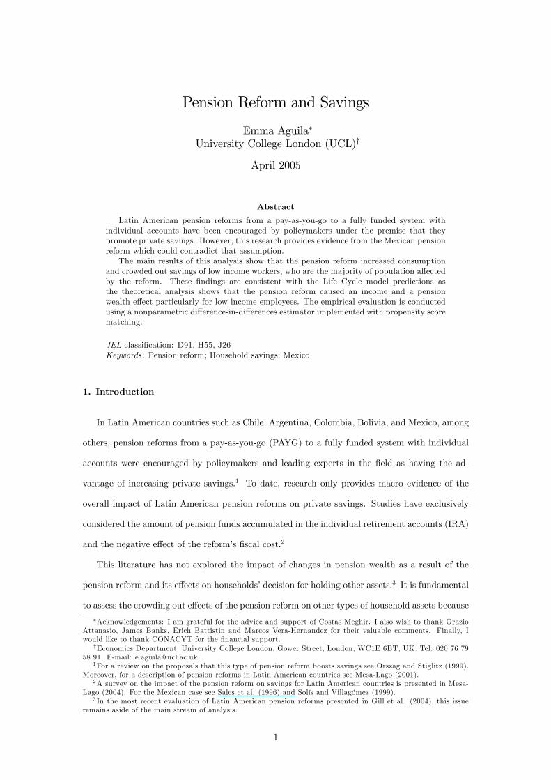
is a proportion of the average wage of the previous �ve years to retirement plus a fraction for each

year that the worker contributed above the minimum requirement. This bene�t scheme is similar

to a �nal salary de�ned bene�t plan. The replacement rate is a decreasing function of�w, which

is the ratio of the average wage of the previous �ve years to retirement by the minimum wage,

as shown in Fig.1 (a).5 Therefore, the scheme�s progressive rule assigns low income employees a

high replacement rate, and to higher income employees a low replacement rate.

010

203040

506070

8090

1 2 3 4 5 6 7 8 9 10 11 12 13 14 15

repl

acem

ent r

ate

(%)

0.4

0.6

0.8

1

1.2

1.4

1.6

1.8

2

2.2

1 2 3 4 5 6 7 8 9 10 11 12 13 14 150

5

10

15

20

25

mon

thly

pen

sion

workers affiliated to IM

SS (%)

(a) (b)

0.50.70.91.11.31.51.71.92.12.32.5

1 2 3 4 5 6 7 8 9 10 11 12 13 14 15

repl

acem

ent r

ate

(%)

0

10

20

30

40

50

60

70

80

90

100

1 2 3 4 5 6 7 8 9 10 11 12 13 14 15

repl

acem

ent r

ate

(%)

40 years of contribution

20 years of contribution

10 years of contribution

(c) (d)Fig. 1. Replacement rates and monthly pension. (a) minimum years of contribution.

(b) normal retirement. (c) additional years of contribution. (d) 10, 20 or 40 years of contribution.

The bold line in Fig.1 (b), shows the monthly PAYG pension for each level of�w. Individuals

with�w below seven obtain the minimum wage as shown by the dotted line, which is the minimum

pension. The solid line indicates the earnings distribution of workers enrolled to IMSS and it is

measured in the axis to right.

It is worth highlighting that most of workers earn between two and four times the minimum

wage. Thus, the distribution of pensions is skewed towards the minimum wage. For example,

a median worker who has a monthly labor income (�w) of 3.7 times the minimum wage, the

replacement rate is 22.07%, and the monthly PAYG pension is equivalent to 0.94 times the

minimum wage, although she receives a minimum pension.6

In addition, employees obtain a compensation for every year of contribution above the mini-

mum requirement. Fig.1 (c) shows the replacement rate for the additional years of contribution,

5For consistency with IMSS�s regulation, the ratio w is interpreted as the average wage in number of times theminimum wage. For example, w = 2 implies that the individual earns twice the monthly minimum wage.

6Workers receive an additional increment in their pension when they qualify for family bene�ts such as wid-owhood and number of children under 16 years old, among others. The monthly pension estimations in �gure1(b) and 1(d) include the minimum increment for family bene�ts provided by IMSS.

5

Page 6

which is an increasing function of�w. This e¤ect is illustrated in Fig.1 (d). A low income in-

dividuals with�w = 1 obtain the minimum pension which is the minimum wage of Mexico City

after contributing for 10, 20 or 40 years. In contrast, higher income individuals with�w = 12 are

eligible to a monthly pension of 1.56 times the minimum wage after contributing for 10 years, 4.5

times the minimum wage with 20 years and after 40 years, 10.38 times the minimum wage. Con-

sequently, low income workers have fewer incentives to contribute for more than 10 years. Higher

income individuals have incentives to contribute more than the minimum required because they

receive only 13% of�w having completed 10 years of contribution, but 87% for 40 years. In the

latter, the PAYG scheme is more generous than a de�ned contribution according to the actuarial

saving rule 60:40:20:10:5:2.7

The contribution incentives of the PAYG are consistent with the empirical evidence. Low

income workers have higher rotation rates and migration to the informal sector. Higher income

workers tend to have more stable jobs and few unemployment spells, so they are able to contribute

throughout their working life.

Furthermore, the PAYG pension could be received before age 65 with a reduction of 5% for

each year to a maximum of 25% when retiring at age 60. The penalty to retire below the normal

retirement age is actuarial equivalent as the present value of the early retirement pensions is equal

to the pension at age 65. Workers whose normal retirement pension is the minimum guarantee as

a result that their pension is below the minimum wage have incentives to choose early retirement

because they do not su¤er any reduction. Otherwise, workers with a pension higher than the

minimum guarantee would prefer to reach normal retirement age as the pension rises 5% plus

the increment for each year of contribution above the requirement of 10 years.

After age 65, the pension only increases with the additional years of contribution and there

is not limit of age to retire. There are more incentives to continue contributing after age 65 for

higher labor income workers as the replacement rate for additional years of contribution rises

with wage. The increment in the pension after age 65 for low income workers is not actuarially

fair because the contribution of every additional year is higher than the increase in the present

value of the pension.

The IRA pension is computed dividing the balance of the individual account by the average life

expectancy at retirement. The employee can choose between an annuity provided by a private

7The actuarial saving rule 60:40:20:10:5:2 implies that in a de�ned contribution scheme an individual obtainsa pension equivalent to 60% of the salary after contributing for 40 years assuming a life expectancy at retirementof 20 years, a 10% contribution rate, 5% rate of return, and 2% earnings growth.

6

Page 7

insurance company or programmed withdrawals from the retirement fund manager AFORE.

The IRA pension depends on the interest rate performance and the amount deposited. This is a

characteristic of de�ned contribution schemes, which are closely linked to contributions.

An enhanced feature of the scheme is that pensions are adjusted to in�ation instead of

the minimum wage of Mexico City. It is worth highlighting that historically, minimum wage

improvements have been lower than increase in prices. The real minimum wage has su¤ered a

depreciation of 6.4% per year on average over the last decade. Therefore, the PAYG pension

depreciates at a higher rate than the IRA due to the in�ationary loss. Finally, the IRA�s minimum

pension guarantee is also the minimum wage of Mexico City.

2.3. Fiscal Incentives and Voluntary Savings

The 1997 reform introduce a less favorable �scal structure, imposing a tax to IRA�s

earnings. In contrast to the earnings of the 1992 individual account which were exempt. The

�scal scheme for contributions and pension wealth did not change. Contributions are taxed and

pension wealth exempt.

Furthermore, the pension reform launched the possibility of voluntary savings to the IRA.

The advantages are: a) voluntary savings are managed separately from mandatory contributions,

b) employer and employee contributions are deductible, and c) employees can withdraw funds

every 6 months. However, monthly contributions should not exceed 2% of worker�s wage, and

earnings and funds withdrawn before retirement are taxed.

Subsequently, in 1999 some of these features were modi�ed. IRA�s earnings and funds with-

drawn before retirement are not taxed, but employer contributions are not deductible any more.

Hence, IRA�s voluntary saving component has not been intended to target any speci�c group of

savers and it is not especially attractive.

For a worker earning the minimum wage, the transaction costs of saving the maximum

monthly limit are higher than the amount saved. The regulatory framework does not encourage

low income workers to save in the voluntary option of the IRA. In comparison, the U.S. retire-

ment savings accounts (IRAs and 401k) have a limit to annual contribution, which gives more

incentives to middle and low income workers to save.

These arguments could explain the low levels of voluntary saving, which represented 0.56% of

mandatory contributions in December 2003. It is likely these savings were just reallocated from

other type of assets. It would be interesting for further research to evaluate the e¤ectiveness of

7

Page 8

the voluntary scheme to generate new saving.

3. Theoretical Framework

According to the Life Cycle Hypothesis (LCH), individuals maximize consumption during

their life span in order to smooth the marginal utility of consumption across periods. Consump-

tion and saving behavior are analyzed within a simple version of the Life Cycle Model with three

periods. During the �rst two periods the individual is in the labor market, and in the third

period retires. A three period model is applied to examine the e¤ects of the reform for the new

and transition generations.

The LCH predicts a degree of substitutability between pension wealth and household assets.

Pension wealth may not be a perfect substitute of other type of saving because pensions are not

liquid assets. In the model, disposable income is allocated between consumption and savings.

Assume the utility function is iso-elastic and intertemporally separable:

U(C1; C2; C3) =3Xt=1

�t�1C1��t

1� � (1)

The utility function depends on consumption in every period Ct. The consumption elasticity

of substitution is 1� , and � is the discount factor. The budget constraint speci�es that the present

value of lifetime consumption is lower or equal than the present value of net labor income (W )

and a pension (P ):83Xt=1

Ct(1 + r)t�1

�2Xt=1

Wt

(1 + r)t�1+

P

(1 + r)2(2)

where, r is the interest rate. Another assumption is that there are no bequests. Thus,

the individual does not have assets in period 1, and all wealth is consumed by the last period.

Borrowing or lending is possible, but at the end of the life span there must be no debt. Savings are

de�ned as St = (1+r)St�1+Wt�Ct. Consumption in the third period is C3 = (1+r)S2+P: The

maximization of the utility function subject to the budget constraint gives the optimal conditions

for consumption in every period:

C1 =1

m

�W1 +

W2

(1 + r)+

P

(1 + r)2

�(3)

C2 =�1� (1 + r)

1�

m

�W1 +

W2

(1 + r)+

P

(1 + r)2

�(4)

C3 =�2� (1 + r)

2�

m

�W1 +

W2

(1 + r)+

P

(1 + r)2

�(5)

8Net labour income is income after discounting income tax and social security contributions.

8

Page 9

where, m = 1 + �1� (1 + r)

1��� + �

2� (1 + r)

2�2�� . Savings in every period are obtained by

substituting the value of Ct. Thus, in this model consumption and savings are jointly determined.

According to the optimal conditions, a rise in P increases consumption and decreases savings

through working life. A rise in W increases consumption and savings. The increase in savings

depends on the marginal propensity to save. The pension reform potentially a¤ects labor income

and pension wealth of new and transition generation workers.

The new generation are those individuals that when the reform was implemented were outside

the formal labor market. On the contrary, the transition generation was already in the formal

labor market, in the �rst or second period of their working life. The latter reoptimize their

consumption and saving choices with the new values of net labor income and pension wealth

induced by the pension reform.

The impact on consumption and savings is higher for the transition generation because they

allocate the e¤ect in a shorter length of time. The following section analyses the e¤ects of the

pension reform on labor income and pension wealth for the new and transition generations.

3.1. Income E¤ects of the Reform

The pension reform a¤ected workers�labor income due to the decrease in IMSS�s health-

care services contributions as there were no changes to the pension scheme. Fig. 2 illustrates the

increase in worker�s wage as a result of the pension reform. For consistency with the previous

section, labor income is interpreted as the ratio of the worker wage to the minimum wage.

0.00.51.01.52.02.53.03.54.04.55.0

1 2 3 4 5 6 7 8 9 10 11 12 13 14 15 16 17 18 19 20 21 22 23 24 25 26 27 28monthly labor income

%

Fig. 2. Increase in worker�s labor income as a result of the pension reform.

There is no e¤ect on workers earning the minimum wage because the Labour Law establishes

that in those cases employers pay all contributions. However, workers earning more than the

9

Page 10

minimum wage have an income e¤ect. The highest bene�t is for workers earning less than three

times the minimum wage with an increase in their monthly labor income of 2.87%. For higher

income individuals the change is smaller.

3.2. Pension Wealth E¤ects of the Reform

Pension wealth e¤ects have di¤erent sources for the new and transition generations. The

new generation is compared to the non-reform and reform scenarios. In the non-reform scenario

it is assumed that the PAYG system is still valid for generations entering the labor market after

1997.

For the transition generation the PAYG and IRA pensions are computed to compare which

one they would choose at retirement. In both cases the present value of the pensions at retirement

are computed as follows:

PV PPAY G =IX

i=R

PPAY G � (1� �)i�R+1(1 + �)i�R

(6)

PV P IRA =IX

i=R

P IRA

(1 + �)i�R(7)

PV P is the present value of the PAYG or IRA pension, I is the total life span, � is the annual

in�ationary loss (� > 0), and � is the discount rate.9 As the IRA is indexed to in�ation, � = 0.

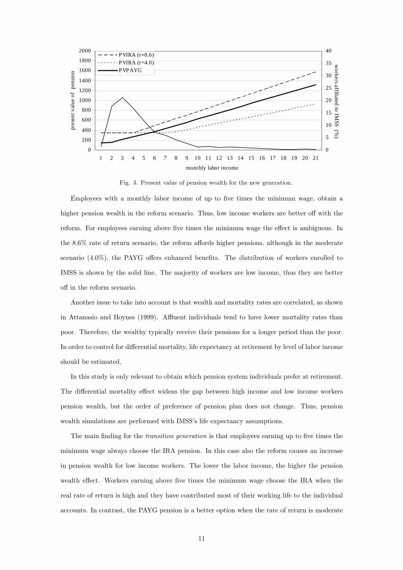
Fig. 3 shows the results of the simulations for men of the new generation. Those for women

are very similar because the rules to obtain a pension are the same, only the life expectancy

is di¤erent. Women receive the pension for a longer period of time obtaining a higher pension

wealth but the order of preferences with respect to the type of pension scheme is not altered.

The IRA pensions were estimated using two real interest rate scenarios: an optimistic 8.6%

and a more conservative 4.0%. The optimistic scenario is a historic average of the IRA real

rate of return. The simulations assumptions are described in more detail in section A.2.2. of

Appendix A.

9The net present value (NPV) of pension wealth is not computed because the total amount of contributionsduring their working life is the same for the PAYG and IRA as contributions to the pension scheme did notchange.

10

Page 11

0

200

400

600

800

1000

1200

1400

1600

1800

2000

1 2 3 4 5 6 7 8 9 10 11 12 13 14 15 16 17 18 19 20 210

5

10

15

20

25

30

35

40PVIRA (r=8.6)PVIRA (r=4.0)PVPAYG

monthly labor income

workers affiliated to IM

SS (%)

pres

ent v

alue

of

pens

ion

Fig. 3. Present value of pension wealth for the new generation.

Employees with a monthly labor income of up to �ve times the minimum wage, obtain a

higher pension wealth in the reform scenario. Thus, low income workers are better o¤ with the

reform. For employees earning above �ve times the minimum wage the e¤ect is ambiguous. In

the 8.6% rate of return scenario, the reform a¤ords higher pensions, although in the moderate

scenario (4.0%), the PAYG o¤ers enhanced bene�ts. The distribution of workers enrolled to

IMSS is shown by the solid line. The majority of workers are low income, thus they are better

o¤ in the reform scenario.

Another issue to take into account is that wealth and mortality rates are correlated, as shown

in Attanasio and Hoynes (1999). A­ uent individuals tend to have lower mortality rates than

poor. Therefore, the wealthy typically receive their pensions for a longer period than the poor.

In order to control for di¤erential mortality, life expectancy at retirement by level of labor income

should be estimated.

In this study is only relevant to obtain which pension system individuals prefer at retirement.

The di¤erential mortality e¤ect widens the gap between high income and low income workers

pension wealth, but the order of preference of pension plan does not change. Thus, pension

wealth simulations are performed with IMSS�s life expectancy assumptions.

The main �nding for the transition generation is that employees earning up to �ve times the

minimum wage always choose the IRA pension. In this case also the reform causes an increase

in pension wealth for low income workers. The lower the labor income, the higher the pension

wealth e¤ect. Workers earning above �ve times the minimum wage choose the IRA when the

real rate of return is high and they have contributed most of their working life to the individual

accounts. In contrast, the PAYG pension is a better option when the rate of return is moderate

11

Page 12

or they have contributed fewer years to the IRA. Hence, the e¤ect for higher income workers is

ambiguous, depending on their expectations of the rate of return and the years of contribution

to the IRA.

Individuals that do not continue to contribute for up to 25 years satisfying the IRA require-

ments, can only retire under the PAYG rules. The transition generation simulations are done

for di¤erent combinations of IRA and PAYG contribution years. A summary of the results is

presented in Table A.4. of Appendix A.

3.3. Predictions of the Life Cycle Model

In sum, the pension reform caused an income and pension wealth e¤ect for low income

workers. For high income individuals the pension wealth e¤ect is ambiguous and the increase

in income is small. The rise in pension wealth for low income individuals is explained by their

eligibility to a minimum pension that depreciates at a lower rate under the IRA.10 For higher

income workers the PAYG is more generous in comparison to the IRA under a moderate rate of

return scenario.

The predictions of the Life Cycle Model are an increase in consumption and a decrease in

savings for low income individuals due to the rise in their pension wealth. The income e¤ect

causes an additional increase in consumption and a rise in savings. As a consequence of the

income e¤ect, part of the former decrease in savings is compensated. Its extent depends on

the marginal propensity to save. Higher income individuals slightly increase consumption and

savings because of a rise in their labor income by around 1.2%.

Furthermore, the reform potentially changed the credibility of the pension system. When

individuals perceive an uncertain pension system, they may react by increasing precautionary

savings. Policymakers have argued that the IRA could induce more credibility in the pension

scheme. The main reasons are the following.

First, workers can monitor pension savings through regular AFORE�s statements. Second,

accrued funds can be withdrawn when the worker stops contributing to the scheme. These bene�t

workers with high labor turnover and individuals that tend to have long periods out of the labor

market. Finally, the voluntary savings option gives low income earners access to the �nancial

market. Thus, it may be expected that individuals recognize a more certain pension system and

decrease their precautionary savings. These arguments are oriented to induce more certainty

10 In 2001, PAYG pensions were modi�ed to be in�ation adjusted, increasing pension wealth for individualsretired before the 1997 pension reform.

12

Page 13

particularly to low income workers given their high rotation rates and probability to spend part

of working life in the informal sector.

The following sections present the empirical results of the e¤ects of the 1997 pension reform

only for the transition generation. As the available data are repeated cross-sections, it is not

possible to identify individuals from the new generation before the reform, when they were

outside the formal labor market.

4. Empirical Methodology

The e¤ects of the 1997 pension reform are evaluated with a di¤erence-in-di¤erences

estimator obtained with propensity score matching (Heckman et al., 1997). Matching mim-

ics experimental methods using non-experimental data. The matching method is implemented

nonparametrically with a Kernel function. The estimations using Nearest Neighbor and linear

matching are also presented to analyze the robustness of the results.

In a previous study, Attanasio and Rohwedder (2003) empirical methodology is a structural

model that tests the e¤ects of the variation in pension wealth as a result of UK pension reforms

during the 1970�s and 1980�s. The data set are cross-sections from the Family Expenditure Sur-

vey (FES). In Attanasio and Brugiavini (2003) empirical methods are a di¤erence-in-di¤erences

estimator implemented with regression discontinuity design. The data are repeated cross-sections

of one year before and one year after the 1992�s Italian pension reform.

In this research, matching methods in comparison to other program evaluation estimators,

is appropriate because the pension reform a¤ects all individuals contributing to IMSS. More-

over, the data available are repeated cross-sections which provide a unique source to identify a

comparison or control group.

4.1. Evaluation Methods

The impact on consumption and savings is obtained by comparing outcomes in the case of

being a¤ected by the pension reform or treatment and in the case of not receiving the treatment.

As the data are cross-sections, workers are identi�ed before and after the pension reform.

Let Cit denote the outcome in treatment status i and period t. A person in state i = 1 is a

treated unit who transferred from the PAYG to the IRA as a result of the pension reform. A

person in state i = 0 is a non-treated or control unit that contributed to the PAYG before and

after the pension reform.

13

Page 14

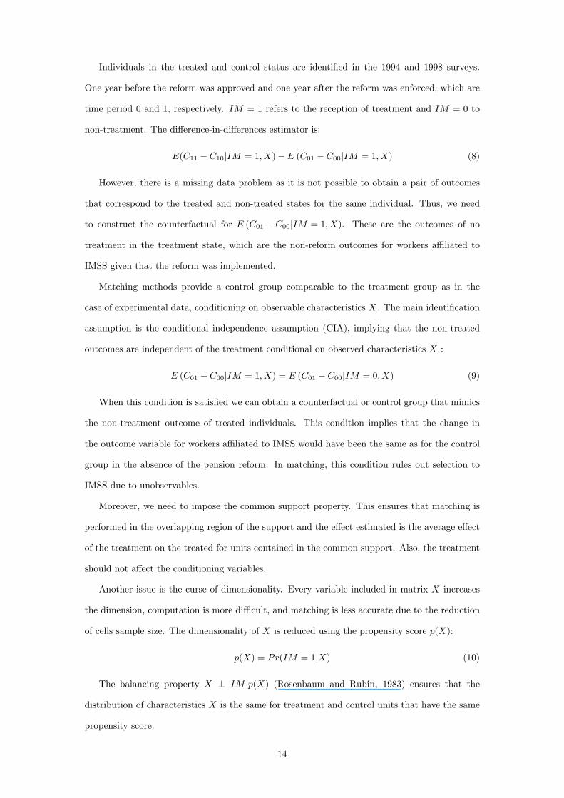
Individuals in the treated and control status are identi�ed in the 1994 and 1998 surveys.

One year before the reform was approved and one year after the reform was enforced, which are

time period 0 and 1, respectively. IM = 1 refers to the reception of treatment and IM = 0 to

non-treatment. The di¤erence-in-di¤erences estimator is:

E(C11 � C10jIM = 1; X)� E (C01 � C00jIM = 1; X) (8)

However, there is a missing data problem as it is not possible to obtain a pair of outcomes

that correspond to the treated and non-treated states for the same individual. Thus, we need

to construct the counterfactual for E (C01 � C00jIM = 1; X). These are the outcomes of no

treatment in the treatment state, which are the non-reform outcomes for workers a¢ liated to

IMSS given that the reform was implemented.

Matching methods provide a control group comparable to the treatment group as in the

case of experimental data, conditioning on observable characteristics X. The main identi�cation

assumption is the conditional independence assumption (CIA), implying that the non-treated

outcomes are independent of the treatment conditional on observed characteristics X :

E (C01 � C00jIM = 1; X) = E (C01 � C00jIM = 0; X) (9)

When this condition is satis�ed we can obtain a counterfactual or control group that mimics

the non-treatment outcome of treated individuals. This condition implies that the change in

the outcome variable for workers a¢ liated to IMSS would have been the same as for the control

group in the absence of the pension reform. In matching, this condition rules out selection to

IMSS due to unobservables.

Moreover, we need to impose the common support property. This ensures that matching is

performed in the overlapping region of the support and the e¤ect estimated is the average e¤ect

of the treatment on the treated for units contained in the common support. Also, the treatment

should not a¤ect the conditioning variables.

Another issue is the curse of dimensionality. Every variable included in matrix X increases

the dimension, computation is more di¢ cult, and matching is less accurate due to the reduction

of cells sample size. The dimensionality of X is reduced using the propensity score p(X):

p(X) = Pr(IM = 1jX) (10)

The balancing property X ? IM jp(X) (Rosenbaum and Rubin, 1983) ensures that the

distribution of characteristics X is the same for treatment and control units that have the same

propensity score.

14

Page 15

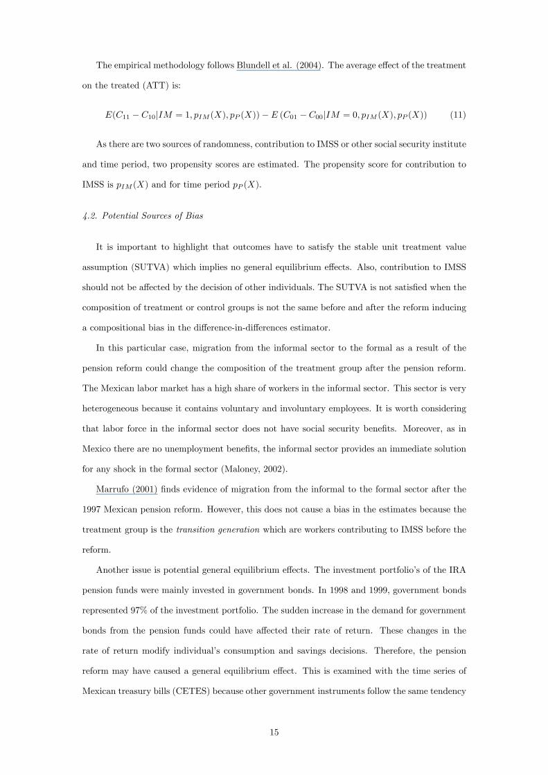
The empirical methodology follows Blundell et al. (2004). The average e¤ect of the treatment

on the treated (ATT) is:

E(C11 � C10jIM = 1; pIM (X); pP (X))� E (C01 � C00jIM = 0; pIM (X); pP (X)) (11)

As there are two sources of randomness, contribution to IMSS or other social security institute

and time period, two propensity scores are estimated. The propensity score for contribution to

IMSS is pIM (X) and for time period pP (X).

4.2. Potential Sources of Bias

It is important to highlight that outcomes have to satisfy the stable unit treatment value

assumption (SUTVA) which implies no general equilibrium e¤ects. Also, contribution to IMSS

should not be a¤ected by the decision of other individuals. The SUTVA is not satis�ed when the

composition of treatment or control groups is not the same before and after the reform inducing

a compositional bias in the di¤erence-in-di¤erences estimator.

In this particular case, migration from the informal sector to the formal as a result of the

pension reform could change the composition of the treatment group after the pension reform.

The Mexican labor market has a high share of workers in the informal sector. This sector is very

heterogeneous because it contains voluntary and involuntary employees. It is worth considering

that labor force in the informal sector does not have social security bene�ts. Moreover, as in

Mexico there are no unemployment bene�ts, the informal sector provides an immediate solution

for any shock in the formal sector (Maloney, 2002).

Marrufo (2001) �nds evidence of migration from the informal to the formal sector after the

1997 Mexican pension reform. However, this does not cause a bias in the estimates because the

treatment group is the transition generation which are workers contributing to IMSS before the

reform.

Another issue is potential general equilibrium e¤ects. The investment portfolio�s of the IRA

pension funds were mainly invested in government bonds. In 1998 and 1999, government bonds

represented 97% of the investment portfolio. The sudden increase in the demand for government

bonds from the pension funds could have a¤ected their rate of return. These changes in the

rate of return modify individual�s consumption and savings decisions. Therefore, the pension

reform may have caused a general equilibrium e¤ect. This is examined with the time series of

Mexican treasury bills (CETES) because other government instruments follow the same tendency

15

Page 16

as mentioned in Aportela et al. (2001), a study of the historic behavior of real interest rates in

Mexico.

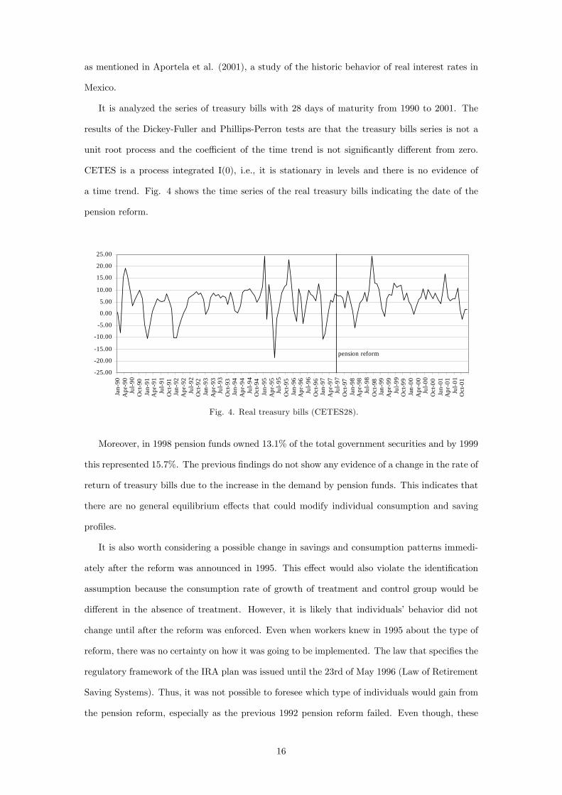
It is analyzed the series of treasury bills with 28 days of maturity from 1990 to 2001. The

results of the Dickey-Fuller and Phillips-Perron tests are that the treasury bills series is not a

unit root process and the coe¢ cient of the time trend is not signi�cantly di¤erent from zero.

CETES is a process integrated I(0), i.e., it is stationary in levels and there is no evidence of

a time trend. Fig. 4 shows the time series of the real treasury bills indicating the date of the

pension reform.

-25.00

-20.00

-15.00

-10.00

-5.00

0.00

5.00

10.00

15.00

20.00

25.00

Jan-

90A

pr-9

0Ju

l-90

Oct

-90

Jan-

91A

pr-9

1Ju

l-91

Oct

-91

Jan-

92A

pr-9

2Ju

l-92

Oct

-92

Jan-

93A

pr-9

3Ju

l-93

Oct

-93

Jan-

94A

pr-9

4Ju

l-94

Oct

-94

Jan-

95A

pr-9

5Ju

l-95

Oct

-95

Jan-

96A

pr-9

6Ju

l-96

Oct

-96

Jan-

97A

pr-9

7Ju

l-97

Oct

-97

Jan-

98A

pr-9

8Ju

l-98

Oct

-98

Jan-

99A

pr-9

9Ju

l-99

Oct

-99

Jan-

00A

pr-0

0Ju

l-00

Oct

-00

Jan-

01A

pr-0

1Ju

l-01

Oct

-01

pension reform

Fig. 4. Real treasury bills (CETES28).

Moreover, in 1998 pension funds owned 13.1% of the total government securities and by 1999

this represented 15.7%. The previous �ndings do not show any evidence of a change in the rate of

return of treasury bills due to the increase in the demand by pension funds. This indicates that

there are no general equilibrium e¤ects that could modify individual consumption and saving

pro�les.

It is also worth considering a possible change in savings and consumption patterns immedi-

ately after the reform was announced in 1995. This e¤ect would also violate the identi�cation

assumption because the consumption rate of growth of treatment and control group would be

di¤erent in the absence of treatment. However, it is likely that individuals�behavior did not

change until after the reform was enforced. Even when workers knew in 1995 about the type of

reform, there was no certainty on how it was going to be implemented. The law that speci�es the

regulatory framework of the IRA plan was issued until the 23rd of May 1996 (Law of Retirement

Saving Systems). Thus, it was not possible to foresee which type of individuals would gain from

the pension reform, especially as the previous 1992 pension reform failed. Even though, these

16

Page 17

e¤ects are tested using data from 1996, one year after the reform was approved. The estimates

show no e¤ect in consumption and savings, con�rming that matching identi�cation assumption

is satis�ed. These results are discussed in section 5.

Finally, another potential source of bias is the substitution to other type of annuitized income

during retirement. However, this would not a¤ect the estimates as in Mexico the coverage of

occupational and private pensions is very limited.

4.3. Control Group

The control or comparison group are workers contributing to ISSSTE (State Workers

Security and Social Services Institute), which is the second institute in terms of social security

coverage. It is mandatory for public sector workers and provides the same type of services as

IMSS. It has a PAYG pension plan which only su¤ered the 1992 pension reform that introduced

SAR, but it was not incorporated in the 1997 reform. Both pension schemes followed the same

course until IMSS�s was reformed in 1997 and ISSSTE�s remained unaltered.

Table 1 shows a comparison of the main features of the PAYG pension plans regulatory

framework. The retirement age and minimum years of contribution are the same in both groups.

Contribution is lower at ISSSTE. However, the employee pays a higher contribution, 3.5% in

comparison to 2.125% at IMSS. The method to compute ISSSTE�s pension is not much more

generous than IMSS�s. In 1996, ISSSTE�s average pension was 2.7 times the minimum wage and

at IMSS was 1.7 times the minimum wage.

Table 1Requirements and bene�ts of IMSS and ISSSTE pension schemes

IMSS (before 1997) ISSSTEEarly retirement age 60 60

Years of contribution 10 10

Contributions 10.5% 9.0%

Method to compute thepension

average wage of previous 5years to retirement

wage of previous year to retire-ment

Indexation of pension minimum wage of Mexico City minimum wage of Mexico City

In spite of ISSSTE covering public sector employees, their characteristics are similar to the

private sector for the following reasons. First, the public sector not only includes management

occupations but also laborers. Second, there was no civil service in the Mexican government.

Third, the labor regulatory framework provides the same conditions for public and private sector

workers in terms of job stability.

17

Page 18

Additionally, it is examined whether employees from ISSSTE switched to IMSS after the

pension reform. This may change the composition of the control group after the reform. It

would not a¤ect the treatment group because they correspond only to the transition generation.

It is found no evidence of migration from ISSSTE to IMSS after the pension reform as the number

of contributors have a steady increase per year by 1.3% between 1994 and 1998.

4.4. Data

The data is from the Mexican National Survey of Household Income and Expenditure

(ENIGH). This survey contains data on demographic and labor market characteristics of house-

hold members, income, and expenditure.11 It is a cross-sectional survey, which interviews are

conducted every 2 years during the third and fourth quarter. The surveys available with the

same methodology are from 1992 onwards. Each survey contains interviews of approximately

10,000 random households.

The surveys used are 1994, one year before the approval of the pension reform, 1996, one year

after the announcement, and 1998, one year after the enforcement. The sample includes head of

households contributing to IMSS or ISSSTE. IMSS�s 1998 sample was restricted to workers with

more than one year of tenure to include only the transition generation. Also, households who

reported zero non-durable consumption or income were excluded from the sample to avoid some

sources of measurement error.

Consumption includes nondurables and durables goods. Savings are obtained as the di¤erence

between income and consumption because they are not directly observed in the survey. Moreover,

there is limited information to estimate the �ow of �nancial savings and it is not possible to

measure the stock of wealth. Expenditure and income variables were de�ated by the National

Consumer�s price index with base year 1994. Another advantage of this survey is that the

treatment and control groups are administered the same questionnaire, and the de�nitions of

the variables are the same. The latter is an important characteristic of the sample when using

matching methods as mentioned in Heckman et al. (1997).

In addition, before the 1997 reform, IMSS had two types of enrolment: temporary and

mandatory. This analysis only includes mandatory workers because temporary workers did not

contribute to the pension plan. Temporary a¢ liates were only entitled to healthcare services and

11The survey reports household income and expenditure from the previous three months to the interview. Eachhousehold is interviewed with a questionnaire that captures household demographic characteristics, labor status,and less frequent purchased goods. After the interview, households �ll in an expenditure diary for a week toregister nondurable products.

18

Page 19

they were mainly seasonal workers.12 As the 1997 reform incorporated all workers to contribute

to the pension plan, temporary workers were eliminated from the 1998 sample.

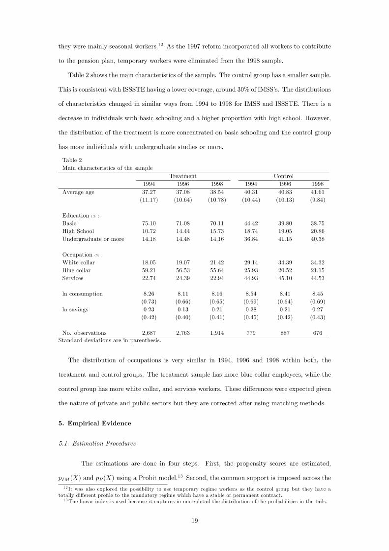
Table 2 shows the main characteristics of the sample. The control group has a smaller sample.

This is consistent with ISSSTE having a lower coverage, around 30% of IMSS�s. The distributions

of characteristics changed in similar ways from 1994 to 1998 for IMSS and ISSSTE. There is a

decrease in individuals with basic schooling and a higher proportion with high school. However,

the distribution of the treatment is more concentrated on basic schooling and the control group

has more individuals with undergraduate studies or more.

Table 2Main characteristics of the sample

Treatment Control1994 1996 1998 1994 1996 1998

Average age 37.27 37.08 38.54 40.31 40.83 41.61(11.17) (10.64) (10.78) (10.44) (10.13) (9.84)

Education (% )

Basic 75.10 71.08 70.11 44.42 39.80 38.75High School 10.72 14.44 15.73 18.74 19.05 20.86Undergraduate or more 14.18 14.48 14.16 36.84 41.15 40.38

Occupation (% )

White collar 18.05 19.07 21.42 29.14 34.39 34.32Blue collar 59.21 56.53 55.64 25.93 20.52 21.15Services 22.74 24.39 22.94 44.93 45.10 44.53

ln consumption 8.26 8.11 8.16 8.54 8.41 8.45(0.73) (0.66) (0.65) (0.69) (0.64) (0.69)

ln savings 0.23 0.13 0.21 0.28 0.21 0.27(0.42) (0.40) (0.41) (0.45) (0.42) (0.43)

No. observations 2,687 2,763 1,914 779 887 676Standard deviations are in parenthesis.

The distribution of occupations is very similar in 1994, 1996 and 1998 within both, the

treatment and control groups. The treatment sample has more blue collar employees, while the

control group has more white collar, and services workers. These di¤erences were expected given

the nature of private and public sectors but they are corrected after using matching methods.

5. Empirical Evidence

5.1. Estimation Procedures

The estimations are done in four steps. First, the propensity scores are estimated,

pIM (X) and pP (X) using a Probit model.13 Second, the common support is imposed across the12 It was also explored the possibility to use temporary regime workers as the control group but they have a

totally di¤erent pro�le to the mandatory regime which have a stable or permanent contract.13The linear index is used because it captures in more detail the distribution of the probabilities in the tails.

19

Page 20

4 cells by removing the units that have a propensity score for contribution and time period: a)

greater than the maximum or b) lower than the minimum of the comparisons groups. Third,

Nearest Neighbor and Kernel matching are computed to obtain the average e¤ect of the treatment

on the treated. Finally, the standard errors are estimated using the Bootstrap method.

One of the main estimation issues of the propensity score is the selection of enough observ-

able characteristics in order to assume that matched individuals do not di¤er signi�cantly by

unobservable characteristics. The propensity score includes the variables age, gender, education,

occupation, number of jobs of the head of household, number of children, number of household

total residents, geographical region, and community size. Other variables such as income, and

number of total working hours were not included because they could had been a¤ected by the

reform.

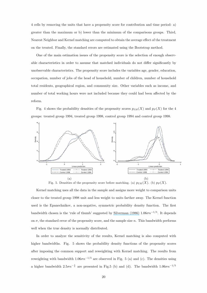
Fig. 4 shows the probability densities of the propensity scores pIM (X) and pP (X) for the 4

groups: treated group 1994, treated group 1998, control group 1994 and control group 1998.

0.2

.4.6

.8D

ensi

ty

-1 0 1 2Linear prediction

Treated 1998 Treated 1994Control 1998 Control 1994

0.5

11.

52

Den

sity

-2 -1 0 1Linear prediction

Treated 1998 Treated 1994Control 1998 Control 1994

(a) (b)Fig. 5. Densities of the propensity score before matching. (a) pIM (X). (b) pP (X).

Kernel matching uses all the data in the sample and assigns more weight to comparison units

closer to the treated group 1998 unit and less weight to units farther away. The Kernel function

used is the Epanechnikov, a non-negative, symmetric probability density function. The �rst

bandwidth chosen is the �rule of thumb�suggested by Silverman (1986) 1:06�n�1=5. It depends

on �; the standard error of the propensity score, and the sample size n. This bandwidth performs

well when the true density is normally distributed.

In order to analyze the sensitivity of the results, Kernel matching is also computed with

higher bandwidths. Fig. 5 shows the probability density functions of the propensity scores

after imposing the common support and reweighting with Kernel matching. The results from

reweighting with bandwidth 1:06�n�1=5 are observed in Fig. 5 (a) and (c). The densities using

a higher bandwidth 2:5�n�15 are presented in Fig.5 (b) and (d). The bandwidth 1:06�n�1=5

20

Page 21

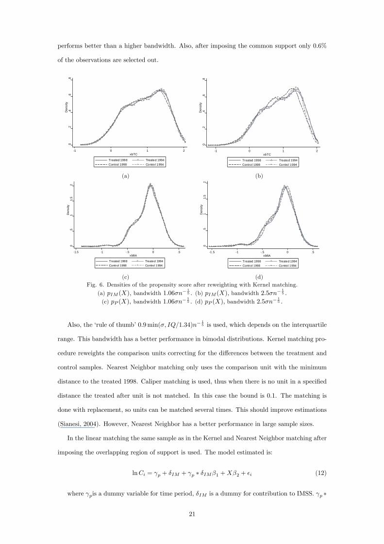
performs better than a higher bandwidth. Also, after imposing the common support only 0.6%

of the observations are selected out.0

.2.4

.6.8

Den

sity

-1 0 1 2xbTC

Treated 1998 Treated 1994Control 1998 Control 1994

0.2

.4.6

.8D

ensi

ty

-1 0 1 2xbTC

Treated 1998 Treated 1994Control 1998 Control 1994

(a) (b)

0.5

11.

52

Den

sity

-1.5 -1 -.5 0 .5xbBA

Treated 1998 Treated 1994Control 1998 Control 1994

0.5

11.

52

Den

sity

-1.5 -1 -.5 0 .5xbBA

Treated 1998 Treated 1994Control 1998 Control 1994

(c) (d)Fig. 6. Densities of the propensity score after reweighting with Kernel matching.

(a) pIM (X); bandwidth 1:06�n�15 . (b) pIM (X), bandwidth 2:5�n�

15 .

(c) pP (X); bandwidth 1:06�n�15 . (d) pP (X); bandwidth 2:5�n�

15 .

Also, the �rule of thumb�0:9min(�; IQ=1:34)n�15 is used, which depends on the interquartile

range. This bandwidth has a better performance in bimodal distributions. Kernel matching pro-

cedure reweights the comparison units correcting for the di¤erences between the treatment and

control samples. Nearest Neighbor matching only uses the comparison unit with the minimum

distance to the treated 1998. Caliper matching is used, thus when there is no unit in a speci�ed

distance the treated after unit is not matched. In this case the bound is 0.1. The matching is

done with replacement, so units can be matched several times. This should improve estimations

(Sianesi, 2004). However, Nearest Neighbor has a better performance in large sample sizes.

In the linear matching the same sample as in the Kernel and Nearest Neighbor matching after

imposing the overlapping region of support is used. The model estimated is:

lnCi = p + �IM + p � �IM�1 +X�2 + �i (12)

where pis a dummy variable for time period, �IM is a dummy for contribution to IMSS. p �

21

Page 22

�IM is the interaction term. X is a n�k matrix of household and head of family characteristics,

including a constant term.

In addition, to obtain the ATT for the di¤erent groups a¤ected by the pension reform, house-

holds were classi�ed by monthly labor income. Kernel, Nearest Neighbor and Linear matching

were computed for each threshold of income to analyze the heterogeneous e¤ects of the Mexican

pension reform.

5.3. Results

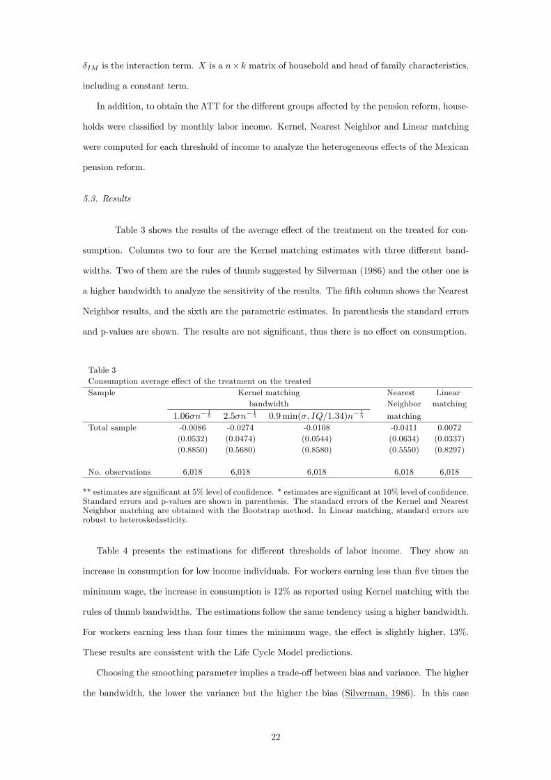
Table 3 shows the results of the average e¤ect of the treatment on the treated for con-

sumption. Columns two to four are the Kernel matching estimates with three di¤erent band-

widths. Two of them are the rules of thumb suggested by Silverman (1986) and the other one is

a higher bandwidth to analyze the sensitivity of the results. The �fth column shows the Nearest

Neighbor results, and the sixth are the parametric estimates. In parenthesis the standard errors

and p-values are shown. The results are not signi�cant, thus there is no e¤ect on consumption.

Table 3Consumption average e¤ect of the treatment on the treatedSample Kernel matching Nearest Linear

bandwidth Neighbor matching

1:06�n�15 2:5�n�

15 0:9min(�; IQ=1:34)n�

15 matching

Total sample -0.0086 -0.0274 -0.0108 -0.0411 0.0072(0.0532) (0.0474) (0.0544) (0.0634) (0.0337)(0.8850) (0.5680) (0.8580) (0.5550) (0.8297)

No. observations 6,018 6,018 6,018 6,018 6,018

** estimates are signi�cant at 5% level of con�dence. * estimates are signi�cant at 10% level of con�dence.Standard errors and p-values are shown in parenthesis. The standard errors of the Kernel and NearestNeighbor matching are obtained with the Bootstrap method. In Linear matching, standard errors arerobust to heteroskedasticity.

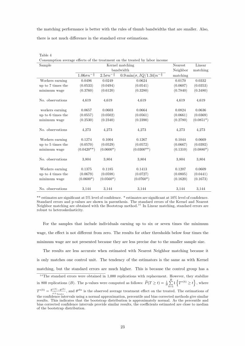
Table 4 presents the estimations for di¤erent thresholds of labor income. They show an

increase in consumption for low income individuals. For workers earning less than �ve times the

minimum wage, the increase in consumption is 12% as reported using Kernel matching with the

rules of thumb bandwidths. The estimations follow the same tendency using a higher bandwidth.

For workers earning less than four times the minimum wage, the e¤ect is slightly higher, 13%.

These results are consistent with the Life Cycle Model predictions.

Choosing the smoothing parameter implies a trade-o¤ between bias and variance. The higher

the bandwidth, the lower the variance but the higher the bias (Silverman, 1986). In this case

22

Page 23

the matching performance is better with the rules of thumb bandwidths that are smaller. Also,

there is not much di¤erence in the standard error estimations.

Table 4Consumption average e¤ects of the treatment on the treated by labor incomeSample Kernel matching Nearest Linear

bandwidth Neighbor matching

1:06�n�15 2:5�n�

15 0:9min(�; IQ=1:34)n�

15 matching

Workers earning 0.0496 0.0249 0.0624 0.0170 0.0332up to 7 times the (0.0533) (0.0494) (0.0541) (0.0607) (0.0353)minimum wage (0.3760) (0.6120) (0.3280) (0.7840) (0.3480)

No. observations 4,619 4,619 4,619 4,619 4,619

workers earning 0.0657 0.0603 0.0664 0.0824 0.0636up to 6 times the (0.0557) (0.0502) (0.0561) (0.0661) (0.0369)minimum wage (0.2530) (0.2340) (0.2390) (0.2780) (0.0851*)

No. observations 4,273 4,273 4,273 4,273 4,273

Workers earning 0.1274 0.1004 0.1267 0.1044 0.0669up to 5 times the (0.0570) (0.0529) (0.0572) (0.0667) (0.0392)minimum wage (0.0420**) (0.0600*) (0.0300**) (0.1310) (0.0880*)

No. observations 3,804 3,804 3,804 3,804 3,804

Workers earning 0.1375 0.1185 0.1413 0.1207 0.0609up to 4 times the (0.0679) (0.0598) (0.0727) (0.0805) (0.0441)minimum wage (0.0600*) (0.0560*) (0.0760*) (0.1620) (0.1673)

No. observations 3,144 3,144 3,144 3,144 3,144

** estimates are signi�cant at 5% level of con�dence. * estimates are signi�cant at 10% level of con�dence.Standard errors and p-values are shown in parenthesis. The standard errors of the Kernel and NearestNeighbor matching are obtained with the Bootstrap method.14 In Linear matching, standard errors arerobust to heteroskedasticity.

For the samples that include individuals earning up to six or seven times the minimum

wage, the e¤ect is not di¤erent from zero. The results for other thresholds below four times the

minimum wage are not presented because they are less precise due to the smaller sample size.

The results are less accurate when estimated with Nearest Neighbor matching because it

is only matches one control unit. The tendency of the estimators is the same as with Kernel

matching, but the standard errors are much higher. This is because the control group has a

14The standard errors were obtained in 1,000 replications with replacement. However, they stabilize

in 800 replications (B). The p-values were computed as follows: bP (T � t) = 1B

BPb=1

1nT �(b) � t

o; where

T �(b) = ��(b)��obs_s:e:boots

; and �obs is the observed average treatment e¤ect on the treated. The estimations of

the con�dence intervals using a normal approximation, percentile and bias corrected methods give similarresults. This indicates that the bootstrap distribution is approximately normal. As the percentile andbias corrected con�dence intervals provide similar results, the coe¢ cients estimated are close to medianof the bootstrap distribution.

23

Page 24

smaller sample size than the treatment group and some units are matched several times, causing

an increase in the variance.

The linear di¤erence-in-di¤erences estimates show a signi�cant positive e¤ect of 6.6% for

workers earning up to �ve times the minimum wage and 6.3% for the sample with workers

earning up to six times the minimum wage. The estimates are lower than Kernel matching. The

di¤erence between the parametric and matching estimations is the weighting system.

Multivariate linear regression produces estimates that are a weighted average of the covari-

ates. The value of the coe¢ cients depends on the distribution of the independent variables and

the heterogeneity of the ATT (Angrist and Krueger, 1999). Additionally, it imposes a linear

functional form. Matching estimations are more accurate because the weighting system is more

adaptable.

Table 5 shows the e¤ects on savings and labor income. The average e¤ect of the treatment

on the treated on savings is estimated as the bootstrap di¤erence between after tax household

income and consumption. Data on savings is not directly observed because the ENIGH mainly

provides household income and expenditure.

The results show a decline on savings for individuals earning less than �ve times the minimum

wage by 8.8% with 1:06�n�15 bandwidth. The estimates for labor income are not signi�cant.

The pension reform e¤ect in labor income is so small that does not have any impact. There is

no e¤ect on wages. This also suggests no changes in number of working hours after the pension

reform, disregarding labor supply e¤ects.

24

Page 25

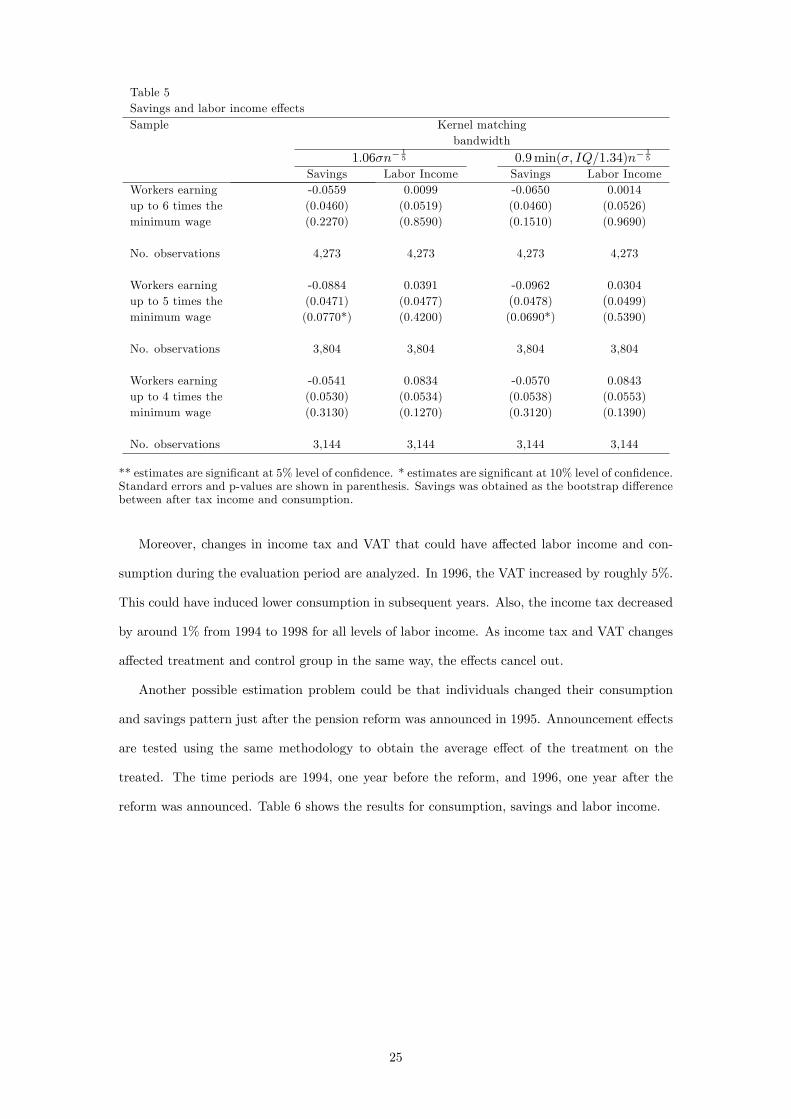
Table 5Savings and labor income e¤ectsSample Kernel matching

bandwidth

1:06�n�15 0:9min(�; IQ=1:34)n�

15

Savings Labor Income Savings Labor IncomeWorkers earning -0.0559 0.0099 -0.0650 0.0014up to 6 times the (0.0460) (0.0519) (0.0460) (0.0526)minimum wage (0.2270) (0.8590) (0.1510) (0.9690)

No. observations 4,273 4,273 4,273 4,273

Workers earning -0.0884 0.0391 -0.0962 0.0304up to 5 times the (0.0471) (0.0477) (0.0478) (0.0499)minimum wage (0.0770*) (0.4200) (0.0690*) (0.5390)

No. observations 3,804 3,804 3,804 3,804

Workers earning -0.0541 0.0834 -0.0570 0.0843up to 4 times the (0.0530) (0.0534) (0.0538) (0.0553)minimum wage (0.3130) (0.1270) (0.3120) (0.1390)

No. observations 3,144 3,144 3,144 3,144

** estimates are signi�cant at 5% level of con�dence. * estimates are signi�cant at 10% level of con�dence.Standard errors and p-values are shown in parenthesis. Savings was obtained as the bootstrap di¤erencebetween after tax income and consumption.

Moreover, changes in income tax and VAT that could have a¤ected labor income and con-

sumption during the evaluation period are analyzed. In 1996, the VAT increased by roughly 5%.

This could have induced lower consumption in subsequent years. Also, the income tax decreased

by around 1% from 1994 to 1998 for all levels of labor income. As income tax and VAT changes

a¤ected treatment and control group in the same way, the e¤ects cancel out.

Another possible estimation problem could be that individuals changed their consumption

and savings pattern just after the pension reform was announced in 1995. Announcement e¤ects

are tested using the same methodology to obtain the average e¤ect of the treatment on the

treated. The time periods are 1994, one year before the reform, and 1996, one year after the

reform was announced. Table 6 shows the results for consumption, savings and labor income.

25

Page 26

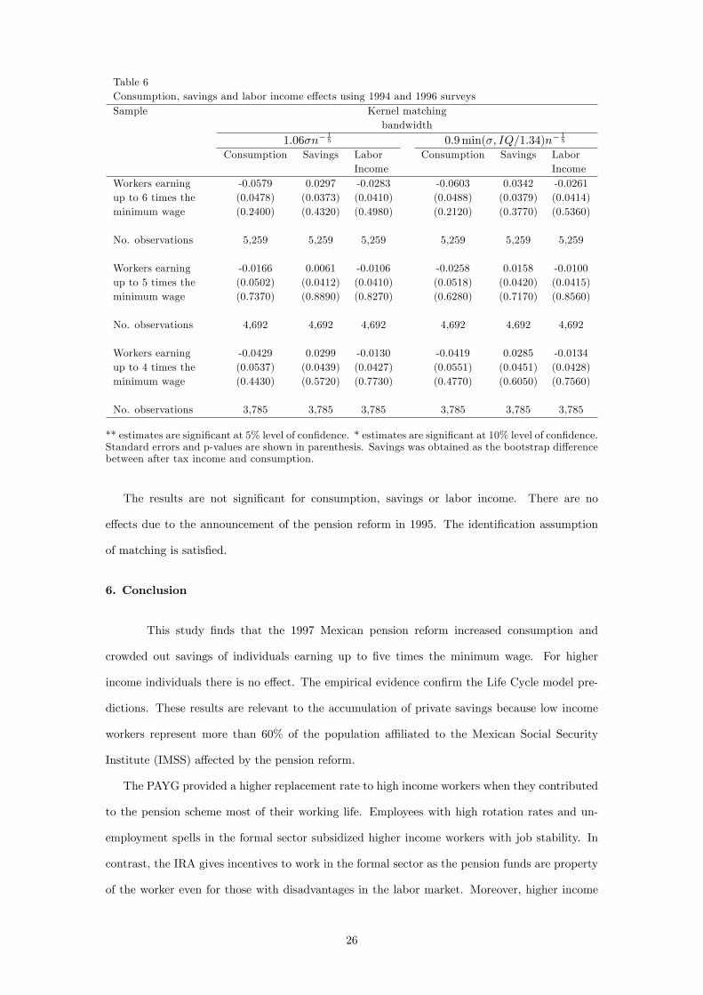
Table 6Consumption, savings and labor income e¤ects using 1994 and 1996 surveysSample Kernel matching

bandwidth

1:06�n�15 0:9min(�; IQ=1:34)n�

15

Consumption Savings LaborIncome

Consumption Savings LaborIncome

Workers earning -0.0579 0.0297 -0.0283 -0.0603 0.0342 -0.0261up to 6 times the (0.0478) (0.0373) (0.0410) (0.0488) (0.0379) (0.0414)minimum wage (0.2400) (0.4320) (0.4980) (0.2120) (0.3770) (0.5360)

No. observations 5,259 5,259 5,259 5,259 5,259 5,259

Workers earning -0.0166 0.0061 -0.0106 -0.0258 0.0158 -0.0100up to 5 times the (0.0502) (0.0412) (0.0410) (0.0518) (0.0420) (0.0415)minimum wage (0.7370) (0.8890) (0.8270) (0.6280) (0.7170) (0.8560)

No. observations 4,692 4,692 4,692 4,692 4,692 4,692

Workers earning -0.0429 0.0299 -0.0130 -0.0419 0.0285 -0.0134up to 4 times the (0.0537) (0.0439) (0.0427) (0.0551) (0.0451) (0.0428)minimum wage (0.4430) (0.5720) (0.7730) (0.4770) (0.6050) (0.7560)

No. observations 3,785 3,785 3,785 3,785 3,785 3,785

** estimates are signi�cant at 5% level of con�dence. * estimates are signi�cant at 10% level of con�dence.Standard errors and p-values are shown in parenthesis. Savings was obtained as the bootstrap di¤erencebetween after tax income and consumption.

The results are not signi�cant for consumption, savings or labor income. There are no

e¤ects due to the announcement of the pension reform in 1995. The identi�cation assumption

of matching is satis�ed.

6. Conclusion

This study �nds that the 1997 Mexican pension reform increased consumption and

crowded out savings of individuals earning up to �ve times the minimum wage. For higher

income individuals there is no e¤ect. The empirical evidence con�rm the Life Cycle model pre-

dictions. These results are relevant to the accumulation of private savings because low income

workers represent more than 60% of the population a¢ liated to the Mexican Social Security

Institute (IMSS) a¤ected by the pension reform.

The PAYG provided a higher replacement rate to high income workers when they contributed

to the pension scheme most of their working life. Employees with high rotation rates and un-

employment spells in the formal sector subsidized higher income workers with job stability. In

contrast, the IRA gives incentives to work in the formal sector as the pension funds are property

of the worker even for those with disadvantages in the labor market. Moreover, higher income

26

Page 27

workers obtain a fair pension linked to their contributions. It is also worth noticing that a �aw

of the IRA design is the voluntary option whose aim to promote savings has been very limited.

The empirical results show no evidence of precautionary savings e¤ects for workers with a

labor income above �ve times the minimum wage. For workers earning up to �ve times the

minimum wage, some of the increase in consumption may be due to a higher credibility under

the IRA plan. It is possible to suggest that low income workers may have greater expectations

of the IRA scheme while higher income individuals do not perceive any substantial change.

Some initial policy recommendations derived from this research are as follows. The IRA

scheme could be modi�ed to promote household savings jointly with other labor market policies.

Speci�c features to be included in the IRA are �scal exemptions to employers, and employees

for voluntary contributions, targeting groups with low levels of saving. Voluntary contributions

procedures could be simpli�ed.

Furthermore, individuals should be provided with information about the advantages of saving

in the IRA. The spouse and other household members may be given access to save in the voluntary

scheme to provide middle and low income families a saving option with high earnings. Finally,

labor market policies may be focused in extending working lives in the formal sector to incentive

a higher accumulation of retirement savings.

Appendix A

A.1. 1992 Pension Reform

The 1992 reform created complementary individual retirement accounts to the PAYG

scheme. This reform raised employer�s contribution by 2%, which was managed by the Central

Bank in the system denominated SAR (Retirement Saving System). The SAR guaranteed an

annual minimum real rate of return of 2% and earnings were not taxed. The investment portfolio

was restricted to only government bonds. Also voluntary contributions were feasible but they

were not registered separately to the mandatory. Thus, in practice there were no voluntary

contributions.

The funds accumulated in the complementary individual account were given to the employee

as a one-o¤ payment at retirement. The SAR system was valid from 1992 to 1997. The SAR

pension wealth is worth 10.6% of employees annual salary after contributing for �ve years. The

lump sum is equivalent to 6.3% and 2.0% of the annual salary after contributing for three or

one year, respectively. The pension wealth received from the 1992 individual retirement account

27

Page 28

is quite small even when the individual contributed during the whole period the system was

enforced.

Moreover, this reform failed due to many management problems: a) a poor regulatory frame-

work, and b) multiplicities of accounts. The commission in charge of the accountability of the

retirement saving system (CONSAR) began operations 2 years after the pension reform was

introduced, until the 13th of July 1994. Also commercial banks which did the record keeping

and transferred contributions to the Central Bank, did not have incentives to provide an e¢ cient

service because the fee charged was very poor.

The most inadequate feature was that only the employer made contributions and selected

the registration bank. This led to the perception that the individual account was simply an

additional tax. The worker did not know the balance of the individual account and nor generally

the registration bank. Besides, when the worker switched jobs, the new employer did not have

incentives to track the individual account of the previous job.

All these factors led to multiple individual accounts for the employee. Diminishing the impact

of SAR at retirement mainly for individuals with higher rotation rates. Therefore, the reform

was swiftly considered to be a failure.

A.2. 1997 Pension Reform

A.2.1. Contributions

Contributions to the pension plan did not change for the employer and employee, only

for the government by the social quota as shown in the third row of Table A.1. The social quota is

equivalent to 5.5% of the minimum wage of Mexico City adjusted to in�ation with the National

Consumer�s Price Index (NCPI). Also, Table A.1. shows the change in the concentration of

resources from the PAYG to the IRA after the pension reform.

Table A.1.Contributions of the pension scheme (% of employee�s wage)Scheme Before 1997 After 1997

Employer Employee Government Employer Employee GovernmentPAYG 5.950 2.125 0.425 2.800 1.000 0.200

IRA 2.000 � � 5.150 1.1250.225 +

social quota

Total 7.950 2.125 0.425 7.950 2.1250.425 +

social quotaHousing 5.000 � � 5.000 � �

Worker�s wage is de�ned as the nominal wage plus all the labor bene�ts given to the employee, suchas commissions, extra-hours, meals, uniforms, among others. The PAYG plan before 1997 was theDisability, Old Age, Severance and Life Insurance (IVCM). After 1997, contributions managed by IMSS

28

Page 29

correspond to health services for pensioners (1.05% employer, 0.625% employee, and 0.125% government)and disability and life insurance (1.75% employer, 0.375% employee, and 0.075% government). TheIRA contributions before 1997 represent the 1992 complementary individual account. After 1997, IRAcontributions are managed in the subaccounts: Retirement (2.00%), and Severance and Old age (3.15%).In addition, after 1997, housing contributions are used to compute the pension at retirement. However,they are still managed by INFONAVIT, an institute in charge of providing housing credits.

In the �rst row of Table A.2. is shown the change in healthcare services contributions. Before

1997, the employer and worker contributed 11.875% of worker�s wage. After 1997, for workers

with a monthly earning below three times the minimum wage, the employer contributes 13.9% of

the minimum wage of Mexico City. For workers earning above three times the minimum wage,

the employer and employee contributes an additional 8% of the di¤erence between the worker�s

wage and three times the minimum wage.

Table A.2.Contributions to other services provided by IMSS (% worker�s wage)Scheme Before 1997 After 1997

Employer Employee Government Employer Employee Governmentbelow three times the minimum wagea:

Healthcare 8.750 3.125 0.625 13.900 � 13.900amount above three timesthe minimum wage:+ 6.000 + 2.000 �

Nurseries 1.000 � � 1.000 � �

Work Injuries Industry � � Firm � �Compensation accident rate accident rate

aThis contribution is paid as a percentage of a minimum wage of Mexico city.The Income Tax Law determines that workers earning the minimum wage do not pay taxes, all contri-butions are covered by the employer. The healthcare services plan is denominated Illness and MaternityInsurance (SEM).

Moreover, Table A.2. shows a comparison of the contributions to the other services provided

by IMSS. Only the Work Injuries Compensation contribution changed for the employers.

A.2.2. Pension Wealth

The present value of pensions were computed under the PAYG and IRA rules. The

assumptions are that individuals retire at age 60 with 25 years of contribution. It was chosen

early retirement because there are no incentives to wait until normal retirement.

The annual minimum wage in�ationary loss is 6.4% computed with data from INEGI (2003).

The discount rate assumed is 1%. Also, the simulations use IMSS�s life expectancy assumptions.

These are 93 years old for men and 87 for women. Men has a higher life expectancy because it is

included a period after the death of pensioner where the pension is provided to the dependents

such as the widow or children under age 16.

29

Page 30

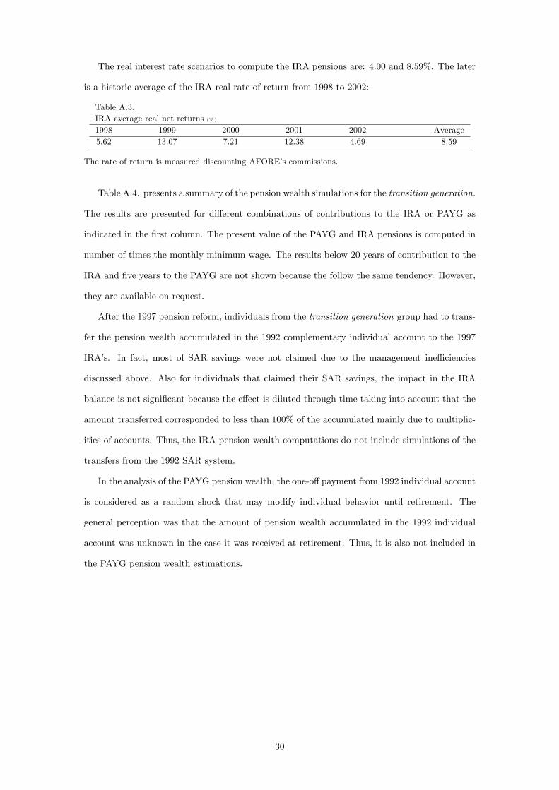
The real interest rate scenarios to compute the IRA pensions are: 4.00 and 8.59%. The later

is a historic average of the IRA real rate of return from 1998 to 2002:

Table A.3.IRA average real net returns (% )

1998 1999 2000 2001 2002 Average5.62 13.07 7.21 12.38 4.69 8.59

The rate of return is measured discounting AFORE�s commissions.

Table A.4. presents a summary of the pension wealth simulations for the transition generation.

The results are presented for di¤erent combinations of contributions to the IRA or PAYG as

indicated in the �rst column. The present value of the PAYG and IRA pensions is computed in

number of times the monthly minimum wage. The results below 20 years of contribution to the

IRA and �ve years to the PAYG are not shown because the follow the same tendency. However,

they are available on request.

After the 1997 pension reform, individuals from the transition generation group had to trans-

fer the pension wealth accumulated in the 1992 complementary individual account to the 1997

IRA�s. In fact, most of SAR savings were not claimed due to the management ine¢ ciencies

discussed above. Also for individuals that claimed their SAR savings, the impact in the IRA

balance is not signi�cant because the e¤ect is diluted through time taking into account that the

amount transferred corresponded to less than 100% of the accumulated mainly due to multiplic-

ities of accounts. Thus, the IRA pension wealth computations do not include simulations of the

transfers from the 1992 SAR system.

In the analysis of the PAYG pension wealth, the one-o¤payment from 1992 individual account

is considered as a random shock that may modify individual behavior until retirement. The

general perception was that the amount of pension wealth accumulated in the 1992 individual

account was unknown in the case it was received at retirement. Thus, it is also not included in

the PAYG pension wealth estimations.

30

Page 31

TableA.4.

PresentvalueofpensionsatretirementunderthePAYG

andIRAforthetransitiongeneration

Years

of

contribution

totheplan

Pension

wealth

Realinterest

rate

scenarios

IRA

PAYG

4.00

8.59

4.00

8.59

4.00

8.59

4.00

8.59

4.00

8.59

4.00

8.59

4.00

8.59

4.00

8.59

4.00

8.59

24

1IRA

347.88

347.88

347.88

347.88

347.88

347.88

347.88

347.88

347.88

381.41

347.88

448.55

347.88

515.70

351.79

582.85

680.02

1120.03

PAYG

150.81

150.81

158.54

158.54

223.02

223.02

275.16

275.16

327.63

327.63

380.16

380.16

440.10

440.10

502.98

502.98

1005.95

1005.95

Select

IRA

IRA

IRA

IRA

IRA

IRA

IRA

IRA

IRA

IRA

PAYG

IRA

PAYG

IRA

PAYG

IRA

PAYG

IRA

23

2IRA

347.88

347.88

347.88

347.88

347.88

347.88

347.88

347.88

347.88

352.43

347.88

414.62

347.88

476.81

347.88

539.00

650.43

1036.53

PAYG

150.81

150.81

158.54

158.54

223.02

223.02

275.16

275.16

327.63

327.63

380.16

380.16

440.10

440.10

502.98

502.98

1005.95

1005.95

Select

IRA

IRA

IRA

IRA

IRA

IRA

IRA

IRA

IRA

IRA

PAYG

IRA

PAYG

IRA

PAYG

IRA

PAYG

IRA

22

3IRA

347.88

347.88

347.88

347.88

347.88

347.88

347.88

347.88

347.88

347.88

347.88

383.37

347.88

441.00

347.88

498.63

621.98

959.65

PAYG

150.81

150.81

158.54

158.54

223.02

223.02

275.16

275.16

327.63

327.63

380.16

380.16

440.10

440.10

502.98

502.98

1005.95

1005.95

Select

IRA

IRA

IRA

IRA

IRA

IRA

IRA

IRA

IRA

IRA

PAYG

IRA

PAYG

IRA

PAYG

PAYG

PAYG

PAYG

21

4IRA

347.88

347.88

347.88

347.88

347.88

347.88

347.88

347.88

347.88

347.88

347.88

354.60

347.88

408.02

347.88

461.45

594.62

888.84

PAYG

150.81

150.81

158.54

158.54

223.02

223.02

275.16

275.16

327.63

327.63

380.16

380.16

440.10

440.10

502.98

502.98

1005.95

1005.95

Select

IRA

IRA

IRA

IRA

IRA

IRA

IRA

IRA

IRA

IRA

PAYG

PAYG

PAYG

PAYG

PAYG

PAYG

PAYG

PAYG

20

5IRA

347.88

347.88

347.88

347.88

347.88

347.88

347.88

347.88

347.88

347.88

347.88

347.88

347.88

377.66

347.88

427.21

568.32

823.64

PAYG

150.81

150.81

158.54

158.54

223.02

223.02

275.16

275.16

327.63

327.63

380.16

380.16

440.10

440.10

502.98

502.98

1005.95

1005.95

Select

IRA

IRA

IRA

IRA

IRA

IRA

IRA

IRA

IRA

IRA

PAYG

PAYG

PAYG

PAYG

PAYG

PAYG

PAYG

PAYG

12

34

56

78

16

Monthly

laborincome

31

Page 32

References

Angrist, J., Krueger, A., 1999. Empirical Strategies in Labor Economics, in: Arrow, K.S., Intriligator,

M.D. (Eds.), Handbook of Labor Economics, Vol. 3A. Elsevier, Amsterdam, pp. 1277�1366.

Aportela, F., Ardavín, J.A., Cruz, Y, 2001. Comportamiento Histórico de las Tasas de Interés Reales en

México, 1951-2001. Mexican Central Bank Working Paper 2001-05.

Attanasio, O., Brugiavini, A., 2003. Social Security and Households�Saving. The Quarterly Journal of

Economics 118, 3, 1075�1120.

Attanasio, O., Hoynes, H., 2000. Di¤erential Mortality and Wealth Accumulation. The Journal of

Human Resources 35, 1, 1�29.

Attanasio, O., Rohwedder, S., 2003. Pension Wealth and Household Saving: Evidence from Pension

Reforms in the United Kingdom. The American Economic Review 93, 5, 1499�1521.

Blundell, R., Costa Dias, M., 2002. Alternative Approaches to Evaluation in Empirical Microeconomics.

IFS-CEMMAP Working Paper CWP10/02.

Blundell, R., Costa Dias, M., Meghir, C., Van Reenen, J., 2004. Evaluating the Employment Impact of

a Mandatory Job Search Program. Journal of the European Economic Association, 2, 4, 569�606.

Efron, B., Tibshirani, R.J., 1993. An Introduction to the Bootstrap. Chapman & Hall, London.

Euwals, R., 2000. Do Mandatory Savings Decrease Household Savings? Evidence for the Netherlands.

IZA Discussion Paper No. 113.

Feldstein, M., 1974. Social Security, Induced Retirement, and Aggregate Capital Accumulation. The

Journal of Political Economy 82, 5, 905�926.

Gill, I., Packard, T., Yermo, J., 2004. Keeping the Promise of Social Security in Latin America. The

World Bank, Washington.

Gustman, A.L., Steinmeier, T.L., 1998. E¤ects of Pensions on Savings: Analysis with data from the

Health and Retirement Study. NBER Working Paper 6681.

Heckman, J., Ichimura, H., Todd, P., 1997. Matching As An Econometric Evaluation Estimator: Evi-

dence from Evaluating a Job Training Programme. Review of Economic Studies 64, 605�654.

Lindbeck, A., Persson, M., 2003. The Gains from Pension Reform. Journal of Economic Literature, 41,

1, 74�112.

Maloney, W.F., 2002. Distortion and Protection in the Mexican Labor Market. CREDPR Working

Paper 138.

Marrufo, G., 2001. The Incidence of Social Security Regulation in Economies with Partial Compliance:

Evidence from the Reform in Mexico. University of Chicago, Mimeo.

32

Page 33

Mesa-Lago, C., 2001. Structural reform of social security pensions in Latin America: Models, character-

istics, results and conclusions. International Social Security Review 54, 4, 67�92.

Mesa-Lago, C., 2004. La Reforma de Pensiones en América Latina. Modelos y características, mitos

y desempeños, y lecciones, in: Hujo, K., Mesa-Lago, C., Nitsch, M. (Eds.), Públicos o privados? Los

sistemas de pensiones en América Latina después de dos décadas de reformas. Nueva Sociedad, Caracas,

pp. 21�56.

Orszag, P., Stiglitz, J., 1999. Rethinking Pension Reform: Ten Myths About Social Security Systems, in:

conference New Ideas About Old Age Security. The World Bank, Washington, D.C., September 14-15.

Rosenbaum, P.R., Rubin, D.B., 1983. The central role of the propensity score in observational studies

for causal e¤ects. Biometrika 70, 41�55.

Sales, C., Solís, F., Villagómez, A., 1996. Pension System Reform: The Mexican Case. NBER Working

Paper 5780.

Sianesi, B., 2004. An evaluation of the Swedish system of active labour market programs in the 1990s�.

The Review of Economics and Statistics, 86, 1, 133�155.

Silverman, B.W., 1986. Density Estimation for Statistics and Data Analysis. Chapman & Hall, London.

Solís, F., Villagómez, A., 1999. Las Pensiones, in: Solís, F., Villagómez, A. (Eds.), La Seguridad Social

en México. Fondo de Cultura Económica, Mexico, pp. 103�159.

33