PEAT8002 - SEISMOLOGY Lecture 14: Free Oscillations Irses.anu.edu.au/~nick/teachdoc/lecture14.pdf · PEAT8002 - SEISMOLOGY Lecture 14: Free Oscillations I Nick Rawlinson Research

PEAT8002 - SEISMOLOGYLecture 14: Free Oscillations I

Nick Rawlinson

Research School of Earth SciencesAustralian National University

Free oscillations IIntroduction

Like a stretched string on a guitar, an elastic spheresupports standing waves. In seismology, these are knownas free oscillations or normal modes, and arecharacterises by a discrete spectrum.Only specific frequencies are permitted, corresponding tointegral numbers of wavelengths in the 3 orthogonaldirections (r , θ,Φ).These oscillations correspond to standing surface waves ofthe longest possible wavelength and lowest frequency(periods up to about 1 hour).The longest period oscillations are only excited in ameasurable way by the largest earthquakes, and it was notuntil the 1960 Chile earthquake that they wereunambiguously identified on long-period seismograms.

Free oscillations IIntroduction

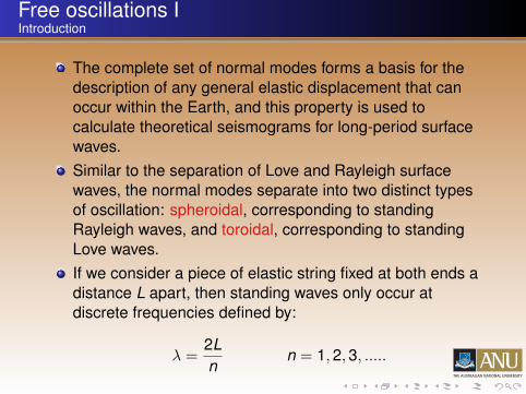
The complete set of normal modes forms a basis for thedescription of any general elastic displacement that canoccur within the Earth, and this property is used tocalculate theoretical seismograms for long-period surfacewaves.Similar to the separation of Love and Rayleigh surfacewaves, the normal modes separate into two distinct typesof oscillation: spheroidal, corresponding to standingRayleigh waves, and toroidal, corresponding to standingLove waves.If we consider a piece of elastic string fixed at both ends adistance L apart, then standing waves only occur atdiscrete frequencies defined by:

λ =2Ln

n = 1, 2, 3, .....

Free Oscillations IIntroduction

In this case, n = 1 defines the fundamental mode.

L

λ


The figure below demonstrates the concept of spheroidalmodes. These are equivalent to standing Rayleigh waveswith coupled P-SV motion.

Period = 54 minutesFundamental mode = "football mode"

Spheroidal mode Simplest mode = "breathing"Period = 20 minutes


The Figure below demonstrates the concept of torsionalmodes. The simplest torsional mode corresponds to arotating Earth, which is of no interest. The next modeinvolves two hemispheres moving in opposite directions.

Torsional modes Simplest torsional mode

Free Oscillations ISeparation of modes

We previously used Helmholtz’ theorem to show theseparation of P and S waves:

u = ∇Φ +∇×Ψ

In the above equation, u is displacement, Φ is the scalarpotential of the displacement field, and Ψ is the vectorpotential of the displacement field.This theorem can be slightly modified for use in sphericalanalysis, as we can separate the vector potential into theorthogonal radial and horizontal components:

Ψ = T r̂ +∇× (Sr̂)


Thus, the displacement can be written:

u = ∇Φ +∇× T r̂ +∇×∇× (Sr̂)

Now there are three scalar potentials, T , giving thetorsional mode oscillations (SH type displacement), and Φand S, giving the spheroidal mode oscillations (coupled Pand SV displacements).From earlier, the Navier equation of motion was written as:

ρ∂2u∂t2 = (λ + µ)∇θ + µ∇2u + ρ∇U

where ∇U is the gravitational acceleration.


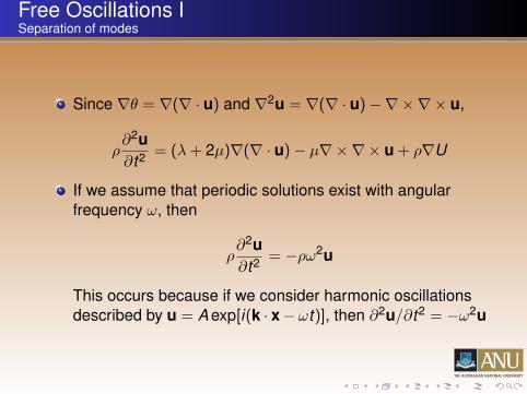
Since ∇θ = ∇(∇ · u) and ∇2u = ∇(∇ · u)−∇×∇× u,

ρ∂2u∂t2 = (λ + 2µ)∇(∇ · u)− µ∇×∇× u + ρ∇U

If we assume that periodic solutions exist with angularfrequency ω, then

ρ∂2u∂t2 = −ρω2u

This occurs because if we consider harmonic oscillationsdescribed by u = A exp[i(k · x− ωt)], then ∂2u/∂t2 = −ω2u


Substitution into the Navier equation gives:

(λ + 2µ)∇(∇ · u)− µ∇×∇× u + ρ∇U = −ρω2u (1)

We now substitute u = ∇Φ +∇× T r̂ +∇×∇× (Sr̂) intoequation (1).The separate components involving displacement can beconsidered as follows:

∇ · u = ∇ · ∇Φ +∇ · (∇× T r̂) +∇ · (∇×∇× (Sr̂)) = ∇2Φ

noting that the divergence of a curl is zero.


The next term is:

∇×∇× u = ∇×∇× (∇Φ) + (∇×)3T r̂ + (∇×)4(Sr̂)= (∇×)3T r̂ + (∇×)4(Sr̂)

noting that the curl of a gradient is zero.Substitution into Equation (1) therefore gives:

−ρω2u = (λ + 2µ)∇(∇2Φ)− µ[(∇×)3T r̂ + (∇×)4(Sr̂)] + ρ∇U

If we now take the divergence (∇·) of this expression:

∇ · (−ρω2u) = ∇ · (λ + 2µ)∇(∇2Φ)

−∇ · µ[(∇×)3T r̂ + (∇×)4(Sr̂)] +∇ · ρ∇U


The first term ∇ · (−ρω2u) = −ρω2∇2Φ since ∇ · u = ∇2Φ.The third term ∇ · µ[(∇×)3T r̂ + (∇×)4(Sr̂)] = 0 becausethe divergence of a curl is zero.The final term ∇ · ρ∇U = ρ∇2U ≈ 0, if we assume thesecond derivative of U is negligible (variations in bodyforce ignored).Putting these terms together gives:

ρω2∇2Φ + (λ + 2µ)∇4Φ = 0

The above equation is for a scalar potential Φ with P-typeoscillation.


If we now take the curl (∇×) of Equation (1),

∇× (ρω2u) = ∇× (µ∇×∇× u)−∇× (λ + 2µ)∇(∇ · u)

−∇× (ρ∇U)

The last two terms are zero because the curl of a gradientis zero.Since ∇× u = ∇×∇× T r̂ + (∇×)3Sr̂, then

(∇×)3u = (∇×)4T r̂ + (∇×)5Sr̂

This allows us to form the following equation:

ρω2[(∇×)2T r̂+(∇×)3Sr̂] = µ(∇×)4T r̂+µ(∇×)5Sr̂ (2)


If we now take the dot product of Equation (2) with r̂, then

ρω2r̂ · [(∇×)2T r̂ + (∇×)3Sr̂] = µr̂ · (∇×)4T r̂ + µr̂ · (∇×)5Sr̂

We now make use of the following results from vectoralgebra:

r̂ · ∇ × (∇×)2n(r̂f ) = 0, n > 0

r̂ · ∇ ×∇× (r̂f ) =−1r2 ∇h

2f

r̂ · (∇×)2n(r̂f ) =(−1)2

r∇2(n−1)∇h

2(

fr

)where f = f (r , θ, φ) is a scalar function and ∇h

2 is thehorizontal component of ∇.


It therefore follows that r̂ · (∇×)3Sr̂ = 0 andr̂ · (∇×)5Sr̂ = 0.The above equation then reduces to:

−ρω2

r2 ∇h2T =

µ

r∇2∇h

2 Tr

Noting that r is not operated on by ∇h2, we can write this

equation as

ρω2

r∇h

2(

Tr

)+

µ

r∇2∇h

2(

Tr

)= 0

The above equation is for a torsional potential (SH typeoscillation).


If we now take the curl of equation (2), then

ρω2[(∇×)3T r̂ + (∇×)4Sr̂] = µ(∇×)5T r̂ + µ(∇×)6Sr̂

The terms involving T are equal to zero because they arepremultiplied by (∇×)n where n is an odd number.If we take the dot product of both sides of the equation withr̂, the the two terms for S become:

r̂·(∇×)4Sr̂ =1r∇2∇h

2(

Sr

)r̂·(∇×)6Sr̂ = −1

r∇4∇h

2(

Sr

)We thus end with an equation for the spheroidal potential(SV oscillation):

ρω2∇2∇h2(

Sr

)+ µ∇4∇h

2(

Sr

)= 0


Thus, we have derived three equations:

ρω2∇2Φ + (λ + 2µ)∇4Φ = 0 (a)

ρω2

r∇h

2(

Tr

)+

µ

r∇2∇h

2(

Tr

)= 0 (b)

ρω2∇2∇h2(

Sr

)+ µ∇4∇h

2(

Sr

)= 0 (c)

Each of these equations may be written in the form:(ω

c

)2f +∇2f = 0

which is often referred to as Helmholtz’ equation.


The Helmholtz’ equation is the time-independent form of awave equation, derived by assuming a separation ofvariables (in this case displacement u).In the case of Equation (a), c is the P-wave velocity, givenby:

α =

√λ + 2µ

ρwhere f = ∇2Φ

In the case of Equation (b), c is the S-wave velocity, givenby:

β =

√µ

ρwhere f = ∇h

2(T/r)

In the case of Equation (c), c is the S-wave velocity, givenby:

β =

√µ

ρwhere f = ∇2∇h

2(S/r)


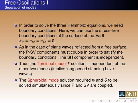
In order to solve the three Helmholtz equations, we needboundary conditions. Here, we can use the stress-freeboundary conditions at the surface of the Earthσrr = σrθ = σrφ = 0.As in the case of plane waves reflected from a free surface,the P-SV components must couple in order to satisfy theboundary conditions. The SH component is independent.Thus, the Torsional mode T solution is independent of theother two modes (implies long period standing Lovewaves).The Spheroidal mode solution required Φ and S to besolved simultaneously since P and SV are coupled.


In the special case of a fluid sphere, T and S vanish (sinceu = ∇Φ in this case).Therefore, dilatation θ = ∇2Φ. Since the pressurep = σkk/3 and σij = λθδij , then

θ =pλ

=pκ

where κ is the adiabatic bulk modulus.Thus, the pressure field of a free oscillation must directlysatisfy Helmholtz’ equation:(ω

c

)2p +∇2p = 0

Free Oscillations ISolving Helmholtz’ Equation

From before, we have Helmholtz’ equation written as(ω

c

)2f +∇2f = 0 (3)

where f = f (r , θ, φ). Solution in 3-D spherical geometrycan be expressed in terms of spherical harmonics.Note that we have assumed an oscillatory timedependence (exp[iωt ]) in order to derive Equation (3).Solutions f (r , θ, φ) to Equation (3) correspond toeigenfunctions. Each eigenfunction is associated with aspecific value (w/c)2, which is an eigenvalue.In order to solve for f , we seek separable solutions of theform:

f (r , θ, φ) = R(r)Q(θ)F (φ)


The Laplacian operator in spherical coordinates is written:

∇2f =1r2

[∂

∂r

(r2 ∂f

∂r

)+

1sin θ

∂

∂θ

(sin θ

∂f∂θ

)+

1sin2 θ

∂2f∂φ2

]If we substitute our expressions for f and ∇2f into Equation(3) we obtain:(ω

c

)2RQF +

1r2

[QF

ddr

(r2 dR

dr

)+

RFsin θ

ddθ

(sin θ

dQdθ

)+

RQsin2 θ

d2Fdφ2

]= 0


Dividing through by f gives:

1Rr2

ddr

(r2 dR

dr

)+

1r2Q sin θ

ddθ

(sin θ

dQdθ

)+

1Fr2 sin2 θ

d2Fdφ2 +

(ω

c

)2= 0

We can now separate variables by multiplying through byr2 sin2 θ:

sin2 θ

Rddr

(r2 dR

dr

)+

sin θ

Qddθ

(sin θ

dQdθ

)+ r2 sin2 θ

(ω

c

)2= − 1

Fd2Fdφ2 = m2

where m2 is a separation constant.

Solving Helmholtz’ EquationAzimuthal component of solution

The azimuthal (Φ-dependent) component of the solution is:

d2Fdφ2 = −m2F

which has a solution of the form

F (φ) = A exp[imφ]

(this can be verified by substitution).For this solution to be valid, F (φ) must be continuouseverywhere (F (0) = F (2π)), which means thatm = ±1,±2,±3, ......Note that φ is the longitude variable, but the orientation ofthe pole in this coordinate system is arbitrary.


π2

φ

m=2

m=1

φ

The remaining portion of the equation is:

sin2 θ

Rddr

(r2 dR

dr

)+

sin θ

Qddθ

(sin θ

dQdθ

)+ r2 sin2 θ

(ω

c

)2= m2


If we now divide through by sin2 θ to separate variables:

1R

ddr

(r2 dR

dr

)+ r2

(ω

c

)2=

m2

sin2 θ−

1Q sin θ

ddθ

(sin θ

dQdθ

)= K

where K is a separation constant.We can now define a radial function:

ddr

(r2 dR

dr

)+

[(ω

c

)2− K

]R = 0

and a zonal function:

ddθ

(sin θ

dQdθ

)= Q

[m2

sin θ− K sin θ

]

Solving Helmholtz’ EquationZonal component

We now examine solutions for the zonal function (where θis the co-latitude, or 90◦−latitude).First, we will look at the case where m = 0. The zonalfunction then becomes:

ddθ

(sin θ

dQdθ

)= −QK sin θ

Application of the product rule gives:

sin θd2Qdθ2 + cos θ

dQdθ

+ QK sin θ = 0 (4)

If we now let x = cos θ, so dx/dθ = − sin θ, then

dQdθ

=dQdx

dxdθ

= −dQdx

sin θ


Taking the second derivative of Q:

d2Qdθ2 = − d

dθ

(dQdx

sin θ

)= − d

dx

(dQdx

sin θ

)dxdθ

=

(sin θ

d2Qdx2 +

d(sin θ)

dθ

dθ

dxdQdx

)sin θ

Therefore:d2Qdθ2 = sin2 θ

d2Qdx2 − cos θ

dQdx


Substitution in Equation (4) yields:

sin θ

(sin2 θ

d2Qdx2 − cos θ

dQdx

)−cos θ sin θ

dQdx

+KQ sin θ = 0

Dividing through by sin θ, and substituting in x = cos θgives:

(1− x2)d2Qdx2 − 2x

dQdx

+ KQ = 0

This final expression is known as the Legendre equation.For certain discrete values of K , there are non-singularsolutions in the interval −1 ≤ x ≤ 1 (corresponding to0 ≤ θ ≤ π). These values are:

K = l(l + 1), l = 1, 2, ....


The solution of the Legendre equation can be written as anl th order polynomial.A general expression for this solution is given byRodrigues’ formula:

Pl(x) =1

2l l!

[dl

dx l (x2 − 1)l

]The first few Legendre polynomials are:

P0(x) = 1 P1(x) = x

P2(x) =12(3x2 − 1) P3(x) =

12(5x3 − 3x)


If we now consider the case with m ≥ 0, then the modifiedLegendre equation has solutions only when K = l(l + 1) asbefore, but in addition, |m| ≤ l , so there are 2l + 1 possiblevalues of m. The solutions in this case are:

Pml (x) =

12l l!

(1− x2)m/2[

dl+m

dx l+m (x2 − 1)l]

For negative indices,

P−ml (x) = (−1)m

[(l −m)!

(l + m)!

]Pm

l (x)

l is sometimes referred to as the zonal angular ordernumber, and m the tesseral (or azimuthal) angular ordernumber.


Thus, |m| is the number of nodal planes that pass throughthe poles, and l − |m| is the number of nodal surfacesparallel to the equator.

PEAT8002 - SEISMOLOGY Lecture 14: Free Oscillations Irses.anu.edu.au/~nick/teachdoc/lecture14.pdf · PEAT8002 - SEISMOLOGY Lecture 14: Free Oscillations I Nick Rawlinson Research

Documents