Peaks and valleys: Price discovery in experimental asset markets with non-monotonic fundamentals

1

Peaks and Valleys:

Experimental asset markets with non-monotonic fundamentals

Charles N. Noussair and Owen Powell*

April 2008

We report the results of an experiment designed to measure how well asset market

prices track fundamentals when the latter experience peaks and troughs. We observe

greater price efficiency in markets in which fundamentals rise to a peak and then

decline, than in markets in which fundamentals decline to a trough and undergo a

subsequent increase. The findings demonstrate that the characteristics of the time

path of the fundamental value can influence the degree of market efficiency.

I. INTRODUCTION

When market prices of assets reflect their underlying fundamentals, markets provide accurate

information to investors about the value of the assets. This price information aligns investors’

incentives to allocate their capital profitably with those decisions that increase overall efficiency

in the allocation of capital. Thus, the extent to which prices deviate from fundamentals can affect

the efficiency of an economy’s allocation of resources. It has long been argued that such

deviations are commonplace and substantial, and that asset prices readily become decoupled from

fundamental values (see Shiller, 2003, for a review) and form market bubbles (Shiller, 1981;

Froot and Obstfeld, 1991). Interest in such episodes of mispricing is heightened by spectacular

historical incidents of price booms1, followed by subsequent rapid declines or crashes, which

* Department of Economics, Tilburg University, P.O.Box 90153, 5000 LE Tilburg, The Netherlands. Email addresses, Noussair: [email protected], Powell: [email protected]. We thank John Duffy, Wieland Muller, and Marta Serra Garcia, as well as seminar participants at the University of Pittsburgh, GATE-Lyon, Tilburg University, the University of Innsbruck, and the 2008 ENTER Jamboree in Madrid, Spain, for helpful comments. 1 Some well-known and well-documented historical examples of bubbles and crashes include the Dutch tulip mania of the 1600s, in which the prices of tulip bulbs increased by 5000% in three years (1634-1637), and then rapidly lost over 90% of their value (Garber, 1990). Other examples include shares in the South Sea Company in the 1700s, which gained 843% between 1719 and 1721, only to lose the entire gain and more, declining by 88%, in 1721 (Temin and Voth, 2004). After sustained price booms, the Dow Jones Industrial Average decreased by 91% between October 1929 and June 1932, the Nikkei index declined by 39% in 1990 (French and Poterba, 1991), and the NASDAQ index lost 78% of its value between March, 2000 and October, 2002 (Pastor and Veronesi, 2006).

2

have had dramatic effects on the payoffs of market participants. On the other hand, the suggestion

that price bubbles and crashes are pervasive is unappealing to many economists because such

mispricing is at odds with classical economic and financial theory2. Thus, there is an ongoing

debate about whether asset prices have a tendency to deviate from fundamentals as a matter of

course, or whether deviations from fundamentals are a rare, unbiased, or rather inconsequential

phenomenon (Fama, 1998; Malkiel, 2003). The conjecture that we investigate in this paper is that

the tendency for an asset to track its fundamental value depends on properties of the time-profile

of the fundamental, and we consider the validity of this conjecture for a particular class of

experimental market.

A feature of many economic time series is that they are cyclical or seasonal, and thus

experience periods of rising value followed by periods of decline, often followed again by

episodes of increasing value. Despite the fact that such a structure is common, and that peaks and

troughs are often optimal times to trade, markets with these properties have not to date been

investigated with experimental methods. This paper reports the results of an experiment designed

to directly compare, in a controlled manner, the efficiency of (i) markets for assets that

experience a period of increasing, and then a period of falling, fundamentals, versus (ii) markets

in which fundamentals first decline and then rise. We call the first type of market a Peak market,

and the second type a Valley market. The Peak and Valley markets that we create are symmetric

in the sense that the assets are traded over an equal time horizon, experience a peak or trough in

fundamental values of equal magnitude compared to initial and final values, and experience their

extreme fundamental value at the same time. Thus, the experiment is designed so that there is an

opportunity for asymmetries in the reaction of prices to peaks and troughs in fundamentals to

appear and to be identified. The existence of a pricing asymmetry would be consistent with an

intuition that has been expressed by some policymakers with regard to the behavior of

macroeconomic variables.3

2 Temin and Voth (2004) have argued that during the South Sea bubble episode at least one major investor was aware that the market was in a speculative bubble. On the other hand, Pastor and Verenesi (2006) find that the runup and decline in the NASDAQ index was not indicative of a bubble. French and Poterba (1991) argue that the Japanese stock market bubble of the late 1980’s cannot be explained by changes in fundamentals. Booms and crashes have been modeled both as originating from the presence of irrational trader types such as feedback traders (see for example DeLong et al., 1990) or overconfident traders (Scheinkman and Wong, 2003) as well as rational phenomena (Tirole, 1982; Abreu and Brunnermeier, 2003). 3 This intuition has been voiced, for example, by former US Federal Reserve Chairman Alan Greenspan who in a recent interview indicated “What strikes me about the current period is it’s wholly consistent with my generalized view of how important innate human characteristics are in sustaining the business cycle. I’ve always been concerned that in setting up an econometric model you take history irrespective of whether it’s up or down, and there’s an implicit judgment that the coefficients work symmetrically on the upside and downside. There is a general belief, for example, that capital gains on homes has a buoyant

3

The use of experimental methods, as with any choice of research methodology, involves

a tradeoff. The use of experimental methods restricts us to studying markets that are small in

scale, in terms of time, number of traders, and monetary stakes, as well as different in trader

characteristics than typical non-laboratory markets. However, experimental methods do allow the

fundamental value of an asset to be unambiguously specified, observed, controlled, and compared

to transaction prices. Non-experimental empirical tests of market efficiency typically involve

postulating a hypothesis about the fundamental value of an asset and measuring how well prices

track fundamentals under the assumption that the hypothesis governing fundamentals is correct.

Thus, tests of market efficiency in the field are in fact joint tests of price efficiency and the

assumptions made on the process guiding fundamentals (Fama, 1970).4

In our study, market efficiency is measured with three different indicators: (a) the

magnitude of the differences between price levels in the asset markets and the underlying

fundamental values, (b) the consistency with which price trends reflect trends in underlying

fundamentals, and (c) the difference between the timing of peaks and troughs of prices and those

of fundamentals. Our design, in which the same individuals participate in four sequential markets,

also allows us to study how differences between treatments, with regard to the market efficiency

measures above, evolve with repeated interaction in a sequence of markets.

We find that markets that experience a peak are more efficient than markets that

experience a trough. Peak markets have a stronger and more rapid tendency to converge toward

fundamental pricing as traders gain more experience. Thus, in the markets we study, the

likelihood that an asset market tracks fundamental value depends on the process that

fundamentals follow. In other words, one environment is more conducive to pricing at

fundamentals than the other, simply because of the interaction between the behavior that appears

in asset markets and the particular process guiding the time path of fundamentals. The degree of

market efficiency depends not only on previously identified factors such as the market institutions

in place, the regulatory framework, and the number, experience level, and sophistication of

traders, which are controlled for in our markets, but also on the time path of the fundamental

effect on consumption going up and precisely the same on the other side. I’m beginning to question whether that premise is true” (Alan Greenspan, Sept. 17, 2007). 4 Summers (1986) observes that many tests of the observable implications of market efficiency have low power to reject the null hypothesis of no mispricing. He writes “…certain types of inefficiency in market valuations are not likely to be detected using standard methods. This means the evidence found in many studies, that the hypothesis of efficiency cannot be rejected, should not lead us to conclude that market prices represent rational assessments of fundamental valuations. Rather, we must face the fact that most of our tests have relatively little power against certain types of market inefficiency. In particular, the hypothesis that market valuations include large persistent errors is as consistent with the available empirical evidence as is the hypothesis of market efficiency.”

4

values.

Our work builds on a substantial body of experimental work, beginning with Smith et al.

(1988), which has investigated the behavior of experimental markets for long-lived assets. The

assets studied in this literature are almost exclusively finitely-lived, pay dividends at regular

intervals, and are created in settings where no alternative interest-bearing investments exist. This

means that the assets have fundamental values that decrease monotonically over time.5 For this

special case of declining fundamentals, the literature has yielded consistent results about the

behavior of prices for assets with this particular structure. A consistent pattern of price booms,

episodes of pricing at greater than fundamentals, and crashes, rapid decreases in prices,

reminiscent of those believed to occur in field markets, is generally observed. As individuals

accumulate experience in an identical environment, prices move closer to fundamental values

(Smith et al., 1988; Dufwenberg et al., 2005; Haruvy et al., 2007), but bubbles may re-emerge if

the dividend parameters are changed (Hussam et al., 2007) in a manner that preserves the

declining fundamental value property. The current study is the first experimental study, to our

knowledge, in which the behavioral properties of markets experiencing a peak or trough in

fundamentals are investigated.

The paper is organized as follows. Section 2 presents our hypotheses, while section 3

describes the experimental design and procedures. Section 4 reports the results and section 5

briefly summarizes the main points of the study and provides some concluding remarks.

II. HYPOTHESES

The hypotheses in this paper concern the differences between two different experimental

treatments, Peak and Valley, with regard to various criteria of market efficiency. As described in

more detail in section three, each treatment is in effect for five experimental sessions, and in each

session the market is repeated four times. Denote the lifetime of the asset in each market

repetition as T periods and let tfV and tf

P denote the fundamental value of the asset in period t (t

= 1,…,T) in the Valley and Peak treatments, respectively. Let pmtVi denote the observed period

median transaction price in period t of market m in session i (i = 1,…,n) of the Valley treatment,

and define pmtPi analogously for the Peak treatment. Since the same traders participate in

consecutive markets, the index m can be interpreted as a measure of the experience of traders.

5 Experimental studies of long-lived asset markets have focused almost exclusively on the case of monotonically decreasing fundamental values, with a few exceptions (Camerer and Weigelt, 1993; Noussair et al., 2001; Ball and Holt, 2005) that study assets with constant fundamental values.

5

Furthermore, let pmji = (pm1

ji,…,pmTji) be the 1xT vector indicating the T-period price trajectory in

market m of session i of treatment j, and define f j as the 1xT vector of fundamental values in

treatment j, so that f j=(f1j,…,fT

j) .

Our market efficiency criteria measure the degree of consistency between the two series

pmji and f j in terms of three measures: (1) levels, (2) trends, and (3) timing of changes in trend.

We first compare the treatments with regard to price level inefficiency: the difference between

price level and fundamentals over the life of the asset. To measure price level inefficiency, we use

two measures of mispricing introduced by Haruvy and Noussair (2006)6. These measures are

Total Dispersion and Total Bias. They are defined as follows.

Total Dispersion = D(pmji, f j) = Σt| pmt

ji - tfj|. (1)

Total Bias = B(pmji, f j) = Σt(pmt

ji - tfj). (2)

Total Dispersion is a measure of overall discrepancy between prices and fundamentals,

where larger values indicate larger differences between prices and fundamentals. Total Bias is a

measure of systematic over- or under-pricing, where higher values indicate higher prices, and

where a value of zero reflects equal average prices and fundamentals. The most basic question to

consider is whether price levels track fundamental value to the same extent across treatments.

Hypothesis 1 is that the distribution of price level inefficiency, for a given experience level and

taking each session as an observation, does not differ significantly between treatments.

Hypothesis 1: Price levels track fundamentals equally closely in the two treatments.

While Hypothesis 1 is concerned with price level inefficiency, Hypothesis 2 addresses a

similar question about the relationship between trends in prices and fundamentals. In an efficient

market, price trends send accurate signals to investors and observers about whether the intrinsic

value of an asset is currently increasing or decreasing. We consider here whether prices are

equally likely to move in the same direction as fundamentals in the two treatments. Let ∆pmt ji=

pmtji – pm,t-1

ji and ∆ftj = ft

j – ft-1j. Let Smt

ji = 1 if sign(∆pmtji) = sign(∆ft

j) and 0 otherwise, and define

6 Haruvy and Noussair (2006) used a measure called Average Bias, rather than Total Bias, which is used here. Average Bias for a market is calculated as the Total Bias of the market divided by the number of periods in the market. Thus, for the experiments reported here, the Total Bias is simply 15 times the Average Bias. Table A2 in Appendix A contains the results from an analysis of treatment differences using several other measures of price deviation from fundamental value that have appeared in the experimental literature (see King et al., 1993), Van Boening et al., 1993), or Porter and Smith, 1995).

6

the trend inefficiency of a market as TE(pmji,f j) = 1 - ΣtSmt

ji/T. The trend inefficiency indicates the

percentage of periods in which current price changes are in the opposite direction as current

fundamental value changes in market m of session i of treatment j. We compute the trend

inefficiency in each session, and test whether the distribution of trend inefficiency differs between

treatments for given experience levels.

Hypothesis 2: Price trends are equally consistent with trends in fundamentals in the two

treatments.

We also consider whether the observed price vector accurately reflects the time at which

prices attain their extreme value (maximum in Peak, minimum in Valley). We refer to this period as

the turning point of prices and compare it to the turning point in fundamentals, which is the analogous

period for the fundamental value process7. We define the turning point inefficiency of a Valley

market as TP(pmVi, fV) = |tm

i* – t’|, where tmi* solves mint pmt

Vi and t’ solves mint ftV. For Peak

market TP(pmPi, fP) = |tm

i** – t’’|, where tmi** solves maxt pmt

Pi and t’’ solves maxt ftP. The periods

tmi* and tm

i** denote the turning points in prices in market m of session i in the Valley and Peak

treatments, respectively. The periods t’ and t’’ are the turning point of fundamentals in the Valley

and Peak treatments, respectively. We say that the turning point is efficient if tmi* = t’ or if tmi** =

t’’, so that a price peak (trough) signals that the asset’s value has also reached a maximum

(minimum). Larger differences indicate greater inefficiency. Hypothesis 3 is that the distribution

of turning point inefficiency is the same in the two treatments.

Hypothesis 3: The time difference between turning points of prices and turning points of

fundamentals is the same in the two treatments.

We also consider the effect that repetition of the market has on the price efficiency

measures. Specifically, we consider whether price efficiency improves at all with repetition in the

market, and if so, whether it improves at a similar rate in both treatments. Define Dmj = (D(pm

j1, f j,…, D(pm

j5, f j)) as the vector of Total Dispersion in the five sessions of treatment j at experience

level m, and define Bmj, TEm

j, and TPmj analogously. Also denote =

•ji

mD D(pmji, f j)/ D(pm-1

ji, f j)

7 We require a turning point to be a period other than the first or last period of a market (that is, not period 1 or period T), since a maximum or minimum in these periods can not necessarily be interpreted as a change in direction. If more than one period in a given session satisfies the relevant inequality, the turning point of prices is defined as the average of these periods.

7

and =•

jmD (

•1j

mD ,…•

5jmD ). Define

•j

mB , •

jmTE , and

•j

mTP in an analogous manner. We advance two

sets of null hypotheses about the effect of repetition on inefficiency. The first set, hypothesis 4a,

is that repetition has no effect on price level, trend, and turning point inefficiency. In other words,

the hypothesis for Total Dispersion is that the distribution of Dmj is the same as for Dm-1

j. The

hypothesis is evaluated for both Peak and Valley markets, and similar hypothesis are tested for

the other measures of mispricing. The second set, hypothesis 4b, is that any percentage change in

an inefficiency measure that occurs with experience is the same in the Peak and the Valley

treatments. Specifically, we consider whether the distribution of •VmD differs from

•PmD for each m

> 1.

Hypothesis 4a: The markets exhibit the same level of inefficiency as they are repeated.

Hypothesis 4b: The rate of change in inefficiency measures as the markets are repeated is

identical in the two treatments.

III. THE EXPERIMENT

a. General structure and treatments

The experiment consisted of ten experimental sessions conducted in the economics laboratory at

Tilburg University, the Netherlands. The sessions were conducted in English and participants

were all students enrolled at Tilburg University. In each session, nine subjects traded in a

sequence of four markets, each identical in parametric structure. Each market consisted of 15

periods, during which individuals could trade units of an asset. The asset’s lifetime equaled the 15

periods during which the market was in operation. An experimental currency called “francs”,

converted to Euros at the end of the experiment, was used for all payments and transactions

within the experiment.

The experiment had two treatments: Peak and Valley. The Peak treatment was

characterized by a time path of fundamentals that was increasing during the first half of each

market and decreasing during the second half. The fundamental value attained a peak value in

period 8 of each market in the Peak treatment. The Valley treatment consisted of markets in

which the fundamental value was decreasing in the early periods of the market, and increasing in

later periods. In two of the Valley sessions (V1 and V2), the trough of fundamentals occurred in

8

period 9, whereas the trough occurred in period 8 for the other three sessions (V3 - V5)8. The

time path of fundamentals in the two treatments, illustrated in Figure 1, is explained in more

detail in the next section. Subjects knew at all times what the fundamental value would be in all

future periods, and thus the change in the trend of fundamentals was anticipated. The instructions

provided to subjects are given in appendix B.

[Figure 1: About Here]

b. Fundamental values and initial endowments

The fundamental value of the asset arose from three sources: dividends, taxes, and a final buyout

(a payment for each unit of asset held at the end of the market to the unit’s owner). These were

payments to or by the current owners of the asset on each unit they held. At any point in time the

fundamental value was the sum of the expected future payments from all three sources.

Specifically, the fundamental value of a unit of the asset during any period was equal to the sum

of the expected dividends and final buyout it would generate, minus any taxes that remained to be

paid on the unit. Thus, the fundamental value of one unit of the asset at any point in time was the

expected value of the stream of payments that resulted from holding the unit for the remainder of

the current market. The three different sources of value were included in the design merely to

induce the appropriate dynamic patterns in fundamental values9. The number and timing of future

dividend draws, tax payments, and final buyouts in the current market was always common

knowledge.

After every period, each unit of the asset paid a dividend to its current owner. Dividends

were drawn independently for each period from a four-point distribution with equal probability

mass at 0, 8, 28, and 60 francs. This is the same distribution that was used in the original study of

Smith et al. (1988) and a number of later studies that extended this work (see for example King et

al., 1993; Porter and Smith, 1995; Haruvy and Noussair, 2006). The expected dividend in any

period was thus equal to 24 francs, and the expected future dividend stream equaled 24 multiplied

by the number of periods remaining in the current market. A die roll after each period determined

the dividend for all units for the period. The payment of a dividend at the end of a period reduced

8 In the analysis that follows, we use the actual fundamentals in a session to calculate all measures and in conducting all statistical tests, taking into account the slight differences in fundamental values between sessions V1-V2 and V3-V5. 9 The same pattern could have been achieved solely through an appropriately specified dividend process. However, this would have required a non-stationary dividend distribution that included negative “dividends”, an unfamiliar concept that we felt would be difficult for participants to comprehend.

9

the fundamental value by 24 francs immediately after the payment, since the number of future

dividend payments decreased by one.

Certain periods of each market were tax periods. After every tax period, subjects paid a

fixed inventory tax of 48 francs for each unit in their possession. In the Peak treatment, the first

seven periods of each market were tax periods. In the Valley treatment, the last seven periods of

each market were tax periods in sessions V1 and V2. The last eight periods were tax periods in

sessions V3 - V5. The purpose of the tax periods was to create an increasing fundamental value

for the periods during which the tax was in effect. During a tax period, the difference between the

expected dividend to be received and the tax to be paid that period was always equal to –24.

Thus, after each tax period, the fundamental value increased by 24 francs, as the future liability

on each unit of the asset decreased by 24 francs.

The third determinant of the fundamental value was the final buyout. In the Valley

treatment, each unit yielded a final payment at the end of period 15 of 216 francs, in addition to

any dividends and taxes that were collected and paid. In the Peak treatment, the final buyout

value was implicitly zero. The final buyout value increased the fundamental value of the asset for

the entire life of the asset. Its sole purpose was to ensure that the asset always had a positive

fundamental value.

Thus, tfj, the fundamental value in period t of treatment j equaled

ftj = Σt

T E(dt) – ΣtT τtj + B j (3)

where td and τtj denote the dividend and the tax in effect in period t of treatment j, 15T = is the

final period of the market, and B j is the final buyout. E(dt) = 24 for all t and both treatments. τt j =

48 for t = 1,..,7 in the Peak treatment, for t = 8,…,15 in sessions V1 and V2, and for t = 9,…,15 in

sessions V3 – V5, and τtj = 0 at all other times. B j= 0 for Peak and B j = 216 for Valley.

Dividends and final buyout payments were added to individuals’ cash balances at the time they

were paid, and taxes were subtracted from cash balances at the moment they were incurred. This

meant that dividend payments added to and taxes subtracted from the cash that could be used for

subsequent purchases.

At the beginning of a session, each subject was assigned one of three different trader

types (I, II, or III), and he remained the same type for the entire session. There were three traders

of each type in each session. A trader type was defined by the initial endowment of units and cash

with which a subject of that type began each market. The initial asset endowments of type I, II,

and III traders were one, two and three units of the asset, respectively. In the Peak treatment, the

10

initial cash endowments of the trader types (I, II, and III) were 1281, 1257, and 1233 francs,

respectively, whereas the initial cash endowments were 1113, 921, and 729 francs for the three

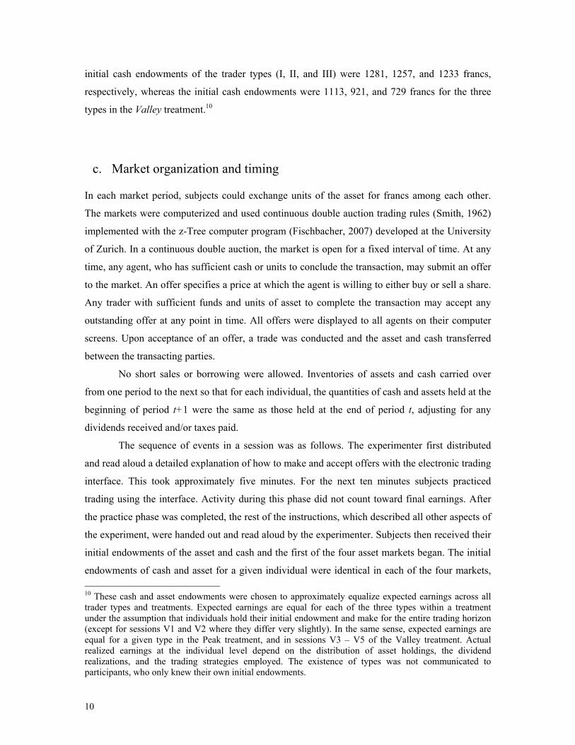
types in the Valley treatment.10

c. Market organization and timing

In each market period, subjects could exchange units of the asset for francs among each other.

The markets were computerized and used continuous double auction trading rules (Smith, 1962)

implemented with the z-Tree computer program (Fischbacher, 2007) developed at the University

of Zurich. In a continuous double auction, the market is open for a fixed interval of time. At any

time, any agent, who has sufficient cash or units to conclude the transaction, may submit an offer

to the market. An offer specifies a price at which the agent is willing to either buy or sell a share.

Any trader with sufficient funds and units of asset to complete the transaction may accept any

outstanding offer at any point in time. All offers were displayed to all agents on their computer

screens. Upon acceptance of an offer, a trade was conducted and the asset and cash transferred

between the transacting parties.

No short sales or borrowing were allowed. Inventories of assets and cash carried over

from one period to the next so that for each individual, the quantities of cash and assets held at the

beginning of period t+1 were the same as those held at the end of period t, adjusting for any

dividends received and/or taxes paid.

The sequence of events in a session was as follows. The experimenter first distributed

and read aloud a detailed explanation of how to make and accept offers with the electronic trading

interface. This took approximately five minutes. For the next ten minutes subjects practiced

trading using the interface. Activity during this phase did not count toward final earnings. After

the practice phase was completed, the rest of the instructions, which described all other aspects of

the experiment, were handed out and read aloud by the experimenter. Subjects then received their

initial endowments of the asset and cash and the first of the four asset markets began. The initial

endowments of cash and asset for a given individual were identical in each of the four markets, 10 These cash and asset endowments were chosen to approximately equalize expected earnings across all trader types and treatments. Expected earnings are equal for each of the three types within a treatment under the assumption that individuals hold their initial endowment and make for the entire trading horizon (except for sessions V1 and V2 where they differ very slightly). In the same sense, expected earnings are equal for a given type in the Peak treatment, and in sessions V3 – V5 of the Valley treatment. Actual realized earnings at the individual level depend on the distribution of asset holdings, the dividend realizations, and the trading strategies employed. The existence of types was not communicated to participants, who only knew their own initial endowments.

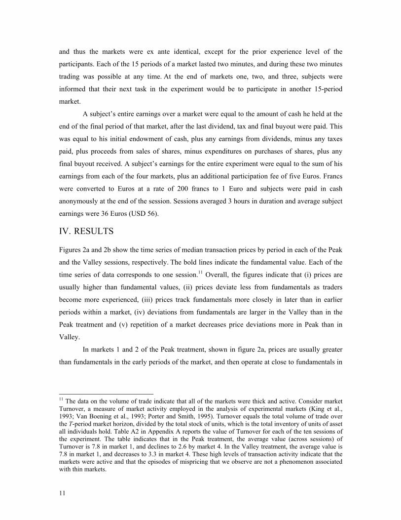
11

and thus the markets were ex ante identical, except for the prior experience level of the

participants. Each of the 15 periods of a market lasted two minutes, and during these two minutes

trading was possible at any time. At the end of markets one, two, and three, subjects were

informed that their next task in the experiment would be to participate in another 15-period

market.

A subject’s entire earnings over a market were equal to the amount of cash he held at the

end of the final period of that market, after the last dividend, tax and final buyout were paid. This

was equal to his initial endowment of cash, plus any earnings from dividends, minus any taxes

paid, plus proceeds from sales of shares, minus expenditures on purchases of shares, plus any

final buyout received. A subject’s earnings for the entire experiment were equal to the sum of his

earnings from each of the four markets, plus an additional participation fee of five Euros. Francs

were converted to Euros at a rate of 200 francs to 1 Euro and subjects were paid in cash

anonymously at the end of the session. Sessions averaged 3 hours in duration and average subject

earnings were 36 Euros (USD 56).

IV. RESULTS

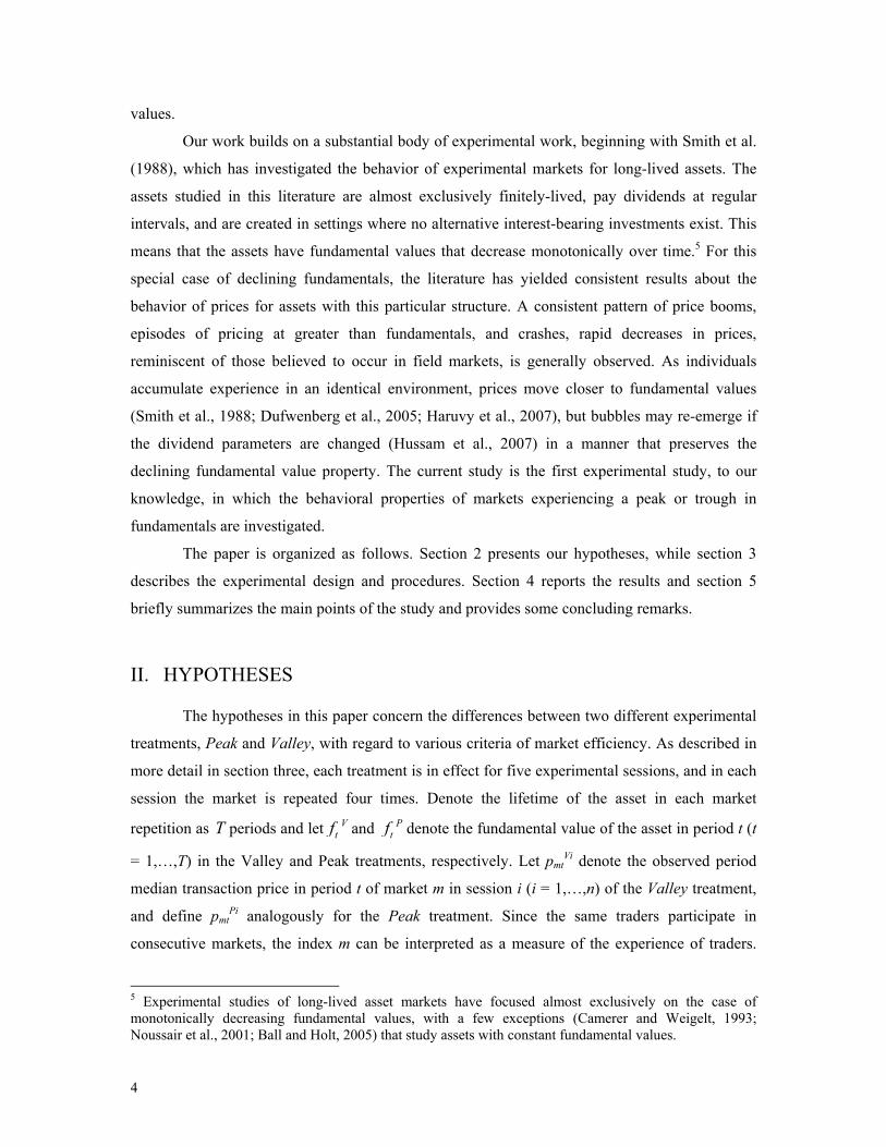
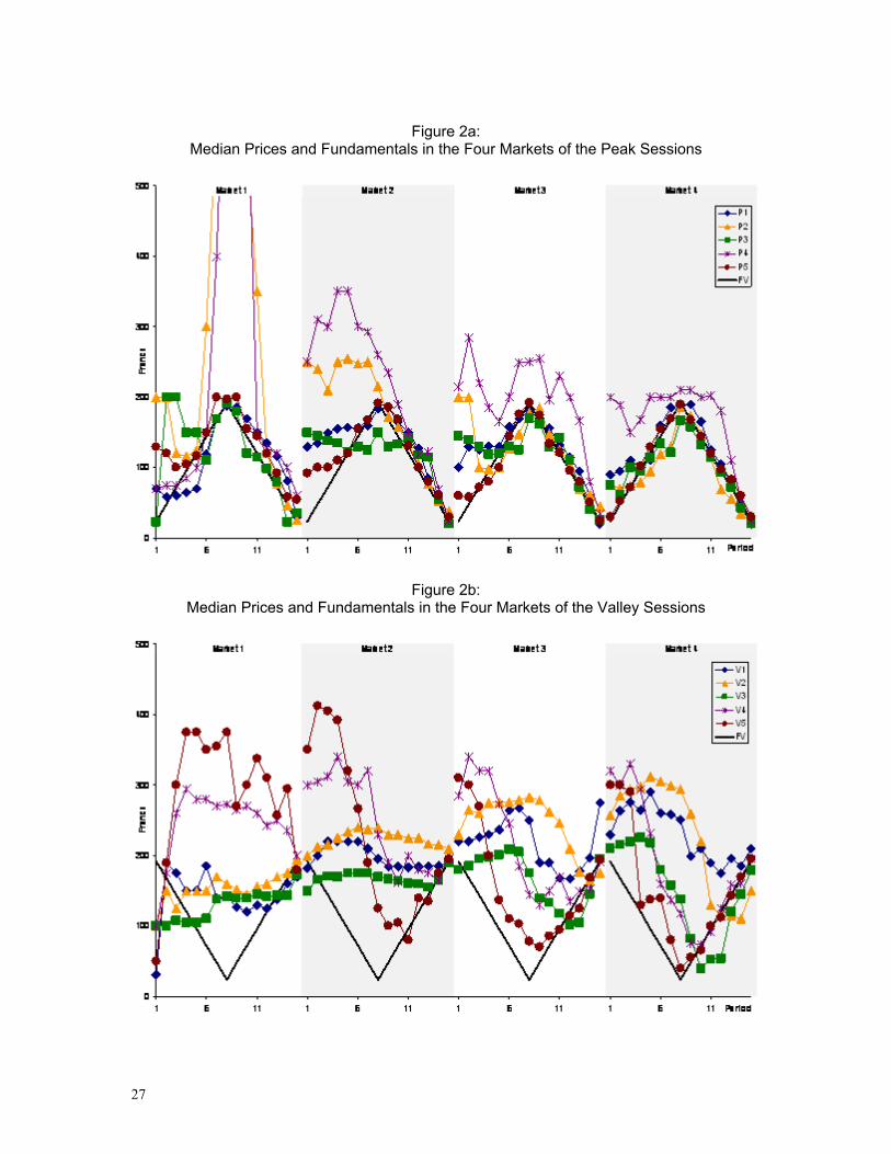
Figures 2a and 2b show the time series of median transaction prices by period in each of the Peak

and the Valley sessions, respectively. The bold lines indicate the fundamental value. Each of the

time series of data corresponds to one session.11 Overall, the figures indicate that (i) prices are

usually higher than fundamental values, (ii) prices deviate less from fundamentals as traders

become more experienced, (iii) prices track fundamentals more closely in later than in earlier

periods within a market, (iv) deviations from fundamentals are larger in the Valley than in the

Peak treatment and (v) repetition of a market decreases price deviations more in Peak than in

Valley.

In markets 1 and 2 of the Peak treatment, shown in figure 2a, prices are usually greater

than fundamentals in the early periods of the market, and then operate at close to fundamentals in

11 The data on the volume of trade indicate that all of the markets were thick and active. Consider market Turnover, a measure of market activity employed in the analysis of experimental markets (King et al., 1993; Van Boening et al., 1993; Porter and Smith, 1995). Turnover equals the total volume of trade over the T-period market horizon, divided by the total stock of units, which is the total inventory of units of asset all individuals hold. Table A2 in Appendix A reports the value of Turnover for each of the ten sessions of the experiment. The table indicates that in the Peak treatment, the average value (across sessions) of Turnover is 7.8 in market 1, and declines to 2.6 by market 4. In the Valley treatment, the average value is 7.8 in market 1, and decreases to 3.3 in market 4. These high levels of transaction activity indicate that the markets were active and that the episodes of mispricing that we observe are not a phenomenon associated with thin markets.

12

the latter periods. Sessions 2 and 4 experience particularly large booms12. By market 4, prices

track fundamentals closely in four of the five Peak sessions. In the Valley treatment, shown in

figure 2b, prices begin substantially below fundamental value in market 1. The prices then

typically exhibit booms relative to fundamentals, increasing to levels well above fundamentals by

the middle of the market and remaining above fundamentals for the remainder of the market. In

subsequent markets, prices exceed fundamentals throughout the life of the asset. Late in markets

3 and 4, prices tend to crash to near fundamentals, which they then track for the remainder of the

market. However, in those markets of the Valley treatment exhibiting a price trough and rebound,

the time of the turnaround in prices is typically later than the turning point of fundamentals.

Overall, the figures suggest that prices track fundamental values better in the Peak than in the

Valley treatment. Result 1 reports the findings of our analysis of relative price level efficiency in

two treatments.

[Figures 2a and 2b: About Here]

Result 1: Price levels in Peak sessions are closer to fundamentals than they are in Valley

sessions. That is, price level inefficiency is greater in the Valley than in the Peak treatment.

Hypothesis 1 is rejected.

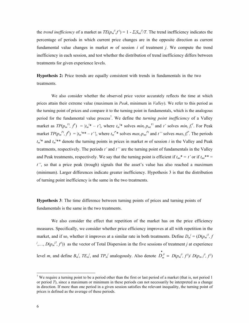
Support for Result 1: Figure 3 displays the observed values of Total Dispersion and Total Bias

in the two treatments, averaged across the five sessions within each treatment13. Recall that values

of Total Dispersion and of Total Bias closer to zero indicate lower price level inefficiency. In

figure 3, the measures are normalized by the value of the measure in market 1 of the Peak

treatment. The results show that mispricing in Valleys is consistently greater than in Peaks by

markets 3 and 4.

[Figure 3: About Here]

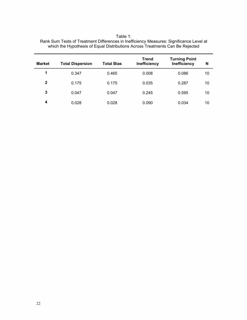
Table 1 indicates the results of two-sided rank-sum tests of differences in Total

Dispersion and Total Bias between the two treatments. The test is conducted separately for the

data from each of the four markets, which correspond to four different trader experience levels.

12 To avoid rescaling of the figures, the prices of some periods in market 1 of sessions P2 and P4 are not shown. These prices are 600, 800, and 600 in periods 7 – 9 of market 1 of P2, and 800, 750, and 700 in periods 8 – 10 of market 1 of P4. 13 The values of each measure for each market in each session of the Peak and Valley treatments are given in table A1 in the appendix. The table also reports the values of trend and turning point inefficiency for each market and session.

13

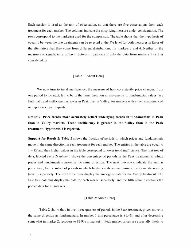
Each session is used as the unit of observation, so that there are five observations from each

treatment for each market. The columns indicate the mispricing measure under consideration. The

rows correspond to the market(s) used for the comparison. The table shows that the hypothesis of

equality between the two treatments can be rejected at the 5% level for both measures in favor of

the alternative that they come from different distributions, for markets 3 and 4. Neither of the

measures is significantly different between treatments if only the data from markets 1 or 2 is

considered. □

[Table 1: About Here]

We now turn to trend inefficiency, the measure of how consistently price changes, from

one period to the next, fail to be in the same direction as movements in fundamental values. We

find that trend inefficiency is lower in Peak than in Valley, for markets with either inexperienced

or experienced participants.

Result 2: Price trends more accurately reflect underlying trends in fundamentals in Peak

than in Valley markets. Trend inefficiency is greater in the Valley than in the Peak

treatment. Hypothesis 2 is rejected.

Support for Result 2: Table 2 shows the fraction of periods in which prices and fundamentals

move in the same direction in each treatment for each market. The entries in the table are equal to

1 – TE and thus higher values in the table correspond to lower trend inefficiency. The first row of

data, labeled Peak Treatment, shows the percentage of periods in the Peak treatment, in which

prices and fundamentals move in the same direction. The next two rows indicate the similar

percentage, for the subset of periods in which fundamentals are increasing (row 2) and decreasing

(row 3) separately. The next three rows display the analogous data for the Valley treatment. The

first four columns display the data for each market separately, and the fifth column contains the

pooled data for all markets.

[Table 2: About Here]

Table 2 shows that, in over three quarters of periods in the Peak treatment, prices move in

the same direction as fundamentals. In market 1 this percentage is 81.4%, and after decreasing

somewhat in market 2, recovers to 82.9% in market 4. Peak market prices are especially likely to

14

follow the same trend as fundamentals when fundamentals are decreasing (90.7% of periods) in

the later periods of the markets. In the Valley treatment, price movements are in the same

direction as fundamental changes in fewer than half of the periods in markets one and two, and

reach a level of consistency of greater than 60% only by market 4. No systematic difference in the

level of trend inefficiency is observed between periods in which fundamentals are increasing

versus when they are decreasing. Table 1 indicates the results of the test of the hypothesis that the

distribution of Trend Inefficiency is the same across treatments (as indicated previously, each

session is used as the unit of observation). The hypothesis is rejected in markets 1 and 2 at the 5%

level, and in market 4 at the 10% level. □

We now turn to turning point inefficiency, the relationship between the timing of the

turning point of fundamentals and the turning point in prices. Our observations are summarized

below as Result 3.

Result 3: Turning point inefficiency is greater in the Valley than in the Peak treatment.

Hypothesis 3 is rejected. By market 4 in the Peak treatment, the average turning point of

prices in the Peak treatment is very close to that of fundamentals. In the Valley treatment,

the turning point of prices is consistently later than that of fundamentals.

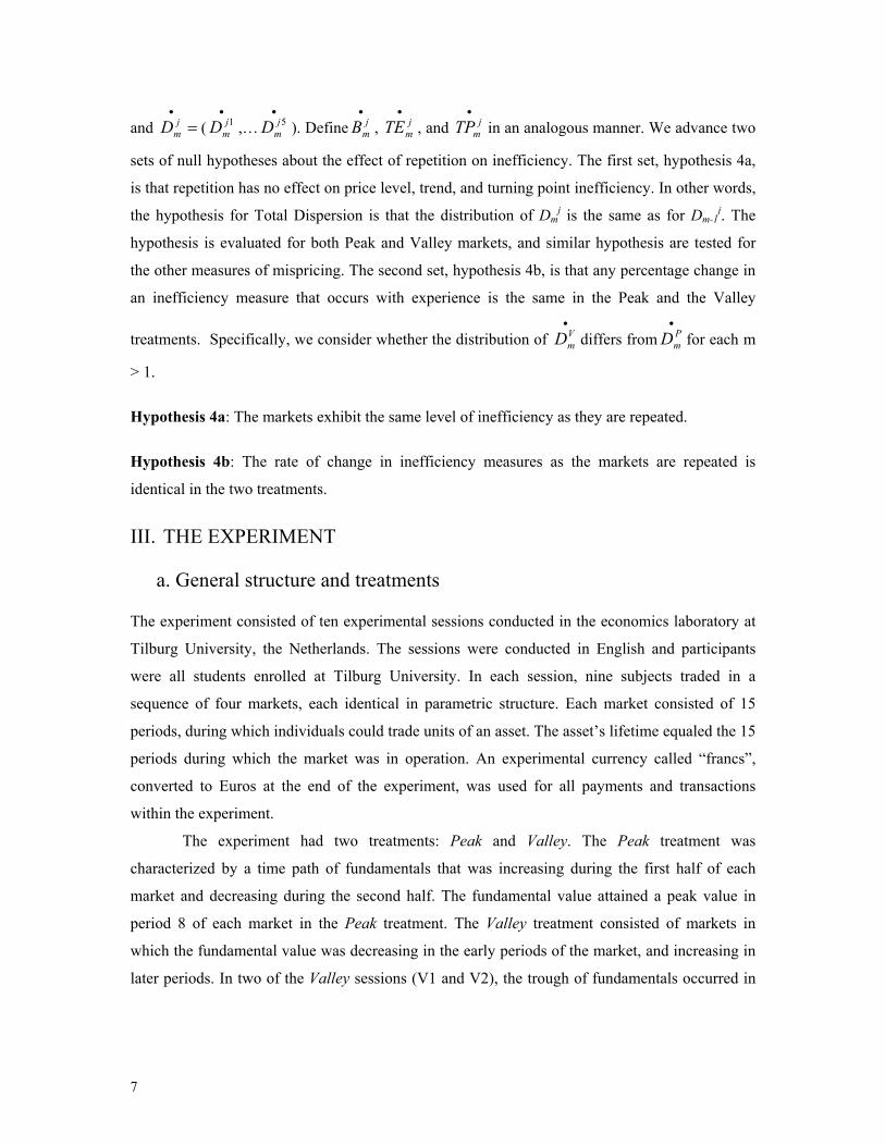
Support for Result 3: Figure 4 shows the difference between the turning points in prices and in

fundamentals by market in each session. Positive values on the horizontal axis indicate that prices

change direction later than fundamentals. The vertical axis indicates the number of sessions (out

of a total of five) that the difference between the two turning points equals the value of the

horizontal axis for the market shown in the panel. The turning points of prices are on average

earlier than those for fundamentals in the Peak treatment in markets 1 – 3, but the difference is

close to zero by market 4. The average turning point of prices in Valley is close to that of

fundamentals in market 1, although all but one of the actual turning points of prices is at least 4

periods away from the turning point of fundamentals. However, in Valley, after the first market,

price turning points are consistently later than those of fundamentals, and later than those in the

Peak treatment.

The fourth column of data in table 4 contains the significance levels of rank-sum tests of

the hypothesis that the distribution of Turning Point Inefficiency is equal between the two

treatments. The tests show that in market 4, the hypothesis of equality is rejected at the 5% level.

The hypothesis is rejected at the 10% level for market 1. □

15

[Figure 4: About Here]

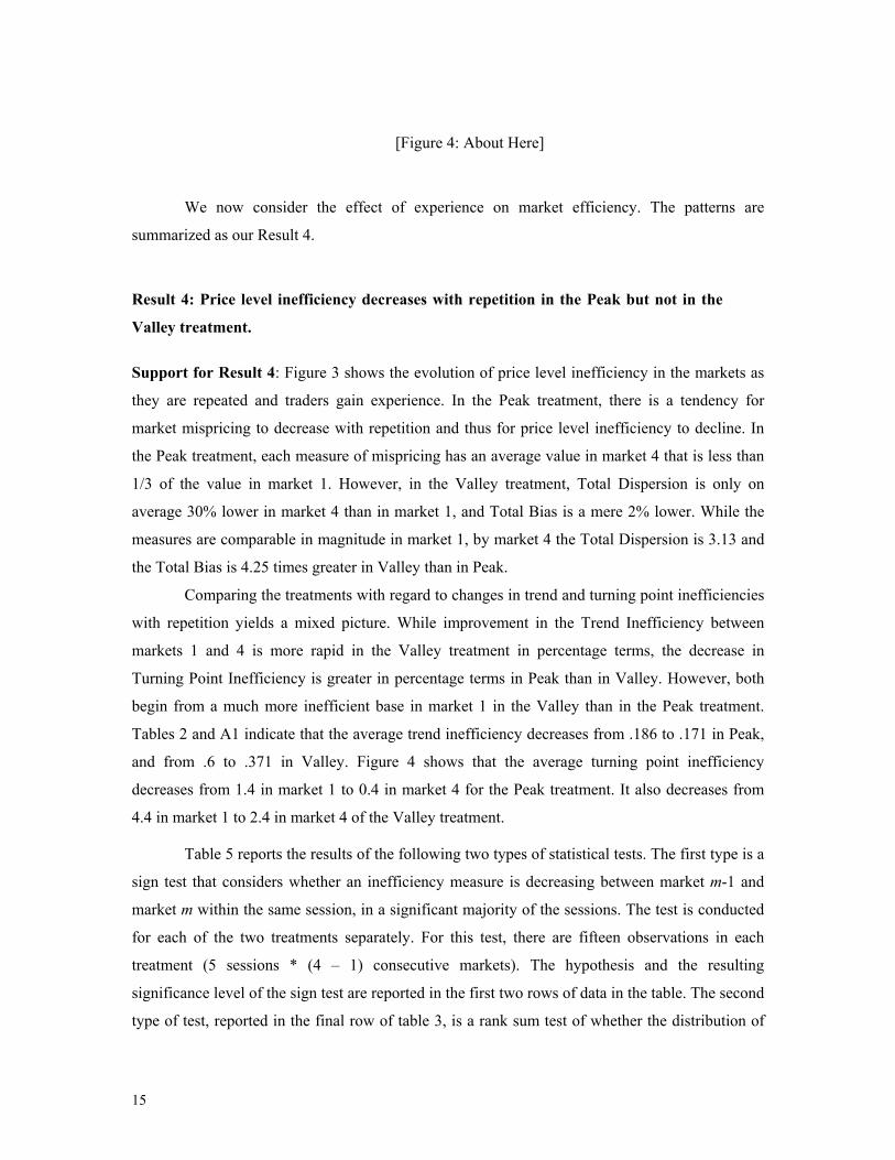
We now consider the effect of experience on market efficiency. The patterns are

summarized as our Result 4.

Result 4: Price level inefficiency decreases with repetition in the Peak but not in the

Valley treatment.

Support for Result 4: Figure 3 shows the evolution of price level inefficiency in the markets as

they are repeated and traders gain experience. In the Peak treatment, there is a tendency for

market mispricing to decrease with repetition and thus for price level inefficiency to decline. In

the Peak treatment, each measure of mispricing has an average value in market 4 that is less than

1/3 of the value in market 1. However, in the Valley treatment, Total Dispersion is only on

average 30% lower in market 4 than in market 1, and Total Bias is a mere 2% lower. While the

measures are comparable in magnitude in market 1, by market 4 the Total Dispersion is 3.13 and

the Total Bias is 4.25 times greater in Valley than in Peak.

Comparing the treatments with regard to changes in trend and turning point inefficiencies

with repetition yields a mixed picture. While improvement in the Trend Inefficiency between

markets 1 and 4 is more rapid in the Valley treatment in percentage terms, the decrease in

Turning Point Inefficiency is greater in percentage terms in Peak than in Valley. However, both

begin from a much more inefficient base in market 1 in the Valley than in the Peak treatment.

Tables 2 and A1 indicate that the average trend inefficiency decreases from .186 to .171 in Peak,

and from .6 to .371 in Valley. Figure 4 shows that the average turning point inefficiency

decreases from 1.4 in market 1 to 0.4 in market 4 for the Peak treatment. It also decreases from

4.4 in market 1 to 2.4 in market 4 of the Valley treatment.

Table 5 reports the results of the following two types of statistical tests. The first type is a

sign test that considers whether an inefficiency measure is decreasing between market m-1 and

market m within the same session, in a significant majority of the sessions. The test is conducted

for each of the two treatments separately. For this test, there are fifteen observations in each

treatment (5 sessions * (4 – 1) consecutive markets). The hypothesis and the resulting

significance level of the sign test are reported in the first two rows of data in the table. The second

type of test, reported in the final row of table 3, is a rank sum test of whether the distribution of

16

percentage changes in an inefficiency measure from one market to the next is significantly

different between the two treatments.

The table indicates, in the first two rows of data, the levels of significance at which we

can reject the null hypotheses that an inefficiency measure is the same or increasing between

market m-1 and m within the sessions. The first row shows that for the Peak treatment, the null

hypothesis is rejected for both Total Dispersion and Total Bias at the 5% level. For Valley, the

same hypotheses cannot be rejected, indicating that there is no significant decrease in the values

of these measures with repetition. We do reject the hypothesis, for the Valley data, that Trend

Inefficiency is constant or increasing from one market to the next in favor of the hypothesis that it

is decreasing. However, recall that the Trend Inefficiency levels in the Valley treatment in

markets one and two are greater than 50%, the value that would result if price movements were

purely random, so the improvement occurs from a very low base.

[Table 3: About Here]

The last row of the table indicates the significance level of a rank-sum test of the

hypothesis that the magnitude of percentage changes in an inefficiency measure from one market

to the next is equal between the two treatments. Significant values indicate rejection of the

hypothesis of equality. The data show that the improvement in price level inefficiency is

significantly different between Peak and Valley by both measures at p < .025. The improvement

is also greater for turning point inefficiency at the p < .1 level of significance. □

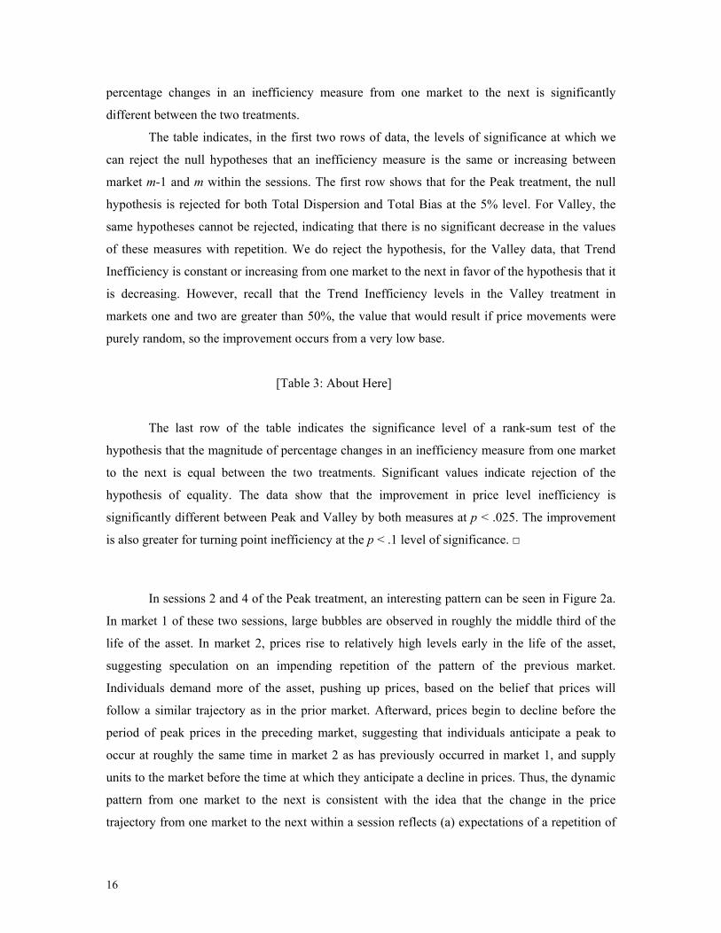
In sessions 2 and 4 of the Peak treatment, an interesting pattern can be seen in Figure 2a.

In market 1 of these two sessions, large bubbles are observed in roughly the middle third of the

life of the asset. In market 2, prices rise to relatively high levels early in the life of the asset,

suggesting speculation on an impending repetition of the pattern of the previous market.

Individuals demand more of the asset, pushing up prices, based on the belief that prices will

follow a similar trajectory as in the prior market. Afterward, prices begin to decline before the

period of peak prices in the preceding market, suggesting that individuals anticipate a peak to

occur at roughly the same time in market 2 as has previously occurred in market 1, and supply

units to the market before the time at which they anticipate a decline in prices. Thus, the dynamic

pattern from one market to the next is consistent with the idea that the change in the price

trajectory from one market to the next within a session reflects (a) expectations of a repetition of

17

the price time series that occurred in the prior market, in conjunction with (b) the use of profitable

strategies given those expectations.14

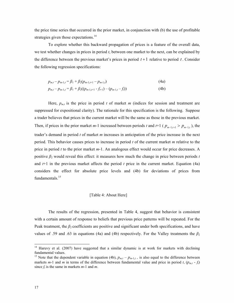
To explore whether this backward propagation of prices is a feature of the overall data,

we test whether changes in prices in period t, between one market to the next, can be explained by

the difference between the previous market’s prices in period 1t + relative to period t . Consider

the following regression specifications:

pm,t – pm-1,t = β1 + β2(pm-1,t+1 – pm-1,t) (4a)

pm,t – pm-1,t = β1 + β2((pm-1,t+1 - ft+1) – (pm-1,t – ft)) (4b)

Here, pm,t is the price in period t of market m (indices for session and treatment are

suppressed for expositional clarity). The rationale for this specification is the following. Suppose

a trader believes that prices in the current market will be the same as those in the previous market.

Then, if prices in the prior market m-1 increased between periods t and t+1 ( 1, 1 1,m t m tp p− + −> ), the

trader’s demand in period t of market m increases in anticipation of the price increase in the next

period. This behavior causes prices to increase in period t of the current market m relative to the

price in period t to the prior market m-1. An analogous effect would occur for price decreases. A

positive β2 would reveal this effect: it measures how much the change in price between periods t

and t+1 in the previous market affects the period t price in the current market. Equation (4a)

considers the effect for absolute price levels and (4b) for deviations of prices from

fundamentals.15

[Table 4: About Here]

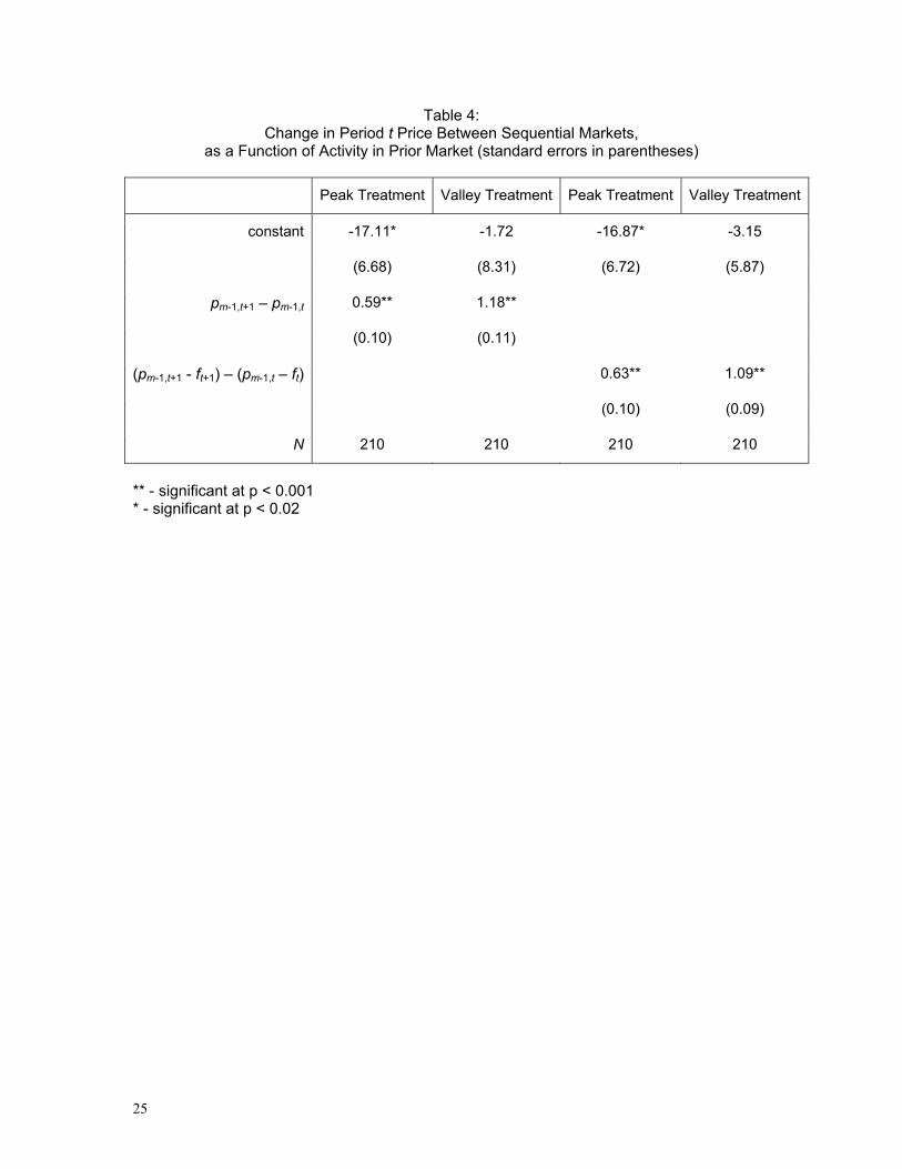
The results of the regression, presented in Table 4, suggest that behavior is consistent

with a certain amount of response to beliefs that previous price patterns will be repeated. For the

Peak treatment, the β2 coefficients are positive and significant under both specifications, and have

values of .59 and .63 in equations (4a) and (4b) respectively. For the Valley treatments the β2

14 Haruvy et al. (2007) have suggested that a similar dynamic is at work for markets with declining fundamental values. 15 Note that the dependent variable in equation (4b), pm,t – pm-1,t , is also equal to the difference between markets m-1 and m in terms of the difference between fundamental value and price in period t, (pm,t - ft) since ft is the same in markets m-1 and m.

18

coefficients are also positive and significant, with larger values in the Peak treatment, indicating

that the backward propagation of prices is even stronger in the Valley sessions.

V. CONCLUSION

We construct experimental markets to obtain the first empirical observations, from a controlled

laboratory study, of the behavior of asset markets that experience a peak or a trough in

fundamentals. We focus on how well the market tracks the fundamental value, how well it

reflects trends in fundamentals, and how well it reveals the timing of a change in trend. We also

consider how these measures of pricing accuracy evolve as traders gain more experience through

repetition of the market. The results are not obvious a priori in light of the strong tendency of

experimental asset markets to generate bubbles and crashes when traders are inexperienced, a

result that nonetheless has only been established for assets with fundamental values that are

monotonically decreasing or constant over time.

We observe that mispricing relative to fundamental values is typical in markets populated

with inexperienced subjects. As individuals gain experience, prices move much closer to

fundamental values in the Peak treatment, in a manner similar to that observed in previous studies

of experimental markets with declining fundamental values. However, in the time frame we are

able to observe, four repetitions of a 15-period market, the Valley treatment does not move

appreciably closer to fundamentals. Price changes from one period to the next are typically in the

same direction as the change in fundamentals in the Peak treatment, but not in the Valley

treatment. The observed peaks and troughs in prices accurately reflect the timing of the

turnaround in fundamental values in Peak, but are systematically too late in Valley.

Thus, we find a strong difference between the price efficiency of a market when the

underlying fundamentals rise to a peak and then decline, and that of a market where the

fundamentals decline to a trough and experience a subsequent increase. In the Peak treatment,

while the market experiences bubbles and crashes when traders are inexperienced, the markets

operate at close to fundamentals after participants have acquired experience in the environment.

On the other hand, a trough in fundamentals appears to represent a more challenging environment

for the market to achieve price efficiency. Prices consistently fail to reflect the level, the direction

of the trend, and the timing of the turnaround of fundamentals in the Valley treatment. The Valley

treatment is the first experimental environment of which we are aware, in which asset markets

populated by individuals with this level of experience with a stationary environment, do not track

fundamental values closely.

19

There is considerable debate in the economics profession about the extent to which

markets produce prices that reflect underlying fundamental values. The evidence we obtain here,

from ten experimental sessions, suggests that the answer may be that it depends on the properties

of the process underlying fundamental values and the dynamics the process exhibits over time.

We identify a strong asymmetry between how asset markets respond to peaks and troughs in

fundamentals. This occurs even though the treatments are constructed to be similar in the level of

complexity, in the monetary stakes involved, in the institutional structure, and in the

characteristics of the individuals participating. Indeed, there may also be characteristics of the

time path of fundamentals, other than whether they exhibit peaks and troughs, that enhance or

impede the ability of a market to track fundamentals. Our research indicates that characteristics of

the fundamental value, in addition to the well-known influences of the institutional structure and

the level of sophistication of traders, are determinants of price efficiency. While this is clearly a

property of the laboratory markets we study, it may also be a feature of markets outside the

laboratory. If so, it suggests a conjecture that the tendency of markets to conform more closely to

some trajectories of fundamentals than others might potentially reconcile differing conclusions on

the extent to which asset markets display price efficiency.

REFERENCES

Abreu, Dilip, and Markus K. Brunnermeier, 2003. “Bubbles and Crashes”, Econometrica, Vol. 71, No. 1. (January), pp.

173-204.

Ball, Sheryl B., and Charles A. Holt, 1998. “Classroom Games: Speculation and Bubbles in an Asset Market”, Journal

of Economic Perspectives, vol. 12(1), Winter, pages 207-18.

Brunnermeier, Markus K., and Christian Julliard, 2008. “Money Illusion and Housing Frenzies”, Review of Financial

Studies, forthcoming.

Camerer, Colin, and Keith Weigelt, 1993. “Convergence in Experimental Double Auctions for Stochastically Lived

Assets”, with K. Weigelt, in D. Friedman & J. Rust (Eds.), The Double Auction Market: Theories, Institutions

and Experimental Evaluations, Redwood City, CA: Addison-Wesley, 355-396.

De Long, J. Bradford; Andrei Shleifer; Lawrence H. Summers; Robert J. Waldmann, 1990. “Noise Trader Risk in

Financial Markets”, Journal of Political Economy, Vol. 98, No. 4. (August), pp. 703-738.

Dufwenberg, Martin, Tobias Lindqvist, and Evan Moore, 2005. “Bubbles and Experience: An Experiment”, The

American Economic Review, Volume 95, Number 5 (December), pp. 1731-1737.

Fama, Eugene F., 1998. “Market efficiency, long-term returns, and behavioral finance”, Journal of Financial

Economics, Volume 49, Issue 3, 1 September, Pages 283-306.

Fischbacher, U. 2007. “z-Tree: Zurich Toolbox for Ready-Made Economic Experiments”, Experimental Economics,

20

Volume 10, No. 2, pp. 171-178.

French, Kenneth R., and James M. Poterba, 1991. “Were Japanese stock prices too high?” Journal of Financial

Economics, Volume 29, Issue 2 (October), Pages 337-363.

Froot, Kenneth A., and Maurice Obstfeld, 1991. “Intrinsic Bubbles: The Case of Stock Prices”, American Economic

Review, vol. 81(5) (December), pages 1189-214.

Garber, P. M., 1990. “Famous First Bubbles”, Journal of Economic Perspectives, Vol. 4, No. 2, pp 35-54.

Haruvy, E.; Y. Lahav; C. N. Noussair, 2007. “Traders’ Expectations in Asset Markets: Experimental Evidence”,

American Economic Review, Volume 97(5) (December), pp. 1901-1920.

Haruvy, E., and C. N. Noussair, 2006. “The Effect of Short Selling on Bubbles and Crashes in Experimental Spot Asset

Markets”, Journal of Finance 61 (June), 1119-1157.

Hussam, R, D. Porter, and V. L. Smith, 2007. “Thar She Blows: Can Bubbles Be Rekindled With Experienced

Subjects?” Working paper, Chapman University.

King, Ronald L.; Vernon L. Smith; Mark V. van Boening; and Arlington W. Williams, 1993. “The Robustness of

Bubbles and Crashes in Experimental Markets”, in Nonlinear Dynamics and Evolutionary Economics, Richard

H. Day and Ping Chen, eds., Oxford Press.

LeRoy, Stephen F, 2004. “Rational Exuberance”, Journal of Economic Literature, vol. 42, no. 3 (Fall), pp. 783-804.

Lei, Vivian; Charles N. Noussair; Charles R. Plott, 2001. “Nonspeculative Bubbles in Experimental Asset Markets:

Lack of Common Knowledge of Rationality vs. Actual Irrationality”, Econometrica, Vol. 69, No. 4. (July), pp.

831-859.

Malkiel, Burton G. 2003. “The Efficient Market Hypothesis and Its Critics”, Journal of Economic Perspectives, vol.

17, no. 1 (Winter) pp 59-82.

Noussair, Charles, Stephane Robin and Bernard Ruffieux, 2001. “Price Bubbles in Laboratory Asset Markets with

Constant Fundamental Values”, Experimental Economics, vol. 4, June, pp 87-105.

Pastor, Lubos and Pietro Veronesi, 2006. “Was there a Nasdaq bubble in the late 1990s?” Journal of Financial

Economics, Volume 81, Issue 1, July, pp. 61-100.

Reshmaan, N. Hussam; Porter, David and Vernon L. Smith: “Thar' She Blows: Rekindling Bubbles with Experienced

Subjects”, American Economic Review, forthcoming.

Roll, Richard, 1988. “R^2”, Journal of Finance, Vol. 43, No. 3, pp. 541-566.

Scheinkman, Jose and Wei Xiong, 2003. “Overconfidence and Speculative Bubbles”, Journal of Political Economy,

(December), pp. 1183-1219.

Shiller, Robert J, 1981. “Do Stock Prices Move Too Much to be Justified by Subsequent Changes in Dividends?”,

American Economic Review, vol. 71, no. 3 (June), pp 421-436.

- , 2003, “From Efficient Markets Theory to Behavioral Finance”, The Journal of Economic Perspectives, Vol.

17, No. 1 (Winter), pp. 83-104.

Smith, Vernon L., 1962. “An Experimental Study of Competitive Market Behavior”, Journal of Political Economy,

21

Volume 70, No. 2, pp. 111-137.

Smith, Vernon L , Gerry L. Suchanek, and Arlington W. Williams, 1988. “Bubbles, Crashes, and Endogenous

Expectations in Experimental Spot Asset Markets”, Econometrica, vol. 56, no. 5 (September) pp. 1119-51.

Temin, Peter; Hans-Joachim Voth, 2004. “Riding the South Sea Bubble”, American Economic Review, Vol. 94, No. 5.

(December), pp. 1654-1668.

Tirole, Jean, 1982. “On the Possibility of Speculation under Rational Expectations”, Econometrica, Vol. 50, No. 5.

(September), pp. 1163-1181.

Van Boening, Mark V. & Williams, Arlington W. & LaMaster, Shawn, 1993. “Price bubbles and crashes in

experimental call markets”, Economics Letters, vol. 41(2), pages 179-185.

22

Table 1:

Rank Sum Tests of Treatment Differences in Inefficiency Measures: Significance Level at which the Hypothesis of Equal Distributions Across Treatments Can Be Rejected

Market Total Dispersion Total Bias Trend

Inefficiency Turning Point Inefficiency N

1 0.347 0.465 0.008 0.086 10

2 0.175 0.175 0.035 0.287 10

3 0.047 0.047 0.245 0.595 10

4 0.028 0.028 0.090 0.034 10

23

Table 2: Fraction of Periods in Which Price and Fundamental Value Movements

Are in the Same Direction, Overall, and for Periods with Decreasing and

Increasing Fundamentals Separately

Market 1 Market 2 Market 3 Market 4 All Markets

Peak Treatment .814 .729 .757 .829 .782

Peak Treatment, when ftP > ft-1P .686 .571 .629 .743 .657

Peak Treatment, when ftP < ft-1P .943 .886 .886 .914 .907

Valley Treatment .400 .414 .514 .629 .489

Valley Treatment, when ftV > ft-1V .515 .364 .545 .636 .515

Valley Treatment, when ftV < ft-1V .297 .459 .486 .622 .466

All Periods and Treatments .607 .571 .636 .729 .636

24

Table 3: Statistical Tests and Results of Hypotheses of No Change in Efficiency Measures

Between Consecutive Markets and of Similar Rates of Change Between Treatments

Hypothesis/Significance Level of test of Hypothesis

Total Dispersion Total Bias Trend Inefficiency

Turning Point Infficiency

N

Peak Treatment: Value of measure same or greater in market m than in m - 1

Significance Level of Test of Hypothesis

DmP =Dm-1

P .0037

BmP = Bm-1

P .0176

TEmP =TEm-1

P .5000

TPPm = TPP

m-1 .2539

15

Valley Treatment: Value of measure same or greater in market m than in m - 1

Significance Level of Test of Hypothesis

DmV(.)=Dm-1

V(.) .5000

BmV(.)=Bm-1

V(.) .5000

TEmV =TEm-1

V .0461

TPVm = TPV

m-1 .1334

15

Percent change of measure between market m – 1 to m the same in Peak and Valley

Significance Level of Test of Hypothesis

•VmD =

•PmD

.0095

•VmB =

•PmB

.0238

•VmTE =

•PmTE

.1965

•V

mTP =•

PmTP

.0686

30

25

Table 4: Change in Period t Price Between Sequential Markets,

as a Function of Activity in Prior Market (standard errors in parentheses)

Peak Treatment Valley Treatment Peak Treatment Valley Treatment

constant -17.11* -1.72 -16.87* -3.15

(6.68) (8.31) (6.72) (5.87)

pm-1,t+1 – pm-1,t 0.59** 1.18**

(0.10) (0.11)

(pm-1,t+1 - ft+1) – (pm-1,t – ft) 0.63** 1.09**

(0.10) (0.09)

N 210 210 210 210

** - significant at p < 0.001 * - significant at p < 0.02

26

Figure 1: Time path of fundamentals in the two treatments,

(a) Peak and (b) Valley treatments.

0

200

400

1 15

Francs

DividendsTaxes

0

200

400

1 15Period

Final buyoutDividends

Taxes Period

Francs

P1 – P5 V1 – V2

V3 – V5

(a) Peak treatment. (b) Valley treatment.

27

Figure 2a:

Median Prices and Fundamentals in the Four Markets of the Peak Sessions

Figure 2b: Median Prices and Fundamentals in the Four Markets of the Valley Sessions

28

Figure 3: Price Level Inefficiency Measures in Peak (dark bars) and Valley (light bars),

Averaged over Sessions (Value in Peak-Market 1 = 1.0)

Total Dispersion Total Bias

0.0

0.4

0.8

1.2

1.6

1 2 3 40.0

0.4

0.8

1.2

1.6

1 2 3 4 Market Market

29

Figure 4: Differences Between Turning Point of Prices and Turning Point of

Fundamentals by Session, Both Treatments and Each of the Four Markets

Market

Peak Treatment Valley Treatment

1

0

1

2

3

-6 -5 -4 -3 -2 -1 0 1 2 3 4 5 6 0

1

2

3

-6 -5 -4 -3 -2 -1 0 1 2 3 4 5 6

2

0

1

2

3

-6 -5 -4 -3 -2 -1 0 1 2 3 4 5 6 0

1

2

3

-6 -5 -4 -3 -2 -1 0 1 2 3 4 5 6

3

0

1

2

3

-6 -5 -4 -3 -2 -1 0 1 2 3 4 5 6 0

1

2

3

-6 -5 -4 -3 -2 -1 0 1 2 3 4 5 6

4 0

1

2

3

-6 -5 -4 -3 -2 -1 0 1 2 3 4 5 6 t’’ – t**

0

1

2

3

-6 -5 -4 -3 -2 -1 0 1 2 3 4 5 6 t’ – t*

30

Appendix A: Supplementary Data and Statistical Tests

This appendix contains three tables. The first table, A1, displays the values of the four

measures of price efficiency (Total Dispersion, Total Bias, Trend Inefficiency, and Turning Point

Difference) in each market of each session. The table also includes the averages across sessions

within each treatment, and the between-session standard deviations.

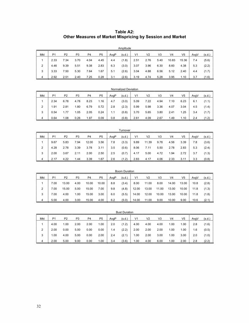
The second table, A2, shows the values for several measures of market bubbles that

previous authors (King et al., 1993; Porter and Smith, 1995; Haruvy and Noussair, 2006) have

employed. These measures are:

(1) Amplitude = ( ) ( )tmax min/ /tt t t tt tP f P ff f−− − , where tP and tf equal the median

transaction price and fundamental value in period t , respectively.

(2) Normalized Deviation = ( )/ 100it ti tP f TSU− ⋅∑ ∑ , where itP is the price of the ith

transaction in period t. TSU is the total stock of units that agents hold.

(3) Turnover = /ttq TSU∑ , where tq is the quantity of units of the asset exchanged in

period t.

(4) Boom Duration = the greatest number of consecutive periods median transaction prices

are above fundamental values.

(5) Bust Duration = the greatest number of consecutive periods median transaction prices

are below fundamental values.

In the table, the measures are reported for each market within each session. The table also

includes averages across sessions for each treatment, as well as between session standard

deviations.

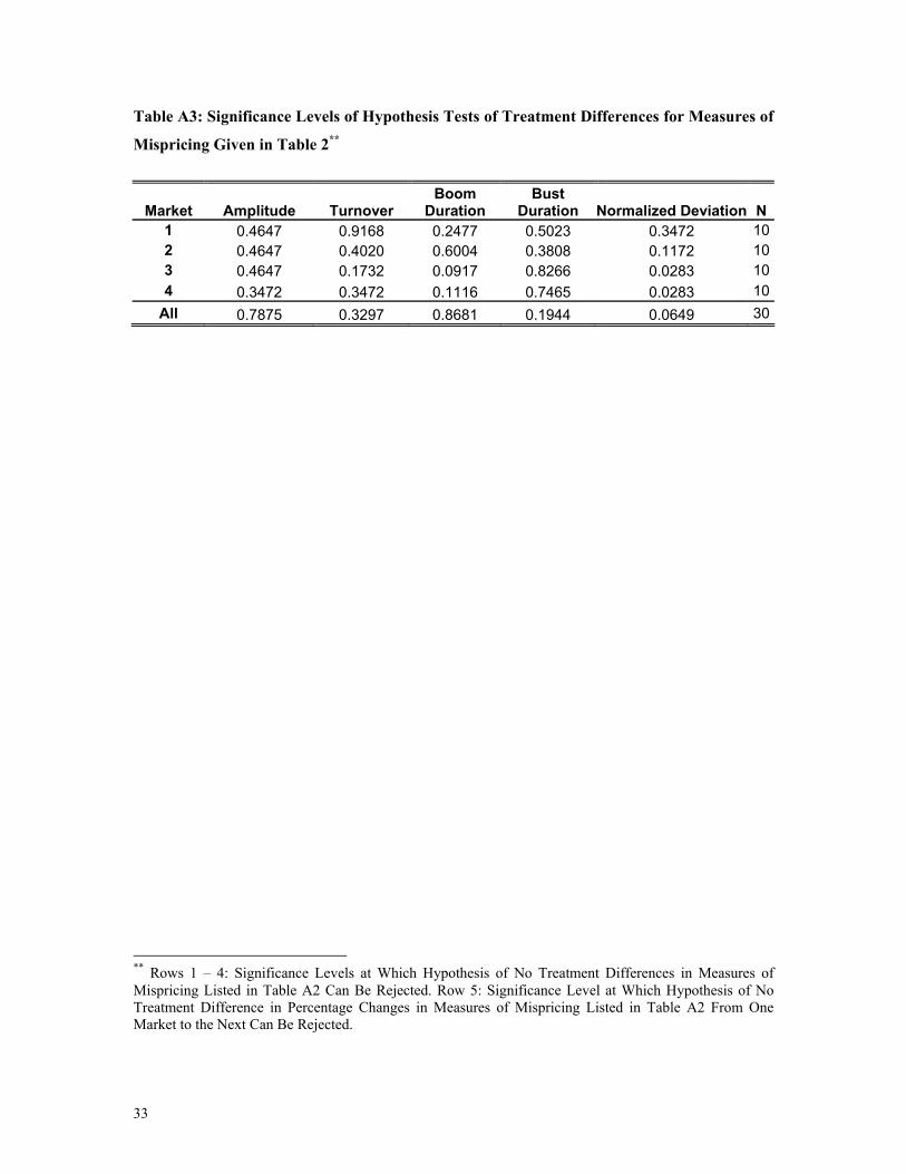
Finally, Table A3 contains the results of an analysis of the differences between treatments

of each of the measures defined above. The tables report, for each measure and in each market,

the significance level at which the hypothesis that the values for both treatments are drawn from

the same population can be rejected.

31

Table A1: Measures of Mispricing by Session and Market

Total Dispersion

Mkt P1 P2 P3 P4 P5 AvgP (s.d.) V1 V2 V3 V4 V5 AvgV (s.d.)

1 375.50 2697.00 489.00 2289.50 414.50 1253.1 (1142.0) 658.50 801.50 742.00 2135.00 2924.00 1452.2 (1023.5)

2 519.50 1118.50 576.50 1786.50 258.00 851.8 (609.0) 1025.50 1352.00 907.50 1982.00 1736.00 1400.6 (457.4)

3 368.50 499.50 438.50 1394.50 118.50 563.9 (486.4) 1230.50 1628.00 967.00 1519.00 708.00 1210.5 (381.3)

4 275.50 260.00 220.50 965.00 74.00 359.0 (348.0) 1391.50 1622.50 937.50 1089.00 584.50 1125.0 (402.2)

Total Bias

Mkt P1 P2 P3 P4 P5 AvgP (s.d.) V1 V2 V3 V4 V5 AvgV (s.d.)

1 130.50 2694.00 310.05 2225.55 407.55 1153.5 1208.0 45.45 219.45 229.05 1951.05 2616.00 1012.5 1186.4

2 485.55 1118.55 272.55 1786.50 258.00 784.5 660.4 874.50 1264.95 809.55 1975.95 1686.00 1321.5 506.5

3 336.45 353.55 225.45 1394.55 27.45 468.0 534.3 1190.55 1569.00 781.05 1486.95 658.05 1137.0 408.7

4 232.50 -88.05 -32.55 964.95 70.05 229.5 428.9 1371.45 1355.55 530.55 1063.05 555.45 975.0 413.3

Trend Inefficiency (Proportion of Periods with Opposite Trend in Fundamentals and Prices)

Mkt P1 P2 P3 P4 P5 AvgP (s.d.) V1 V2 V3 V4 V5 AvgV (s.d.)

1 0.07 0.14 0.36 0.07 0.29 0.19 (0.1) 0.43 0.43 0.71 0.71 0.71 0.60 (0.2)

2 0.07 0.29 0.50 0.43 0.07 0.27 (0.2) 0.57 0.79 0.64 0.64 0.29 0.59 (0.2)

3 0.14 0.29 0.36 0.36 0.07 0.24 (0.1) 0.64 0.79 0.64 0.29 0.07 0.49 (0.3)

4 0.14 0.07 0.21 0.43 0.00 0.17 (0.2) 0.43 0.64 0.36 0.21 0.21 0.37 (0.2)

Turning Point Difference

Mkt P1 P2 P3 P4 P5 AvgP (s.d.) V1 V2 V3 V4 V5 AvgV (s.d.)

1 0.00 0.00 6.00 0.00 1.00 1.4 (2.6) 8.00 8.00 7.00 7.00 7.00 7.4 (0.5)

2 1.00 3.00 7.00 4.00 0.00 3.0 (2.7) 8.00 8.00 7.00 2.00 3.00 5.6 (2.9)

3 0.00 7.00 0.00 6.00 0.00 2.6 (3.6) 3.00 5.00 4.00 1.00 1.00 2.8 (1.8)

4 1.00 0.00 0.00 0.00 0.00 0.2 (0.4) 3.00 5.00 2.00 2.00 0.00 2.4 (1.8)

32

Table A2: Other Measures of Market Mispricing by Session and Market

Amplitude

Mkt P1 P2 P3 P4 P5 AvgP (s.d.) V1 V2 V3 V4 V5 AvgV (s.d.)

1 2.33 7.34 3.70 4.04 4.45 4.4 (1.8) 2.51 2.76 5.40 10.83 15.36 7.4 (5.6)

2 4.46 9.39 5.51 9.38 2.83 6.3 (3.0) 3.07 3.96 6.30 8.60 4.38 5.3 (2.2)

3 3.33 7.50 5.30 7.64 1.67 5.1 (2.6) 3.04 4.88 6.56 5.12 2.40 4.4 (1.7)

4 2.92 2.51 2.40 7.25 0.28 3.1 (2.6) 3.19 4.74 5.28 3.95 1.10 3.7 (1.6)

Normalized Deviation

Mkt P1 P2 P3 P4 P5 AvgP (s.d.) V1 V2 V3 V4 V5 AvgV (s.d.)

1 2.34 6.78 4.78 8.23 1.16 4.7 (3.0) 5.09 7.22 4.94 7.10 6.23 6.1 (1.1)

2 1.91 2.81 1.80 6.79 0.72 2.8 (2.3) 5.99 5.98 3.36 4.07 3.04 4.5 (1.4)

3 0.54 1.77 1.05 2.05 0.24 1.1 (0.8) 3.70 5.65 3.80 2.41 1.25 3.4 (1.7)

4 0.64 1.08 0.26 1.97 0.09 0.8 (0.8) 2.61 4.09 2.67 1.49 1.10 2.4 (1.2)

Turnover

Mkt P1 P2 P3 P4 P5 AvgP (s.d.) V1 V2 V3 V4 V5 AvgV (s.d.)

1 9.67 5.83 7.94 12.00 3.56 7.8 (3.3) 9.89 11.39 9.78 4.56 3.39 7.8 (3.6)

2 4.28 2.78 3.39 3.78 3.11 3.5 (0.6) 8.06 7.11 5.50 2.78 2.83 5.3 (2.4)

3 2.00 3.67 2.11 2.00 2.50 2.5 (0.7) 4.17 5.00 4.72 1.94 2.72 3.7 (1.3)

4 2.17 4.22 1.44 3.39 1.67 2.6 (1.2) 2.83 4.17 4.06 2.33 3.11 3.3 (0.8)

Boom Duration

Mkt P1 P2 P3 P4 P5 AvgP (s.d.) V1 V2 V3 V4 V5 AvgV (s.d.)

1 7.00 13.00 4.00 10.00 10.00 8.8 (3.4) 8.00 11.00 8.00 14.00 13.00 10.8 (2.8)

2 7.00 15.00 5.00 15.00 7.00 9.8 (4.8) 12.00 13.00 11.00 13.00 10.00 11.8 (1.3)

3 7.00 4.00 1.00 15.00 3.00 6.0 (5.5) 14.00 12.00 10.00 13.00 10.00 11.8 (1.8)

4 5.00 4.00 3.00 15.00 4.00 6.2 (5.0) 14.00 11.00 9.00 10.00 9.00 10.6 (2.1)

Bust Duration

Mkt P1 P2 P3 P4 P5 AvgP (s.d.) V1 V2 V3 V4 V5 AvgV (s.d.)

1 4.00 1.00 2.00 2.00 1.00 2.0 (1.2) 4.00 4.00 4.00 1.00 1.00 2.8 (1.6)

2 2.00 0.00 5.00 0.00 0.00 1.4 (2.2) 2.00 2.00 2.00 1.00 1.00 1.6 (0.5)

3 1.00 4.00 5.00 0.00 2.00 2.4 (2.1) 1.00 2.00 3.00 1.00 3.00 2.0 (1.0)

4 2.00 5.00 9.00 0.00 1.00 3.4 (3.6) 1.00 4.00 6.00 1.00 2.00 2.8 (2.2)

33

Table A3: Significance Levels of Hypothesis Tests of Treatment Differences for Measures of

Mispricing Given in Table 2**

Market Amplitude Turnover Boom

Duration Bust

Duration Normalized Deviation N1 0.4647 0.9168 0.2477 0.5023 0.3472 102 0.4647 0.4020 0.6004 0.3808 0.1172 103 0.4647 0.1732 0.0917 0.8266 0.0283 104 0.3472 0.3472 0.1116 0.7465 0.0283 10

All 0.7875 0.3297 0.8681 0.1944 0.0649 30

** Rows 1 – 4: Significance Levels at Which Hypothesis of No Treatment Differences in Measures of Mispricing Listed in Table A2 Can Be Rejected. Row 5: Significance Level at Which Hypothesis of No Treatment Difference in Percentage Changes in Measures of Mispricing Listed in Table A2 From One Market to the Next Can Be Rejected.

34

Appendix B: Experiment Instructions and Screen Displays

This appendix contains the instructions handed out to subjects and two screenshots of the trading program in action. Treatment-specific information is contained inside curly braces { } for the Peak treatment and square brackets [ ] for sessions V3-V5 of the Valley treatment (information for V1-V2 is omitted, as it is very similar to the information in V3-V5). --- BEGIN INSTRUCTIONS --- 1. General Instructions This is an experiment on decision making in a market. The instructions are simple and if you follow them carefully and make good decisions, you might earn a considerable amount of money, which will be paid to you in cash at the end of the experiment. The experiment consists of a sequence of trading Periods in which you will have the opportunity to buy and sell in a market. The currency used in the market is francs. All trading will be done in terms of francs. The cash payment to you at the end of the experiment will be in Euros. The conversion rate is: 200 francs to 1 Euro. 2. How to use the computerized market In the top right hand corner of the screen you see how much time is left in the current Period. The goods that can be bought and sold in the market are called Shares. In the center of your screen you see the current Period and the amount of Money you have available to buy Shares. To the left of the screen, you see the number of Shares you currently have. If you would like to offer to sell a share, use the text area entitled “Enter offer to sell:” in the second column. In that text area you can enter the price at which you are offering to sell a share, and then select “Submit Offer To Sell”. Please do so now. Type in a number in the appropriate space, and then click on the field labelled “Submit Offer To Sell”. You will notice that nine numbers, one submitted by each participant, now appear in the third column from the left, entitled “Offers To Sell”. The lowest ask price will always be on the bottom of that list and will, by default, be selected. You can select a different offer by clicking on it. If you select “Buy”, the button at the bottom of this column, you will buy one share for the currently selected sell price. Please purchase a share now by selecting “Buy”. Since each of you had offered to sell a share and attempted to buy a share, if all were successful, you all have the same number of shares you started out with. This is because you bought one share and sold one share. When you buy a share, your Money decreases by the price of the purchase. When you sell a share, your Money increases by the price of the sale. You may make an offer to buy a unit by selecting “Submit offer to buy.” Please do so now. Type a number in the text area “Enter offer to buy.” Then press the red button labelled “Submit Offer To Buy”. You can sell to the person who submitted the highest offer to buy if you click on “Sell”. Please do so now. In the middle column, labelled “Transaction Prices”, you can see the prices at which Shares have been bought and sold in this period. You will now have 10 minutes to buy and sell shares. This is a practice period. Your actions in the practice period do not count toward your earnings and do not influence your position later in the experiment. The only goal of the practice period is to master the use of the interface. Please be sure that you have successfully submitted offers to buy and offers to sell. Also be sure that you

35

have accepted buy and sell offers. You are free to ask questions during the practice period by raising your hand. 3. Specific Instructions for this Experiment The experiment will consist of 15 trading periods. In each period, you are permitted to buy and sell shares. Shares are assets with a life of 15 periods. Your inventory of shares carries over from one period to the next. For example, if you have 5 shares at the end of period 1, you will have 5 shares at the beginning of period 2. Dividends: You may receive dividends for each share in your inventory at the end of each of the 15 trading periods. At the end of each trading period, including period 15, the experimenter will roll a six-sided die. The outcome of the roll will determine the dividend for the period. Each period, each share you hold at the end of the period earns you a dividend of:

0 francs if the die reads 1 8 francs if the die reads 2 28 francs if the die reads 3 60 francs if the die reads 4

If the roll is a “5” or “6”, the die is rolled again. Each of the numbers on the die is equally likely. This means that the average dividend is 24. We arrive at 24 by averaging the four equally likely dividends: 0, 8, 28, and 60. That is, we calculate (0 + 8 + 28 + 60)/4 = 24. The dividends you earn from shares you own are automatically added to your money balance after each period. [After dividends and taxes have been paid out at the end of period 15, the experimenter will purchase back all the shares in the market for 216 francs each from their current owners. This buyout value will be added to any dividends received in period 15.] Holding Taxes: At the end of the {first} [last] eight periods, you must pay a holding tax of 48 francs for each share in your inventory. That is, a tax is paid at the end of {period 1, period 2, ... and period 8} [period 8, period 9, … and period 15]. No tax is paid at the end of each of the {last} [first] seven periods ({period 8, period 9, … and period 15} [period 1, period 2, … and period 7]). The taxes you owe on shares are automatically subtracted from your money balance at the end of each of the {first} [last] eight periods. 4. Average Holding Value Table You can use the AVERAGE HOLDING VALUE TABLE (attached at the end of this document) to help you make decisions. It calculates the average amount of dividends and holding taxes you will receive and pay if you keep a share until the end of the experiment. It also describes how to calculate how much in future dividends and holding taxes you give up on average when you sell a share at any time. 1. Current Period: the period during which the average holding value is being calculated. For example, in period 1, the numbers in the row corresponding to “Current Period 1” are in effect. 2. Number of Remaining Dividends: the number of times that a dividend can be received from the current period until the final period. That is, it indicates the number of die rolls remaining in the

36

lifetime of the asset. It is calculated by taking the total number of periods, 15, subtracting the current period number, and adding 1, because the dividend is also paid in the current period. 3. Average Dividend: the average amount of each dividend. As we indicated earlier, the average dividend in each period is 24 francs per share[, except for the last period, which has an average dividend of 24 + 216 = 240 francs].

4. Average Remaining Dividends: the average value of all the dividends you will receive for each share you hold from now until the end of the experiment. It is calculated by multiplying Number of Remaining Dividends by Average Dividend. 5. Number of Remaining Tax Payments: the number of times that a tax must be paid on a share from the current period until the end of the experiment. It is calculated by taking the total number of tax periods, 8, and subtracting the number of tax periods that have already passed.

6. Tax Amount: the amount that the tax payment per share will be. As indicated earlier, there is no tax in the {last} [first] 7 periods, while the tax amount is 48 francs per share in the {first} [last] 8 periods.

7. Remaining Taxes: the total value of the taxes remaining on a share from now until the end of the experiment. That is, for each unit you hold in your inventory for the remainder of the experiment, you will pay the amount listed in column 7 in holding taxes. It is calculated by multiplying Number of Remaining Tax Payments by Tax Amount. 8. Average Holding Value: the average value of holding a share for the remainder of the experiment. That is, for each unit you hold in your inventory for the remainder of the experiment, the difference between the dividends you earn and the taxes you pay will on average be the amount listed here. It is calculated by subtracting Remaining Taxes from Average Remaining Dividends. Please have a look at this table now and make sure you understand it. Feel free to raise your hand if you have a question. When you feel comfortable with it, please go on and answer the following practice quiz: PRACTICE QUIZ

1. Suppose it is period 10. How much will you pay in taxes on a share if you hold it for the remainder of the experiment?

ANSWER: ________________

2. Suppose it is period 10. How much do you expect to receive in dividends on a share if you hold it

for the remainder of the experiment?

ANSWER: ________________ 3. Suppose it is period 10. What is the average value of holding a share for the remainder of the

experiment?

ANSWER: ________________

5. Your Earnings Your earnings for the experiment will equal the total amount of money that you have at the end. More specifically, your earnings will be:

37

the money you begin with + any dividends you receive - any taxes you pay + any money you receive from sales of shares - any money you spend on purchases of shares. 6. Beginning the experiment - From now on your decisions will count toward your earnings, so please think carefully before making them. ---- END INSTRUCTIONS ---

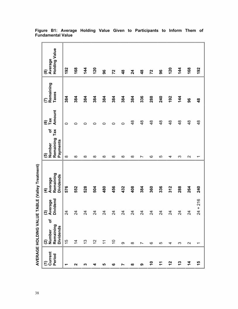
38

Figure B1: Average Holding Value Given to Participants to Inform Them of Fundamental Value

(8)

Ave

rage

H

oldi

ng V

alue

192

168

144

120

96

72

48

24

48

72

96

120

144

168

192

(7)

Rem

aini

ng

Taxe

s

384

384

384

384

384

384

384

384

336

288

240

192

144

96

48

(6)

Tax

Am

ount

0 0 0 0 0 0 0 48

48

48

48

48

48

48

48

(5)

Num

ber

of

Rem

aini

ng T

ax

Paym

ents

8 8 8 8 8 8 8 8 7 6 5 4 3 2 1

(4)

Ave

rage

R

emai

ning

D

ivid

ends

576

552

528

504

480

456

432

408

384

360

336

312

288

264

240

(3)

Ave

rage

D

ivid

end

24

24

24

24

24

24

24

24

24

24

24

24

24

24

24 +

216

(2)

Num

ber

of

Rem

aini

ng

Div

iden

ds

15

14

13

12

11

10

9 8 7 6 5 4 3 2 1

AVE

RA

GE

HO

LDIN

G V

ALU

E TA

BLE

(Val

ley

Trea

tmen

t)

(1)

Cur

rent

Pe

riod

1 2 3 4 5 6 7 8 9 10

11

12

13

14

15

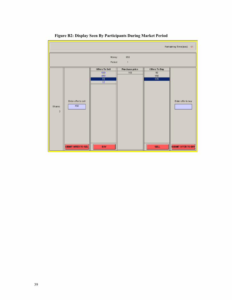
39

Figure B2: Display Seen By Participants During Market Period

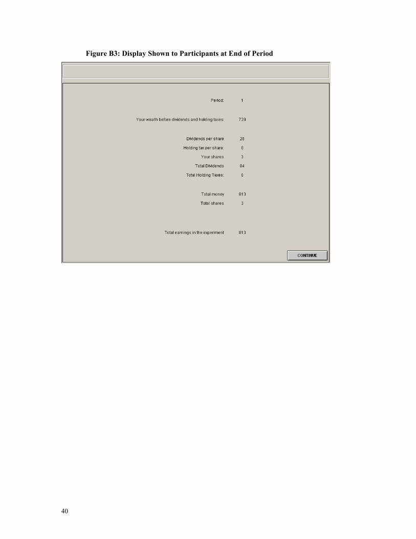
40

Figure B3: Display Shown to Participants at End of Period