PE281 Finite Element Method Course Notesweb.stanford.edu/class/energy281/FiniteElementMethod.pdf · PE281 Finite Element Method Course Notes summarized by Tara LaForce Stanford, CA

PE281 Finite Element Method Course Notes

summarized by Tara LaForce

Stanford, CA 23rd May 2006

1 Derivation of the Method

In order to derive the fundamental concepts of FEM we will start by lookingat an extremely simple ODE and approximate it using FEM.

1.1 The Model Problem

The model problem is:

−u′′ + u = x 0 < x < 1u (0) = 0 u (1) = 0

(1)

and this problem can be solved analytically: u (x) = x − sinhx/sinh1. Thepurpose of starting with this problem is to demonstrate the fundamentalconcepts and pitfalls in FEM in a situation where we know the correct answer,so that we will know where our approximation is good and where it is poor.In cases of practical interest we will look at ODEs and PDEs that are toocomplex to be solved analytically.

FEM doesn’t actually approximate the original equation, but rather the weak

form of the original equation. The purpose of the weak form is to satisfythe equation in the "average sense," so that we can approximate solutionsthat are discontinuous or otherwise poorly behaved. If a function u(x) is asolution to the original form of the ODE, then it also satisfies the weak formof the ODE. The weak form of Eq. 1 is

1

∫ 1

0

(−u′′ + u) vdx =

∫ 1

0

xvdx (2)

The function v(x) is called the weight function or test function. v(x) can beany function of x that is sufficiently well behaved for the integrals to exist.The set of all functions v that also have v(0) = 0, v(1) = 0 are denoted byH . (We will put many more constraints on v shortly.)

The new problem is to find u so that

∫ 1

0(−u′′ + u− x) vdx = 0 forallv ∈ H

u (0) = 0 u (1) = 0(3)

Once the problem is written in this way we can say that the solution u belongsto the class of trial functions which are denoted H . When the problem iswritten in this way the classes of test functions H and trial functions Hare not the same. For example, u must be twice differentiable and have theproperty that

∫ 1

0u′′vdx <∞, while v doesn’t even have to be continuous as

long as the integral in Eq. 3 exists and is finite. It is possible to approximateu in this way, but having to work with two different classes of functionsunnecessarily complicates the problem. In order to make sure that H and Hare the same we can observe that if v is sufficiently smooth then

∫ 1

0

−u′′vdx =

∫ 1

0

u′v′dx− u′v|10 (4)

This formulation must be valid since u must be twice differentiable and v wasarbitrary. This puts another constraint on v that it must be differentiableand that those derivatives must be well-enough behaved to ensure that theintegral

∫ 1

0u′v′dx exists. Moreover, since we decided from the outset that

v(0) = 0 and v(1) = 0, the second term in Eq. 4 is zero regardless of thebehavior of u′ at these points. The new problem is

∫ 1

0

(u′v′ + uv − xv) dx = 0. (5)

Notice that by performing the integration by parts we restricted the class oftest functions H by introducing v′ into the equation. We have simultaneouslyexpanded the class of trial functions H , since u is no longer required to have

2

a second derivative in Eq. 5. The weak formulation defined in Eq. 5 is calleda variational boundary-value problem.

In Eq. 5 u and v have exactly the same constraints on them:

1. u and v must be square integrable, that is:∫ 1

0uvdx ≈

∫ 1

0u2dx <∞

2. The first derivatives of u and v must be square integrable, that is:∫ 1

0u′v′dx ≈

∫ 1

0(u′)2dx <∞ (this actually guarantees the first property)

3. We had already assumed that v(0) = 0 and v(1) = 0 and we know fromthe original statement of the problem that u(0) = 0 and u(1) = 0.

Now we have that H = H = H10 . Any function w is a member of H1

0

if∫ 1

0(u′)2dx < ∞ and w(0) = w(1) = 0. H1

0 is the space of admissiblefunctions for the variational boundary-value problem (ie. all admissible testand trial functions are in H1

0 )

We will consider the variational form Eq. 5 to be the equation that we wouldlike to approximate, rather than the original statement in Eq. 1. Once wehave found a solution to Eq. 5 in this way we can ask the question whetherthis formulation is also a solution to Eq. 1: That is, whether this solution isa function satisfying Eq. 1 at every x in 0 < x < 1, or whether we have founda solution that satisfies only the weak form of the equation. In the case thatwe can only find a solution to the weak form, no "classical" solution exists.

1.2 Galerkin Approximations

We now have the problem re-stated so that we are looking for u ∈ H10 such

that

∫ 1

0

(u′v′ + uv) dx =

∫ 1

0

xvdx (6)

for all v ∈ H10 . In order to narrow down the number of functions we will

consider in our approximate solutions we will make two more assumptionsabout H1

0 . First, we will assume that H10 is a linear space of functions (that

is if v1, v2 ∈ H10 and a, b are constants then av1 + bv2 ∈ H1

0 .)

The second assumption is that H10 is infinite dimensional. For example if we

have the sine series ψn(x) =√

2sin(nπx) for n = 1, 2, 3, ... and v ∈ H10 then

3

v can be represented by v (x) =∑

∞

n=1 anψn (x). The scalar coefficients an

are given by an =∫ 1

0v (x)ψn (x) dx, just like usual. Hence infinititely many

coefficients an must be found to define v exactly. As in Fourier analysis,many of these coefficients will be zero. We will also truncate the series inorder to have managable length series, just like in discrete Fourier analysis.

Unlike in Fourier analysis, though the basis functions do not have to be sinesand cosines, much less smooth functions can be used. In fact our set of basisfunctions do not even have to be smooth and can contain discontinuities inthe derivatives, but they must be continuous. We will assume that the infiniteseries converges so that we can consider only the first N basis functions andget a good approximation vN of the original test (or trial) function:

v ∼= vN =∑N

i=1βiφi (x) (7)

where φi are as-yet unspecified basis functions. This subspace of functions isdenoted H

(N)0 and is a subspace of H1

0 . Galerkin’s method consists of finding

an approximate solution to Eq. 6 in a finite-dimensional subspace H(N)0 of

H(10 of admissible functions rather than in the whole space H1

0 . Now we arelooking for uN =

∑N

i=1 αiφi (x). The new approximate problem we have is

to find uN ∈ H(N)0 such that

∫ 1

0

(u′Nv′

N + uNvN) dx =

∫ 1

0

xvNdx (8)

for all vN ∈ H(N)0 . Since the φi are known (in principle) uN will be completely

determined once the coefficients αi have been found.

In order to find that αn we put∑N

i=1 αiφi (x) and∑N

i=1 βiφi (x) into Eq. 8.

∫ 1

0

ddx

[

∑N

i=1 βiφi (x)]

ddx

[

∑N

j=1 αjφi (x)]

+[

∑N

i=1 βiφi (x)] [

∑N

j=1 αjφi (x)]

−x

∑Ni=1 βiφi (x)

dx = 0 (9)

for all N independent sets of βi.

This can be expanded and factored to give

4

∑N

i=1βi

(

∑N

j=1

∫ 1

0

[

φ′

j (x)φ′

i (x) + φj (x)φi (x)]

dx

αj −∫ 1

0

xφi (x) dx

)

= 0

(10)

for all N independent sets of βi. The structure of Eq. 10 is easier to see if itis re-written as

∑N

i=1βi

(

∑N

j=1Kijαj − Fi

)

= 0 (11)

for all βi. Where

Kij =∫ 1

0

[

φ′

j (x)φ′

i (x) + φj (x)φi (x)]

dx F =

∫ 1

0

xφi (x) dx (12)

and where i, j = 1, ..., N . The N × N matrix of Kij is called the stiffnessmatrix and the vector F is the load vector. Since the βi are known Kij andF can be calculated directly. But the βi were arbitrary so we can choose eachelement βi for each equation. For the first equation choose β1 = 1 and βn = 0for n 6= 1. Now

∑Nj=1K1jαj = F1. Similarly for the second equation choose

β2 = 1 and βn = 0 for n 6= 2 so that∑N

j=1K2jαj = F2. In this way we havechosen N independent equations that can be used to find the N unknownsαi. Moreover the N coefficients αi can be found from αj =

∑Nj=1 (K−1)jiFi

where (K−1)ji are the elements of the inverse of K.

The stiffness matrix K is symmetric for this simple problem, which makesthe computation of the matrix faster since we don’t have to compute all ofthe elements, symmetric matricies are also much faster to invert.

1.3 Finite Elements Basis Functions

Now we have done a great deal of work, but it may not seem like we aremuch closer to finding a solution to the original ODE since we still knownothing about φi. The purpose of using such a general formulation is thatany set of linearly independent functions will work to solve the ODE. Nowwe are finally going to talk about what kind of functions we will want to useas basis functions. The finite element method is a general and systematictechnique for constructing basis functions for Galerkin approximations. In

5

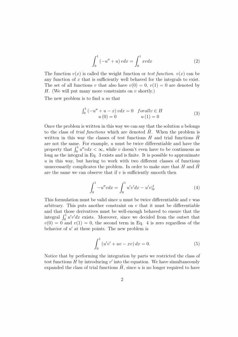
FEM the basis functions φi are defined piecewise over subregions. Over anysubdomain the φi will be chosen to be polynomials of low degree, thoughother possibilities do exist.

• finite elements are the subregions of the domain over which each basisfunction is defined. Hence each basis function has compact support overan element. Each element has length h. The lengths of the elementsdo NOT need to be the same (but generally we will assume that theyare.)

• nodes or nodal points are defined within each element. In Figure 1 thefive nodes are the endpoints of each element (numbered 0 to 4).

• the finite element mesh is the collection of elements and nodal pointsthat make up the domain and is shown in Figure 1. An element i isdenoted by Ωi.

Now we need to construct the actual basis functions using the three criteriadefined before: 1) The basis functions are simple functions defined piecewiseover the finite element mesh, 2) the basis functions must be in the class of testfunctions H1

0 , and 3) The basis functions are chosen so that the parametersαi are the values of uN(x) at the nodal points.

The simplest set of basis functions are the “hat functions” on elements i =1, 2, 3.

φi (x) =

x−xi−1

hi

for xi−1 ≤ x ≤ xixi+1−x

hi+1for xi ≤ x ≤ xi+1

0 for x < xi−1, x > xi+1

(13)

where hi = xi − xi−1 is the length of element i. The derivatives are

φ′

i (x) =

1hi

for xi−1 ≤ x ≤ xi−1

hi+1for xi ≤ x ≤ xi+1

0 for x < xi−1, x > xi+1

(14)

The equations for elements 0 and 4 have been left out since we decided thatu(0) = u(1) = 1, so no basis functions are required. In general the basisfunctions for the first and last elements are half of the functions since there

6

is no i−1 or i+1 node, respectively. The hat functions are shown in Figure 2.The mathematical term for hat functions is piece-wise linear basis functions

0 1 2 3 4

h1

h2

h3 h

4

Ω1 Ω2Ω3

Ω4

Figure 1: Four finite elements on the interval [0 1].

0 1 2 3 4−1

0

1

h1

h2

h3 h

4

Ω1 Ω2Ω3

Ω4

φ1 φ2φ3

0 1 2 3 4

−1

0

1

h1

h2

h3 h

4

Ω1 Ω2Ω3

Ω4

φ1∗ φ2

∗ φ3∗

Figure 2: Four hat functions (top) and their derivatives (bottom) on the interval [0 1].

Looking at the three criteria above, clearly the functions in Eq. 13 are simpleand defined element-wise. It is easy to show that they are in H1

0 , since theyhave square-integrable first derivatives. They also satisfy the third criteriasince φi(xj) = 1 if i = j and 0 otherwise. Hence each function contributes tothe value of uN at exactly one node and αi = uN(xi).

It is less clear that the hat functions will give a continuous representationof vN and uN . Let v be the sine function with period 2 shown in Figure

7

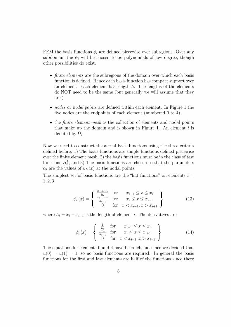
3. At the nodes (0, 1, 2, 3, 4) sine has the values (0,0.7071,1,0.7071,0).The representation vN on the finite element mesh is vN = 0.7071φ1 (x) +φ2 (x) + 0.7071φ3 (x). When the elements are summed up the sine waveis approximated by piecewise linear functions between each of the nodes,and is exactly represented at each node. When more nodes are used theapproximation improves and in the limit of N → ∞ the sine wave would beexactly represented. In FEM we will never proceed all the way to the limit,so the interval size h will always have finite size h. This is why the termfinite elements is used.

0 0.5 1 1.5 2 2.5 3 3.5 4

−1

0

1

h1

h2

h3 h

4

Ω1 Ω2Ω3

Ω4

0.7071φ1

φ2

0.7071φ3

sin(pi x)v

N

Figure 3: The finite element approximation of sin(πx) using five nodes on the interval[0 1].

1.4 The Stiffness Matrix K and the Load Vector F for

Hat Functions

Recall from Eq. 12 that each element of the stiffness matrix K is given by

Kij =∫ 1

0

(

φ′

i (x)φ′

j (x) + φi (x)φj (x))

dx

=∑4

e=1

∫

Ωe

(

φ′

i (x)φ′

j (x) + φi (x)φj (x))

dx

=∑4

e=1Keij

(15)

8

similarly

Fi =

∫ 1

0

xφi (x)dx =∑4

e=1

∫

Ωe

xφi (x)dx =∑4

e=1F e

i (16)

where we have used the property that φ(x) are defined piecewise on eachelement 1 through 4. In order to compute an approximation of the solutionto the model ODE it is necessary to compute nine elements for Kij fromi, j = 1, 2, 3 and three elements for F . But since each of the functions φ(x)are defined in the same way it is possible to compute Ke and F e for a genericelement and then to construct the matrix using the sums above. Consider ageneric interior element Ωe on the interval xA to xB. We will use a changeof variables and rewrite this in terms of ξ, a dummy variable for x. Wewill have ξ = (0, h). On this element exactly two of the hat functions arenonzero: ψA(ξ) = 1− ξ

hand ψB(ξ) = ξ

h. Convince yourself that this definition

is equivalent to the previous definition of the hat function, but with the originshifted to the start of one of the interior elements. The two hat functionshave derivatives ψ′

A(ξ) = − 1h

and ψ′

B(ξ) = 1h.

It is also important to notice that for the hat functions φi(x) 6= 0 on onlythe elements Ωi and Ωi+1. This results in a tridiagonal sparse matrix K forany number of elements in the mesh as will be shown below. Using Eq. 15you can see that there are three integrals that contribute to Kij :

kAA =∫ h

0

(

[ψeA′ (ξ)]2 + [ψe

A (ξ)]2)

dξ

=∫ h

0

(

[1/h]2 + [1 − ξ/h]2)

dξ = 1/h+ h/3

kAB =∫ h

0(ψe

A′ (ξ)ψe

B′ (ξ) + ψe

A (ξ)ψeB (ξ))dξ

=∫ h

0((−1/h) (1/h) + (1 − ξ/h) (ξ/h))dξ = −1/h+ h/6

kBB =∫ h

0

(

[ψeB′ (ξ)]2 + [ψe

B (ξ)]2)

dξ

=∫ h

0

(

[−1/h]2 + [ξ/h]2)

dξ = 1/h+ h/3

(17)

Similarly the components that contribute to the load vector are:

F eA =

∫ h

0(xA + ξ) (1 − ξ/h) dξ = h

6(2xA + xB)

F eB =

∫ h

0(xA + ξ) (ξ/h) dξ = h

6(xA + 2xB)

(18)

where the xA and xB terms come from evaluating the forcing function f(x) =x at the endpoints of the generic element.

9

Thus each generic interior element contributes to the stiffness matrix a 2× 2submatrix

ke =

[

1/h+ h/3 −1/h + h/6−1/h + h/6 1/h+ h/3

]

(19)

and two entries to the load vector

f e = h/6

[

2xA + xB

xA + 2xB

]

(20)

For the 4 element mesh we have derived the contributions to the overallstiffness matrix K from each node is given by:

K1 =

1/h+ h/3 0 00 0 00 0 0

K2 =

1/h+ h/3 −1/h+ h/6 0−1/h+ h/6 1/h + h/3 0

0 0 0

K3 =

0 0 00 1/h+ h/3 −1/h + h/60 −1/h + h/6 1/h+ h/3

K4 =

0 0 00 0 00 0 1/h+ h/3

(21)

where the contributions from elements 1 and 4 have only one entry becauseonly half of the hat function exists on these elements. Similarly the contri-butions to the load vector are

F 1 = h/6

2h00

F 2 = h/6

2h+ 2hh + 4h

0

(22)

F 3 = h/6

04h + 3h2h + 6h

F 4 = h/6

00

6h+ 4h

(23)

where h = 0.35 for the model problem. Now K = K1 + K2 + K3 + K4

and F = F 1 + F 2 + F 3 + F 4. The final system of equations has symmetricand diagonally dominant stiffness matrix K, which is very nice to work withmathematically. The values of uN at each node is given by α = K−1F anduN =

∑3i=1 αiφi (x).

10

Using this we get that the approximation to the model problem is u =0.0353φ1(x) + 0.0569φ2(x) + 0.0505φ3(x). This is not a very accurate an-swer, since only four elements were used. A more accurate approximationcan be obtained by using more elements, but at the cost of building andinverting a larger stiffness matrix K. The usual way of estimating the errorof an FEM approximation using linear basis functions (the hat functions wederived) using the L2 or mean-square norm is that ||e||0 < C2h

2. This is ana-priori error estimate and in general a worst-case scenario, the actual errormay be substantially smaller.

2 General One Dimensional Problems

At this point we will extend the derivation above to include general linearsecond-order elliptic ODEs of the form

ao (x)d2u (x)

dx2+ a1 (x)

du

dx+ a2 (x) u (x) = f (x) . (24)

Recall that this equation is elliptic if ao never changes sign or vanishes, ie|ao(x)| > γ > 0. We will also focus on two-point boundary-value problems

which are problems where half of the boundary conditions are specified ateach end point.

2.1 Flow Through Porous Media

One example in which elliptic boundary value problems arise in PE is asone-dimensional flow through porous media. Start by defining the flux σ ofthe fluid as σ(x) = −k(x)du

dx. σ can be a general flux function of any type,

but for porous media flow, u is hydraulic head or pressure, σ is the flowrate, k is the absolute permeability, f(x) is the fluid source/sink and mayrepresent wells or a boundary condition with flow across it, such as a constantflux boundary with an aquifer. In porous media flow we are also implicitlyassuming the additional equation for Darcy’s law holds, that is σ = −ku′.The permeability does not have to be constant in this formulation, but mayvary with x.

11

2.2 One-Dimensional Heat-Loss

One example in which elliptic boundary value problems arise in PE is heatloss from a wellbore. For the moment we can consider only 1D heat loss, butradial heat loss can be approximated using FEM as well. In heat loss u isthe temperature, σ is the heat flux given by Fourier’s law, f(x) is the heatsource (in this example, the wellbore), and k is the thermal conductivity ofthe porous medium.

2.3 Boundary Conditions

The most general boundary conditions that we will consider are

α0du(0)

dx+ β0u (0) = γ0

αldu(l)dx

+ βlu (l) = γl

(25)

Only the value of u is specified in a Dirichlet Boundary Condition. Onlythe value of du(0)

dxis specified in a Neumann Boundary Condition. The flux

−k(0)(−du(0)dx

) = σ0 or a linear combination of the flux and u are specified ina natural boundary condition.

Now we have a general ODE of the form

− d

dx

(

k (x)du (x)

dx

)

+ c (x)du

dx+ b (x) u (x) = f (x) (26)

where the second derivative of u has been replaced by the definition of theflux. This ODE doesn’t necessarily have a second derivative at every singlepoint in the domain since k(x) may not be continuous. u must have a secondderivative over every smooth sub-domain Ωi, but there may discontinuites atthe boundary between two subdomains. We didn’t worry about the existenceof the second derivative in the model problem in the last section because thereal physical problems we want to solve have the form of Eq. 26, with theboundary conditions defined in Eq. 25, not the form of Eq. 1.

As before, the ODE is multiplied by the test function v and integrated togive the variational form of the two-point boundary-value problem on anysmooth domain Ω

12

−ku′v|xi

xi−1+

∫

Ω

(ku′v′ + cu′v + buv) dx−∫

Ωi

fvdx = 0 (27)

If our domain is not smooth we can solve this problem over a series of sub-domains where the ODE is smooth and sum them. There are three types ofdiscontinuity that are possible at the edges of the Ω:

• k(x) is discontinuous, f(x) is continuous at x1. This gives a jumpcondition across the boundary of the element, but since k is finite onboth sides of the jump the flux is continuous and [σ (x)] = 0 at theboundary.

• f(x) is discontinuous, k(x) is continuous at x2. This gives a jumpcondition across the boundary of the element, but as long as f is finiteon both sides of the jump the flux is continuous and [σ (x)] = 0 at theboundary.

• f(x) is discontinuous at x3 and has a concentrated forcing term givenby the −f δ(x − xi) which is not finite. This gives a jump conditionacross the boundary of the element, and the flux is not continuous and[σ (x)] = f at the boundary.

As a consequence when we sum over all of the elements the variational bound-ary value problem becomes

k (0) u′ (0) v (0) − k (l)u′ (l) v (l) +∫ l

0(ku′v′ + cu′v + buv) dx

+ [σ (x1)] v (x1) + [σ (x2)] v (x2) + [σ (x3)] v (x3) =∫ l

0fvdx

(28)

At the points x1 and x2 the jump condition is zero so those terms drop out,but the jump at x3 is not zero, so we would have to deal with the f termin the FEM. For the rest of the derivation we will assume that we have nodiscontinuites of this type, but it is important to know that even very messydomains can easily be handled using FEM.

Rewriting Eq. 28 so that the homogeneous ODE is on the left and the forcingand boundary terms are on the right gives

∫ l

0(ku′v′ + cu′v + buv) dx = −v (0) k (0) [γ0 − β0u (0)]/α0

+v (l) k (l) [γl − βlu (l)]/αl +∫ l

0fvdx+ f v (x3)

(29)

13

2.4 Galerkin Approximation

Exactly as in the first section we are looking for a finite set of basis functionsφ1, φ2, ..., φN to approximate uN ∈ H(N). In this case we are no longerrequiring that our basis functions have the property v(0) = v(l) = 0 becausethe ODE is not necessarily zero at the endpoints, and we want to have thesame test and trial functions. The stiffness matrix for Eq. 29 is given by

Kij =

∫ l

0

(

kφ′

iφ′

j + cφ′

jφi + bφjφi

)

dx (30)

where j = i or j = i+ 1 are the only nonzero entries. The load vector is

Fi =

∫ l

0

fφi (x)dx+ −φi (0) k (0) γ0/α0 + φi (l) k (l) γl/αl (31)

where φi(0) = 0 for every element except the first and φi(l) = 0 for everyelement except the last. Once again we will be looking only at linear shapefunctions, but since we are now using vN that do not have v(0) = v(l) = 0we are going to re-define the shape functions slightly so that the origin of theshifted coordinate system is at the center of the element and ξ = −1 at the leftendpoint and ξ = 1 at the right endpoint. Now the two functions defined on ageneric element Ωe are given by ψ1 (ξ) = 0.5 (1 − ξ) and ψ2 (ξ) = 0.5 (1 + ξ).This is exactly the same functions employed in the first section, except thatnow on the first and last elements the basis functions are no longer zero.The real purpose of redefining the hat functions in this way is that thisformulation allows for the easy definition of higher-order approximations.

Each element makes a contribution to the stiffness matrix of the form

keij =

∫ se

2

se

1

(

kψei′ (ξ)ψe

j′ (ξ) + cψe

j′ (ξ)ψe

i (ξ) + cψei (ξ)ψe

j (ξ))

dξ (32)

for j = i± 1 and contributes to the load vector

f ei =

∫ se

2

se

1

(

fψei (ξ)

)

dξ. (33)

Typically the integrals are computed numerically. We are ignoring the bound-ary conditions and any discontinuities in the data at this point.

14

For linear basis functions each element has two nodes that contribute, so thefirst element has two equations of the form

k111u1 + k1

12u2 = f 11

k121u1 + k1

22u2 = f 21

(34)

The ith interior node has two equations of the form

ki11ui−1 + ki

12ui = f i1

ki21ui−1 + ki

22ui = f i2

(35)

This gives a tridiagonal matrix K and a load vector F such that

K =

k111 k1

12 0 0k1

21 k122 + k2

11 k212 0

0 k221 k2

22 + k311 kN−1

12

0 0 kN−121 kN−1

22

F =

f 11

f 12 + f 2

1

f 22 + f 3

1

fN−12

(36)

Provided that there are no discontinuities in the initial data. (See the bookfor how to handle discontinuities.) This formulation isn’t complete becausedoesn’t account for any boundary conditions.

2.5 Natural Boundary Conditions

For general natural boundary conditions of the form

α0du(0)

dx+ β0u (0) = γ0

αldu(l)dx

+ βlu (l) = γl

(37)

the matrix-vector equation including boundary conditions is

k111 − k(0)β0

αok1

12 0 0

k121 k1

22 + k211 k2

12 00 k2

21 k222 + k3

11 kN−112

0 0 kN−121 kN−1

22 + k(l)βl

αl

u1

u2

u3

uN−1

=

f 11 − k(0)γ0

αo

f 12 + f 2

1

f 22 + f 3

1

fN−12 + k(l)γl

αl

(38)

15

2.6 Neumann Boundary Conditions

For Neumann Boundary Conditions the equation is identical to Eq.38 withβo = βl = 0.

2.7 Dirichlet Boundary Conditions

For Dirichlet Boundary conditions the matrix problem reduces to a smallerproblem. Since u(0) and u(l) are both specified we don’t have to solve forthem. The first and last rows do not need to be included in the equation,but the second and N − 2 row of the load vector must be adjusted so thatthe new matrix-vector problem is

k122 + k2

11 k212 0 0

k221 k2

22 + k311 k3

12 00 k3

21 k322 + k4

11 kN−212

0 0 kN−221 kN−2

22 + kN−111

u2

u3

u4

uN−2

=

f 12 + f 2

1 − k121

γo

βo

f 22 + f 3

1

f 32 + f 4

1

fN−22 + fN−1

1 − kN−1

12γl

βl

(39)

Any combination of boundary conditions is also possible, and each boundarycan be set up as described above independently of the other.

3 Higher-Order Approximations

In general it is possible to use any polynomial function to approximate thefunction on each element. In practice it is rarely desirable to use much higherthan quadratic basis functions because higher-order functions have too muchoscillation. In order to define basis functions of order n each element musthave n + 1 nodes. The ith shape functions for an nth order approximationfor the basis functions is

ψi (ξ) =(ξ − ξ1) (ξ − ξ2) . . . (ξ − ξi−1) (ξ − ξi+1) . . . (ξ − ξn+1)

(ξi − ξ1) (ξi − ξ2) . . . (ξi − ξi−1) (ξi − ξi+1) . . . (ξi − ξn+1)(40)

Each of these functions is one at the node ξi and zero at ξj for i 6= j, whichimplies that they are all linearly independent on the element. There are n+1

16

linearly independent shape functions on each element. Using this definitionwith n = 1 gives the linear basis functions discussed in section 2.4. For n = 2we have to define three nodes per element, two are at the ends of the elementand one is in the center. Now the three shape functions are ψ1(ξ) = 1

2ξ(ξ−1),

ψ2(ξ) = 1 − ξ2, and ψ3(ξ) = 12ξ(ξ + 1).

For higher-order approximations the matrix K is defined in the same way asfor linear elements except that now we have

ueh (x) =

∑Ne

j=1ue

jψej (x) (41)

on each element. Where Ne is the number of nodes per element. This meansthat now instead of having to find uh at two points on every element weneed to find uh at n + 1 points, which makes our matrix-vector problemconsiderably larger. Frequently higher order methods are worth the costbecause a higher-order approximation has error of order hn+1, and is stillcomputationally cheaper than dividing the grid into enough elements to getthe same error from a linear approxiamtion.

Consider, for example if the interval [0, 1] is divided up into four elements. Alinear approximation would contain 8 basis functions and have an error on theorder of h2 = 0.252 = 0.0625. A quadratic approximation would contain 12basis functions and have an error on the order of h3 = 0.253 = 0.015625. Inorder to get an error this small using linear approximations we would haveto divide the domain into eight elements so that h2 = 0.1252 = 0.015625,and we would have to compute 16 basis functions. Though the matrix-vectorproblem is the same size for linear elements with h = 0.125 and quadraticelements with h = 0.25, the quadratic formulation requires only 3/4 as manycomputations in order to assemble the matrix.

4 Two-Dimensional Problems

At long last it is time to solve some PDEs using FEM! Fortunately allof the concepts from the first two sections apply (almost) directly to two-dimensional problems. We will consider problems of the form

−∇ · k (∇u (x, y)) + b (x, y) u (x, y) = f (x, y) (42)

17

Where the negative sign ensures that we are solving an elliptic equation.Once again we will define a flux term σ(x, y) = k (∇u (x, y)). Where kis the material modulus. In porous media flow k would be the absolutepermeability, and in heat loss k would be thermal conductivity. As before,these do not need to be constants, or even continuous. However, we willrestrict our derivation to cases where k is either continuous, or at least nicelyenough behaved to not cause discontinuities in the flux. This is exactly whatwe did in solving ODEs.

We will formulate the PDE as a variational boundary-value problem by mul-tiplying by a test function v and integrating over the domain (this is now anintegral in two-dimensions!)

∫

Ω

[−∇ · k (∇u (x, y)) + b (x, y)u (x, y) − f (x, y)] vdxdy = 0 (43)

In order to get everything in terms of first derivatives like we did in ODEswe use the product rule for differentiation to show that

∇ · (vk∇u) = k∇u · ∇v + v∇ · (k∇u)v∇ · (k∇u) = ∇ · (vk∇u) − k∇u · ∇v (44)

which can be inserted into Eq. 43 to give

∫

Ω

[k∇u · ∇v + buv − fv] dxdy −∫

Ω

[∇ · (vk∇u)] dxdy = 0 (45)

Using the divergence theorem we obtain that

−∫

Ω

[∇ · (vk∇u)] dxdy = −∫

∂Ω

k∇u · nvds (46)

where ∂Ω is the boundary of Ω integrated counterclockwise. Now we havethe final variational boundary-value problem

∫

Ω

[k∇u · ∇v + buv − fv] dxdy −∫

∂Ω

k∂u (s)

∂nvds = 0 (47)

with boundary conditions

18

−k (s)∂u (s)

∂n= p (s) [u (s))] (48)

where s ∈ ∂Ω, the boundary of Ω.

4.1 Approximation Functions

The idea here is to represent the approximate solution uh(x, y) and testfunctions vh(x, y) by polynomials defined piecewise over geometrically simplesubdomains of Ω. In one-dimension this consisted of dividing the line between[0, l] up into parts. In two-dimensions there are many posssible choices ofsimple shapes that we could choose to divide up the domain into. We willonly consider trianglar and rectangular elements.

4.1.1 Two-Dimensional Problems on Triangular Mesh

The simplest possible choice of shape function in two dimensions is a linevh(x, y) = a1 + a2x + a3y. Three constants need to be found, which meansevery element must have three nodes. A triangle with nodes at the cornerswould be the simplest and most logical way to satisfy this constraint. More-over, if adjacent triangular elements are forced to share two nodes then thiswill define a continuous function across the element boundary.

Similarly if we wanted to use a quadratic shape function vh(x, y) = a1+a2x+a3y+ a4x

2 + a5xy+ a6y2 we have six parameters and a triangular mesh with

nodes at each corner and at the midpoints of each side of the tringle wouldbe a good choice.

4.1.2 Two-Dimensional Problems on Rectangular Mesh

Suppose instead that we wanted to use bilinear shape functions vh(x, y) =a1 +a2x+a3y+a4xy. In this case we need to specify four nodes per elementin order to find the four constants a1 to a4. The logical choice here would beto use rectangular elements with nodes defined at each corner. If adjacentelements are forced to share two nodes then this will define a continuousfunction across the element boundary.

19

There are infinitely many possible combinations of shape functions and ele-ments. Sometimes it is desirable to use more complicated shapes in the meshinstead of triangular or rectangular. We will restrict our analysis to linearfunctions on triangular mesh, since that is the simplest choice.

4.1.3 Shape Functions

In two dimensions there are three basic requirements for the shape functions(and they are almost the same as in the ODE):

• The approximation to u must be continuous across element boundaries.

• The shape functions ψei must each be one at exactly one node and zero

at all others.

• The basis functions must be square-integrable and have square-integrablefirst partial derivatives.

The linear function vh(x, y) = a1 + a2x + a3y defines a plane in space. Asa consequence the approximation of u will be made up of triangular shapedsegments of planes that are continuous.

Suppose that the corners of a triangular elements are given by (x1, y1) (x2, y2)and (x3, y3). The shape function ψ1 that one at (x1, y1) and zero at nodes(x2, y2) and (x3, y3) is found from the plane equation evaluated at each nodeand is

ψe1 (ξ) =

1

2Ae

[(x2y3 − x3y2) + (y2 − y3)x+ (x3 − x2) y] (49)

where Ae = x2y3 +x1y2 +x3y1−x2y1−x3y2−x1y3 is the area of the element.

Similarly, the shape functions that are one at the node (x2, y2) and (x3, y3)are ψ2 and ψ3 respectively.

ψe2 (ξ) = 1

2Ae[(x3y1 − x1y3) + (y3 − y1) x+ (x1 − x3) y]

ψe3 (ξ) = 1

2Ae[(x1y2 − x2y1) + (y1 − y2) x+ (x2 − x1) y]

(50)

20

4.2 Finite Element Approximations

In general we are trying to find uh (x, y) =∑N

j=1 ujφj (x, y) such that uj = uj

at the nodes on ∂Ωh and

∫

Ωh

[

k(

∂uh

∂x∂vh

∂x+ ∂uh

∂y∂vh

∂y

)

+ buhvh

]

dxdy +∫

∂Ωpuhvhds

=∫

Ωh

fvhdxdy +∫

∂Ωh

γvhds(51)

where γ = pu. The general boundary condition has been put into the integralequation.

As before, the stiffness matrix K is given by

Kij =

∫

Ωh

[

k

(

∂uh

∂x

∂vh

∂x+∂uh

∂y

∂vh

∂y

)

+ buhvh

]

dxdy +

∫

∂Ω

puhvhds (52)

and the load vector F is

Fi =

∫

Ωh

fvhdxdy +

∫

∂Ωh

γvhds (53)

Ignoring the boundary conditions for the moment, we can look at the struc-ture of the linear basis functions and see that each function vi will contributeto exactly three of the columns of K (ie it effects three of the uj) in row isince there are three nodes per element. Hence the element matrix ke are3 × 3 matricies and the element load vector f e is a 3 × 1 column vector.

Consider a generic element e. The contribution to the stiffness matrix fromthe first basis function v = ψ1 is given by

∫

Ωh

k

[

(ψx1α1 + ψx2α2 + ψx2α3)ψx1

+ (ψy1α1 + ψy2α2 + ψy2α3)ψy1

]

+b (ψ1α1 + ψ2α2 + ψ2α3)ψ1

dxdy = ke11α1 + ke

12α2 + ke13α3

ke11 =

∫

Ωh

[

k[

ψ2x1 + ψ2

y1

]

+ bψ21

]

dxdy

ke12 =

∫

Ωh

[k [ψx2ψx1 + ψy2ψy1] + bψ1ψ2] dxdy

ke13 =

∫

Ωh

[k [ψx3ψx1 + ψy3ψy1] + bψ1ψ3] dxdy

(54)

21

where ψyi is the derivative of ψi with respect to y etc. and ue (x, y) =∑3

j=1 αjψj . Similarly, the contribution to the stiffness matrix from the firstbasis function v = ψ2 is given by

ke21 = ke

12

ke22 =

∫

Ωh

[

k[

ψ2x2 + ψ2

y2

]

+ bψ22

]

dxdy

ke23 =

∫

Ωh

[k [ψx3ψx2 + ψy3ψy2] + bψ2ψ3] dxdy(55)

and the contribution from ψ3 is

ke31 = ke

13

ke32 = ke

23

ke33 =

∫

Ωh

[

k[

ψ2x3 + ψ2

y3

]

+ bψ23

]

dxdy(56)

the contribution to the load vector from each basis function on the elemente are

f e1 =

∫

Ωh

[fψ1] dxdyfe2 =

∫

Ωh

[fψ2] dxdyfe3 =

∫

Ωh

[fψ3] dxdy (57)

The contribution of the first element to the total stiffness matrix and loadvector are given by

K1 =

k111 k1

12 k113 0 0 0 0

k121 k1

22 k123 0 0 0 0

k131 k1

32 k133 0 0 0 0

0 0 0 0 0 0 00 0 0 0 0 0 00 0 0 0 0 0 00 0 0 0 0 0 0

F 1 =

f 11

f 12

f 13

0000

(58)

In the case of two-dimensional problems we can’t just add each elementmatrix to the diagonal like we did in one dimensional problems because ofthe locations of the nodes. Because the mesh is triangular elements andnodes don’t necessarily have a nice correspondence. For example element 6may have as its nodes 3, 5, and 6 as in the picture. In that case, the shapefunctions on Ω1 will only effect the value of u at nodes 3, 5, and 6. Thismeans that the contribution of the sixth element to the stiffness matrix andload vector are given by

22

K6 =

0 0 0 0 0 0 00 0 0 0 0 0 00 0 k6

11 0 k612 k6

13 00 0 0 0 0 0 00 0 k6

21 0 k622 k6

23 00 0 k6

31 0 k632 k6

33 00 0 0 0 0 0 0

F 6 =

00f 6

1

0f 6

2

f 63

0

(59)

For two-dimensional problems the stiffness matrix is no longer tridiagional.If the nodes and elements are carefully ordered it can usually be written sothat it is a sparse matrix with large blocks of zeros.

4.3 Boundary Conditions

The stiffness matrix and load vectors we have assembled do not include anyboundary conditions. Implementation of boundary conditions is conceptuallythe same as in one-dimensional problems: Neumann boundary conditionsare implemented by subtracting the flux term k(s)∂u(s)

∂nfrom the load vector.

Natural boundary conditions are implemented by subtracting the flux termk(s)∂u(s)

∂nfrom the load vector and subtracting the value p(s)u(s) from the

components of the matrix that are on the boundary. Dirichlet boundaryconditions are implemented by getting rid of the row and column for whichu is known and adding the known value to the neighboring load vectors. Inpractice this can get quite complicated because the boundary is specified onevery element that has one side on the edge of Ω. Moreover, the boundaryconditions are usually different for different parts of the domain.

4.4 Example

In order to clarify some of these concepts we will look at an example problem.The domain, nodes and elements are shown in Figure 4. The domain ofthis problem is a reservoir with a constant pressure (Dirichlet) boundarycondition along the x = 0 axis (Γ74) to model influx from an aquifer, whileno-flow (Neumann) boundaries exist everywhere else. The forcing term is asingle production well in element 6 with constant pressure. This can also bethought of as a boundary condition. The PDE we are going to solve is

23

−∇ · k (∇u (x, y)) = f (x, y) (60)

If we further assume that k = 1 is constant then this simplifies to the problem

−∇2u (x, y) = f (x, y)

f (x, y) =

u1 Ω6

0 elsewhere

u (x, y) = 0 on Γ41∂u(x,y)

∂n= 0 on Γ74,Γ12,Γ25,Γ56,Γ67

(61)

−0.5 0 0.5 1 1.5 2 2.5−0.5

0

0.5

1

1.5

2

2.5

(1)

(2)

(4)

(5)

(6)

(3)

1

2 5

6

74

3

Γ74

Γ67

Γ56

Γ25

Γ12

Γ41

Figure 4: A six element domain with seven nodes.

The stiffness matrix and load vector for this example are given by:

K =

K11 K12 K13 K14 0 0 0K21 K22 K23 0 K25 0 0K31 K32 K33 K34 K35 K36 K37

K41 0 K43 K44 0 0 K47

0 K52 K53 0 K55 K56 00 0 K63 0 K65 K66 K67

0 0 K73 K74 0 K76 K77

F =

00f 6

1

0f 6

2

f 63

0

(62)

24

when the boundary conditions are neglected. Each of the entries Kij is thesum of the contributions of hat function to u at node i. Since node 3 is amember of every element, the row K3,j and the column Ki,3 are both filled.

Imposing the boundary condition u1 = u4 = 0 on Γ41 shrinks this to a 5 × 5matrix problem

K22 K23 K25 0 0K32 K33 K35 K36 K37

K52 K53 K55 K56 00 K63 K63 K66 K67

0 K73 0 K76 K77

u2

u3

u5

u6

u7

=

F2

F3

F5

F6

F7

(63)

Since the remaining boundary conditions are no-flux they don’t make anycontribution to the load vector. If the boundaries were constant flux thenelements 1, 2, 4, 5, 6, and 7 of the load vector would have to have the knownflux subtracted off of them. This is analogous to the one-dimensional problemwith Neumann boundary conditions.

The above matrix problem can be solved by finding u = K−1F . In twodimensional problems this can be much harder to do than in 1D because thematrix has filled in and is no longer tri-diagional. In order to get a sufficientlyaccurate solution, the size of the matrix K for 2D problems is also generallymuch larger than for a 1D problem.

References

[1] Becker„ E. B. G. F. Carey, and J. T. Oden, Finite Elements an In-

troduction, Texas Institute for Computational Mechanics, UT Austin,1981.

25