MODIFIED ANT COLONY ALGORITHM FOR COMBINATIONAL LOGIC CIRCUITS DESIGN by BAMBANG ALI BASYAH SARIF A Thesis Presented to the DEANSHIP OF GRADUATE STUDIES In Partial Fulfillment of the Requirements for the Degree of MASTER OF SCIENCE IN COMPUTER ENGINEERING KING FAHD UNIVERSITY OF PETROLEUM & MINERALS Dhahran, Saudi Arabia November 2003

Welcome message from author
This document is posted to help you gain knowledge. Please leave a comment to let me know what you think about it! Share it to your friends and learn new things together.
Transcript
MODIFIED ANT COLONY ALGORITHM FORCOMBINATIONAL LOGIC CIRCUITS DESIGN
by
BAMBANG ALI BASYAH SARIF
A Thesis Presented to theDEANSHIP OF GRADUATE STUDIES
In Partial Fulfillment of the Requirementsfor the Degree of
MASTER OF SCIENCE
IN
COMPUTER ENGINEERING
KING FAHD UNIVERSITY OF PETROLEUM & MINERALS
Dhahran, Saudi Arabia
November 2003
KING FAHD UNIVERSITY OF PETROLEUM & MINERALS
DHAHRAN 31261, SAUDI ARABIA
DEANSHIP OF GRADUATE STUDIES
This thesis, written by
BAMBANG ALI BASYAH SARIF
under the direction of his Thesis Advisor and approved by his Thesis Committee,
has been presented to and accepted by the Dean of Graduate Studies, in partial
fulfillment of the requirements for the degree of
MASTER OF SCIENCE IN COMPUTER ENGINEERING
Thesis Committee
Prof. Mostafa Abd− El− Barr (Chairman)
Prof. Sadiq M. Sait (Co− Chairman)
Assoc. Prof. Alaaeldin A. M. Amin (Member)Prof. Sadiq M. SaitDepartment Chairman
Prof. Osama A. JannadiDean of Graduate Studies
Date

Dedicated as a humble tribute to
my beloved parents and to
the memory of my paternal grandfather.
iii

ACKNOWLEDGMENTS
First and foremost, all sincere praises and thanks are due to Allah, the most Benef-
icent and the most Merciful, who guided us to Islam and enabled me to complete
my thesis work. I make a humble effort to thank Allah for His endless blessings on
me, as His infinite blessings cannot be thanked for. I pray Allah to bestow peace on
his last prophet Muhammad (Sal-allah-’Alaihe-Wa-Sallam) and on all his righteous
followers till the day of judgement. After that comes the following.
This thesis is never possible without the help, encouragement, motivation, and
influence of a large number of people. Dr. Mostafa Abd-El-Barr, my advisor, taught
me many things, but most importantly, how to do research and how to write well.
He was an inexhaustible storehouse of knowledge, insight and help on just about
any subject. His influence pervades this thesis and I am deeply indebted to him for
being my advisor and for having a complete faith in me. Dr. Sadiq M. Sait, my
co-advisor for his constant encouragement, unlimited support and guidance during
the course of this thesis. Mr. Uthman Al-Saiari, my colleague, for providing me
with any kind of help. Also Dr. Alaaeldin A. Amin, my thesis committee member,
for his comments and critical review of the thesis.
I would like to pay a heartily tribute to all of my family members and especially
to my parents, who guided me during all my life endeavors. Their love and support
iv

motivated me to continue my education and achieve higher academic goals. Without
their moral support and sincere prayers, I would have been unable to accomplish
this task.
I acknowledge the academic and computing facilities provided by the Com-
puter Engineering Department of King Fahd University of Petroleum & Minerals
(KFUPM)
I would also to acknowledge the help of Dr. Carlos A. Coello for his valuable
discussion during the course of this thesis.
Finally, I appreciate the friendly support from all my colleagues at KFUPM. In
particular, I want to thank to Irman, Ya’u, Badawi, Sanaullah and Saqib, among
others.
v

Contents
ACKNOWLEDGMENTS iv
LIST OF TABLES xi
LIST OF FIGURES xiv
ABSTRACT (ENGLISH) xix
ABSTRACT (ARABIC) xx
1 INTRODUCTION 1
1.1 Conventional Logic Design . . . . . . . . . . . . . . . . . . . . . . . . 2
1.2 Evolutionary Logic Design . . . . . . . . . . . . . . . . . . . . . . . . 4
1.3 Motivation . . . . . . . . . . . . . . . . . . . . . . . . . . . . . . . . . 7
1.4 Structure of the Thesis . . . . . . . . . . . . . . . . . . . . . . . . . . 9
2 BACKGROUND MATERIAL 10
2.1 Logic Synthesis Algorithms . . . . . . . . . . . . . . . . . . . . . . . . 12
vi

2.2 Ant Colony Optimization Algorithm . . . . . . . . . . . . . . . . . . 15
2.3 The Multiobjective Optimization Problem . . . . . . . . . . . . . . . 27
2.4 Fuzzy Logic . . . . . . . . . . . . . . . . . . . . . . . . . . . . . . . . 30
2.4.1 Fuzzy Set Theory . . . . . . . . . . . . . . . . . . . . . . . . . 31
2.4.2 Multi-objective Optimization Using Fuzzy Logic . . . . . . . . 34
2.5 Concluding Remarks . . . . . . . . . . . . . . . . . . . . . . . . . . . 36
3 LITERATURE REVIEW 37
3.1 Introduction . . . . . . . . . . . . . . . . . . . . . . . . . . . . . . . . 37
3.2 Classification of Evolutionary Logic Design . . . . . . . . . . . . . . . 38
3.3 Existing ELD Techniques . . . . . . . . . . . . . . . . . . . . . . . . . 39
3.3.1 EAs Based ELD . . . . . . . . . . . . . . . . . . . . . . . . . . 40
3.3.2 ACO Based ELD . . . . . . . . . . . . . . . . . . . . . . . . . 46
3.3.3 Other Related Work . . . . . . . . . . . . . . . . . . . . . . . 50
3.4 Discussion . . . . . . . . . . . . . . . . . . . . . . . . . . . . . . . . . 51
3.5 Concluding Remarks . . . . . . . . . . . . . . . . . . . . . . . . . . . 54
4 PROBLEM AND COST FUNCTION FORMULATION 56
4.1 Problem Formulation . . . . . . . . . . . . . . . . . . . . . . . . . . . 56
4.2 Problem Statement . . . . . . . . . . . . . . . . . . . . . . . . . . . . 59
4.2.1 Assumptions . . . . . . . . . . . . . . . . . . . . . . . . . . . . 60
4.2.2 Input and Output . . . . . . . . . . . . . . . . . . . . . . . . . 61
vii

4.3 Cost Function Modeling . . . . . . . . . . . . . . . . . . . . . . . . . 62
4.3.1 Gate Count Cost Function . . . . . . . . . . . . . . . . . . . . 62
4.3.2 Area Cost Function . . . . . . . . . . . . . . . . . . . . . . . . 63
4.3.3 Delay Cost Function . . . . . . . . . . . . . . . . . . . . . . . 63
4.3.4 Power Consumption Cost Function . . . . . . . . . . . . . . . 65
4.4 Weighted Sum Fitness Function Calculation . . . . . . . . . . . . . . 67
4.4.1 Functional Fitness . . . . . . . . . . . . . . . . . . . . . . . . 67
4.4.2 Objective Fitness . . . . . . . . . . . . . . . . . . . . . . . . . 68
4.5 Fuzzy Fitness Function Calculation . . . . . . . . . . . . . . . . . . . 70
4.5.1 Functional Fitness . . . . . . . . . . . . . . . . . . . . . . . . 70
4.5.2 Objective Fitness . . . . . . . . . . . . . . . . . . . . . . . . . 70
4.6 Concluding Remarks . . . . . . . . . . . . . . . . . . . . . . . . . . . 79
5 ACO ALGORITHM FOR COMBINATIONAL LOGIC DESIGN 80
5.1 Introduction . . . . . . . . . . . . . . . . . . . . . . . . . . . . . . . . 80
5.2 Modified-ACO (MACO) for Logic Design . . . . . . . . . . . . . . . . 82
5.2.1 Circuit Encoding . . . . . . . . . . . . . . . . . . . . . . . . . 83
5.2.2 Modifications of the Ant Colony Algorithm . . . . . . . . . . . 84
5.2.3 Filling the Matrix . . . . . . . . . . . . . . . . . . . . . . . . . 88
5.2.4 Ant Activity . . . . . . . . . . . . . . . . . . . . . . . . . . . . 89
5.2.5 Removing the Unfit Cell . . . . . . . . . . . . . . . . . . . . . 92
viii

5.3 Improved-Modified ACO algorithm . . . . . . . . . . . . . . . . . . . 99
5.3.1 Dynamic Search Space . . . . . . . . . . . . . . . . . . . . . . 99
5.3.2 Perturbation . . . . . . . . . . . . . . . . . . . . . . . . . . . . 101
5.3.3 Residual Function . . . . . . . . . . . . . . . . . . . . . . . . . 106
5.4 Concluding Remarks . . . . . . . . . . . . . . . . . . . . . . . . . . . 113
6 EXPERIMENTS AND RESULTS 114
6.1 Experimental Setup . . . . . . . . . . . . . . . . . . . . . . . . . . . . 114
6.2 Performance of Different Fitness Calculation . . . . . . . . . . . . . . 116
6.2.1 Effect of Different Weighting Scheme . . . . . . . . . . . . . . 116
6.2.2 Effect of Different FF Calculations . . . . . . . . . . . . . . . 121
6.3 Dynamic Search Space . . . . . . . . . . . . . . . . . . . . . . . . . . 122
6.4 Residual Function . . . . . . . . . . . . . . . . . . . . . . . . . . . . . 125
6.5 Different Optimization Objectives . . . . . . . . . . . . . . . . . . . . 126
6.6 Concluding Remarks . . . . . . . . . . . . . . . . . . . . . . . . . . . 135
7 COMPARISON WITH EXISTING TECHNIQUES 136
7.1 Comparison with Existing ACO-based Technique . . . . . . . . . . . 136
7.1.1 Comparison of Design Rate . . . . . . . . . . . . . . . . . . . 137
7.1.2 Comparison of the Quality of Solutions . . . . . . . . . . . . . 138
7.1.3 Comparison of Execution Time . . . . . . . . . . . . . . . . . 141
7.2 Comparison with Existing Conventional Techniques . . . . . . . . . . 142
ix

7.3 Comparison with other Techniques . . . . . . . . . . . . . . . . . . . 149
7.3.1 Comparison with GAs . . . . . . . . . . . . . . . . . . . . . . 149
7.3.2 Comparison with SimE . . . . . . . . . . . . . . . . . . . . . . 152
7.4 Concluding Remarks . . . . . . . . . . . . . . . . . . . . . . . . . . . 154
8 CONCLUSIONS AND FUTURE DIRECTIONS 155
8.1 Conclusion . . . . . . . . . . . . . . . . . . . . . . . . . . . . . . . . . 156
8.2 Future Directions . . . . . . . . . . . . . . . . . . . . . . . . . . . . . 157
APPENDIX 159
A File Format and Circuit Used as Test Cases 159
A.1 Library File Format . . . . . . . . . . . . . . . . . . . . . . . . . . . . 159
A.2 Input File Format . . . . . . . . . . . . . . . . . . . . . . . . . . . . . 160
A.3 Randomly Generated Circuits . . . . . . . . . . . . . . . . . . . . . . 162
A.4 Benchmark Circuits . . . . . . . . . . . . . . . . . . . . . . . . . . . . 162
BIBLIOGRAPHY 164
VITA 177
x

List of Tables
2.1 Connectivity matrix of TSP example shown in Figure 2.3. . . . . . . 20
2.2 Heuristic value for each edge in Figure 2.3. . . . . . . . . . . . . . . . 21
2.3 Solutions built by the ant in the first iteration. . . . . . . . . . . . . . 23
2.4 Pheromone values for each edge after iteration 1. . . . . . . . . . . . 24
2.5 Solutions built by the ant in the second iteration. . . . . . . . . . . . 25
2.6 Pheromone values for each edge after iteration 2. . . . . . . . . . . . 25
3.1 Possible cell functions in [1, 2, 3, 4, 5]. . . . . . . . . . . . . . . . . . 42
5.1 Gate ID, gate name and output of the gate, considering input a and b. 83
5.2 AND decomposition table. . . . . . . . . . . . . . . . . . . . . . . . . 109
5.3 OR decomposition table. . . . . . . . . . . . . . . . . . . . . . . . . . 109
5.4 XOR decomposition table. . . . . . . . . . . . . . . . . . . . . . . . . 110
6.1 Summary of circuits used for the experiments. . . . . . . . . . . . . . 115
6.2 Experimental results for WF = 0.5. . . . . . . . . . . . . . . . . . . . 117
xi

6.3 Experimental results for WF = 0.75. . . . . . . . . . . . . . . . . . . 117
6.4 Experimental results for WF = 0.875. . . . . . . . . . . . . . . . . . 118
6.5 Experimental results for dynamic WF . . . . . . . . . . . . . . . . . . 120
6.6 Results obtained for different FF calculations. . . . . . . . . . . . . . 122
6.7 Experimental result for static and dynamic matrix in terms of design
rate and computation time. . . . . . . . . . . . . . . . . . . . . . . . 124
6.8 Area result obtained using static and dynamic matrix size. . . . . . . 124
6.9 Results obtained using IMACO algorithm. . . . . . . . . . . . . . . . 125
6.10 Results of different optimization objectives. . . . . . . . . . . . . . . . 130
6.11 Results of DOAPC experiments normalized with respect to results of
AODPC. . . . . . . . . . . . . . . . . . . . . . . . . . . . . . . . . . . 131
6.12 Results of POADC experiments normalized with respect to results of
AODPC. . . . . . . . . . . . . . . . . . . . . . . . . . . . . . . . . . . 133
7.1 Comparison with Coello [6] in terms of design rate. . . . . . . . . . . 137
7.2 Comparison with Coello [6] in terms of area, delay and power. . . . . 139
7.3 Comparison with Coello [6] in terms of execution time. . . . . . . . . 142
7.4 Comparison of IMACO and SIS in area optimization for single output
circuits. . . . . . . . . . . . . . . . . . . . . . . . . . . . . . . . . . . 143
7.5 Comparison of MACO and SIS in area optimization for multiple out-
put circuits. . . . . . . . . . . . . . . . . . . . . . . . . . . . . . . . . 145
xii

7.6 Comparison of IMACO and SIS in delay optimization for single out-
put circuits. . . . . . . . . . . . . . . . . . . . . . . . . . . . . . . . . 147
7.7 Comparison of MACO and SIS in delay optimization for multiple
output circuits. . . . . . . . . . . . . . . . . . . . . . . . . . . . . . . 147
7.8 Comparison with GAs [7] technique in terms of area, delay and power.150
7.9 Comparison with GA [7] technique in terms of execution time. . . . . 151
7.10 Comparison with SimE technique in terms of area, delay and power
for area optimization. . . . . . . . . . . . . . . . . . . . . . . . . . . . 152
7.11 Comparison with SimE technique in terms of area, delay and power
for delay optimization. . . . . . . . . . . . . . . . . . . . . . . . . . . 153
xiii

List of Figures
1.1 Design space: area/delay trade-off for 64-bit adder [8]. . . . . . . . . 3
1.2 Evolutionary design process [1]. . . . . . . . . . . . . . . . . . . . . . 5
1.3 Circuit design methodologies. . . . . . . . . . . . . . . . . . . . . . . 6
2.1 Double bridge experiment. (a) Ants start exploring the double bridge.
(b) Eventually most of the ants choose the shortest path [9]. . . . . . 16
2.2 Ant Colony Algorithm. . . . . . . . . . . . . . . . . . . . . . . . . . . 18
2.3 Example of a TSP problem. . . . . . . . . . . . . . . . . . . . . . . . 20
2.4 (a) Visualization of pheromone values and (b) Best solution built in
the first iteration. . . . . . . . . . . . . . . . . . . . . . . . . . . . . . 24
2.5 (a) Visualization of pheromone values and (b) Best solution built in
the second iteration. . . . . . . . . . . . . . . . . . . . . . . . . . . . 26
3.1 A mapping scheme used in [10]. . . . . . . . . . . . . . . . . . . . . . 40
3.2 Chromosome representation used by Miller et. al., [1, 2, 3, 4, 5]. . . . 41
3.3 Example of genotype-phenotype mapping used in [1, 2, 3, 4, 5]. . . . 43
xiv

3.4 Encoding of a cell used in [6, 7, 11]. . . . . . . . . . . . . . . . . . . . 44
3.5 Chromosome representation [12, 13]. . . . . . . . . . . . . . . . . . . 45
3.6 Macro blocks and its genotype representation in [12, 13]. . . . . . . . 45
3.7 Mutation operators proposed in [12, 13]. . . . . . . . . . . . . . . . . 46
3.8 The matrix’s state after the filling of the first column. . . . . . . . . . 48
3.9 The matrix’s state after the filling of all cells . . . . . . . . . . . . . . 48
3.10 The cells used in the solution by an ant. . . . . . . . . . . . . . . . . 49
3.11 Problems that may appear in matrix representation: (a) fitness of F1
< 1 (b) fitness of F2 = 1. . . . . . . . . . . . . . . . . . . . . . . . . 51
3.12 An evolved two-bit odd parity circuit. (a) Fitness of F1 = 0 (b)
Adding an inverter, fitness of F1 = 1 (c) Toggle the type of gate
(XNOR → XOR), fitness of F1 = 1 . . . . . . . . . . . . . . . . . . . 52
4.1 Membership function for area. . . . . . . . . . . . . . . . . . . . . . . 72
4.2 Membership function for delay. . . . . . . . . . . . . . . . . . . . . . 74
4.3 Membership function for power. . . . . . . . . . . . . . . . . . . . . . 76
4.4 Dynamic Wf calculation. . . . . . . . . . . . . . . . . . . . . . . . . . 78
5.1 Figure Illustrating some of the possible paths in function f . . . . . . 81
5.2 Representation of a cell in the matrix. . . . . . . . . . . . . . . . . . 83
5.3 Example of a circuit and its encoding. . . . . . . . . . . . . . . . . . 84
5.4 Nest cell and matrix M for ant to be traversed. . . . . . . . . . . . . 85
xv

5.5 Modified ACO algorithm for logic design. . . . . . . . . . . . . . . . 86
5.6 Procedure Filling the Matrix. . . . . . . . . . . . . . . . . . . . . . . 89
5.7 Result of Filling the Matrix Procedure in the First Iteration for Ex-
ample 1. . . . . . . . . . . . . . . . . . . . . . . . . . . . . . . . . . . 93
5.8 Removing of cells in the first iteration. . . . . . . . . . . . . . . . . . 97
5.9 Filling the matrix in the second iteration . . . . . . . . . . . . . . . . 98
5.10 The Use of Row and Column Adjustment. . . . . . . . . . . . . . . . 102
5.11 How the Neighboring Cells Affect the FFn of Cell(i, j). . . . . . . . . 103
5.12 Perturbation Procedure. . . . . . . . . . . . . . . . . . . . . . . . . . 104
5.13 Effect of perturbation on functional fitness value (a) FFn = 0.9375
(b) FFn = 1. . . . . . . . . . . . . . . . . . . . . . . . . . . . . . . . 105
5.14 Effect of perturbation on objective fitness (a) gate count = 10 (b)
gate count = 8. . . . . . . . . . . . . . . . . . . . . . . . . . . . . . . 105
5.15 Example of using the residual function. . . . . . . . . . . . . . . . . . 110
5.16 Decomposition procedure. . . . . . . . . . . . . . . . . . . . . . . . . 111
5.17 Improved-Modified ACO algorithm for logic design. . . . . . . . . . . 112
6.1 Behavior of functional fitness function for circuit1 in the first 2000
iterations using AODPC. . . . . . . . . . . . . . . . . . . . . . . . . . 128
6.2 Behavior of functional fitness function for circuit1 in the first 50 iter-
ations using AODPC. . . . . . . . . . . . . . . . . . . . . . . . . . . . 128
xvi

6.3 Behavior of objective fitness function for circuit1 in the first 50 iter-
ations using AODPC. . . . . . . . . . . . . . . . . . . . . . . . . . . . 129
6.4 Behavior of objective fitness function for circuit1 in iteration 50 to
iteration 200 using AODPC . . . . . . . . . . . . . . . . . . . . . . . 129
6.5 Normalized results of DOAPC for single output circuits. . . . . . . . 132
6.6 Normalized results of DOAPC for multiple output circuits. . . . . . . 132
6.7 Normalized results of POADC for single output circuits. . . . . . . . 134
6.8 Normalized results of POADC for multiple output circuits. . . . . . . 134
7.1 Results of MACO normalized with respect to Coello [6]. . . . . . . . 138
7.2 2-bit Multiplier obtained by Coello [6]. . . . . . . . . . . . . . . . . . 140
7.3 2-bit Multiplier obtained by MACO. . . . . . . . . . . . . . . . . . . 140
7.4 Results of IMACO with AODPC for single output functions, normal-
ized to SIS. . . . . . . . . . . . . . . . . . . . . . . . . . . . . . . . . 144
7.5 Results of MACO with AODPC for multiple outputs functions, nor-
malized to SIS. . . . . . . . . . . . . . . . . . . . . . . . . . . . . . . 146
7.6 Results of IMACO with DOAPC for single outputs functions, nor-
malized to SIS. . . . . . . . . . . . . . . . . . . . . . . . . . . . . . . 148
7.7 Results of MACO with DOAPC for multiple outputs functions, nor-
malized to SIS. . . . . . . . . . . . . . . . . . . . . . . . . . . . . . . 148
xvii

7.8 Comparison with GA: normalized area, delay and power are always
≤ 1. . . . . . . . . . . . . . . . . . . . . . . . . . . . . . . . . . . . . 151
xviii

THESIS ABSTRACT
Name: BAMBANG ALI BASYAH SARIF
Title: MODIFIED ANT COLONY ALGORITHM
FOR COMBINATIONAL LOGIC CIRCUITS DESIGN
Major Field: COMPUTER ENGINEERING
Date of Degree: November 2003
Evolutionary computation presents a new paradigm shift in hardware design and
synthesis. According to this paradigm, hardware design is pursued by deriving in-
spiration from biological organism. Instead of using human made models and tech-
niques, the new methodology employs search heuristics to develop efficient designs.
In this thesis, a multiobjective optimization for evolutionary logic design based on
Ant Colony optimization algorithm is proposed. The result obtained using the pro-
posed algorithms are compared to those obtained using existing evolutionary tech-
niques as well as conventional techniques. Area, delay, and power consumption are
used as performance measures based on which the proposed algorithms and the exist-
ing techniques are compared. It is shown that the designed circuits using the proposed
algorithms outperform those of the existing techniques.
MASTER OF SCIENCE DEGREE
King Fahd University of Petroleum & Minerals, Dhahran, Saudi Arabia.
November 2003
xix

xx
ملخص الرسالة
بامبنج علي باشا شريف : االسم
الرقمية ائروتصميم الد في المعدلةخوارزم مملكة النمل :عنوان الدراسة
اآلليهندسة الحاسب : التخصص
٢٠٠٣ نوفمبر : التخرج تاريخ
. الحية تقليد الكائنات إلى أدىهذا التحول الجذري . ةالرقمي ائروتصميم الد يقدم الحساب االرتقائي تحول جذري جديدا في
الرسالةفي هذه . عمليهتصميمي لتطوير االستدالل تستخدم البحث الجديدة الطريقة, صنع البشرتصميم منبدال من استخدام
النتائج التي تحصلنا . المتعددة األهداف باعتباراستخدمنا خوارزم مملكة النمل للحصول على تصاميم للدوائر الكهربائيه
استخدمت المستهلكة والطاقةالوقت , المساحة. التقليدية و االرتقائيةعليها من الخوارزم قارناها بمثيالتها من الطرق
. للمقارنةآمقاييس
درجة الماجستير في العلوم
الملك فهد للبترول و معادن الجامعة
المملكة العربية السعودية - ظهران
٢٠٠٣ برنوفم

Chapter 1
INTRODUCTION
Design of digital circuits can be stated as a process of assembling a collection of logic
components to perform a specified function optimized for a number of design objec-
tives and subject to some design constraints, with respect to a specific target tech-
nology. Unfortunately, current design systems tend to depend on domain-specific
knowledge, which is somewhat limited both by the training and experience of the
designer. On the other hand, iterative and evolutionary heuristics, with little do-
main knowledge, may allow us to search in a design space, apply some assumptions
and use domain-independent operators to generate candidate solutions. Therefore,
heuristics have a tendency to search for solutions in a much larger, and often richer
design space beyond the realms of the conventional design techniques.
Ant Colony Optimization (ACO) algorithm [14] is a new meta-heuristic that
combines distributed computation, auto-catalysis (positive feedback) and construc-
1

2
tive greediness in finding optimal solutions to combinatorial optimization problems.
Unlike Genetic Algorithms (GAs) [15], ACO involves cooperating agents. In ACO,
interaction between components of the designed system can be easily analyzed.
Some daemon actions or other heuristics can also be incorporated to further im-
prove the quality of solutions. In this context, the central claim of this thesis is:
ACO algorithm can provide a computational tool for the circuit design problem.
1.1 Conventional Logic Design
There are four stages in the production of integrated circuits. These are design,
fabrication, testing and packaging [8]. The design stage itself is divided into three
major tasks: modeling, synthesis and optimization, and validation. The modeling
task consists of casting an idea into a model, that specifies the functionality of the
circuit. Synthesis deals with refining an abstract model into a detailed one that has
all the specifications required. Optimization is performed to maximize some figures
of merits of the circuit that relate to its quality. Some of the important merits for
optimization are: area, delay, power, testability, and fault tolerance.
Circuit models can be classified in terms of levels of abstraction: architectural,
logical, and geometrical. Logic level model deals with all facets of combinational and
sequential circuits. Logic synthesis can be defined as the manipulation of functional
specifications to a model as an interconnection of primitives components. In other

3
words, logic synthesis determines the gate-level structure of circuits. The classical
logic synthesis algorithms include the optimization of two quality measures, namely:
area and performance [16, 17, 18, 19, 20, 21, 22]. The design objective can be either
minimizing the area or maximizing the performance. Optimization can be subject to
constraints, such as upper bound on area, as well as upper bounds on performance
and lower bound on delay.
The possible configurations of a circuit are many. These different feasible struc-
tural implementations of a circuit define its design space. Figure 1.1 shows an
example design space of a 64-bit adder circuit, considering delay and area of the
circuit [8].
475
500
525
550
10 20 30 40 50
Area
Delay
Figure 1.1: Design space: area/delay trade-off for 64-bit adder [8].
The design space consists of a finite set of design points. A point in the design
space is called a Pareto point if there is no other point with at least an inferior objec-
tive, all others being inferior or equal [15]. This Pareto point can be easily observed
in a small design space, i.e., small circuit with few design objectives. However, if the

4
size of the circuit as well as the design objectives and/or constraints are increased,
the number of design points could be huge. Thus, it is more difficult to find the
most optimal structure for the given circuit. Hence, current available techniques
divide the circuit design problem into some sub-problems with lower dimensionality.
However, this approach is somehow constrained both by the training and experience
of the designer and by the amount of domain specific knowledge available. Thus,
the most optimal representation is unlikely to be obtained from this approach.
1.2 Evolutionary Logic Design
In conventional logic design, circuit designers begin with a precise specification in
the form of truth tables or Boolean expressions. These expressions are manipulated
by applying logic synthesis algorithms, such as factorization and kernel extraction
to minimize circuit representations. Therefore, the outcome of logic synthesis algo-
rithms will be either in two-level, multi-level, or Reed Muller representations.
Iterative heuristic is a non-deterministic algorithm that has a hill climbing prop-
erties. It has a mechanism to bias the search so as to improve the quality of solution.
Iterative heuristics work on a larger space that may not represent the desired func-
tion. Through the process of assemble and test, candidate solutions are built and
evaluated. At the end, an optimal solution could evolve from this process. Fig-
ure 1.2 shows evolutionary algorithms work on space that may not represent the

5
desired function, but gradually pulls the specification of the circuit towards the
target truth table.
Canonicalbooleanspace
OR
NOT
AND
R-M space
Space of alllogically correctrepresentations
The space of allrepresentations
n or lessvariables
EvolutionaryAlgorithms
Assembleand test
AppyingR-M rules
Applyingcannonical
rules
The space of alltruth tables of nor less variables
Figure 1.2: Evolutionary design process [1].
Furthermore, iterative heuristics may allow designers to define the search space of
circuit design in a way that is natural to both the problem and the implementation.
It may therefore be possible to use iterative heuristics to obtain novel designs that
are difficult to obtain using conventional techniques. Figure 1.3 shows the difference
between the conventional and the evolutionary methods for circuit design.
The first work in evolutionary design of digital circuits, Designer Genetic Algo-
rithms (DGA), was proposed by Louis [10]. This work has led to the establishment
of a new field of research called Evolvable Hardware (EHW) that was suggested by
Hugo de Garris [23]. Later, Zebullum et al. [24, 25], used Evolutionary Electronics
as the name for this field.

6
(a) Conventional techniques
(b) Evolutionary techniques
Figure 1.3: Circuit design methodologies.
Motivated by de Garris’s idea, Higuchi et al. [26] obtained an evolved circuit to
solve the 6-multiplexer problem [27]. Later in 1995, Thompson managed to evolve
a tone discriminator circuit in XC6200 FPGA [28]. He showed that Evolutionary
Algorithms were able to produce a tone discriminator circuit without input clock,
which is difficult to obtain by any conventional techniques. This work has hinted to
the possibility of a new method of designing circuits.
Koza et al. employed Genetic Programming (GP) [29] and pioneered the evo-
lution of analog circuits using a SPICE simulator. They were able to automati-
cally generate circuits which are competitive with those obtained using conventional
methods. They have shown further that it is possible to produce designs for quite
complex analog circuits, namely: low-distortion op-amps, low-pass filters, and band-
pass filters using GP [30].A functional level evolution was proposed by Higuchi [31].
A complete review and taxonomy of the field is described in [32, 24, 33].

7
In a recent development [11, 34], much attention has been given to the evolu-
tionary design of arithmetic circuits as they provide the essential building blocks
needed for larger DSP applications. Such effort has resulted in the development of
arithmetic circuits that range from a simple sequential adder to the more complex
3-bit multiplier. The work of Fogarty [35] and Miller [1] built some arithmetic cir-
cuits that cannot be produced by human designer’s conventional methods. Coello et
al. [11, 36] proposed a similar approach to evolve a circuit, which they showed was
better than that of Miller’s. Several other algorithms such as Ant Colony Optimiza-
tion, Cartesian Genetic Programming and Particle Swarm Optimization have also
been used for evolutionary logic design [6, 34, 37]. A complete review and taxonomy
of the field could be found in [24, 25, 33].
1.3 Motivation
The advent of evolutionary computation has created a new paradigm shift in logic
design and synthesis. It has radically changed the design procedure, and provided
the potential for discovering novel designs and/or more efficient circuits that are
beyond the scope of conventional methods.
Several approaches using evolutionary design of digital circuits were found in
literature. The results shown in the literature were promising. However, the exces-
sive runtimes and scalability characterize the use of iterative heuristics for any hard

8
combinatorial optimization problems. This provides incentive for investigating the
effectiveness of using iterative heuristics in logic design. In addition to that, there
are some other aspects that motivated this work. These aspects are listed below.
1. Multiobjective Optimization
Most of the existing techniques used the gate count as their optimization
objective. With the increasing need for circuits that have better performance
and lower power consumption, the objective of only minimizing the gate count
is not anymore acceptable. In addition, the term ‘gate’ or basic module for the
evolutionary logic design depends on the definition of the gate library that is
used. Therefore, optimizing the circuits in terms of area (delay and/or power)
is more appropriate compared to optimizing it in terms of gate count.
2. Heuristics Used
Most of the existing techniques in evolutionary logic design used Genetic Al-
gorithms (GAs) or Genetic Programming (GP) [30]. However, there exists
some other heuristics that are proved to be more efficient than GAs in solving
combinatorial optimization problems. These heuristics include the Ant Colony
Optimization (ACO) algorithm [14].

9
1.4 Structure of the Thesis
The rest of this thesis is organized as follows. Chapter 2 provides some background
material. Some definitions in logic synthesis and a brief overview of conventional
logic design are provided. The Ant Colony Optimization (ACO) algorithm is also
described in this chapter.
Chapter 3 presents a literature survey on existing techniques in evolutionary
design of combinational circuits. Observations, drawbacks, and possibility of im-
provements over the existing techniques are detailed in this chapter.
In Chapter 4, the multi-objective evolutionary logic design problem is formulated.
The calculation of area, delay and power consumption and their contribution to the
fitness function are designed.
The proposed algorithm for multi-objective evolutionary logic design problem
is described in Chapter 5. Chapter 6 provides the experiments and results of the
proposed techniques. Comparison with existing techniques is provided in Chapter
7. Finally, Chapter 8 provides some conclusions and possible future directions of
this work.

Chapter 2
BACKGROUND MATERIAL
The dramatic increase in designer productivity over the past decade in the area
of VLSI (Very Large Scale Integration) circuits can be attributed to the develop-
ment of sophisticated Computer Aided Design (CAD) tools. The improvement in
CAD tools has been made possible by the advances in the field of logic synthesis.
Logic synthesis techniques speed up the design cycle and reduce the human effort.
Logic Synthesis algorithms work on circuit model. Circuit representation is there-
fore important to understand [8]. In this chapter, we introduce some definitions and
terminology.
• Definition 2.1. A Boolean network is a directed acyclic graph that represents
a Boolean function f .
• Definition 2.2. A cube is a product of literals (ab, be, acd, ....).
10

11
• Definition 2.3. An algebraic expression is a non-redundant set of cubes.
Non-redundant means that no cube contains another; e.g. ab+ c is a non-redundant
expression while ab + b is a redundant expression because {b} ⊆ {a, b}.
• Definition 2.4. A Boolean function can be represented in the sum-of-product
(SOP) form or disjunctive normal form.
• Definition 2.5. A SOP expression is called cube-free if there exists no literal
that appears in all cubes in the expression.
For example, ab + ac is a cube-free SOP expression while ab + bc is not.
• Definition 2.6. Algebraic division is an operation used to compute a quotient
expression Q and a remainder expression R resulting from a given expression
F and divisor expression D such that F = Q ·D + R.
• Definition 2.7. Boolean division is an operation used to compute Q, D and R
of F (similar to algebraic division), using Boolean algebra rules.
• Definition 2.8. The Primary divisors of an expression F , denoted as D(F ),
are the set of quotients that are derived by dividing F by all possible cubes.
• Definition 2.9. The kernels of an expression F , denoted as K(F ), is the set of
cube-free primary divisors of F .

12
• Definition 2.10. The co-kernel is a cube that is used to derive a kernel.
Consider, for example, the function F = ae+ af + bce+ bcf + bde+ bdf . F/bc =
(e + f) is a kernel, and F/b = ce + cf + de is not. The co-kernel bc is used to obtain
kernel e + f .
Each kernel has its own level. The level of a kernel is defined according to the
following rules:
1. If a kernel does not contain any other kernel, the level of the kernel is 0.
2. If a kernel contains kernel of level n − 1 but does not contain kernels whose
level is more than n− 1, its level is n.
Consider the function F = ae + af + bce + bcf + bde + bdf . Function F can
be factorized to obtain F = (a + b(c + d))(e + f). K0 = c + d is a kernel of level
0, since it does not contain any other kernel. (e + f) is also a kernel of level 0.
K1 = (a + b(c + d)), while the function F itself is a level 2 kernel.
2.1 Logic Synthesis Algorithms
Early effort on logic synthesis and optimization algorithms are dated back to the
1950’s [16, 17] and 1960’s [38]. Although these efforts have much historical impor-
tance, their applicability was limited. However, as soon as Large Scale Integration

13
technology became available, the importance of logic synthesis was emphasized.
Many algorithms, such as MINI [39] and LSS [40] were proposed.
The advent of PLA (Programmable Logic Array) technology boosted the two-
level logic optimization techniques. ESPRESSO [18] is a well-known two-level logic
minimization tool.
The need for area minimization forces logic synthesis to consider the multi-level
logic representation. The introduction of kernel and kernel extraction techniques
in [19, 20] enhances the quality of multi-level logic optimization techniques. The
MIS [19] and BOLD [22] are examples of such techniques.
At the beginning of 1990s the area of logic synthesis matured. The most well
known logic synthesis tool, SIS, was proposed by Brayton et al. [21]. However, there
are some other recently introduced techniques that produce better quality results as
compared to SIS. The Perturb and Simplify [41] and Redundancy Addition and Re-
moval [42] are two such techniques. These techniques are based on the transduction
(transformation and reduction) method proposed by Muroga et. al. [43].
In addition to the common two-level and multi-level logic representations, there
exist some other techniques to represent Boolean functions. These include the
Binary Decision Diagrams (BDD) [38, 44, 45] and multiplexer based representa-
tions [46]. BDD is a directed acyclic graph (DAG) representation of logic functions.
Multi-level logic provides the optimal representation of Boolean functions in
terms of area. However, there are some Boolean functions that are more efficient

14
to implement using XOR-based representation as compared to the multi-level logic.
The n-bit parity checker is one such functions. The most well-known XOR-based
representation is the Reed-Muller (or AND-XOR) form [47]. There are fixed (positive
or negative) and mixed polarity RM forms. Unfortunately, decomposing Boolean
functions using XOR gates is difficult, let alone finding the perfect polarity for
it [48].
Recently, with several new power-constrained applications ranging from mobile
phones to laptop computers, power dissipation has emerged as another important
objective of VLSI circuit design [49, 50, 51]. The optimization of power consumption
can be performed at various levels of circuit design, including the logic level. Thus,
minimization of power consumption has to be reflected in the logic optimization
process. The POSE (Power Optimized Synthesis Environment) [52] is an example
of one technique that considers power consumption of the synthesized circuits.
With the increasing demand for high quality, more efficient and less area circuits,
circuit design has become a multiobjective optimization problem. Therefore, there
should evolve new methodologies for designing logic circuits. These should include
all types of representations, such as multi-level, Reed-Muller and multiplexer-based
representations. It should also consider all design objectives and/or constraints, such
as delay, area and power consumption. Therefore, logic synthesis can be modelled
as a search task in the design space. Deterministic algorithms are not favored due
to the huge size of the design space. The type of algorithms that could be used to

15
explore such huge search space size is non-deterministic algorithm. In this context,
the Ant Colony Optimization is a recent heuristic that deserves consideration.
2.2 Ant Colony Optimization Algorithm
The Ant Colony Optimization (ACO) algorithm is a new meta-heuristic that
has a combination of distributed computation, autocatalysis (positive feedback) and
constructive greediness to find an optimal solution for combinatorial optimization
problems. This algorithm tries to mimic the ants behavior in the real world. Since
its introduction, the ACO algorithm has received much attention and has been
incorporated in many optimization problems, namely the network routing, traveling
salesman, quadratic assignment, and resource allocation problems [14].
The ACO algorithm has been inspired by the experiments run by Goss et al. [53]
using a colony of real ants. They observed that real ants were able to select the
shortest path between their nest and food resource, in the existence of alternate
paths between the two. The search is made possible by an indirect communication
known as stigmergy amongst the ants. While traveling their way, ants deposit a
chemical substance, called pheromone, on the ground. When they arrive at a deci-
sion point, they make a probabilistic choice, biased by the intensity of pheromone
they smell. This behavior has an autocatalytic effect because of the very fact that
choosing a path will increase the probability that the corresponding path will be

16
Figure 2.1: Double bridge experiment. (a) Ants start exploring the double bridge.(b) Eventually most of the ants choose the shortest path [9].
chosen again by future ants. When they return back, the probability of choosing
the same path is higher (due to the increase of pheromone). New pheromone will be
released on the chosen path, which makes it more attractive for future ants. Shortly,
all ants will select the shortest path.
Figure 2.1 shows the behavior of ants in a double bridge experiment [9]. In
this case, because of the same pheromone laying mechanism, the shortest branch
is most often selected. The first ants to arrive at the food source are those that
took the two shortest branches. When these ants start their return trip, more
pheromone is present on the short branch than the one on the long branch. This
will stimulate successive ants to choose the short branch. Although a single ant is

17
in principle capable of building a solution (i.e., of finding a path between nest and
food resource), it is only the colony of ants that presents the “shortest path finding”
behavior. In a sense, this behavior is an emergent property of the ant colony.
This behavior was formulated as Ant System (AS) by Dorigo et al. [14]. Based on
the AS algorithm, the Ant Colony Optimization (ACO) algorithm was proposed [54].
In ACO algorithm, the optimization problem is formulated as a graph G = (C, L),
where C is the set of components of the problem, and L is the set of possible con-
nections or transitions among the elements of C. The solution is expressed in terms
of feasible paths on the graph G, with respect to a set of given constraints. The
population of agents (ants) collectively solve the problem under consideration us-
ing the graph representation. Though each ant is capable of finding a (probably
poor) solution, good quality solutions can emerge as a result of collective interac-
tion amongst ants. Pheromone trails encode a long-term memory about the whole
ant search process. Its value depends on the problem representation and the opti-
mization objective.
A general outline of the ACO algorithm is presented in Figure 2.2 [54]. Infor-
mally, the behavior of ants in ACO algorithm can be summarized as follows. A
colony of ants concurrently and asynchronously move through adjacent states of
the problem by moving through neighbor nodes of G. They move by applying a
stochastic local decision policy which makes use of the information contained in the
local node and ant’s routing table. By moving, ants incrementally build solutions

18
to the optimization problem. When the solution is being built, every ant evaluates
the solution and puts the information about its goodness on the pheromone trails
of the connection used. This pheromone information will direct the search of future
ants, until a feasible solution is found.
Algorithm ACO meta heuristic();while (termination criterion not satisfied)
ant generation and activity();pheromone evaporation();daemon actions(); {optional}
end whileend Algorithm
Figure 2.2: Ant Colony Algorithm.
The ants in ACO algorithm have the following properties [14]:
1. Each ant searches for a minimum cost feasible partial solution.
2. An ant k has a memory Mk that it can use to store information on the path it
followed so far. The stored information can be used to build feasible solutions,
evaluate solutions and retrace the path backward.
3. An ant k can be assigned a start state sks and more than one termination
conditions ek.
4. Ants start from a start state and move to feasible neighbor states, building
the solution in an incremental way. The procedure stops when at least one
termination condition ek for ant k is satisfied.

19
5. An ant k located in node i can move to node j chosen in a feasible neighborhood
Nki through probabilistic decision rules. This can be formulated as follows:
an ant k in state sr =< sr−1, i > can move to any node j in its feasible
neighborhood Nki , defined as Nk
i = {j | (j ∈ Ni) ∧ (< sr, j >∈ S)} sr ∈ S,
with S is a set of all states.
6. A probabilistic rule is a function of the following.
(a) the values stored in a node local data structure Ai = [aij] called ant-
routing table obtained from pheromone trails and heuristic values,
(b) the ant’s own memory from previous iteration, and
(c) the problem constraints.
7. When moving from node i to neighbor node j, the ant can update the pheromone
trails τij on the edge (i, j).
8. Once it has built a solution, an ant can retrace the same path backward,
update the pheromone trails and die.
In order to get more insight about the algorithm, an example of using ACO
algorithm for Traveling Salesman Problem (TSP) is given in the following.
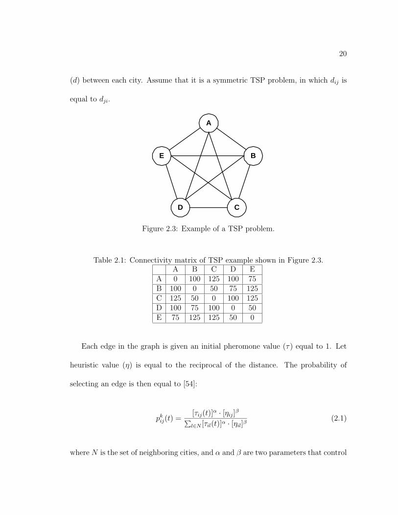
Consider, for example, a 5-city TSP problem shown in Figure 2.3. The objective
is to find the minimal tour required to visit all the 5 cities. The connectivity matrix
of the graph is given in Table 2.1. The values given in the table denotes the distance
20
(d) between each city. Assume that it is a symmetric TSP problem, in which dij is
equal to dji.
A
B
CD
E
Figure 2.3: Example of a TSP problem.
Table 2.1: Connectivity matrix of TSP example shown in Figure 2.3.A B C D E
A 0 100 125 100 75B 100 0 50 75 125C 125 50 0 100 125D 100 75 100 0 50E 75 125 125 50 0
Each edge in the graph is given an initial pheromone value (τ) equal to 1. Let
heuristic value (η) is equal to the reciprocal of the distance. The probability of
selecting an edge is then equal to [54]:
pkij(t) =
[τij(t)]α · [ηij]
β
∑l∈N [τil(t)]α · [ηil]β
(2.1)
where N is the set of neighboring cities, and α and β are two parameters that control

21
the relative weight of pheromone trail and heuristic value. In this example, for the
sake of simplicity, the value of α and β are set equal to 1.
Table 2.2 shows the heuristic value (η) for each edge.
Table 2.2: Heuristic value for each edge in Figure 2.3.A B C D E
A 0.000 0.010 0.008 0.010 0.013B 0.010 0.000 0.020 0.013 0.008C 0.008 0.020 0.000 0.010 0.008D 0.010 0.013 0.010 0.000 0.020E 0.013 0.008 0.008 0.020 0.000
Since there are 5 cities, assume that the size of the colony of ant is 5. Each ant
will start their tour from different city. For example, the first ant starts from city A,
the second ant starts from city B, and so on. The following explains how the ants
construct the solution.
Iteration 1
The first ant starts the tour from city A. There are four neighboring cities to be
considered by the ant. The probability of choosing any edge leading to a certain
city is calculated using Equation 2.1 and is given in the following table.
B C D E0.24 0.19 0.24 0.32
Using a stochastic process, i.e., Roulette Wheel, the ant choose the next city. Assume

22
that the ant takes city B as the next city to visit. The ant will update its memory
and put city B in its Tabu List
When the ant arrives at city B, there are 3 cities left to visit. The probability of
choosing these cities is given in the following table.
C D E0.48 0.32 0.19
Assume that city D is taken. The ant will then update its Tabu List by adding city
D.
There are two neighbors of city D: C and E. The following table shows the prob-
ability of choosing each of these cities.
C E0.33 0.66
Assume that the ant selects city E. The content of its Tabu List is then : A,B,D,E.
Since there is one remaining city to visit, the next process will certainly take C. The
path that was built by the ant is then: A → B → D → E → C. The length of this
path is L = AB + BD + DE + EC = 100 + 75 + 50 + 125 = 350.
The remaining ants will proceed according to the same procedure. The following
table summarize the solutions built by all ants.
The last column in Table 2.3 is the gain obtained by each ant. Since the longest

23
Table 2.3: Solutions built by the ant in the first iteration.Ant Path Length of the path (L) 4τ = 500/Lant1 A → B → D → E → C 350 1.43ant2 B → C → D → E → A 275 1.82ant3 C → B → D → E → A 250 2.00ant4 D → E → A → B → C 275 1.82ant5 E → A → B → C → D 325 1.54
distance between cities is 125. The solution built by the ant must not exceed 4 *
125 = 500. Thus, the gain of each ant can be formulated as 500/L, with L is the
length of the path of the solution.
When all ants finish their tour. They will track back and update the pheromone
along their path by putting additional pheromone (4τ). Note that, the amount of
4τ is proportional to the gain obtained by the ant. The new pheromone value is
given by the following.
τ = τ +4τ
Consider, for example, edge AB was used by ant1, ant4 and ant5. The new
pheromone value for edge AB is therefore equal to 1 + 1.43 + 1.82 + 1.54 = 5.79.
Then, pheromone will evaporate according to the following formula:
τ = (1− ρ) ∗ τ
Assume that ρ is equal to 0.2. Then the pheromone value on edge AB is equal to
0.8 * 5.79 = 4.63. The calculation of pheromone value is performed for all edges.

24
Table 2.4 shows the new pheromone values on each edge at the end of iteration 1.
Table 2.4: Pheromone values for each edge after iteration 1.initial pheromone value new pheromone value
A B C D E A B C D EA 0.00 1.00 1.00 1.00 1.00 0.00 4.63 0.80 0.80 6.54B 1.00 0.00 1.00 1.00 1.00 4.63 0.00 6.54 3.54 0.80C 1.00 1.00 0.00 1.00 1.00 0.80 6.54 0.00 0.80 0.80D 1.00 1.00 1.00 0.00 1.00 0.80 3.54 0.80 0.00 6.45E 1.00 1.00 0.80 1.00 0.00 6.54 0.80 0.80 6.45 0.00
A
B
CD
E
A
B
CD
E
(a) (b)
Figure 2.4: (a) Visualization of pheromone values and (b) Best solution built in thefirst iteration.
Figure 2.4 (a) shows the visualization of pheromone values on the edges. In this
figure, the darker the edge, the higher the pheromone. The best solution found by
the heuristic in the first iteration is shown in Figure 2.4 (b).
Iteration 2
The same process that were performed in the first iteration is repeated in the second
25
iteration. However, the initial pheromone values on all edges has changed. Thus, the
probability of selecting a certain edge will also change. The higher the pheromone
on the edge, the more attractive the edge for an ant to choose.
Assume that all ants have finished their tour construction. The following table
summarize the solutions built by all ants.
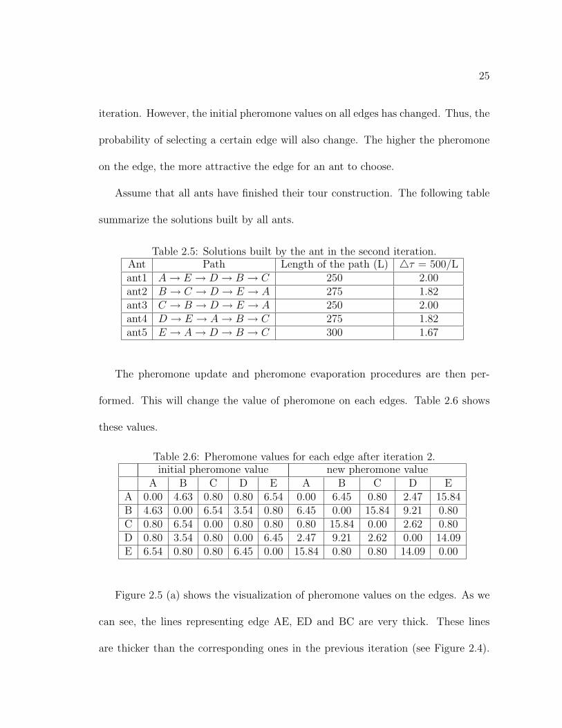
Table 2.5: Solutions built by the ant in the second iteration.Ant Path Length of the path (L) 4τ = 500/Lant1 A → E → D → B → C 250 2.00ant2 B → C → D → E → A 275 1.82ant3 C → B → D → E → A 250 2.00ant4 D → E → A → B → C 275 1.82ant5 E → A → D → B → C 300 1.67
The pheromone update and pheromone evaporation procedures are then per-
formed. This will change the value of pheromone on each edges. Table 2.6 shows
these values.
Table 2.6: Pheromone values for each edge after iteration 2.initial pheromone value new pheromone value
A B C D E A B C D EA 0.00 4.63 0.80 0.80 6.54 0.00 6.45 0.80 2.47 15.84B 4.63 0.00 6.54 3.54 0.80 6.45 0.00 15.84 9.21 0.80C 0.80 6.54 0.00 0.80 0.80 0.80 15.84 0.00 2.62 0.80D 0.80 3.54 0.80 0.00 6.45 2.47 9.21 2.62 0.00 14.09E 6.54 0.80 0.80 6.45 0.00 15.84 0.80 0.80 14.09 0.00
Figure 2.5 (a) shows the visualization of pheromone values on the edges. As we
can see, the lines representing edge AE, ED and BC are very thick. These lines
are thicker than the corresponding ones in the previous iteration (see Figure 2.4).

26
A
B
CD
E
A
B
CD
E
(a) (b)
Figure 2.5: (a) Visualization of pheromone values and (b) Best solution built in thesecond iteration.
The thickness of these lines correspond to their high pheromone values. This is
because more ants are using these edges (see Table 2.6). On the other hand, the
lines representing edge AC, BE and CE are very thin. Since no ant is using these
edges, there is no additional pheromone given. In addition, pheromone evaporation
reduces the intensity of pheromone values on these edges. This will make these edges
less attractive for future ants.
The algorithm will proceed until a criteria is met. From Figure 2.5(a), it can be
seen that the best solution for the given TSP problem will likely be equal to the one
illustrated in Figure 2.5(b).
It has been shown that ACO algorithm produced better quality results compared
to those obtained by other heuristics when it is applied to combinatorial optimization
problems such as TSP and QAP [55]. Unfortunately, only few published works found

27
in literature that uses ACO algorithm for evolutionary logic design (Coello et al.
[6]). Therefore, there is a need for investigating further the use ACO for evolutionary
design of digital circuits.
2.3 The Multiobjective Optimization Problem
Constraint satisfaction and multiobjective optimization are two aspects of the same
problem. Both involve the simultaneous optimization of a number of functions.
Based on the approach used in handling the constraint, there exists constrained
optimization and multiobjective optimization.
Constraints can be expressed in terms of inequalities of the type
f(x) ≤ g (2.2)
where f is a non-linear, real-valued function of the decision variable vector x, while
g is a constant value.
Without loss of generality, the constrained optimization problem is that of mini-
mizing a scalar function f1 of some decision variable vector x in a universe u, subject
to a number n−1 of conditions involving x, and eventually expressed as a functional
vector inequality of the type
(f2(x), ..., fn(x)) ≤ (g2, ..., gn) (2.3)

28
where the inequalities are applied component by component. It is assumed that
there is at least one point u which satisfies all constraints [56].
A general multiobjective optimization problem (MOP) includes a set of n parame-
ters (decision variables), a set of k objectives, and a set of m constraints. Objectives
and constraints are functions of the decision variables. The optimization goal is
defined in Equations 2.4, and 2.5.
maximize y = f(x) = (f1(x), f2(x), ..., fk(x)) (2.4)
subject to e(x) = (e1(x), e2(x), ..., em(x)) ≤ 0 (2.5)
Where,
x = (x1, x2, ..., xn) ∈ X (2.6)
y = (y1, y2, ..., yk) ∈ Y (2.7)
In this abstract model, x is called the decision vector, y is called the objective vector,
X is called the decision space, and Y is called the objective space. The constraints
e(x) ≤ 0 determine the set of feasible solutions. The feasible set Xf is defined as
the set of decision vectors x that satisfy the constraints e(x).
In order to select a suitable compromise solution from all alternatives, a decision
process is necessary in multiobjective optimization problems (MOP). The decision

29
process is performed based on the preference articulation. The preference articula-
tion implicitly defines the utility function to differentiate any candidate solutions.
Three approaches have been used, namely priorities, weighting coefficients and goal
values.
Priorities are real values, which determine the order in which objectives are to be
optimized according to their importance. In this technique, all objectives need to be
assigned different priorities. However, assigning priorities itself is another difficult
problem, mostly for conflicting objectives. Thus, the quality of results obtained
from this technique is rather limited.
In the weighting coefficient scheme, all objectives are aggregated into a single
function. An example of this approach is the weighted sum scheme given by:
min (k∑
i=1
wifi(x))
where wi ≥ 0 are the weighting coefficients representing the relative importance of
the ith objective function of the problem. It is usually assumed that:
k∑
i=1
wi = 1
This technique is known for its simplicity. However, since the result of solving
optimization model using weighted sum can vary significantly as the weighting co-

30
efficient change, the perfect tuning of weight values for each objectives become very
important. In addition, the different scale and behavior of each objective makes it
difficult to determine the perfect weights for each objective and aggregate them into
a single function.
The goal values can accommodate a whole variety of constrained and/or mul-
tiobjective problem formulations. The goal information is often naturally available
from the problem formulation, although not necessarily in an explicit way. The
interpretation of such information should be used to differentiate any alternate so-
lutions. The goal values can be easily incorporated with fuzzy logic [15] for solving
MOP problem. This will be explained in the following section.
2.4 Fuzzy Logic
Fuzzy Logic was introduced by Lofti A. Zadeh in [57, 58]. During the past decades,
fuzzy logic has found numerous applications in the field of engineering and control
[59]. In the field of VLSI design, several techniques based on fuzzy logic are reported
in the literature [60, 61, 62].
The expressive power of fuzzy logic derives from the fact that it contains not only
the classical two-valued and multi-valued logical systems but also probability theory
and probabilistic logic. Fuzzy logic deals with approximate rather than precise
modes of reasoning. This makes fuzzy logic capable of handling the uncertainty of

31
data. In addition to that, natural language, which is the basis of fuzzy logic, is more
convenient for expressing engineering problems.
In general, fuzzy logic can be viewed as a nonlinear mapping of an input data
vector into a scalar output. However, the flexibility of fuzzy logic may create lots of
different mapping for a single problem instance. Therefore, a good understanding
of the fuzzy set theory, fuzzy reasoning and fuzzy rules is needed.
2.4.1 Fuzzy Set Theory
Unlike in classical (crisp) theory where each element can either belong to the set
or not, an element in fuzzy logic may partially belong to a fuzzy set by a certain
degree.
A fuzzy set A of universe of discourse X is defined as A = {(x, µA(x)) | all x ∈
X}, where X is a space point and µA(x) is a membership function of x being an
element of A. A membership function µA(x) is a mapping of x in A that maps X
to the membership space M . The range of the membership function is a subset of
the non-negative real numbers whose boundaries are finite [63]. Elements with zero
degree of membership are normally not listed.
Fuzzy Reasoning
Unlike classical reasoning in which propositions are whether true of false, fuzzy logic
establishes approximate truth value of propositions based on linguistic variables and

32
inference rules [58]. A linguistic variable is a variable whose values are words or
sentences in natural or artificial language. It is concerned with the use of fuzzy
values that captures the meaning of words, human reasoning and decision-making.
An example of linguistic variable is circuit’s area. This variable can be expressed by
linguistic values like very small, small, average, large and very large circuit, rather
than 20 µm2, 30 µm2, 50 µm2, 75 µm2, and 100 µm2.
A linguistic variable carries the concept of fuzzy set qualifiers, called hedges.
Hedges are terms that modify the shape of fuzzy sets. They include adverbs such as
very, somewhat, quite, more or less, and slightly. They are used as modifiers, truth-
values, probabilities, quantifiers and/or possibilities of a certain linguistic variable.
Formally, a linguistic variable comprises of five elements [64]:
1. The variable name
2. The primary term set
3. The universe of discourse U
4. A set of syntactical rules that allows composition of the primary terms and
hedges to generate the term set
5. A set of semantic rules that assigns each element in the set a linguistic meaning.

33
Fuzzy Operators
There are two basic types of fuzzy operators. The operators for the intersection,
interpreted as the logical “and”, and the operators for the union, interpreted as the
logical “or” of fuzzy sets. The intersection operators are known as triangular norms
(t-norms), and union operator as triangular co-norms (t-co-norms or s-norms) [63].
Some examples of s-norm operators are given below, (were A and B are the fuzzy
sets of universe of discourse X).
1. Maximum. [µA⋃
B(x) = max{µA(x), µB(x)}].
2. Algebric sum. [µA⋃
B(x) = µA(x) + µB(x)− µA(x)µB(x)].
3. Bounded sum. [µA⋃
B(x) = min(1, µA(x) + µB(x))].
4. Drastic sum. [µA⋃
B(x) = µA(x) if µB(x) = 0, µB(x) if µA(x) = 0, 1 if
µA(x), µB(x) > 0].
An s-norm operator satisfies commutativity, monotonicity, associativity and µA⋃
0(x) =
µA(x) properties.
Following are some examples of t-norm operators.
1. Minimum. [µA⋂
B(x) = min{µA(x), µB(x)}].
2. Algebraic product. [µA⋂
B(x) = µA(x)µB(x)].
3. Bounded product. [µA⋂
B(x) = max(0, µA(x) + µB(x)− 1)].

34
4. Drastic product. [µA⋂
B(x) = µA(x) if µB(x) = 1, µB(x) if µA(x) = 1, 0 if
µA(x), µB(x) < 1].
Like s-norm, t-norms also satisfy commutativity, monotonicity, associativity and
µA⋂
1(x) = µA(x). Also, the fuzzy complementation operator is defined as follows.
µB(x) = 1− µB(x) (2.8)
2.4.2 Multi-objective Optimization Using Fuzzy Logic
Approximate reasoning can be made based on linguistic variables and their values.
Rules can be generated based on previous experience. The rules are expressed as
If ... Then statements. Connectives such as AND and OR can be used in approx-
imate reasoning to join two or more linguistic values. The If part (antecedent) is a
fuzzy predicate defined in terms of linguistic values and fuzzy operators (AND and
OR). The Then part is called the consequent.
In optimization problems, the linguistic value used in the consequent part iden-
tifies the fuzzy subset of good solutions. Therefore, the result of evaluation of the
antecedent part identifies the degree of membership in the fuzzy subset of good solu-
tions according to the fuzzy rule in question. If more than one rule is used to perform
decision-making, each rule can be evaluated to generate a numerical value. Then,
these numerical values from various evaluations of different rules can be combined

35
to generate a crisp value on a higher level of hierarchy.
Consider the circuit design problem with minimization of area, delay, and power
consumption. Three linguistic variables area, delay and power introduced. Then
good solutions can be characterized by the following fuzzy rule.
If the circuit has (small area) and (less delay) and (less power consump-
tion) then it is a good solution.
In the traditional fuzzy logic, the minmax operators are used to build the above
fuzzy rule. However, it was shown in [65] that these operators can lead to undesirable
behavior. This behavior has led to the development of other fuzzy operators such
as the Ordered Weighted Averaging (OWA) operator explained below.
Ordered Weighted Averaging (OWA) Operator
Generally, the formulation of multi criterion decision functions neither desires the
pure “AND-ing” of t-norm nor the pure “OR-ing” of s-norm. The reason for this is
the complete lack of compensation of t-norm for any partial fulfillment and complete
submission of s-norm to fulfillment of any criteria. Also the indifference to the
individual criterion of each of these two forms of operators led to the development
of Ordered Weighted Averaging (OWA) operators [66, 67]. This operator allows easy
adjustment of the degree of “AND-ing” and “OR-ing” embedded in the aggregation.
According to [66, 67], “OR-like” and “AND-like” OWA for two fuzzy sets A and B

36
are implemented as given in Equations 2.9 and 2.10 respectively.
µA∪B(x) = β ×max(µA, µB) + (1− β)× 1
2(µA + µB) (2.9)
µA∩B(x) = β ×min(µA, µB) + (1− β)× 1
2(µA + µB) (2.10)
where β is a constant parameter in the range [0,1]. It represents the degree to which
OWA operator resembles a pure “OR” or pure “AND” respectively.
2.5 Concluding Remarks
Some background material, definitions and concepts that should helpful in under-
standing this thesis work were provided in this chapter. Basic knowledge about
logic synthesis algorithm, Ant Colony Optimization (ACO) algorithm, MultiOb-
jective Optimization Problem (MOP) and Fuzzy Logic were also presented. Next,
literature review on existing techniques in ELD is given in Chapter 3.

Chapter 3
LITERATURE REVIEW
In this chapter, literature review of evolutionary logic design is presented. Discussion
and observations are also provided.
3.1 Introduction
In recent years, engineers have shown growing interest in Nature wishing to imitate
the observed processes. The reason for this lies in the fact that living beings exhibit
very desirable qualities, such as adaptation and fault tolerance which engineers have
been largely struggling to reproduce. This has led to the birth of such field as
evolutionary computation.
Recently, a new field of research in which hardware design is pursued as biological
organisms has begun to evolve. The new paradigm may radically change the design
37

38
procedure and new possibilities for discovering novel designs and/or more efficient
circuits may emerge. The new methodology considers a concept for automatic design
of electronic systems. Instead of using human made models and techniques, it
employs search heuristics to develop efficient designs.
Evolutionary design of digital circuits is a very challenging field. This is due
to two reasons: (a) the complexity of the search space and (b) the existence of
efficient CAD tools for digital design. Thus, it is difficult to develop new iterative
heuristics’-based CAD tools that provide competitive performance when compared
to the already existing ones. Nonetheless, the possibility to find new circuit designs
and the capacity to contemplate a larger set of specifications are some of the reasons
that complement its difficulty [25].
3.2 Classification of Evolutionary Logic Design
Evolvable Hardware (EHW) or Evolutionary Electronics is a field of research that
focuses on using Evolutionary Algorithms (EAs) in the hardware domain. The scope
of this field is vast, ranging from hardware design, fault tolerance, image processing
and pattern recognition to robot control [25, 33]. Nevertheless, EHW can be roughly
classified into two fields, namely design EHW and adaptive EHW. Based on the
application point of view, EHW is further divided into design of analog and digital
circuits. EHW for design of digital circuits is also called Evolutionary Logic Design

39
(ELD).
There are three possible representations of digital circuits in ELD, namely func-
tional, gate, and transistor level. These representations differ in the degree of com-
plexity of the basic building blocks used. On the functional level, a circuit is repre-
sented in terms of high level mapping of digital circuits. The basic building blocks
for this representation can be the minterms of a Boolean function or some RTL
blocks such as multiplexers. Gate level representation deals with basic logic gates,
while transistor level uses CMOS transistors and TTL as their building blocks.
Gate level representation is the most widely used representation in the literature.
This is due to the fact that the behavior of the basic building blocks, i.e., logic gates
is not as complicated as transistor level representation, as well as providing a simple
mapping between the circuit’s structure and the representation.
3.3 Existing ELD Techniques
Most of the techniques presented in the following section use Genetic Algorithms
(GAs) as the search engine for the ELD. Some adequate background on GAs can be
found in any book on iterative heuristic such as [15].

40
3.3.1 EAs Based ELD
Louis [10] introduced the idea of using Evolutionary Algorithms as tools to perform
structure design, in which digital circuits are viewed as structure of interconnected
logic gates. They modelled a given circuit as a matrix. Each cell represents a
primitive gate, such as AND, OR, NOT, and XOR gates with their corresponding
input. Connecting WIRES are simply gates that transfer one of their inputs to their
output. Every cell in a column i + 1 can only gets its input from cells in column i.
This structure is shown in Figure 3.1.
Input Output
Figure 3.1: A mapping scheme used in [10].
In this figure, gates which are close together in two-dimensional (phenotype)
space may be far apart in one-dimensional (genotype) space. This condition creates
problems for classical genetic operators such as single-point crossover. Therefore,
masked crossover is used to preserve highly fit schemas in the chromosome.
The masked crossover makes use of the relative fitness of the children, with
respect to their parents. When a child is produced, the masks used to produce it
may be modified depending on how well the child does relative to the parents. Initial
masks can be generated randomly and will be propagated along with the evolution

41
process. Mask propagation is controlled by a set of rules that depends on the relative
fitness of children to its parents. Thus, three types of children can be defined:
1. Good child: has fitness higher than that of both parents
2. Average child: has fitness between that of both parents
3. Bad child: has fitness lower than that of both parents.
A child’s mask is a copy of the dominant parent’s mask except for the changes
the rules allow. The underlying premise guiding the rules is that when a child is less
fit than its dominant parent, the recessive parent contributed bits reduce the fitness
of the child.
Using the above mentioned approaches, the authors managed to design some
digital circuits, ranging from 2-bit adders to 6-bit parity circuits [10].
Y1 Y2...... Yn
logic function
cells
......
input connectionsOutputs
11C 12C nmC
11C
21C
n1C
12C
22C
n2C
1mC
2mC
nmC
X1
X2
X3
Xn
Inputs OutputsInternal
connectionCells
Y3
Y2
Yn
Y1
Figure 3.2: Chromosome representation used by Miller et. al., [1, 2, 3, 4, 5].
Miller et al. [3] argued that one aspect of evolution in hardware is geometry.
They suggested that the chromosome representation should match the hardware’s

42
geometry configuration. In the case of FPGA, a matrix of n×m array of logic cells
is used as the phenotype representation. The genotype representation, the chromo-
some, is defined as a set of interconnections together with gate level functionality
for cells. This genotype-phenotype mapping is shown in Figure 3.2.
Since the authors were targeting FPGAs, the logic function at each gene of the
chromosome can be any of the possible functions realized by a FPGA cell. Table 3.1
lists all possible cell functions.
Table 3.1: Possible cell functions in [1, 2, 3, 4, 5].
Alphabet Function Alphabet Function
0 0 10 a⊕ b
1 1 11 a⊕ b
2 a 12 a + b
3 b 13 a + b
4 a 14 a + b
5 b 15 a + b
6 a · b 16 a · c + b · c7 a · b 17 a · c + b · c8 a · b 18 a · c + b · c9 a · b 19 a · c + b · c
Each gene is a sequence of integers representing the target interconnection of
gate’s inputs and the gate type. Consider, for example, the case shown in Figure 3.3.
The first quadruplet of the chromosome is 0-1-0-10, indicating that the first input
of the cell is connected to pin number 0, the second input to pin number 1, and
the third input to pin number 0 (the third input is not used) respectively. The gate
type is 10, two-input XOR. The interconnection between cells is restricted by the

43
levels-back parameter, which denotes the number of previous column(s) in the array
that a cell can be connected to. If the levels-back parameter is one, then each cell
must be connected to its immediate neighbor in the previous column. Cells within
any particular column cannot be connected together, and feedback connections are
not allowed.
Figure 3.3: Example of genotype-phenotype mapping used in [1, 2, 3, 4, 5].
The authors used Genetic Algorithm in [4] and Evolutionary Strategies in [1] to
produce some evolved circuits including those of a full adder and a 3-bit multiplier.
They have shown that the obtained circuits require fewer number of gates compared
to the ones produced using conventional methods.
Coello [6, 7, 11] used the same chromosome representation of circuits as
those used by Louis [10]. Each cell is a gate of the type AND, NOT, OR, XOR or
WIRE. Each cell is encoded in a triplet of inputs and gate type, as illustrated in
Figure 3.4.
A gate at position (i, j) of the matrix can only be connected to the one at

44
Input 1 Input 2 Gate type
Figure 3.4: Encoding of a cell used in [6, 7, 11].
(i, j − 1). This restriction reduces the cardinality of alphabet needed to represent
the chromosome, since the integer number to represent each cell is increasing in a
column wise only.
The evolution runs in two phases, the first phase is to find a fully functional
circuit, and the second one is to find an optimum circuit. The goal of the optimiza-
tion is to maximize the number of WIRES in the chromosome representation. This
translates into less number of gates required to implement a given circuit.
Coello proposed three different implementations of GAs, namely binary GA (BGA),
n-cardinality GA (NGA) and multiobjective GA (MGA). In MGA, multiobjective
optimization is not applied for optimizing different objectives such as delay, area
and power. It is used only to divide the search for correct truth table into several
objectives. Each optimization objective concentrates on a single bit in the truth
table. In addition, one optimization objective is added to unite all the former ones.
Thus, if the length of the truth table is n, then n + 1 objectives have to be found
by the MGA [36].
Hounsel et al. used a fixed length chromosome for circuit representation [12,
13]. Specific sections of the chromosome are reserved for describing the inputs
and outputs of the circuit. Circuit’s inputs are encoded in the first section of the

45
chromosome, while the outputs are defined at the end of the chromosome. Logic
elements are referenced by position within chromosome. Figure 3.5 displays the
relative location of each encoded section.
.... Positionalelement ....
Main circuit description Output sectionInput section
Input 1 Input n Output 1 Output k
Figure 3.5: Chromosome representation [12, 13].
Each logic element in a circuit is allocated at a specific position within the chro-
mosome. Each position can be a primitive gate or macro block such as multiplexer,
adder, etc. Each of these is represented by an ID from a circuit library. Intercon-
nectivity between cells is not restricted to its nearest positional neighbor. Rather,
cells are free to connect to other cells at higher positions within the chromosome.
Feedback connections are not permitted. Figure 3.6 demonstrates the encoding of a
macro block (full-adder) with its connectivity within the chromosome.
FULLADDER
In1
In 0Out 1
Out 0
In1
In 0Full AdderMacro ID
Positionof adder
Out 0Positionof NAND
In 0 In 1Positionof NOR
In 0
Position withinChromosome
Position of cell to whichfirst I/O pin is connected
ID from libraryof components
First I/O pinof full adder
I/P pin ofconnected cell
Figure 3.6: Macro blocks and its genotype representation in [12, 13].
Single point crossover is used to generate offsprings. Chromosome repair is used

46
to reconnect any broken interconnection during the operation. This guarantees
that an offspring chromosome represents a valid circuit. Mutation is applied to
maintain diversity within the population. There are four types of mutation used in
the evolution process. These are shown in Figure 3.7.
Aftermutation
After mutation
FULLADDER
FULLADDER
Cell Specific pin interchange
Ci
Ci
Si
Si
Connection interchangeCell replacement
new cell
old cell
Inter-chromosome cell mapping
Beforemutation
Figure 3.7: Mutation operators proposed in [12, 13].
Evaluation of chromosomes is done by a HDL simulator. The evolved circuit can
then be synthesized to provide a technology specific netlist, ready for transfer onto
the target FPGA. The evolved circuits have been compared with those designed
using conventional techniques. It is shown that some of the evolved circuits have
slightly better performance in terms of delay, compared to the circuits produced by
conventional methods [12, 13].
3.3.2 ACO Based ELD
ACO-based ELD was proposed by Coello et al. [6]. They used a matrix representa-
tion, whereby each cell of the matrix consists of a gate and the gate’s corresponding
input(s). Each column in the matrix is called a state and each cell in a certain

47
column is called a sub-state.
All ants have to construct a tour in each iteration. Ants start their movement
from the first column and proceed until they reach the last column. The goal of an
ant in constructing a tour is to fill up the matrix. However, ants can only fill the
first k (k is equal to the number of circuit’s output) number of cells in every column.
The other cells are filled randomly.
The selection of which attribute combination (gate type and its corresponding
input(s)) to be assigned in a newly visited cell is performed by a stochastic process.
For this purpose, all possible combinations of gates and its corresponding inputs are
considered. The probability of choosing a certain combination is determined by the
distance and pheromone value. The distance is the increment (or decrement) in the
number of correct matchings with the target truth table. The probability is then
calculated using the following formula.
pki,j(t) = fi,j(t)× hi,j (3.1)
where k refers to the ant that is considered, t refers to the current iteration, fi,j(t)
is the amount of pheromone between state i and state j, and hi,j(t) is the distance
between state i and state j. The selection is then performed by using roulette wheel.
Consider, for example, a two-bit adder circuit. Assume that the size of the matrix
used is 6 × 5. The number of inputs considered is four (without the carry input)
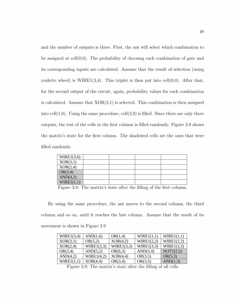
48
and the number of outputs is three. First, the ant will select which combination to
be assigned at cell(0,0). The probability of choosing each combination of gate and
its corresponding inputs are calculated. Assume that the result of selection (using
roulette wheel) is WIRE1(3,4). This triplet is then put into cell(0,0). After that,
for the second output of the circuit, again, probability values for each combination
is calculated. Assume that XOR(3,1) is selected. This combination is then assigned
into cell(1,0). Using the same procedure, cell(2,0) is filled. Since there are only three
outputs, the rest of the cells in the first column is filled randomly. Figure 3.8 shows
the matrix’s state for the first column. The shadowed cells are the ones that were
filled randomly.
WIRE1(3,6) XOR(3,1) XOR(2,4) OR(3,4) AND(4,2) WIRE1(1,1) Figure 3.8: The matrix’s state after the filling of the first column.
By using the same procedure, the ant moves to the second column, the third
column and so on, until it reaches the last column. Assume that the result of its
movement is shown in Figure 3.9
WIRE1(3,4) AND(1,6) OR(1,4) WIRE1(1,1) WIRE1(1,1) XOR(3,1) OR(5,2) XOR(4,2) WIRE1(2,2) WIRE1(2,2) XOR(2,4) WIRE1(3,3) WIRE1(3,3) WIRE1(3,3) WIRE1(3,3) OR(3,4) AND(5,2) OR(6,3) AND(3,4) NOT1(2,5) AND(4,2) WIRE1(4,2) XOR(4,4) OR(3,5) OR(5,3) WIRE1(1,1) XOR(4,4) OR(3,4) OR(3,5) AND(1,3) Figure 3.9: The matrix’s state after the filling of all cells

49
When the ants finish the tour, the solution obtained is evaluated. Note that
not all cells in the matrix are included in the final solution. Figure 3.10 shows an
example of tour built by an ant. In this figure, the shadowed cells are the ones that
are included in the final solution.
WIRE1(3,4) AND(1,6) OR(1,4) WIRE1(1,1) WIRE1(1,1) XOR(3,1) OR(5,2) XOR(4,2) WIRE1(2,2) WIRE1(2,2) XOR(2,4) WIRE1(3,3) WIRE1(3,3) WIRE1(3,3) WIRE1(3,3) OR(3,4) AND(5,2) OR(6,3) AND(3,4) NOT1(2,5) AND(4,2) WIRE1(4,2) XOR(4,4) OR(3,5) OR(5,3) WIRE1(1,1) XOR(4,4) OR(3,4) OR(3,5) AND(1,3) Figure 3.10: The cells used in the solution by an ant.
All ants will update the pheromone along its track. The pheromone update is
performed using the following formula.
fi,j(t + 1) = (1− α)× fi,j(t) +m∑
k=1
fki,j (3.2)
where 0 ≤ α ≤ 1, k is the index of the ant and fi,j of the solution built. The value
of fi,j is calculated based on the following conditions:
1. If the circuit is not feasible (i.e., not all outputs match their truth table).
fi,j(t) = fi,j(t) + payoff
2. If the circuit is feasible.
fi,j(t) = fi,j(t) + (2 × payoff)
3. If the circuit is the best feasible solution.

50
fi,j(t) = fi,j(t) + (3 × payoff)
The value of payoff is given by the number of matches produced between the output
generated by the circuit built by the agent and the target truth table. When all ants
finish their tour, the best solution is saved and the process starts from beginning
again. After the maximum number of iterations is reached, the best global solution
is returned.
3.3.3 Other Related Work
Multiplexer-based Genetic Programming for logic design was proposed by Coello
et al. [68]. A tree structure is used to represent a circuit. An algorithm, the Cartesian
Grid Programming (CGP), was proposed and used for logic design [69, 34]. A
complete automated system for ELD, “The Evolware” was proposed in [70].
Some researchers concentrated on the use of EAs for solving logic synthesis prob-
lems. Their work can be classified into three groups. The first group uses EAs to
optimize the representation of multi-level logic circuits [71, 72]. The second group
works on minimizing the RM representation using EAs [73, 74]. The last group
focuses on the optimization of BDD-based representation of logic circuits using
EAs [74].

51
a
b
c
F1
F2
a
b
c
F1F2
(a) (b)
Figure 3.11: Problems that may appear in matrix representation: (a) fitness of F1< 1 (b) fitness of F2 = 1.
3.4 Discussion
Several techniques in evolutionary logic design are described in the previous section.
Majority of those techniques were able to arrive at solutions that are difficult to
obtain using conventional methods. However, there are still many open problems
that were not addressed. A number of these problems are listed below.
1. Circuit representation
Most of the published work in evolutionary logic design used a two-dimensional
matrix of n × m to represent a circuit. The position of circuit’s outputs will
most likely be placed at cell(0,m− 1). However, it may happen that the best
solution can be found at cell(i, j), 0 < i < n, 0 < j < m. But some redundant
gates existing between this cell and the output cell may degrade the quality of
the solution. The problem becomes complicated even further when the number
of circuit’s output is more than one. Figure 3.11 illustrates the problem arises
from circuit representation.

52
a
b
c
F1
(a)
a
b
c
F1
(c)
a
b
c
F1
(b)
Figure 3.12: An evolved two-bit odd parity circuit. (a) Fitness of F1 = 0 (b) Addingan inverter, fitness of F1 = 1 (c) Toggle the type of gate (XNOR → XOR), fitnessof F1 = 1
2. Functional fitness calculation
The value of functional fitness depends on the number of correct matchings
between the output’s pattern of the obtained solution and the truth table
of the intended circuit. The higher the number of hits achieved, the higher
the value of the functional fitness. This argument is not always true in logic
design. A solution that has low functional fitness can be inverted to have a
high functional fitness (see Figure 3.12).
3. Don’t care values
A key factor in minimization of Boolean functions is the existence of don’t cares
value [20]. However, all techniques presented in ELD have paid no attention to
this factor. Their algorithms can only handle completely specified functions.
It is believed that the inclusion of don’t care values will be indeed beneficial
for the ELD.
4. Inverted inputs
Determining the correct phase (positive or negative) for each primary input

53
has been long addressed in conventional logic design techniques. In fact, for
some cases, the use of the complement of some of the primary inputs can lead
to more efficient circuit’s representation.
5. Objectives of the optimization
Most of the existing techniques used the gate count as their optimization
objective. With the increasing need for circuits that have better performance
and lower power consumption, the objective of only minimizing gate count is
not anymore sufficient. In addition, the term ‘gate’ or basic module for the
evolutionary logic design depends on the definition of the gate library that is
used. One may use NAND gates, or a set of AND, OR and XOR gates, or
MUXes, or a combination of them. Each of the aforementioned ‘gates’ has
different characteristics in terms of area, delay and input (output) capacitance
for different target technologies. Therefore, optimizing the circuits in terms of
area (delay and/or power) is more appropriate compared to optimizing it in
terms of gate count.
The ACO-based approach proposed in [6] shows some interesting features. The
problem associated with the circuit representation depicted in Figure 3.12 can be
handled. This is because whenever an ant visits a cell that has truth table equal
to the target truth table, the combination that will be selected for the next state
will most likely be WIREs. In addition, the number of combinations of attributes is

54
proportional to the size of the matrix and the number of gate types used. Therefore,
the process of assigning attributes to a new cell is a time consuming task.
In order to tackle the abovementioned problems, there are several possible im-
provements that can be investigated. These are enumerated below.
1. There is no need to fix the position of circuits output in the matrix. The ants
can stop anywhere in the matrix, whenever they found the fully functional
circuit.
2. The ant can have some intelligence to remember or forget some of the paths
that were built. Thus, in agreement with the first assumption, the ant can
return the best possible partial solution (sub-circuit) from the current matrix.
3. In order to support the second assumption, the content of the matrix will be
dynamically filled. At every iteration, the cells that were included in the best
possible partial solution obtained by the ant will be kept, while the other cells
will be removed. These empty cells will be filled again in the next iteration.
3.5 Concluding Remarks
In this chapter, several existing techniques in ELD have been presented. The review
has given insight on what has been done in this area. The discussion section in
this chapter has highlighted the shortcoming of those techniques and provided some

55
possible improvements. It has led us to propose a new technique in ELD. This is
the subject of the next chapter.

Chapter 4
PROBLEM AND COST
FUNCTION FORMULATION
In this chapter, the problem and cost function formulation are discussed. Problem
statement, assumptions, inputs and outputs of the designed approach are given.
4.1 Problem Formulation
A Boolean function can be represented in a number of forms. For example, the
following are possible representations of the same function.
1. f = xyz + xyz + xyz
2. f = (xy + xy)z + xyz
56
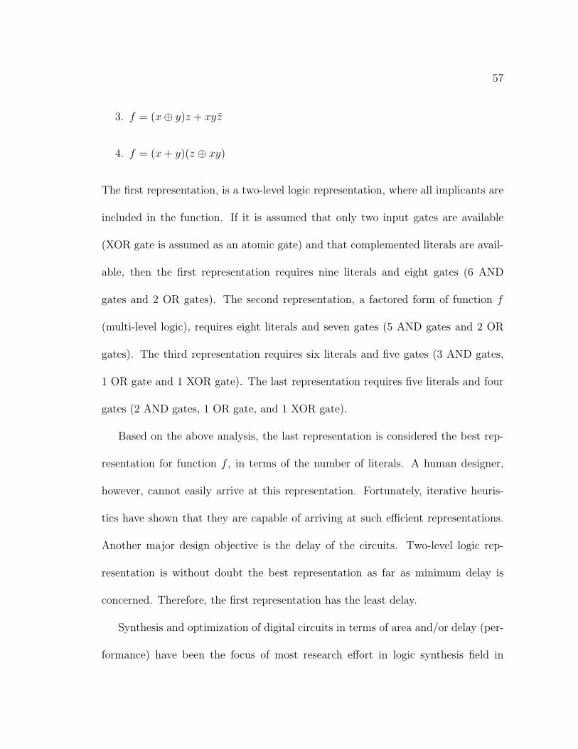
57
3. f = (x⊕ y)z + xyz
4. f = (x + y)(z ⊕ xy)
The first representation, is a two-level logic representation, where all implicants are
included in the function. If it is assumed that only two input gates are available
(XOR gate is assumed as an atomic gate) and that complemented literals are avail-
able, then the first representation requires nine literals and eight gates (6 AND
gates and 2 OR gates). The second representation, a factored form of function f
(multi-level logic), requires eight literals and seven gates (5 AND gates and 2 OR
gates). The third representation requires six literals and five gates (3 AND gates,
1 OR gate and 1 XOR gate). The last representation requires five literals and four
gates (2 AND gates, 1 OR gate, and 1 XOR gate).
Based on the above analysis, the last representation is considered the best rep-
resentation for function f , in terms of the number of literals. A human designer,
however, cannot easily arrive at this representation. Fortunately, iterative heuris-
tics have shown that they are capable of arriving at such efficient representations.
Another major design objective is the delay of the circuits. Two-level logic rep-
resentation is without doubt the best representation as far as minimum delay is
concerned. Therefore, the first representation has the least delay.
Synthesis and optimization of digital circuits in terms of area and/or delay (per-
formance) have been the focus of most research effort in logic synthesis field in

58
the last two decades. Results of several research efforts to optimize area and per-
formance are available in the literature and are summarized in several papers and
books [8, 19, 20, 21, 48]. Nevertheless, with several new power-constrained ap-
plications ranging from mobile phones to laptop computers, power dissipation has
emerged as a major objective of VLSI circuit design [49, 51]. Several published
works on logic synthesis targeting low power are reported in [52, 75, 76, 77, 78].
With the increasing demand of high quality, high performance and less area cir-
cuits, the problem of circuit design requires a multiobjective optimization approach.
However, it should be noted that optimal representation can be obtained by a care-
ful selection of gate types and an innovative ability to combine these in building a
circuit. However, this process is not an easy task. There are 22npossible n variables
single-output logic functions. This makes the complexity of circuit design problem
NP-hard.
Logic Design: A Search in the Design Space
As has been indicated in the preceding sections, the design space of digital circuits
could be huge. There are 2n (C2n
1 ) possible functions that satisfy 2n − 1 out of
2n correct truth table for an n-input single-output Boolean function. The number
of sub-functions that satisfy half of the truth table is C2n
2n/2. For example, there
are 12,870 possible sub-functions that satisfy half of the truth table of a four-input
Boolean function. The number of intermediate points in the design space that is not

59
representing the function is even bigger. In addition to that, there exists a number
of structures representing each of those points. These different structures represent
different design objectives and/or constraints. Exploring the whole search space is
impractical. Therefore, the search space sampled by the algorithm must have its
size limited.
Determining the size of the search space is a subtle issue. It should be large
enough to include a good variety of novel circuit topologies, but also small enough
for an iterative heuristic to be able to find good solution(s). Therefore, as stated in
[25], some procedures must be followed:
1. The search space sampled by the heuristics must have its size limited. Al-
though it is important to sample wide variety of topologies, some criteria
should be chosen to control the number of possible solutions.
2. It is usually necessary to adapt the search techniques to the particularities of
the design problem.
4.2 Problem Statement
Formally, the problem considered in this thesis can be stated as follows.
“Given the truth table of a function f of the required circuit and a
target technology to work within, design a combinational logic circuit

60
that performs the function f subject to a set of constraints using Ant
Colony Optimization (ACO) Algorithm”
The most efficient structural representation of a circuit will be chosen based
on the cost function used. It should be added that this work focuses on design of
combinational circuits. There are no memory elements and feedback paths allowed
in the circuit’s representation.
4.2.1 Assumptions
Here are some assumptions made before proceeding to the problem and cost function
formulation.
1. The set of logic gates used is available. Only two-input single-output logic
gates are considered. Wires are gates connecting one of its inputs to the
output.
2. The truth table or functional description of the intended Boolean function is
available.
3. The technology parameters are given.
4. The circuit is modelled as a matrix. Each cell of the matrix includes the
information about the gate type used and the index of cells in the previous
column which are connected to both of the gate’s inputs.

61
4.2.2 Input and Output
The proposed methodology in this thesis considers the following information as
inputs:
1. The truth table or functional description of the intended Boolean function
is available. The methodology can accept an input file consisting the truth
table of the circuit and parameters required by the heuristics. The file uses
the format described in Appendix A. The methodology can also accept a PLA
file of the circuit. In the case of random circuit experiments, all parameters
will be generated automatically, except for the number of variables, number
of outputs and number of experiments.
2. The file containing information of gates’ parameters is given. The format for
this file is given in Appendix A.
3. In order to have a comparison with SIS tools, the SIS environment should be
available to the system.
The outputs produced are as follows:
1. Structural representation of the logic gates in the matrix.
2. The quality measures of the final representation in terms of power consump-
tion, delay, number of gates used and area requirements.

62
The cost function that is used in this thesis includes area, delay and power
consumption of the circuits. The formulation of these cost function is explained
below.
4.3 Cost Function Modeling
This section discusses the modeling of cost functions in terms of gate count, area,
delay and power consumption.
4.3.1 Gate Count Cost Function
Each type of gate has different size, depending on the number of transistors used
to implement its function. The size of a NOT gate is different than the size of a
NAND gate. Thus, the number of gates cannot be used to estimate the area of a
given circuit. However, the increasing applicability of semi-custom VLSI circuits
complements that argument. In FPGAs, for example, a number of logic functions
can be implemented in one cell, regardless whether it is a NAND gate, an AND gate
or even a multiplexer. Therefore, for some target technology, the number of gates
can be used as one of the objective for optimization.
If G is the set of possible gate types and gi ∈ G, the cost for gate count can be
formalized as follows.
Costgate count =∑
gti (4.1)

63
Where
gti =
1 if gi ∈ G, gi 6= WIRE
0 otherwise
(4.2)
4.3.2 Area Cost Function
The size of a VLSI circuit consists of the area for logic gates (blocks) and the inter-
connection wires. With the advanced technology used for implementing VLSI cir-
cuits, the size of transistors become smaller and smaller. Thus, the area requirement
for interconnection wire becomes significant. However, the length of interconnection
wires in VLSI circuits is determined by routing algorithms. Therefore, in this thesis,
only area from logic gates is used to estimate the overall size of the circuit. The size
of these gates is obtained from a VLSI design library.
Formally, the cost for area of VLSI circuits can be stated as follows.
Costarea =∑
gi∈G, gi 6=WIRES
A(gi) (4.3)
Where A(gi) is the area of gate gi and gi ∈ G.
4.3.3 Delay Cost Function
The overall performance of a VLSI circuit depends upon how fast it can process
signals, i.e., its clock speed. The propagation delay of signals in VLSI circuits
consists of two elements: switching delay of gates and interconnect delay. Due to

64
improved technology, libraries with considerably low switching delay are available.
This fact and the increased gate density on the chip make the interconnect delay a
prominent factor in the overall circuit delay.
If a path π consists of nets {v1, v2, ..., vn}, then, the delay Tπ along π is expressed
by the following Equation.
Tπ =n−1∑
i=1
(CDi + IDi) (4.4)
Where CDi is the switching delay of the cell driving gate vi and IDi is the inter-
connect delay of net vi.
Using the RC delay model, IDi depends on the load factor, interconnect resis-
tance and load capacitance, as shown in Equation 4.5.
IDi = (LFi + Ri)× Ci (4.5)
Where LFi is the load factor of the driving block (which is independent of the
layout), Ri is the interconnect resistance of net vi, and Ci is the load capacitance of
cell i.
The load capacitance Ci of gate i comprises the interconnect capacitance at the
output node of gate i and the sum of the capacitances of the input nodes of the

65
gates driven by gate i.
Ci = Cri +
∑
j∈Mi
Cgj (4.6)
Where Cgj is the capacitance of the input node of a gate j driven by gate i and Cr
i
represents the interconnect capacitance at the output node of cell i.
The overall circuit delay is determined by the delay along the longest path (the
most critical path) in the layout. If the most critical path is denoted by πc then,
the cost function for the circuit delay can be given as follows.
Costdelay = Tπc = maxj{Tπj
} ∀j ∈ {1, 2, . . . , K} (4.7)
Where K represents the total number of critical paths determined by a timing
analysis program.
4.3.4 Power Consumption Cost Function
In a standard CMOS circuit, the total power consumption can be given by the
following Equation.
Pt =∑
i∈M
(1
2· Ci · V 2
DD · f · Si · β) +∑
i∈V
QSCi· VDD · f · Si + Ileak · VDD (4.8)
In Equation 4.8, Pt is the total power consumption, VDD is the supply voltage,

66
Si is the switching probability at the output node of cell i, i.e., the number of
transitions per clock cycle at the output of gate i and f is the clock frequency.
The first term in the above equation gives the dynamic power consumption during
charging or discharging of a node in the circuit. Here, M is the set of all nodes in
the circuit, Ci denotes the total capacitance of node i whereas β is a technology
dependent constant. The second term in Equation 4.8 gives the power consumption
due to the short circuit current. Here, V is the set of all wires connecting VDD
to ground during output transition, QSCirepresents the charge carried by the short
circuit current per transition. The third term represents the static power dissipation
due to leakage current Ileak.
In the VLSI circuits with well designed logic gates, the dynamic power consump-
tion contributes about 90% to the total power consumption [79]. Hence, most of
the reported work is focused on minimizing the dynamic power consumption. Also,
in the case of standard-cell placement, the cells are obtained from the technology
library and nothing can be done to reduce the power consumption due to the second
and the third term in Equation 4.8. Due to this fact, the emphasis in this work is
on optimizing the dynamic power consumption. Since the first term is dominant,
Equation 4.8 can be approximated as follows.
Pt '∑
i∈M
1
2· Ci · V 2
DD · f · Si · β (4.9)

67
Assuming the clock frequency and input voltage to be fixed, the total power con-
sumption of the circuit becomes a function of the total capacitance and the switching
probabilities as shown below.
Pt '∑
i∈M
Ci · Si (4.10)
Thus, the estimate of cost of the overall power consumption in VLSI circuits can
be approximated as follows.
Costpower =∑
i∈M
Si · Ci (4.11)
4.4 Weighted Sum Fitness Function Calculation
The fitness of a solution contains two parts, namely functional fitness and objective
fitness. The functional fitness deals with the functionality of the solution, i.e., how
good the solution is in satisfying the truth table of the intended Boolean function.
The objective fitness determines the quality of solution in terms of delay, area,
and/or power consumption.
4.4.1 Functional Fitness
Several functional fitness formulations are reported in the literature [25]. The com-
monly used one is the ratio of the number of correct hits to the length of the truth

68
table. If FF denotes the functional fitness, then the formulation below is applied.
FF =Number of hits
Length of the truth table(4.12)
The solution has to be ‘inverted’ if the value of FF is less than 0.5. Therefore, the
formulation of normalized FF (FFn) below is applied.
FFn = Max{FF, 1− FF} (4.13)
4.4.2 Objective Fitness
The objective fitness (OF (i)) is a measure of the quality of solution in terms of
optimization objectives such as area, delay, gate count, and power consumption.
It consider two aspects: constraints satisfaction and multiobjective optimization.
In order to indicate whether a solution is satisfying a certain constraint, objective
fitness is formulated as follow.
OF (i) =Cost(i)
Cost(i) + Constraint(i)(4.14)
For example, objective fitness of the solution in terms of area is:
OF (area) =Cost(area)
Cost(area) + Constraint(area)(4.15)

69
With this formulation, a circuit satisfying the constraint in terms of area will
have OF (area) greater than or equal to 0.5. Any solution that has OF (area) less
than 0.5 will not be considered. The constraint values are given by the user. It
states the upper bound for specific optimization objectives. Since there are four
attributes to optimize, there is objective fitness for each of these attributes. These
are computed using Equation 4.14.
The weights assigned to each attributes, wi, indicates the emphasis of the op-
timization process. For example, for area optimization, warea can be set equal to
three while other weights are set to one, each. It is also possible to have more than
one optimization objectives. For example, if we want to build a circuit with less
area and less delay, warea and wdelay can be set equal to k while wgc and wpower are
set equal to l, k > l, k > 1, l ≥ 0. Note that some other weighting scheme can be
applied.
The weighted sum objective fitness function calculation can be expressed as
follows.
OF =
∑i∈obj Wi ·OF (i)
∑i∈obj Wi
(4.16)
Where obj represents the set of optimization objectives.

70
4.5 Fuzzy Fitness Function Calculation
In this section a fuzzy-based fitness function is formulated. Similar to the weighted
sum approach, the overall fitness of a solution consists of two parts: functional
fitness and objective fitness. In this approach membership functions are used and
these membership functions will be aggregated into a single function using a fuzzy
operator.
4.5.1 Functional Fitness
Using Equation 4.13, the value of functional fitness lies in the range [0.5, 1]. Thus the
membership function for functional fitness is trivial. It is shown in Equation 4.17.
µfunc(x) =
x if 0.5 ≤ x ≤ 1
0 otherwise
(4.17)
4.5.2 Objective Fitness
In order to build the membership function for all objectives, estimated value for
lower bound and/or upper bound of the objective is required.
Each characteristic of the circuit (area, delay and power consumption) can be
used either as constraint or objective. The membership function for each case (ob-
jective or constraint) will be different. This will be discussed next.

71
Area as Optimization Objective
The lower bound on area can be estimated by referring to the VLSI circuit design
and logic synthesis principles. For any n-input single-output circuit, the minimum
area for the given circuit is equal to the area of n − 1 2-input gates representing
binary tree structure. Since any circuit can be implemented using NAND gates and
NAND gates happen to be the smallest among other gate (except NOT gate), then
the minimum area is:
minarea = (n− 1)× Area(NAND gate)
In order to guide the search intelligently, the maximum value must be carefully
estimated. For this purpose, SIS tools [21] are used to obtain circuits with minimum
area. In this context, rugged.script is used to generate the circuits’ netlist files. These
files are then fed to our own tool to obtain the estimated value for area, delay and
power consumption. The reason behind this is twofold. Firstly because the delay
optimization in SIS does not consider switching delay (see Equation 4.5). Secondly,
SIS does not consider power optimization.
Since we want to obtain circuits better than SIS, these values (area, delay, and
power) are used as the target values. In the case of area as optimization objectives,
the target area is equal to the area of circuits obtained by SIS and denoted as tgarea1
(see Figure 4.1). Thus, the membership function for area as optimization objectives

72
is:
µarea obj =
1 0 ≤ area ≤ minarea
1− (area−minarea)tgarea1−minarea
minarea ≤ area ≤ tgarea1
0 otherwise
(4.18)
The shape of the membership function is depicted as the bold line shown in
Figure 4.1.
µµµµ
Figure 4.1: Membership function for area.
Area as Constraint
In this case, the area of circuit obtained from SIS is used as target value. For
this purpose, the maxarea and tgarea2 should be defined. The following settings are
applied, tgarea2 = k1 × tgarea1 and maxarea = k2 × tgarea1, k1, k2 ∈ <, 0 < k1 ≤

73
1, k2 ≥ 1. The membership function is then:
µarea con =
1 0 ≤ area ≤ tgarea1
1− area−k1
maxarea−k11 ≤ area ≤ maxarea
0 otherwise
(4.19)
The shape of the membership function is depicted as dashed line shown in Fig-
ure 4.1.
Delay as Optimization Objective
The minimum delay (mindelay) is estimated as the delay of two-level logic consisting
of NAND gates without considering the switching delay. The tgdelay1 is estimated
from circuit generated by SIS with delay.script executed. The membership function
for delay as optimization objectives is:
µdelay obj =
1 0 ≤ delay ≤ mindelay
1− delay−mindelay
tgdelay1−mindelaymindelay ≤ delay ≤ tgdelay1
0 otherwise
(4.20)
The shape of the membership function is depicted as bold line shown in Fig-
ure 4.2.

74
µµµµ
Figure 4.2: Membership function for delay.
Delay as Constraint
In this case, the following settings are applied, tgdelay2 = k1 × tgdelay1 and
maxdelay = k2 × tgdelay1, k1, k2 ∈ <, 0 < k1 ≤ 1, k2 ≥ 1. The membership
function is then
µdelay con =
1 0 ≤ delay ≤ tgdelay1
1− delay−k1
maxdelay−k11 ≤ delay ≤ maxdelay
0 otherwise
(4.21)
The shape of the membership function is depicted as dashed line shown in Fig-
ure 4.2.

75
Power as Optimization Objective
The minimum power (minpower) is estimated as the power consumption of minimum
area circuit in which each gate has the least switching activity (see Equation 4.8).
It is assumed that for a given truth table, the output of each gate will be ‘1’ only
once. Thus the minimum power consumption (switching activity) can be estimated
as follows.
minpower = 2 · length of truth table− 1
(length of truth table)2· capacitance(NAND)
The tgpower1 is estimated from minimum area circuit generated by SIS. The
membership function for power as optimization objectives is:
µpower obj =
1 0 ≤ power ≤ minpower
1− power−minpower
tgpower1−minpowerminpower ≤ power ≤ tgpower1
0 otherwise
(4.22)
The shape of the membership function is depicted as bold line shown in Fig-
ure 4.3.

76
µµµµ
Figure 4.3: Membership function for power.
Power as Constraint
The following settings are applied, tgpower2 = k1 × tgarea1 and maxpower = k2 ×
tgpower1, k1, k2 ∈ <, 0 < k1 ≤ 1, k2 ≥ 1. The membership function is:
µpower con =
1 0 ≤ power ≤ tgpower1
1− power−k1
maxpower−k11 ≤ power ≤ maxpower
0 otherwise
(4.23)
The shape of the membership function is depicted as dashed line shown in Fig-
ure 4.3.
OWA operator is used to aggregate the above membership functions to calculate
the objective fitness. The choice of which type of membership function used (either

77
objective or constraint) depends on the course of the current action. For example,
for minimization of area with delay and power as constraint, the µarea obj, µdelay con
and µpower con are considered. The objective fitness is then calculated as
µobj(x) = β ×min(µarea obj, µdelay con, µpower con)
+(1− β)× 13(µarea obj + µdelay con + µpower con)
(4.24)
Overall Fitness
The formulation of overall fitness (OvF ) calculation is shown in Equation 4.25.
The Wf is the weight for functional fitness. The value of this weight must be
chosen intelligently. The value of Wf must be large enough in order to have better
functionality of the circuit. However, it should not be too large in order to get better
quality solution in terms of design objectives.
OvF = Wf · FF + (1−Wf ) ·OF (4.25)
We proposed two strategies to choose the value of Wf , namely static and dynamic
approaches. In the static approach, the value Wf will be the same throughout
all iterations. Initial experiments showed that the setting of 0.5 < Wf < 0.9 is
appropriate.
In dynamic approach, the value of Wf will be changed during iteration. It will
start with a defined minimum value MinWf . If there is a stagnation in the search,
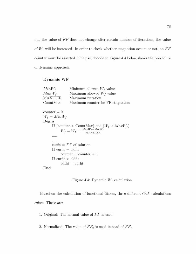
78
i.e., the value of FF does not change after certain number of iterations, the value
of Wf will be increased. In order to check whether stagnation occurs or not, an FF
counter must be asserted. The pseudocode in Figure 4.4 below shows the procedure
of dynamic approach.
Dynamic WF
MinWf Minimum allowed Wf valueMaxWf Maximum allowed Wf valueMAXITER Maximum iterationCountMax Maximum counter for FF stagnation
counter = 0Wf = MinWf
BeginIf (counter > CountMax) and (Wf < MaxWf )
Wf = Wf +MaxWf−MinWf
MAXITER
.....
.....curfit = FF of solutionIf curfit = oldfit
counter = counter + 1If curfit > oldfit
oldfit = curfitEnd
Figure 4.4: Dynamic Wf calculation.
Based on the calculation of functional fitness, three different OvF calculations
exists. These are:
1. Original: The normal value of FF is used.
2. Normalized: The value of FFn is used instead of FF .

79
3. Normalized-Penalized: The value of FFnp is used instead of FF .
With FFnp = FFn − (1− FFn).
Performance evaluation of these three approaches will be carried out in the ex-
periments. Results and discussion will be given in Chapter 6 and 7.
4.6 Concluding Remarks
This chapter and the following chapter are the core of this thesis. In this chapter,
the evolutionary logic design problem has been formulated. The problem statement
and cost function formulation for the proposed algorithm are also detailed. In the
following chapter, the proposed algorithm for ELD based on ACO algorithm will be
discussed.

Chapter 5
ACO ALGORITHM FOR
COMBINATIONAL LOGIC
DESIGN
In Chapter 3, literature review was presented. Problem and cost function formula-
tion have been discussed in Chapter 4. In this chapter, the proposed algorithms for
ACO-based ELD are presented.
5.1 Introduction
A logic circuit can be modelled as a graph of interconnected modules. There exists a
number of possible graphs representing a given circuit. These graphs differ in their
80

81
x
yx
yx
xy
yx +
yx ⊕
zyx
yzx
zxy
zxy ⊕
zyx )( +
))(( zxyyx ⊕+
zxyzyx +⊕ )(zyx )( ⊕
yzx )( ⊕
xzy )( ⊕
Figure 5.1: Figure Illustrating some of the possible paths in function f .
characteristics, i.e., area, delay, and power. As mentioned in the previous chapter,
the number of these graphs could be huge. In this context, the ACO algorithm can
be used as an engine to search the best solution according to a given cost function.
Consider the Boolean function f = xyz + xyz + xyz. This function can be
represented in a number of forms. These representations can be transformed into a
directed acyclic graph G. Figure 5.1 shows some of the possible paths starting from
literal x and ending with two different representations of f .
Using ACO algorithm, the best solution can be found by traversing graph G.
Assume that the objective of the tour construction is to find the shortest path
representing function f . Each ant starts its tour from node x. At each node, the
ant will select the next node to visit. The probability of selecting an edge leading
to a specific node is determined by a pheromone value (τ) and a heuristic value (η)
82
on the edge. The pheromone value implies the preference of search obtained from
knowledge of past generation, while the heuristic value represent the objectives of
optimization process.
When the ant reaches a node with no successor, it will track back and put
additional pheromone on all visited edges. The additional pheromone will in turn
guide the next generation of ants towards preferable solution.
Since the objective is to find the shortest path representing function f , the ant
that finds the path x → (x+y) → (x+y)(xy⊕z) would return the best representation
of function f .
The number of paths shown in Figure 5.1 is more than eleven. The actual
number of paths is large. It is impractical to traverse all those paths. Therefore,
some modifications in ACO algorithm are needed to handle this large search space.
This will be detailed in the next section.
5.2 Modified-ACO (MACO) for Logic Design
In this section, the modified ACO algorithm is presented. It starts with the circuit
encoding, followed by the procedures of the modified ACO algorithms.

83
5.2.1 Circuit Encoding
A circuit is modelled as a matrix M of size n×m. Each cell of the matrix contains a
triplet of attributes consisting of the type of gate used and its corresponding inputs,
i.e., the row indices of the preceding column (see Figure 5.2).
Input 1 Input 2 Gate type
Figure 5.2: Representation of a cell in the matrix.
The value of input 1 and input 2 indicates the row indices from which the current
cell is getting its input from. The value of the gate type indicates the type of the
gate being assigned to that cells assuming a predetermined set of gate types (see
Table 5.1). The input of a gate at position (i, j) can only be connected to the output
of a cell at (i′, (j − 1)) and i′ can be any row index in column (j − 1).
Table 5.1: Gate ID, gate name and output of the gate, considering input a and b.
Gate ID Gate Output
0 WIRE1 a
1 WIRE2 b
2 NOT1 a
3 NOT2 b
4 AND a · b5 OR a + b
6 XOR a⊕ b
7 NAND a · b8 NOR a + b
9 XNOR a⊕ b

84
Figure 5.3: Example of a circuit and its encoding.
Consider the example shown in Figure 5.3. Cell(1,2) whose attribute is (0,3,4)
is an AND gate (according to Table 5.1). The first input of the AND gate of this
cell is connected to the output of cell(0,1), which is a WIRE, and the second input
is connected to the output of cell(2,1).
5.2.2 Modifications of the Ant Colony Algorithm
It is assumed that all ants originate from a dummy cell called nest (see Figure 5.4).
Each ant visits a cell in a column and moves to a cell in the next column, until it
reaches the last column or a cell that has no successor. The idea is to find a correct
and optimal path consisting of logic gates to implement the required truth table and
satisfying the cost function.
Nevertheless, it is possible that the current matrix contains no solution, even
if the size of the matrix is large. In fact, enlarging the matrix will be counter
productive because the time for traversing the paths will exponentially increase.
In order to tackle this problem, the size of the matrix can be kept small enough

85
nest
S(0,0) S(0,1) ...... S(0,m-1)
S(1,0) S(1,1) ...... S(1,m-1)
..... ...... ...... .......
S(n-1,0) S(n-1,1) ...... S(n-1,m-1)
Figure 5.4: Nest cell and matrix M for ant to be traversed.
to reduce the time complexity, but the content of the matrix will be dynamically
changed during the iteration.
At first, the matrix will be randomly filled. After the ants finish their tour, the
solution provided will be evaluated. All cells that are included in the best solution
of the current matrix will be kept. Note that, this solution may not represent the
intended function. All un-needed cells will be removed. These empty cells will be
filled up again in the next iteration. The ants will then traverse the new matrix
and return the best possible solution. If the stopping criteria is not met, the same
procedure will be repeated. Figure 5.5 shows the pseudocode of the approach.
The Filling and Removing cells procedures in MACO algorithm shown in Fig-
ure 5.5 are performed to handle the limitation of ACO algorithm due to the huge
search space of circuit design problem. To further accommodate some improvements
mentioned in Section 3.4, the following modifications are suggested:
1. The Intelligent Ant
2. The Veteran Ant

86
Algorithm Modified ACO (MACO)
BeginFor 0 < i < iteration
F illing the MatrixAnt ActivityRemoving Unfit Cells
EndForEnd
Figure 5.5: Modified ACO algorithm for logic design.
The Intelligent Ant
The original ACO algorithm works on a clearly defined graph where the number of
nodes and/or edges is mostly static and the quality of best solution is unknown. On
the other hand, the result of ELD must be a functionally correct circuit optimized
according to the cost function. While traversing the matrix, each ant must seek
good solution in terms of circuit’s functionality first. Since the length of the tour
is limited by the size of the matrix, the ant should have intelligence to select which
part of its tour that provides the best solution in terms of functional fitness. The
remaining path will be removed from its memory. Using this approach, the ant will
provide better partial solution in every iteration and that the best solution would
emerge at the end of the iterative process.
87
The Veteran Ant
In the original ACO algorithm, all ants will die after finishing their tour. Then, a
new generation of ants is born and use the information of the pheromone trail to
construct their tour. However, if the number of ants is too small to cover all the
existing paths, the quality of new solutions can be worse compared to the old one.
Using larger number of ants will give higher probability of obtaining better or at
least equal solution. However, this will add computation time significantly.
In addition, since the content of the matrix will be dynamically changed, it is
important that the best partial solution is kept in every iteration. This can be
done by saving the paths found by the best ants. Therefore, unlike the original
ACO algorithm, after finishing their tour, some of the best ants will be selected and
upgraded to act as veteran ant (V ant). All ants will die, except the veterans. These
veteran ants will bring their information and ‘lead’ new generation of ants to find
the solution.
For the following reasons, the number of veteran ants used can be more than
one.
1. In order to get the function f = G(f1, f2), both f1 and f2 must be available and
connected through a Boolean operator (a gate) G. If the number of veteran
ants is one, only one partial solution will be saved in each iteration. Both f1
and f2 may be available in the matrix at the same time. Thus, saving f2 as

88
well as f1 (using two veteran ants) will increase the possibility of obtaining
the solution faster.
2. There exist a number of different structural representations for a Boolean
function f . The number of sub-functions of f is even bigger. Finding which
is the best representation for sub-function fk is difficult. Some of the fkican
lead to a good solution, but some of them may lead to a worse solution. Thus,
saving more than one veteran ant can reduce the possibility of getting stuck
in local optimal solutions.
Using more V ants mean more information saved in each iteration. This can
help the search process. However, this can be counter productive since more V ants
means more cells locked during iteration. This will reduce the space for exploring
new solutions. In this thesis, the number of V ant used is two.
As mentioned before, the solution approach has three main steps, namely: filling,
traversing and removing. These three steps will be repeated a number of times until
one of the stopping criteria is met. The details for each of these steps are given in
the following subsections.
5.2.3 Filling the Matrix
The purpose of this step is to fill empty cells in the matrix with randomly generated
attributes. The possible gate type is defined in the gate library. In this procedure,

89
the truth table and functional fitness of the cell will be calculated as well. Figure 5.6
shows the pseudocode of the procedure filling the matrix.
Procedure Filling the Matrix();
/* row maximum number of rows allowed *//* column maximum number of columns allowed */
BeginFor 0 ≤ j < column
For 0 ≤ i < rowIf Cell[i][j] is empty
Cell[i][j].gate = random gate from libraryCell[i][j].input[0] = random integer < rowCell[i][j].input[1] = random integer < rowCalculate truth table();Calculate functional fitness();
EndIfEndFor
EndForEnd
Figure 5.6: Procedure Filling the Matrix.
5.2.4 Ant Activity
The Ant Activity procedure contains three parts: the movement of ants, evaluation
of solutions built and the pheromone update. These are discussed next.

90
Pheromone and Trail Actualization
As mentioned earlier, each ant starts its tour from a dummy cell called nest and
moves to any of the cell in the first column. Next, the ant will move to the second
column, and so on, until it reaches a cell that has no successor. The selection of
which edge to traverse is determined by a stochastic process using Roulette Wheel.
The probability to choose a specific edge depends on pheromone value (τ) and
heuristic value (η) of the edge. The probability of selecting next node is formulated
below [54]:
pkij(t) =
[τij(t)]α · [ηij]
β
∑[τil(t)]α · [ηil]β
(5.1)
The value of α and β imply the preference of the search, whether it depends more
on pheromone value or heuristic value, respectively. Every newly created cell will be
given an initial and small amount of pheromone value. This value will be updated
in every iteration made by the ant.
Heuristic Value (η)
The heuristic value (η) depends on the distance of functional fitness values between
cells, and formulated as follows.

91
d = FFn(i + 1)− FFn(i) (5.2)
η = d + 0.5 (5.3)
The addition of 0.5 in the calculation of η is meant to normalize the value of η
into [0,1]. A decrease in functional fitness means that the value of η is in the range
of [0,0.5), while an increase in functional fitness makes the value of η in the range
of (0.5, 1]
Tour Evaluation
While traversing the matrix, every ant carries information of the paths traversed so
far, e.g., the row index of all cells that were visited. If an ant reaches a cell that
has no successor, it will evaluate and select which part of its tour results in the best
functional fitness value. The value of OF and OvF of the solution will be evaluated.
Pheromone Update
When all ants finished their tour, pheromone update is performed. However, only a
certain number of ‘the best’ ants can update the pheromone along their paths. These
best ants are the V ants mentioned earlier. The pheromone update is performed
using the following:

92
τ(t) = τ(t) + λ ·OvF (t) (5.4)
where OvF (t) denotes the overall fitness of the solution that the ants built and λ is
a constant.
After the pheromone is updated, the pheromone evaporation procedure is per-
formed using the following formula.
τ(t) = (1− ρ)× τ(t), with ρ = (0, 1] (5.5)
In case of multiple outputs circuits, multiple colonies of ants will be used. In this
context, each colony of ants is assigned to find a specific output of the circuit. All
colonies will share the same matrix. The possibility of using the same sub-functions
is established by sharing the pheromone value among different colonies.
5.2.5 Removing the Unfit Cell
After the ants finish their tour, the matrix M will be checked to see which cells are
worth keeping. Each cell can assume two different status, namely l (locked) and r
(removed). The status of a cell is determined by the following rules:
1. A cell is locked if
(a) it is included in the best path

93
(b) it is feeding another locked cell
2. A cell is removed otherwise
The cells that assume r status will be removed at the end of the current iteration.
These empty cells will be then filled up by Filling the Matrix procedure in the
beginning of the next iteration. The example below shows how the algorithm works.
Example 1
Consider, for example, a function f = abc + abc + abc + abc = a ⊕ b ⊕ c. Assume
the first Filling the Matrix is shown in Figure 5.7 (the nest node is not shown).
Let’s take a look at some of the cells in detail. Assume that the initial value of τ is
1, and the value of α = β = 1.
a
b
c
a '
b '
c '
301 (a)
326 (a' c) ⊕
024 (a c )
0 35 (a + a ' )
245 ( c + b ' )
5 41 ( b ' )
308
324
409
149
237
037
0 31
3 4 5
111
425
125
516
432
407
249
540
245
328
550
505
036
332
129
207
Figure 5.7: Result of Filling the Matrix Procedure in the First Iteration for Exam-ple 1.

94
1. Cell (0,0)
This is a primary input whose literal is a. The fitness of the node is 0.5. There
are three edges originating from this node, namely to cell (0,1), cell (2,1) and
cell (3,1). These cells have fitness 0.5, 0,5 and 0.5, respectively. Heuristic
values η for edges to those cells are 0.5 each. Sum of τ 1 × η1 = (1×0.5) +
(1×0.5) + (1×0.5) = 1.5. Recall to Equation 5.1, the values of p for these
edges are:
(a) pcell(0,1) = (1×0.5)/1.5 = 0.33
(b) pcell(2,1) = (1×0.5)/1.5 = 0.33
(c) pcell(3,1) = (1×0.5)/1.5 = 0.33
2. Cell (1,0)
This is a primary input whose literal is b. The fitness of the node is 0.5. There
is one edge originating from this node, namely to cell (5,1). This cell has
fitness 0.5. Heuristic value η for edge is 0.5. Sum of τ 1 × η1 = (1×0.5) =
0.5. Therefore, the value of p for the edge is 1.
3. Cell (0,1)
The node is the result of combination of output from cell(0,0) and cell (3,0)
using WIRE1, which corresponds to literal a. The fitness of the node is 0.5.
There are two edges originating from this node, namely to cell (2,2) and cell
(5,2). These cell have fitness 0.75 and 0.5, respectively. Heuristic values η for

95
these edges are 0.75 and 0.5. Sum of τ 1× η1 = (1×0.75) + (1×0.5) = 1.25.
Then, the value of p for these edges are
(a) pcell(2,2) = (1×0.75)/1.25 = 0.6
(b) pcell(5,2) = (1×0.5)/1.25 = 0.4
4. Cell (5,1)
This is a primary input whose literal is a. The fitness of the node is 0.5. There
is no edge originating from the node. Thus, if an ant visits the node, the tour
of the ant will stop here.
5. Cell (2,2)
The node is the result of combination of output from cell(0,1) and cell (4,1)
using XNOR gate, which corresponds to ((c+b’) ⊕ a). The fitness of the node
is 0.75. There are two edges originating from this node, namely to cell (3,3)
and cell (4,3). Those cell have fitness 0.75 and 0,75 respectively. Heuristic
values η for these edges are 0.75 and 0.75. Sum of τ 1 × η1 = (1×0.75) +
(1×0.75) = 1.5.
The values of p for these edges are
(a) pcell(3,3) = (1×0.75)/1.5 = 0.5
(b) pcell(4,3) = (1×0.75)/1.5 = 0.5

96
Let’s assume that there are two ants that find solutions whose fitness are 0.75.
The paths for these ant are:
1. ant1: fitness = 0.75
path: cell (5,5) → cell (0,4) →cell (2,3) → cell (1,2) → cell (2,1) → cell (4,0)
2. ant2: fitness = 0.75
path: cell (5,5) → cell (0,4) → cell (3,3) → cell (2,2) → cell (0,1) → cell (0,0)
Thus, the new pheromone value for those cells are (assume that λ = 0.5):
1. Pheromone update by ant1
∆τ = λ · f(t) = 0.5 × 0.75 = 0.5 × 0.75 = 0.375
τ(cell (5,5)) = τ(cell (0,4)) = τ(cell (2,3)) = τ(cell (1,2)) = τ(cell (2,1)) =
τ(cell (4,0)) = 1 + 0.375 = 1.375
2. Pheromone update by ant2
∆τ = λ · f(t) = 0.5 × 0.75 = 0.375
τ(cell (5,5)) = τ(cell (0,4)) = 1.375 + 0.375 = 1.75
τ(cell (3,3)) = τ(cell (2,2)) = τ(cell (0,1)) = τ(cell (0,0)) = 1 + 0.375 = 1.375
Note that cells(5,5) and cell(0,4) acquire more pheromones since more ants visit
them in their tour. The pheromone value in each of cell will be:
Note that the bold and underscored values are the cells that were included in the
best tour.

97
1.375 1.375 1.000 1.000 1.75 1.0001.000 1.000 1.375 1.000 1.000 1.0001.000 1.375 1.375 1.375 1.000 1.0001.000 1.000 1.000 1.375 1.000 1.0001.375 1.000 1.000 1.000 1.000 1.0001.000 1.000 1.000 1.000 1.000 1.750
After the pheromone was updated, it will decay using the following rules.
τ =(1 - ρ)× τ , with ρ = (0, 1]
Assume that the value of ρ is 0.8. The pheromone value of each cell will be:
1.100 1.100 0.800 0.800 1.400 0.8000.800 0.800 1.100 0.800 0.800 0.8000.800 1.100 1.100 1.100 0.800 0.8000.800 0.800 0.800 1.100 0.800 0.8001.100 0.800 0.800 0.800 0.800 0.8000.800 0.800 0.800 0.800 0.800 1.400
All cells that are included in the paths of ‘the best ants’ will assume status lock.
In addition, the cell that is feeding a locked cell will be locked. After removal of the
unfit cells, matrix M will consist the cells shown in Figure 5.8.
a
b
c
a'
b'
c'
301 (a)
024 (ac)
035 (a+a')
245 (c+b')
324
401
237
034
111
425
125
432
245
Figure 5.8: Removing of cells in the first iteration.

98
Filling the matrix, second iteration.
All empty cells in the matrix will be filled with randomly generated attributes.
Assume that the result of filling the matrix is shown in Figure 5.9.
a
b
c
a'
b'
c'
301 (a)
126 (b⊕c)
024 (ac)
035 (a+a')
245 (c+b')
248 (c+b')'
100
324
401
154
237
034
026
134
111
425
125
550
432
015
249
056
245
152
018
110
146
252
459
207
Figure 5.9: Filling the matrix in the second iteration
Suppose that there are three ants that found the best solutions.
1. ant1 : fitness = 1
path : Cell (0,0) → cell (0,1) → cell (2,2) → cell (0,3) → cell(3,4)
2. ant2 : fitness = 1
path : Cell (1,0) → cell (1,1) → cell (0,2) → cell (0,3) → cell(3,4)
3. ant3 : fitness = 1
path: Cell (3,0) → cell (3,1) → cell (5,2) → cell (5,3) → cell(3,4)

99
Note that the first two ants are basically building the same circuit. However,
if intelligent ants are used, ant1 and ant2 can stop at cell(0,4) and discard other
succeding cells included in the path. Since ant1 and ant2 requires shorter path
compared to ant3, the solution built will be returned by these two ants.
5.3 Improved-Modified ACO algorithm
Initial experiments showed that some further improvements can be made to increase
the performance of the MACO algorithm. In this section, three modifications are
presented.
5.3.1 Dynamic Search Space
Assuming that the size of the matrix M used to represent the circuit is 5 x 5 and the
interconnection between cells are fixed. Since there are ten types of gates available,
the total number of combination in the matrix M will be 1025. If the interconnections
between cells are made random, this number will increase even bigger. However, if
the size of the matrix M is too small, the search space is limited. Then the quality
of solution obtained may suffer.
In this section, a dynamic search space is proposed. The idea is to have a bigger
search space only when it is required. At the beginning of first iteration, the matrix
is set to its initial size. In the course of any iteration, the size of the matrix may be

100
increased or decreased. Obviously, there should be a limit on the maximum number
of rows and columns of the matrix. It is assumed that the minimum size of the
matrix is NV × NV , with NV as the number of variables of the intended function.
The maximum size of the matrix is (k1 ·NV )× (k2 ·NV ), k1, k2 > 0. Since logic
circuits have a tree-like structure, the number of rows required to implement the
circuits is generally bigger than the number of columns. In other words, k1 > k2.
Row Adjustment
Row Utilization (RU) is defined as the largest ratio of the number of locked cells in
a certain column to the number of rows, or can be formulated as follows:
LC = number of locked cells
RU = max{ LCi
number of row} 0 ≤ i < number of column
Additional row(s) will be introduced if RU is greater than MARU (Maximum Allow-
able Row Utilization). The value of MARU can be determined through experiments.
The setting of 0.75 < MARU < 0.9 were used.
Last Row (LR) is defined as the largest row index of the locked cell in the matrix.
The value of LR will be used to reduce the number of rows in the matrix.

101
Column Adjustment
Column Utilization (CU) is defined as the ratio of the length of best ant’s tour to
the number of columns, or can be formulated as follows:
CU =length of the best path
number of column
Additional column(s) will be introduced if CU is greater than MACU (Maximum
Allowable Column Utilization). The value of MACU can be determined through
experiments.
When the best partial solution is returned, the number of columns will be set
equal to the length of best ant’s tour. The pseudocode in Figure 5.10 explains how
the row and column adjustments are performed in the proposed algorithm.
5.3.2 Perturbation
Perturbation can be performed to further avoid getting stuck in local optimal. The
procedure of perturbation imitates the Selection and Allocation procedures in Simu-
lated Evolution (SE) [15]. First, a goodness measure of each cell is calculated. The
formulation of the goodness measure of a cell is given next.

102
Row and Column Adjustment;/* row number of row *//* column number of column *//* maxrow maximum number of row allowed *//* maxcolumn maximum number of column allowed */
BeginFor 0 < i < iteration
F illing the MatrixAnt Activity
.....If (RU > MARU) and (row < maxrow)
row = row + 1If (CU > MACU) and (column < maxcolumn)
column = column + 1.....
row = LRcolumn = length of the best pathRemoving Unfit Cells
EndForEnd
Figure 5.10: The Use of Row and Column Adjustment.
Goodness Measure
A goodness measure of a cell is determined by a combination of FFns of the cell
and FFns of the neighboring cells, and its position (column) in the current matrix.
Consider cell(i, j) and its surrounding neighbors shown in Figure 5.11. Functional
fitness (FFn) of cell(i, j) is affected by the FFns of its inputs, cell(p1, j − 1) and
cell(p2, j−1) and is affecting the FFn of cell(q, j+1). Thus, the balance of functional
fitness (BFF ) for cell(i, j) is calculated as follows.

103
p1, j-1FF
p2, j-1FF
i, jFF
q, j+1FF
Figure 5.11: How the Neighboring Cells Affect the FFn of Cell(i, j).
P = set of predecessor cells
S = set of successor cells
BFF =∑
k∈P(FFn(i,j)−FFn(k,j−1))+
∑k∈S
(FFn(k,j+1)−FFn(i,j))
Number of neighbors
If FFn of the cells in the first column, i.e., the literals, are assumed to be 0.5
and the FFn(sol) is FFn of the solution, then the expected FFn (EFF ) of cell(i, j)
is equal to:
EFF = 0.5 +(FFn(sol)− 0.5) · jlength of best ant
The goodness of the cell is then calculated as:
G = FFn + BFF
A random number RN is then generated. The maximum value of this random

104
number is set equal to the value of EFF . If G ≥ RN , the cell will be kept.
Perturbation will be performed otherwise.
The move is carried out by replacing the gate type of a cell by a new random
type of gate. The perturbed solution is then evaluated. The perturbed solution
is considered a new solution if its quality, according to the cost function, is better
compared to the original solution.
Perturbation;
Row and Column Adjustment;/* row number of row *//* column number of column *//* M current solution *//* M ′ temporary solution */
BeginM’← MFor 0 ≤ j < column
For 0 ≤ i < rowRN = rand() % ((int) EFF )G = BFF + FFn
If G < RNcell[i][j].gate = assign random gateCalculate truth table cell[i][j]Calculate fitness cell[i][j]
EndIfEndFor
EndForCalculate fitness of M’If M’.fitness > M.fitnessM ← M’
End
Figure 5.12: Perturbation Procedure.

105
a
b
c
d
(a)
a
b
c
d
(b) Figure 5.13: Effect of perturbation on functional fitness value (a) FFn = 0.9375 (b)
FFn = 1.
c
d
a
b
(a)
c
d
a
b
(b) Figure 5.14: Effect of perturbation on objective fitness (a) gate count = 10 (b) gate
count = 8.

106
Perturbation can affect both functional fitness and objective fitness of solutions.
Figure 5.13 shows an example of how perturbation affect the functional fitness. By
changing the circled NAND gate into an XOR gate, the FF of the solution is changed
from 0.9375 into 1. In Figure 5.14, changing the circled OR gate into a WIRE reduce
the number of gate count (area) of the solution. Note that both solutions have the
same FF s.
When the maximum number of iterations is reached, but no functionally correct
circuit is produced, the search process can be continued using the residual function.
This is discussed below.
5.3.3 Residual Function
Given suitable time to evolve, the proposed algorithm could find the target truth
table. However, it could happen that after a given maximum number of iterations,
functionally correct circuits are not produced. In this case, two approaches can be
used, either to have another run of the algorithm, or to extend the search by using
current solution as initial state for the heuristic. No modifications are needed to
perform the first approach. The second approach requires some modifications so
that the extension of the search is performed intelligently. This section addresses
the approach used for extending the search in ELD.

107
Extending the Search
The goal of ELD is to produce functional and optimized circuits. A solution whose
functional fitness is 0.9 is not considered as a good solution. However, in terms of
evolution process, it is 90% functional. Given the time to evolve, it is hoped that by
extending the search into a more directed solution space, the fully functional circuits
can emerge from this solution.
Consider, for example, the target truth table (F ) for the algorithm to be gener-
ated is 10010011. Assume that after maximum iteration is reached, the best solution
returned by the algorithm has the truth table (f1) 10010000. The functional fitness
of the solution is ‘only’ 0.75. Assume that the searching process is continued by
targeting residual truth table (f2) 00000011. Then, if f2 is obtained, both f1 and
f2 can be merged using an OR gate to build the intended truth table F . Since the
search space for f2 is likely to be smaller than the search space for F , the possibility
to find f2 is greater compared to F .
The residual function f2 is obtained by decomposing function F to f1 OR f2.
The decomposition procedure in Boolean algebra allows the use of don’t care values
(*). Thus, the truth table of f2 will be *00*0011. The don’t care values will allow
us to explore richer solution space. In addition to that, the target solutions will
increase, since there are four representations for f2: 00000011, 00010011, 10000011,
and 10010011. This makes the searching process more promising. The procedure of

108
how the decomposition is performed is discussed below.
Decomposition Rules
Decomposition plays an important part in the conventional logic design algorithms.
The idea is to divide a Boolean function into some lower complexity sub-functions, so
that the overall representation can be minimized. Decomposition can be formulated
as follows. Given F as a Boolean function, find f1,...,fk so that F = G(f1, ..., fk),
where G is a Boolean operator (a gate). The sub-functions f1 or fk can be decom-
posed further to obtain simpler functions.
Decomposition can be performed in many ways. Since only two inputs gate are
used, there are three types of decomposition considered, namely: OR, AND and
XOR decomposition. These names denote the gate used for the decomposition.
Thus, decomposition process can be formulated as follows.
Given Boolean function F and known sub-function f1
AND decomposition : find f2 so that F = f1 · f2
OR decomposition : find f2 so that F = f1 + f2
XOR decomposition : find f2 so that F = f1 ⊕ f2
Unfortunately, not all functions can be decomposed using AND or OR decompo-
sition. There is a need of a procedure to check whether a function is decomposable
by AND (OR) decomposition or not. Table 5.2 and Table 5.3 show the value of

109
Table 5.2: AND decomposition table.F f1 f2 Meaning Coding0 0 * don’t care 20 1 0 logic 0 01 0 - can’t happen 31 1 1 logic 1 1
f2 for different input pattern of F and f1 for AND and OR decomposition, respec-
tively. If the value of f2 is ‘-’ (can’t happen condition), then the function F is not
decomposable using f1.
Table 5.3: OR decomposition table.F f1 f2 Meaning Coding0 0 0 logic 0 00 1 - can’t happen 31 0 1 logic 1 11 1 * don’t care 2
In contrast with the AND and OR decomposition, function f2 can always be
produced by decomposing F to f1 by XOR decomposition, since f2 = F ⊕ f1.
However, in XOR decomposition, the f2 will be in the form of completely specified
functions, i.e., the truth table of f2 does not have don’t cares values, as shown in
Table 5.4. Thus, it is possible that f2 is more complex than f1 (or F ) itself.
Merging the solutions
Using the concept of residual function, the algorithm will work in at least two
stages. The first stage is to find f1, while the second one is to find f2. At the end
of the second stage, f1 and f2 will be merged to obtain a new solution. Consider,

110
Table 5.4: XOR decomposition table.F f1 f2 Meaning Coding0 0 0 logic 0 00 1 1 logic 1 11 0 1 logic 1 11 1 0 logic 0 0
for example, a function F with truth table 1000111111100101. Assume that the
first stage of the algorithm found f1 whose truth table is 0000111110100101 (see
Figure 5.15 (a)). Assume that OR decomposition is used. Using OR decomposition
table, truth table of f2 is then 1000*****1*00*0*. Assumed that the second stage of
the algorithm find f2 with truth table 1000001001000001, shown in Figure 5.15 (b).
With OR gate as operator, the function F ′ obtained from merging f1 and f2 is shown
in Figure 5.15 (c).
If F ′ = F , it means that the algorithm found the functionally correct circuits.
However, it is possible that f2 was not found and F ′ 6= F . In this case, another
stage of decomposition must be performed. The new f2 will be calculated by using
F ′ as f1. This process is continued until the maximum number of decomposition
da'
b'
d'a
c'b
(a)
(b)
d'a
c'
da'
b'
b
F
1f
2f
(c)
merging
decompositionoperator
Figure 5.15: Example of using the residual function.

111
Decomposition()
If (s = 0) and (solution.FF = 1)Return solution
ElseIf (s > 0)
Merge(f1, f2, G, F ′)If (F ′ = F )
Return solutionEndIf
f1 ← solutionIf (s = 0)
G = OR gateElseIf (s = 1)
G = AND gateElse
If Check decompose(F , f1, OR) > 0G = OR gate
ElseIf Check decompose(F , f1, AND) > 0G = AND gate
Else G = XOR gateEndIf
Decompose(F , f1, G, f2)
EndIf
Figure 5.16: Decomposition procedure.

112
stages allowed is reached.
In order to get the benefit of the don’t care values, both of AND and OR decom-
position get higher priority compared to the XOR decomposition. The justification
is that the unneeded minterms from f1 can be removed using AND decomposition
and the required minterms can be added using the OR decomposition. Note that the
“can’t happen” condition will be treated as normal don’t cares. If both decomposi-
tions fail, the XOR decomposition is performed. Figure 5.16 shows the pseudocode
of decomposition procedure.
Improved Modified ACO (IMACO) algorithm
/* MAXITER Maximum iteration *//* MAXSTAGE Maximum decomposition stage */
For 0 < s < MAXSTAGEFor 0 < i < MAXITER
Filling the Matrix();Ant Activity();Removing Unfit Cells();Perturbation();
EndDecomposition();
EndReturn best solution
End
Figure 5.17: Improved-Modified ACO algorithm for logic design.
113
Putting It All Together
Having the perturbation and decomposition procedures incorporated, the improved
modified ACO (IMACO) algorithm for logic design is presented in Figure 5.17.
The IMACO algorithm is more complex compared to the previous one (see Fig-
ure 5.5). However, the probability of obtaining better quality result is higher. Ex-
perimental results and comparison between the proposed algorithms will be given
in the next chapter.
5.4 Concluding Remarks
In this chapter, a Modified Ant Colony Optimization (MACO) algorithm for the
design of digital logic circuits is introduced. The need for a modification to the
original ACO algorithm is discussed. Moreover, an improved version of the MACO
algorithm that includes the use of perturbation and residual function is also pro-
posed. In the next chapter, performance evaluation, experiments and results of the
proposed algorithm are presented.

Chapter 6
EXPERIMENTS AND RESULTS
This chapter and the following one are dedicated to experiments and results obtained
from applying the proposed algorithms. This chapter concentrates on the evaluation
of different possible schemes, while the next chapter will present comparison with
existing techniques.
6.1 Experimental Setup
A number of procedures needed for conducting the experiments are first introduced.
This includes the setting of inputs, tools and parameters.
Input: In order to perform the experiments, some benchmark circuits are used as
test cases. The benchmark consists of twenty randomly generated truth tables of
different complexity in addition to twelve circuits obtained from ISCAS’85 bench-
114

115
mark. All circuits are in PLA format. Using this format, the proposed algorithm
can accept don’t care inputs as mentioned in Section 3.4. Details of these circuits
are given in Appendix A. Table 6.1 shows a summary of these circuits.
Table 6.1: Summary of circuits used for the experiments.Single Output Multiple OutputCircuits
Number ofSpecification
Number ofSpecification
Notesusedcircuits circuits
Random 20Number of
- - -inputs: 2 - 6Number of Number of arithmetic circuits:inputs: 3 - 7 inputs: 3-7 majority, parity,ISCAS’85 3 9
Number of adder and multiplieroutputs: 2-10
Technology parameters used in the experiments is obtained from MOSIS 0.25 µ
library [80]. These parameters are written into a text file using a certain format.
This can be seen in Appendix A.
Parameters for the Algorithm: Performance of iterative heuristics depends on
the fine-tuning of its parameters. Otherwise mentioned explicitly, in general, these
parameters listed below are used. Note that NV is the number of variables for a
specific circuit.
• α = 1
• β = 1
• ρ = 0.1
• Number of ants = 10 * NV
• Number of generations = 2 * NV
• Maximum number of iterations = 500 * NV

116
• Number of runs = 20
• Minimum size of the matrix = NV ×NV
• Maximum size of the matrix = (k1 ·NV )× (k2 ·NV ), 2 ≤ k2 < k1
• Maximum number of decomposition stages = 6
Four types of experiments are carried out to measure the performance of the
proposed algorithms. These include experiments for different fitness function calcu-
lation, effect of dynamic search space, effect of perturbation and decomposition, and
different optimization objectives. The quality of solutions are measured according
to the area, delay and power of the circuits. These metrics are measured in µm2, ps
and pW units, respectively.
6.2 Performance of Different Fitness Calculation
The objective of this experiment is to know which fitness function calculation works
best for the proposed algorithms. This includes the selection of weighting scheme
and calculation of FF .
6.2.1 Effect of Different Weighting Scheme
As mentioned in Chapter 4, two approaches can be used to select the value of WF ,
namely: static and dynamic. These are examined below.
For the purpose of this experiment, the size of the matrix is set as (2 · NV ) ×
(2 · NV ). The circuits used as test cases are those having four or five inputs. In

117
addition to the quality of results in terms of cost function, a measure called design
rate is used for comparison. Design rate is defined as the percentage of functionally
correct circuits delivered by the algorithm from the whole runs of experiment using
a given maximum number of iterations.
Table 6.2, Table 6.3 and Table 6.4 show the experimental results, assuming the
value of WF is 0.5, 0.75 and 0.875, respectively.
Table 6.2: Experimental results for WF = 0.5.
Circuit design rateBest result
Area Delay Powercircuit1 55 15066 5.94 6.572circuit2 70 15066 5.94 6.572circuit3 45 10692 3.05 3.818circuit4 100 1458 0.01 0.666circuit5 25 12150 3.90 5.076circuit6 55 10935 3.34 3.818circuit7 60 12393 6.66 4.732circuit8 100 7290 2.96 3.161circuit9 0 - - -circuit10 5 12393 5.32 4.483
Table 6.3: Experimental results for WF = 0.75.
Circuit design rateBest result
Area Delay Powercircuit1 100 14823 5.89 6.57circuit2 100 14823 5.89 6.57circuit3 70 11421 3.35 3.82circuit4 95 1458 0.01 0.67circuit5 85 12150 3.90 5.08circuit6 100 10935 3.34 3.82circuit7 85 12636 6.66 4.73circuit8 100 7290 2.96 3.16circuit9 65 17496 5.42 5.27circuit10 35 12393 5.32 4.48

118
Table 6.4: Experimental results for WF = 0.875.
Circuit design rateBest result
Area Delay Powercircuit1 100 14094 5.55 5.28circuit2 95 14823 5.89 6.57circuit3 85 10692 3.05 3.82circuit4 90 1458 0.01 0.67circuit5 85 12150 3.90 5.08circuit6 100 10935 3.34 3.82circuit7 100 12393 6.27 4.48circuit8 100 7290 2.96 3.16circuit9 80 16038 6.00 5.27circuit10 25 12393 5.32 4.48
It was expected that the setting of WF equal to 0.5 will give the best solution in
both FF and OF . However, this happened to be a wrong assumption. Indeed, the
setting of WF = 0.5 is the worst among the others. The average design rate for this
setting is only 51.5%, which is quite low. It gives 100% design rate only for small
circuits (circuit4 and circuit8) and even fails to deliver working circuit for circuit9.
The reason behind this is that the algorithm was trying to satisfy both FF and OF
at the same time during the course of iteration. It is more difficult for the algorithm
to move to a new solution with higher FF if its OF is low. Thus, the algorithm will
spend more time with solutions that have low FF value, which in turn reduces the
possibility of delivering correct circuits.
In terms of design rate, both the setting of WF = 0.75 and WF = 0.875 are
much better compared to WF = 0.5. The average design rate is 82.5% and 86%
respectively. In terms of OF , the setting of WF = 0.875 gives the best results

119
compared to other settings. This happens because the algorithm reached the solution
having FF equal to 1 in the early stages of iteration.
The highest value that can be assigned to WF is equal to MAXWF = LL + 1
,
with L is the length of the truth table. The proof is the following.
The overal fitness function (see Equation 4.13) can be rewritten as.
OvF ∗ (M + N) = FF ∗M + OF ∗N (6.1)
Note that FF and OF are fractions in [0, 1], with
FF =H
L
where H is the number of hits and L is the length of the truth table.
If M is set equal to L, the first term in Equation 6.1 will be equal to H, which
is a decimal number. By setting N equal to 1, the second term in Equation 6.1
will stay as a fraction. Since the value of M determines the importance of FF in
contrast to OF , the ratio of M to N is equal to L : 1. Setting M equal to a value
larger than L will not give any effect since the second term of Equation 6.1 is already
a fraction. The value of MAXWF is then
M
M + N=
L
L + 1

120
If the value of WF is increased, the importance of OF will decrease. Consider,
for example, the use of MAXWF as WF . During the iterations, solutions that
have higher number of matching truth table will be taken, regardless of the value
of OF . The value of OF will be considered if there exist two solutions having the
same value of FF . In this case, the solution having higher OF will be considered.
Table 6.5: Experimental results for dynamic WF .
Circuit design rateBest result
Area Delay Powercircuit1 90 14823 5.89 6.57circuit2 95 15066 5.94 6.57circuit3 50 10692 3.05 3.82circuit4 90 1458 0.01 0.67circuit5 75 12150 3.90 5.08circuit6 95 10935 3.34 3.82circuit7 100 12393 5.05 4.38circuit8 100 7290 2.96 3.16circuit9 55 15066 5.42 5.27circuit10 25 12393 5.32 4.48
For small circuits, it is better to use higher WF values as shown in Table 6.2,
Table 6.3 and Table 6.4. However, for larger circuits, the use of higher WF values
can be counter productive. Because, it may happen that a solution having high FF
with low OF value is obtained. However, low OF value means less in satisfying the
objectives, i.e., the solution may have large area, or delay, or power. Consider, for
example, in the case of larger area. The solution will require quite a number of cells
to be locked during the iterations. If this happened quite often, it will be difficult
for the algorithm to escape local optimal because the number of empty cells in the

121
matrix to explore new solution space will be less. An answer for this problem is the
use of dynamic WF (see Chapter 4).
The experimental results for dynamic WF is shown in Table 6.5. For the purpose
of the experiment, a minimum WF value is set equal to 0.5 while the maximum value
is set to 0.9. As can be seen from the table, the design rate of this approach is lower
compared to the one with WF = 0.875. In terms of OF , the use of dynamic WF
leads to worse or similar results for small circuits, i.e., circuit1 to circuit8. However,
as the size of the circuits is increased, i.e., circuit9, the use of dynamic WF leads
to results that are better compared to those obtained using static WF .
6.2.2 Effect of Different FF Calculations
Using dynamic WF , performance of different functional fitness calculations is car-
ried out using larger circuits. Recall to Chapter 4, there are three types of func-
tional fitness calculations considered, original (FF ), normalized FF (FFn), and
normalized-penalized FF (FFnp). Table 6.6 shows results of the experiments.
The original FF calculation suffers a lot for larger circuits. It fails to deliver
working circuits for three out of seven cases. The normalized FF (FFn) also fails
for those same circuits. However, the design rate for FFn is better compared to FF .
This is due to the ‘normalization’ done to the calculation of FF . By normalizing
FF , the algorithm will find both the intended Boolean function and the inverted
Boolean function. Whichever comes first will be considered.

122
Although it fails to deliver working circuits for circuit12, the normalized-penalized
FF (FFnp) is the best compared to the other two. Note that, circuit12 is one ex-
ample that needs to be highlighted since the size of the circuit is quite large. It
will be shown later that this circuit can be generated using the concept of residual
functions.
Table 6.6: Results obtained for different FF calculations.
CircuitDesign Rate
Original FF Normalized (FFn) Normalized-penalized (FFnp)circuit9 55 60 80circuit10 25 45 40circuit11 10 20 55circuit12 0 0 0circuit13 25 55 50circuit14 0 0 20circuit15 0 0 25
From this time onward, except if it is mentioned explicitly, the experiments will
be carried out using dynamic WF with FFnp.
6.3 Dynamic Search Space
The purpose of this experiment is to show how the use of dynamic matrix size affects
the performance of the proposed algorithm. Table 6.7 shows a comparison in terms
of design rate and execution time for both static matrix size (SM) and dynamic
matrix size (DM) approaches.
In terms of design rate, DM clearly outperforms SM . In addition to that,

123
circuit12 that was not generated using SM was delivered by DM . In terms of
execution time, DM was superior compared to SM for small circuits (circuit1 to
circuit8) by up to 25% time saving. Note that both approaches use the same number
of iterations. The difference in execution times is caused by the different sizes of
the search space explored by both approaches. For bigger circuits, DM provides
faster execution time for circuit9 and circuit10, with 37.5% and 42.5% time saving
as compared to the ones obtained using the SM . For the remaining circuits, SM
requires less computation time compared to DM . Consider the case of circuit13.
The execution time of DM is three times higher compared to the one for SM .
For this circuit, it was observed that the algorithm can achieve solutions having
FF equal to 0.969 in a very short time. However, it was very difficult to obtain
solutions higher FF value. Therefore, the design rate for the circuits is low in SM .
On the other hand, when local optima is observed, DM will increase the size of the
matrix. This will in turn increase the execution time of the algorithm. However, the
probability of obtaining functionally correct circuits will increase. In other words,
the design rate of DM is higher as compared to the one of SM .
Table 6.8 shows a comparison of quality of solutions in terms of area obtained
using SM and DM . Except for circuit12, DM provides better circuits in six out
of fourteen cases, with 1% to 13% reduction in area. Both approaches produce the
same quality of circuits in the remaining cases.
For large circuits, i.e., circuit9 to circuit15, except for circuit14, DM produces

124
Table 6.7: Experimental result for static and dynamic matrix in terms of design rateand computation time.
Circuitdesign rate timeSM DM SM DM
circuit1 100 100 21.00 15.27circuit2 100 100 20.95 15.30circuit3 100 100 21.10 14.53circuit4 100 100 4.30 3.50circuit5 100 100 20.60 17.03circuit6 100 100 20.70 14.80circuit7 100 100 21.10 16.27circuit8 100 100 21.15 12.90circuit9 80 100 131.44 82.13circuit10 40 100 134.13 77.07circuit11 55 93 39.36 57.63circuit12 0 13 - 151.50circuit13 50 100 39.20 121.43circuit14 20 87 132.75 208.13circuit15 25 93 132.60 188.64
Table 6.8: Area result obtained using static and dynamic matrix size.Circuit SM DM Ratiocircuit1 14823 12879 0.87circuit2 14823 13122 0.89circuit3 10692 10692 1.00circuit4 1458 1458 1.00circuit5 12150 13365 1.10circuit6 10935 10935 1.00circuit7 12150 12393 1.02circuit8 7290 7290 1.00circuit9 15066 15066 1.00circuit10 12393 11178 0.90circuit11 17739 17496 0.99circuit12 0 45684 ∼circuit13 20169 19683 0.98circuit14 22842 26730 1.17circuit15 21870 20655 0.94

125
better or equal quality results compared to SM . In circuit14, the area of the ob-
tained circuit using DM is higher compared the one obtained using SM . However,
the design rate of SM for this circuit is 20% compared to 87% using DM . In other
words, compared to SM , DM has much higher probability of arriving at solutions.
6.4 Residual Function
The MACO algorithm depicted in Figure 5.5 failed to deliver some large circuits,
i.e., circuit18 up to circuit20. The use of residual function, as included in IMACO
algorithm (see Figure 5.17), for these circuits is found necessary. Table 6.9 shows
experimental results for these circuits considering residual function. Note that cir-
cuit12 is added in addition to those of large circuits since this circuit is one of the
hard to implement circuits as indicated in the previous sections.
Table 6.9: Results obtained using IMACO algorithm.
Circuit design rateBest result Average result
timeArea Delay Power Area Delay Powercircuit12 70 45684 14.30 17.36 83891.08 21.80 28.51 1920.85circuit18 55 63666 23.83 22.01 81162.00 26.09 26.85 1046.70circuit19 50 54432 11.34 19.68 78570.00 21.14 25.56 1241.50circuit20 55 60264 12.43 20.23 73483.20 23.78 25.68 1016.00
As can be seen from the table, all considered circuits in the experiment were
delivered by the algorithm. In addition, an improvement in the design rate for
circuit12 was observed. The design rate for this circuit is 70%, as compared to
13% in the previous experiment (see Table 6.7). However, as has been expected,

126
the execution time for IMACO algorithm is increased tremendously. The execution
time of IMACO algorithm is up to 5 times as compared to the MACO algorithm.
6.5 Different Optimization Objectives
The cost function considered in this work includes area, delay and power consump-
tion of the circuits. Three sets of experiments are performed. These are:
1. Area optimization with delay and power as constraints (AODPC)
2. Delay optimization with area and power as constraints (DOAPC)
3. Power optimization with area and delay as constraints (POADC)
Basically, since fuzzy logic is used to aggregate the cost functions, the algorithm
will try to find solutions that are optimized for area, delay and power at the same
time. The term constraints used above is used to imply that the solutions obtained
must have area (delay or power) less than or equal to the stated maximum value.
AODPC
In order to understand how the optimization is performed, it is important to observe
the behavior of the proposed algorithms during the course of experiments. Figure 6.1
shows the behavior of OvF , FF and OF (overall fitness, functional fitness and
objective fitness) against time during one of the experiment performed for circuit1.

127
As can be seen from the figure, the value of FF increases with time. Since the
circuit is relatively small in size, the functionally correct circuit (FF equal to one)
is found in less than 50 iterations. In contrast with FF , the value of OvF will never
be one, unless if the circuit contain only wires. In fact, the value of OvF depends
on the value of FF and OF .
The value of OF may increase or decrease during the course of iterations. Fig-
ure 6.2 shows the behavior of fitness function for the first 50 iterations. As can be
seen from the figure, at about iteration number 25, the value of OF was decreas-
ing. However, the value of FF is increasing. As mentioned in the previous chapter,
whenever solution with higher FF value is obtained, the move to the new solution
is preferable. However, if there is no increase in FF , optimization in OF will be
carried out.
The optimization of OF is performed according the fuzzy rule applied in the
experiment. Figure 6.3 and Figure 6.4 show the behavior of OF during the first 50
iterations and 150 iterations, respectively. The value of area, delay and power are
normalized to the highest value achieved during the iterations.
As can be seen from Figure 6.3, the value of OF at iteration number 40 reaches
its lowest value because the value of area, delay and power reach their largest value
at the same time. However, after iteration number 40, the value of OF is increasing
(see Figure 6.3 and Figure 6.4). This means that the optimization in terms of
objective functions is performed.

128
0.2
0.4
0.6
0.8
1
0 200 400 600 800 1000 1200 1400 1600 1800
FF OvF OF
Figure 6.1: Behavior of functional fitness function for circuit1 in the first 2000iterations using AODPC.
0
0.2
0.4
0.6
0.8
1
1.2
0 10 20 30 40 50
FF OvF OF
Figure 6.2: Behavior of functional fitness function for circuit1 in the first 50 itera-tions using AODPC.

129
0
0.2
0.4
0.6
0.8
1
0 10 20 30 40 50
OF Area Delay Power
Figure 6.3: Behavior of objective fitness function for circuit1 in the first 50 iterationsusing AODPC.
0.4
0.5
0.6
0.7
0.8
50 60 70 80 90 100 110 120 130 140 150 160 170 180 190 200
OF Area Delay Power
Figure 6.4: Behavior of objective fitness function for circuit1 in iteration 50 toiteration 200 using AODPC

130
In AODPC, it is expected that the circuits obtained will have less area as com-
pared to the ones produced by other set of experiments. Figure 6.4 illustrates this
behavior. As can be seen in the figure, at about iteration number 140, new solution
with less area is accepted although it has higher delay compared to the old solution.
Table 6.10: Results of different optimization objectives.
CircuitAODPC DOAPC POADC
area delay power area delay power area delay powercircuit10 11178 5.42 4.06 12393 5.32 4.48 11178 5.42 4.06circuit11 17253 5.91 7.22 22599 5.61 9.30 18225 6.29 6.95circuit12 45684 14.30 17.36 57591 13.88 20.56 45684 14.30 17.36circuit18 63666 23.83 22.01 77760 16.68 28.75 64638 20.04 21.09majority 13851 4.57 5.06 16038 4.19 5.02 14580 4.53 4.72xor8 20655 5.90 9.32 20655 5.90 9.32 20655 5.90 9.32xor9 23328 8.84 10.65 27216 8.84 11.48 23814 9.57 10.65add2 24300 11.48 9.96 31347 8.96 11.46 25029 13.30 9.57add3 49086 21.96 18.47 53703 12.98 21.48 54675 14.36 20.55mul2 12636 3.56 4.66 18225 2.96 5.99 14823 4.44 4.66mul3 59292 15.03 17.54 74358 13.14 21.65 73386 16.33 19.11con1 38151 6.70 13.74 38394 6.24 12.65 42282 9.79 13.97
The results of the experiments for a number of selected circuits are shown in
Table 6.10. The table shows the value of area, delay and power for the best solution
obtained by different set of experiments. In order to measure the performance of
the algorithm for different objectives, the results in this table are normalized with
respect to the results of AODPC experiment.

131
DOAPC
Table 6.11 shows the normalized value of DOAPC. As can be seen from this table, the
percentage of improvement in delay varies. The improvement is, however, mostly
accompanied by additional area and power consumption. Figure 6.5 shows the
normalized area, delay and power for DOAPC. As can be seen in the figure, the
value of normalized delay is always less than one. It means that for the given single-
output circuits, DOAPC provides circuits with better or at least the same delay as
compared to the ones produced by AODPC.
Table 6.11: Results of DOAPC experiments normalized with respect to results ofAODPC.
Circuit Area Delay Power % area % delay % powercircuit10 1.11 0.98 1.10 -10.87 1.79 -10.36circuit11 1.31 0.95 1.29 -30.99 5.01 -28.84circuit12 1.26 0.97 1.18 -26.06 2.97 -18.42circuit18 1.22 0.70 1.31 -22.14 30.02 -30.62majority 1.16 0.92 0.99 -15.79 8.29 0.69xor8 1.00 1.00 1.00 0.00 0.00 0.00xor9 1.17 1.00 1.08 -16.67 0.00 -7.83add2 1.29 0.78 1.15 -29.00 21.98 -15.07add3 1.09 0.59 1.16 -9.41 40.90 -16.29mul2 1.44 0.83 1.29 -44.23 16.76 -28.56mul3 1.25 0.87 1.23 -25.41 12.59 -23.40con1 1.01 0.93 0.92 -0.64 6.82 7.91
For multiple output circuits, i.e., the longest delay appear in the circuits is
considered (see Table 6.10). Figure 6.6 shows the normalized area, delay and power
for multiple output circuits. It is observed that the value of normalized delay is
always less than one. In general, DOAPC has performed its objective by producing
circuits with better delay as compared to the one produced by AODPC.

132
0.0
0.2
0.4
0.6
0.8
1.0
1.2
1.4
1.6
circuit10 circuit11 circuit12 circuit18 majority xor8 xor9
Area Delay Power
Figure 6.5: Normalized results of DOAPC for single output circuits.
0.0
0.2
0.4
0.6
0.8
1.0
1.2
1.4
1.6
1.8
add2 add3 mul2 mul3 con1
Area Delay Power
Figure 6.6: Normalized results of DOAPC for multiple output circuits.

133
POADC
Table 6.12 shows the normalized value of POADC. As can be seen, the percentage of
improvement for power is less compared to the percentage of improvement for delay
in DOAPC. Figure 6.7 shows the normalized area, delay and power in POADC for
single output circuits. It is observed that the value of normalized power for these
circuits are less or at least equal to one, which means the optimization of power is
achieved.
Table 6.12: Results of POADC experiments normalized with respect to results ofAODPC.
Circuit Area Delay Power % area % delay % powercircuit10 1.00 1.00 1.00 0.00 0.00 0.00circuit11 1.06 1.06 0.96 -5.63 -6.36 3.73circuit12 1.00 1.00 1.00 0.00 0.00 0.00circuit18 1.02 0.84 0.96 -1.53 15.94 4.20majority 1.05 0.99 0.93 -5.26 0.88 6.59xor8 1.00 1.00 1.00 0.00 0.00 0.00xor9 1.02 1.08 1.00 -2.08 -8.24 0.00add2 1.03 1.16 0.96 -3.00 -15.86 3.96add3 1.11 0.65 1.11 -11.39 34.62 -11.24mul2 1.17 1.25 1.00 -17.31 -24.54 0.00mul3 1.24 1.09 1.09 -23.77 -8.66 -8.92con1 1.11 1.46 1.02 -10.83 -46.12 -1.64
Figure 6.8 shows the normalized area, delay and power for multiple output cir-
cuits. The figure shows some discouraging results. Improvement in power are ob-
served for add2 (2-bit adder) and mul2 (2-bit multiplier) circuits. POADC however,
failed to produce circuits with better power consumption in contrast to AODPC.

134
0.0
0.2
0.4
0.6
0.8
1.0
1.2
1.4
circuit10 circuit11 circuit12 circuit18 majority xor8 xor9
Area Delay Power
Figure 6.7: Normalized results of POADC for single output circuits.
0.0
0.2
0.4
0.6
0.8
1.0
1.2
1.4
1.6
1.8
add2 add3 mul2 mul3 con1
Area Delay Power
Figure 6.8: Normalized results of POADC for multiple output circuits.

135
From the three sets of experiments it was observed that the performance of
POADC is the worst. There is no much improvement in power consumption as
expected. The reason behind this behavior is twofold:
1. By using OWA operator of fuzzy logic, the optimization of area, delay and
power are performed at the same time.
2. Power consumption of a given circuit is proportional to the number of gates
it has. Thus, in agreement with point 1, the quality of obtained circuits in
POADC are generally the same with the ones produced by AODPC.
6.6 Concluding Remarks
In this chapter, performance of the solution approach was evaluated. It began with
the performance of different fitness function calculations and continued with the
dynamic search space and improved-modified ACO algorithm. The approach was
able to arrive at acceptable solutions in all test cases. The performance of different
set of experiments has also been presented. Comparison of the solution approach
with the existing technique is presented in the next chapter.

Chapter 7
COMPARISON WITH
EXISTING TECHNIQUES
In this chapter, a comparison of the results obtained using the introduced techniques
is presented.
7.1 Comparison with Existing ACO-based Tech-
nique
In this section, the results of our experiments are compared to the results obtained
from the existing ACO-based technique proposed by Coello [6]. Since this technique
tries to minimize the use of gate count only, the comparison is performed using the
results of AODPC of the proposed algorithm. This includes comparison in terms of
136

137
Table 7.1: Comparison with Coello [6] in terms of design rate.Circuit Coello [6] MACOcircuit1 70 100circuit2 70 100circuit3 90 100circuit4 100 100circuit5 30 100circuit6 100 100circuit7 50 100circuit8 100 100mul2 100 100
design rate, quality of results and performance of the algorithm.
7.1.1 Comparison of Design Rate
Table 7.1 shows comparison of both Coello’s [6] technique and the proposed algo-
rithm in terms of design rate. For this purpose, the same test cases were used. It
should be noted that the technique described in [6] failed to deliver any valid results
for large single-output circuits.
Since the test cases are relatively small, the MACO algorithm is used. As can
be seen from Table 7.1, the MACO algorithm outperformed the existing ACO-based
technique in terms of design rate. The average design rate for MACO algorithm is
100% as compared to 78.89% for Coello [6].

138
7.1.2 Comparison of the Quality of Solutions
Table 7.2 shows a comparison of the quality of solutions in terms of gate count,
area, delay and power consumption as a result of using both techniques. The table
shows that there are significant improvements in terms of area for all cases, except
for circuit4 that contains a single gate only. The highest improvement is obtained
in circuit5, which is 60.98%. Except for circuit7 and mul2, the solutions provided
by MACO are better in terms of delay and power. In addition to that, although
AODPC is targeting area minimization, some improvements in terms of gate count
are also observed.
0.0
0.2
0.4
0.6
0.8
1.0
1.2
1.4
1.6
circuit1 circuit2 circuit3 circuit4 circuit5 circuit6 circuit7 circuit8 mul2
Gate count Area Delay Power
Figure 7.1: Results of MACO normalized with respect to Coello [6].
Figure 7.1 shows the results of MACO algorithm for the given test cases. Note
that the results are normalized with respect to Coello’s [6] technique. It can be seen
that the normalized area for these circuits are always ≤ 1 which means that the
obtained circuits require less area compared to the ones produced by Coello’s [6].

139
Tab
le7.2:
Com
parison
with
Coello
[6]in
terms
ofarea,
delay
and
pow
er.
Coello
[6]M
AC
O%
Improvem
entC
ircuitG
atecount
Area
Delay
Pow
erG
ateC
ountA
reaD
elayPow
erG
ateC
ountA
reaD
elayPow
er
circuit16
167677.36
6.577
128795.57
4.97-16.67
23.1924.34
24.33
circuit26
167677.36
6.577
131225.18
5.28-16.67
21.7429.55
19.60
circuit36
148234.22
5.247
106923.05
3.82-16.67
27.8727.83
27.17
circuit41
14580.01
0.671
14580.01
0.670.00
0.000.00
0.00
circuit514
2988912.81
8.096
116645.57
5.0857.14
60.9856.55
37.26
circuit65
133653.37
4.917
109353.34
3.82-40.00
18.180.98
22.21
circuit79
189544.53
3.397
123935.59
4.3722.22
34.62-23.37
-28.79
circuit83
77763.69
3.163
72902.96
3.160.00
6.2519.78
0.03
mul2
717253
2.973.82
712636
3.564.66
0.0026.76
-19.78-22.05

140
a
b
c
d
out0
out3
out1
out2
Figure 7.2: 2-bit Multiplier obtained by Coello [6].
a
b
c
d
out0
out2
out1
out3
Figure 7.3: 2-bit Multiplier obtained by MACO.
Case study: 2-bit multiplier
Figure 7.2 and Figure 7.3 show the 2-bit multiplier circuits obtained from Coello [6]
and MACO respectively. Each circuit consist of seven gates. However, as can
be seen from the figures, MACO results in the use of NAND and NOR gates in
contrast to AND and XOR gates. Since both NAND and NOR gates requires less
area, the circuits obtained by MACO has less area in contrast to the one produced
by Coello [6]. In addition, as can be seen in Figure 7.2, output out2 of the circuit

141
has the longest delay, i.e., the level of out2 is 3. However, the highest level in the
circuit produced by MACO is 2. Thus, delay of the circuit produced by MACO will
be less than the one produced by Coello [6].
7.1.3 Comparison of Execution Time
Here comparison of execution time for both techniques is conducted. The experi-
ments were carried out using P4 2GHz CPU, 512 MB RAM. Although the length
of execution time depends on some variables such as the number of iterations, size
of the matrix and the number of gate types, comparison is performed in order to
contrast the performance of both techniques.
Table 7.3 shows the average execution time for the given test cases. It is shown
that for single-output circuits (except circuit4), MACO results in a saving of more
than 70% in execution time. Since circuit4 requires only one gate, the deterministic-
like approach of [6] provides faster execution time in contrast to MACO. In addition
to that, Coello’s approach is worse when it comes to multiple-output circuits. As can
be seen in the case of mul2 circuit, MACO saves 98% execution time as compared
to [6].

142
Table 7.3: Comparison with Coello [6] in terms of execution time.Circuit Coello [6] MACO % timecircuit1 61.43 15.27 75.15circuit2 61.43 15.17 75.31circuit3 49.70 14.67 70.49circuit4 0.40 3.50 -775.00circuit5 76.00 16.97 77.68circuit6 50.70 14.83 70.74circuit7 75.60 16.10 78.70circuit8 50.40 12.70 74.80mul2 2876.29 57.20 98.01
7.2 Comparison with Existing Conventional Tech-
niques
In this section, comparison of the proposed algorithm with an existing conventional
technique is given. For this purpose, SIS tools are used. However, SIS does not
consider load capacitance in their delay calculation and does not consider power
optimization. Therefore, the results obtained from SIS are in the form of netlist files.
These netlist files will be used as input to the cost function calculation procedures
of the proposed algorithm to determine the area, delay and power of the circuits
obtained.

143
Area Optimization
In order to compare the performance of the proposed algorithm based on area op-
timization, AODPC experiment was performed. The results from SIS are the area
optimized circuits obtained by executing rugged.script, mapped for area minimiza-
tion. Both SIS and the proposed algorithm use the same gate library.
Since the circuits used as test cases are large circuits, the results obtained using
IMACO algorithm are considered. Table 7.4 shows the results for single-output
circuits using both techniques. The table shows that except for circuit20, IMACO
produces circuits with lesser area than SIS. The highest improvements are obtained
for 8-bit and 9-bit odd parity circuits. Parity circuits are best implemented using
XOR (XNOR) gates. Unfortunately, SIS is unable to perform XOR decomposition.
Thus, the parity circuits obtained by SIS will require larger area as compared to the
ones obtained by IMACO.
Table 7.4: Comparison of IMACO and SIS in area optimization for single outputcircuits.
IMACO SIS % ImprovementCircuitArea Delay Power Area Delay Power Area Delay Power
circuit11 17253 5.91 7.22 17496 7.08 6.01 1.39 16.51 -20.02circuit12 45684 14.30 17.36 52731 17.34 19.11 13.36 17.51 9.16circuit18 63666 23.83 22.01 69984 21.16 25.19 9.03 -12.63 12.64circuit19 54432 11.34 19.68 54918 18.00 19.83 0.88 37.01 0.78circuit20 60204 12.43 20.23 60021 12.36 22.53 -0.30 -0.51 10.21majority 13851 4.57 5.06 14823 6.28 5.41 6.56 27.18 6.48xor8 20655 5.90 9.32 27945 27.69 10.82 26.09 78.70 13.89xor9 23328 8.84 10.65 33048 33.25 12.65 29.41 73.40 15.83

144
Figure 7.4 shows the graphical view of the results obtained from IMACO. Note
that these results are normalized with respect to the ones obtained using SIS. As
can be seen the normalized area for these test cases are ≤ 1, which shows that
the IMACO algorithm produces circuits better or equal to SIS in terms or area.
However, the table shows that IMACO produces circuits that are better not only in
terms of area, but also in terms of delay and/or power consumption.
0.000
0.200
0.400
0.600
0.800
1.000
1.200
1.400
circuit11 circuit12 circuit18 circuit19 circuit20 majority xor8 xor9
Area Delay Power
Figure 7.4: Results of IMACO with AODPC for single output functions, normalizedto SIS.
The results for multiple outputs circuits for area optimization are shown in Ta-
ble 7.5. As shown in the table, the improvement in area varies. The highest im-
provements are observed for multiplier circuits and cm82a circuits. However, MACO
failed to deliver better circuits in terms of area for large multiple output circuits (the
reason behind this will be explained later). The graphical view of MACO results,
normalized with respect to SIS is shown in Figure 7.5.

145
Table 7.5: Comparison of MACO and SIS in area optimization for multiple outputcircuits.
MACO SIS % ImprovementCircuitArea Delay Power Area Delay Power Area Delay Power
add2 24300 11.48 9.96 29889 17.22 11.38 18.70 33.31 12.48mul2 12636 3.56 4.66 18225 6.59 5.56 30.67 45.94 16.21cm42a 38880 7.45 13.25 40824 8.86 13.65 4.76 15.95 2.90cm82a 25272 10.45 9.96 39609 19.54 14.88 36.20 46.53 33.03mul3 59292 15.03 17.541 112752 43.39 37.75 47.41 65.36 53.53add3 49086 21.96 18.474 42282 24.99 15.68 -16.09 12.13 -17.79cm138a 37908 8.919 11.878 39366 11.65 11.48 3.70 23.43 -3.42con1 38151 6.698 13.741 31590 8.64 11.21 -20.77 22.46 -22.55
Table 7.5 shows that the improvements in the case of add3 and con1 circuits
are negative. The reason behind this can be attributed to the procedure employed
by MACO to find multiple output circuits. As indicated in Chapter 5, MACO
used multiple colonies of ants to find a multiple output function. The sharing
between different outputs was assumed to be established by the sharing of pheromone
between colonies of ant. For simple multiple output circuits such as multipliers, this
assumption is true. However, the experiments proved that the sharing of pheromone
itself is not enough to imply the sharing of common sub-functions mostly for large
multiple output circuits or multiple output circuits having excessive common sub-
functions. Therefore, the sharing of sub-functions between solutions built by the
ants has to be measured. This should be used to guide the search further. It will
be interesting to investigate this in the future work.

146
0.00
0.20
0.40
0.60
0.80
1.00
1.20
1.40
1.60
add2 mul2 cm42a cm82a mul3 add3 cm138a con1
Area Delay Power
Figure 7.5: Results of MACO with AODPC for multiple outputs functions, normal-ized to SIS.
Delay Optimization
For delay optimization, the results obtained using SIS are those obtained by exe-
cuting delay.script, mapped for delay minimization. Both the proposed algorithm
and SIS used the same gate library during the experiments. The test cases used are
the same circuits used for area optimization in the previous section. Table 7.6 and
Table 7.7 show the results for single output circuits and multiple output circuits,
respectively.
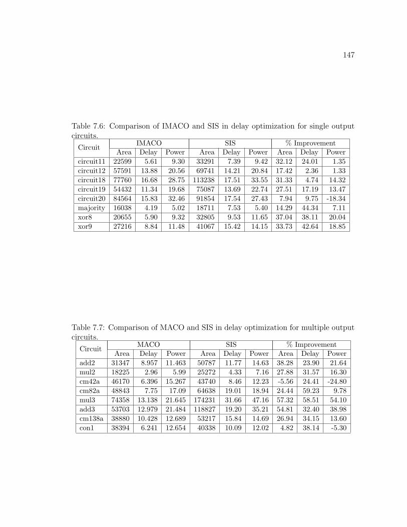
147
Table 7.6: Comparison of IMACO and SIS in delay optimization for single outputcircuits.
IMACO SIS % ImprovementCircuitArea Delay Power Area Delay Power Area Delay Power
circuit11 22599 5.61 9.30 33291 7.39 9.42 32.12 24.01 1.35circuit12 57591 13.88 20.56 69741 14.21 20.84 17.42 2.36 1.33circuit18 77760 16.68 28.75 113238 17.51 33.55 31.33 4.74 14.32circuit19 54432 11.34 19.68 75087 13.69 22.74 27.51 17.19 13.47circuit20 84564 15.83 32.46 91854 17.54 27.43 7.94 9.75 -18.34majority 16038 4.19 5.02 18711 7.53 5.40 14.29 44.34 7.11xor8 20655 5.90 9.32 32805 9.53 11.65 37.04 38.11 20.04xor9 27216 8.84 11.48 41067 15.42 14.15 33.73 42.64 18.85
Table 7.7: Comparison of MACO and SIS in delay optimization for multiple outputcircuits.
MACO SIS % ImprovementCircuitArea Delay Power Area Delay Power Area Delay Power
add2 31347 8.957 11.463 50787 11.77 14.63 38.28 23.90 21.64mul2 18225 2.96 5.99 25272 4.33 7.16 27.88 31.57 16.30cm42a 46170 6.396 15.267 43740 8.46 12.23 -5.56 24.41 -24.80cm82a 48843 7.75 17.09 64638 19.01 18.94 24.44 59.23 9.78mul3 74358 13.138 21.645 174231 31.66 47.16 57.32 58.51 54.10add3 53703 12.979 21.484 118827 19.20 35.21 54.81 32.40 38.98cm138a 38880 10.428 12.689 53217 15.84 14.69 26.94 34.15 13.60con1 38394 6.241 12.654 40338 10.09 12.02 4.82 38.14 -5.30

148
0.00
0.20
0.40
0.60
0.80
1.00
1.20
1.40
circuit11 circuit12 circuit18 circuit19 circuit20 majority xor8 xor9
Area Delay Power
Figure 7.6: Results of IMACO with DOAPC for single outputs functions, normalizedto SIS.
0.00
0.20
0.40
0.60
0.80
1.00
1.20
1.40
add2 mul2 cm42a cm82a mul3 add3 cm138a con1
Area Delay Power
Figure 7.7: Results of MACO with DOAPC for multiple outputs functions, normal-ized to SIS.

149
The tables show that the improvement in delay range from 2.36% (circuit12)
up to 59.23% (cm82a). In addition to that, significant area improvement of delay
optimized circuit is also observed. The graphical view of these results normalized
with respect to SIS is given in Figure 7.6 and Figure 7.7 for single output function
and multiple output functions, respectively.
As can be seen from the tables and figures above, in contrast with AODPC,
the results of DOAPC is very positive. The experiments show that the results
obtained from DOAPC is better compared to the ones obtained from SIS in all cases.
The reason behind this is the following. As mentioned in Chapter 2, ACO can be
easily modeled as a shortest path finding problem. Since delay can be considered
proportional to the length of the path, ACO algorithm, which is the basis for MACO,
provides a good computational tool for delay optimization problems.
7.3 Comparison with other Techniques
In this section, the proposed algorithm is compared to some other ELD techniques.
This includes a GA-based ELD and SimE-based ELD.
7.3.1 Comparison with GAs
The proposed algorithm is compared to the existing GA-based technique. Table 7.8
shows the comparison of MACO and GA [7]. The test case used is the first ten

150
randomly generated circuits. It should be noted that GA failed to deliver any
circuit bigger than those represented in the table.
The table shows that, except for circuit4, the proposed algorithm performs better
than GA in terms of area, delay and power. The highest improvement is obtained
in the case of circuit8, i.e., 90.29% area improvement, 78.41% delay improvement,
and 86.09% power improvement. Since circuit4 consists of one gate only, it can be
said that in general, MACO outperforms GAs.
Table 7.8: Comparison with GAs [7] technique in terms of area, delay and power.Coello [7] MACO % ImprovementCircuit
Area Delay Power Area Delay Power Area Delay Powercircuit1 18954 6.92 6.61 12879 5.57 4.97 32.05 19.57 24.77circuit2 21870 6.18 6.61 13122 5.18 5.28 40.00 16.13 20.06circuit3 19926 4.34 5.15 10692 3.05 3.82 46.34 29.84 25.86circuit4 1458 0.01 0.66 1458 0.01 0.67 0.00 0.00 0.00circuit5 27945 8.76 7.89 11664 5.57 5.08 58.26 36.46 35.67circuit6 40338 13.24 14.21 10935 3.34 3.82 72.89 74.77 73.13circuit7 83835 21.74 28.85 12393 5.59 4.37 85.22 74.28 84.85circuit8 75087 13.69 22.73 7290 2.96 3.16 90.29 78.41 86.09circuit9 104004 20.25 30.76 15066 5.42 5.27 85.51 73.23 82.85circuit10 97686 21.40 28.44 11178 5.42 4.06 88.56 74.67 85.72
Figure 7.8 shows the results of MACO algorithm for the given test cases. These
values are normalized with respect to the results obtained using GAs. It can be seen
that the area, delay and power of the solutions obtained by MACO are always ≤ 1.

151
0.0
0.2
0.4
0.6
0.8
1.0
1.2
circuit1 circui2 circuit3 circuit4 circuit5 circuit6 circuit7 circuit8 circuit9 circuit10
Area Delay Power
Figure 7.8: Comparison with GA: normalized area, delay and power are always ≤1.
Comparison in terms of execution time is given in Table 7.9. The percentage of
improvement is ≈ 99%. The table clearly shows that MACO algorithm is superior
as compared to GAs in terms of execution time. This result is not surprising since
GAs is a population-based heuristic. The time needed to find the solutions depends
not only on the number of iterations but also the size of the population used.
Table 7.9: Comparison with GA [7] technique in terms of execution time.Circuit Coello [7] MACO % Improvementcircuit1 8100 15.27 99.81circui2 12240 15.17 99.88circuit3 11052 14.67 99.87circuit4 11160 3.50 99.97circuit5 21132 16.97 99.92circuit6 30780 14.83 99.95circuit7 49068 16.10 99.97circuit8 57240 12.70 99.98circuit9 44784 83.21 99.81circuit10 61704 78.96 99.87

152
There exists other powerful iterative heuristics that have been used for solv-
ing optimization problem in VLSI design. One such heuristic is Simulated Evolu-
tion (SimE) [15]. Below, the proposed algorithm is compared to SimE-based ELD
technique [81].
7.3.2 Comparison with SimE
Table 7.10 and Table 7.11 show a comparison of the proposed algorithm with SimE-
based technique for area optimization and delay optimization, respectively.
Table 7.10: Comparison with SimE technique in terms of area, delay and power forarea optimization.
MACO SimE % ImprovementCircuitArea Delay Power Area Delay Power Area Delay Power
circuit1 12879 5.57 4.97 12879 3.90 4.97 0.00 -42.75 0.00circuit2 13122 5.18 5.28 13122 5.18 5.28 0.00 0.00 0.00circuit10 11178 5.42 4.06 9963 6.42 3.33 -12.20 15.58 -21.98circuit14 24786 7.25 9.20 23814 6.80 9.20 -4.08 -6.59 0.00circuit16 12393 5.71 4.26 9720 8.50 4.30 -27.50 32.78 0.88circuit17 10692 4.43 4.39 10692 4.43 4.39 0.00 0.00 0.00add2 24300 11.48 9.96 24300 11.48 9.96 0.00 0.00 0.00add3 49086 21.96 18.474 40265 26.73 14.83 -21.91 17.85 -24.57mul2 12636 3.56 4.66 12636 3.56 4.66 0.00 0.00 0.00mul3 59292 15.03 17.541 74358 13.14 21.65 20.26 -14.40 18.96cm42a 38880 7.45 13.25 38456 9.44 12.60 -1.10 21.08 -5.17cm82a 25272 10.45 9.96 25029 11.84 9.24 -0.97 11.78 -7.89b1 13851 1.53 5.91 11206 2.91 2.78 -23.60 47.46 -112.45con1 38151 6.698 13.741 30233 6.90 14.23 -26.19 2.93 3.44rd53 35235 15.32 14.00 38073 14.75 15.34 7.45 -3.88 8.75

153
Table 7.11: Comparison with SimE technique in terms of area, delay and power fordelay optimization.
MACO SimE % ImprovementCircuitArea Delay Power Area Delay Power Area Delay Power
circuit1 14823 3.86 6.41 15360 4.20 5.80 3.50 8.14 -10.47circuit2 17739 3.70 7.16 16870 3.88 6.90 -5.15 4.54 -3.70circuit10 12393 5.32 4.48 13771 5.50 4.77 10.01 3.22 6.02circuit14 30132 9.75 10.63 24786 7.25 9.20 -21.57 -34.52 -15.47circuit16 13122 5.71 4.26 10340 7.60 5.22 -26.91 24.82 18.35circuit17 12150 4.43 4.72 12354 5.30 5.38 1.65 16.47 12.23add2 31347 8.957 11.463 35270 9.37 12.66 11.12 4.41 9.45add3 53703 12.979 21.484 53703 12.98 21.48 0.00 0.00 0.00mul2 18225 2.96 5.99 18225 2.96 5.99 0.00 0.00 0.00mul3 74358 13.138 21.645 74358 13.14 21.65 0.00 0.00 0.00cm42a 91854 7.072 32.885 42768 5.19 15.02 -114.77 -36.37 -118.97cm82a 48843 7.75 17.09 55872 14.25 18.56 12.58 45.61 7.95b1 14580 1.49 6.24 12745 2.08 7.05 -14.40 28.61 11.49con1 38394 6.241 12.654 30233 6.90 14.23 -26.99 9.55 11.08rd53 53946 15.45 19.00 40201 13.10 15.98 -34.19 -17.90 -18.88
It can be seen in Table 7.10 that in eight out of fifteen cases, SimE produced
better circuits in terms of area. The worst solution produced by MACO is obtained
for circuit16, where the area improvement is -27.5%. There are only two cases in
which MACO produced circuits having better area, namely rd53 and mul3 circuits.
These results support our previous observation. The sharing of common sub-
functions that should be established by the sharing of pheromone trail, is not working
as expected. It is believed that there should be a new method to incorporate the
sharing of sub-functions in addition to the pheromone trails. It will be interesting
to further investigate this idea.
On the other hand, MACO algorithm provides some positive results in terms
of delay optimization. As shown in Table 7.11, in nine out of fifteen cases, MACO

154
provides better circuits in terms of delay. The highest improvement is obtained for
cm82a circuit. There are only three cases, in which SimE provides better results
in terms of delay. These results also support our previous observation in delay
optimization. Since ACO algorithm is basically a shortest path finding, MACO
works best for delay optimization.
7.4 Concluding Remarks
In this chapter, the results obtained using the introduced techniques were compared
with those obtained using the existing techniques. The proposed algorithms are
better in terms of design rate, quality of solution and execution time compared to
the existing ACO-based techniques. The proposed algorithms were also compared
to existing conventional tools, represented by SIS. It was observed that the area
optimization applied by the introduced algorithms performs better in most of the
cases, except for some multiple output circuits. However, the performance of delay
optimization of the proposed algorithms was better as compared to SIS.

Chapter 8
CONCLUSIONS AND FUTURE
DIRECTIONS
The dramatic increase in designer productivity over the past decade in the area of
VLSI (Very Large Scale Integration) circuit design can be attributed to the develop-
ment of sophisticated computer-aided design tools. The improvement in computer
aided design has been made possible by the advances in the field of logic synthesis.
In conventional logic design techniques, circuit designers begin with a precise
specification in the form of truth tables or Boolean expressions. These expressions
are manipulated by applying logic synthesis algorithms, such as factorization and
kernel extraction to minimize circuit representations. The outcome of logic synthesis
algorithms will be either in two-level, multi-level, or Reed Muller representations.
On the other hand, iterative heuristics work on larger space. Through the process
155

156
of assemble-and-test, candidate solutions are built and evaluated. At the end, the
optimum solution could evolve from this process.
This thesis offered a perspective for the automatic design of digital circuits
through evolutionary techniques. The use of assemble-and-test via iterative heuris-
tics has enabled the sampling of larger search space in circuit design problems. In
addition, modern issues in digital circuit design, such as low power and high perfor-
mance are addressed.
8.1 Conclusion
In this thesis, ACO-based evolutionary logic design techniques have been intro-
duced. The performance of the introduced algorithms have been compared to those
of existing conventional and evolutionary techniques.
Here are the concluding statements regarding the thesis work:
1. The introduced techniques successfully address the issue of circuits design,
considering modern design issues such as area, delay and power through the
use of iterative heuristics, multiobjective optimization and fuzzy logic.
2. It was observed that the introduced techniques have outperformed some of the
existing techniques in evolutionary logic design. The comparison is based on
the quality of solutions and time requirements.

157
3. Comparison with existing conventional techniques (represented by SIS) showed
that the introduced techniques produced better quality results in terms area,
delay and power for most of the test cases.
4. The improvement obtained using the introduced techniques in delay optimiza-
tion is better than area optimization.
8.2 Future Directions
Some possible directions for future work could be stated as follows:
1. Investigation of how to incorporate the sharing of sub-functions into the ACO
algorithm.
2. Investigation of the incorporation of some rules from logic synthesis domain
such as kernel extraction in order to improve the performance of the introduced
techniques.
3. Investigation of the use of some other iterative heuristics and possible hy-
bridization scheme can be performed in order to further improve the quality
of solutions.
Although the experiments have shown some good results, currently, the goal of
evolutionary logic design system is still far. The most stumbling block for evolu-
tionary techniques is the time taken to produce solutions. Approaches to improve

158
the execution time of current techniques such as parallelization are thus important
to explore. In addition, the advance of technology could allow us to use faster and
better machine as the platform for evolutionary logic design systems. Thus, the
dream of automated and efficient circuit design systems can be reached.

Appendix A
File Format and Circuit Used as
Test Cases
The following are the format of the required input files and the list of circuits used
as test cases during the experiments.
A.1 Library File Format
The gates’ parameters are obtained from CMOS MOSIS 0.25 m library. These
includes the following information:
1. The number of transistors (TRCOUNT)
2. The size of the gate (AREA)
3. The switching delay of the gate (BDELAY)
4. The input capacitance (CIN)
159

160
5. The output capacitance (COUT)
6. The load factor (LF)
Except for inverters and wires, there is more than one value for input capacitance.
In this regards, the higher value is considered. The same applied for the load factor.
The following shows the format of the library files used.
<GATE NAME> <TRCOUNT> <AREA> <BDELAY> <CIN> <COUT> <LF>
Using the above format, the library file considered in this thesis is given next.
WIRE 0 0 0 0 0 0
NOT 2 1215 3 2.661 0.005 516
AND 6 2187 9 2.661 0.005 553
OR 6 1944 11 2.661 0.004 567
XOR 10 3159 12 5.321 0.006 688
NAND 4 1458 5 2.661 0.007 444
NOR 4 1458 7 2.661 0.005 694
XNOR 10 2916 12 5.321 0.004 551
A.2 Input File Format
The proposed algorithms use PLA files as input. The parameters required by the
proposed algorithms are then generated automatically. However, if the circuits’
specification is not in the form of PLA files, the input file required by the algorithm
must contain the following information.

161
Field Description
maxrun The number of maximum runs to be performed by the algorithm
maxiter The number of maximum iterations for a single run
objtype The optimization objective of the current action.
(0 = gatecount, 1 = area, 2 = delay, and 3 = power)
ifdweight Static (0) or dynamic (1) weight is employed
weight The value Wf at the beginning of the iteration
ifphase Positive (0) or negative (1) phase is used.
In positive mode, all literals are uncomplemented. In negative mode,
some literals can be in the complemented forms, depending on its
functional fitness. (not used, default = 0)
dataset The number of input dataset. Useful for generating truth table for
arithmetic circuits such as adders, multipliers. For example, a 2-bit
adder has dataset value equal to 2. (not used, default value = 1)
numvar Number of inputs
numout Number of outputs
invin Set to ‘1’ if complemented literals are used in addition
to uncomplemented ones. (default = 0)
row The number of rows at the beginning of the iteration
level The number of columns at the beginning of the iteration
iflocal Set to 1 if local search is employed (not used)
gatemode The type of library used. Values are within [0-7]
gcmax Set the maximum number of gates allowed for a circuit (not used)
gcmin Set the minimum number of gates allowed for a circuit (not used)
numant Set the number of ants used

162
Field Description
maxgen Set the maximum number of generations of ant
gamma Set the constant for pheromone update calculation
rho Set the pheromone evaporation rate
range tau Set the maximum range of pheromone values allowed
ttf[0] The string of truth table of the first output of the circuit
ttf[1] The string of truth table of the second output of the circuit (if available)
ttf[k] The string of truth table of the k+1 output of the circuit (if available)
A.3 Randomly Generated Circuits
There are 20 randomly generated circuits used in the experiments. These circuits are
listed below.
circuit input(s) output(s) circuit input(s) output(s)circuit1.pla 4 1 circuit11.pla 5 1circuit2.pla 4 1 circuit12.pla 6 1circuit3.pla 4 1 circuit13.pla 5 1circuit4.pla 2 1 circuit14.pla 6 1circuit5.pla 4 1 circuit15.pla 6 1circuit6.pla 4 1 circuit16.pla 6 1circuit7.pla 4 1 circuit17.pla 5 1circuit8.pla 4 1 circuit18.pla 6 1circuit9.pla 6 1 circuit19.pla 6 1circuit10.pla 6 1 circuit20.pla 6 1
A.4 Benchmark Circuits
There are 14 benchmark circuits used in the experiments. These circuits are listed below.

163
circuit input output circuit input output
majority.pla 5 1 b1.pla 3 4
xor8.pla 8 1 C17.pla 5 2
xor9.pla 9 1 cm138a.pla 6 8
add2.pla 5 3 cm42a.pla 4 10
add3.pla 7 4 cm82a.pla 5 3
mul2.pla 4 4 con1.pla 7 2
mul3.pla 6 6 rd53.pla 5 3

Bibliography
[1] J. F. Miller, D. Job, and Vassilev V. K. Principles in the Evolutionary Design
of Digital Circuits - Part I. Journal of Genetic Programming and Evolvable
Machines, 1(1):8–35, 2000.
[2] J. F. Miller, T. Fogarty, and P Thomson. Designing Electronic Circuits Using
Evolutionary Algorithms. Arithmetic Circuits: A Case Study. Genetic Al-
gorithms and Evolution Strategy in Engineering and Computer Science, John
Wiley and Sons, Chichester, pages 105–131, 1998.
[3] J. F. Miller and P. Thomson. Aspects of Digital Evolution: Geometry and
Learning. Proceedings of Second International Conference on Evolvable Systems
(ICES’98) Lecture Notes in Computer Science, 1478:25–35, Springer-Verlag,
Heidelburg, 1998.
[4] J. F. Miller and P. Thomson. Discovering Novel Digital Circuits Using Evo-
lutionary Techniques. IEE Colloquium on Evolvable Systems, Savoy Place,
London, March 1998.
164

165
[5] J. F. Miller and P. Thomson. Aspects of Digital Evolution: Evolvability and
Architecture. Proceedings of Fifth International Conference on Parallel Problem
Solving From Nature (PPSN’98) Lecture Notes in Computer Science, 1498:927–
936, Springer-Verlag, Heidelburg, 1998.
[6] C. A. Coello, A. D. Christiansen, and A. H. Aguirre. Ant Colony System for
the Design of Combinational Logic Circuits. Evolvable Systems: From Biology
to Hardware, Edinburgh, Scotland, pages 21–30, April Springer Verlag, 2000.
[7] C. A. Coello, A. D. Christiansen, and A. H. Aguirre. Use of Evolutionary
Techniques to Automate the Design of Combinational Circuits. International
Journal of Smart Engineering System Design, Elsevier Science, 2(4):299–314,
June 2000.
[8] Giovanni De Micheli. Synthesis and Optimization of Digital Circuits. McGraw-
Hill, New York, 1994.
[9] M. Dorigo, Gianni Di Caro, and Luca M. Gambardella. Ant Algorithms for
Discrete Optimization. Technical Report Tech. Rep. IRIDIA/98-10, IRIDIA,
Universite Libre de Bruxelles, Brussels, Belgium, 1998.
[10] Sushil J. Louis. Genetic Algorithms as a Computational Tool for Design. PhD
thesis, Department of Computer Science, Indiana University, Aug 1993.

166
[11] C. A. Coello, A. D. Christiansen, and A. H. Aguirre. Towards Automated
Evolutionary Design of Combinational Circuits. Computers and Electrical En-
gineering, Pergamon Press, 27(1):1–28, Jan. 2001.
[12] B. Hounsell and T. Arslan. A Novel Genetic Algorithm for the Automated
Design of Performance Driven Digital Circuits. CEC-2000, pages 601–608,
2000.
[13] B. Hounsell and T. Arslan. A Novel Evolvable Hardware Framework for the
Evolution of High Performance Digital Circuits. GECCO-2000, pages 525 –
532, July 2000.
[14] M. Dorigo and M. Maniezzo and A. Colorni. The Ant Systems: An Autocat-
alytic Optimizing Process. Revised 91-016, Dept. of Electronica, Milan Poly-
technic, 1991.
[15] Sadiq M. Sait and H. Youssef. Iterative Computer Algorithms with Applica-
tions in Engineering: Solving Combinatorial Optimization Problems. IEEE
Computer Society Press, 1999.
[16] W. Quine. The Problem of Simplifying Truth Functions. American Mathemat-
ical Monthly, 59:521–531, 1952.
[17] E. McCluskey. Minimisation of Boolean Function. Bell System Technical Jour-
nal, 38:1417–1444, 1956.

167
[18] R. Brayton, G. D. Hachtel, C. T. McMullen, and A.L. Sangiovanni-Vincentelli.
Logic Minimisation Algorithms for VLSI Synthesis. Kluwer Academic Pub-
lisher, 1984.
[19] R. Brayton, R. Rudell, A. L. Sangiovanni-Vincentelli, and A. Wang. MIS: A
Muliple-Level Logic Optimisation System. IEEE Trans. on Computer-Aided
Design, CAD-6:1062–1081, Nov. 1987.
[20] R. Brayton, G. D. Hachtel, and A. L. Sangiovanni-Vincentelli. Multilevel Logic
Synthesis. Proceeding of the IEEE, 78:264–300, Feb. 1990.
[21] E. M. Sentovic, K. J. Singh, L. Lavagno, C. Moon, R. Murgai, A. Saldanha,
H. Savoj, P. R. Stephan, R. K. Brayton, and A. L. Sangiovanni-Vincentelli.
SIS: A System for Sequential Circuit Synthesis. Technical Report UCB/ERL
M92/41, University of California, Berkeley, May 1992.
[22] D. Bostick et al. The Boulder Optimal Logic Design System. Proceeding of the
International Conference on CAD, pages 62–65, Nov. 1987.
[23] Hugo de Garis. Evolvable Hardware: Genetic Programming of a Darwin Ma-
chine. Proceedings of the International Conference in Innsbruck, Austria, pages
441–449, Springer-Verlag, 1993.
[24] R. S. Zebulum, M. A. Pacheco, and Marley Vellasco. Evolvable Systems in
Hardware Design: Taxonomy, Survey and Applications. Evolvable System:
168
From Biology to Hardware. Proceeding of the First International Conference,
ICES 96 Tsukba, Japan, Lecture Notes in Computer Science, 1259:344–358,
Oct. 1997.
[25] R. S. Zebulum and M. A. Pacheco and Maria Vellasco. Evolutionary Electronics:
Automatic Design of Electronic Circuits and Systems by Genetic Algorithms.
CRC Press, 2002.
[26] T. Higuchi, T. Niwa, T. Tanaka, H. Iba, H. de Garis, and T. Furuya. Evolving
Hardware with Genetic Learning: A First Step Towards Building a Darwin
Machine. Proceeding of the 2nd Int. Conf. on The Simulation of Adaptive
Behavior (SAB92), pages 417–427, MIT Press, Aug. 1993.
[27] J. R. Koza. Genetic Programming: On the Programming of Computers by
Means of Natural Selection. MIT Press, 1992.
[28] Adrian Thompson. Silicon Evolution. Proceedings of the First Annual Confer-
ence on Genetic Programming, pages 444–452, MIT Press, 1996.
[29] J. R. Koza, F. H. Bennett, D. Andre, and M. A. Keane. Automated Design
of Both the Topology and Sizing of Analogue Electrical Circuits Using Genetic
Programming. Artificial Intelligent in Design, pages 151–170, Kluwer Academic
Publishers, 1996.

169
[30] J. R. Koza, F. H. Bennett, D. Andre, and M. A. Keane. Genetic Program-
ming III: Darwinian Invention and Problem Solving. Morgan Kaufmann, San
Fransisco, CA, 1999.
[31] T. Higuchi, M. Iwata, I. Kajitani, M. Murakawa, S. Yoshizawa, and T. Furuya.
Hardware Evolution at Gate and Functional Level. Proceeding of the Interna-
tional Conference on Biologically Inspired Autonomous Systems: Computation,
Cognition and Action, March Durham, USA, 1996.
[32] Moshe Sipper et. al. A Phylogenetic, Ontogenetic, and Epigenetic View of
Bio-Inspired Hardware Systems. IEEE Trans. on Evolutionary Computation,
1(1):83–97, 1997.
[33] Xin Yao and Tetsuya Higuchi. Promises and Challenges of Evolvable Hardware.
IEEE Trans. on Systems, Man, and Cybernetics - Part C: Applications and
Reviews, 29(1):87–97, 1999.
[34] J. F. Miller and P. Thomson. A Developmental Method for Growing Graphs and
Circuits. Fifth International Conference on Evolvable Systems: From Biology
to Hardware, 2606:93–104, Mar 2003.
[35] T. Fogarty, J. F. Miller, and P. Thomson. Evolving Digital Logic Circuits on
Xilinx 6000 Family FPGAs. The 2nd Online Conference on Soft Computing in

170
Engineering Design and Manufacturing, pages 299–305, Springer-Verlag, Lon-
don, 1998.
[36] C. A. Coello and Hernndez Aguirre, Arturo,. Evolutionary Multiobjective De-
sign of Combinational Logic Circuits. Proceedings of the Second NASA/DoD
Workshop on Evolvable Hardware, pages 161–170, Jul 2000.
[37] C. A. Coello, and Hernandez Luna, Erika and Hernandez Aguirre, Arturo,.
Use of Particle Swarm Optimization to Design Combinational Logic Circuits.
Evolvable Systems: From Biology to Hardware. 5th International Conference,
ICES 2003, 2606:398–409, Mar 2003.
[38] C. Y. Lee. Representation of Switching Circuit by Binary Decision Programs.
Bell Systems Technical Journal, 38:985–999, 1959.
[39] S. J. Hong, R. G. Cain, and D. L. Ostapko. MINI: A Heuristic Approach for
Logic Minimization. IBM Journal of Research and Development, 18:443–458,
Sept. 1974.
[40] L. Berman and L. Trevillyan. A Global Approach to Circuit Size Reduction.
Advance Research in VLSI, 5th MIT Conference, pages 203 – 214, 1988.
[41] Shih-Chieh Chang and malgorzata Marek-Sadowska and Kwang-Ting Cheng.
Perturb and Simplify: Multilevel Boolean Network Optimizer. IEEE Trans.
171
Computer Aided Design of Integrated Circuits and Systems, 15(12):1494 – 1504,
Dec 1996.
[42] Shih-Chieh Chang and David Ihsin Cheng. Efficient Boolean Division and Sub-
stitution Using Redundancy Addition and Removing. IEEE Trans. Computer
Aided Design of Integrated Circuits and Systems, 18(8):1096 – 1106, Aug 1999.
[43] S. Muroga and Y. Kambayashi and H. C. Lai and J.N. Culliney. The Trans-
duction Method – Design of Logic Networks Based on Permissible Functions.
IEEE Trans. Computer, 38(10):1404–1424, 1989.
[44] S. B. Akers. Binary decision diagrams. IEEE Trans. on Computers, 27:509–516,
1978.
[45] R. Bryant. Graph-based Algorithms for Boolean Function Manipulation. IEEE
Trans. on Computers, 35:677–691, 1986.
[46] Soha Hassoun and Tsutomu Sasao. Logic Synthesis and Verification. Kluwer
Academic Publisher, Massachusetts, USA, 2002.
[47] D. Green. Modern Logic Design. Addison-Wesley, Reading, MA, 1986.
[48] T. Sasao. Logic Synthesis and Optimisation. Kluwer Academic Publisher, 1993.
172
[49] Deo Singh, J.M. Rabaey, Massoud Pedram, Francky Catthoor, Suresh Raj-
gopal, Naresh Sehgal, and T.J. Mozdzen. Power Conscious CAD Tools and
Methodologies: A Perspective. IEEE Proceeding, 83(4):570 – 594, April 1995.
[50] Massoud Pedram. Power Minimization in IC Design: Principles and Applica-
tions. ACM Trans. Design Automation of Electronic Systems, 1(1):3 – 56, Jan.
1996.
[51] Massoud Pedram. Logical-Physical Co-design for Deep Submicron Circuits:
Challenges and Solutions. Proceedings of Design Automation Conference, the
ASP-DAC’98. Asia and South Pacific,, pages 137 – 142, Feb. 1998.
[52] Sasan Iman and Massoud Pedram. POSE: Power Optimization and Synthesis
Environment. ACM 33rd Design Automation Conference, DAC’96, pages 21 –
26, Jan. 1996.
[53] S. Goss, S. Aron, J. L. Deneubourg, and J. M. Pasteels. Self-organized Shorcuts
in the Argentine Ant. Naturwissenschaften, 76:579–581, 1989.
[54] M. Dorigo and G. Di Caro. New Ideas in Optimisation. McGraw Hill, London,
UK, 1999.
[55] M. Dorigo and T. Stutzle. The ant colony optimization metaheuristic: Algo-
rithms, applications, and advances, 2002.

173
[56] Carlos M. Fonseca and Peter J. Fleming. Multiobjective Optimization and
Multiple Constraint Handling with Evolutionary Algorithms I: A Unified For-
mulation. Technical report, Dept. of Automatic Control and System Eng.,
University of Sheffield, Sheffield, U.K., Jan. 1995.
[57] L.A. Zadeh. Fuzzy sets. Information and Control, 8(3):338–353, June 1965.
[58] L. A. Zadeh. Outline of a new approach to the analysis of complex systems and
decision processes. IEEE Transaction Systems Man. Cybern, SMC-3(1):28–44,
1973.
[59] J. M. Mendel. Fuzzy logic systems for engineering: A tutorial. IEEE Proceeding,
83(3):345–377, Mar. 1995.
[60] E. Q. Kang, Rung-Bin Lin, and E. Shragowitz. Fuzzy logic approach to vlsi
placement. IEEE Trans. on Very Large Scale Integration (VLSI) Systems,
2(4):489–501, Dec. 1994.
[61] E. Shragowitz, Jun-Yong Lee, and E. Q. Kang. Application of fuzzy logic in
computer aided design. IEEE Trans. on Fuzzy Systems, 6(1):163–172, Feb.
1998.
[62] Sadiq M. Sait and Youssef, H. and J. A. Khan and El-Maleh, A. Fuzzy sim-
ulated evolution for power and performance optimization of VLSI placement.

174
Proceedings of International Joint Conference on Neural Networks, IJCNN ’01.,
1:738 –743, July 2001.
[63] H. J. Zimmerman. Fuzzy Set Theory and Its Applications. Kluwer Academic
Publishers, 3rd edition, 1996.
[64] L. A. Zadeh. The concept of linguistic variable and its application to approxi-
mate reasoning. Information Science, 8:199–249, 1975.
[65] Ronald R. Yager. On Ordered Weighted Averaging Aggregation Operators
in Multicriteria Decision Making. IEEE Transaction on Systems, MAN, and
Cybernetics, 18(1):183–190, Jan 1988.
[66] R. Yager. Multiple objective decision-making using fuzzy sets. International
Journal of Man-Machine Studies, pages 9:375–382, 1977.
[67] R. Yager. Second Order Structures in multi-criteria decision making. Interna-
tional Journal of Man-Machine Studies, pages 36:553–570, 1992.
[68] Hernndez Aguirre, Arturo, and Buckles, Bill P. and C. A. Coello. Gate-level
Synthesis of Boolean Functions using Binary Multiplexers and Genetic Pro-
gramming. Congress on Evolutionary Computation,, pages 675–682, Jul 2000.
[69] J. F. Miller and P. Thomson. Cartesian genetic programming. Third European
Conference on Genetic Programming Edinburgh, 1802:121–132, Apr 2000.

175
[70] D. Montana and R. Popp, and G. Vidaver and S. Iyer. EvolWare: Genetic
Programming for Optimal Design of Hardware Based Algorithm. Third Annual
Conference on Genetic Programming, pages 869–874, July 1998.
[71] J. M. Sanchez and J. Lanchares. Multilevel Logic Synthesis Using Algorithm
Based on Natural Processes. Proceeding of the 20th International Conference
on Microelectronics, 2:823–828, Sep 1995.
[72] J. Miller and P Thomson. Combinational and Sequential Logic Optimisation
using Genetic Algorithms. GALESIA: 1st IEEE/IEE Joint International Con-
ference on GA Applications, pages 34–38, Sep 1995.
[73] J. Miller and P. Thomson. Restricted Evaluation Genetic Algorithms with Tabu
Search for Optimising Boolean Functions as Multi-level AND-EXOR Networks.
AISB Workshop on Genetic Algorithms and Evolutionary Techniques, 1143:85–
101, Apr 1996.
[74] Rolf Dreschsler. Evolutionary Algorithms for VLSI CAD. Kluwer Academic
Publisher, Boston, 1998.
[75] Sasan Iman and Massoud Pedram. Two-level Logic Minimization for Low
Power. IEEE/ACM International Conference on Computer-Aided Design,
ICCAD-95, pages 433 – 438, Nov 1995.
176
[76] Sasan Iman and Massoud Pedram. An Approach for Multilevel Logic OPtimiza-
tion Targetting Low Power. IEEE Trans. Computer Aided Design of Integrated
Circuits and Systems, 15(8):889 – 901, Aug. 1996.
[77] Priya Patil, Tan-Li Chou, Kaushik Roy, and Rabindra Roy. Low-Power Driven
Logic Synthesis Using Accurate Power Estimation Techniques. 10th Interna-
tional Conference on VLSI Design, pages 179 – 184, Jan. 1997.
[78] Chih-Shun Ding, Chi-Ying Tsui, and Masoud Pedram. Gate Level Power Esti-
mation Using Tagged Probabilistic Simulation. IEEE Trans. Computer Aided
of Integrated Circuit and Systems, 17(11):1099 – 1107, Nov. 1998.
[79] Srinivas Devadas and Sharad Malik. A Survey of Optimization Techniques
Targeting Low Power VLSI Circuits. 32nd ACM/IEEE Design Automation
Conference, pages 242–247, 1995.
[80] Standard Cell Library for MOSIS CMOS,
http://www.mosis.org/Technical/Designsupport/std-cell-library-scmos.html.
[81] Uthman Al-Saiari. Combinational logic circuits design through simulated evo-
lution. Master’s thesis, King Fahd University of Petroleum and Minerals,
Dhahran, KSA, November 2003.

VITA
• Bambang Ali Basyah Sarif
• Born in Jakarta, Indonesia, 14 March 1977.
• Received Bachelor Degree in Electrical Engineering from
Bandung Institute of Technology, Bandung, Indonesia in February 2000.
• Joined Computer Engineering Department, KFUPM, as a
Research Assistant in January 2001.
• Received Master of Science Degree in Computer Engineering from
KFUPM, Dhahran, Saudi Arabia in November 2003.
Related Documents