Development of a Graphic User Interface for an Overhead ... Executive Summary This project developed a graphic user interface (GUI) and estimation software package for the depiction

Development of a Graphic User Interfacefor an Overhead Conductor Sag Instrument

Final Project Report

Power Systems Engineering Research Center

A National Science FoundationIndustry/University Cooperative Research Center

since 1996

PSERC

Power Systems Engineering Research Center

The Development of a Graphic User Interface for an Overhead Conductor Sag Instrument

Sag Monitoring for Overhead Transmission Lines

Final Report

G. T. Heydt, Project Leader Arizona State University

PSERC Publication 02-24

April 2002

Information about this Project For information about this project contact: G. T. Heydt Regents’ Professor Arizona State University Department of Electrical Engineering PO Box 875706 Tempe, AZ 85287-5706 Phone: 480 965 8307 Fax: 480 965 0745 Email: [email protected] Power Systems Engineering Research Center This is a project report from the Power Systems Engineering Research Center (PSERC). PSERC is a multi-university Center conducting research on challenges facing a restructuring electric power industry and educating the next generation of power engineers. More information about PSERC can be found at the Center’s website: http://www.pserc.wisc.edu. For additional information, contact: Power Systems Engineering Research Center Cornell University 428 Phillips Hall Ithaca, New York 14853 Phone: 607-255-5601 Fax: 607-255-8871 Notice Concerning Copyright Material Permission to copy without fee all or part of this publication is granted if appropriate attribution is given to this document as the source material. This report is available for downloading from the PSERC website.

2002 Arizona State University. All rights reserved.

Acknowledgements The work described in this report was sponsored by the Power Systems Engineering

Research Center (PSERC). We express our appreciation for the support provided by

PSERC’s industrial members and by the National Science Foundation under grant NSF

EEC 0001880 received under the Industry/University Cooperative Research Center

program.

Our thanks is given to Entergy for its support of this project and the prior project leading

to this work. Thanks is also given to the following individuals who contributed to this

project:

Baj Agrawal Arizona Public Service Company Industry advisor

Floyd Galvan Entergy Industry advisor

Robert G. Olsen Washington State University University advisor

Lance Priez Entergy Industry advisor

John Schilleci Entergy Industry advisor

ii

Executive Summary

This project developed a graphic user interface (GUI) and estimation software package

for the depiction of transmission line sag data and the calculation of real time conductor

rating. A GUI was developed in Visual Basic 6.0. The GUI appears to give the kind of

information that an operator may desire in a graphical sense. The software can be

connected to any suitable database written as a text file or as a standard database (such as

Microsoft Access). The software is available as an engineering prototype. This report

contains the main results of the development of the GUI. A sample listing of the main

frame code is given. A summary of previous work on the development of a sag

instrument based on Global Positioning Satellite technology is also given.

iii

Table of Contents Section Page1 Introduction and motivation 1 2 Statement of the research work 2 3 Relationship to a previous project: “The use of the Global Positioning

System (GPS) to measure the sag of overhead conductors” 2

4 Theoretical basis for signal processing overhead sag data 4 5 The least squares formula 4 6 Performance of the estimator as a real time circuit rating calculator 5 7 Conclusions and recommendations 6 Appendix A: A Sampling of the Visual Basic 6.0 Main Engine 7 A.1 Capabilities of Visual Basic 6.0 7 A.2 An Example of the Code Used to Generate the Visual Basic GUI for Sag

Monitoring / Processing (Program GRANDLINE) 8

Appendix B: Report of Main Results from the GPS Instrument Development 11 B.1 Citation 11 B.2 Abstract of main results 11 B.3 Overhead conductor ratings 11 B.4 The Global Positioning System 12 B.5 GPS measurement of overhead conductor sag 14 B.6 Data processing from the GPS 15 B.7 Power supply and communications link 19 B.8 Signal processing results 21 B.9 Conclusions 23 References 23

The Development of a Graphic User Interface for an Overhead Conductor Sag Instrument

1 Introduction and motivation

The main motivation of this work is in the measurement of the physical sag of overheated transmission conductors for the purpose of increasing line loading. The electrical load of conductors causes I2R heat to be dissipated in the conductor, and ambient environmental conditions and conductor tension determine the sag. If the sag is allowed to be too great, the conductor could be damaged. Therefore, line ratings are traditionally set conservatively as static values. When ambient conditions permit, it may be possible to load the conductor to higher levels, and therefore transmission capacity may be increased. In a modern deregulated environment, the additional transmission capacity may be used or sold. The increase in line loading is therefore related to financial benefit. The present project builds on an earlier project at Arizona State University. The main objective of the present project is to utilize the latest methods of digital signal processing to obtain accurate sag from physical measurements. The measurements may be from several types of instruments. The processing should be done to give an estimate of the present line loading capability. This should be done in a user friendly interface, namely a graphic user interface of object oriented menu. 2 Statement of the research work

The project scope is for the development of a real time transmission line rating calculator utilizing both standard transmission circuit ratings as well as real time sag measurement. This is a software development that is proposed to the demonstration stage. There are three key elements of the project.

• The development of a graphic user interface that allows the calculation of real time transmission line rating.

• The basis of the software will be Visual C++.

• Real time dynamic line data (including sag) from any source will be inputs.

3 Relationship to a previous project: The use of the Global Positioning System

(GPS) to measure the sag of overhead conductors

In 2000, Entergy funded a pilot project for the development of an instrument that uses the GPS to measure sag. The basic concept is depicted in Figure (1). That project resulted in the design of a prototype instrument that was tested at low transmission line power. The device uses a low power differential GPS receiver plus a spread spectrum

2

transceiver to form a differential GPS instrument. One of the two GPS receives in the differential configuration is located on the transmission line. The altitude reading of the remote GPS is reported to a base station receiver where digital signal processing and correction is done. In a laboratory environment, the instrument produces 17 cm error or less 70% of the time. Figure (2) shows the distribution of error in GPS instrumentation in this application. The cost of the unit is mainly the packaging cost of the GPS instrument on the transmission line. The differential GPS receivers are relatively low cost. The project ended in 2000. Appendix B references relevant publications and contains the main results of this previous project.

ROVER

SATELLITE

SAG

BASE

PSEUDORANDOMCODE

Figure (1) Basic concept of a GPS instrument to measure the sag of an overhead conductor

3

Cum

ulat

ive

distr

ibut

ion

(%)

B ad data rejec ted (— )R aw data (- - -)

A bsolu te va lue of error (m )

Figure (2) The cumulative distribution of error in a differential GPS instrument to measure overhead conductor sag

4 Theoretical basis for signal processing overhead sag data

The concept is to utilize data from a sag measurement instrument to determine the real time rating of an overhead transmission conductor. The general configuration is illustrated in Figure (3).

Sagmeasurement

instrument

Time stampedhistoricalweather data,circuit loading

Use of a leastsquares

formula forsag as a

function ofknown

parametersand unknowncoefficients

Using maximum sag =coefficients * (knowncircuit load, unknownmax current), solve formaximum conductorcurrent to give max sag

REA

L TI

ME

CIR

CU

ITR

ATIN

G

Figure (3) Use of sag measurements to determine the real time rating of an overhead transmission conductor

4

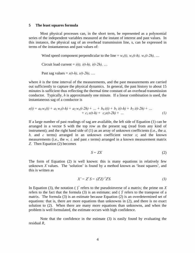
5 The least squares formula

Most physical processes can, in the short term, be represented as a polynomial series of the independent variables measured at the instant of interest and past values. In this instance, the physical sag of an overhead transmission line, s, can be expressed in terms of the instantaneous and past values of:

Wind speed component perpendicular to the line = ws(t), ws(t-h), ws(t-2h), … Circuit load current = i(t), i(t-h), i(t-2h), … Past sag values = s(t-h), s(t-2h), …

where h is the time interval of the measurements, and the past measurements are carried out sufficiently to capture the physical dynamics. In general, the past history to about 15 minutes is sufficient thus reflecting the thermal time constant of an overhead transmission conductor. Typically, h is approximately one minute. If a linear combination is used, the instantaneous sag of a conductor is s(t) = a0 ws(t) + a1 ws(t-h) + a2 ws(t-2h) + … + b0 i(t) + b1 i(t-h) + b2 i(t-2h) + …

+ c1 s(t-h) + c2s(t-2h) + … (1) If a large number of past readings of sag are available, the left side of Equation (1) can be arranged in a vector S with the top row as the present sag (read from any kind of instrument); and the right hand side of (1) as an array of unknown coefficients (i.e., the a, b, and c terms) arranged in an unknown coefficient vector x; and the known measurements (i.e., the w, i, and past s terms) arranged in a known measurement matrix Z. Then Equation (2) becomes

S = ZX (2) The form of Equation (2) is well known: this is many equations in relatively few unknown X values. The ‘solution’ is found by a method known as ‘least squares’, and this is written as

X’ = Z+S = (ZtZ)-1ZtS. (3) In Equation (3), the notation ( )+ refers to the pseudoinverse of a matrix; the prime on X refers to the fact that the formula (3) is an estimate; and ( )t refers to the transpose of a matrix. The formula (3) is an estimate because Equation (2) is an overdetermined set of equations: that is, there are more equations than unknowns in (2), and there is no exact solution to (2). When there are many more equations than unknowns, and when the problem is well formulated, the estimate occurs with high confidence. Note that the confidence in the estimate (3) is easily found by evaluating the residual R,

5

R = | ZX’ – S |, That is the residual R is simply the norm of the difference of the right and left hand side of Equation (2). R is a measure of how well X’ fits the equations. If R is large, the error is large, and there is low confidence in the solution. In a typical formulation, the dimensions of the matrices and vectors are: measurements Z is about 44 by 50 (i.e., 15 wind speeds, 15 currents, and 14 sags over 50 past readings); X is about 44; and S (past sags) is about 50. The residual R is a scalar. 6 Performance of the estimator as a real time circuit rating calculator

The expression (3) and the residual formula have been programmed in Visual Basic 6.0. The concept is illustrated in Figure (1). The pseudoinverse is carried out using the Shipley Coleman method for matrix inversion. The software was attached to synthetic data generated only for this prototype. The result is illustrated in Figure (4). The calculation is done virtually instantaneously in the prototype. The confidence is depicted in section 4 of the graphic user interface as a colored circle: green for high confidence, yellow for caution, and red for low confidence. In theory, this GUI can get attached to data from any sag instrument. The only requirement is that the software must be able to read the data format.

Figure (4) A graphic user interface for the calculation of a real time rating of an overhead transmission circuit based on sag

6

7 Conclusions and recommendations

The main conclusion of this project is that it is possible to develop a single form transmission line rating GUI. The GUI will calculate real time overhead transmission conductor ratings. The inputs are sag, line load current, and wind speed / direction. The validity of the GUI has been demonstrated in laboratory conditions. The basis of the GUI is an estimation technique that uses the least squares method. The recommendations are that the GUI should be improved as follows:

• To show the real time line load and sag

• To improve the confidence indicator

• To test the GUI in actual line conditions

• To couple the GUI to an operative sag instrument.

7

Appendix A

A Sampling of the Visual Basic 6.0 Main Engine A.1 Capabilities of Visual Basic 6.0 Visual Basic 6.0 is a graphic computer language that is used to develop object oriented programs. These are programs that are popularly known as menu driven programs, and they involve menus, pull-down tabs, command buttons, and many other graphic devices that appear on the CRT screen. Examples are Microsoft Word and Microsoft PowerPoint. The language is similar to Visual C++, Visual J++, and some other graphic languages.

A Visual Basic 6.0 program is made up of code, and the code is broken into procedures, assignments, commands, and lower syntax forms. The main elements are procedures that are basically subroutines.

Although Visual Basic 6.0 is an outgrowth of Basic, Visual Basic 6.0 differs

dramatically from the Basic language of 20 years ago. Visual Basic 6.0 is a sophisticated language that is powerful, is highly integrated with C, C++, Visual C++, and Java related languages. That is, it is easy to import subroutines from these languages to Visual Basic 6.0. In fact, the syntax of Visual Basic 6.0 and the other cited languages is rather similar. In addition to the integration of these languages, Visual Basic 6.0 can access a range of Microsoft products such as Excel and Access. That is, data in many other Microsoft products can be imported into Visual Basic 6.0 with a single simple syntax statement.

A main advantage of Visual Basic 6.0 is the ease in which complex forms (i.e.,

menus) can be generated. Professional forms are possible by a drag-and-click technique: programming is mainly using a selection procedure that involves drag-and-click operations. It is also possible to program in the usual way by entering syntax line by line. Perhaps the main disadvantages of Visual Basic 6.0 are the long length of typical programs, relatively inconvenient procedures needed to run compiled programs on computers that do not have Visual Basic 6.0 installed, and the fairly strong commitment to Microsoft Access as a database language. All these problems are relatively minor, and no true special skills are needed to obtain very good results. It is conjectured, however, that a dedicated professional programmer would be needed to develop production grade Visual Basic 6.0 software. The subsequent section contains a small sample of code in Visual Basic 6.0. The sample is part of the code used to generate the forms used in the body of this report.

8

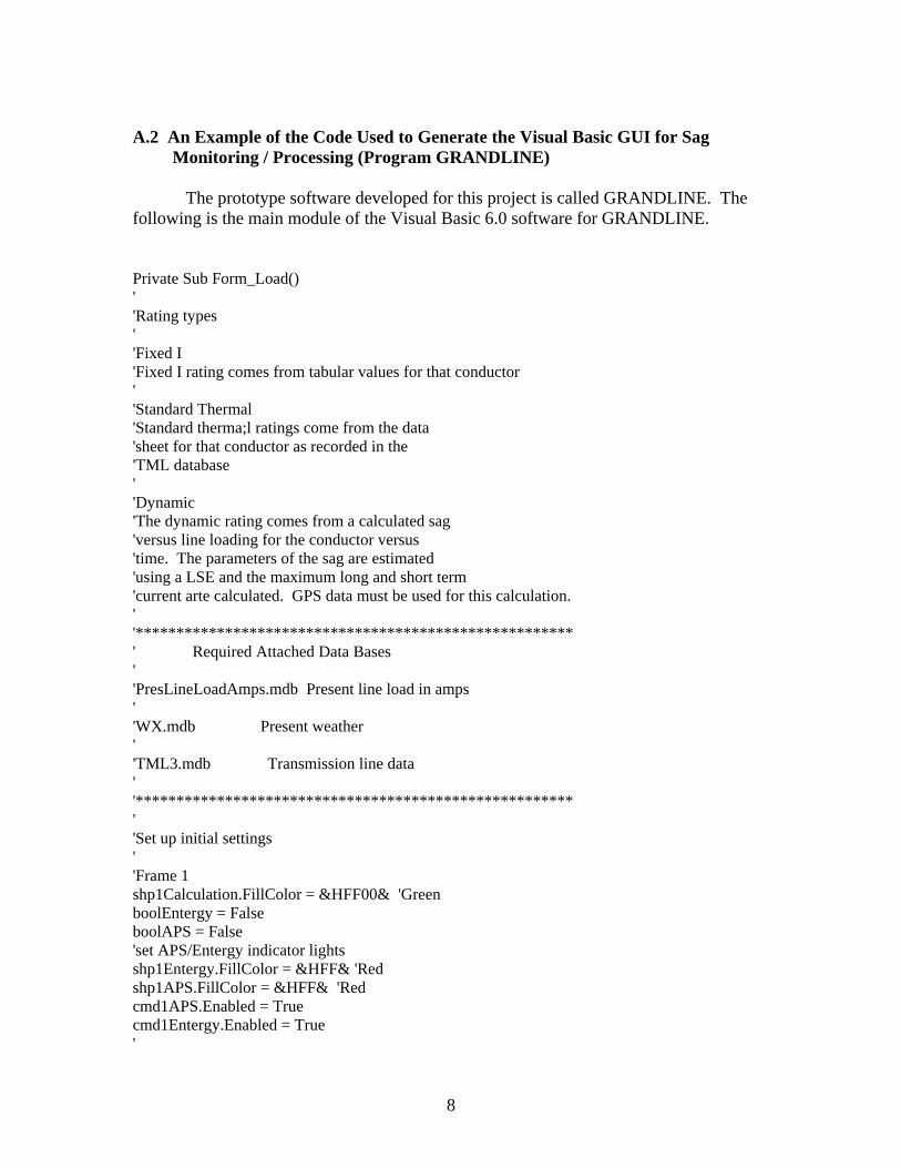
A.2 An Example of the Code Used to Generate the Visual Basic GUI for Sag

Monitoring / Processing (Program GRANDLINE) The prototype software developed for this project is called GRANDLINE. The following is the main module of the Visual Basic 6.0 software for GRANDLINE. Private Sub Form_Load() ' 'Rating types ' 'Fixed I 'Fixed I rating comes from tabular values for that conductor ' 'Standard Thermal 'Standard therma;l ratings come from the data 'sheet for that conductor as recorded in the 'TML database ' 'Dynamic 'The dynamic rating comes from a calculated sag 'versus line loading for the conductor versus 'time. The parameters of the sag are estimated 'using a LSE and the maximum long and short term 'current arte calculated. GPS data must be used for this calculation. ' '****************************************************** ' Required Attached Data Bases ' 'PresLineLoadAmps.mdb Present line load in amps ' 'WX.mdb Present weather ' 'TML3.mdb Transmission line data ' '****************************************************** ' 'Set up initial settings ' 'Frame 1 shp1Calculation.FillColor = &HFF00& 'Green boolEntergy = False boolAPS = False 'set APS/Entergy indicator lights shp1Entergy.FillColor = &HFF& 'Red shp1APS.FillColor = &HFF& 'Red cmd1APS.Enabled = True cmd1Entergy.Enabled = True '

9

'Frame 2 shp2LineData.FillColor = &HFF& 'Red cmd2OK.Enabled = False cmd2Return.Enabled = True cmd2Clear24.Enabled = False lst2Lines.Enabled = False ' 'Frame 3 shp3SystemData.FillColor = &HFF& 'Red cmd3OK.Enabled = False cmd3Return.Enabled = True cmd3Clear34.Enabled = False chk3Wx.Enabled = False chk3ILine.Enabled = False chk3SLoad.Enabled = False chk3V.Enabled = False chk3GPS.Enabled = False ' 'Frame 4 shp4CalculatedRatings.FillColor = &HFF& 'Red chk4File.Enabled = False chk4RS232.Enabled = False chk4Internet.Enabled = False chk4Print.Enabled = False lbl4X.Enabled = False lbl4Screen.Enabled = False cmd4Go.Enabled = False lbl4LongTerm.Enabled = False lbl4ShortTerm.Enabled = False txt4Rating.Enabled = False txt4ShortTerm.Enabled = False txt4LTLoad.Enabled = False txt4STLoad.Enabled = False lbl4Amps.Enabled = False lbl4PctLoad.Enabled = False txt4Rating.Text = "" txt4LTLoad.Text = "" txt4ShortTerm.Text = "" txt4STLoad.Text = "" txt4LTLoad.BackColor = &HFFFFFF 'White txt4STLoad.BackColor = &HFFFFFF 'White txt4Rating.BackColor = &HFFFFFF 'White txt4ShortTerm.BackColor = &HFFFFFF 'White shp4Confidence.FillColor = &HFF00& 'Green 'Frame 5 Dim theTime As Date theTime = Time txt5Time.Text = theTime Dim dtmDate As Date dtmDate = Date

10

txt5Date.Text = dtmDate ' 'Pseudoinverse and on-line state estimator Dim nunks As Integer Dim nequs As Integer 'Estimator parameters nequs = 22 nunks = 11 ' ' End Sub

11

Appendix B

Report of Main Results from the GPS Instrument Development B.1 Citation

This appendix contains the main results of a previous PSERC project on the use of Global Positioning Satellite technology for the measurement of overhead transmission conductor sag. A full copy of this report appears in the paper by C. Mensah-Bonsu, U. Fernández, G. T. Heydt, Y. Hoverson, J. Schilleci, B. Agrawal, “Application of the Global Positioning System to the Measurement of Overhead Power Transmission Conductor Sag,” IEEE Transactions on Power Delivery, vol. 17, No. 1, pp. 273-278, January 2002. Other related publications are:

Chris Mensah-Bonsu, "Instrumentation and Measurement of Overhead Conductor Sag Using the Differential Global Positioning Satellite System," Ph.D. Thesis, Arizona State University, Tempe, AZ, August, 2000. Chris Mensah-Bonsu, and G. Heydt, "Overhead Transmission Conductor Sag: A Novel Measurement Technique and the Relation of Sag to Real Time Circuit Ratings," Journal of Electric Power Components and Systems, accepted for publication, 2002.

B.2 Abstract of main results

This appendix describes a method to directly measure the physical sag of overhead electric power transmission conductors. The method used relies on the Global Positioning System (GPS) used in the differential mode. The direct measurement of sag is a main advantage of the concept. The digital signal processing required is described in detail in a four level configuration. Typical accuracy, response time, problems, strengths and weaknesses of the method are also described. B.3 Overhead conductor ratings

Under deregulation of the power industry in the United States, electric utilities are

under pressure to make optimum use of their existing facilities of which the overhead transmission system is usually a principal component. Overhead conductors form the backbone of power transmission systems. The ratings of circuits are critical to system capability. Real time conductor rating holds promise for the maximization of system transfer capability.

The transmission capacity of overhead conductors depends on the ambient

temperature, wind speed, wind direction, incident solar radiation, limiting physical conductor characteristics, and conductor configuration / geometry. The conductor

12

loading capacity is computed statically or dynamically. In the static case, a worst case weather condition is assumed while in the dynamic case the actual weather condition is taken into account. In either case, the conductor load must produce a conductor temperature so that there is no loss of strength by annealing or creep. One must operate the circuit so that the mandated clearances are not violated.

Experience in some utilities shows that the clearance of an overhead conductor is a

key factor limiting its thermal capacity especially in regions of high interconnection. An ultimate measure of the conductor rating is the physical sag of the conductor, and the continuous monitoring of the conductor clearance may improve system operation. This paper considers the use of a GPS based measurement system for overhead conductor sag based on tests using a laboratory breadboarded prototype.

Traditionally, conductor sag has been considered by indirect measurements.

Recently commercialized techniques include the physical measurement of conductor surface temperature using an instrument mounted directly on the line, and a second instrument that measures conductor tension at the insulator supports. These measured parameters can be used to estimate conductor sag. The pertinence of conductor sag to circuit operation relates to the calculation of a dynamic thermal rating of the line, considering the ambient conditions and present operating regime [1]-[5]. Measuring conductor sag is not equivalent to rating lines, but in this paper a novel sag measurement technique is offered as an aid to transmission line rating. Real time measurement of overhead conductor sag can be used for conductor clearance warning purposes to ensure that mandated clearance limits are not violated. Furthermore, real time conductor sag information has the potential of being accurately converted to dynamic line ratings. These dynamic line ratings may then useable in connection with system studies to determine the maximum transmission capacity of circuits. In a deregulated electric utility environment, transmission circuit ratings assume renewed importance because some companies are marketing transmission access. A widely used system for transmission capacity sales is known as the Open Access Same Time Information System (OASIS). To be able to rapidly and accurately determine the dynamic transmission line rating of a circuit has obvious pecuniary value in OASIS. It is worth mentioning that dynamic thermal line rating is beyond the scope of this work.

B.4 The Global Positioning System

Based on a constellation of 24 satellites, the Navigation Satellite Timing and Ranging (NAVSTAR) GPS was developed, launched and maintained by the United States government as a worldwide navigation and positioning resource for both military (i.e. precise positioning service) and civilian (i.e. standard positioning service) applications. The method relies on accurate time-pulsed radio signals in the order of nanoseconds from high altitude Earth orbiting satellites of about 11,000 nautical miles, with the satellites acting as precise reference points. These signals are transmitted on two carrier frequencies known as the L1 and L2 frequencies. The L1 carrier is 1.5754 GHz and carries a pseudorandom code (PRC) and the status message of the satellites. There

13

exist two pseudorandom codes; the coarse acquisition (C/A) and the precise (P) codes. The L2 carrier is 1.2276 GHz and is used for the more precise military PRC. The signals from four or more satellites are received by a specially designed GPS receiver, and the following simultaneous equations are solved:

2222 )()()()( dTRZrjZYYXX kskrjskrjsk −=−+−+−

k = 1, 2, …, n n ≥ 4 (1)

where (Xsk, Ysk, Zsk) represents the kth satellite position, (Xrj Yr, Zrj) denotes the unknown jth receiver position, Rk denotes the range to the kth satellite and dT is the unknown receiver clock bias converted to distance. This gives the longitude and latitude of the receiver (i.e., effectively x and y), the altitude of the receiver (effectively z), and the time that the measurement was made, t. Interestingly, the GPS transmission is made at low power level (the signal strength at the point of reception is about –90 to –120 dBm). At this power level, the signal to noise ratio is very low at the surface of the Earth. The attenuation of the noise is accomplished by averaging the received signal: the noise is averaged and a distinctively coded signal appears as an output. The averaging process, as well as the solution of (1) are the main time limiting processes that determine how often a GPS measurement can be made.

Perhaps the most often asked question about GPS technology relates to its accuracy. The ultimate accuracy of position measurements made using the GPS depend on a variety of factors (e.g., the type of measurement made, x, y, or z, ionospheric and tropospheric conditions, government inserted error effected as a security measure, number of satellites in view, receiver equipment used, digital signal processing of the received signal, surface features, reflection of signals, and other factors). Table B.1 summarizes some of these interacting factors and the approximate error.

TABLE B.1 APPROXIMATE GPS POSITION MEASUREMENT ERROR

(TOTAL) CONTRIBUTING FACTORS AND ESTIMATES

Approximate error (m) Error contributing factor Standard GPS DGPS

Selective availability (SA)

30.0 0.0

Ionospheric variation 5.0 0.4 Inaccurate orbital path 2.5 0.0

Satellite clock 1.5 0 Multipath signal error 0.6 0.6 Tropospheric variation 0.5 0.2

Receiver noise 0.3 0.3

14

In Table B.1, a differential mode of measurement is also shown, and this is discussed later. The greatest source of error is the intentional insertion of error through a subsystem known as Selective Availability (SA): this error is inserted by the government as a security measure. Authorized non-civilian users of a special high accuracy mode of operation have a special mechanism to decode the SA and eliminate the intentional error

The differential GPS (DGPS) mode is generally used in order to decrease the SA

error. This mode consists of the use of two GPS receivers, the base and the rover. The actual position of the base is known (e.g., by precise surveying) and compared to the readings received at the same base point. With the estimated error, the readings obtained at the rover can be compensated by simple subtraction. The value of the DGPS technique is a marked increase in instrument accuracy with little degradation of time requirement. The main drawback of the DGPS technique is the requirement of a second GPS receiver and corresponding communication equipment between the base and rover instruments. Also, if the rover and base instruments are widely separated, the solution accuracy will degrade. The term direct DGPS is used to refer to a GPS configuration in which the position and time measurements are available at the rover station. The term inverse DGPS refers to a DGPS instrument in which the results are available at the base station. Table B.2 shows typical position accuracy of GPS and DGPS [7]–[9].

TABLE B.2 TYPICAL POSITION ACCURACY OF GPS

Standard GPS Differential GPS

Horizontal 50 m 1.3 m Vertical 78 2.0

Three dimensional 93 2.8

B.5 GPS measurement of overhead conductor sag

Fig. B.1 shows a proposed basic configuration of a DGPS method to measure overhead transmission conductor position and hence, sag. Inverse DGPS technology is used. Normally only one phase of a circuit would be instrumented in a critical span.

From the base station, hard-wire is used to bring position data to power system

operators. Alternately, the base station may be at the operations center itself. There is a considerable data processing burden in the implementation of the DGPS. This is needed to attenuate noise and enhance accuracy. This burden is calculable in real time using serial on-line processing. The main time resolution limitations of the instrument are the calculation of the (x, y, z, t) from the GPS signal and bad data rejection described in the next section.

15

ROVER

SATELLITE

SAG

BASE

PSEUDORANDOMCODE

Fig. B.1 Basic DGPS configuration for conductor sag measurement

B.6 Data processing from the GPS

The accuracy of GPS measurements depends heavily on the configuration of the receiver(s) (e.g., standard GPS or differential), parameters that influence error in measurements, the number and position of the satellites in view, and the digital signal processing of the GPS measurements. The fundamental required data processing is the solution of the time-distance linear equations,

distance = (velocity) (time)

for the four or more GPS measurements. The form of these equations is shown in (1). These equations are usually solved recursively using a previously solved case as an initialization.

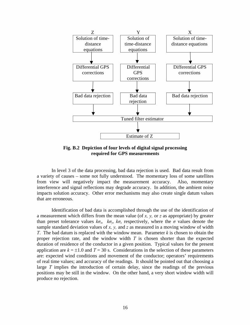
This is shown in Fig. B.2 as the first level of required digital processing. In the case of the application of DGPS measurements, the application of the correction signal from a base station receiver is also fundamental. This is shown in Fig. B.2 as a second level signal processing. The first and second levels of processing are done entirely by the GPS engine. The central focus of interest in the measurement of overhead transmission conductor sag is in the measurement of altitude, that is z(t).

16

Z Y X Solution of time-

distance equations

Solution of time-distance

equations

Solution of time-distance equations

Differential GPS corrections

Differential GPS

corrections

Differential GPS corrections

Bad data rejection Bad data rejection

Bad data rejection

Tuned filter estimator

Estimate of Z

Fig. B.2 Depiction of four levels of digital signal processing required for GPS measurements

In level 3 of the data processing, bad data rejection is used. Bad data result from

a variety of causes – some not fully understood. The momentary loss of some satellites from view will negatively impact the measurement accuracy. Also, momentary interference and signal reflections may degrade accuracy. In addition, the ambient noise impacts solution accuracy. Other error mechanisms may also create single datum values that are erroneous.

Identification of bad data is accomplished through the use of the identification of

a measurement which differs from the mean value (of x, y, or z as appropriate) by greater than preset tolerance values kσx, kσy, kσz respectively, where the σ values denote the sample standard deviation values of x, y, and z as measured in a moving window of width T. The bad datum is replaced with the window mean. Parameter k is chosen to obtain the proper rejection rate, and the window width T is chosen shorter than the expected duration of residence of the conductor in a given position. Typical values for the present application are k = ±1.0 and T = 30 s. Considerations in the selection of these parameters are: expected wind conditions and movement of the conductor; operators’ requirements of real time values; and accuracy of the readings. It should be pointed out that choosing a large T implies the introduction of certain delay, since the readings of the previous positions may be still in the window. On the other hand, a very short window width will produce no rejection.

17

The effect of the bad data rejection can be observed in Fig. B,3, which shows the cumulative distribution of the absolute value of the error computed from measurements taken for a set of known positions. The results depicted in Fig. B.3 were obtained experimentally using a 12 channel DGPS receiver at a surveyed position near Phoenix, AZ at about 359 m above mean sea level taking readings at the rate of one per second.

C

umul

ativ

e di

strib

utio

n (%

)

Bad data rejected (— )Raw data (- - -)

Absolute value of error (m)

Fig. B.3 Effect of bad data rejection

A fourth level of digital signal processing is depicted in Fig. B.2. Note that the

measurements are made at approximately 0.9 s intervals, and the measured data is available at discrete values of time. For this reason, it is convenient to refer to the measured set of data as x(k), y(k), z(k). The time measurement is not used in this application. Field trials of a prototype instrument indicate that errors in x and y often occur simultaneously with errors in z. This suggests that measured x and y could provide additional information for corrections in z. In this fourth level of signal processing, two different techniques have been tested: a least squares estimator (LSE) and an artificial neural network estimator (ANNE). Both are separately used as tuned filter estimators that are trained (tuned) using a known data set. Surveyed data are used to provide a set of [xk, yk, zk] data which are used to select parameters of the estimators such that the error in the known set is minimized. For testing purposes, the data set allows the comparison of estimated x, y, z to known values thereby providing an estimate of the instrument accuracy.

18

In trying to capture the nonlinear behavior of the error, the LSE adopted is

formulated as:

( ) ( ) ( ) ( ) ( ) ( ) ( ))z n Ax n By n Cz n Dx n Ey n Fz n= + + + + +2 2 2 where x(n), y(n), z(n) are the sampled readings at certain time that produce the corresponding vertical measurement estimation ( )nz) . Using the set of measurements x(n), y(n), z(n) taken for a set of known altitude zo and replacing ( )nz) with zo the above equation can be expressed in matrix form as,

Ζ ΧΘKnown =

where Θ = [ A B C D E F]T. The parameters [ A, B, C, D, E, F] are computed using simple state estimation (i.e., least squares parameter estimation). One formulation involves the Moore-Penrose pseudoinverse of the matrix X [10]. The ANNE is implemented using a time lag feed forward network [11]. In this configuration, contrary to the LSE, p previous readings of x, y and z are used to estimate z. A two-weighted layer network is used, consisting of h neurons in the hidden layer and one output layer. A sigmoid function, specifically the logistic function [11] is employed as the activation function of the hidden neurons, while the output neuron employs a linear function. The optimum values of p and h are determined in the tuning process. A schematic of the network is shown in Fig. B.4.

x(n-p)

y(n-p)

z(n-p)

x(n)

Inputlayer

)z (n)

Hiddenlayer

Outputneuron

.

.

y(n)..

z(n)..

.

.

.

.

Fig. B.4 ANN parameter estimator for correcting z(n) data from DGPS measurement

19

Some results of field testing and the details of the signal processing techniques described here are shown in the Appendix. Note that through the use of a least squares estimator, accuracy within 21.5 cm was obtained 70% of the time, and using an artificial neural network estimator, an accuracy of at least 19.6 cm is obtained for 70% of the time (see Table A1).

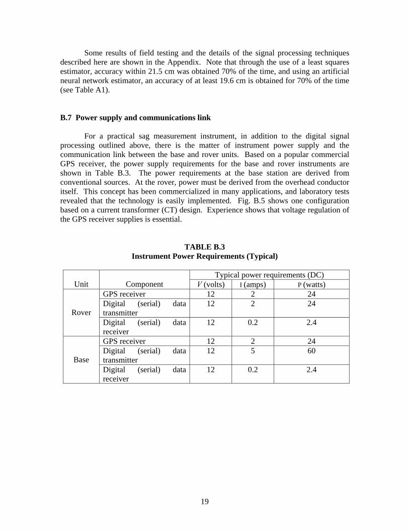
B.7 Power supply and communications link

For a practical sag measurement instrument, in addition to the digital signal processing outlined above, there is the matter of instrument power supply and the communication link between the base and rover units. Based on a popular commercial GPS receiver, the power supply requirements for the base and rover instruments are shown in Table B.3. The power requirements at the base station are derived from conventional sources. At the rover, power must be derived from the overhead conductor itself. This concept has been commercialized in many applications, and laboratory tests revealed that the technology is easily implemented. Fig. B.5 shows one configuration based on a current transformer (CT) design. Experience shows that voltage regulation of the GPS receiver supplies is essential.

TABLE B.3 Instrument Power Requirements (Typical)

Typical power requirements (DC)

Unit

Component V (volts) I (amps) P (watts) GPS receiver 12 2 24 Digital (serial) data transmitter

12 2 24

Rover Digital (serial) data receiver

12 0.2 2.4

GPS receiver 12 2 24 Digital (serial) data transmitter

12 5 60

Base Digital (serial) data receiver

12 0.2 2.4

20

PHASECONDUCTOR

CTCURRENT

VOLTAGEREGULATOR

12 VDC

Fig. B.5. Power supply for the rover unit: a magnetic ring is clamped around the conductor to be instrumented.

Communication between the rover and base station is accomplished using

standard digital communications technologies. A typical communication link consists of ‘on-off’ amplitude modulation for the communication channel, implemented in the Industrial Scientific and Medical (ISM) band, 902 - 928 MHz. The design tested in the laboratory is effectively a serial port connection via radio. Fig. B.6 shows a possible configuration. The frequency source in this design is derived from a voltage-controlled oscillator (VCO) that is held at the proper frequency by a phase locked loop circuit. The ultimate frequency source is a quartz crystal (XTAL).

An important issue in the present application is the performance of the

communication link in a high voltage environment (and, perhaps more serious, the 1.5 GHz band reception of the GPS signal at the rover). Experiments have been done to determine the difficulties in these areas and the main conclusion is that corona creates potentially intolerable conditions for radio reception in the 930 MHz and 1.5 GHz bands. There may also be some degree of ‘saturation’ in the receiver front end first stages, but the use of low noise amplifiers, standard in ISM and GPS technologies, seems to be adequate. It is important that the radio receivers at the rover be far from any corona. The receiver should be ‘shielded’ by instrument packaging that is smooth and corona free.

21

GPSRCVR

SERIALPORT

SHIFTREGISTER

AMPLMODULATOR

CLOCK

PHASELOCKEDLOOP

DIFFAMP FILTER VCO

XTAL

ANT ANDLOW NOISE AMPL

(a) GPS receiver/rover transmitter

LOWNOISEAMP

MIXER

VCO

PHASELOCKED

LOOPFILTER

FILTER AMP

SERIALPORT

GPSSOFTWARE

XTAL

(b) Base station receiver

Fig. B.6 Communication between the rover and base stations

B.8 Signal processing results

In order to test the above described signal processing procedures, a series of tests

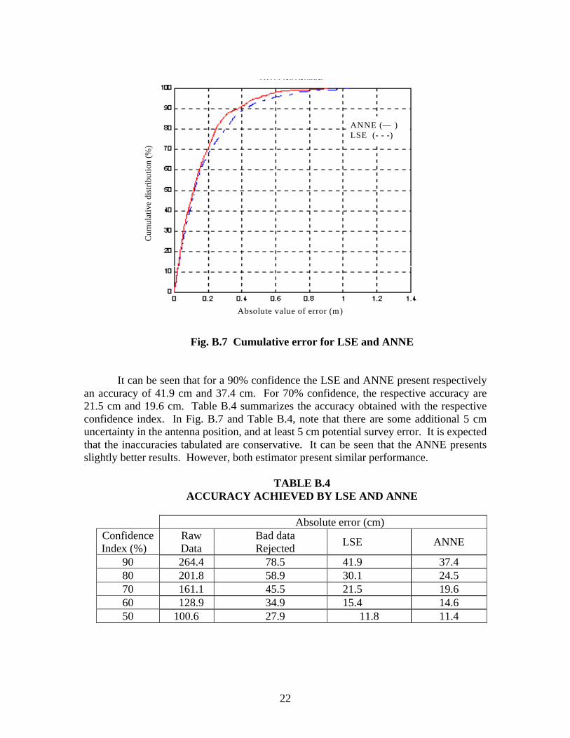
were done. One exemplar test is described as taking DGPS readings for ten known elevations (stations), collocated in longitude and latitude. The altitude difference between stations varies between 0.10 to 1.0 m. An average of 1,800 readings were taken for each station. From the ten stations, five were used to tune the estimators and the rest were used to test the performance of the estimators in the presence of data not previously seen. The bad data rejection in the third level has been computed using values of k = 1 and T = 30 s. These have presented a good performance regarding excessive number of data rejection and the response time, as explained previously. For the ANNE, several configurations have been explored regarding the number of neurons in the hidden layer. Good results were obtained for h = 4. In all cases, the number of previous readings used have been p = 9. With the configurations described the results obtained are summarized in Fig. B.7.

22

Cum

ulat

ive

dist

ribut

ion

(%)

Absolute value of error (m)

ANNE (— )LSE (- - -)

Fig. B.7 Cumulative error for LSE and ANNE

It can be seen that for a 90% confidence the LSE and ANNE present respectively an accuracy of 41.9 cm and 37.4 cm. For 70% confidence, the respective accuracy are 21.5 cm and 19.6 cm. Table B.4 summarizes the accuracy obtained with the respective confidence index. In Fig. B.7 and Table B.4, note that there are some additional 5 cm uncertainty in the antenna position, and at least 5 cm potential survey error. It is expected that the inaccuracies tabulated are conservative. It can be seen that the ANNE presents slightly better results. However, both estimator present similar performance.

TABLE B.4

ACCURACY ACHIEVED BY LSE AND ANNE

Absolute error (cm) Confidence Index (%)

Raw Data

Bad data Rejected LSE ANNE

90 264.4 78.5 41.9 37.4 80 201.8 58.9 30.1 24.5 70 161.1 45.5 21.5 19.6 60 128.9 34.9 15.4 14.6 50 100.6 27.9 11.8 11.4

23

B.9 Conclusions

The main conclusion of this study is that DGPS technology is feasible for the direct instrumentation of overhead power line conductor sag measurement. The accuracy of such an instrument is in the range of 19.6 cm 70% of the time. The method utilizes two GPS receivers, one as a base station which must be at an accurately surveyed location. The instrument can be designed such that the rover receiver operating power is taken from the line. Care must be taken in the design of the instrument package because of the potential of interference from corona. The main digital signal processing needed to obtain accurate z measurements are bad data rejection, least squares parameter estimation, or artificial neural network filtering.

Although the subject of dynamic line ratings is not considered here, it is believed

that real time sag measurement can be translated into real time dynamic circuit ratings, and this is expected to have value in the sale of transmission capacity.

References

[1] G. Ramon, IEEE Task Force Chairman: “Dynamic thermal line rating summary and status of the state-of-the-art technology,” IEEE Trans. Power Delivery, vol. PWRD-2, No. 3, pp. 851-856, July 1987.

[2] IEEE Standard for Calculating the Current-Temperature Relationship of Bare Overhead Conductors, IEEE Standard. 738-1993, New York, 1993.

[3] T. Seppa, “Accurate ampacity determination: temperature-sag model for operational real time ratings,” IEEE Trans. Power Delivery, vol. 10, No. 3, pp. 1460-1466, July 1995.

[4] U. Fernández, C. Mensah-Bonsu, J. Wells, G. Heydt, “Calculation of the maximum steady state transmission capacity of a system,” Proceedings of the 30th North American Power Symposium, Cleveland, Ohio, October 19-20, 1998, pp. 300-305.

[5] D. Douglas, A. Edris, “Real-time monitoring and dynamic thermal rating of power transmission circuits,” IEEE Trans. Power Delivery, vol. 11, No. 3, pp. 1407-1415, July 1996.

[6] B. J. Cory, P. F. Gale, "Satellites for power system applications," IEE Power Engineering Journal, vol. 7 No. 5, October 1993.

[7] J. Hurn, Differential GPS Explained, Trimble Navigation Ltd., Sunnyvale, CA 1993.

[8] E. Kaplan. Understanding GPS: Principles and Applications, 1996.

[9] T. Gray, NAVSTAR GPS and DGPS, CSI Inc., 1997.

[10] G. Heydt, Computer Analysis Methods for Power Systems, Stars in a Circle Publications, Scottsdale, AZ, 1998.

[11] S. Haykin, Neural Networks: A Comprehensive Foundation, 2nd Edition, Prentice Hall, New York, NY, 1999.

[12] D. G. Fink, H. W. Beaty (Editors), Standard Handbook for Electrical Engineers, 13th Edition, McGraw-Hill, 1993.