Advances in Quantifying Air-Sea Gas Exchange and Environmental Forcing ∗ Rik Wanninkhof, 1 William E. Asher, 2 David T. Ho, 3 Colm Sweeney, 4 and Wade R. McGillis 5 1 National Oceanographic and Atmospheric Administration/Atlantic Oceanographic and Meteorological Laboratory, Miami, Florida 33149; email: [email protected] 2 Applied Physics Laboratory, University of Washington, Seattle, Washington 98105; email: [email protected] 3 Department of Oceanography, University of Hawaii, Honolulu, Hawaii 96822; email: [email protected] 4 Global Monitoring Division, National Oceanographic and Atmospheric Administration/Earth Systems Research Laboratory, Boulder, Colorado 80305; email: [email protected] 5 Lamont-Doherty Earth Observatory of Columbia University, Palisades, New York 10964; email: [email protected] Annu. Rev. Mar. Sci. 2009. 1:213–44 First published online as a Review in Advance on September 19, 2008 The Annual Review of Marine Science is online at marine.annualreviews.org This article’s doi: 10.1146/annurev.marine.010908.163742 Copyright c 2009 by Annual Reviews. All rights reserved 1941-1405/09/0115-0213$20.00 ∗ The U.S. Government has the right to retain a nonexclusive, royalty-free license in and to any copyright covering this paper. Key Words gas fluxes, gas transfer velocity, carbon cycle, air-sea interaction Abstract The past decade has seen a substantial amount of research on air-sea gas ex- change and its environmental controls. These studies have significantly ad- vanced the understanding of processes that control gas transfer, led to higher quality field measurements, and improved estimates of the flux of climate- relevant gases between the ocean and atmosphere. This review discusses the fundamental principles of air-sea gas transfer and recent developments in gas transfer theory, parameterizations, and measurement techniques in the context of the exchange of carbon dioxide. However, much of this discussion is applicable to any sparingly soluble, non-reactive gas. We show how the use of global variables of environmental forcing that have recently become avail- able and gas exchange relationships that incorporate the main forcing factors will lead to improved estimates of global and regional air-sea gas fluxes based on better fundamental physical, chemical, and biological foundations. 213 Annu. Rev. Marine. Sci. 2009.1:213-244. Downloaded from arjournals.annualreviews.org by University of Massachusetts - Dartmouth on 01/05/09. For personal use only.

Welcome message from author
This document is posted to help you gain knowledge. Please leave a comment to let me know what you think about it! Share it to your friends and learn new things together.
Transcript

ANRV396-MA01-10 ARI 4 November 2008 8:3
Advances in QuantifyingAir-Sea Gas Exchangeand Environmental Forcing∗
Rik Wanninkhof,1 William E. Asher,2 David T. Ho,3
Colm Sweeney,4 and Wade R. McGillis5
1National Oceanographic and Atmospheric Administration/Atlantic Oceanographic andMeteorological Laboratory, Miami, Florida 33149; email: [email protected] Physics Laboratory, University of Washington, Seattle, Washington 98105;email: [email protected] of Oceanography, University of Hawaii, Honolulu, Hawaii 96822;email: [email protected] Monitoring Division, National Oceanographic and Atmospheric Administration/EarthSystems Research Laboratory, Boulder, Colorado 80305; email: [email protected] Earth Observatory of Columbia University, Palisades, New York 10964;email: [email protected]
Annu. Rev. Mar. Sci. 2009. 1:213–44
First published online as a Review in Advance onSeptember 19, 2008
The Annual Review of Marine Science is online atmarine.annualreviews.org
This article’s doi:10.1146/annurev.marine.010908.163742
Copyright c© 2009 by Annual Reviews.All rights reserved
1941-1405/09/0115-0213$20.00∗ The U.S. Government has the right to retain anonexclusive, royalty-free license in and to anycopyright covering this paper.
Key Words
gas fluxes, gas transfer velocity, carbon cycle, air-sea interaction
AbstractThe past decade has seen a substantial amount of research on air-sea gas ex-change and its environmental controls. These studies have significantly ad-vanced the understanding of processes that control gas transfer, led to higherquality field measurements, and improved estimates of the flux of climate-relevant gases between the ocean and atmosphere. This review discusses thefundamental principles of air-sea gas transfer and recent developments ingas transfer theory, parameterizations, and measurement techniques in thecontext of the exchange of carbon dioxide. However, much of this discussionis applicable to any sparingly soluble, non-reactive gas. We show how the useof global variables of environmental forcing that have recently become avail-able and gas exchange relationships that incorporate the main forcing factorswill lead to improved estimates of global and regional air-sea gas fluxes basedon better fundamental physical, chemical, and biological foundations.
213
Ann
u. R
ev. M
arin
e. S
ci. 2
009.
1:21
3-24
4. D
ownl
oade
d fr
om a
rjou
rnal
s.an
nual
revi
ews.
org
by U
nive
rsity
of
Mas
sach
uset
ts -
Dar
tmou
th o
n 01
/05/
09. F
or p
erso
nal u
se o
nly.
ANRV396-MA01-10 ARI 4 November 2008 8:3
INTRODUCTION
Air-sea gas exchange has been of intensive scientific interest for more than half a century be-cause of its importance in biogeochemical cycling of climate, weather, and health-related gaseouscompounds. In particular, gas exchange contributes to the mitigation of the anthropogenic green-house effect through absorption of excess atmospheric CO2 by the oceans. Gas exchange is alsoimportant to climate and atmospheric radiative transfer because of the sea-to-air flux of dimethyl-sulfide (DMS), which serves as a precursor to cloud condensation nuclei (CCN). CCN, in turn,are involved in radiative forcing through direct and indirect aerosol effects (Forster et al. 2007).In addition, oxygen levels in ocean surface waters are critically dependent on air-sea gas exchange,and the invasion of O2 can alleviate hypoxia in coastal oceans and estuaries. On local and regionalscales, the fate of volatile pollutants also depends on air-water gas exchange.
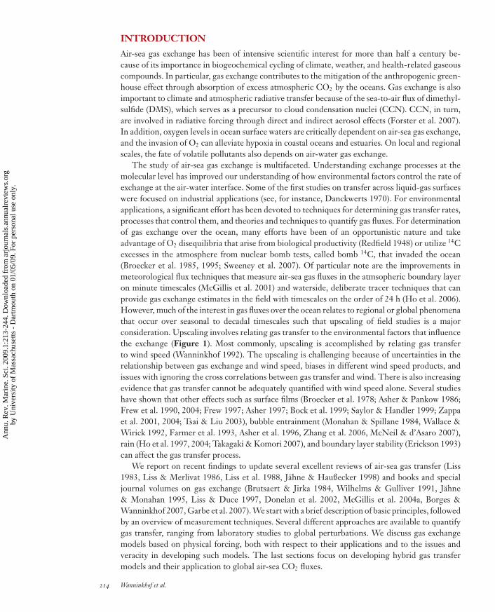
The study of air-sea gas exchange is multifaceted. Understanding exchange processes at themolecular level has improved our understanding of how environmental factors control the rate ofexchange at the air-water interface. Some of the first studies on transfer across liquid-gas surfaceswere focused on industrial applications (see, for instance, Danckwerts 1970). For environmentalapplications, a significant effort has been devoted to techniques for determining gas transfer rates,processes that control them, and theories and techniques to quantify gas fluxes. For determinationof gas exchange over the ocean, many efforts have been of an opportunistic nature and takeadvantage of O2 disequilibria that arise from biological productivity (Redfield 1948) or utilize 14Cexcesses in the atmosphere from nuclear bomb tests, called bomb 14C, that invaded the ocean(Broecker et al. 1985, 1995; Sweeney et al. 2007). Of particular note are the improvements inmeteorological flux techniques that measure air-sea gas fluxes in the atmsopheric boundary layeron minute timescales (McGillis et al. 2001) and waterside, deliberate tracer techniques that canprovide gas exchange estimates in the field with timescales on the order of 24 h (Ho et al. 2006).However, much of the interest in gas fluxes over the ocean relates to regional or global phenomenathat occur over seasonal to decadal timescales such that upscaling of field studies is a majorconsideration. Upscaling involves relating gas transfer to the environmental factors that influencethe exchange (Figure 1). Most commonly, upscaling is accomplished by relating gas transferto wind speed (Wanninkhof 1992). The upscaling is challenging because of uncertainties in therelationship between gas exchange and wind speed, biases in different wind speed products, andissues with ignoring the cross correlations between gas transfer and wind. There is also increasingevidence that gas transfer cannot be adequately quantified with wind speed alone. Several studieshave shown that other effects such as surface films (Broecker et al. 1978; Asher & Pankow 1986;Frew et al. 1990, 2004; Frew 1997; Asher 1997; Bock et al. 1999; Saylor & Handler 1999; Zappaet al. 2001, 2004; Tsai & Liu 2003), bubble entrainment (Monahan & Spillane 1984, Wallace &Wirick 1992, Farmer et al. 1993, Asher et al. 1996, Zhang et al. 2006, McNeil & d’Asaro 2007),rain (Ho et al. 1997, 2004; Takagaki & Komori 2007), and boundary layer stability (Erickson 1993)can affect the gas transfer process.
We report on recent findings to update several excellent reviews of air-sea gas transfer (Liss1983, Liss & Merlivat 1986, Liss et al. 1988, Jahne & Haußecker 1998) and books and specialjournal volumes on gas exchange (Brutsaert & Jirka 1984, Wilhelms & Gulliver 1991, Jahne& Monahan 1995, Liss & Duce 1997, Donelan et al. 2002, McGillis et al. 2004a, Borges &Wanninkhof 2007, Garbe et al. 2007). We start with a brief description of basic principles, followedby an overview of measurement techniques. Several different approaches are available to quantifygas transfer, ranging from laboratory studies to global perturbations. We discuss gas exchangemodels based on physical forcing, both with respect to their applications and to the issues andveracity in developing such models. The last sections focus on developing hybrid gas transfermodels and their application to global air-sea CO2 fluxes.
214 Wanninkhof et al.
Ann
u. R
ev. M
arin
e. S
ci. 2
009.
1:21
3-24
4. D
ownl
oade
d fr
om a
rjou
rnal
s.an
nual
revi
ews.
org
by U
nive
rsity
of
Mas
sach
uset
ts -
Dar
tmou
th o
n 01
/05/
09. F
or p
erso
nal u
se o
nly.

ANRV396-MA01-10 ARI 4 November 2008 8:3
Wind
u*
Variables
Atm. stability
Fetch
Wind direction
Surfactants
Microbreaking
Bubbles
SST
Transport
BiologySlope
Boundary
layer
dynamics
k ∆pCO2
Air-sea CO2 flux
Kineticforcing
Thermodynamicforcing
Figure 1Simplified schematic of factors that affect air-sea CO2 fluxes. On the left are environmental forcing factors(kinetic forcing) that control the gas transfer velocity, k, and the variables that influence the forcing. On theright are the factors that affect the air-sea pCO2 difference (thermodynamic forcing, see Equation 3), alsocalled thermodynamic driving potential.
BASIC PRINCIPLES
The flux of slightly soluble nonreactive gases across the air-sea interface, F ′ (mol m−2s−1), can bedefined as the product of a quantity called the gas transfer velocity, k (m s−1), and the concentrationdifference between the top and bottom of the liquid boundary layer,
F = k(Cw − Co ), (1)
where Co is the gas concentration at the water surface (mol m−3) and Cw is the gas concentrationin the well-mixed bulk fluid below (mol m−3). The gas transfer velocity is referred to as thekinetic forcing function, and the concentration difference is the thermodynamic driving potential(Figure 1). Assuming equivalence of chemical potential across the air-water phase boundary, Co isexpressed in terms of the concentration of the gas in the air, Ca (mol m−3), and the dimensionlessOstwald solubility coefficient α. Under this assumption, Equation 1 becomes
F = k(Cw − α Ca ), (2)
where by convention F is negative for a flux of gas from the atmosphere to the ocean. Often,Equation 2 is written such that the thermodynamic driving force is expressed in terms of thepartial pressure of the gas in air and water. In the case of CO2, exchange across the air-waterinterface (Equation 2) is
F = k Ko (pCO2w − pCO2a ), (3)
′For a complete list of symbols used in this article, please see Appendix A.
www.annualreviews.org • Quantifying Air-Sea Gas Exchange 215
Ann
u. R
ev. M
arin
e. S
ci. 2
009.
1:21
3-24
4. D
ownl
oade
d fr
om a
rjou
rnal
s.an
nual
revi
ews.
org
by U
nive
rsity
of
Mas
sach
uset
ts -
Dar
tmou
th o
n 01
/05/
09. F
or p
erso
nal u
se o
nly.
ANRV396-MA01-10 ARI 4 November 2008 8:3
where Ko (mol m−3 Pa−1) is the aqueous-phase solubility of CO2, pCO2a (Pa) is the partial pressureof CO2 in air, and pCO2w (Pa) is the partial pressure of CO2 in water. Assuming CO2 behavesas an ideal gas, Ko is related to α by Ko = α (R TW )−1, where R (m3 Pa K−1 mol−1) is the idealgas constant and TW (K ) is the water temperature. For sparingly soluble gases that are subjectto rapid chemical reaction in the aqueous phase (for instance, the air-water exchange of CO2 forpH > 10), Equation 2 must be modified as
F = kε (Cw − α Ca ), (4)
where ε is the chemical enhancement factor.Although the parameterizations for k discussed below are largely empirical in nature, provid-
ing a conceptual model for air-sea gas transfer aids in both understanding which environmentalforcings are most important and in relating gas transfer measurements made using one gas (forinstance, 222Rn) to a different gas (for instance, CO2) on the basis of the physicochemical prop-erties of the gases. Nearly all conceptual models for air-water transfer of slightly soluble (that is,α <≈ 5), nonreactive gases show that k is controlled by the aqueous-phase hydrodynamics verynear the air-water interface. The simplest of these is the stagnant-film model (Liss & Slater 1974),which proposes that the transfer process is rate limited by molecular diffusion through a thin layerof water with constant thickness at the air-water interface. From Fick’s first law of diffusion, k isthen equal to molecular diffusivity, D (m2 s−1), divided by the thickness of the stagnant film, δ (m).Therefore, processes that decrease δ will increase k.
Although appealing in its simplicity, stagnant-film theory is lacking because it does not providea complete physical picture of the transfer process. For example, laboratory and field studies haveshown that k is better modeled as being proportional to D to a fractional power between one-half and two-thirds (Ledwell 1984, Jahne et al. 1984, Upstill-Goddard et al. 1990, Nightingaleet al. 2000b). Although this discrepancy can be resolved through scaling arguments that suggestthat δ is proportional to D1/2 or D1/3 (Davies 1972) so that the ratio of D/δ has the observedfunctionality with respect to k, direct and indirect measurements of the gas concentrations verynear the water surface have shown that the near surface is poorly modeled as a stagnant layerwith constant thickness (Lee & Luk 1982, Luk & Lee 1986, Asher & Pankow 1989, Wolff &Hanratty 1994, Munsterer & Jahne 1998, Woodrow & Duke 2001, Takehara & Etoh 2002). Amore accurate conceptual model envisions the near-surface layer as dynamic, either with a variablethickness controlled by impinging eddies (Harriott 1962), flow divergences (Brumley & Jirka1988), or mixing with the bulk at frequent intervals through surface renewal events (Danckwerts1951). These more complex models predict that k will be proportional to D to a fractional powerbetween one-half and two-thirds, in agreement with the experimental results (for instance, Davieset al. 1964). Understanding the dependence of k on D is critical because there is a very limitednumber of gases suitable for use as tracers of the air-sea gas flux and, in many cases, the gasfor which F must be known cannot be measured directly. Thus, measurements of F made forone gas must be converted into the F for the gas of interest. Typically, this is done by using apredicted functional relationship between D and k to convert between k for two different gases.Development of accurate parameterizations of air-sea exchange that are applicable for a range ofgases must include the dependence of k on D.
A complete exposition of the range of conceptual models available for air-sea gas exchange isbeyond the scope of this review. However, one similar feature of these models is they predict thatk will be proportional to Dn where 1/2 < n < 2/3, depending on the assumptions made aboutthe details of the hydrodynamics in the near-surface aqueous layer and whether an eddy diffu-sion/boundary layer framework is adopted (for instance, Deacon 1977; Ledwell 1984; McCready& Hanratty 1984, 1985; Jahne et al. 1987; Brumley & Jirka 1988; Fairall et al. 2000; Banerjee et al.
216 Wanninkhof et al.
Ann
u. R
ev. M
arin
e. S
ci. 2
009.
1:21
3-24
4. D
ownl
oade
d fr
om a
rjou
rnal
s.an
nual
revi
ews.
org
by U
nive
rsity
of
Mas
sach
uset
ts -
Dar
tmou
th o
n 01
/05/
09. F
or p
erso
nal u
se o
nly.

ANRV396-MA01-10 ARI 4 November 2008 8:3
2004; Hara et al. 2007) or an eddy structure approach such as surface renewal or surface penetra-tion is used (Danckwerts 1951, Harriott 1962, Fortescue & Pearson 1967, Lamont & Scott 1970,Soloviev & Schlussel 1994, Zhao et al. 2003). These approaches all share a common detail that kis expressed in terms of the molecular diffusivity and some function based on the aqueous-phasehydrodynamics or characteristics of the aqueous boundary layer. This can be written as
k = a Dng(Q, L, ν), (5)
where a is a constant that is model dependent and g(Q, L, ν) represents a model-dependent functionbased on a velocity scale, Q (for instance, the turbulence intensity, water-side friction velocity u∗ ),a length scale, L (for instance, turbulence integral length scale, boundary layer depth), and thekinematic viscosity of water, ν. Typically, Equation 5 is modified in terms of the nondimensionalSchmidt number (Sc) (defined as Sc = ν/D) so that k becomes
k = aSc−n f (Q, L, ν). (6)
The parameterizations of k presented below are all derived empirically from this functional formbased on the assumption that the kinetic energy input to the water from the wind stress is funda-mental in driving air-water exchange. Because the energy input from the wind is known to increasenonlinearly with wind speed owing to wave generation and wave breaking (for instance, Craig &Banner 1994, Terray et al. 1996), parameterizations of k in terms of wind speed, U, propose that kwill increase in proportion to Um where m > 1, a conclusion that has been supported by laboratoryand field results.
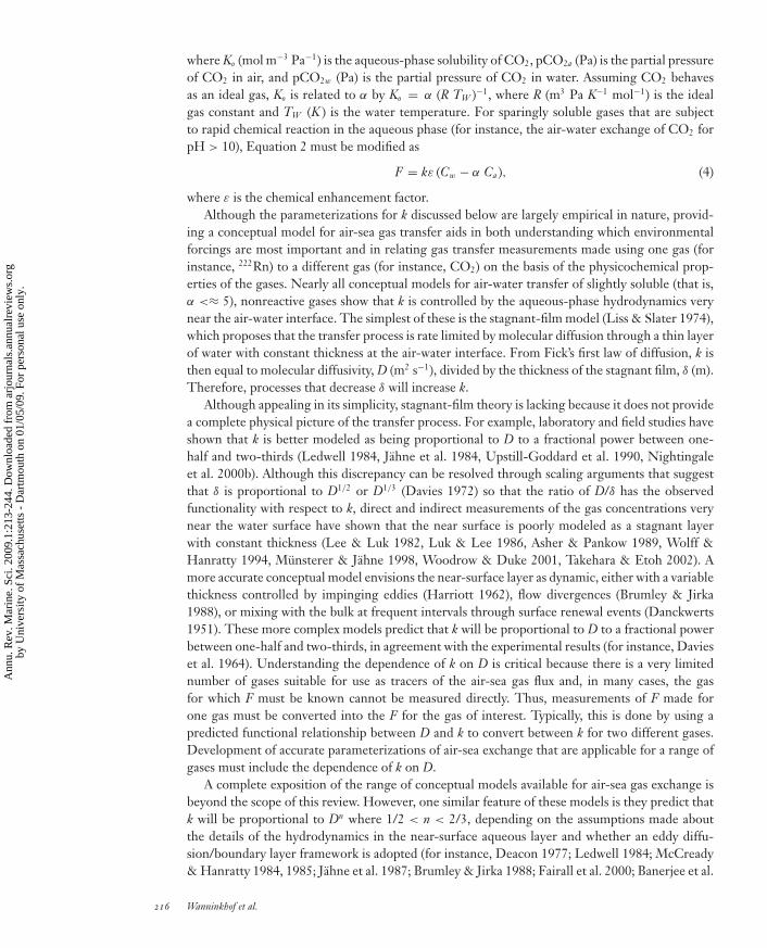
It should be noted that Equation 6 is not appropriate for expressing the transfer rate for solubleor reactive gases. The rate of transfer of gases with α > 100, or gases that rapidly react in water,is not controlled by hydrodynamic processes in the water side of the air-water interface (Liss &Slater 1974). Instead, k for these gases is controlled by air-side processes (Figure 2). Gases ofenvironmental interest that fall in this category include water vapor, ozone, ammonia, and sulfurdioxide. Limited studies performed with soluble gases show transfer velocities that are two to threeorders of magnitude higher than nonsoluble gases at a given U, and the functionality with respectto U is nearly linear (Liss 1983, Gallagher et al. 2001, Chang et al. 2004, McGillis et al. 2007).Gases with intermediate solubility exhibit both air-side and water-side resistance. For instance,DMS with α ≈ 10 is approximately 10% air-phase and 90% water-phase controlled (McGilliset al. 2000). A summary of D, Sc, and α values for select gases of environmental interest at 20◦Cin seawater is given in Table 1.
Whether a gas will be rate controlled in the air or water is most easily described in terms ofthe two-film model by Liss & Slater (1974). The total resistance to transfer is then the sum of theair and water resistances, and k is inversely proportional to the total resistance,
k−1 = (ka/α)−1 + (εkw)−1, (7)
where ka/α ( = 1/Rair with Rair as the air-side resistance) and εkw ( = 1/Rwater with Rwater as thewater-side resistance) are the gas transfer velocities of the gas through the diffusive sublayer layersin the air-side and water-side of the interface, respectively. On the basis of the two-film model, ka
and kw are roughly proportional to the ratio of D for the gas in air and water so that ka ≈ 100 kw.Therefore, the water phase and air phase resistance will be roughly equal if εα ≈ 100.
www.annualreviews.org • Quantifying Air-Sea Gas Exchange 217
Ann
u. R
ev. M
arin
e. S
ci. 2
009.
1:21
3-24
4. D
ownl
oade
d fr
om a
rjou
rnal
s.an
nual
revi
ews.
org
by U
nive
rsity
of
Mas
sach
uset
ts -
Dar
tmou
th o
n 01
/05/
09. F
or p
erso
nal u
se o
nly.
ANRV396-MA01-10 ARI 4 November 2008 8:3
Diffusive sublayer
Diffusive sublayer
Turbulent layer
(air)
Turbulent layer
(water)
αCa
Cw
Cw
αCa
Figure 2Conceptual view of boundary layer concentration profiles where the resistance to gas transfer is concentratedin the diffusive sublayers. On the left (blue line) is the concentration profile for an insoluble gas with theresistance in the aqueous-side diffusive sublayer. On the right (red line) is the profile for a soluble gas withresistance in the air-side diffusive sublayer. Soluble gases have an Ostwald solubility ≈>100.
MEASUREMENT TECHNIQUES
As described above, the k for CO2, kCO2 , can be determined from other gases through their Scnumber dependence. The measurement of gas transfer velocities and fluxes can be separated intoto three broad categories:
1. Measurement of F in the air above the sea surface and �C in the water to determine kusing Equation 1. These methods are referred to as direct flux measurements or micro-meteorological approaches and include covariance (or eddy correlation), eddy accumulation,atmospheric concentration profile, and inertial dissipation techniques.
2. Measurement of Ca (in air) and the change in Cw (in water) as a function of time. Assumingthe water volume and surface area are known, F is then equal to the change in Cw mul-tiplied by the ratio of the volume to the surface area. Then, k can be calculated with Ca
and Cw using Equation 1. These bulk concentration techniques include mass-balance andperturbation studies where the concentration of gases in air and water are out of equilibriumthrough biological consumption/production, water heating/cooling (N2, O2, CO2, noblegases), radioactive decay (222Rn), or by purposeful addition (3He, SF6).
3. Proxy techniques where a nongaseous tracer whose air-sea flux is more easily measured is usedas a surrogate for a gas using the principle that all air-water transfer is controlled by the near-surface hydrodynamics. In field applications, proxy methods are limited to thermographicmethods that use heat.
The mathematical formalism, application, merits, and drawbacks of each method are out-lined below. The assessment focuses on the challenges, but progress has been significant over
218 Wanninkhof et al.
Ann
u. R
ev. M
arin
e. S
ci. 2
009.
1:21
3-24
4. D
ownl
oade
d fr
om a
rjou
rnal
s.an
nual
revi
ews.
org
by U
nive
rsity
of
Mas
sach
uset
ts -
Dar
tmou
th o
n 01
/05/
09. F
or p
erso
nal u
se o
nly.

ANRV396-MA01-10 ARI 4 November 2008 8:3
Table 1 Diffusion coefficients, Schmidt numbers (Sc), and solubilities for select gases at 20◦C for salt water (S = 35‰)1
Gas Mol. weight (g mol−1) D (10−5 cm2 s−1) Sc α Comment3He 3 7.29 144 0.008 ≈1% less soluble than HeHe 4 6.36 165 0.008CH4 16 1.55 677 0.028Ne 20 3.33 315 0.009N2 28 1.57 670 0.012O2 32 1.78 589 0.025Ar 40 1.82 576 0.028CO2 44 1.59 660 0.727N2O 44 1.5 698 0.524(CH3)2S 62 1.14 918 12.73 DMS
Kr 84 1.51 694 0.050CCl2F2 121 0.86 1219 0.09 CFC-12
Xe 131 1.19 880 0.1CCl3F 137 0.94 1120 0.31 CFC-11
SF6 146 1.05 992 0.004
CCl4 154 0.82 1286 0.68CCl2FCClF2 187 0.68 1544 0.1 CFC-113
Rn 222 1.07 980 0.317
Heat — 1.75 6 —
1Values are from disparate sources and should be considered approximate (≈5%).
the past decade, and the new and improved techniques have improved our in situ capabilities todetermine k .
Direct Flux Measurements
The first successful direct flux measurements for CO2 from ships were performed in the late 1990s(McGillis et al. 2001). Detailed overviews of the direct flux techniques in air and applications canbe found in McGillis et al. (2001) and Fairall et al. (2000). Brief synopses of these works areprovided here.
Covariance technique. The covariance or eddy correlation technique is considered one of thepurest ways to determine F, because it does not rely on assumptions about gas properties orapproximations concerning the turbulent structure of the atmospheric boundary layer. However,it is one of the more challenging flux measurements to make in the field owing to small signal-to-noise ratios, which result from a very small signal and non-ideal measurement conditionsfound at sea (Fairall et al. 2000). In the covariance method, F can be directly measured from thegas concentration, c, and the vertical velocity, w, in the atmospheric boundary layer using theexpression
F = 〈c ′w′〉 + c w, (8)
where the primes indicate fluctuations about a mean value denoted by the “〈 〉.” The second termis mean velocity (of dry air) to maintain the density of dry air in the presence of latent and sensibleheat fluxes. Covariance flux systems have been used extensively to measure momentum and heat
www.annualreviews.org • Quantifying Air-Sea Gas Exchange 219
Ann
u. R
ev. M
arin
e. S
ci. 2
009.
1:21
3-24
4. D
ownl
oade
d fr
om a
rjou
rnal
s.an
nual
revi
ews.
org
by U
nive
rsity
of
Mas
sach
uset
ts -
Dar
tmou
th o
n 01
/05/
09. F
or p
erso
nal u
se o
nly.
ANRV396-MA01-10 ARI 4 November 2008 8:3
fluxes (for instance, Fairall et al. 1997). The greatest challenges to implementing the covariancemethod at sea for trace gases are as follows: rapid, high-precision measurement of atmosphericgas concentrations; correction of the measured fluxes for the covarying flux of water vapor andtemperature [that is, the Webb effect (Webb et al. 1980, Liu 2005)]; and contamination of theturbulent velocity record by platform motion and flow distortion around the platform. Becausethe signal-to-noise ratio is small in covariance flux measurements, the presence of an air-sea gasconcentration difference large enough that fluctuations in Ca are significantly larger than theprecision of the measurement technique is critical for the covariance method.
Although the covariance technique has been used routinely on fixed platforms for many years(for instance, Katsaros et al. 1987), including CO2 measurements ( Jacobs et al. 2002), routineopen-ocean applications of this technique for the measurement of turbulent fluxes from researchvessels (Fairall et al. 1997, Edson et al. 1998) have been made only in the past two decades. Inparticular, the measurement of the velocity components necessary to compute covariances is moredifficult because the motion of the platform impacts the actual velocity measurements of the air.This motion contamination must, therefore, be removed before the fluxes can be computed. Theresulting corrected wind velocity can then be used to compute the covariance fluxes. However,even if the platform motion is completely removed from the measured velocity, the accuracy ofvelocity estimates is influenced by flow distortion around the vessel.
The challenge in applying this technique to trace gases is the high sampling rate and highprecision required to constrain c′, which typically requires sampling at 2 Hz or greater, and therelatively small signal (concentration variations with high background values) for many trace gases.Typically, the required precision of c′ is at least two orders of magnitude greater than that of the air-sea gradient. With such stringent precision requirements, compounding factors such as platformmotion and high sensible and latent heat fluxes can bias velocity/gas concentration covariance fluxestimates. Covariance flux measurements have been successfully implemented on seagoing vesselsfor CO2, DMS, and O3. For CO2, the uncertainty is 2 mol m−2 year−1 (Fairall et al. 2000). Bycomparison, the average current oceanic CO2 uptake due to the anthropogenic CO2 pertubationis about 0.5 mol m−2 year−1. This illustrates that the current CO2 direct flux measurements arelimited to large CO2 source or sink regions. In contrast, DMS is highly supersaturated over mostof the ocean, and atmospheric concentrations are low, so the c′ will be correspondingly larger thanfor CO2, which improves the signal-to-noise ratio (Huebert et al. 2004, Blomquist et al. 2006).Uncertainty in DMS fluxes is estimated to be 15–20% for a one-hour measurement (Huebert et al.2004). Ozone fluxes (Lenchow et al. 1982) are large owing to the high solubility and reactivity ofozone in surface water, which again facilitates the measurements. However, the solubility of DMSand the reactivity of O3 do not make either of them perfect proxies for air-water exchange of CO2
or other sparingly soluble gases.Recently, covariance techniques have been proposed for the water mixed layer in rough seas
(d’Asaro & McNeil 2007). The longer time and length scales of turbulence alleviate the highsampling rate requirements. However, it is unclear if the criteria for the method, such as isotropicturbulence, are met in the water column, although the initial results look promising. Furtherresearch in performing covariance measurements in water is needed.
Relaxed eddy accumulation. The eddy accumulation (EA) method was developed for gasesfor which concentration measurements in air could not be performed at the required frequencyneeded for covariance measurements. The method relies on measuring the concentration of gasin the updraft and downdraft separately and is expressed mathematically as
F = bχσw(Cup − Cdown), (9)
220 Wanninkhof et al.
Ann
u. R
ev. M
arin
e. S
ci. 2
009.
1:21
3-24
4. D
ownl
oade
d fr
om a
rjou
rnal
s.an
nual
revi
ews.
org
by U
nive
rsity
of
Mas
sach
uset
ts -
Dar
tmou
th o
n 01
/05/
09. F
or p
erso
nal u
se o
nly.

ANRV396-MA01-10 ARI 4 November 2008 8:3
where σw is the standard deviation of vertical velocity and the coefficient bχ depends on thethreshold and characteristic length scales of turbulence (Businger & Delaney 1990; Nie et al.1995; Zemmelink et al. 2002, 2004). The experimental setup is comprised of an anemometer thatcan accurately measure the vertical component of the wind, which is connected to a valve thatcan selectively sample the gas in the net upward component (updraft) and downward component(downdraft) of the wind. The major technical challenge in EA is to accurately sample gas concen-trations specifically from updrafts and downdrafts. EA instruments generally utilize a thresholdvelocity range between the updraft and downdraft velocities, which is not sampled to avoid am-biguity and bias in sampling. These methods are appealing because high sampling rates for gasconcentrations are not required as in the covariance method, and it is possible to dry the airstreambefore gas sampling to eliminate the need to correct for density variations caused by water vaporand temperature (Webb et al. 1980, Liu 2005).
Other Direct Flux Measurement Techniques
Other direct flux measurement techniques such as the profile method and the inertial dissipationapproach rely heavily on similarity theory and scaling arguments that are commonly referred toas the Monin Obukov Similarity Theory (MOST). A comprehensive overview of how MOST isapplied to the determination of gas fluxes can be found in Fairall et al. (2000). Here we provide arudimentary conceptual explanation of the methods.
Profile Method. The profile method takes advantage of small concentration gradients in air thatresult from a net flux into or out of the water. The flux is the product of friction velocity in air,ua∗ , and the concentration gradient between heights z1 and z2 in the atmsopheric boundary layer,divided by a transfer resistance, R1,2, between the heights of measurement (Roether 1983):
F = ua∗(Cz1 − Cz2)(R1,2)−1. (10)
Under neutral boundary conditions,
R1,2 = κ−1 ln(z2/z1), (11)
where κ is the Von Karman constant (≈0.4). A detailed description of the profile method with thetheoretical foundation, including approximations for stable and unstable boundary conditions,can be found in McGillis et al. (2001) and Edson et al. (2004). The profile technique in theatmosphere requires the use of MOST for stable and unstable boundary layers. For this discussion,the simplified formulas listed in Equation 10 and Equation 11 suffice to show that measurementheights are a determining factor for the precision of the measurement. The transfer resistancescales with the natural log of the difference in measurement height in air such that it is advantageousto get the first measurement close to the surface.
Because the atmospheric profile method relies on mean gradients in the boundary layer, it offersseveral advantages over other direct flux measurement techniques. Many gases cannot be measuredat rates that are high enough for eddy correlation because most gas measurement techniques relyon slow procedures that can also smear the high-frequency response (for instance, owing to watervapor removal and “dead volumes” en route to mass spectrometric and/or in gas chromatographicsample cells).
There are several requirements for the atmospheric profile technique to provide accurate fluxes.The surface momentum and buoyancy fluxes must be controlling the flow, and the parameter-izations become invalid when, for instance, surface waves and larger-scale processes influencethe near-surface properties. In addition, a number of fundamental assumptions such as surface
www.annualreviews.org • Quantifying Air-Sea Gas Exchange 221
Ann
u. R
ev. M
arin
e. S
ci. 2
009.
1:21
3-24
4. D
ownl
oade
d fr
om a
rjou
rnal
s.an
nual
revi
ews.
org
by U
nive
rsity
of
Mas
sach
uset
ts -
Dar
tmou
th o
n 01
/05/
09. F
or p
erso
nal u
se o
nly.
ANRV396-MA01-10 ARI 4 November 2008 8:3
homogeneity, stationarity, and turbulent kinetic energy balance are required. The correction foratmospheric stability is very close to those used for profiles measured over land (Edson et al. 2004).Because of the relatively small vertical gradients of trace atmospheric gases, the signal levels canbe close to or less than the gas detection noise level. In addition, displacements of the air intakeand instruments due to the motion of the ship are problematic owing to the nonlinear natureof the vertical gas gradient. The flow distortion may significantly modify the profile of the gasconcentration that is required for the flux computation. Finally, small-scale (≈<100 m) variationsin air-sea fluxes can cause variability in air concentrations in the footprint of measurement, whichcompromises the technique.
All the direct flux techniques measure surface fluxes rather than k. The k can be determined fromknowledge of the air-water concentration difference (see Equation 2), which requires knowledge ofthe footprint of the flux measurement. The footprint is the region over which the flux emanates anddepends on the height of measurement and boundary layer stability (Businger & Delaney 1990).For a measurement at 10-m height, the footprint ranges from 100 m to 20 km, with the largerfootprint applicable to stable boundary layer conditions. Thus, comprehensive measurements ofsurface water gas concentrations in the footprint are essential for robust k estimates from directflux techniques.
Mass Balance Techniques
These methods rely on measuring the rate of concentration change due to air-sea gas transferto equilibrium conditions after a perturbation of the gases in water. The basic principle can begleaned from Equation 2 and, recognizing that in the case where water volume exposed to theatmosphere is constant, F equals the change in mass of gas, M, divided by the surface area, A,
F = ∂M/∂tA−1. (12)
Thus, F can be determined and k can be estimated if the air-water concentration difference and massdecrease over time is known and well characterized. Several different methods of concentrationperturbation can be utilized.
Natural perturbations (oxygen and radon). The first estimates of gas transfer in the ocean(embayments) were performed with O2, taking advantage of disequilibria caused by temperaturechange or biological production and consumption (Redfield 1948). From changes in Cw for O2
over time, the total change in mass of water volume exposed to the atmosphere is determined.The change in mass due to the air-sea flux (FO2 ) and with sources or sinks other than the air-seaflux (S) can be expressed as
FO2 + SO2 = ∂M/∂tA−1. (13)
The key is to adequately constrain S, which is often the largest source of uncertainty in such mea-surements. The flux estimate for O2 based on changes in temperature of the water, in the absenceof biological productivity, can often be determined more accurately because the temperature de-pendence of solubility of the gases is well known. The driving force for gas transfer in this case isthe change in equilibrium due to changes in the αCa term in Equation 2. Although Ca for oxygenis constant as far as gas transfer is concerned, changes in α with temperature will change Co inEquation 1. Regional gas transfer velocities of O2 have been estimated by this approach throughthe use of global numerical models (Najjar & Keeling 1997).
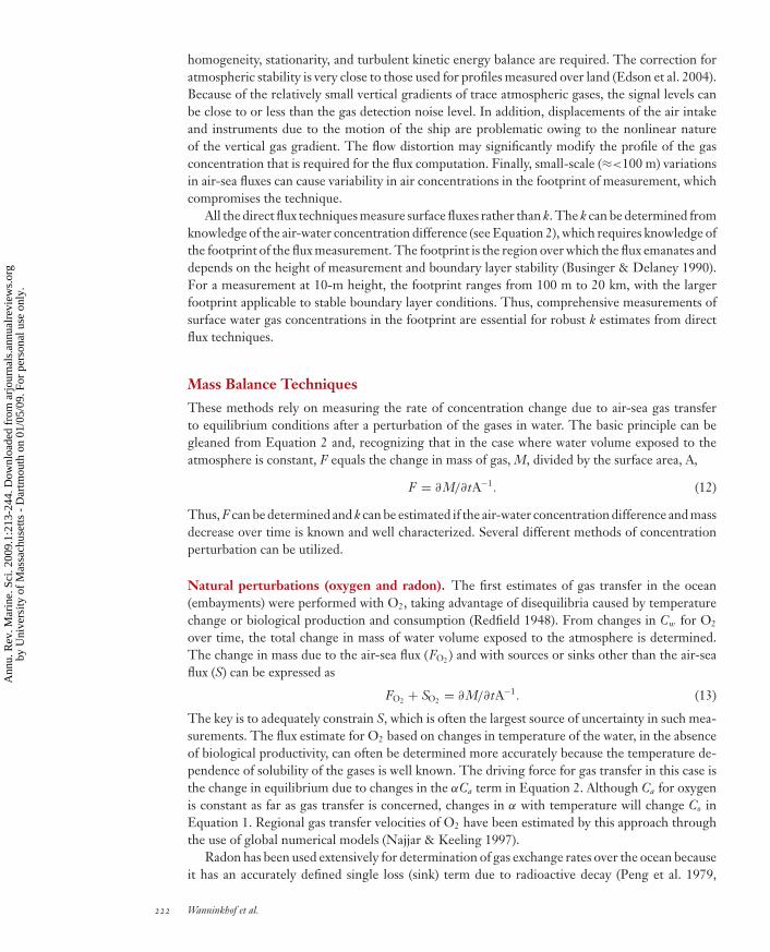
Radon has been used extensively for determination of gas exchange rates over the ocean becauseit has an accurately defined single loss (sink) term due to radioactive decay (Peng et al. 1979,
222 Wanninkhof et al.
Ann
u. R
ev. M
arin
e. S
ci. 2
009.
1:21
3-24
4. D
ownl
oade
d fr
om a
rjou
rnal
s.an
nual
revi
ews.
org
by U
nive
rsity
of
Mas
sach
uset
ts -
Dar
tmou
th o
n 01
/05/
09. F
or p
erso
nal u
se o
nly.
ANRV396-MA01-10 ARI 4 November 2008 8:3
Smethie et al. 1985). In short, in the absence of gas transfer the 222Rn gas will be in equilibriumwith its parent, 226Ra, in terms of activity, which is what is observed below the surface water mixedlayer. Within the water mixed layer, some of the 222Rn will escape owing to gas transfer such thatthe magnitude of disequilibrium of 222Rn and 226Ra in the mixed layer is directly proportional tothe gas transfer rate. The pertinent equations to determine the gas transfer velocity are derivedfrom Equation 2,
F222Rn = k(222Rnw − α222Rna ) ≈ k(222Rnw). (14)
Here, the concentration of 222Rn in the atmosphere is assumed to be zero. If the system is insteady state (stationary and homogeneous conditions in the water mixed layer), the loss due toradioactive decay must equal the flux
F222Rn = λI, (15)
where λ is the decay constant (2.1 10−6 s−1 or 0.18 day−1) and I is the deficit of 222Rn relative to226Ra in the mixed layer (in terms of activity, A) such that k = λI/A222Rnw.
The response time of the method will be directly proportional to the half-life of 222Rn of fourdays. Several large-scale ocean surveys and process studies have been performed to determine thegas transfer velocity with radon (Peng et al. 1979, Kromer & Roether 1983). Although basin-scale averages are in accord with other estimates, no clear relationship with wind was observed.Kromer & Roether (1983) provide a critical analysis of the uncertainties in the 222Rn methods andguidelines for how an optimal 222Rn gas exchange study in the ocean should be performed.
As with all mass balance techniques, gas exchange versus wind relationships with radon andoxygen are confounded by variability in two very important variables. The first is mixed layer depth,because changes in mixed layer depth will effectively change the mass, M, exposed to surface A(Equation 12). Regions with large gradients below the mixed layer will respond to changes in themixed layer depth due to entrainment, with episodic shifts in surface concentration that may notbe reflected in one-time concentration profiles in the water column. The second variable is shiftsin wind speed over the course of the observation. Again, instantaneous observations of wind speedhave often been used to calculate gas exchange using radon when it would be more appropraite tocompare a weighted distribution of wind approximately two weeks prior to measuring the radonprofile.
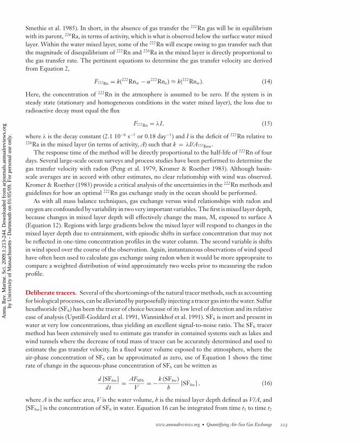
Deliberate tracers. Several of the shortcomings of the natural tracer methods, such as accountingfor biological processes, can be alleviated by purposefully injecting a tracer gas into the water. Sulfurhexafluoride (SF6) has been the tracer of choice because of its low level of detection and its relativeease of analysis (Upstill-Goddard et al. 1991, Wanninkhof et al. 1991). SF6 is inert and present inwater at very low concentrations, thus yielding an excellent signal-to-noise ratio. The SF6 tracermethod has been extensively used to estimate gas transfer in contained systems such as lakes andwind tunnels where the decrease of total mass of tracer can be accurately determined and used toestimate the gas transfer velocity. In a fixed water volume exposed to the atmosphere, where theair-phase concentration of SF6 can be approximated as zero, use of Equation 1 shows the timerate of change in the aqueous-phase concentration of SF6 can be written as
d [SF6w]dt
= AFSF6
V= −k (SF6w)
h[SF6w] , (16)
where A is the surface area, V is the water volume, h is the mixed layer depth defined as V/A, and[SF6w] is the concentration of SF6 in water. Equation 16 can be integrated from time t1 to time t2
www.annualreviews.org • Quantifying Air-Sea Gas Exchange 223
Ann
u. R
ev. M
arin
e. S
ci. 2
009.
1:21
3-24
4. D
ownl
oade
d fr
om a
rjou
rnal
s.an
nual
revi
ews.
org
by U
nive
rsity
of
Mas
sach
uset
ts -
Dar
tmou
th o
n 01
/05/
09. F
or p
erso
nal u
se o
nly.

ANRV396-MA01-10 ARI 4 November 2008 8:3
and rearranged to yield
k (SF6) = − h�t
ln(
[SF6w]t2
[SF6w]t1
), (17)
where �t = t2 – t1. Thus, k can be determined from the change in natural log of [SF6w] over time,provided h is known.
For the open ocean, the decrease in (SF6w) will occur through gas exchange and by advectionand dispersion. Thus, the surface area and volume exposed to the atmsophere will change. In thesecases, a second tracer is necessary. Although a nonvolatile tracer would be advantageous for thispurpose, because its decrease in concentration over time would be affected only by advection anddispersion, no tracer with the appropriate detection limit that is adequately inert has been foundfor large-scale ocean work.
For large-scale work, a clever alternative has been found in which two gases with differentdiffusion coefficients are used, namely 3He and SF6 (Watson et al. 1991, Wanninkhof et al. 1993).The light isotope of helium, 3He, meets the same criteria of inertness, low background, andlow detection limits as SF6. 3He has a Sc number that is eight times smaller than SF6. Whenthe two gases are released in a constant ratio, their concentration decrease in the water columndue to dispersion will be the same but the loss due to gas exchange will be different and thisdifference will be proportional to the inverse square root of the ratio of their respective Sc numbers:(Sc3He/ScSF6)−1/2 (i.e., 3He will be removed more quickly by gas exchange than SF6 because ittransfers three times faster through the water surface). The gas transfer velocity of 3He, k(3He)can then be expressed as
k(3He) = −h�t
�
{ln
([3He][SF6]
)}{1 −
[Sc(3He)Sc(SF6)
]1/2}−1
, (18)
where the delta term in braces represents the change in the logarithm of the ratio of the gasconcentrations over the time interval �t. 3He is one of the few gases that will work in combinationwith SF6 for this application, because the Sc numbers for other candidate gases are similar to thatof SF6 (Table 1).
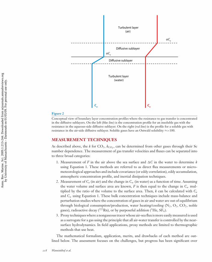
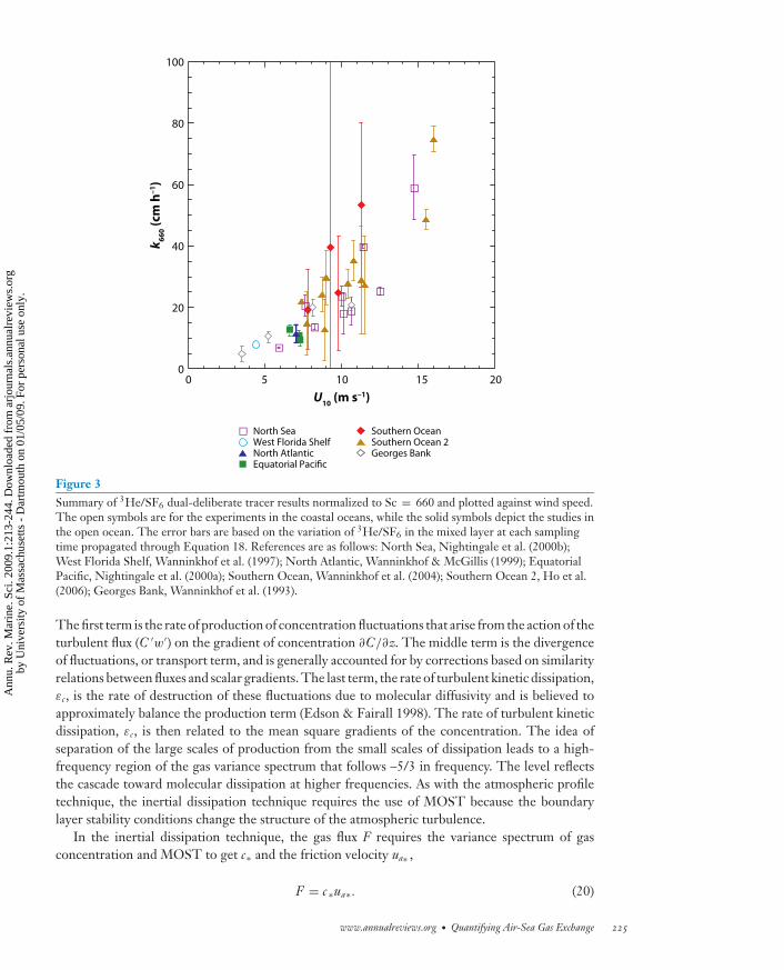
Successful 3He/SF6 studies have been performed in several different ocean basins under a rangeof conditions (Nightingale et al. 2000b, Ho et al. 2006, Wanninkhof et al. 2004). The time intervalto determine k will depend on the rate of gas transfer and mixed layer depth, and ranges fromone to four days. Results of most dual deliberate tracer studies over the ocean plotted versus windspeed are shown in Figure 3.
Proxy Techniques
Inertial dissipation method. The challenges associated with the eddy correlation method for theestimation of fluxes at sea have led to the use of the inertial dissipation method in the atmosphericboundary layer (Fairall & Larsen 1986). The method assumes an approximate balance of thegeneration and dissipation of turbulent fluctuations of the concentration of the gas whose flux isto be measured. This method is based on MOST for the high-frequency portion of the variance,or concentration fluctuation, spectrum. The method has been used extensively to measure dragcoefficients over the open ocean (Yelland et al. 1994).
The concentration variance budget in the atmospheric boundary layer can be expressed as
−C ′w′(
∂C∂z
)− 1
2∂C ′2w
∂z= εc . (19)
224 Wanninkhof et al.
Ann
u. R
ev. M
arin
e. S
ci. 2
009.
1:21
3-24
4. D
ownl
oade
d fr
om a
rjou
rnal
s.an
nual
revi
ews.
org
by U
nive
rsity
of
Mas
sach
uset
ts -
Dar
tmou
th o
n 01
/05/
09. F
or p
erso
nal u
se o
nly.
ANRV396-MA01-10 ARI 4 November 2008 8:3
00 5 10 15 20
20
40
60
80
100
North SeaWest Florida ShelfNorth AtlanticEquatorial Pacific
Southern Ocean Southern Ocean 2Georges Bank
U10
(m s–1)
k 66
0 (
cm h
–1)
Figure 3Summary of 3He/SF6 dual-deliberate tracer results normalized to Sc = 660 and plotted against wind speed.The open symbols are for the experiments in the coastal oceans, while the solid symbols depict the studies inthe open ocean. The error bars are based on the variation of 3He/SF6 in the mixed layer at each samplingtime propagated through Equation 18. References are as follows: North Sea, Nightingale et al. (2000b);West Florida Shelf, Wanninkhof et al. (1997); North Atlantic, Wanninkhof & McGillis (1999); EquatorialPacific, Nightingale et al. (2000a); Southern Ocean, Wanninkhof et al. (2004); Southern Ocean 2, Ho et al.(2006); Georges Bank, Wanninkhof et al. (1993).
The first term is the rate of production of concentration fluctuations that arise from the action of theturbulent flux (C ′w′) on the gradient of concentration ∂C/∂z. The middle term is the divergenceof fluctuations, or transport term, and is generally accounted for by corrections based on similarityrelations between fluxes and scalar gradients. The last term, the rate of turbulent kinetic dissipation,εc, is the rate of destruction of these fluctuations due to molecular diffusivity and is believed toapproximately balance the production term (Edson & Fairall 1998). The rate of turbulent kineticdissipation, εc, is then related to the mean square gradients of the concentration. The idea ofseparation of the large scales of production from the small scales of dissipation leads to a high-frequency region of the gas variance spectrum that follows –5/3 in frequency. The level reflectsthe cascade toward molecular dissipation at higher frequencies. As with the atmospheric profiletechnique, the inertial dissipation technique requires the use of MOST because the boundarylayer stability conditions change the structure of the atmospheric turbulence.
In the inertial dissipation technique, the gas flux F requires the variance spectrum of gasconcentration and MOST to get c∗ and the friction velocity ua∗ ,
F = c ∗ua∗. (20)
www.annualreviews.org • Quantifying Air-Sea Gas Exchange 225
Ann
u. R
ev. M
arin
e. S
ci. 2
009.
1:21
3-24
4. D
ownl
oade
d fr
om a
rjou
rnal
s.an
nual
revi
ews.
org
by U
nive
rsity
of
Mas
sach
uset
ts -
Dar
tmou
th o
n 01
/05/
09. F
or p
erso
nal u
se o
nly.

ANRV396-MA01-10 ARI 4 November 2008 8:3
By equating dissipation to generation and knowing the dependence of the overall gradient ofconcentration, the gas transfer rate may be determined. Some work has been done in applyingthis method to gas fluxes over the ocean for CO2 (Larsen et al. 1997). The main attraction ofthe inertial dissipation method is its use of the high-frequency portion of the spectrum whereplatform motions are much smaller than the turbulence signal. Thus, ship motion corrections andprecise vertical alignments are not required. However, the inertial subrange occurs at frequencieshigher than the upper frequency limit of the covariance method, so this method requires a veryfast sensor response and the requirements for low sensor noise are more critical.
Heat. Heat is an attractive proxy tracer of air-water gas exchange because temperature can bemeasured with high accuracy and very good temporal resolution ( Jahne et al. 1989), thus allowingthe details of air-water exchange to be studied. With the advent of infrared (IR) imagers, especiallythose equipped with focal plane arrays, several so-called IR thermographic techniques have beendeveloped that allow the spatial details of air-water heat exchange to be measured with unprece-dented spatial and temporal resolution (Haußecker & Jahne 1995; Haußecker et al. 1995, 2002;Garbe et al. 2004; Schimpf et al. 2004).
The use of IR thermographic methods for the study of gas transfer relies on the assumptionthat the net flux of heat and the resulting transfer velocity, k(heat), can be related to an equivalentvalue for gas via the use of a diffusivity scaling based on Equation 6. Although initial applications ofthe technique indicated that this scaling worked and a direct equivalence existed between k(heat)and k(gas) ( Jahne et al. 1989, Haußecker et al. 1995), more recent use of heat as a proxy tracerhas indicated that the relationship might not be as straightforward as implied by Equation 6. Inparticular, Zappa and coworkers (2004), Atmane and coworkers (2004), and Asher and coworkers(2004) all find that when scaled according to Equation 6, k(heat) measured by the active infraredtechnique developed by Haußecker and colleagues (1995) overpredicts k(gas) by a factor of two tothree. Similarly, Garbe and coworkers (2004) find a scale factor of 1.3 between k(heat) and k(gas).Atmane and coworkers (2004) explain this scale factor as a result of the interplay between thedistance at which water-side turbulence eddies approach the interface and the order of magnitudedifference in diffusive length scales between heat and gas. There is scientific debate as to whetherthermographic techniques provide a means for definitive quantification of k(gas), and a clearresolution to this problem is not available at present. However, whatever the final resolution ofthe question of a direct equivalence between k(heat) and k(gas), it is clear that IR imagery providesa unique means to visualize the microscale wave breaking, coherent motions, and aqueous-phaseturbulence occurring very near the water surface.
RECENT FIELD STUDIES THAT UTILIZE IMPROVEDMEASUREMENT TECHNIQUES
Major advances have been made in determining k over the ocean in several large field campaignssuch as the GasEx-98 and GasEx-2001 studies (McGillis et al. 2001, 2004b), the Air-Sea GasExchange/Marine Aerosol and Gas Exchange (ASGAMAGE) field program ( Jacobs et al. 2002),and the Surface Ocean Lower Atmosphere Study (SOLAS) Air-Sea Gas Exchange (SAGE) ex-periment (Ho et al. 2006). These studies successfully addressed the challenges outlined above.For direct flux measurements, improvements include accurate correction for the ship’s motion(Edson et al. 1998), improved sensor resolution, accurate assessments of Webb corrections, andperforming studies in regions with a sufficient concentration gradient to improve the signal-to-noise ratio. These studies have dealt with all the shortcomings of the direct flux techniques outlinedin Broecker et al. (1986). New analysis techniques have facilitated DMS flux measurements from
226 Wanninkhof et al.
Ann
u. R
ev. M
arin
e. S
ci. 2
009.
1:21
3-24
4. D
ownl
oade
d fr
om a
rjou
rnal
s.an
nual
revi
ews.
org
by U
nive
rsity
of
Mas
sach
uset
ts -
Dar
tmou
th o
n 01
/05/
09. F
or p
erso
nal u
se o
nly.
ANRV396-MA01-10 ARI 4 November 2008 8:3
ships (Huebert et al. 2004). Although errors in individual 10–30 min direct flux measurementsstill are 50–100%, the effective use of statistical approaches, with the large numbers of observa-tions such as bin averaging in discrete wind speed ranges, has decreased the uncertainty in binnedmeasurements to 10% over two to four weeks of sampling.
Determination of k from water column mass balance estimates is now almost exclusively doneby dual-deliberate tracer methods that use 3He and SF6. Improved accuracy and speed of analysisof SF6, an increased number of measurements of 3He at shoreside laboratories, and improvedsampling protocols have all contributed to greater accuracy of the measurements. The uncertaintyof the measurements is a direct function of measurement interval; longer intervals lead to greaterdecreases in ratios (Equation 18) but also generally lead to integration over larger ranges of windspeed. Accurate determination of ratio decrease depends on good estimates of the mixed layerdepth. Precisions of better than 10% over one- to two-day intervals have been achieved by thedual tracer method over the ocean (Ho et al. 2006). Studies relating the dual tracer results to othergases have been performed (Asher & Wanninkhof 1998), but additional efforts are warrantedconsidering the increased use of this approach. These additional efforts are necessary because forCO2, sea spray and bubble injection due to breaking waves and to a lesser extent to rainfall mayaffect the dependence of k on Sc number given in Equation 18.
FORCING
Most determinations of gas transfer velocities are complex and require dedicated field studies. Toutilize the gas transfer velocities to determine regional or global fluxes through bulk formulationssuch as given in Equation 1, the measurements must be scaled up and/or parameterized with forcingfunctions that can be readily determined. Here, we first describe gas transfer and forcing over asmooth or undulated surface, and then extend it to situations where bubbles affect the exchange.
The general expression for gas transfer is given by Equation 6. Relating the function f (Q, L,ν) to environmental forcing becomes the key issue. Based on analogous behavior between heat,momentum, and gas, the surface friction velocity in water, uw∗ , is a critical parameter ( Jahne et al.1987). Deacon (1977) proposed a general formulation for k in the case of an aerodynamicallysmooth surface,
k = β−1uw∗ Sc−n, (21)
where β is a numerical constant determined from classical boundary layer theory. Although thisrepresentation can account for shear-induced turbulence in the absence of waves, it is not appro-priate when there is significant contribution to the net stress from breaking and nonbreaking wavesor when other drivers such as bubble entrainment, rain, and buoyancy-generated turbulence aresignificant.
An alternative approach is to establish a formulation that includes most parameters known toaffect gas exchange. This was performed by Fairall and coworkers (2000) and Hare and coworkers(2004) and leads to the following expression for sparingly soluble gases with liquid-side control:
k = ua∗[(ρw/ρa )−1/2(hw Sc1/2w + ln(zw/dw)/κ)]−1, (22)
where subscripts w and a refer to the water and air phase, respectively, and ρa and ρw are thedensity of air and water, respectively. hw = �Rr
1/4/ϕ, where � is an adjustable parameter, Rr is theroughness Reynolds number, and ϕ is an empirical function that accounts for buoyancy effects onturbulent transfer. Many of the variables in Equation 22 can be estimated from knowledge of air andwater temperature, sea surface skin temperature, salinity, net long-wave and short-wave radiation,wind speed, relative humidity, and atmospheric pressure. However, the absolute magnitudes of
www.annualreviews.org • Quantifying Air-Sea Gas Exchange 227
Ann
u. R
ev. M
arin
e. S
ci. 2
009.
1:21
3-24
4. D
ownl
oade
d fr
om a
rjou
rnal
s.an
nual
revi
ews.
org
by U
nive
rsity
of
Mas
sach
uset
ts -
Dar
tmou
th o
n 01
/05/
09. F
or p
erso
nal u
se o
nly.

ANRV396-MA01-10 ARI 4 November 2008 8:3
the fluxes are determined from fitting results from field studies. The integrated model developedby Hare and coworkers (2004) includes the effect of bubbles on k, which are added as a separatecomponent (see below). The parameters included in Equation 22 clearly indicate that simpleequations that relate gas transfer with wind lack the full range of parameters that affects gas transfer.
Relationships of Gas Exchange With Wind
Many factors can affect gas transfer, but over the global ocean wind forcing has a dominanteffect. This phenomenon has a theoretical foundation based on the relationship of k and u∗ (seeEquations 21 and 22) and the relationship between wind and friction velocity, which under neutralatmospheric conditions is
U10 = (ρw/ρa )1/2uw∗C−1/2d , (23)
where Cd is the drag coefficient that is related to the surface roughness. The uw∗ is the frictionvelocity in water and is related to the friction velocity in air, ua∗ , through uw∗ = (ρa/ρw)1/2 ua∗ .
Although theoretical relations between U10 and uw∗ exist for all atmospheric stabilities, mostrelationships of k with wind are empirical. The first successful studies that related gas exchange towind were performed in wind-wave tunnels followed by deliberate tracer studies in lakes. Althougha general trend of k increasing with increases in U10 was observed over the ocean with the massbalance techniques that use O2 and 222Rn, it was not until the advent of the dual deliberate tracermethods that clear patterns of gas transfer with wind over the ocean were observed (Figure 3).
The first popular gas exchange–wind speed parameterization was derived from conceptualand theoretical considerations adjusted to the natural environment. On the basis of theoreticalarguments and wind-wave tanks results, Liss & Merlivat (1986) assumed three linear segments ofgas transfer with wind: the smooth regime, a regime with an undulating surface, and a regime withbreaking waves. The relationship for the undulating regime Equation 25 was adjusted so that k600
matched the first deliberate tracer results from lakes (Wanninkhof et al. 1985),
k600 = 0.17 U10 (U10 < 3.6 m s−1), (24)
k600 = 2.85 U10 − 9.65 (3.6 < U10 < 13 m s−1), (25)
k600 = 5.9 U10 − 49.3 (U10 > 13 m s−1), (26)
where 600 in k600 refers to the Sc of CO2 at 20◦C for fresh water. The k600 (and k660 below) areexpressed in cm h−1 and U10 is expressed in m s−1. Wanninkhof (1992) used the global bomb 14Cconstraint (Broecker et al. 1985) and wind-wave tank results, and suggested that k scaled with U2
10
(Wanninkhof & Bliven 1991). The quadratic dependence is in accord with theory suggesting thatgas transfer scales with wind stress, τ , where τ = Cd U2
10 such that k ≈ aU210. The relationship
scaled to global bomb 14C is
k660 = 0.39〈U10〉2, (27)
where k660 is the Sc number of CO2 at 20◦C for seawater (Wanninkhof 1992). This curve alsowas a good fit through the Red Sea bomb 14C estimates (Cember 1989). It was recognized thatif this long-term constraint was used for shorter timescales the wind variability had to be takeninto account, which leads to a relationship for steady or short-term winds with a coefficient of0.31, that is, k660 = 0.31 〈U2
10〉. The popularity of this relationship hinges in large part on the factthat it yielded consistent results when applied to numerical global ocean biogeochemistry modelsthat used the same global bomb 14C constraint/criteria for circulation and carbon mass balanceestimates (Sarmiento & LeQuere 1996). In contrast, the relationship of Liss & Merlivat (1986)yields global fluxes that are approximately 50% lower.
228 Wanninkhof et al.
Ann
u. R
ev. M
arin
e. S
ci. 2
009.
1:21
3-24
4. D
ownl
oade
d fr
om a
rjou
rnal
s.an
nual
revi
ews.
org
by U
nive
rsity
of
Mas
sach
uset
ts -
Dar
tmou
th o
n 01
/05/
09. F
or p
erso
nal u
se o
nly.
ANRV396-MA01-10 ARI 4 November 2008 8:3
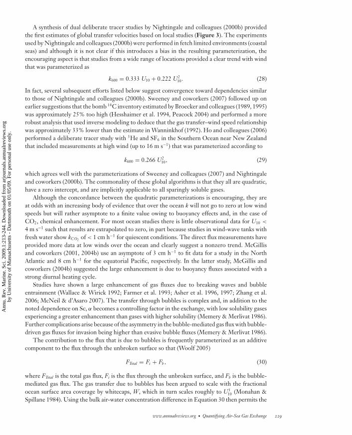
A synthesis of dual deliberate tracer studies by Nightingale and colleagues (2000b) providedthe first estimates of global transfer velocities based on local studies (Figure 3). The experimentsused by Nightingale and colleagues (2000b) were performed in fetch limited environments (coastalseas) and although it is not clear if this introduces a bias in the resulting parameterization, theencouraging aspect is that studies from a wide range of locations provided a clear trend with windthat was parameterized as
k600 = 0.333 U10 + 0.222 U210. (28)
In fact, several subsequent efforts listed below suggest convergence toward dependencies similarto those of Nightingale and colleagues (2000b). Sweeney and coworkers (2007) followed up onearlier suggestions that the bomb 14C inventory estimated by Broecker and colleagues (1989, 1995)was approximately 25% too high (Hesshaimer et al. 1994, Peacock 2004) and performed a morerobust analysis that used inverse modeling to deduce that the gas transfer–wind speed relationshipwas approximately 33% lower than the estimate in Wanninkhof (1992). Ho and colleagues (2006)performed a deliberate tracer study with 3He and SF6 in the Southern Ocean near New Zealandthat included measurements at high wind (up to 16 m s−1) that was parameterized according to
k600 = 0.266 U210, (29)
which agrees well with the parameterizations of Sweeney and colleagues (2007) and Nightingaleand coworkers (2000b). The commonality of these global algorithms is that they all are quadratic,have a zero intercept, and are implicitly applicable to all sparingly soluble gases.
Although the concordance between the quadratic parameterizations is encouraging, they areat odds with an increasing body of evidence that over the ocean k will not go to zero at low windspeeds but will rather asymptote to a finite value owing to buoyancy effects and, in the case ofCO2, chemical enhancement. For most ocean studies there is little observational data for U10 <
4 m s−1 such that results are extrapolated to zero, in part because studies in wind-wave tanks withfresh water show kC O2 of < 1 cm h−1 for quiescent conditions. The direct flux measurements haveprovided more data at low winds over the ocean and clearly suggest a nonzero trend. McGillisand coworkers (2001, 2004b) use an asymptote of 3 cm h−1 to fit data for a study in the NorthAtlantic and 8 cm h−1 for the equatorial Pacific, respectively. In the latter study, McGillis andcoworkers (2004b) suggested the large enhancement is due to buoyancy fluxes associated with astrong diurnal heating cycle.
Studies have shown a large enhancement of gas fluxes due to breaking waves and bubbleentrainment (Wallace & Wirick 1992; Farmer et al. 1993; Asher et al. 1996, 1997; Zhang et al.2006; McNeil & d’Asaro 2007). The transfer through bubbles is complex and, in addition to thenoted dependence on Sc, α becomes a controlling factor in the exchange, with low solubility gasesexperiencing a greater enhancement than gases with higher solubility (Memery & Merlivat 1986).Further complications arise because of the asymmetry in the bubble-mediated gas flux with bubble-driven gas fluxes for invasion being higher than evasive bubble fluxes (Memery & Merlivat 1986).
The contribution to the flux that is due to bubbles is frequently parameterized as an additivecomponent to the flux through the unbroken surface so that (Woolf 2005)
FTotal = Fi + Fb , (30)
where FTotal is the total gas flux, Fi is the flux through the unbroken surface, and Fb is the bubble-mediated gas flux. The gas transfer due to bubbles has been argued to scale with the fractionalocean surface area coverage by whitecaps, W, which in turn scales roughly to U3
10 (Monahan &Spillane 1984). Using the bulk air-water concentration difference in Equation 30 then permits the
www.annualreviews.org • Quantifying Air-Sea Gas Exchange 229
Ann
u. R
ev. M
arin
e. S
ci. 2
009.
1:21
3-24
4. D
ownl
oade
d fr
om a
rjou
rnal
s.an
nual
revi
ews.
org
by U
nive
rsity
of
Mas
sach
uset
ts -
Dar
tmou
th o
n 01
/05/
09. F
or p
erso
nal u
se o
nly.

ANRV396-MA01-10 ARI 4 November 2008 8:3
net transfer velocity k to be expressed as an area weighted average given by
k = ki (1 − W ) + kb W, (31)
where ki is the transfer velocity through the unbroken surface and kb is the bubble-mediatedtransfer velocity. Although modeling studies (Memery & Merlivat 1986, Woolf & Thorpe 1991,Woolf 2005) and laboratory measurements (Asher et al. 1996, 1997; Komori & Misumi 2002;Woolf et al. 2007) have attempted to determine a function form for kb in terms of physicochemicalvariables, its precise definition remains elusive.
Despite the fact that the details of kb are unknown, it is possible to study the dependence ofk on breaking waves using the available field data. Using the GasEx-98 dataset, McGillis andcoworkers (2001) assumed that the observed increase in k with U10 was controlled by breakingwaves and that ki was constant with U10. These assumptions lead to a functional form for kgiven by k = a + b U3
10, assuming W � 1. This is a reasonable assumption because W ≈ 0.02 forU10 ≈ 20 m s−1 (for instance, Asher et al. 2002). Using this functional form, McGillis and coworkers(2001) found that for the GasEx-98 data, k could be parameterized by:
k660 = 3.3 + 0.026 U310, (32)
with a similar result for the data from the GasEx-2001 experiment (McGillis et al. 2004b):
k660 = 8.2 + 0.014 U310. (33)
The relationships, along with the binned data, are shown in Figure 4. Using a similar approachas that used with the GasEx-98 dataset, Asher and coworkers (2002) found excellent agreementbetween the oceanic k values and those predicted from a whitecap-based model via the use of anempirically derived functional form for kb and measured values for W. However, a caution mustbe placed on assuming Equations 32, 33, or the parameterization given by Asher and cowork-ers (2002) represent a general relation for whitecap-driven gas transfer. Because the GasEx-98dataset is for CO2 invasion and the GasEx-2001 dataset is for evasion, and because a known asym-metry exists between invasion and evasion when bubble-mediated processes are important, therelations discussed here apply only to these specific cases. Overall, although it is understood thatwhitecaps play an important role in air-sea gas transfer, especially at high wind speeds, accurateparameterization of this effect remains elusive.
Issues in The Use of Gas Exchange–Wind Speed Relationships
When using gas exchange–wind speed relationships to calculate regional or global-scale fluxes,it is important to use consistent winds. Global mean wind speed estimates can differ by morethan 1 m s−1 (Boutin et al. 2002, Naegler et al. 2006). For instance, the NCEP assimilatedproduct yields a global average wind of 6.6 m s−1 and the global average QuikSCAT satel-lite winds are 7.9 m s−1 (Naegler et al. 2006), which will result in biases in global CO2 fluxesof (7.9/6.6)2 or 43% for quadratic dependencies and (7.9/6.6)3 or 71% for cubic relationships(Wanninkhof et al. 2002). Spatial distributions of winds are not consistent among different windspeed climatologies either. In particular, the mean U10 in the equatorial Pacific region can dif-fer by as much as 2 m s−1 depending on which climatological wind speed is used. C. Sweeney(unpublished data) demonstrates with a numerical model that although the bomb 14C constraintyields consistent global mean gas transfer velocities for different wind speed climatologies, therelative difference in wind speeds in the Equatorial and Southern oceans yields a difference inglobal mean air-sea CO2 flux of 0.5 Pg year−1 (or ∼25%) using a quadratic dependence betweenk and U10.
230 Wanninkhof et al.
Ann
u. R
ev. M
arin
e. S
ci. 2
009.
1:21
3-24
4. D
ownl
oade
d fr
om a
rjou
rnal
s.an
nual
revi
ews.
org
by U
nive
rsity
of
Mas
sach
uset
ts -
Dar
tmou
th o
n 01
/05/
09. F
or p
erso
nal u
se o
nly.
ANRV396-MA01-10 ARI 4 November 2008 8:3
0 5 10 15 20
10 (m s–1)
66
0 (
cm h
–1)
0
20
40
60
80
100
120
N.Atl GasEx-98Eq. Pac. GasEx-01
Equation 32Equation 33
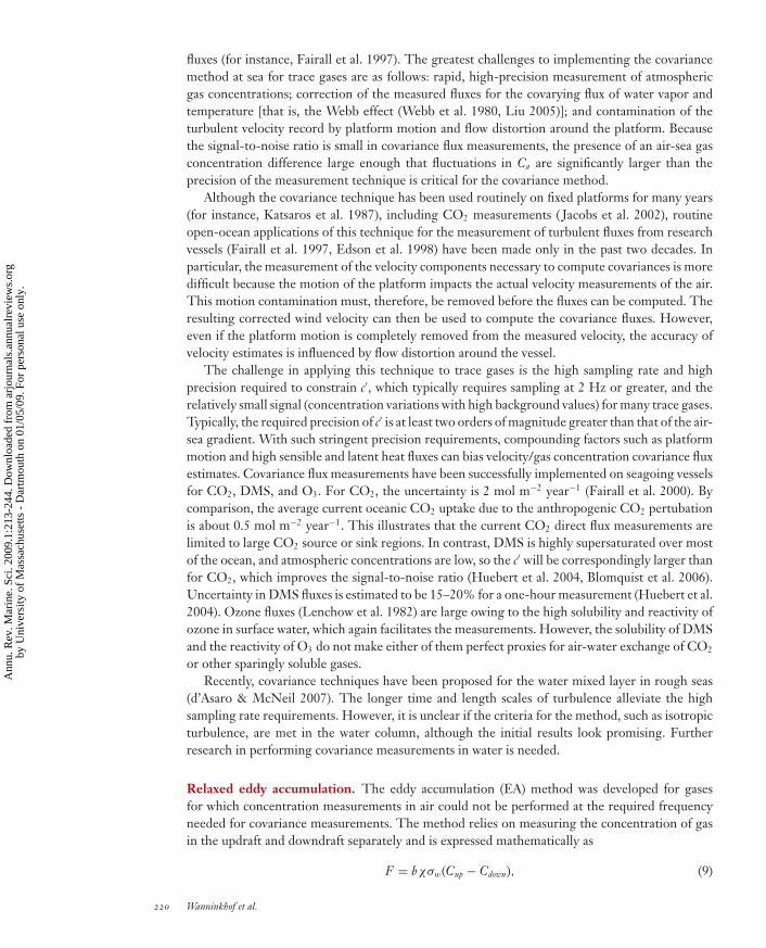
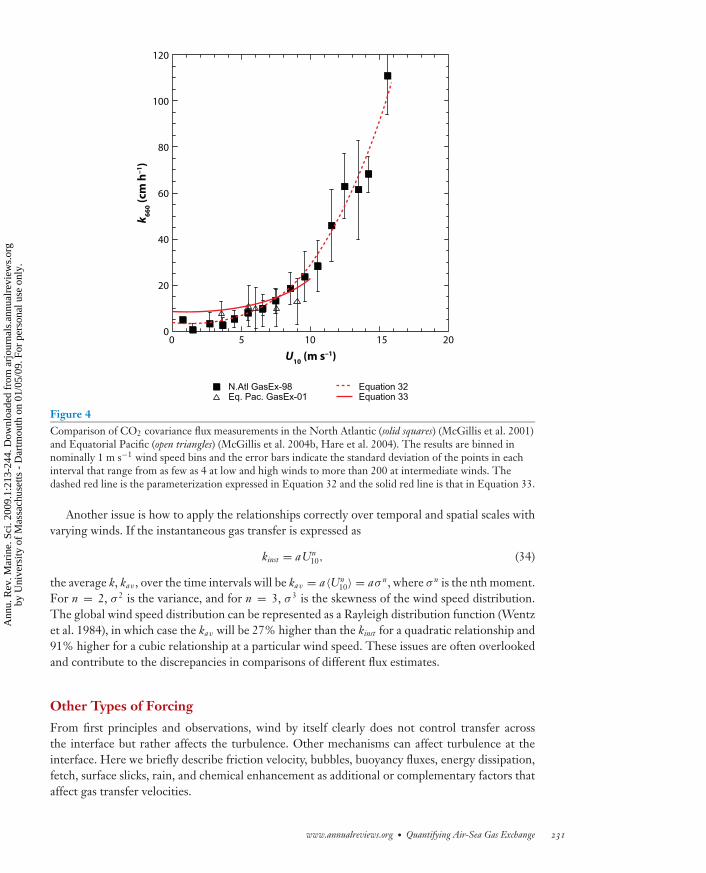
Figure 4Comparison of CO2 covariance flux measurements in the North Atlantic (solid squares) (McGillis et al. 2001)and Equatorial Pacific (open triangles) (McGillis et al. 2004b, Hare et al. 2004). The results are binned innominally 1 m s−1 wind speed bins and the error bars indicate the standard deviation of the points in eachinterval that range from as few as 4 at low and high winds to more than 200 at intermediate winds. Thedashed red line is the parameterization expressed in Equation 32 and the solid red line is that in Equation 33.
Another issue is how to apply the relationships correctly over temporal and spatial scales withvarying winds. If the instantaneous gas transfer is expressed as
kinst = aUn10, (34)
the average k, kav , over the time intervals will be kav = a〈Un10〉 = aσ n, where σ n is the nth moment.
For n = 2, σ 2 is the variance, and for n = 3, σ 3 is the skewness of the wind speed distribution.The global wind speed distribution can be represented as a Rayleigh distribution function (Wentzet al. 1984), in which case the kav will be 27% higher than the kinst for a quadratic relationship and91% higher for a cubic relationship at a particular wind speed. These issues are often overlookedand contribute to the discrepancies in comparisons of different flux estimates.
Other Types of Forcing
From first principles and observations, wind by itself clearly does not control transfer acrossthe interface but rather affects the turbulence. Other mechanisms can affect turbulence at theinterface. Here we briefly describe friction velocity, bubbles, buoyancy fluxes, energy dissipation,fetch, surface slicks, rain, and chemical enhancement as additional or complementary factors thataffect gas transfer velocities.
www.annualreviews.org • Quantifying Air-Sea Gas Exchange 231
Ann
u. R
ev. M
arin
e. S
ci. 2
009.
1:21
3-24
4. D
ownl
oade
d fr
om a
rjou
rnal
s.an
nual
revi
ews.
org
by U
nive
rsity
of
Mas
sach
uset
ts -
Dar
tmou
th o
n 01
/05/
09. F
or p
erso
nal u
se o
nly.

ANRV396-MA01-10 ARI 4 November 2008 8:3
Friction velocity is a better environmental variable to estimate gas transfer than wind becauseit is intrinsically related to turbulence at the water surface. Several of the first-order parameteri-zations (see Equations 21 and 22) are expressed in terms of friction velocity. Large & Pond (1981)provide a full description of the relationship between U10 and ua∗ for different environmentalconditions. For low winds and neutral stability, they determined that Cd is invariant, whereas atintermediate winds Cd scales linearly with wind speed. The relationship between U10 and ua∗ willvary depending on wave state and surfactant concentrations. Erickson (1993) derived relationshipsthat incorporate boundary layer stability as it affects ua∗ into his parameterizations.
At low winds, it is not only ua∗ , but also buoyancy fluxes that will affect surface turbulence.Buoyancy fluxes are not readily parameterized without a full knowledge of heat and momentumfluxes but can be included in parameterizations as outlined by Fairall et al. (2000) (see Equation22). On the basis of direct flux measurements of CO2 in the equatorial Pacific, these effects canbe significant in areas with high heat fluxes (McGillis et al. 2004b).
An alternative perspective suggests that gas exchange is controlled by the dissipation of energyat the surface rather than stress or ua∗ . Several controlled studies provide support for this concept(Asher & Pankow 1986, Zappa et al. 2007). The practical implication of this suggestion is thatthe dissipation scales roughly to the cube of the wind, which lends support for strongly nonlineardependencies of k on U10.
Irrespective of the mechanism of gas transfer, it is clear that wave field will strongly affectthe exchange. Therefore, fetch, the distance the winds blow over the ocean, is believed to have afirst-order effect on the transfer. Results of field studies using eddy correlation techniques showa fetch effect for ozone (Fairall et al. 2006). Theoretical work by Woolf (2005) suggests that theeffect is significant for fetches up to 1000 km in large part because of development of breakingwave fields and contributions by bubbles to gas transfer.
Bubble effects are often considered additive to transfer across the air-water interface (see Equa-tions 30 and 31). Bubbles can greatly enhance the exchange of gases across the air-sea interface byextreme turbulence associated with wave breaking and the rise of the plume back to the surface,and by transfer of gases through the walls of individual bubbles. In the latter case, the solubility ofthe gas becomes an important factor; lower solubility gases experience a greater bubble enhance-ment than gases with greater solubility. Studies suggest that the enhancement by bubbles can bescaled roughly to the cube of the wind with a strong solubility dependence (Asher et al. 2002).Woolf (1997) estimated that bubbles contribute 30% of the global gas transfer velocity of CO2.The exact magnitude of the effect of bubbles on gas transfer, and CO2 fluxes in particular, remainsan active resesearch area but there is general consensus that bubbles play a first order role in gastransfer.
Surfactants inhibit the exchange primarily through inhibition of surface turbulence (Frew1997). Wind-wave tank results show that surfactants at very low concentrations retard gas transferat the highest wind speeds studied, suggesting that gas exchange in the ocean is for practicalpurposes always affected by naturally occurring surfactants. Surfactants decrease the gas exchangeand also uw∗ under a smooth surface regime such that decreases in k scale with decreases in uw∗ .The decreases in k at higher winds/turbulent conditions are more difficult to quantify with forcing.The retardation of the net air-sea CO2 flux over the ocean due to surfactants is estimated to beas large as 20% to 50% based on the laboratory results and remotely sensed data of the effectsof surfactants on waves, and estimates of surfactant concentrations due to biological productivity(Tsai & Liu 2003). However, Asher (1997) concluded that surfactants would actually increasethe net CO2 flux because the effects are most pronounced in regions with low winds where thedirection of CO2 flux is out of the ocean (Figure 5). The widely divergent results indicate theuncertainty of the surfactant effect on gas transfer and CO2 fluxes over the ocean.
232 Wanninkhof et al.
Ann
u. R
ev. M
arin
e. S
ci. 2
009.
1:21
3-24
4. D
ownl
oade
d fr
om a
rjou
rnal
s.an
nual
revi
ews.
org
by U
nive
rsity
of
Mas
sach
uset
ts -
Dar
tmou
th o
n 01
/05/
09. F
or p
erso
nal u
se o
nly.
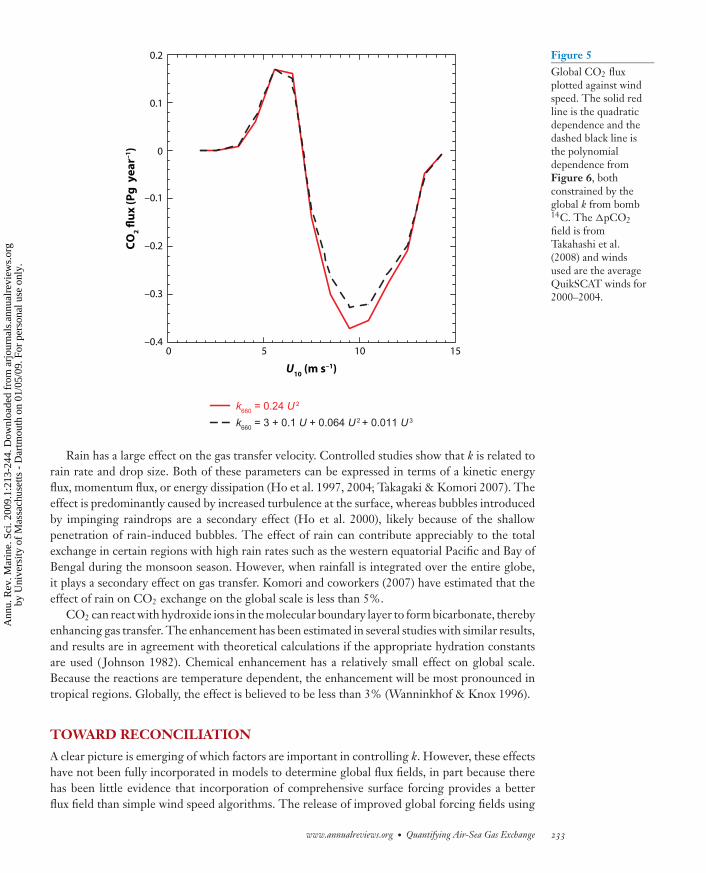
ANRV396-MA01-10 ARI 4 November 2008 8:3
–0.4
–0.3
0 5 10 15
–0.2
–0.1
0
0.1
0.2
10 (m s–1)
CO
2 fl
ux
(P
g y
ea
r–1)
k660
= 0.24 U 2
k660
= 3 + 0.1 U + 0.064 U 2 + 0.011 U 3
Figure 5Global CO2 fluxplotted against windspeed. The solid redline is the quadraticdependence and thedashed black line isthe polynomialdependence fromFigure 6, bothconstrained by theglobal k from bomb14C. The �pCO2field is fromTakahashi et al.(2008) and windsused are the averageQuikSCAT winds for2000–2004.
Rain has a large effect on the gas transfer velocity. Controlled studies show that k is related torain rate and drop size. Both of these parameters can be expressed in terms of a kinetic energyflux, momentum flux, or energy dissipation (Ho et al. 1997, 2004; Takagaki & Komori 2007). Theeffect is predominantly caused by increased turbulence at the surface, whereas bubbles introducedby impinging raindrops are a secondary effect (Ho et al. 2000), likely because of the shallowpenetration of rain-induced bubbles. The effect of rain can contribute appreciably to the totalexchange in certain regions with high rain rates such as the western equatorial Pacific and Bay ofBengal during the monsoon season. However, when rainfall is integrated over the entire globe,it plays a secondary effect on gas transfer. Komori and coworkers (2007) have estimated that theeffect of rain on CO2 exchange on the global scale is less than 5%.
CO2 can react with hydroxide ions in the molecular boundary layer to form bicarbonate, therebyenhancing gas transfer. The enhancement has been estimated in several studies with similar results,and results are in agreement with theoretical calculations if the appropriate hydration constantsare used ( Johnson 1982). Chemical enhancement has a relatively small effect on global scale.Because the reactions are temperature dependent, the enhancement will be most pronounced intropical regions. Globally, the effect is believed to be less than 3% (Wanninkhof & Knox 1996).
TOWARD RECONCILIATION
A clear picture is emerging of which factors are important in controlling k. However, these effectshave not been fully incorporated in models to determine global flux fields, in part because therehas been little evidence that incorporation of comprehensive surface forcing provides a betterflux field than simple wind speed algorithms. The release of improved global forcing fields using
www.annualreviews.org • Quantifying Air-Sea Gas Exchange 233
Ann
u. R
ev. M
arin
e. S
ci. 2
009.
1:21
3-24
4. D
ownl
oade
d fr
om a
rjou
rnal
s.an
nual
revi
ews.
org
by U
nive
rsity
of
Mas
sach
uset
ts -
Dar
tmou
th o
n 01
/05/
09. F
or p
erso
nal u
se o
nly.
ANRV396-MA01-10 ARI 4 November 2008 8:3
remote sensing offers an opportunity to make meaningful advances. Algorithms can be establishedthat utilize the direct returns from remotely sensed products, or products derived from remotesensing, data assimilation, and/or modeling can be used.
Surface water concentration climatologies of several gases are currently available (for instance,for DMS, Kettle & Andreae 2000). However, these climatologies lack comprehensive data coverageand often rely on bold temporal and spatial extrapolations. The most comprehensive observation-based global climatology of pCO2 is that of Takahashi and colleagues (2008). The surface waterpCO2 fields are derived from approximately three million surface water observations used incombination with a surface flow field from a general circulation model to determine pCO2 on a4◦ by 5◦ grid with monthly resolution. Mole fractions of CO2 in air are obtained from a well-constrained interpolated global dataset (Coop. Atmos. Data Integr. Proj. 2007), which, combinedwith ambient pressure, yields the pCO2 in air. The k is determined from wind speed assuminga quadratic dependence that is scaled to the revised global bomb 14C constraint (Sweeney et al.2007). The derived global net flux into the ocean of 1.6 Pg C year−1 is in good agreement withthe global estimate of anthropogenic CO2 uptake obtained from independent mass balance andisotopic methods of 2.2 Pg C year−1 when accounting for a riverine flux of 0.4 Pg C year−1 andfor the fact that the climatology is for a non–El Nino year. The inclusion of El Nino years isthought to contribute on average an additional 0.2 Pg C year−1 to the flux estimate, yielding atotal anthropogenic flux ( = net flux + riverine input + El Nino contribution) of 2 Pg C year−1 bythis method. The uncertainty is estimated at 0.7 Pg C year−1 with approximately 30% attributedto the uncertainty in the coefficient between k and U2
10 and 20% attributed to uncertainty in thewinds. However, these rough uncertainty estimates do not necessarily account for regional biasesand compensating errors. Advances in quantifying the forcing of gas exchange on global scalesoffers an opportunity to provide more robust estimates of k.
To create a global flux product, variability in both the concentration fields and forcing mustbe accounted for at grid scales at least as small as the concentration field grid. Wind speed hasbeen the forcing field of choice because of its availability on a global scale for many applications,including ocean modeling. It is not clear, however, that wind speed is actually the best represen-tation of surface turbulence. The near-synoptic coverage offered through satellite remote sensingprovides attractive opportunities to determine forcing, not only because it is at the appropriateresolution, but also because satellite observations of the sea surface wave slope may be a betterdirect measurement of turbulence than wind speed. The wave slope is determined from satellitesensors using specific wavebands that represent surface roughness at 10–30-cm scales. Glover andcoworkers (2002) took advantage of the strong correlation between wave slope and k along withwave slope information from altimeters to estimate global k at high resolution. Altimeters providegood information on waves but have global coverage on a 10-day repeat cycle, thereby missingtemporal variability (Frew et al. 2007). Scatterometers provide significantly better coverage, butobtaining meaningful wave slope information from their wide swath is challenging. The globalk fields obtained in this fashion appear to underestimate the k at high winds, likely because theeffect of bubbles is not implicitly included in their algorithms. Refinements of the approach areunderway but it is not clear if the fidelity of the k versus wave slope algorithms derived fromaltimetry and/or scatterometry is superior to the relationships with wind speed derived from thesame sensors.
Another approach is to use a model that incorporates the processes known to affect the gastransfer, taking advantage of the global surface fields of wind stress, heat, and momentum suchas provided by the National Centers for Environmental Prediction (NCEP). The derivation byFairall and coworkers (2000) (Equation 22) offers good opportunities in this respect, in particularwhen the effects of bubbles and chemical enhancement are included as extra terms. The scalable
234 Wanninkhof et al.
Ann
u. R
ev. M
arin
e. S
ci. 2
009.
1:21
3-24
4. D
ownl
oade
d fr
om a
rjou
rnal
s.an
nual
revi
ews.
org
by U
nive
rsity
of
Mas
sach
uset
ts -
Dar
tmou
th o
n 01
/05/
09. F
or p
erso
nal u
se o
nly.
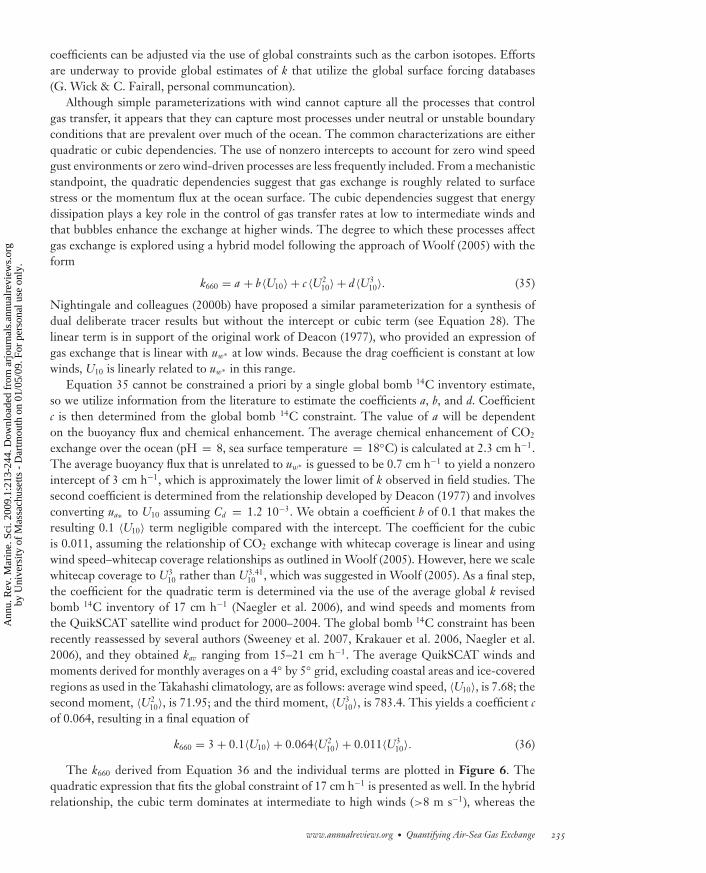
ANRV396-MA01-10 ARI 4 November 2008 8:3
coefficients can be adjusted via the use of global constraints such as the carbon isotopes. Effortsare underway to provide global estimates of k that utilize the global surface forcing databases(G. Wick & C. Fairall, personal communcation).
Although simple parameterizations with wind cannot capture all the processes that controlgas transfer, it appears that they can capture most processes under neutral or unstable boundaryconditions that are prevalent over much of the ocean. The common characterizations are eitherquadratic or cubic dependencies. The use of nonzero intercepts to account for zero wind speedgust environments or zero wind-driven processes are less frequently included. From a mechanisticstandpoint, the quadratic dependencies suggest that gas exchange is roughly related to surfacestress or the momentum flux at the ocean surface. The cubic dependencies suggest that energydissipation plays a key role in the control of gas transfer rates at low to intermediate winds andthat bubbles enhance the exchange at higher winds. The degree to which these processes affectgas exchange is explored using a hybrid model following the approach of Woolf (2005) with theform
k660 = a + b〈U10〉 + c 〈U210〉 + d 〈U3
10〉. (35)
Nightingale and colleagues (2000b) have proposed a similar parameterization for a synthesis ofdual deliberate tracer results but without the intercept or cubic term (see Equation 28). Thelinear term is in support of the original work of Deacon (1977), who provided an expression ofgas exchange that is linear with uw∗ at low winds. Because the drag coefficient is constant at lowwinds, U10 is linearly related to uw∗ in this range.
Equation 35 cannot be constrained a priori by a single global bomb 14C inventory estimate,so we utilize information from the literature to estimate the coefficients a, b, and d. Coefficientc is then determined from the global bomb 14C constraint. The value of a will be dependenton the buoyancy flux and chemical enhancement. The average chemical enhancement of CO2
exchange over the ocean (pH = 8, sea surface temperature = 18◦C) is calculated at 2.3 cm h−1.The average buoyancy flux that is unrelated to uw∗ is guessed to be 0.7 cm h−1 to yield a nonzerointercept of 3 cm h−1, which is approximately the lower limit of k observed in field studies. Thesecond coefficient is determined from the relationship developed by Deacon (1977) and involvesconverting ua∗ to U10 assuming Cd = 1.2 10−3. We obtain a coefficient b of 0.1 that makes theresulting 0.1 〈U10〉 term negligible compared with the intercept. The coefficient for the cubicis 0.011, assuming the relationship of CO2 exchange with whitecap coverage is linear and usingwind speed–whitecap coverage relationships as outlined in Woolf (2005). However, here we scalewhitecap coverage to U3
10 rather than U3.4110 , which was suggested in Woolf (2005). As a final step,
the coefficient for the quadratic term is determined via the use of the average global k revisedbomb 14C inventory of 17 cm h−1 (Naegler et al. 2006), and wind speeds and moments fromthe QuikSCAT satellite wind product for 2000–2004. The global bomb 14C constraint has beenrecently reassessed by several authors (Sweeney et al. 2007, Krakauer et al. 2006, Naegler et al.2006), and they obtained kav ranging from 15–21 cm h−1. The average QuikSCAT winds andmoments derived for monthly averages on a 4◦ by 5◦ grid, excluding coastal areas and ice-coveredregions as used in the Takahashi climatology, are as follows: average wind speed, 〈U10〉, is 7.68; thesecond moment, 〈U2
10〉, is 71.95; and the third moment, 〈U310〉, is 783.4. This yields a coefficient c
of 0.064, resulting in a final equation of
k660 = 3 + 0.1〈U10〉 + 0.064〈U210〉 + 0.011〈U3
10〉. (36)
The k660 derived from Equation 36 and the individual terms are plotted in Figure 6. Thequadratic expression that fits the global constraint of 17 cm h−1 is presented as well. In the hybridrelationship, the cubic term dominates at intermediate to high winds (>8 m s−1), whereas the
www.annualreviews.org • Quantifying Air-Sea Gas Exchange 235
Ann
u. R
ev. M
arin
e. S
ci. 2
009.
1:21
3-24
4. D
ownl
oade
d fr
om a
rjou
rnal
s.an
nual
revi
ews.
org
by U
nive
rsity
of
Mas
sach
uset
ts -
Dar
tmou
th o
n 01
/05/
09. F
or p
erso
nal u
se o
nly.

ANRV396-MA01-10 ARI 4 November 2008 8:3
0 5 10 15 20
10 (m s–1)
66
0 (
cm h
–1)
0
20
40
60
80
100
30.1*U
10
3 + 0.1 U10
+ 0.064 U10
2 + 0.011 U10
3
Global k (Naegler et al. 2006) 0.064 U
102
0.011 U10
3
0.236 U10
2
Figure 6Comparison of the polynomial function with wind (Equation 36) (blue line) with a quadratic (Equation 37)(red line), all constrained by the average k from bomb 14C (Naegler et al. 2006). The dashed lines are theindividual terms in Equation 36 listed in the legend.
constant term dominates at winds of less than 3 m s−1. However, a quadratic fit that meets theglobal constraint is nearly indistinguishable from the hybrid form for winds <15 m s−1,
k660 = 0.24〈U210〉. (37)
Considering that for a global Rayleigh wind distribution 96% of the winds are below 15 m s−1,a simple quadratic dependence appears, at first glance, adequate for an empirical relationship(Figure 6).
To determine the difference between the polynomial expression and a quadratic function inglobal CO2 flux estimates, we apply the parameterizations of Equations 36 and 37 to the CO2
climatology of Takahashi and coworkers (2008). Equation 37 yields an uptake of –1.3 Pg C year−1,
whereas the polynomial expression (Equation 36) gives a net uptake of –1.14 Pg C year−1, or a 15%difference. The distribution of fluxes is plotted against monthly mean wind speed in Figure 5.The slightly lower dependence of Equation 36 compared with Equation 37 at winds between 6
236 Wanninkhof et al.
Ann
u. R
ev. M
arin
e. S
ci. 2
009.
1:21
3-24
4. D
ownl
oade
d fr
om a
rjou
rnal
s.an
nual
revi
ews.
org
by U
nive
rsity
of
Mas
sach
uset
ts -
Dar
tmou
th o
n 01
/05/
09. F
or p
erso
nal u
se o
nly.

ANRV396-MA01-10 ARI 4 November 2008 8:3
and 12 m s−1 leads to a lower CO2 flux into the ocean. This result emphasizes the need for accurateparameterizations.
The effect of different wind speed relationships on global CO2 fluxes is as follows: For the samefunctional dependencies, the global CO2 flux will scale proportionally with the coefficients if thesame wind speed product is used. Different functional dependencies, even if they are scaled to thesame global mean k fluxes, can yield significantly different CO2 fluxes. Higher-order dependen-cies generally exhibit lower global CO2 uptake because they yield lower k at intermediate winds(≈6–10 m s−1) that are prevalent over the ocean and because most of the flux into the ocean iswithin these wind speed ranges (Figure 5).
SUMMARY POINTS
1. The application of direct flux meteorological techniques to measure gas fluxes makes itpossible to measure fluxes at the same time and space scales as the environmental forcingprocesses.
2. Micrometeorological approaches have put the gas transfer on a sound theoretical foun-dation through invoking similarity with heat and momentum fluxes.
3. Infrared imaging techniques have improved the understanding and quantification ofnear-surface turbulence on small scales.
4. Satellite remote sensing and data assimilation provide comprehensive global fields ofenvironmental forcing, including wind, sea surface temperature, air temperature, andfriction velocity.
5. Dual deliberate tracer studies provide a means to quantify k at any desired locale withtimescales on the order of a day.
6. A wind speed–only polynomial function is developed to determine the gas transfer veloc-ity that can be well approximated by a conventional quadratic function for the prevalentwind speed range. However, the small difference in functionality at intermediate windshas an appreciable effect on the calculated global CO2 fluxes.
7. The role of breaking waves at high wind speeds is recognized as important, but as yetthere remains no reliable way to accurately quantify the effect of breaking waves on gasexchange.
DISCLOSURE STATEMENT
The authors are not aware of any biases that might be perceived as affecting the objectivity of thisreview.
ACKNOWLEDGMENTS
Discussions with participants of the K-Conundrum Workshop sponsored by the Surface Ocean-Lower Atmosphere Study (SOLAS) and the European Union COST Program in Norwich, UnitedKingdom in February 2008 were very beneficial in producing this work. We appreciate the expertcopyediting and proofreading by Gail Derr of NOAA/AOML.
www.annualreviews.org • Quantifying Air-Sea Gas Exchange 237
Ann
u. R
ev. M
arin
e. S
ci. 2
009.
1:21
3-24
4. D
ownl
oade
d fr
om a
rjou
rnal
s.an
nual
revi
ews.
org
by U
nive
rsity
of
Mas
sach
uset
ts -
Dar
tmou
th o
n 01
/05/
09. F
or p
erso
nal u
se o
nly.

ANRV396-MA01-10 ARI 4 November 2008 8:3
Appendix A
List of Symbolsα Ostwald solubility coefficient (nondimensional) Fi Flux through the unbroken surfaceδ Thickness of the stagnant film h Water depth that is in contact with air; defined as V/A
(mixed layer depth)ε Chemical enhancement factor I Deficit of 222Rn relative to 226Ra in the mixed layerεc Turbulent kinetic energy dissipation k Gas transfer velocityεkw Gas transfer velocities of the gas through the
diffusive sublayer layers on the water sidek660 Gas transfer velocity normalized to a Sc number of 660
ka/α Gas transfer velocities of the gas through thediffusive sublayer on the air side
kav Average gas transfer velocity
� Adjustable parameter kb Bubble-mediated transfer velocityν Kinematic viscosity of water ki Transfer velocity through the unbroken surfaceσw Standard deviation of vertical velocity kinst Instantaneous gas transfer velocityϕ Empirical function that accounts for buoyancy
effects on turbulent transferKo Aqueous-phase solubility
λ Radioactive decay constant L Turbulence integral length scaleκ Von Karman constant (≈0.4) M Mass of gas in waterρa Density of air pCO2a Partial pressure of CO2 in airρw Density of water pCO2w Partial pressure of CO2 in waterσ n (Statistical) nth moment Q Velocity scale222Rn Isotope of radon R Ideal gas constant226Ra Isotope of radium R1,2 Transfer resistance between the heights of
measurement in air3He Light isotope of helium Rair Air-side resistance to gas transfera Constant Rr Roughness Reynolds numberA Radioactive activity Rwater Water-side resistance to gas transferA Surface area S Sources or sinks other than the air-sea fluxbχ Parameter that depends on the threshold and
characteristic length scales of turbulenceSc Schmidt number (nondimensional)
c′ Fluctuations of gas concentration about a mean SF6 Sulfur hexafluorideCd Drag coefficient TW Water temperatureCa Concentration of the gas in the air U Wind speedCo Gas concentration at the water surface u∗ Water-side friction velocityCw Gas concentration in the well-mixed bulk fluid
below the surfaceU10 Wind speed at 10-m height under neutral boundary
conditionsCz1 Concentration at height z1 in the atmospheric
boundary layerua∗ Friction velocity in air
D Molecular diffusivity uw∗ Surface friction velocity in waterF Air-sea gas flux V Water volumeFb Bubble-mediated gas flux W Fractional white cap coverage
w Vertical velocity
238 Wanninkhof et al.
Ann
u. R
ev. M
arin
e. S
ci. 2
009.
1:21
3-24
4. D
ownl
oade
d fr
om a
rjou
rnal
s.an
nual
revi
ews.
org
by U
nive
rsity
of
Mas
sach
uset
ts -
Dar
tmou
th o
n 01
/05/
09. F
or p
erso
nal u
se o
nly.

ANRV396-MA01-10 ARI 4 November 2008 8:3
LITERATURE CITED
Asher WE. 1997. The sea surface microlayer and its effect on global air-sea gas transfer. See Liss & Duce1997, pp. 251–86
Asher WE, Edson JB, McGillis WR, Wanninkhof R, Ho DT, Litchendorf T. 2002. Fractional area white-cap coverage and air-sea gas transfer velocities measured during GasEx-98. See Donelan et al. 2002,pp. 199–204
Asher WE, Farley PJ, Higgins BJ, Karle LM, Monahan EC, Leifer IS. 1996. The influence of bubble plumeson air/seawater gas transfer velocities. J. Geophys. Res. 101:12027–41
Asher WE, Jessup AT, Atmane MA. 2004. Oceanic application of the active controlled flux technique formeasuring air-sea transfer velocities of heat and gases. J. Geophys. Res. 109:C08S12
Asher WE, Karle LM, Higgins BJ. 1997. On the differences between bubble-mediated air-water gas transferin freshwater and seawater. J. Mar. Res. 55:813–45
Asher WE, Pankow JF. 1986. The interaction of mechanically generated turbulence and interfacial films witha liquid phase controlled gas/liquid transport process. Tellus B 38:305–18
Asher WE, Pankow JF. 1989. Direct observation of concentration fluctuations close to a gas/liquid interface.Chem. Eng. Sci. 44:1451–55
Asher WE, Wanninkhof R. 1998. Transient tracers and air-sea gas transfer. J. Geophys. Res. 103:15939–58Atmane MA, Asher WE, Jessup AT. 2004. On the use of the active infrared technique to infer heat and gas
transfer velocities at the air-water free surface. J. Geophys. Res. 109:C08S14Banerjee S, Lakehal D, Fulgosi M. 2004. Surface divergence models for scalar exchange between turbulent
streams. Int. J. Multiph. Flow 30:963–73Blomquist BW, Fairall CW, Huebert BJ, Kieber DJ, Westby GR. 2006. DMS sea-air transfer velocity: direct
measurements by eddy covariance and parameterization based on the NOAA/COARE gas transfer model.Geophys. Res. Lett. 32:L07601
Bock EJ, Hara T, Frew NM, McGillis WR. 1999. Relationship between air-sea gas transfer and short windwaves. J. Geophys. Res. 104:25821–32
Borges AV, Wanninkhof R. 2007. Preface: 37th International Liege Colloquium on Ocean Dynamics, Liege,Belgium, May 2–6, 2005, 5th International Symposium on Gas Transfer at Water Surfaces. J. Mar. Sys.66:1–3
Boutin J, Etcheto J, Merlivat L, Rangama Y. 2002. Influence of gas exchange coefficient parameterisation onseasonal and regional variability of CO2 air-sea fluxes. Geophys. Res. Lett. 29(8):1182
Broecker HC, Peterman J, Siems W. 1978. The influence of wind on CO2 exchange in a wind wave tunnel,including the effects of monolayers. J. Mar. Res. 36:595–610
Broecker WS, Ledwell JR, Takahashi T, Weiss R, Merlivat L, et al. 1986. Isotopic versus micrometeorologicocean CO2 fluxes: A serious conflict. J. Geophys. Res. 91(C9):10517–27
Broecker WS, Peng T-H, Ostlund G, Stuiver M. 1985. The distribution of bomb radiocarbon in the ocean.J. Geophys. Res. 99:6953–70
Broecker WS, Sutherland S, Smethie W, Peng T-H, Ostlund G. 1995. Oceanic radiocarbon: separation ofthe natural and bomb components. Glob. Biogeochem. Cycles 9:263–88
Brumley BH, Jirka GH. 1988. Air-water transfer of slightly soluble gases: turbulence, interfacial processes andconceptual models. Phys. Chem. Hydrodyn. 10:295–319
Brutsaert W, Jirka GH, ed. 1984. Gas Transfer at Water Surfaces. Hingham, MA: Reidel. 639 pp.Businger JA, Delaney AC. 1990. Chemical sensor resolution required for measuring surface fluxes by three
common micrometeorological techniques. J. Atmos. Chem. 19:399–410Cember R. 1989. Bomb radiocarbon in the Red Sea: a medium-scale gas exchange experiment. J. Geophys. Res.
94:2111–23Chang WN, Heikes BG, Lee MH. 2004. Ozone deposition to the sea surface: chemical enhancement and
wind speed dependence. Atmos. Env. 38:1053–59Cooperative Atmospheric Data Integration Project—Carbon Dioxide. 2007. GlobalView-CO2. Boulder, CO:
NOAA ESRL. CD-ROM (also available on Internet via anonymous FTP to ftp.cmdl.noaa.gov, path:ccg/co2/GLOBALVIEW)
www.annualreviews.org • Quantifying Air-Sea Gas Exchange 239
Ann
u. R
ev. M
arin
e. S
ci. 2
009.
1:21
3-24
4. D
ownl
oade
d fr
om a
rjou
rnal
s.an
nual
revi
ews.
org
by U
nive
rsity
of
Mas
sach
uset
ts -
Dar
tmou
th o
n 01
/05/
09. F
or p
erso
nal u
se o
nly.

ANRV396-MA01-10 ARI 4 November 2008 8:3
Craig PD, Banner ML. 1994. Modeling wave-enhanced turbulence in the ocean surface layer. J. Phys. Oceanogr.24:2546–59
d’Asaro ED, McNeil C. 2007. Air-sea gas exchange at extreme winds speeds measured by autonomous oceano-graphic floats. J. Mar. Res. 66:92–109
Danckwerts PV. 1951. Significance of liquid film coefficients in gas absorption. Ind. Eng. Chem. 43:1460–67Danckwerts PV. 1970. Gas-Liquid Reactions. New York: McGraw HillDavies JT. 1972. Turbulence Phenomena: An Introduction to the Eddy Transfer of Momentum, Mass, and Heat,
Particularly at Interfaces. New York: AcademicDavies JT, Kilner AA, Ratcliff GA. 1964. The effect of diffusivities and surface films on rates of gas absorption.
Chem. Eng. Sci. 19:583–90Deacon EL. 1977. Gas transfer to and across an air-water interface. Tellus 29:363–74Donelan MA, Drennan WM, Saltzman ES, Wanninkhof R, ed. 2002. Gas Transfer at Water Surfaces.
Washington, DC: Am. Geophys. Union, Geophys. Monogr. 127. 383 pp.Edson JB, Fairall CW. 1998. Similarity relationships in the marine atmospheric surface layer for terms in the
TKE and scalar variance budgets. J. Atmos. Sci. 55:2311–28Edson JB, Hinton AA, Prada KE, Hare JE, Fairall CW. 1998. Direct covariance flux estimates from mobile
platforms at sea. J. Atmos. Ocean. Technol. 15:547–62Edson JB, Zappa CJ, Ware JA, McGillis WR, Hare JE. 2004. Scalar flux profile relationships over the open
ocean. J. Geophys. Res. 109:C08S09Erickson DJ III. 1993. A stability-dependent theory for air-sea gas exchange. J. Geophys. Res. 98:8471–88Fairall CW, Bariteau L, Grachev AA, Hill RJ, Wolfe DE, et al. 2006. Turbulent bulk transfer coefficients and
ozone deposition velocity in the International Consortium for Atmospheric Research into Transport andTransformation. J. Geophys. Res. 111:D23S20
Fairall CW, Hare JE, Edson JB, McGillis W. 2000. Parameterization and micrometeorological measurementof air-sea gas transfer. Bound. Layer Meteor. 96:63–105
Fairall CW, Larsen SE. 1986. Inertial-dissipation methods and turbulent fluxes at the air-ocean interface.Bound. Layer Meteor. 34:287–301
Fairall CW, White AB, Edson JB, Hare JE. 1997. Integrated shipboard measurements of the marine boundarylayer. J. Atmos. Ocean. Tech. 14:338–59
Farmer DM, McNeil CL, Johnson BD. 1993. Evidence for the importance of bubbles in increasing air-seagas flux. Nature 361:620–23
Forster P, Ramaswamy V, Artaxo P, Berntsen T, Betts R, et al. 2007. Changes in atmospheric constituentsand in radiative forcing. In Climate Change 2007: The Physical Science Basis. Contribution of Working GroupI to the Fourth Assessment Report of the Intergovernmental Panel on Climate Change, ed. S. Solomon, D. Qin,M. Manning, Z. Chen, M. Marquis, et al. Cambridge, UK: Cambridge University Press.
Fortescue GF, Pearson JRA. 1967. On gas absorption into a turbulent liquid. Chem. Eng. Sci. 22:1162–80Frew NM. 1997. The role of organic films in air-sea gas exchange. See Liss & Duce 1997, pp. 121–72Frew NM, Bock EJ, Schimpf U, Hara T, Haußecker H, et al. 2004. Air-sea gas transfer: Its dependence on
wind stress, small-scale roughness, and surface films. J. Geophys. Res. 109:C08S17Frew NM, Glover DM, Bock EJ, McCue SJ. 2007. A new approach to estimation of global air-sea gas transfer
velocity fields using dual-frequency altimeter backscatter. J. Geophys. Res. 112:C11003Frew NM, Goldman JC, Dennett MR, Johnson AS. 1990. Impact of phytoplankton-generated surfactants on
air-sea gas exchange. J. Geophys. Res. 95:3337–52Gallagher MW, Beswick KM, Coe H. 2001. Ozone deposition to coastal waters. Q. J. R. Meteorol. Soc. 127:539–
58Garbe CS, Handler RA, Jahne B, ed. 2007. Transport at the Air-Sea Interface: Measurements, Models and Param-
eterizations. Berlin: Springer Verlag. 320 pp.Garbe CS, Schimpf U, Jahne B. 2004. A surface renewal model to analyze infrared image sequences of the
ocean surface for the study of air-sea heat and gas exchange. J. Geophys. Res. 109:C08S15Glover DM, Frew NM, McCue SJ, Bock EJ. 2002. A multi-year time series of global gas transfer velocity
from the TOPEX/POSEIDON dual frequency normalized radar backscatter algorithm. See Donelanet al. 2002, pp. 325–33
240 Wanninkhof et al.
Ann
u. R
ev. M
arin
e. S
ci. 2
009.
1:21
3-24
4. D
ownl
oade
d fr
om a
rjou
rnal
s.an
nual
revi
ews.
org
by U
nive
rsity
of
Mas
sach
uset
ts -
Dar
tmou
th o
n 01
/05/
09. F
or p
erso
nal u
se o
nly.
ANRV396-MA01-10 ARI 4 November 2008 8:3
Hara T, Inwegen EV, Wendelbo J, Garbe CS, Schimpf U, et al. 2007. Estimation of air-sea gas and heat fluxesfrom infrared imagery based on near surface turbulence models. See Garbe et al. 2007, pp. 241–54
Hare JE, Fairall CW, McGillis WR, Edson JB, Ward B, Wanninkhof R. 2004. Evaluation of the Na-tional Oceanic and Atmospheric Administration/Coupled-Ocean Atmospheric Response Experiment(NOAA/COARE) air-sea gas transfer parameterization using GasEx data. J. Geophys. Res. 109:C08S11
Harriott P. 1962. A random eddy modification of the penetration theory. Chem. Eng. Sci. 17:149–54Haußecker HW, Jahne B. 1995. In situ measurements of the air-sea gas transfer rate during the MBL/COOP
west coast experiment. See Jahne & Monahan 1995, pp. 775–84Haußecker HW, Jahne B, Reinalt S. 1995. Heat as a proxy tracer for gas exchange measurements in the field:
principles and technical realization. See Jahne & Monahan 1995, pp. 405–13Haußecker HW, Schimpf U, Garbe CS, Jahne B. 2002. Physics from IR image sequences: quantitative analysis
of transport models and parameters of air-sea gas transfer. See Donelan et al. 2002, pp. 103–8Hesshaimer V, Heimann M, Levin I. 1994. Radiocarbon evidence for a smaller oceanic carbon dioxide sink
than previously believed. Nature 370:201–3Ho DT, Asher WE, Bliven LF, Schlosser P, Gordan EL. 2000. On mechanisms of rain-induced air-water gas
exchange. J. Geophys. Res. 105:24045–57Ho DT, Bliven LF, Wanninkhof R, Schlosser P. 1997. The effect of rain on air-water gas exchange. Tellus B
49:149–58Ho DT, Law CS, Smith MJ, Schlosser P, Harvey M, Hill P. 2006. Measurements of air-sea gas exchange at
high wind speeds in the Southern Ocean: implications for global parameterizations. Geophys. Res. Lett.33:L16611
Ho DT, Zappa CJ, McGillis WR, Bliven LF, Ward B, et al. 2004. Influence of rain on air-sea gas exchange:lessons from a model ocean. J. Geophys. Res. 109:C08S18
Huebert BJ, Blomquist BW, Hare JE, Fairall CW, Johnson JE, Bates TS. 2004. Measurement of the sea-airDMS flux and transfer velocity using eddy correlation. Geophys. Res. Lett. 31:L23113
Jacobs C, Nightingale P, Upstill-Goddard R, Kjeld JF, Larsen S, Oost W. 2002. Comparison of the deliberatetracer method and eddy covariance measurements to determine the air/sea transfer velocity of CO2. SeeDonelan et al. 2002, pp. 225–31
Jahne B, Haußecker H. 1998. Air-water gas exchange. Ann. Rev. Fluid Mech. 30:443–68Jahne B, Huber W, Dutzi A, Wais T, Ilmberger J. 1984. Wind/wave-tunnel experiment on the Schmidt
number and wave field dependence of air/water gas exchange. See Brutsaert & Jirka 1984, pp. 303–9Jahne B, Libner P, Fischer R, Billen T, Plate EJ. 1989. Investigating the transfer process across the free
aqueous viscous boundary layer by the controlled flux method. Tellus B 41:177–95Jahne B, Monahan EC, ed. 1995. Air-Water Gas Transfer: Selected Papers from the Third International Symposium
on Air-Water Gas Transfer. Hanau, Germany: Aeon Verlag. 900 pp.Jahne B, Munnich KO, Bosinger R, Dutzi A, Huber W, Libner P. 1987. On the parameters influencing
air-water gas exchange. J. Geophys. Res. 92:1937–49Johnson KS. 1982. Carbon dioxide hydration and dehydration kinetics in seawater. Limnol. Oceanogr. 27:849–55Katsaros KB, Smith SD, Oost WA. 1987. HEXOS-humidity exchange over the sea: a program for research
on water-vapor and droplet fluxes from sea of air at moderate to high wind speeds. Bull. Am. Meteorol.Soc. 68:466–76
Kettle AJ, Andreae MO. 2000. Flux of dimethylsulfide from the oceans: a comparison of updated data sets andflux models. J. Geophys. Res. 105:26793–808
Komori S, Misumi R. 2002. The effects of bubbles on mass transfer across the breaking air-water interface.See Donelan et al. 2002, pp. 285–90
Komori S, Takagaki N, Saiki R, Suzuki N, Tanno K. 2007. The effect of raindrops on interfacial turbulenceand air-water gas transfer. See Garbe et al. 2007, pp. 169–79
Krakauer NY, Randerson JT, Primau FW, Gruber N, Menemenlis D. 2006. Carbon isotope evidence for thelatitudinal distribution and wind speed dependence of the air-sea gas transfer velocity. Tellus B 58:390–417
Kromer B, Roether W. 1983. Field measurements of air-sea gas exchange by the radon deficit method duringJASIN 1978 and FGGE 1979. “Meteor” Forsch. Ergebnisse A/B 24:55–75
Lamont JC, Scott DS. 1970. An eddy cell model of mass transfer into the surface of a turbulent liquid. Am.Inst Chem. Eng. J. 16:513–19
www.annualreviews.org • Quantifying Air-Sea Gas Exchange 241
Ann
u. R
ev. M
arin
e. S
ci. 2
009.
1:21
3-24
4. D
ownl
oade
d fr
om a
rjou
rnal
s.an
nual
revi
ews.
org
by U
nive
rsity
of
Mas
sach
uset
ts -
Dar
tmou
th o
n 01
/05/
09. F
or p
erso
nal u
se o
nly.
ANRV396-MA01-10 ARI 4 November 2008 8:3
Large WP, Pond S. 1981. Open ocean momentum flux measurements in moderate to strong winds. J. Phys.Oceanogr. 11:324–36
Larsen SE, Hansen FA, Kjeld JF, Lund SW, Kunz G, deLeeuw G. 1997. Experimental and modeling studyof air-sea exchange of carbon dioxide. Proc. ASGAMAGE Workshop, ed. WA Oost, pp. 116–23. De Bilt,The Netherlands: Royal Dutch Meteor. Inst.
Ledwell J. 1984. The variation of the gas transfer coefficient with molecular diffusivity. See Brutsaert & Jirka1984, pp. 293–303
Lee YH, Luk S. 1982. Characterization of concentration boundary layer in oxygen absorption. Ind. Eng. Chem.Fundam. 21:428–34
Lenchow DH, Pearson R, Stankov BB. 1982. Measurements of ozone vertical flux to ocean and forest.J. Geophys. Res. 87:8833–37
Liss PS. 1983. Gas transfer: experiments and geochemical implications. In Air-Sea Exchange of Gases andParticles, ed. PS Liss, WG Slinn, pp. 241–99. Dordrecht, The Netherlands: Reidel
Liss PS, Duce RA, ed. 1997. The Sea Surface and Global Change. Cambridge, UK: Cambridge Univ. Press.535 pp.
Liss PS, Heimann M, Roether W. 1988. Tracers of air-sea gas exchange (and discussion). Phil. Trans. R. Soc.London Ser. A Math. Phys. Sci. 325:93–103
Liss PS, Merlivat L. 1986. Air-sea gas exchange rates: introduction and synthesis. In The Role of Air-Sea Exchangein Geochemical Cycling, ed. P Buat-Menard, pp. 113–29. Boston, MA: Reidel
Liss PS, Slater PG. 1974. Fluxes of gases across the air-sea interface. Nature 247:181–84Liu H. 2005. An alternative approach for CO2 flux correction caused by heat and water vapour transfer. Bound.
Layer Meteor. 115:151–68Luk S, Lee YH. 1986. Mass transfer in eddies close to an air-water interface. Am. Inst. Chem. Eng. J. 32:1546–54McCready MJ, Hanratty TJ. 1984. Concentration fluctuations close to a gas-liquid interface. Am. Inst. Chem.
Eng. J. 30:816–17McCready MJ, Hanratty TJ. 1985. Effect of air-shear on gas absorption by a liquid film. Am. Inst. Chem. Eng.
J. 34:2066–78McGillis WR, Asher WE, Wanninkhof R, Jessup AT, Feely RA. 2004a. Introduction to special section: Air-sea
exchange. J. Geophys. Res. 109:C08S01McGillis WR, Dacey JWH, Frew NM, Bock EJ, Nelson BK. 2000. Water-air flux of dimethylsulfide.
J. Geophys. Res. 105:1187–93McGillis WR, Dacey JWH, Ware JD, Ho DT, Bent JT, et al. 2007. Air-water flux reconciliation between the
atmospheric CO2 profile and mass balance techniques. See Garbe et al. 2007, pp. 181–92McGillis WR, Edson JB, Hare JE, Fairall CW. 2001. Direct covariance of air-sea CO2 fluxes. J. Geophys. Res.
106:16729–45McGillis WR, Edson JB, Zappa CJ, Ware JD, McKenna SP, et al. 2004b. Air-sea CO2 exchange in the
equatorial Pacific. J. Geophys. Res. 109:C08S02McNeil CD, d’Asaro E. 2007. Parameterization of air-sea gas fluxes at extreme wind speeds. J. Mar. Sys.
66:110–21Memery L, Merlivat L. 1986. Modeling of the gas flux through bubbles at the air-water interface. Tellus B
37:272–85Monahan EC, Spillane MC. 1984. The role of oceanic whitecaps in air-sea gas exchange. See Brutsaert &
Jirka, 1984, pp. 495–503Munsterer T, Jahne B. 1998. LIF measurements of concentration profiles in the aqueous mass boundary layer.
Exp. Fluids 25:190–96Naegler T, Ciais P, Rodgers K, Levin I. 2006. Excess radiocarbon constraints on air-sea gas exchange and the
uptake of CO2 by the oceans. Geophys. Res. Lett. 33:L11802Najjar RG, Keeling RF. 1997. Analysis of the mean annual cycle of the dissolved oxygen anomaly in the World
Ocean. J. Mar. Res. 55:117–51Nie D, Kleindienst TE, Arnts RR, Sickles JE. 1995. The design and testing of a relaxed eddy accumulation
system. J. Geophys. Res. 100:11415–23Nightingale PD, Liss PS, Schlosser P. 2000a. Measurements of air-sea gas transfer during an open ocean algal
bloom. Geophys. Res. Lett. 27:2117–20
242 Wanninkhof et al.
Ann
u. R
ev. M
arin
e. S
ci. 2
009.
1:21
3-24
4. D
ownl
oade
d fr
om a
rjou
rnal
s.an
nual
revi
ews.
org
by U
nive
rsity
of
Mas
sach
uset
ts -
Dar
tmou
th o
n 01
/05/
09. F
or p
erso
nal u
se o
nly.
ANRV396-MA01-10 ARI 4 November 2008 8:3
Nightingale PD, Malin G, Law CS, Watson AJ, Liss PS, et al. 2000b. In situ evaluation of air-sea gas exchangeparameterizations using novel conservative and volatile tracers. Glob. Biogeochem. Cycles 14:373–87
Peacock S. 2004. Debate over the ocean bomb radiocarbon sink: Closing the gap. Glob. Biogeochem. Cycles18:GB2022
Peng T-H, Broecker WS, Mathieu GG, Li YH, Bainbridge AE. 1979. Radon evasion rates in the Atlantic andPacific oceans as determined during the GEOSECS program. J. Geophys. Res. 84:2471–86
Redfield AC. 1948. The exchange of oxygen across the sea surface. J. Mar. Res. 7:347–61Roether W. 1983. Field measurement of air-sea gas transfer: a methodical search. Bound. Layer Meteor. 27:97–
103Sarmiento JL, LeQuere C. 1996. Oceanic carbon dioxide uptake in a model of century-scale global warming.
Science 274:1346–50Saylor JR, Handler RA. 1999. Capillary wave gas exchange in the presence of surfactants. Exp. Fluids 27:332–38Schimpf U, Garbe CS, Jahne B. 2004. Investigation of transport processes across the sea-surface microlayer
by infrared imagery. J. Geophys. Res. 109:C08S13Smethie WM, Takahashi TT, Chipman DW, Ledwell JR. 1985. Gas exchange and CO2 flux in the tropical
Atlantic Ocean determined from 222Rn and pCO2 measurements. J. Geophys. Res. 90:7005–22Soloviev AV, Schlussel P. 1994. Parameterization of the cool skin of the ocean and of the air-ocean gas transfer
on the basis of modeling surface renewal. J. Phys. Oceanogr. 24:1339–46Sweeney C, Gloor E, Jacobson AR, Key RM, McKinley G, et al. 2007. Constraining global air-sea gas exchange
for CO2 with recent bomb 14C measurements. Glob. Biogeochem. Cycles 21:GB2015Takagaki N, Komori S. 2007. Effects of rainfall on mass transfer across the air-water interface. J. Geophys. Res.
112:C06006Takahashi T, Sutherland SC, Wanninkhof R, Sweeney C, Feely RA, et al. 2008. Climatological mean and
decadal change in surface ocean pCO2 and net sea-air CO2 flux over the global oceans. Deep-Sea Res. Inpress
Takehara K, Etoh GT. 2002. A direct visualization method of CO2 gas transfer at water surface driven bywind waves. See Donelan et al. 2002, pp. 89–95
Terray EA, Donelan MA, Agrawal YC, Drennan WM, Kahma KK, et al. 1996. Estimates of kinetic energydissipation under breaking waves. J. Phys. Oceanogr. 26:792–806
Tsai WT, Liu KK. 2003. An assessment of the effect of sea surface surfactant on global atmosphere-oceanCO2 flux. J. Geophys. Res. 108(C4):3127
Upstill-Goddard RC, Watson AJ, Liss PS, Liddicoat MI. 1990. Gas transfer velocities in lakes measured withSF6. Tellus B 42:364–77
Upstill-Goddard RC, Watson AJ, Wood J, Liddicoat MI. 1991. Sulphur hexafluoride and helium-3 as sea-water tracers: Deployment techniques and continuous underway analysis for sulphur hexafluoride. Anal.Chim. Acta 249:555–62
Wallace DWR, Wirick CD. 1992. Large air-sea gas fluxes associated with breaking waves. Nature 356:694–96Wanninkhof R. 1992. Relationship between gas exchange and wind speed over the ocean. J. Geophys. Res.
97:7373–81Wanninkhof R, Asher W, Weppernig R, Chen H, Schlosser P, et al. 1993. Gas transfer experiment on Georges
Bank using two volatile deliberate tracers. J. Geophys. Res. 98:20237–48Wanninkhof R, Bliven LF. 1991. Relationship between gas exchange, wind speed, and radar backscatter in a
large wind-wave tank. J. Geophys. Res. 96:2785–96Wanninkhof R, Doney SC, Takahashi T, McGillis WR. 2002. The effect of using time-averaged winds on
regional air-sea CO2 fluxes. See Donelan et al. 2002, pp. 351–57Wanninkhof R, Hitchcock G, Wiseman W, Vargo G, Ortner P, et al. 1997. Gas exchange, dispersion, and
biological productivity on the west Florida Shelf: Results from a Lagrangian tracer study. Geophys. Res.Lett. 24:1767–70
Wanninkhof R, Knox M. 1996. Chemical enhancement of CO2 exchange in natural waters. Limnol. Oceanogr.41:689–98
Wanninkhof R, Ledwell JR, Broecker WS. 1985. Gas exchange-wind speed relation measured with sulfurhexafluoride on a lake. Science 227:1224–26
www.annualreviews.org • Quantifying Air-Sea Gas Exchange 243
Ann
u. R
ev. M
arin
e. S
ci. 2
009.
1:21
3-24
4. D
ownl
oade
d fr
om a
rjou
rnal
s.an
nual
revi
ews.
org
by U
nive
rsity
of
Mas
sach
uset
ts -
Dar
tmou
th o
n 01
/05/
09. F
or p
erso
nal u
se o
nly.
ANRV396-MA01-10 ARI 4 November 2008 8:3
Wanninkhof R, Ledwell JR, Watson AJ. 1991. Analysis of sulfur hexafluoride in seawater. J. Geophys. Res.96:8733–40
Wanninkhof R, McGillis WR. 1999. A cubic relationship between gas transfer and wind speed. Geophys. Res.Lett. 26:1889–93
Wanninkhof R, Sullivan KF, Top Z. 2004. Air-sea gas transfer in the Southern Ocean. J. Geophys. Res.109:C08S19
Watson AJ, Upstill-Goddard RC, Liss PS. 1991. Air-sea exchange in rough and stormy seas measured by adual tracer technique. Nature 349:145–47
Webb EK, Pearman GI, Leunig R. 1980. Correction of flux measurements for density effects due to heat andvapor transfer. Q. J. R. Meteorol. Soc. 106:85–100
Wentz FJ, Peteherych S, Thomas LA. 1984. A model function for ocean radar cross sections at 14.6 GHz.J. Geophys. Res. 89(C3):3689–704
Wilhelms SC, Gulliver JS. 1991. Proceedings of the Second International Symposium on Gas Transfer at WaterSurfaces. New York: ASCE. 797 pp.
Wolff LM, Hanratty TJ. 1994. Instantaneous concentration profiles of oxygen accompanying absorption in astratified flow. Exp. Fluids 16:385–92
Woodrow PT Jr, Duke SR. 2001. Laser-induced fluorescence studies of oxygen transfer across unsheared flatand wavy air-water interfaces. Ind. Eng. Chem. Res. 40:1985–95
Woolf DK. 2005. Parameterization of gas transfer velocities and sea-state-dependent wave breaking. Tellus B57:87–94
Woolf DK. 1997. Bubbles and their role in gas exchange. In The Sea Surface and Global Change, ed. P.S. Lissand R.A. Duce, pp. 173-206. Cambridge, UK: Cambridge Univ. Press
Woolf DK, Leifer IS, Nightingale PD, Rhee TS, Bowyer P, et al. 2007. Modelling of bubble-mediated gastransfer: fundamental principles and a laboratory test. J. Mar. Sys. 66:71–91
Woolf DK, Thorpe S. 1991. Bubbles and the air-sea exchange of gases in near-saturation conditions. J. Mar.Res. 49:435–66
Yelland MJ, Taylor PK, Consterdine IE, Smith MH. 1994. The use of the inertial dissipation technique forshipboard wind stress determination. J. Atmos. Ocean. Tech. 11:1093–108
Zappa CJ, Asher WE, Jessup AT. 2001. Microscale wave breaking and air-water gas transfer. J. Geophys. Res.106:9385–92
Zappa CJ, Asher WE, Jessup AT, Klinke J, Long SR. 2004. Microbreaking and the enhancement of air-watertransfer velocity. J. Geophys. Res. 109:C08S16
Zappa CJ, McGillis WR, Raymond PA, Edson JB, Hintsa EJ, et al. 2007. Environmental turbulent mixingcontrols on air-water gas exchange in marine and aquatic systems. Geophys. Res. Lett. 34:L10601
Zemmelink HJ, Gieskes WWC, Klaassen W, de Groot HW, de Baar HJW, et al. 2002. Simultaneous useof relaxed eddy accumulation and gradient flux technique for the measurement of sea-to-air exchange ofdimethyl sulphide. Atmos. Environ. 36:5709–17
Zemmelink HJ, Klaassen W, Gieskes WWC, de Baar HJW, de Groot HW, et al. 2004. Relaxed eddy ac-cumulation measurements of the sea-to-air transfer of dimethylsulfide over the northeastern Pacific.J. Geophys. Res. 109:C01025
Zhang W, Perrie W, Vagle S. 2006. Impacts of winter storms on air-sea gas exchange. Geophys. Res. Lett.33:L14803
Zhao D, Toba Y, Suzuki Y, Komori S. 2003. Effect of wind waves on air-sea gas exchange: Proposal of anoverall CO2 transfer velocity formula as a function of breaking-wave parameter. Tellus B 55:478–87
244 Wanninkhof et al.
Ann
u. R
ev. M
arin
e. S
ci. 2
009.
1:21
3-24
4. D
ownl
oade
d fr
om a
rjou
rnal
s.an
nual
revi
ews.
org
by U
nive
rsity
of
Mas
sach
uset
ts -
Dar
tmou
th o
n 01
/05/
09. F
or p
erso
nal u
se o
nly.

AR396-FM ARI 13 November 2008 17:35
Annual Review ofMarine Science
Volume 1, 2009
Contents
Wally’s Quest to Understand the Ocean’s CaCO3 CycleW.S. Broecker � � � � � � � � � � � � � � � � � � � � � � � � � � � � � � � � � � � � � � � � � � � � � � � � � � � � � � � � � � � � � � � � � � � � � � � � � � � � � � � � � � � 1
A Decade of Satellite Ocean Color ObservationsCharles R. McClain � � � � � � � � � � � � � � � � � � � � � � � � � � � � � � � � � � � � � � � � � � � � � � � � � � � � � � � � � � � � � � � � � � � � � � � � � � �19
Chemistry of Marine Ligands and SiderophoresJulia M. Vraspir and Alison Butler � � � � � � � � � � � � � � � � � � � � � � � � � � � � � � � � � � � � � � � � � � � � � � � � � � � � � � � � � �43
Particle AggregationAdrian B. Burd and George A. Jackson � � � � � � � � � � � � � � � � � � � � � � � � � � � � � � � � � � � � � � � � � � � � � � � � � � � � � �65
Marine Chemical Technology and Sensors for Marine Waters:Potentials and LimitsTommy S. Moore, Katherine M. Mullaugh, Rebecca R. Holyoke,Andrew S. Madison, Mustafa Yucel, and George W. Luther, III � � � � � � � � � � � � � � � � � � � � � � � � � � �91
Centuries of Human-Driven Change in Salt Marsh EcosystemsK. Bromberg Gedan, B.R. Silliman, and M.D. Bertness � � � � � � � � � � � � � � � � � � � � � � � � � � � � � � � � � � 117
Macro-Ecology of Gulf of Mexico Cold SeepsErik E. Cordes, Derk C. Bergquist, and Charles R. Fisher � � � � � � � � � � � � � � � � � � � � � � � � � � � � � � � 143
Ocean Acidification: The Other CO2 ProblemScott C. Doney, Victoria J. Fabry, Richard A. Feely, and Joan A. Kleypas � � � � � � � � � � � � � � � 169
Marine Chemical Ecology: Chemical Signals and Cues StructureMarine Populations, Communities, and EcosystemsMark E. Hay � � � � � � � � � � � � � � � � � � � � � � � � � � � � � � � � � � � � � � � � � � � � � � � � � � � � � � � � � � � � � � � � � � � � � � � � � � � � � � � � 193
Advances in Quantifying Air-Sea Gas Exchange and EnvironmentalForcingRik Wanninkhof, William E. Asher, David T. Ho, Colm Sweeney,
and Wade R. McGillis � � � � � � � � � � � � � � � � � � � � � � � � � � � � � � � � � � � � � � � � � � � � � � � � � � � � � � � � � � � � � � � � � � � � � 213
vi
Ann
u. R
ev. M
arin
e. S
ci. 2
009.
1:21
3-24
4. D
ownl
oade
d fr
om a
rjou
rnal
s.an
nual
revi
ews.
org
by U
nive
rsity
of
Mas
sach
uset
ts -
Dar
tmou
th o
n 01
/05/
09. F
or p
erso
nal u
se o
nly.

AR396-FM ARI 13 November 2008 17:35
Atmospheric Iron Deposition: Global Distribution, Variability,and Human PerturbationsNatalie M. Mahowald, Sebastian Engelstaedter, Chao Luo, Andrea Sealy,
Paulo Artaxo, Claudia Benitez-Nelson, Sophie Bonnet, Ying Chen, Patrick Y. Chuang,David D. Cohen, Francois Dulac, Barak Herut, Anne M. Johansen, Nilgun Kubilay,Remi Losno, Willy Maenhaut, Adina Paytan, Joseph M. Prospero,Lindsey M. Shank, and Ronald L. Siefert � � � � � � � � � � � � � � � � � � � � � � � � � � � � � � � � � � � � � � � � � � � � � � � � 245
Contributions of Long-Term Research and Time-Series Observationsto Marine Ecology and BiogeochemistryHugh W. Ducklow, Scott C. Doney, and Deborah K. Steinberg � � � � � � � � � � � � � � � � � � � � � � � � � � 279
Clathrate Hydrates in NatureKeith C. Hester and Peter G. Brewer � � � � � � � � � � � � � � � � � � � � � � � � � � � � � � � � � � � � � � � � � � � � � � � � � � � � � � 303
Hypoxia, Nitrogen, and Fisheries: Integrating Effects Across Localand Global LandscapesDenise L. Breitburg, Darryl W. Hondorp, Lori A. Davias, and Robert J. Diaz � � � � � � � � � 329
The Oceanic Vertical Pump Induced by Mesoscaleand Submesoscale TurbulencePatrice Klein and Guillaume Lapeyre � � � � � � � � � � � � � � � � � � � � � � � � � � � � � � � � � � � � � � � � � � � � � � � � � � � � � � 351
An Inconvenient Sea Truth: Spread, Steepness, and Skewnessof Surface SlopesWalter Munk � � � � � � � � � � � � � � � � � � � � � � � � � � � � � � � � � � � � � � � � � � � � � � � � � � � � � � � � � � � � � � � � � � � � � � � � � � � � � � � � 377
Loss of Sea Ice in the ArcticDonald K. Perovich and Jacqueline A. Richter-Menge � � � � � � � � � � � � � � � � � � � � � � � � � � � � � � � � � � � � 417
Larval Dispersal and Marine Population ConnectivityRobert K. Cowen and Su Sponaugle � � � � � � � � � � � � � � � � � � � � � � � � � � � � � � � � � � � � � � � � � � � � � � � � � � � � � � � � 443
Errata
An online log of corrections to Annual Review of Marine Science articles may be found athttp://marine.annualreviews.org/errata.shtml
Contents vii
Ann
u. R
ev. M
arin
e. S
ci. 2
009.
1:21
3-24
4. D
ownl
oade
d fr
om a
rjou
rnal
s.an
nual
revi
ews.
org
by U
nive
rsity
of
Mas
sach
uset
ts -
Dar
tmou
th o
n 01
/05/
09. F
or p
erso
nal u
se o
nly.
Related Documents