(PDF) The Time Augmented Cobb-Douglas Production Function

1347

ACTA UNIVERSITATIS AGRICULTURAE ET SILVICULTURAE MENDELIANAE BRUNENSIS

Volume 67 119 Number 5, 2019

THE TIME AUGMENTED COBB- DOUGLAS PRODUCTION FUNCTION

Lenka Roubalová1, Lenka Viskotová1

1 Department of Statistics and Operation Analysis, Faculty of Business and Economics, Mendel University in Brno, Zemědělská 1, 613 00 Brno, Czech Republic

To link to this article: https://doi.org/10.11118/actaun201967051347Received: 27. 8. 2019, Accepted: 7. 10. 2019

To cite this article: ROUBALOVÁ LENKA, VISKOTOVÁ LENKA. 2019. The Time Augmented Cobb-Douglas Production Function. Acta Universitatis Agriculturae et Silviculturae Mendelianae Brunensis, 67(5): 1347–1356.

Abstract

The main objective of this paper is to propose and verify a time augmentation of the Cobb-Douglas production function parameters which should be able to capture changing conditions over time. The parameters are estimated via the nonlinear least squares method. As data a time series including production and its sources, labour and capital, in the construction industries of six Central European countries for the period 1995–2015 is used. Our results, based on calculation of R2 and Theil’s U, prove that the models containing the time augmented parameters are better than the basic one. Also a verification of evaluated models using the economic reality for each country is given. In addition to the superiority of the time augmented models, these are applicable to distinguish the specifics of the development of productivity in individual countries.

Keywords: central European countries, Cobb-Douglas production function, construction industry, nonlinear least squares, parameters constancy, production function

INTRODUCTIONThe Cobb-Douglas production function (CDPF)

introduced in a form of constant returns to scale by Cobb and Douglas (1928) is probably the most widely used production function. It can be viewed as a special form of the Constant Elasticity Substitution (CES) production function defined by Kmenta (1967), see also Kmenta (1990). It can be found between the two extreme cases – the linear production function and the function with fixed proportions. One of the advantages of the CDPF is that this function is very simple, so that the interpretation of the estimated parameters can be very clear. Also, the output elasticity estimation can be simplified thanks to the given returns to scale assumption. If the market competition level is high, the output elasticities can be equal to the ratio of both factors. As a consequence, there is just one parameter to estimate in this case.

The CDPF in its basic form can be expressed as:

Y = γKαLβ; (γ > 0, 0 < α < 1, 0 < β < 1), (1)

where the total production Y is a function of inputs as labour L and capital K. γ represents the level of the technology and it is also commonly called total factor productivity (TFP), α is the elasticity of production related to labour and β is the elasticity of production related to capital. The proportions of the labour and capital substitution can vary. From the point of view of economic analysis this production function specification is considered to be an adequate way characterize the production process in the real economy. Therefore, it is commonly used and well known. The marginal product of labour and capital is always positive, and this function permits characterizing returns to scale by the sum of α and β.

Besanko and Braeutigam (2007) define returns to scale as a ratio that tells us the percentage by which output will increase when all inputs are increased by a given percentage. If it is supposed that all inputs are scaled up by the same proportionate amount λ, where λ = 1, (so that the quantity of both inputs L, K, increases to λL, λK), then the quantity

1348 Lenka Roubalová, Lenka Viskotová

of the output increases from Y to ϕY. In case of increasing (decreasing) returns to scale, ϕ > λ(ϕ < λ), e.g. a proportionate increase in all input quantities results in a greater than proportionate (less than proportionate) increase in the quantity of output and the distance – gap – between individual isoquants in the isoquant map becomes smaller (bigger). For constant returns to scale, ϕ = λ, the increase in all input quantities results in a proportionate increase in the output quantity and the distance between all the isoquants is kept unchanged. Considering the CDPF (1), if α + β > 1 (α + β < 1), we have increasing (decreasing) returns to scale. The relation α + β = 1 corresponds to constant returns to scale.

Over time, many simplified or generalized forms of the CDPF have been developed and used, e.g. see an overview article on production function history published by Mishra (2007). One of them is the original specification, based on the assumption of constant returns to scale, i.e. β = 1 - α. This specification can be advantageous especially from the point of view of parameters estimation. Generally, such a function contains fewer parameters and the estimated models can be more stable especially in the case of a time series which is too short.

As already mentioned, there are many alternative forms of the CDPF, but also all the consequences of using one of these versions must be taken into the account. If the specification with the elasticity of substitution is lower than 1, it is difficult to explain why the wage share declines. Otherwise, in case of an elasticity of substitution higher than 1 it is quite difficult to find sufficient econometric evidence for such specification. Therefore, in general, the approach assuming elasticity equal to 1 is considered the most appropriate, see for example D’Auria (2010).

Černý (2011) who estimated the CDPF for Poland, the Czech Republic and Slovakia highlights the shortcomings of the CDPF. Inter alia his research proved that labour elasticity was four times higher than capital elasticity in the case of Slovakia and twice as high in the case of the Czech Republic. He also demonstrated increasing returns to scale in these countries. Also, Hájková and Hurník (2007) warn that the CDPF assumption can limit the description of the development of several countries. Their study is focused on verifying this statement. Finally, they concluded that the results of CDPF and more general functions are not substantially different and revealed that in the Czech Republic the labour share increased in 1995–2005.

The Cobb-Douglas production function can be also used to estimate the potential product and production gap in an economy. The main benefit and the reason why this function is frequently used for such analysis is the fact that parameters can be calculated directly from data. For example,

in Zimková and Barochovský (2007) the authors define a labour share α that reflects an average share of the compensation for employees on GDP at current basic prices. Based on the number of the employees (labour input) and on the capital stock at current basic prices (capital input) the total factor productivity can be obtained. After that, the total factor productivity trend can be established. Zimková and Barochovský (2007) used this procedure to estimate the potential output for Slovakia in 1993–2006.

Cotis (2005) prefers an approach based on production functions to the other statistical approaches because of the fact that the production function estimates are more transparent, time consistent and in line with economic theory. On the other hand, Alkhareif, Barnett and Alsadoun (2017) highlight the disadvantage of potential output estimation based on the production function – the fact that reliable data are required to follow this approach and it can be hard to obtain these data, especially for developing countries. As another example of using the CDPF for this purpose, we can mention Rõõm (2001) who estimated the potential output of selected European countries during the 1990s. His results show that the potential output increased in Estonia during the 1990s, the highest capital to output ratio was found for the Czech Republic, where the capital stock was almost twice as high as the aggregate output. The lowest capital to output ratio was found for Latvia. Also, the highest technology level was proved for the Czech Republic, the lowest for Lithuania. In conclusion, the results show that the potential product of these countries was higher in the investigated period in comparison with the results for the period after 2000 and throughout the period the output was increasing. Rõõm (2001) also highlights that the biggest production gap was found for Lithuania.

It is common to estimate the CDPF parameters based on time series data (see above). In this case the dynamics in time is very often omitted, which can cause a distortion of the results obtained in the following sense: estimated parameters are adequate for the “average” stage of economics, probably situated in mid-time. Any possible shift in the marginal rate of technical substitution of factors as well as a change of total factor productivity are eliminated.

The main objective of this paper is to propose and verify a time augmentation of the CDPF which should be able to capture changing conditions over time. For this analysis we use data on the construction industry for six Central European countries. All the models are compared using the quality of estimation and discussed from the point of view of economic theory and the stage of development of the construction industry in all these countries.

The Time Augmented Cobb-Douglas Production Function 1349

MATERIALS AND METHODSOur analysis is focused on several specifications

of the CDPF. The parameters of almost each version of this function are based on the fact that the sum of α and β determines the character of the returns to scale. We also estimate the parameters based on the simplified assumption of α + β = 1. This route is used to find out whether the estimations are negatively affected by the number of parameters.

We consider a new variable t, which modifies the CDPF over time and allows us to describe the development of productivity throughout the time span. The general form of such a time augmented function is:

Y = (c0 + c1t)K(a0+a1t)L(b0+b1t), (2a)

where c0 + c1t > 0; 0 < a0 + a1t < 1; 0 < b0 + b1t < 1. In short we can write

Y = γtKαtLβt, (2a*)

where γt = c0 + c1t; αt = a0 + a1t; βt = b0 + b1t. Provided b0 = 1 - a0, b1 = - a1, we obtain the time augmented CDPF (2b) exhibiting constant returns to scale. As a next step the following specific cases are proposed and verified:

c1 = 0; (3a)

a1 = b1 = 0; (4a)

a1 = b1 = c1 = 0. (5a)

Modifications holding the conditions of constant returns to scale are numbered (3b), (4b), (5b). Finally, we focus on the specification given by the equation

Y = e(c0+c1t)Ka0Lb0, (6a)

respectively

Y = eγtKa0Lb0,

where γt = c0 + c1t; 0 < a0 < 1; 0 < b0 < 1 and e is Euler’s constant. Again, the alternative (6b) based on the assumption b0 = 1 - a0 is tested.

All the estimations are performed via the nonlinear least square procedure (NLS). The estimations of the non-linear models are computed in iterations based on numerical methods, e.g. the Levenberg (1944) and Marquardt (1963) algorithms are the most frequently used. To find out more details related to these algorithms, see Greene (2012). For the NLS procedure the starting parameters setting is needed. In Viskotová, Roubalová and Hampel (2019) we focused on searching starting parameters for production functions. Namely, based on simulations, we evaluated brute-force methods and ‘self-starting models’. For CDPF we revealed the

basic starting parameters can be used as universal starting parameters.

Another way to obtain the estimated parameters of these functions might be an approach based on the linearization of this function, where parameters are estimated by an ordinary least squares procedure (OLS) and transformed to the nonlinear form. We verified this approach in Roubalová and Viskotová (2018) using an inverse transformation to obtain the linearized version of the investigated production function. In case of the CDPF the only way this function can be linearized is logarithmic linearization. We found this approach is not suitable for such an analysis because of inferior results, where the residual variance of the estimated model might not reach the minimal value.

The quality of the model is evaluated by the coefficient of determination R2, although the number of estimated parameters is not the same for all the models, it is not sufficient to use it to compare the models to each other. For evaluation of the prediction accuracy we calculate Theil’s U statistic. This was defined by Theil (1966), and is based on the statement the minimal value is U = 0, the naive models yields U = 1 and in terms of comparing two models it applies that the better the prediction, the lower the Theil’s U value.

The evaluation of models estimated via NLS can be rather complex and we do not evaluate the statistical significance of each individual estimated parameter strictly (as is usual for OLS estimations), but we focus on the p-value of the t-test obtained for parameters related to the change over time: a1, b1 and c1.

We use data sourced from the EU KLEMS database. Based on the NACE CZ classification, the data are grouped in the F category – construction. The example of the time augmented Sato production function investigated in Roubalová, Hampel and Viskotová (2018) shows it makes sense to focus on the analysis at sectoral level as it can provide more detailed and specific information than general analysis at the aggregate country level.

As variables we have chosen gross economic output at current basic prices, nominal gross fixed capital formation in millions of the national currency and for labour we use the number of employees in thousands. The data is in the form of yearly time series for the period 1995–2015, for Poland the period corresponds to 2003–2014 as the full range of the data is not available. Our analysis is focused on the data of Austria (AT), the Czech Republic (CZ), Germany (DE), Hungary (HU), Poland (PL) and Slovakia (SK).

These countries are grouped based on the trading relationship between these countries that has developed over years, which is also supported by the geographical area where these countries are located. Also, there are the findings of the European Commission (2016) that draw attention to the


importance of the relationship between Austria, Germany and the Visegrád Four countries. For the Hungarian economy Germany has been the most important trading partner. Inter alia, also Austria has been an important trading partner for Hungary for the most recent years of the observed period. The findings of Heczková (2014) confirm this idea from the point of view of the Czech Republic; in addition to Germany and Austria, Slovakia and Poland are also considered to be the most important foreign trading partners.

Calculations were provided in the MATLAB R2018b computational system, a significance level of 0.05 was held.

RESULTSFor each country we estimated models (2a)–(6a)

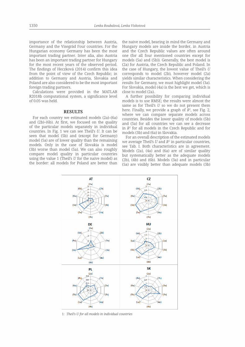
and (2b)–(6b). At first, we focused on the quality of the particular models separately in individual countries. In Fig. 1 we can see Theil’s U. It can be seen that model (5b) and (except for Germany) model (5a) are of lower quality than the remaining models. Only in the case of Slovakia is model (3b) worse than model (5a). We can also roughly compare model quality in particular countries using the value 1 (Theil’s U for the naive model) as the border: all models for Poland are better than

the naive model, bearing in mind the Germany and Hungary models are inside the border, in Austria and the Czech Republic values are often around one (for all four mentioned countries except for models (5a) and (5b)). Generally, the best model is (2a) for Austria, the Czech Republic and Poland. In the case of Hungary, the lowest value of Theil’s U corresponds to model (2b), however model (2a) yields similar characteristics. When considering the results for Germany, we must highlight model (3a). For Slovakia, model (4a) is the best we get, which is close to model (2a).

A further possibility for comparing individual models is to use RMSE; the results were almost the same as for Theil’s U so we do not present them here. Finally, we provide a graph of R2, see Fig. 2, where we can compare separate models across countries. Besides the lower quality of models (5b) and (5a) for all countries we can see a decrease in R2 for all models in the Czech Republic and for models (3b) and (6a) in Slovakia.

For an overall description of the estimated models we average Theil’s U and R2 in particular countries, see Tab. I. Both characteristics are in agreement. Models (2a), (4a) and (6a) are of similar quality but systematically better as the adequate models (2b), (4b) and (6b). Models (3a) and in particular (5a) are visibly better than adequate models (3b)

Republic and Poland. In the case of Hungary, the lowest value of Theil’s U corresponds to 185

model (2b), however model (2a) yields similar characteristics. When considering the results 186

for Germany, we must highlight model (3a). For Slovakia, model (4a) is the best we get, 187

which is close to model (2a). 188

189

Figure 1 Theil’s U for all models in individual countries. 190

A further possibility for comparing individual models is to use RMSE; the results were almost 191

the same as for Theil’s U so we do not present them here. Finally, we provide a graph of R2, 192

see Fig. 2, where we can compare separate models across countries. Besides the lower quality 193

of models (5b) and (5a) for all countries we can see a decrease in R2 for all models in the 194

Czech Republic and for models (3b) and (6a) in Slovakia. 195

1: Theil’s U for all models in individual countries


and (5b). We can denote model (2a) as the best model generally; country-dependent details will be discussed later, see Tab. III.

Beside the quality of the models, it is necessary to investigate the statistical signifi cance of parameters related to changes in time, i.e. parameters a1, b1 and c1, see Tab. II. Except for model (4a) the parameters appropriate for the individual models

are statistically signifi cant for at least one country. Generally, the best model (2a) according to average Theil’s U has all time-related parameters insignifi cant for the Czech Republic, Germany, Hungary and Slovakia. For Germany we obtain (3a) as the better model. For the remaining countries this insignifi cance points out to the model (2b), which can be slightly worse according to Theil’s U, but having at least one signifi cant time-related parameter.

DISCUSSIONThe time augmented production function can be

found in papers by Makin and Strong (2013) dealing with the problem of the elasticity of substitution between capital and labour and factor productivity in Australia and in the paper by Roubalová and Viskotová (2018) where productivity development

196

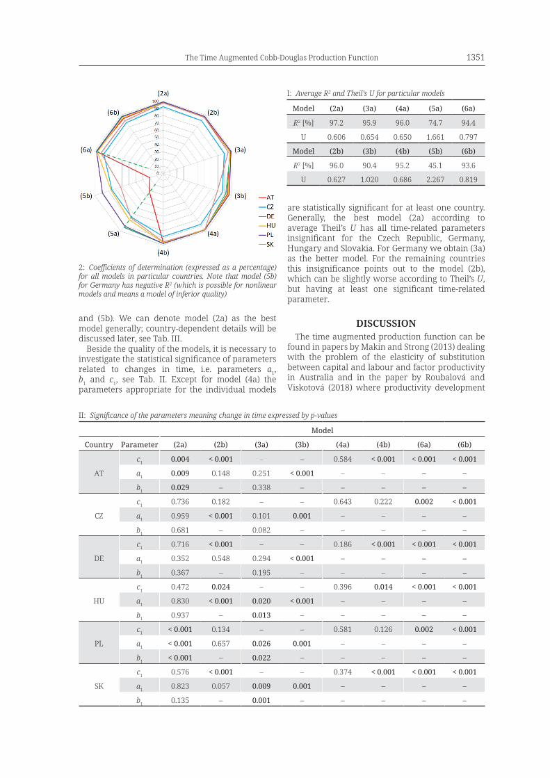
Figure 2 Coefficients of determination (expressed as a percentage) for all models in particular 197

countries. Note that model (5b) for Germany has negative R2 (which is possible for nonlinear models 198

and means a model of inferior quality).199

For an overall description of the estimated models we average Theil’s U and R2 in particular 200

countries, see Tab. I. Both characteristics are in agreement. Models (2a), (4a) and (6a) are of201

similar quality but systematically better as the adequate models (2b), (4b) and (6b). Models 202

(3a) and in particular (5a) are visibly better than adequate models (3b) and (5b). We can 203

denote model (2a) as the best model generally; country-dependent details will be discussed 204

later, see Tab. III.205

Model (2a) (3a) (4a) (5a) (6a)R2 [%] 97.2 95.9 96.0 74.7 94.4U 0.606 0.654 0.650 1.661 0.797Model (2b) (3b) (4b) (5b) (6b)R2 [%] 96.0 90.4 95.2 45.1 93.6U 0.627 1.020 0.686 2.267 0.819

Table I Average R2 and Theil’s U for particular models.206

Beside the quality of the models, it is necessary to investigate the statistical significance of 207

parameters related to changes in time, i.e. parameters 𝑎𝑎𝑎𝑎1, 𝑏𝑏𝑏𝑏1 and 𝑐𝑐𝑐𝑐1, see Tab. II. Except for208

model (4a) the parameters appropriate for the individual models are statistically significant for 209

at least one country. Generally, the best model (2a) according to average Theil’s U has all 210

time-related parameters insignificant for the Czech Republic, Germany, Hungary and 211

Slovakia. For Germany we obtain (3a) as the better model. For the remaining countries this 212

insignificance points out to the model (2b), which can be slightly worse according to Theil’s 213

U, but having at least one significant time-related parameter.214

2: Coefficients of determination (expressed as a percentage) for all models in particular countries. Note that model (5b) for Germany has negative R2 (which is possible for nonlinear models and means a model of inferior quality)

II: Signifi cance of the parameters meaning change in time expressed by p-values

Model

Country Parameter (2a) (2b) (3a) (3b) (4a) (4b) (6a) (6b)

AT

c1 0.004 < 0.001 – – 0.584 < 0.001 < 0.001 < 0.001

a1 0.009 0.148 0.251 < 0.001 – – – –

b1 0.029 – 0.338 – – – – –

CZ

c1 0.736 0.182 – – 0.643 0.222 0.002 < 0.001

a1 0.959 < 0.001 0.101 0.001 – – – –

b1 0.681 – 0.082 – – – – –

DE

c1 0.716 < 0.001 – – 0.186 < 0.001 < 0.001 < 0.001

a1 0.352 0.548 0.294 < 0.001 – – – –

b1 0.367 – 0.195 – – – – –

HU

c1 0.472 0.024 – – 0.396 0.014 < 0.001 < 0.001

a1 0.830 < 0.001 0.020 < 0.001 – – – –

b1 0.937 – 0.013 – – – – –

PL

c1 < 0.001 0.134 – – 0.581 0.126 0.002 < 0.001

a1 < 0.001 0.657 0.026 0.001 – – – –

b1 < 0.001 – 0.022 – – – – –

SK

c1 0.576 < 0.001 – – 0.374 < 0.001 < 0.001 < 0.001

a1 0.823 0.057 0.009 0.001 – – – –

b1 0.135 – 0.001 – – – – –

I: Average R2 and Theil’s U for particular models

Model (2a) (3a) (4a) (5a) (6a)

R2 [%] 97.2 95.9 96.0 74.7 94.4

U 0.606 0.654 0.650 1.661 0.797

Model (2b) (3b) (4b) (5b) (6b)

R2 [%] 96.0 90.4 95.2 45.1 93.6

U 0.627 1.020 0.686 2.267 0.819


in selected Central European countries was investigated. In both papers the non-CES production function defined by Sato (1964) and Sato (1970) was used. The Sato production function is linearly homogeneous and exhibits constant returns to scale. There are also advantages related to the Sato specification: there is no assumption of the constant elasticity of substitution, it contains a relatively low number of parameters, and the inverse transformation can be used to linearize it.

Time augmentation of the Sato production function enables derivation of characteristics changing in time. In Roubalová and Viskotová (2018) the estimations for the time augmented production functions proved that the labour and capital input combination had changed during the observed period 1995–2005 and labour-saving or capital-saving technological progress was identified for the countries investigated.

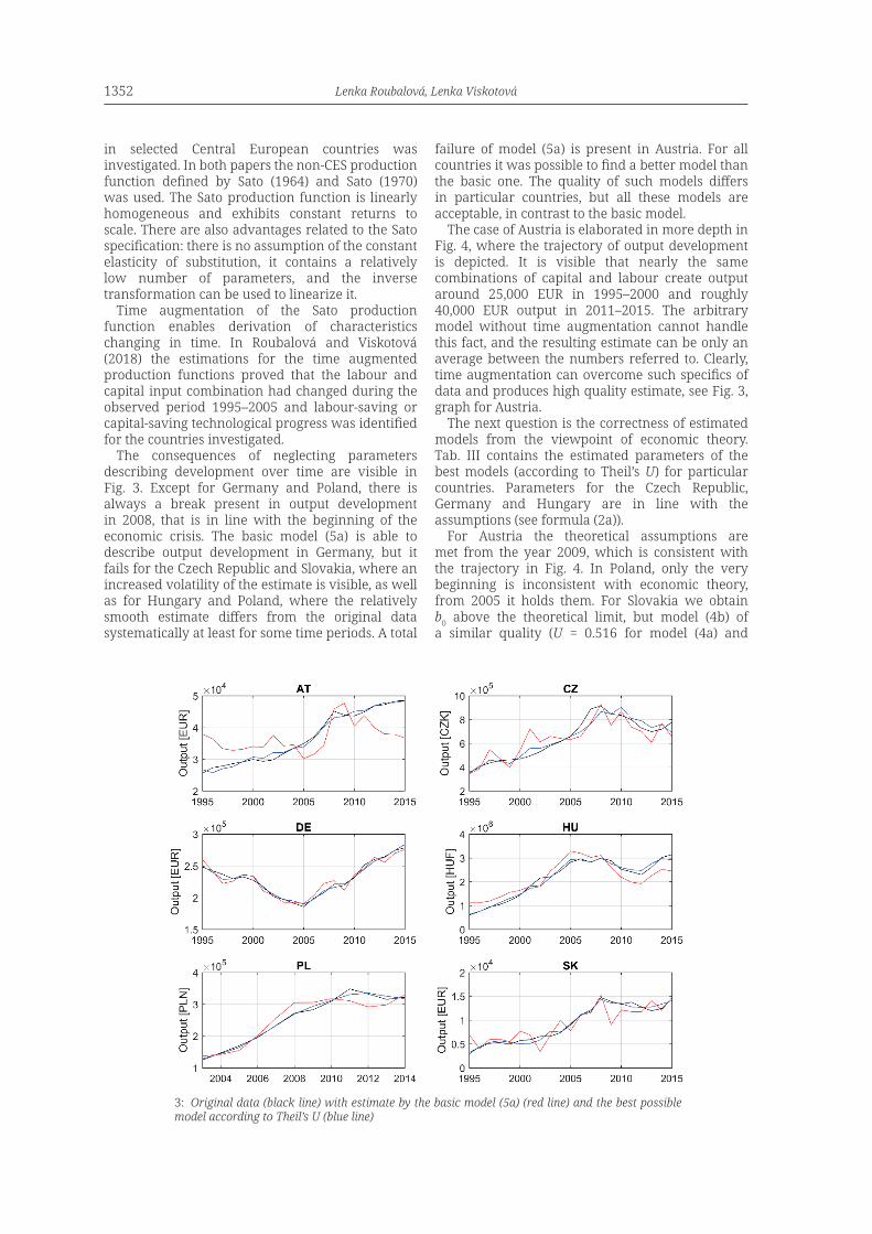
The consequences of neglecting parameters describing development over time are visible in Fig. 3. Except for Germany and Poland, there is always a break present in output development in 2008, that is in line with the beginning of the economic crisis. The basic model (5a) is able to describe output development in Germany, but it fails for the Czech Republic and Slovakia, where an increased volatility of the estimate is visible, as well as for Hungary and Poland, where the relatively smooth estimate differs from the original data systematically at least for some time periods. A total

failure of model (5a) is present in Austria. For all countries it was possible to find a better model than the basic one. The quality of such models differs in particular countries, but all these models are acceptable, in contrast to the basic model.

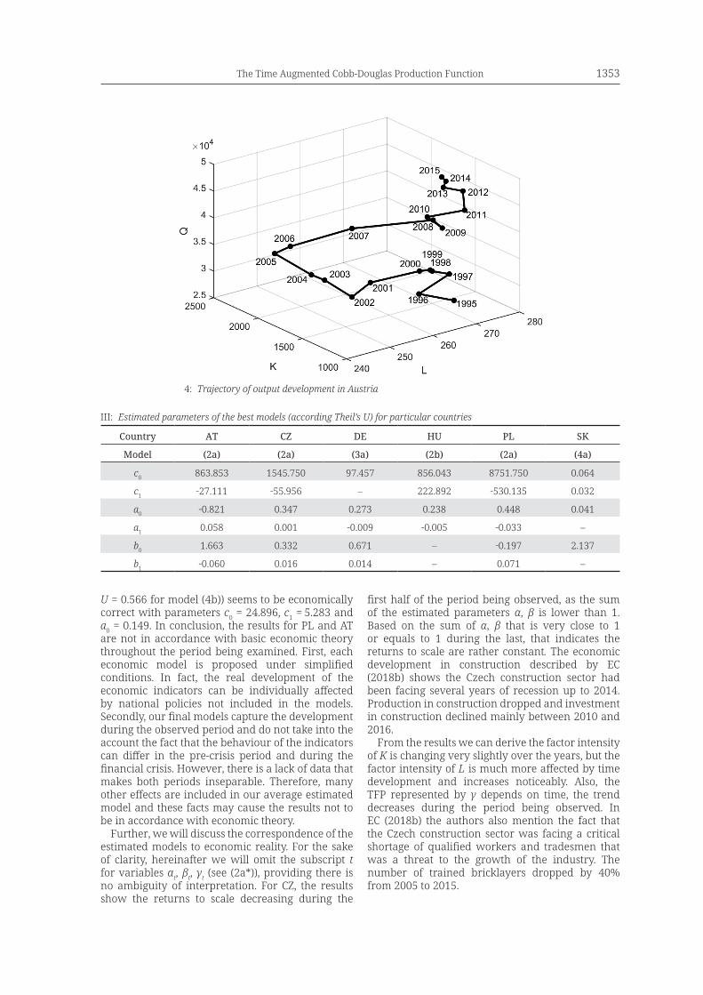
The case of Austria is elaborated in more depth in Fig. 4, where the trajectory of output development is depicted. It is visible that nearly the same combinations of capital and labour create output around 25,000 EUR in 1995–2000 and roughly 40,000 EUR output in 2011–2015. The arbitrary model without time augmentation cannot handle this fact, and the resulting estimate can be only an average between the numbers referred to. Clearly, time augmentation can overcome such specifics of data and produces high quality estimate, see Fig. 3, graph for Austria.

The next question is the correctness of estimated models from the viewpoint of economic theory. Tab. III contains the estimated parameters of the best models (according to Theil’s U) for particular countries. Parameters for the Czech Republic, Germany and Hungary are in line with the assumptions (see formula (2a)).

For Austria the theoretical assumptions are met from the year 2009, which is consistent with the trajectory in Fig. 4. In Poland, only the very beginning is inconsistent with economic theory, from 2005 it holds them. For Slovakia we obtain b0 above the theoretical limit, but model (4b) of a similar quality (U = 0.516 for model (4a) and

The consequences of neglecting parameters describing development over time are visible in 232

Fig. 3. Except for Germany and Poland, there is always a break present in output development 233

in 2008, that is in line with the beginning of the economic crisis. The basic model (5a) is able 234

to describe output development in Germany, but it fails for the Czech Republic and Slovakia, 235

where an increased volatility of the estimate is visible, as well as for Hungary and Poland, 236

where the relatively smooth estimate differs from the original data systematically at least for 237

some time periods. A total failure of model (5a) is present in Austria. For all countries it was 238

possible to find a better model than the basic one. The quality of such models differs in 239

particular countries, but all these models are acceptable, in contrast to the basic model. 240

241

Figure 3 Original data (black line) with estimate by the basic model (5a) (red line) and the best 242

possible model according to Theil’s U (blue line). 243

The case of Austria is elaborated in more depth in Fig. 4, where the trajectory of output 244

development is depicted. It is visible that nearly the same combinations of capital and labour 245

create output around 25,000 EUR in 1995–2000 and roughly 40,000 EUR output in 2011–246

2015. The arbitrary model without time augmentation cannot handle this fact, and the 247

resulting estimate can be only an average between the numbers referred to. Clearly, time 248

3: Original data (black line) with estimate by the basic model (5a) (red line) and the best possible model according to Theil’s U (blue line)


U = 0.566 for model (4b)) seems to be economically correct with parameters c0 = 24.896, c1 = 5.283 and a0 = 0.149. In conclusion, the results for PL and AT are not in accordance with basic economic theory throughout the period being examined. First, each economic model is proposed under simplified conditions. In fact, the real development of the economic indicators can be individually affected by national policies not included in the models. Secondly, our final models capture the development during the observed period and do not take into the account the fact that the behaviour of the indicators can differ in the pre-crisis period and during the financial crisis. However, there is a lack of data that makes both periods inseparable. Therefore, many other effects are included in our average estimated model and these facts may cause the results not to be in accordance with economic theory.

Further, we will discuss the correspondence of the estimated models to economic reality. For the sake of clarity, hereinafter we will omit the subscript t for variables αt, βt, γt (see (2a*)), providing there is no ambiguity of interpretation. For CZ, the results show the returns to scale decreasing during the

first half of the period being observed, as the sum of the estimated parameters α, β is lower than 1. Based on the sum of α, β that is very close to 1 or equals to 1 during the last, that indicates the returns to scale are rather constant. The economic development in construction described by EC (2018b) shows the Czech construction sector had been facing several years of recession up to 2014. Production in construction dropped and investment in construction declined mainly between 2010 and 2016.

From the results we can derive the factor intensity of K is changing very slightly over the years, but the factor intensity of L is much more affected by time development and increases noticeably. Also, the TFP represented by γ depends on time, the trend decreases during the period being observed. In EC (2018b) the authors also mention the fact that the Czech construction sector was facing a critical shortage of qualified workers and tradesmen that was a threat to the growth of the industry. The number of trained bricklayers dropped by 40% from 2005 to 2015.

augmentation can overcome such specifics of data and produces high quality estimate, see 249

Fig. 3, graph for Austria. 250

251

Figure 4 Trajectory of output development in Austria. 252

The next question is the correctness of estimated models from the viewpoint of economic 253

theory. Tab. III contains the estimated parameters of the best models (according to Theil’s U) 254

for particular countries. Parameters for the Czech Republic, Germany and Hungary are in line 255

with the assumptions (see formula (2a)). 256

Country AT CZ DE HU PL SK Model (2a) (2a) (3a) (2b) (2a) (4a)

c0 863.853 1545.750 97.457 856.043 8751.750 0.064

c1 -27.111 -55.956 ─ 222.892 -530.135 0.032

a0 -0.821 0.347 0.273 0.238 0.448 0.041

a1 0.058 0.001 -0.009 -0.005 -0.033 ─

b0 1.663 0.332 0.671 ─ -0.197 2.137

b1 -0.060 0.016 0.014 ─ 0.071 ─ 257

Table III Estimated parameters of the best models (according Theil’s U) for particular countries. 258

For Austria the theoretical assumptions are met from the year 2009, which is consistent with 259

the trajectory in Fig. 4. In Poland, only the very beginning is inconsistent with economic 260

4: Trajectory of output development in Austria

III: Estimated parameters of the best models (according Theil’s U) for particular countries

Country AT CZ DE HU PL SK

Model (2a) (2a) (3a) (2b) (2a) (4a)

c0 863.853 1545.750 97.457 856.043 8751.750 0.064

c1 -27.111 -55.956 – 222.892 -530.135 0.032

a0 -0.821 0.347 0.273 0.238 0.448 0.041

a1 0.058 0.001 -0.009 -0.005 -0.033 –

b0 1.663 0.332 0.671 – -0.197 2.137

b1 -0.060 0.016 0.014 – 0.071 –


The same kind of the development of γ was found for AT and PL. Construction is the only industry with negative growth in added value over the period being investigated. This is primarily a result of huge downturns in the second half of the 1990s. Since then, the economic performance of this sector has been relatively solid, showing the features of capital-driven growth. As our results show, for AT, DE, HU and SK there is a decisive impact of labour.

In Roubalová and Viskotová (2018) we proved that capital-saving technological progress at country level is present in SK and DE, which means that technological progress is driven by knowledge and workforce improvement. These results are also in accordance with conclusions reached in Biea (2016). A similar statement can be found in Kotulic et al. (2015), where the analysis for 1995–2012 confirmed a strong dependence between employment and the economic performance and productivity of the Slovak economy. According to the European Commission (EC) (2018c) the number of people employed in the construction sector in DE increased substantially (30.6%) between 2010 and 2016. In the case of DE we can also notice that the model where γ is not a function of time is preferred. This means that the level of technology is relatively constant. There are sources supporting this result, e.g. Naudé and Nagler (2017), who argue that there is a decline in the effectiveness of technological innovation during 1991–2015. They revealed three reasons why technological innovation is not a driving force for inclusive economic growth in Germany: historical legacies, weaknesses in the education system, and entrepreneurial stagnation.

For HU, the results are similar and also supported by the information from the EC (2018d). This reports a 11.5% decrease in total production from 2010 to 2016 and a 7.5% decrease in workers employed in the construction sector in 2015 with respect to the situation in 2010. However, overall labour productivity experienced an increment of 20.6% in this period, while the largest increase in productivity in construction was experienced in 2010.

For SK (model (4b)) and HU (model (2b)) we have constant returns to scale. For DE, the returns to scale are relatively constant, because the sum of α, β is very close to 1.

For PL, we can see changing impact of α and β. The sign for factor intensity of labour β is even negative, which is not in accordance with economic theory. We can build an explanation partly on the facts mentioned by the EC (2018e). According to this document the structure of the construction sector in PL differs from that in other countries. The Polish construction sector is composed mostly of small companies and only several larger players. In labour productivity we find a sharp decline in 2010–2013, following which it was increasing. As the EC (2018e) shows, as a result of this development, production was fluctuating in the second half of the analysed period that was accompanied by a fall in employment that reached a level below that of 2010. As the EC (2018e) reports, business confidence had been improving in this sector steadily for last eight years and despite the uncertainty about the development in construction, investment per worker grew steadily at least from 2010 to 2015.

We can find here also a kind of explanation for α. As the EC (2018e) shows, during the last five years of the analysed period economic growth was sluggish which was linked to a low level of foreign investment. However, loans to non-financial corporations increased substantially from 2010 as well as the expectations related to growth in future being positive.

The results for AT are also in contrary to basic economic theory, because we revealed a negative α in the model and quite a high value for β before 2009. As the EC (2018a) states, the economic crisis affected business confidence in the economy in AT in a significant manner. Namely, construction confidence had stood at 14.7 in 2010 followed by a decline to -16.2 in 2014. In parallel, based on increasing input material prices, construction costs had been increasing. On the other hand, this report also points out that labour productivity in the construction sector experienced a 5.5% increase between 2010 and 2013, from EUR 65,200 to EUR 68,800. Architectural activity also experienced a 6.3% increment in productivity during this period as well as the manufacturing subsector, which experienced the highest productivity growth of all the subsectors EC (2018a).

CONCLUSIONOur results prove the time augmented version of the CDPF yields better results than the basic one. In most cases, all parameters are changing over time and this change is statistically significant. Our analysis shows that the best versions of the augmented CDPF describing the production relationship in construction industry in these countries are versions given by equations (2a)–(4a), and model with constant returns to scale (2b). In the case of models with constant returns to scale we almost always receive higher Theil’s U than for adequate models neglecting this property. Our analysis even proved, if there are countries with some specific characters in the development, in our case AT and PL, the model is not able to describe it successfully across the full time range.


The time augmented Cobb-Douglas function is able to capture technological progress over time and distinguish how fast it is on the basis of time dependent parameters. It is also able to distinguish the contribution of labour and capital inputs. Finally, the basic Cobb-Douglas production function is very popular mainly because of the fact it is quite easy to estimate it and interpret its parameters. However, the simplicity of the estimation is compensated by the simplistic assumption which might be far from the real development observed in the real economy, but which is necessary to model with the time augmented CDPF. Further research could be focused on other individual sectors to describe the production relationship by the other time augmented production functions to see the differences and common characteristics in development captured by several various kinds of the production function specification.

REFERENCESALKHAREIF, R. M., BARNETT, W. A. and ALSADOUN, N. A. 2017. Estimating the Output Gap for Saudi

Arabia. International Journal of Economics and Finance, 9(3): 81–90. BIEA, N. 2016. Economic growth in Slovakia: Past successes and future challenges. Economic brief 008.

Luxembourg: Publications Office of the European Union. BESANKO, D. and BRAEUTIGAM, R. 2007. Microeconomics. 3rd Edition. Canada: John Willey & Sons.COBB, C. W. and DOUGLAS, P. H. 1928. A Theory of Production. American Economic Review, 18: 139–

165.COTIS, J. P., ELMESKOV, J. and MOUROUGANE, A. 2005. Estimates of potential output: benefits and

pitfalls from a policy perspective. In: Rechling, L. (Ed.). Euro Area Business Cycles: Stylized Facts and Measurement Issues. London: CEPR.

ČERNÝ, J. 2011. Comparison of Cobb-Douglas Production Functions of the Chosen Countries by Using Econometric Model. In: Proceedings of the 29th International Conference on Mathematical Methods in Economics 2011 – part I. University of Economics, 6–9 September. Prague: Professional Publishing, pp. 107–112.

D’AURIA, F. 2010. The production function methodology for calculating potential growth rates and output gaps. Brussels: European Commission, Directorate-General for Economic and Financial Affairs.

EUROPEAN COMMISSION. 2016. EU’s top trading partners in 2015: the UnitedStates for exports, China for imports. Pressrelase. Eurostat Press Office. Available at: http://ec.europa.eu/eurostat/documents/2995521/7224419/6-31032016-BPEN.pdf/b82ea736-1c73-487f-8fb5-4954774bb63a [Accessed: 2019, August 11].

EUROPEAN COMISSION. 2018a. European Construction Sector Observatory, Country Profile Austria. [Online]. Available at: https://ec.europa.eu/docsroom/documents/30286/attachments/1/translations/en/renditions/pdf [Accessed: 2019, July 22].

EUROPEAN COMISSION. 2018b. European Construction Sector Observatory, Country Profile Czech Republic. [Online]. Available at: https://ec.europa.eu/docsroom/documents/30287/attachments/1/translations/en/renditions/pdf. [Accessed: 2019, July 22].

EUROPEAN COMISSION. 2018c. European Construction Sector Observatory, Country Profile Germany. [Online]. Available at: https://ec.europa.eu/docsroom/documents/23744/attachments/1/translations/en/renditions/pdf. [Accessed: 2019, July 22].

EUROPEAN COMISSION. 2018d. European Construction Sector Observatory, Country Profile Hungary. [Online]. Available at: https://ec.europa.eu/docsroom/documents/30348/attachments/1/translations/en/renditions/pdf. [Accessed: 2019, July 22].

EUROPEAN COMISSION. 2018e. European Construction Sector Observatory, Country Profile Poland. [Online]. Available at: https://ec.europa.eu/docsroom/documents/30668/attachments/1/translations/en/renditions/pdf. [Accessed: 2019, July 22].

GREENE, W. H. 2012. Econometric analysis. 7th Edition. Boston: Pearson. HÁJKOVÁ, D. and HURNÍK J. 2007. Cobb-Douglas Production Function: The Case of a Converging

Economy. Finance a úvěr, 57(9–10): 465–476. HECZKOVÁ, M. 2014. Fakta o obchodě se zahraničím. Statistika & My, 9: 19–20.KMENTA, J. 1967. On Estimation of the CES Production Function. International Economic Review, 8(2):

180–189.KMENTA, J. 1990. Elements of Econometrics. 2nd Edition. New York: Macmillan.KOTULIC, R., KRAVČÁKOVÁ VOZÁROVÁ, I., NAGY, J., HUTTMANOVÁ, E. and VAVREČKA, R. 2015.

Performance of The Slovak Economy in Relation to Labor Productivity and Employment. Economics and Finance, 23: 970–975.


LEVENBERG, K. 1944. A Method for the Solution of Certain Non-Linear Problems in Least Squares. Quarterly of Applied Mathematics, 2: 164–168.

MAKIN, J. A. and STRONG, S. 2013. New Measures of Factor Productivity in Australia: a Sato approach. Applied Economics Australia, 45(17): 2413–2422.

MARQUARDT, D. 1963. An Algorithm for Least-Squares Estimation of Nonlinear Parameter. Journal of the Society for Industrial and Applied Mathematics, 11(2): 431–441.

MISHRA, S. K. 2007. A Brief History of Production Functions. The IUP Journal of Managerial Economics, 8(4): 6–34.

NAUDÉ, W. and NAGLER, P. 2017. Technological Innovation and Inclusive Growth in Germany. IZA Discussion Paper Series, 11194. IZA Institute of Labor Economics.

RÕÕM, M. 2001. Potential Output Estimates for Central and East European Countries Using Production Function Method. Working Papers of Eesti Pank, 2: 1–23. Eesti Pank.

ROUBALOVÁ, L., HAMPEL, D. and VISKOTOVÁ, L. 2018. Technological Progress at the Sectoral Level: the Sato Production Function Approach. In: Proceedings of the 36th International Conference on Mathematical Methods in Economics. University of Economics, 12–14 September. Prague: Professional Publishing, pp. 470–475.

ROUBALOVÁ, L. and VISKOTOVÁ, L. 2018. Productivity Development in Selected Central European Countries Measured by the Sato Production Function. Review of economic perspectives, 18(4): 353–370.

SATO, R. 1964. Diminishing returns and linear homogeneity: comment. The American Economic Review, 54(5): 744–745.

SATO, R. 1970. The Estimation of Biased Technical Progress and the Production Function. International Economic Review, 11(2): 179–208.

THEIL, H. 1966. Applied Economic Forecasting. Amsterdam: North-Holland.VISKOTOVÁ, L., ROUBALOVÁ, L. and HAMPEL, D. 2019. Starting Parameters For The Estimation Of

The Production Functions. In: Proceedings of the 16th International Conference of Numerical Analysis and Applied Mathematics (ICNAAM 2018). Rhodes, Greece 13–18 September. Melville: American Institute of Physics (AIP).

ZIMKOVÁ, E. and BAROCHOVSKÝ, J. 2007. Odhad potenciálneho produktu a produkčnej medzery v slovenských podmienkach. Politická ekonomie, 4: 473–489.

Contact informationLenka Roubalová: [email protected] Viskotová: [email protected]

(PDF) The Time Augmented Cobb-Douglas Production Function

Documents